Forthcoming Review of Financial Studies

Does the Source of Capital Affect Capital Structure?

Michael FaulkenderOlin School of Business, Washington University in St. Louis

and

Mitchell A. PetersenKellogg School of Management, Northwestern University

and NBER

Petersen thanks the Financial Institutions and Markets Research Center at Northwestern University’sKellogg School for support. We also appreciate the suggestions and advice of Allen Berger, CharlesCalomiris, Mark Carey, Kent Daniel, Gary Gorton, John Graham, Elizabeth Henderson, AhmetKocagil, Vojislav Maksimovic, Geoff Mattson, Bob McDonald, Hamid Mehran, Todd Milbourn,Rob O’Keef, Todd Pulvino, Doug Runte, Jeremy Stein, Chris Struve, Sheridan Titman, Greg Udell,and Jeff Wurgler, as well as seminar participants at the Conference on Financial Economics andAccounting, the Financial Intermediation Research Society Conference on Banking, Insurance andIntermediation, the Federal Reserve Bank of Chicago’s Bank Structure Conference, the NationalBureau of Economic Research, the American Finance Association, Moody’s Investors Services,Northwestern University, the World Bank, Yale University, and the Universities of Colorado,Laussane, Minnesota, Missouri, Oxford, Rochester, and Virginia. The views expressed in this paperare those of the authors. The research assistance of Eric Hovey, Jan Zasowski, Tasuku Miuri,Sungjoon Park, and Daniel Sheyner is greatly appreciated.

Abstract

Prior work on leverage implicitly assumes capital availability depends solely on firm

characteristics. However, market frictions that make capital structure relevant may be associated

with a firm's source of capital. Examining this intuition, we find firms which have access to the

public bond markets, as measured by having a debt rating, have significantly more leverage.

Although firms with a rating are fundamentally different, these differences do not explain our

findings. Even after controlling for firm characteristics which determine observed capital structure,

and instrumenting for the possible endogeneity of having a rating, firms with access have 35 percent

more debt.

1

I) Introduction

Under the tradeoff theory of capital structure, firms determine their preferred leverage ratio

by calculating the tax advantages, costs of financial distress, mispricing, and incentive effects of debt

versus equity. The empirical literature has searched for evidence that firms choose their capital

structure as this theory predicts by estimating firm leverage as a function of firm characteristics.

Firms for whom the tax shields of debt are greater, the costs of financial distress lower, and the

mispricing of debt relative to equity more favorable are expected to be more highly levered. When

these firms discover that the net benefit of debt is positive, they will move toward their preferred

capital structure by issuing additional debt and/or reducing their equity. The implicit assumption has

been that a firm’s leverage is completely a function of the firm’s demand for debt. In other words,

the supply of capital is infinitely elastic at the correct price and the cost of capital depends only upon

the risk of the firm’s projects.

Although the empirical literature has been successful, in the sense that many of the proposed

proxies are correlated with firms’ actual capital structure choices, some authors have argued that

certain firms appear to be significantly under-levered. For example, based on estimated tax benefits

of debt, Graham (2000) argues that firms appear to be missing the opportunity to create significant

value by increasing their leverage and thus reducing their tax payments, assuming that the other

costs of debt have been measured correctly.1 This interpretation assumes that firms have the

opportunity to increase their leverage and are choosing to leave money on the table. An alternative

explanation is that firms may not be able to issue additional debt. The same type of market frictions

that make capital structure choices relevant (information asymmetry and investment distortions) also

imply that firms sometimes are rationed by their lenders (Stiglitz and Weiss, 1981). Thus, when

2

estimating a firm’s leverage, it is important to include not only the determinants of its preferred

leverage (the demand side) but also the variables that measure the constraints on a firm’s ability to

increase its leverage (the supply side).

The literature often has described banks or private lenders as being particularly good at

investigating informationally-opaque firms and deciding which are viable borrowers. This suggests

that the source of capital may be intimately related to a firm’s ability to access debt markets. Firms

that are opaque (and thus difficult to investigate ex-ante), or that have more discretion in their

investment opportunities (and thus are difficult for lenders to constrain contractually), are more

likely to borrow from active lenders; they are also the type of firms that theory predicts may be

credit constrained. In this paper, we investigate the link between where firms obtain their capital (the

private versus public debt markets) and their capital structure (leverage ratio). In the next section,

we briefly describe the tradeoff between financial intermediaries (the private debt markets), which

have an advantage at collecting information and restructuring but are a potentially more expensive

source of capital, and the public debt markets. The higher cost of private debt capital may arise from

the expenditure on monitoring or because of the tax disadvantage of the lender’s organizational form

(Graham, 1999). Additionally, not all firms may be able to choose the source of their debt capital.

If firms that do not have access to the public debt markets are constrained by lenders as to the

amount of debt capital they may raise, then we should see this manifest itself in the form of lower

debt ratios. This is what we find in Section II. Firms that have access to the public debt markets

(defined as having a debt rating) have leverage ratios that are more than 50 percent higher than firms

that do not have access (28.4 versus 17.9 percent).

Debt ratios should depend upon firm characteristics as well. Thus, a difference in leverage

3

does not necessarily imply that firms are constrained by the debt markets. The difference could be

the product of firms with different characteristics optimally making different decisions about

leverage. However, this does not appear to be the case. In Section III, we show that even after

controlling for the firm characteristics – which theory and previous empirical work argue determine

a firm’s choice of leverage – firms with access to the public debt market have higher leverage that

is both economically and statistically significant.

Finally, in Section IV we consider the possibility that access to the public debt markets

(having a debt rating) is endogenous. Even after controlling for the endogeneity of a debt rating, we

find that firms with access to the public debt markets have significantly higher leverage ratios.

II) Empirical Strategy and the Basic Facts

A) Relationship versus Arm’s Length Lending

In a frictionless capital market, firms are always able to secure funding for positive net

present value (NPV) projects. But in the presence of information asymmetry in which the firm’s

quality and the quality of its investment projects cannot easily be evaluated by outside lenders, firms

may not be able to raise sufficient capital to fund all of their good projects (Stiglitz and Weiss,

1981).2 Such market frictions create the possibility for differentiated financial markets or institutions

to arise (Leland and Pyle, 1977; Diamond, 1984; Ramakrishnan and Thakor, 1984; Fama, 1985;

Haubrich, 1989; and Diamond 1991). These financial intermediaries are lenders who specialize in

collecting information about borrowers which they then use in the credit approval decision (Carey,

Post, and Sharpe, 1998). By interacting with borrowers over time and across different products, the

financial intermediary may be able to partially alleviate the information asymmetry that causes the

market’s failure. These financial relationships have been empirically documented to be important

4

in relaxing capital constraints (Hoshi, Kashyap and Scharfstein, 1990a, 1990b; Petersen and Rajan,

1994, 1995; and Berger and Udell, 1995).

Financial intermediaries (e.g. banks) also may have an advantage over arm’s length lenders

(e.g. bond markets) after the capital is provided. If ex-post monitoring raises the probability of

success (through either enforcing efficient project choice or the expenditure of the owner’s effort),

then they may be a preferred source of capital (Diamond, 1991; Mester, Nakamura, and Renault,

2004). In addition, financial intermediaries may be more efficient at restructuring firms that are in

financial distress (Rajan, 1992; Bolton and Scharfstein, 1996, Bolton and Freixas, 2000).

This intuition is the basis for the empirical literature that examines firms’ choices of lenders.

Firms that are riskier (more likely to need to be restructured), smaller, and about whom less is

known are those most likely to borrow from financial intermediaries (Cantillo and Wright, 2000;

Faulkender, 2004; Petersen and Rajan, 1994). Larger firms, about which much is known, will be

more likely to borrow from arm’s length capital markets.

However, the monitoring that is done by financial intermediaries and the resources devoted

to restructuring firms are costly. This cost must be passed back to the borrower. It means that the

cost of capital for firms in such an imperfect market depends not only on the risk of their projects

but also on the resources needed to verify the viability of their projects. Although the institutional

response (the development of financial intermediaries and lending relationships) can partially

mitigate the market distortions, it is unlikely that these distortions are eliminated completely. If

monitoring is costly and imperfect, then for two firms with identical projects, the one that needs to

be monitored (for example, an entrepreneur without a track record) will find that the cost of debt

capital is higher. The cost of monitoring will be passed on to the borrower in the form of higher

5

QDemand ' α0 Price % α1 XDemand factors % εDQSupply ' β0 Price % β1 XSupply factors % εS

(1)

interest rates, causing the firm to reduce its use of debt capital. In addition, if the monitoring and

additional information collection performed by the financial intermediary cannot completely

eliminate the information asymmetry, then credit still may be rationed. So, if we compare firms that

are able to borrow from the bond market with those that cannot, we will find that firms with access

to the bond market have more leverage. This result can occur directly through a quantity channel

(lenders who are willing to lend more) or indirectly through a price channel (firms with access to

a cheaper source of capital borrow more). Either way, opening a new supply of capital to a firm will

increase the firm’s leverage.

B) Empirical Strategy

To examine the role of credit constraints and help to explore the difference between the

public debt markets (e.g. bonds) and the private debt market (e.g. banks), we consider the leverage

of firms to be a function of the firm’s capital market access. If firms without access to public debt

markets are constrained in the amount of debt they may issue, then they should be less levered, even

after controlling for other determinants of capital structure. The observed level of debt is a function

of the supply of debt and the firm’s demand for debt, both of which depend on the price of debt

capital and supply and demand factors.

If there are no supply frictions, then firms can borrow as much debt as they want (at the correct

price), and the observed level of debt will equal the demanded level. This is the traditional

assumption in the empirical capital structure literature. Only demand factors explain variation in the

firm’s debt level, where demand factors are any firm characteristic that raises the net benefit of debt.

6

QObserved ' γD XDemand factors % γS XSupply factors % µ' γD XDemand factors % γS Bond market access % µ (2)

Some examples of these are higher marginal tax rates and lower costs of financial distress.

However, if firms without access to public debt markets are constrained in the amount of

debt that they may issue (private lenders do not fully replace the lack of public debt), then they will

have lower leverage ratios, even after controlling for the firm’s demand for debt. Equating the

demand and supply, we can express the above equations as two reduced-form equations – one for

quantity and one for price – so that each is only a function of the demand and supply factors.

This is the regression that we run throughout the paper. We examine whether firms that have access

to public debt markets have access to a greater supply of debt, and thus are more highly levered. We

use whether the firm has a bond rating or a commercial paper rating as a measure of access to the

public bond markets. Previous research on the source of debt capital has focused on small, hand

collected data samples to accurately document the source of each of the firm’s debt issuances

(Houston and James, 1996; Cantillo and Wright, 2000). In these samples, the correspondence

between having a debt rating and having public debt outstanding is quite high. Very few firms

without a debt rating have public debt and very few firms have a debt rating but no public debt.3

Although having a bond rating is an indication of having access to the bond market, the two

are not exactly the same. Firms may not have a debt rating, either because they don’t have access

to the bond market or because they do not want a debt rating or public debt (see Figure 1). Thus in

equation (2) a positive coefficient on having a rating could be either the supply effect we are testing

for or unobserved demand factors that are correlated with having a rating. To argue that the bond

rating variable in fact is a supply variable, we use two separate approaches. First, we control for firm

7

characteristics that measure the amount of debt a firm would like to have. If we could completely

control for variation in the demand for debt with our other independent variables, then the rating

variable would only measure variation in supply. After controlling for observed and unobserved

variation in firm characteristics (demand factors), we find that leverage is significantly higher for

firms with a rating. These results are reported in Section III.

Our second approach is to examine the variation in supply directly. We do this by estimating

an instrumental variables version of the model. By first predicting which firms are able to access the

public bond markets, we can distinguish between firms that can't get a rating and those that don't

want a rating. Such an approach ensures that we are capturing a supply factor rather than an

unmeasured demand factor. These results are reported in Section IV.

C) Data Source

Our sample of firms is taken from Compustat for the years 1986 to 2000 and includes both

the industrial/full coverage file and the research file. We exclude firms in the financial sector (6000s

SICs) and the public sector (9000s SICs). We also exclude observations if the firm’s sales or assets

are less than $1M. Since the firms we examine are publicly traded, they should in theory be less

sensitive to credit rationing than the private firms which are the focus of much of the literature

(Petersen and Rajan, 1994; and Berger and Udell, 1995).

Throughout most of the paper, we measure leverage as the firm’s debt-to-asset ratio. Debt

includes both long-term and short-term debt (including the current portion of long-term debt). We

measure the debt ratio on both a book value and a market value basis. Thus the denominator of the

ratio will be either the book value of assets or the market value of assets, which we define as the

book value of assets minus the book value of common equity plus the market value of common

8

equity. As a robustness test, we also use the interest coverage as an additional measure of the firm’s

leverage (see Section III-D).

D) Rarity of Public Debt

Even for public companies (firms with publicly traded equity), public debt is uncommon

(Himmelberg and Morgan, 1995). Only 19 percent of the firms in our sample have access to the

public debt markets in a given year, as measured by the existence of a debt rating. Across the sample

period, this average ranges from a low of 17 percent (in 1995) to a high of 22 percent (in 2000; see

Figure 2). Conditioning on having debt raises the fraction of firms with a debt rating to only 21

percent. The prevalence of public debt is greater if we weight by dollars rather than firms. Of the

outstanding debt issued by firms in our sample, 78 percent is issued by firms with a public debt

rating (see Figure 2), even though they comprise only 19 percent of the firms.4 Despite the large

aggregate size of the market, public debt is a not a source of capital for most firms, even most public

firms.

E) Debt Market Access and Leverage

Traditional discussions of optimal capital structure usually assume that firms can issue

whatever form of securities they wish with the pricing conditioned on the risk of the security.

However, in this paper we document that the source of the firm’s debt, and whether it has access to

the public debt markets, strongly influences its capital structure choice. To measure the importance

of capital market access, we compared the leverage of the firms with access to the public debt

markets (those with a debt rating) to those without access. Independent of how we measure leverage,

we find that firms with debt ratings have significantly greater leverage than firms without a debt

rating (see Table 1-A). If we measure leverage using market debt ratios, the firms with a debt rating

9

have a debt ratio that is almost 10.5 percentage points higher. These firms’ average debt ratio is 28.4

percent, versus 17.9 percent for the sample of firms without a rating (p-value<0.01).When we

examine debt ratios based on book values, the difference is slightly larger: 37.2 versus 23.5 percent

(p-value<0.01).5 These are large differences in debt. A debt rating increases the firm’s debt by 59

percent [28.4 - 17.9)/17.9].

The difference in leverage is also very robust. We see the same pattern across the entire

distribution. The firms with a debt rating have higher leverage at the 25th, 50th, and 75th percentile

of the distribution (see Table 1-A). For the median firm, having a debt rating raises the market value

debt ratio by 13.7 percentage points (from 12.0 to 25.7) and the book value ratio by 15.7 percentage

points. Both changes are statistically significant (p-value<=0.01) and economically large. Finally,

the higher leverage of the firms with public debt appears in each year of our sample period (1986-

2000). The difference between the market value debt ratio of firms with and without a debt rating

varies from 5.7 to 13.7 percent across years (or 7.2 to 18.7 percent for book value ratios). The

difference is always statistically significant.

A fraction of the firms in our sample have zero debt. These firms may be completely rationed

by the debt markets. Alternatively, they may have access to the (public) debt markets but choose to

finance themselves only with equity. If they do not want debt capital, and thus don’t have a bond

rating, they will be incorrectly classified as not having access to the bond market. To be

conservative, we initially exclude the zero debt firms from our sample. In the instrumental variables

section of the paper, we can include these firms and test whether they have access to the bond

market (see section IV-A). When we recalculate the average debt ratios including only firms that

have debt, our results do not change dramatically because only a small fraction of firms have zero

10

debt (10 percent of the firm years in our sample). Firms with access to the public debt markets have

significantly more debt: 8.0 percentage points higher market debt ratio, or 39 percent more debt

(8.0/20.5; see Table 1-B).

Throughout the paper we use whether the firm has a debt rating as a proxy for whether it has

access to the capital market. We find that firms with access have significantly greater leverage.

However, if our proxy is an imperfect measure of market access (e.g. firms without a debt rating

actually have access to the public debt markets), then our estimates of debt ratios across the two

classifications will be biased toward each other. Some of the firms with access to the public debt

markets, but without a debt rating, will be incorrectly classified as not having access to the public

debt markets.6 The incorrect inclusion of these firms in the sample of firms without market access

will bias upward the debt ratio of this group. For the sample labeled as having debt market access,

there will be a downward bias in the debt ratio. Thus our estimated differences will be smaller than

the true difference.

III) Empirical Results: Causes and Implications

A) Differences in Firm Characteristics

Now that we have documented that firms with access to the public debt markets (those with

a debt rating) are more highly levered, we must ask why this is true and what it means. This

difference could be driven by either demand or supply considerations. It may be that the type of

firms that have access to the public debt market are also the type of firms that find debt more

valuable. For such firms, the benefits of debt (e.g. tax shields or contracting benefits) may be greater

and/or the costs of debt (e.g. financial distress) may be lower. This has been the view taken by much

of the empirical capital structure literature. Although Modigliani-Miller irrelevance is assumed not

11

to hold on the demand side of the market, it is assumed to hold on the supply side.7 Our univariate

results cannot distinguish between demand side (by firm characteristics) and supply side

considerations (the firms without access to public debt are constrained in their ability to borrow).

To determine why firms with access to the bond market are more leveraged, we first must

determine how the two samples are different and whether this difference explains the difference in

leverage we presented in Table 1. Based on the firm characteristics examined in the empirical

literature, we find that firms with a debt rating are clearly different than firms without one (see

Titman, and Wessels, 1988; Barclay and Smith, 1995b; Graham, 1996; Graham, Lemmon, and

Schallheim, 1998; Hovakimain, Opler, and Titman, 2001). First, the average size of issues in the

public debt market is larger and the fixed costs of issuing public bonds are greater than in the private

debt markets. Consistent with this, the firms with a debt rating are appreciably larger (see Table 2).

Whether we examine the book value of assets, the market value of assets, or sales, we find that firms

with a debt rating are about 300 percent larger (difference in natural logs) than firms without a debt

rating (p<0.01). The firms with a debt rating also differ in the type of assets upon which their

businesses are based. These firms have more tangible assets in the form of property, plant, and

equipment (42 versus 31 percent of book assets), are significantly older, but spend less on research

and development (1.8 versus 6.1 percent of sales). They also have smaller mean market-to-book

ratios, suggesting fewer intangible assets such as growth opportunities (Myers, 1977).

As previous work has noted, the maturity of a firm’s debt also is correlated with the source

of the debt. Maturities in the bond markets tend to be greater than those in the private (bank debt)

market (Barclay and Smith, 1995a). From its balance sheet, we don’t know the exact maturity of

each firm’s debt, but we do know the amount of debt due in each of the next five years. The

12

percentage of debt due in one to five years plus the percent of debt due in more than five years is

reported in Table 3. As expected, firms with a debt rating have debt with significantly longer

maturities. An average of 59 percent of their debt is due in more than five years as compared to only

28 percent for firms without a debt rating (p < 0.01). Firms with a debt rating have only 16 percent

of their debt due in the following year as compared to 37 percent for firms without a debt rating (p

< 0.01). The difference in maturity is centered around year four: firms without a debt rating have

60 percent of their debt due in the next three years and only 34 percent due in years five and beyond;

firms with a debt rating have only 28 percent of their debt due in the next three years, but 65 percent

due in years five and beyond.

Given the firm characteristics reported in Tables 2 and 3, we should not be surprised that

firms with a debt rating have higher leverage ratios. They have characteristics that theory predicts

would cause a firm to demand more debt. Therefore, to argue that the difference in leverage from

having a debt rating is a supply effect, it is essential that we control for firm characteristics that

determine a firm’s demand for debt.

B) Demand Side Determinants of Leverage

In this section we regress the firm’s leverage (debt-to-market value of assets) on a set of firm

characteristics and whether the firm has a debt rating. The firm characteristics are intended to control

for demand factors (the relative benefits and costs of debt), with any remaining variability which is

explained by the debt rating variable measuring differences in access to capital (i.e. supply). The

variables we include measure the size of the firm, its asset type, its risk, and its marginal tax rate.8

We examine variation in the supply of debt capital directly in section IV when we use an

instrumental variables approach.

13

We start with asset type and follow the literature in our choice of variables. Firms that have

more tangible, easily valued assets are expected to have lower costs of financial distress (Pulvino,

1998). We use the ratio of the firm’s property, plant, and equipment to assets as a measure of the

firm’s asset tangibility (Titman and Wessels, 1988; and Rajan and Zingales, 1995). Investments in

brand name and intellectual capital may be more difficult to measure, so we use the firm’s spending

on research and development and advertising (scaled by sales) as a measure of the firm’s intangible

assets (Mackie-Mason, 1990; and Graham, 2000). We also include the firm’s market-to-book ratio

as an additional control for firms’ intangible assets or growth opportunities (Hovakimian, Opler, and

Titman, 2001; and Rajan and Zingales, 1995).

Our findings mirror the previous work on leverage. Increases in the tangibility of assets raise

the firm’s debt ratio (see Table 4). Moving a firm’s ratio of property, plant, and equipment to assets

from the 25th (14 percent) to the 75th percentile (49 percent), raises the firm’s debt ratio by 5.4

percentage points (p<0.01). Increases in the firm’s intangible assets lower the firm’s debt-to-asset

ratio. Moving a firm’s research and development expenditure (scaled by sales) from the 25th to the

75th percentile, lowers the firm’s leverage by a half a percentage point (p<0.01). The economic

significance of variability in a firm’s advertising-to-sales ratio is even smaller. Part of the reason

these ratios have less impact is that some of the effect is picked up by the market-to-book ratio.

Dropping the market-to-book ratio from the regression significantly increases the coefficient on

research and development. We also find that more profitable firms (EBITDA/Sales) have lower

leverage (Titman and Wessels, 1988, and Hovakimian, Opler, and Titman, 2001), consistent with

such firms using their earnings to pay off debt.

Historically, leverage has been found to be positively correlated with size (Graham,

14

Lemmon, and Schallheim, 1998; Hovakimain, Opler, and Titman, 2001). Larger firms are less risky

and more diversified, and therefore the probability of distress and the expected costs of financial

distress are lower. They may also have lower issue costs (owing to economies of scale) which would

suggest that they have higher leverage. In our sample, however, we find that larger firms are less

levered, and the magnitude of this effect is not small. Increasing the market value of the firm from

$38M (25th percentile) to $804M (75th percentile) lowers the firm’s leverage by almost 3 percentage

points (p<0.01).9

Why do we find such different results? One possibility is the positive correlation between

a firm’s size and whether it has a debt rating (ρ = 0.60). However, even when we drop having a debt

rating from the regression, the coefficient on size is slightly negative (β = -0.000, t=-0.1, regression

not reported). There are two reasons for the difference between our results and previous work. First,

our dependent variable is total debt-to-assets, whereas some of the previous papers looked at long-

term debt to assets (Graham, Lemmon, and Schallheim, 1998). If we use long-term debt-to-assets

and re-run the regression without the debt rating variable, the coefficient on size becomes positive

and is similar in magnitude to prior findings (β = 0.007, p<0.01, regression not reported).10 Including

the debt rating dummy causes the size coefficient to shrink to zero (β = 0.000, regression not

reported), consistent with the intuition that only the largest firms have debt ratings because there are

economies of scale in the bond markets (see Table 2 and Section IV below). The second reason is

that we only include firm-years that report positive debt. If we include all observations and re-run

the regression without the debt rating variable, then the coefficient on size is again positive (β =

0.004, p<0.01, regression not reported).The interpretation is subtle. Larger firms are more likely to

have some debt. However, conditional on having some debt, larger firms are less levered. For the

15

reasons discussed above including the debt rating variable turns the coefficient on size negative

again and leads to a slightly larger coefficient on having a debt rating (0.089 versus 0.083 in Table

4, column I).11

Before returning to the effect of having a debt rating, we want to consider three other

variables that have been used less consistently in the literature to explain differences in leverage.

First, firms with higher marginal tax rates prior to the deduction of interest expenditures should have

higher interest tax shields and thus have more leverage. The empirical support for this idea was weak

until Graham devised a way to simulate the marginal tax rate facing a firm prior to its choice of

leverage (Bradley, Jarrell, and Kim, 1984; Fisher, Heinkel, and Zechner, 1989; Scholes, Wilson, and

Wolfson, 1990; Graham, 1996; Graham, Lemmon, and Schallheim, 1998; and Graham, 2000). When

we include the simulated marginal (pre-interest income) tax rates, we find a negative, not a positive,

coefficient. The difference between our results and previous work again may be driven by our

definition of the debt ratio. When we use long-term debt-to-market-value of assets as a dependent

variable, the coefficient on the simulated marginal tax rate is positive (regression not reported).

Firms with more volatile assets will have higher probabilities and expected costs of distress.

These firms are expected to choose lower leverage and are also more likely to go to banks to obtain

financing (Cantillo and Wright, 2000). We estimate the volatility of the firm’s assets by multiplying

the equity volatility of the firm (calculated over the previous year) by the equity-to-asset ratio.12 We

also include the previous year’s equity return to account for partial adjustment in the firm’s debt-to-

asset ratio (Korajczyk, Lucas, and McDonald, 1990; Hovakimain, Opler, and Titman, 2001; Welch,

2004). If the firm does not constantly adjust its capital structure, then after an unexpected increase

in its asset (equity) value, we will see the firm de-lever. We see both effects in Table 4. Firms whose

16

equity, and presumably asset value, has risen over the past year have lower leverage. The magnitude

of this effect is tiny. A 59 percentage point increase in equity values (the interquartile range) lowers

the firm’s leverage by only 40 basis points. This may be due to the fact that the firms in our sample

adjust their capital structure often.13

We include the firm characteristics to determine whether the difference in observed leverage

between firms with and without a debt rating arose because of fundamental differences in the firms,

and thus in their demand for leverage. The firms are clearly different (Table 2), and these variables

do explain a significant fraction of the variability in debt ratios across firms and across time (Table

4). However, even after the inclusion of the firm characteristics, firms with a debt rating are

significantly more levered (p<0.01), with debt levels of 7.8 percent to 8.3 percent of the market

value of the firm higher than firms without access to public debt markets.14

As discussed above, firms with a debt rating issue bonds that have longer maturities than

debt from private markets (see Table 3). We would expect firms for whom it is difficult to write

contracts constraining their behavior to issue shorter term debt and to be more likely to borrow from

banks (von Thadden, 1995). Thus it is not surprising that leverage and maturity are correlated

(Barclay and Smith, 1995a). To verify that our measure of bond market access is not proxying for

contracting problems as measured by maturity, we include the fraction of the firm’s debt that is due

in one year or less and the fraction of the firm’s debt that is due in more than five years. This does

not imply that maturity is chosen first and leverage second. The decision is most likely simultaneous.

The purpose of this regression is to verify that the two effects (debt rating and maturity) are in fact

distinct. We find that they are. A firm that changed its debt maturity from totally due in one year to

totally due in more than five years would raise its predicted debt ratio by 5 percentage points (see

17

Table 4, column V). Even after controlling for maturity, however, we find that firms with a debt

rating have significantly more debt (β = 0.071, t=16.6).15

To verify that our results are not driven by a few years, we re-estimate our model (Table 4,

column IV) allowing the coefficient on having a rating to vary by year (i.e. we interact the year

dummies with the debt rating variable). We have graphed the debt rating coefficients against time

in Figure 4. There are several things to note. First, there is variation over time in the effect of having

a rating, although the coefficient is always significantly greater than zero. The rating coefficient

varies from a low of 5.3 percent in 1991 (meaning firms with a debt rating have a leverage ratio that

is 5.3 percent higher than an otherwise identical firm) to a high of 8.6 percent in 1998. The

variability in the coefficients is also statistically significant (F-stat[14,60435] = 3.75, p-value<0.01).

Although there is variability in the coefficient, it does not rise or fall systematically over the sample

period. The effect of having a bond rating is low during the 1990-1991 recession, but this effect

seems to both pre- and post-date the recession. In addition, if the recession was associated with a

banking credit crunch (as discussed in Bernanke and Lown, 1991), we would have expected the

coefficient to rise during the recession because bank dependent firms have less access to debt capital

and thus would be increasingly under-levered relative to firms with access to the bond market

(Calomiris, Himmelberg, and Wachtel,1995; Korajczyk and Levy, 2003).16

Our results demonstrate that firms without access to the bond market may be credit (debt)

constrained or under levered. This is consistent with these firms also being capital constrained,

although it does not prove it. Several papers in the literature have used whether the firm has a bond

rating as a proxy for being capital constrained (Whited, 1992; Kashyap, Stein, and Wilcox, 1993;

Kashyap, Lamont, and Stein, 1994; Gilchrist and Himmelberg, 1995; Almeida, Campello, and

18

Weisbach, 2004), so it is worth examining this more closely. Firms that are constrained by the debt

markets may substitute equity for debt, and our evidence is consistent with this notion. Firms

without access to the bond market pay lower dividends (the ratio of dividends to the market value

of assets is 0.64 percent smaller), repurchase less stock (their repurchases relative to the market

value of their assets is 0.41 percent lower), and issue more equity (their equity issues relative to the

market value of their assets is 1.88 percent higher). Thus firms without a bond rating pay a 2.94

percent smaller net dividend (dividends plus repurchases minus equity issues divided by firm value)

than firms with a bond rating (p-value < 0.01). We find similar results when we instrument for

having a bond rating. The fact that firms without a bond rating use significantly less debt and

slightly more equity is evidence that they are credit constrained. The evidence on whether they are

capital constrained is weaker.

C) Industry and Firm Fixed Effects

Since many of the benefits and costs of debt depend on the type of assets the firm uses in its

operations, the firm’s industry may be useful in predicting its leverage. So far our estimates have

ignored the panel structure of our data (except for our adjustment of the standard errors). However,

by estimating the effect of having a debt rating from both within variation (deviations from industry

means) and between variation (differences between industry means), we can test the robustness of

our findings. By including industry dummies (the within estimates), we can completely control for

any determinant of leverage that is constant within an industry and verify that having a debt rating

is not a proxy for industry. We report both results in Table 5. The results are qualitatively similar

to the previous results. The effect of a debt rating on leverage falls slightly when we include controls

for each of the 396 industries (four digit SIC) in our sample (from 7.8 percent in Table 4, column

19

IV to 6.8 percent in Table 5, column I). When we run the regression on industry means instead,

which includes the effects of unobserved industry effects, the coefficient is larger (13.9 percent).

A finer robustness test is to estimate the between and within estimates based on firm, as

opposed to industry, variation. In this specification, having a bond rating cannot be a proxy for any

unobserved firm factor that influences the firm’s demand for debt. Once we include a dummy for

each firm in the sample, the coefficient on a firm having a debt rating drops to 5.1 percent, but it is

still large, both economically and statistically (see Table 5, column III). Although the estimated

coefficient is based only on those firms whose rating status changes during the sample period – firms

which comprise approximately 15.5 percent of our sample – it closely matches the results in Table

4. When we include firm specific dummies in the regression, we are able to explain a significant

fraction of the variability in firm’s leverage (R2 = 76 percent), and we still find that firms with access

to the debt markets are significantly more levered.

Given the inclusion of firm-specific dummies in the regression, constant unobserved firm

characteristics cannot explain our results. Thus the only remaining way in which our rating variable

could be a proxy for demand factors is if a firm’s demand for debt rises over the sample period in

unobserved ways. If the firm also obtains a rating during the sample period, then this could induce

a spurious correlation between having a rating and leverage. To test this hypothesis, we estimate a

first-difference version of the model (see Table 5, column V). If, over the sample period, demand

for debt is rising in unobservable ways, then the estimate in column III (the difference between the

average debt ratio in years when the firm had a debt rating and the average debt ratio in years in

which it does not) will be much larger than the estimates in column V (first-difference estimates).

This is not what we find. The first difference coefficient (4.1 percent) is almost as large as the within

20

estimate (5.1 percent), meaning that 81 percent of the leverage difference is accounted for in the first

year the firm obtains a rating.17 The only way our finding could be driven by unobserved demand

factors is if these factors are constant across time, then change dramatically in the year the firm

obtains a debt rating, and finally then remain constant for the rest of the sample period. Although

possible, it seems unlikely that the firm’s industry, asset type, or tax situation would change only

in the year the bond rating is obtained. To check this possibility, we read a sample of the 10Ks of

firms the year before and after they obtain a debt rating and find no evidence of such dramatic

changes in the firm’s characteristics. We can more formally test whether unobserved firm demand

factors are driving our results by examining the instrumental variable results. We turn to them in

Section IV.

D) Interest Coverage

Most of the literature on leverage has focused on the debt-to-asset ratio as a measure of

leverage. However, some authors have argued that interest coverage is an alternative measure of

leverage (Berens and Cuny, 1995; and Andrade and Kaplan, 1997). For a mature firm with low

expected growth, measuring leverage by debt ratios or interest coverage ratios will lead to similar

conclusions. However, firms whose cash flows are expected to grow rapidly can appear to have low

leverage when measured on a debt-to-asset ratio basis (low debt relative to large future expected

cash flows), but high leverage when measured on an interest coverage basis (large required interest

payments relative to low current cash flows). Since having a bond rating is correlated with firm age

and the market-to-book ratio, and thus may be correlated with growth (see Table 2), we want to

verify that our findings are robust to how leverage is measured. To do so, we re-estimate our

leverage regressions using interest coverage (operating earnings before depreciation divided by

21

interest expense) as the dependent variable. Since an increase in coverage from 100 to 101 is not as

large as an increase from 1 to 2, we take the log of one plus interest coverage as our variable of

interest. This also has the advantage of making the distribution more symmetric. An additional

problem occurs when earnings are negative, because the interest coverage ratio is not well defined

in these cases. To solve this problem, we code interest coverage equal to zero when earnings are

negative and then account for this truncation in the estimation procedure by estimating a tobit model

with a lower limit of zero (which translates into interest coverage of zero).18

The intuition that we found based on debt ratios is replicated with interest coverage, although

the magnitudes are larger. Firms that have access to the public debt market have significantly lower

interest coverage (are more levered). Since the dependent variable is logged, the coefficient can be

interpreted as percent changes in interest coverage. A firm with a debt rating has interest coverage

that is 65 percent lower than an otherwise identical firm (see Table 6, column I). The magnitude of

this effect remains unchanged as we add the additional control variables (see Table 6, columns II-V).

IV) Determinants of a Firm’s Source of Capital

A) Who Borrows from the Bond Market?

In this section we examine which firms have access to the public bond market. This is useful

for two reasons. First, a firm’s source of capital is part of its capital structure decision and the

theoretical literature has hypothesized why active monitors, such as banks, developed to cater to

informationally opaque firms. There has been little empirical work, however, describing why some

firms either choose to, or are allowed to, borrow from the bond market while others rely exclusively

on private lenders such as banks (see Cantillo and Wright, 2000; Denis and Mihov, 2003;

Himmelberg and Morgan, 1995; Krishnaswami, Spindt, and Subramaniam, 1999; Lemmon and

22

Zender, 2004; Sunder, 2002). Thus, understanding how firms and lenders are matched is an

interesting question in and of itself.

We are also interested in the determinants of bond market access as a way to control for the

possible endogeneity of a firm having a rating. In the previous section, we tried to disentangle the

firm’s demand for debt capital from the supply of debt capital available to it by controlling for firm

characteristics that determine the net benefit of debt – including industry and firm dummies – and

thus the firm’s demand for debt. The implicit assumption in the previous results is that having a

bond rating is determined exogenously. We know that firms whose assets are mainly tangible – those

with high property, plant, and equipment-to-asset ratios – are more likely to have a bond rating (see

Table 2) and choose to have higher leverage ratios (Table 4). If there are other such variables that

we do not observe, then our coefficient could be biased. To address this potential problem, we re-

estimate our model using an instrumental variables approach.

The first stage in an instrumental variables estimation is to estimate the endogenous variable

(whether a firm has a bond rating) as a function of the exogenous variables in the second stage plus

additional instruments. The instruments capture the variation as to which firms have access to the

bond market or supply side factors. We report the first stage results in Table 7. Notice that some of

the firm characteristics that are correlated with higher leverage ratios also are associated with having

a bond rating. Older firms, firms with more tangible assets, and firms with less volatile assets are

more likely to have access to the public bond markets. Although each of these effects is statistically

significant (p<0.01), the economic magnitude of the effects differs (see Table 7, column I).

Increasing a firm’s property, plant, and equipment-to-asset ratio from the 25th percentile (14 percent)

to the 75th percentile (49 percent) raises the probability of having a bond rating by only 0.9 percent,

23

whereas lowering a firm’s asset volatility from the 75th percentile (48 percent) to the 25th percentile

(17 percent) raises the probability of having a bond rating by 9.0 percent (Hadlock and James,

2002).19 The variable with the most economic impact is the size of the firm. Raising the market value

of the firm’s assets from the 25th percentile to 75th percentile raises the probability of having a bond

rating by 26 percentage points (from 3 to 29 percent). This is consistent with a large fixed cost of

issuing public bonds relative to bank debt as well as a minimum critical size for a bond issue to be

viable (liquid). We return to this issue below.

For instruments, we need variables that are correlated with whether a firm has a bond rating,

but uncorrelated with the firm’s desired level of leverage (i.e. the net benefit of debt). To start our

search, we spoke with the investment banks that underwrite the debt issues and the agencies that rate

the debt.20 One of the first characteristics we searched for was how well known or visible the firm

was. We were told that the less the banks had to introduce and explain a new issuer to the market,

the more likely a public bond issue (and thus a debt rating) would be. As measures of whether the

firm is widely known to the markets, we used two variables: whether the firm is in the S&P 500

Index and whether the firm’s equity trades on the NYSE. S&P includes firms in the index to make

it representative of the important industries in the economy, not based on the value of the debt tax

shield or the costs of financial distress. Thus it is a good candidate for an instrument. Where a firm’s

stock is traded may affect its equity returns, but since it also can raise the firm’s visibility, it makes

a good potential instrument. Both variables are positively correlated with having a debt rating, and

the relationship is statistically significant (Table 7, column II, p-value<0.01).21 However, the

economic impact of being included in the S&P 500 is larger (raising the probability of having a bond

rating by 10 percent) than the economic impact of moving a firm’s equity trading venue to the

24

NYSE (raising the probability of having a bond rating by 2 percent).22

The probability of having public debt also is related to the firm’s uniqueness. A new firm that

manufactures automobiles will be able to issue bonds more easily, because the bond market already

knows the industry and the competitors, as most automobile manufacturers have outstanding public

debt (Ben Dor, 2004, finds similar results in the IPO market). This lowers the costs of investigating

the firm and its new public debt issue. Alternatively, a firm for whom there are no comparable firms

with outstanding bonds will find issuing bonds more difficult, since the bankers must start from

scratch to explain the firm, its competitors, and the industry to potential investors. In such a case,

we have been told, the likelihood that a bank would be willing to underwrite a bond issue is lower.

To empirically test this effect, we calculate for each firm year the percentage of firms in the same

three-digit industry that have a bond rating, excluding the firm of interest. We included the log of

one plus this percentage as an additional instrument.23 Consistent with our hypothesis, if more firms

in a given industry have a bond rating, this raises the probability of a firm in that industry having

a debt rating (see Table 7, column III, p-value=0.054).24 Raising the fraction of other firms in your

industry with a bond rating (lowering the costs of collecting information for a bond underwriting)

from zero to one raises the probability of having a bond rating by 3.3 percent. As a robustness check,

we also calculate the percentage using the market value of each firm’s assets as weights (Table 7,

column IV). Thus, the percentage is the fraction of assets, excluding the firm’s assets, that are from

firms with a public bond rating. The coefficient on this variable is also statistically significant, but

the magnitude is smaller (0.128 versus 0.300).

As a firm ages, it becomes better known to the market, and this can expand its access to

capital (see Table 4; Berger and Udell, 1995; and Petersen and Rajan, 1994, 2002). However, until

25

a firm has a sufficient track record, it may not be able to access the public debt markets. While

private debt providers often have built relationships with firms before they go public, this is less

common for the public debt markets (Schenone, 2004). To capture this idea, we included a dummy

variable for whether the firm was three years old or younger (see Table 7, column V). We find that

these firms are less likely to have a debt rating, but the economic size of the effect is small (1.2

percent) and is less significant statistically than the other instruments (p=0.111). Other age cut-offs

produced even weaker results.

For our final instrument, we return to our previous result that size is the strongest predictor

of which firms have a debt rating. This is consistent with issuing bonds having a large fixed cost.

It is also consistent with the market requiring a minimum amount of outstanding bonds to create a

liquid market. Unlike the equities market, the bond market is essentially an institutional market; and

thus, the minimum required size of an issue is probably much larger. One requirement for inclusion

of a bond issue in the Lehman Brothers Corporate Bond Index is that the amount of a firm’s

outstanding bonds exceed a minimum threshold.25 Thus, we created a dummy variable that is equal

to one if the firm is too small to issue enough public debt to be in the Lehman Corporate Bond

Index. The variable is defined as equal to one if the size of the firm (the market value of assets)

times 0.183 (the median debt ratio from Table 1-B) is less than the minimum required bond issue

size. Firms that are large enough to issue public bonds and have them included in the index have a

6.6 percent higher probability of having a bond rating (Table 7, column VI).

B) Instrumental Variables Estimates

To examine the importance of the bond rating being endogenous, we estimated our leverage

equations using the instruments discussed above. The results are reported in Table 8. The first

26

column contains OLS estimates (from Table 4, column IV) for comparison, while the remaining

columns are the second-stage estimates based on the first-stage estimation in the corresponding

column of Table 7.26 Instrumenting for having a bond rating does lower the estimated coefficient

from the original 0.078; however, the estimated coefficient is still large. Depending upon the

instruments used, having a bond rating raises the leverage of the firm by between 5.7 and 6.3 percent

(p<0.01).

In most of our results, we have excluded firms with zero debt because of the possible

endogeneity of having a bond rating. Since the second stage of the IV estimates does not use

information on whether the firm has a debt rating, we can include in the sample firms that do not

have debt. We use the coefficients from column VI of Table 7 to predict the probability of having

a rating for all firms, not just those with positive debt. We then include the firms with zero debt in

the second stage instrumental variable estimation (Table 8, column VII). In the expanded sample,

having access to the bond market increases a firm’s leverage by 6.5 percent. This coefficient is

larger than the estimate in column VI (5.7 percent), which confirms our initial impression that

excluding the zero-debt firms was being conservative. Zero-debt firms, like Microsoft, that could

get a debt rating but do not, are not representative of the zero-debt firms in our sample. Instead, most

of the zero-debt firms have characteristics that our first stage regression suggests make them

unlikely to be able to access public debt markets (their predicted probability of having a debt rating

is 4.8 percent versus 21.9 percent for the firms with positive debt). Thus, including the zero-debt

firms in our examination increases the estimated difference in leverage.

V) Conclusion

In this paper we examine how firms choose their capital structure. By combining the

27

literature on optimal choice of leverage with the literature on credit constraints, we are able to better

explain the observed patterns of leverage seen in publicly traded firms. When examining small

private firms, it isn’t surprising to find that they are credit constrained. Very little public information

is available about such firms, and given their small size, the relative cost of collecting this

information can be quite high. When we instead examine publicly traded firms, the landscape is

different. Not only are these firms much larger, but the regulatory requirements of issuing public

equity also mean that there is much more information available about them. However, even in this

situation, we find that these firms’ capital structure decisions (ability to issue debt) are constrained

by the capital markets (see Titman, 2002, for a general discussion).

The fact that firms that need to borrow from financial intermediaries (they are more

informationally opaque) have lower leverage is not surprising. The costs of monitoring and

imperfect financial contracting will raise the costs of debt capital for these firms, and thereby lower

their desired leverage. If monitoring and contracting solutions are not sufficient, these firms may

face quantity constraints, not just more expensive capital. What is surprising is that this variability

is not captured by traditional measures used in the capital structure literature. Even after controlling

for the firm characteristics and unobserved heterogeneity, the magnitude of the difference in

leverage is quite large and may go a long way toward explaining the perceived under-leverage, upon

which other authors have commented.

Our findings also raise the possibility that shocks to ceratin parts of the capital markets may

affect firms differentially. Slovin, Sushka, and Poloncheck (1993) document that firms whose banks

suffer shocks to their capital, independent of the firm’s demand for capital, can affect the firm’s

financing. If, as we speculate and as our instrumental variable results imply, firms cannot easily

28

move from the private debt markets to the public debt markets, then shocks to the banking market

may have a more dramatic impact than shocks to the public bond market. In addition, since the firms

that may not have access to the public debt markets are the least transparent, the impact on their

finances will probably be greater. This is an area for future exploration.

29

Figure 1: Bond Market Access, Bond Rating, and Leverage

Notes:

The figure describes the path of decisions available to the firm. First, the firm either has

access to the bond market or does not. We cannot directly observe this classification. Firms that have

access to the bond market then choose whether to get a bond rating and issue public bonds. Then,

conditional on their bond market access and whether they have chosen to issue public bonds, they

choose their leverage. Finally, based on the firm’s leverage and characteristics, the firm receives a

debt rating, but only if it has issued public bonds (see Molina, 2004, for an empirical test of this

relationship). We have diagramed the rating a firm could expect if it does not issue public bonds,

but this hypothetical rating is not observable.

30

Figure 2: Percent of Firms or Debt with a Debt Rating

Notes:

The figure shows the percent of firms with a debt rating (squares) or the percent of

outstanding debt (in dollars) issued by firms with a debt rating (triangles). A firm has a debt rating

if it reports either a bond rating or a commercial paper rating. The sample is based on firms from

Compustat that report sales and assets above $1M between 1986 and 2000 and only includes firm

years with debt.

31

Figure 3: Effect of Firm Size on Leverage

Semi-parametric approach

Notes:

The figure graphs predicted leverage as a function of firm size (log of the market value of

assets). The straight line is the predicted distance based on the coefficient estimates in Table 4,

column IV. We then estimate a second model in which the log of the market value of assets is

replaced by 20 dummy variables, one for each of 20 vigintiles based on the firm’s market value of

assets. The diamonds graph the predicted leverage as a function of firm size based on the second

model. Allowing the relationship between leverage and size raises the explanatory power of the

model trivially (the R2 rises from 0.368 to 0.371).

32

Figure 4: Effect of Rating on Leverage

Time Variation

Notes:

The figure contains the estimated coefficients from a regression of leverage on the firm

having a rating, where a separate coefficient is estimated for each year. The regression includes the

same controls as are reported in Table 4, column IV. The lines denote the 99 percent confidence

interval around the estimates.

33

Figure 5: Illustration of Panel Data Estimates

Notes:

This figure is an illustration of the relative magnitudes of the within and the first difference

estimates of the rating coefficient in a panel data set. In this illustration, the firm’s desired but

unobserved leverage rises one percent per year over the sample period (the straight line). In the sixth

year of the sample, the firm obtains a bond rating and maintains it for the rest of the sample period.

The within estimate (like column IV of Table 4) is the difference between the average debt ratio in

years when the firm had a debt rating (years 6-10) and years in which it did not (years 1-5). These

averages are reported as squares and the difference in the averages is 5 percent (22.5 - 17.5). The

difference coefficient is the difference between the debt ratio in the first year the firm has a debt

rating and the debt ratio in the previous year (diamonds). The difference coefficient is 1 percent in

this illustration (20.0 - 19.0). Since the change in the desired debt ratio is slow, the difference

coefficient is only 20 percent of the within coefficient (0.20 = 1/5).

34

Public debtTotal debt

'Total debtNo rate

Total debtPublic DebtNo rate

Total DebtNo rate

%Total debtRate

Total debtPublic DebtRate

Total DebtRate

'Total debtNo rate

Total debt0 %

Total debtRate

Total debtPublic DebtRate

Total DebtRate

' (1 & α ) 0 % αPublic DebtRate

Total DebtRate

0.540 ' (1 & 0.777) 0 % 0.777Public DebtRate

Total DebtRate

(3)

Appendix I: Public versus Private Debt for Firms with a Debt Rating

We cannot observe which of a firm’s debt issues are public or private in the Compustat data,

and thus we cannot measure directly the fraction of debt which is public for firms with a debt rating.

However, by comparing the aggregate numbers from our sample with the aggregate numbers from

the Federal Reserve’s flow of funds data (Table L.102), which does report private and public debt,

we can roughly estimate that fraction of debt which is public for firms with a debt rating.

There are two ways to do this. The first is to divide the total amount of non-farm, non-

financial corporate public debt (from the flow of funds data) by the total debt of firms with a debt

rating (from our sample). Over our sample period, this ratio averages 93 percent, suggesting that 93

percent of the debt issued by firms with a debt rating is public debt.

In the second approach, we use the flow of funds data to calculate the fraction of debt which

is public for all corporations. Over our sample periods this ratio has averaged 54 percent. This ratio

is a weighted average of the fraction of debt which is public, conditional on the firm having a debt

rating and the fraction of debt which is public, conditional on the firm not having a debt rating. The

weights are the fraction of debt which is issued by firms with and without a debt rating.

We can calculate the fraction of debt issued by firms with a debt rating(α in equation 3) and it is 78

35

percent in our Compustat sample. If we assume that the firms without a debt rating have zero debt,

these numbers imply that 69 percent of the debt of firms with a debt rating is public (0.540/0.777).

Both sets of calculations incorrectly assume that our Compustat sample and the flow of funds

sample are the same. Since the flow of funds sample includes more firms than our Compustat sample

(for example private firms), our estimates need to be interpreted with caution. The 93 percent

estimate probably overestimates the true percentage, as the numerator includes public debt issued

by private firms, but the denominator does not include the debt of these firms. The 69 percent

estimate probably underestimates the true percentage. Our estimate of α is based only on firms in

our sample, and thus excludes private firms. Since most private firms do not have a debt rating, we

will overestimate α and thus underestimate the percent of debt which is public for firm which have

a debt rating. Thus the true percentage is probably between 69 and 93 percent, implying that a

majority, but far from all, of the debt of firms with a debt rating is public debt.

36

References:

Almeida, H., M. Campello, and M. S. Weisbach, 2004, “The Cash Flow Sensitivity of Cash”

forthcoming in Journal of Finance.

Andrade, G., and S. Kaplan, 1997, “How Costly is Financial (not Economic) Distress? Evidence

from Highly Leveraged Transactions that Became Distressed,” Journal of Finance, 53, 1443--1494.

Baker, M., and R. Greenwood, and J. Wurgler, 2003, “The maturity of debt issues and predictable

variation in bond returns,” Journal of Financial Economics, 70, 261--291.

Barclay, M., and C. Smith, 1995a, “The Maturity Structure of Corporate Debt,” Journal of Finance,

50, 609--631.

Barclay, M., and C. Smith, 1995b, “The Priority Structure of Corporate Liabilities,” Journal of

Finance, 50, 899--917.

Ben Dor, A., 2004, "The Determinants of Secondary Shares Sales in Initial Public Offerings: An

Empirical Analysis,” working paper, Northwestern University.

Berens, J.L., and C.J. Cuny, 1995, “The Capital Structure Puzzle Revisited,” Review of Financial

Studies, 8, 1185--1208.

37

Berger, A. N., and G. F. Udell, 1995, “Small firms, commercial lines of credit, and collateral,”

Journal of Business, 68, 351--382.

Bernanke, B., and C. Lown, 1991, “The Credit Crunch,” Brookings Papers on Economic Activity,

205--239.

Bharath, S. T., 2002, "Agency Costs, Bank Specialness and Renegotiation," working paper,

University of Michigan.

Bolton, P. and X. Freixas, 2000 “Equity, Bonds, and Bank Debt: Capital Structure and Financial

Market Equilibrium Under Asymmetric Information,” Journal of Political Economy, 108, 324--351.

Bolton, P. and D. Scharfstein, 1996, “Optimal Debt Structure and the Number of Creditors,” Journal

of Political Economy, 104, 1--25.

Bradley, M., G. Jarrell, and E. H. Kim, 1984, “On the Existence of an Optimal Capital Structure,”

Journal of Finance, 39, 857--887.

Cantillo, M., and J. Wright, 2000, “How Do Firms Choose Their Lenders? An Empirical

Investigation,” Review of Financial Studies, 13, 155--189.

Calomiris, C., C. Himmelberg, and P. Wachtel, 1995, “Commercial paper, corporate finance, and

38

the business cycle: A Microeconomic Perspective,” Carnegie-Rochester Conference Series on

Public Policy, 42, 203--250.

Carey, M., M. Post, and S. Sharpe, 1998, "Does Corporate Lending by Banks and Finance

Companies Differ? Evidence on Specialization in Private Debt Contracting," Journal of Finance,

53, 845--878.

Cochrane, J., 2001, Asset Pricing, Princeton University Press, Princeton NJ.

Denis, D. and V. Mihov, 2003, “The Choice Between Bank Debt, Non-Bank Private Debt and Public

Debt: Evidence from New Corporate Borrowings,” Journal of Financial Economics, 70, 3--28.

Dennis, S., D. Nandy, and I. G. Sharpe, 2000, "The Determinants of Contract Terms in Bank

Revolving Credit Agreements," Journal of Financial and Quantitative Analysis, 35, 87--110.

Diamond, D., 1984, “Financial intermediation and delegated monitoring,” Review of Economic

Studies, 51, 393--414.

Diamond, D., 1991, “Monitoring and reputation: the choice between bank loans and directly placed

debt,” Journal of Political Economy, 99, 688--721.

Fama, E., and J. MacBeth, 1973, “Risk, return and equilibrium: Empirical tests,” Journal of Political

39

Economy, 81, 607--636.

Fama, E., 1985, “What's different about banks?,” Journal of Monetary Economics, 15, 29--36.

Faulkender, M., 2004, "Hedging or Market Timing? Selecting the Interest Rate Exposure of

Corporate Debt," forthcoming in Journal of Finance.

Fisher, E., R. Heinkel, and J. Zechner, 1989, “Dynamic Capital Structure Choice: Theory and Tests,”

Journal of Finance, 44, 19--40.

Gilchrist, S., and C. Himmelberg, 1995, “Evidence on the Role of Cash Flow for Investment,”

Journal of Monetary Economics, 36, 541--72.

Gilson, S., and J. Warner, 2000, "Private Versus Public Debt: Evidence from Firms that Replace

Bank Loans with Junk Bonds," working paper, Harvard Business School.

Graham, J., 1996, “Debt and the marginal tax rate,” Journal of Financial Economics, 41, 41--74.

Graham, J. R., 1999, “Do Personal Taxes Affect Corporate Financing Decisions?,” Journal of Public

Economics, 73, 147--185.

Graham, J. R., 2000, “How Big are the Tax Benefits of Debt?,” Journal of Finance, 55, 1901--1941.

40

Graham, J., M. Lemmon, and J. Schallheim, 1998, “Debt, Leases, Taxes and the Endogeneity of

Corporate Tax Status,” Journal of Finance, 53, 131--162.

Guedes, J., and T. Opler, 1996, “The Determinants of the Maturity of Corporate Debt Issues,”

Journal of Finance, 51, 1809--1833.

Hadlock, C. J., and C. M. James, 2002, "Do Banks Provide Financial Slack?," Journal of Finance,

62, 1383--1419.

Haubrich, J., 1989, “Financial intermediation, delegated monitoring, and long-term relationships,”

Journal of Banking and Finance, 13, 9--20.

Himmelberg, C., and D. Morgan, 1995, “Is Bank Lending Special?" in J. Peek and E. Rosengren

(eds.), Is Bank Lending Important for the Bank Lending Channel?, Federal Reserve Bank of Boston

Conference Series #39.

Hoshi, T., A. Kashyap, and D. Scharfstein, 1990a, “Bank monitoring and investment: evidence from

the changing structure of Japanese corporate banking relationships,” in R. Glenn Hubbard ed.,

Asymmetric Information, Corporate Finance and Investment, University of Chicago Press, Chicago,

IL.

Hoshi, T., A. Kashyap, and D. Scharfstein, 1990b, “The Role of banks in reducing the costs of

41

financial distress in Japan,” Journal of Financial Economics, 27, 67--88.

Houston, J., and C. James, 1996, “Bank Information Monopolies and the Mix of Private and Public

Debt Claims,” Journal of Finance, 51, 1863--1889.

Hovakimain, A., T. Opler, and S. Titman, 2001, “The Debt-Equity Choice,” Journal of Financial

and Quantitative Analysis, 36, 1--24.

Johnson, S. A., 1997, "An Empirical Analysis of the Determinants of Corporate Debt Ownership

Structure," Journal of Financial and Quantitative Analysis, 32, 47--69.

Johnson, S. A., 2003, "Debt Maturity and the Effects of Growth Opportunities and Liquidity Risk

on Leverage," Review of Financial Studies, 16, 209--236.

Ju, N., Robert Parrino, A. M. Poteshman, and M. S. Weisbach, 2003, “Horses and Rabbits? Optimal

Dynamic Capital Structure from Shareholder and Manager Perspectives,” forthcoming in Journal

of Financial and Quantitative Analysis.

Kashyap, A., O. Lamont, and J. Stein, 1994, "Credit Conditions and the Cyclical Behavior of

Inventories," The Quarterly Journal of Economics, 109, 565--92.

Kashyap, A., J. Stein, and D. Wilcox, 1993, “Monetary Policy and Credit Conditions Evidence from

42

the Composition of External Finance,” American Economic Review, 83, 78--98.

Kisgen, D., 2004, “Credit Ratings and Capital Structure,” working paper, University of Washington.

Korajczyk, R. and A. Levy, 2003, “Capital Structure Choice: Macroeconomic Conditions and

Financial Constraints,” Journal of Financial Economics, 68, 75--109.

Korajczyk, R., D. Lucas, and R. McDonald, 1990, “The Effects of Information Releases on the

Pricing and Timing of Equity Issues,” Review of Financial Studies, 4, 685--708.

Krishnaswami, S., P. A. Spindt, and V. Subramaniam, 1999, "Information Asymmetry. Monitoring,

and the Placement of Corporate Debt," Journal of Financial Economics, 51, 407--434.

Leary, M., and M. Roberts, 2004, “Do Firms Rebalance Their Capital Structures?,” working paper,

Duke University.

Leland, H. and D. Pyle, 1977, “Information asymmetries, financial structure, and financial

intermediaries,” Journal of Finance, 32, 371--387.

Lemmon, M., and J. Zender, 2004, "Debt Capacity and Tests of Capital Structure Theories,"

working paper, University of Colorado.

43

Ljungqvist, A., F. Marston, and W. Wilhelm, 2004, "Competing for Securities Underwriting

Mandates: Banking Relationships and Analyst Recommendations,” forthcoming Journal of Finance

Mackie-Mason, J., 1990, “Do Taxes Affect Corporate Financing Decisions?,” Journal of Finance

45, 1471--1493.

Mester, L., L. Nakamura, and M. Renault, 2004, “Checking Accounts and Bank Monitoring,”

working paper, Federal Reserve Bank of Philadelphia.

Molina, C., 2004, “Are Firms Underlevered? An Examination of the Effect of Leverage on Default

Probabilities,” working paper, Pontificia Universidad Católica de Chile.

Myers, S.C., 1977, “The Determinants of Corporate Borrowing,” Journal of Financial Economics,

5, 146--175.

Opler, T., L. Pinkowitz, R. Stulz, and R. Williamson, 1999, "The Determinants and Implications of

Corporate Cash Holdings," Journal of Financial Economics, 52, 3--46.

Petersen, M., and R. Rajan, 1994, “The benefits of lending relationships,” Journal of Finance, 49,

3--37.

Petersen, M., and R. Rajan, 1995, “The Effect of Credit Market Competition on Lending

44

Relationships,” Quarterly Journal of Economics, 110, 407--444.

Petersen, Mitchell, and Raghuram G. Rajan, 2002, “Does Distance Still Matter? The Information

Revolution and Small Business Lending,” Journal of Finance 57, 2533-2570.

Pulvino, T., 1998, “Do Asset Fire Sales Exist? An Empirical Investigation of Commercial Aircraft

Transactions,” Journal of Finance, 53, 939--978.

Rajan, R., 1992, “Insiders and Outsiders: The Choice Between Informed and Arm’s Length Debt,”

Journal of Finance, 47, 1367--1400.

Rajan, R., and L. Zingales, 1995, “What Do We Know about Capital Structure? Some Evidence

From International Data,” Journal of Finance, 50, 1421-1460.

Ramakrishnan, R., and A. Thakor, 1984, “Information Reliability and a Theory of Financial

Intermediation,” Review of Economic Studies, 51, 415--432.

Rogers, W. H., 1993, Regression standard errors in clustered samples, Stata Technical

Bulletin Reprints, STB-13–STB-18, 88--94.

Ronn, E., and A. Verma, 1986, “Pricing Risk-Adjusted Deposit Insurance: An Option-Based

Model,” Journal of Finance, 41, 871--895.

45

Schenone, C., 2004, “The Effect of Banking Relations on the Firms Cost of Equity Capital in its

IPO,” forthcoming in Journal of Finance.

Scholes, M. G., P. Wilson, and M. Wolfson, 1990, “Tax Planning, Regulatory Capital Planning, and

Financial Reporting Strategy for Commercial Banks,” Review of Financial Studies, 3, 625--650.

Slovin, M. J., M. E. Sushka, and J. A. Poloncheck, 1993, “The Value of Bank Durability: Borrowers

as Bank Stakeholders,” Journal of Finance, 49, 247--266.

Staiger, D., and J. H. Stock, 1997, “Instrumental Variables Regression with Weak Instruments,”

Econometrica, 65, 557--586.

Stiglitz, J., and A. Weiss, 1981, “Credit Rationing in Markets with Imperfect Information,”

American Economic Review, 71, 393--410.

Stohs, M., and D. Mauer, 1996, "The Determinants of Corporate Debt Maturity Structure," Journal

of Business, 69, 279--312.

Sunder, J., 2002, "Information Spillovers and Capital Structure: Theory and Evidence," working

paper, Northwestern University.

Titman, S., and R. Wessels, 1988, “The Determinants of Capital Structure Choice,” Journal of

46

Finance, 43, 1--19.

Titman, S., 2002, "The Modigliani and Miller Theorem and the Integration of Financial Markets,"

Financial Management, 31, 5--19

Von Thadden, E., 1995, "Long-Term Contracts, Short-Term Investment and Monitoring," Review

of Economic Studies, 62, 557--575.

Welch, I., 2004, "Capital Structure and Stock Returns," Journal of Political Economy, 112, 106--

131.

White, H., 1980, “A heteroscedasticity-consistent covariance matrix estimator and a direct test of

heteroscedasticity,” Econometrica, 48, 817--838.

Whited, T., 1992, “ Debt, Liquidity Constraints, and Corporate Investment: Evidence from Panel

Data,” Journal of Finance, 47, 1425--1460.

Wooldridge, J., 2001, Econometric Analysis of Cross Section and Panel Data, MIT Press, Boston,

MA.

47

1. Using a calibrated dynamic capital structure model Ju, Parrino, Poteshman, and Weisbach (2003) argue that firmsare not under-levered.

2. The model in Stiglitz and Weiss (1981) is a model of credit (or debt) constraints. The lenders are unwilling to lendsufficient capital to the firm for it to undertake all of its positive NPV projects. Thus, the firms are constrained by thedebt markets. Since debt is the only source of capital in the model, these firms are also capital constrained. If these firmswere able to issue equity, they would no longer be capital constrained (they would have sufficient capital to take allpositive NPV projects), however they would still be credit constrained; i.e. they would have less debt. We empiricallyexamine this distinction below.

3. “When a corporation is rated, it almost always has a positive amount of publicly traded debt: in the older data set(where the authors hand collected information on all debt), there are only 18 of 5529 observations (0.3 percent) wherea company had a bond rating and no publicly traded debt and 135 observations (2.4 percent) where a firm had somepublic debt and no bond rating .” (Cantillo and Wright, 2000).

4. Although we cannot observe the source of debt (public vs private) for a specific firm, using aggregate data we canestimate the average fraction of debt which is public for firms with a debt rating. We discuss these estimates inAppendix I.

5. The book debt ratios for some of the firms are extremely high. To prevent the means from being distorted by a fewobservations, we re-coded the book debt ratio to be equal to one if it was above one. We re-coded 1.3 percent of thebook value ratios this way. The recoding moves the mean of the entire distribution from 26.9 to 26.1 percent, which iscloser to the median of 23.1 percent. The difference in leverage between the two samples (with and without bondmarket access) does not change. Houston and James (1996) report the leverage ratio (debt over book assets) for theirsample of 250 firms divided by whether the firms have public debt outstanding or not. Firms with public debt havehigher leverage (47 versus 34 percent, Table V), but the paper doesn’t note this finding .

6. For example, since our data comes from Compustat, only firms with a debt rating from S&P are classified as havinga bond rating. Firms with a rating only from Moodys and/or Fitch will be incorrectly classified as not having a bondrating. Discussions with the ratings agencies and other data samples suggest that the magnitude of this mis-classificationshould be small. For example, in Ljungqvist, Marston, and Wilhelm’s (2004) sample, 97.8 percent of the public bondissues were rated by S&P and 97.6 percent were rated by Moody’s. We thank Alexander Ljungqvist for providing uswith these numbers.

7. The literature that has examined a firm’s choice of maturity (Barclay and Smith, 1995a; Guedes and Opler, 1996;Stohs and Mauer, 1996; Baker, Greenwood, and Wurgler, 2003; Johnson, 2003), priority (Barclay and Smith, 1995b;Dennis, Nandy, and Sharpe, 2000) or choice of lender (Johnson, 1997; Krishnaswami, Spindt, and Subramaniam, 1999;Cantillo and Wright, 2000; Gilson and Warner, 2000) obviously focuses on the cost and benefits differing across thetype of debt security.

8. Each regression also includes a full set of year dummies. Although the increase in explanatory power from yeardummies is not large, the R2 increases from 0.231 to 0.242 (Table 4, column I), they are jointly statistically significant(p-value<0.01). In addition, the year-to-year variability is not trivial. The coefficients range from a low of -2.0 (1993)to a high of 4.2 percent (1999) relative to the base year of 1986.

9. To test that we have correctly specified the functional form of size, we replace the log of market value of assets with20 dummy variables, one for each of the 20 vigintiles. The R2 increases by only 0.003 and the estimated leverage based

Endnotes:

48

on this model is almost identical to the estimated leverage based on the initial model (see Figure 3).

10. This difference is also consistent with previous work on debt maturity. Barclay and Smith (1995a) find that largerfirms have longer maturity debt. Together these results imply that large firms have more long-term and less short-termdebt.

11. We calculate White heteroscedastic consistent errors, corrected for possible correlation across observations of agiven firm, in all of the regressions (White, 1980, and Rogers, 1993). Since the residuals for a given firm are correlatedacross different years, the normal OLS standard errors are understated. For example, the OLS t-statistic on having abond rating is 40.6, but the t-statistic based on the corrected standard errors is 18.2.

The coefficients and standard errors also can be estimated using the Fama-MacBeth approach (Fama andMacBeth, 1973) and these numbers are reported in column II of Table 4. The Fama-MacBeth approach corrects forcorrelation in the residuals between two different firms in the same year (e.g. εi t and εj t ). Cochrane (2001) refers to thisas “cross-sectionally correlated at a given time”. Since our regressions already include time dummies, this correlationhas already been removed from the residuals. Consistent with this intuition, the White heteroscedastic consistent errorsare similar to those produced by the Fama-MacBeth approach (a standard error of 0.0057 versus 0.0045 on the “Firmhas a debt rating” variable).

σA 'EA

2σ2

E %DA

2σ2

D % 2 DA

EA

ρ σD σE (4)

σA '

EA

σE

∆ (σA )(5)

12. The correct formula for asset volatility is:

Thus our estimate of asset volatility understates the true asset volatility. More importantly, the magnitude of the erroris increasing in the debt-to-asset ratio. For an all equity firm, our estimate is correct. This type of measurement errorwill bias our coefficient away from zero. To estimate the magnitude of the bias, we also estimated the asset volatilityusing a Merton model (see Ronn and Verma (1986)):

When we re-estimated the model using this estimate of the asset volatility, the coefficient on the asset volatility wasslightly closer to zero and the coefficient on having a rating was slightly larger (0.079 versus 0.078).

13. In 50 percent of the firm-years, the firms in our sample change their debt or equity (changes which are not due tochanges in retained earnings) by more than 5 percent of the market value of assets in the previous year. This numberis similar to what Kisgen (2004) and Leary and Roberts (2004) find in their respective samples. Since firms do notactively adjust their capital structure each year, this may affect our results. To verify that this is not a problem, we reranour regressions on the sub-sample of firms which significantly adjusted their leverage (change of more than 5 percent)and on the sub-sample which did not. We found that the coefficient on having a rating, as well as firm size and pastequity return, do not change significantly across the two sub-samples.

14. We replicated Table 4 using the ratio of debt to the book value of assets. Across the models, firms with a debt ratinghave leverage that is 11.9 to 12.9 percentage points higher (p<0.01). This compares to the univariate difference of 13.7percent (Table 1). We also estimated Table 4 using net debt (debt minus cash and marketable securities) as thedependent variable. The coefficients on having a debt rating become larger. For example, the coefficient on having arating rises from 7.8 (Table 4, column IV) to 8.2 when we use net debt. Thus, firms without access to the bond marketnot only have less debt but also hold slightly more cash (see Opler, Pinkowitz, Stulz, and Williamson, 1999 for evidencethat firms with a bond rating hold less cash). Next, we estimated Table 4 using debt-plus-accounts-payable as thedependent variable. Again the coefficient on having a rating rises slightly from the 7.8 percent we report in column IVto 8.2 percent when we include accounts payable as debt. Finally, we included the capitalized value of operating lease

49

payments as defined in Graham, Lemmon, and Schallheim (1998). Capital leases are already included in our definitionof debt. Including operating leases raises the coefficient on having a rating slightly to 8.2 percent.

15. The finding that firms with access to the bond market have greater leverage could be direct due to a quantityrestriction or could operate through the price mechanism. If bank debt is more expensive than bonds to cover the costof ex-ante investigation and ex-post monitoring, for example, then a firm with access to the bond market would choosehigher leverage than an otherwise identical firm that did not have access because they have access to cheaper debt (byassumption). Bharath (2002) finds that bond debt is cheaper for firms that are rated A and above, but more expensivefor firms with lower ratings. However, one must be careful in interpreting these results in our context as the sample isconditioned on having a bond rating, and thus can’t compare the cost of debt for firms that have access to the bondmarket and those that do not.

16. We also interacted having a rating with firm size, based on the idea that a rating may expand the supply of debtcapital more for smaller firms. We find that having a rating raises leverage by 12.4 percent for the median-sized firmsand by 3.2 percent for a firm at the 95th percentile of the distribution.

17. A numerical example may help to illustrate this point. Take a case where the firm’s desired leverage ratio rises onepercentage point per year over the ten year sample period in an unobserved way (the straight line in Figure 5). Assumethat the firm obtains a debt rating in year 6 and maintains it for the rest of the sample. The within estimate is thedifference between the average debt ratio in years when the firm had a debt rating (years 6-10) and years in which itdid not (years 1-5). The within coefficient is 5 percent in this case. The two averages are denoted by the squares inFigure 5 (i.e. 22 and 17 percent). The first difference coefficient is the difference between the debt ratio in the first yearthe firm has a debt rating and the debt ratio the previous year (the diamonds in Figure 5). The difference coefficient is1 percent (20-19). Since the change in the desired debt ratio (the line in Figure 5) is slow, the difference coefficient isonly 20 percent of the within coefficient (0.20 = 1/5) compared to a ratio of 81 percent in our data (4.1/5.1).

18. We also checked that the truncation point did not materially change our estimates. When we set the lower limit onincome to be -0.5 times interest expense, an interest coverage of -0.5 instead of 0.0, the coefficient on having a debtrating rises slightly in absolute value from -0.646 (Table 6, column III) to -0.658 (column V).

19. To calculate estimated probabilities, we set all variables equal to their actual value except the variable of interest(e.g. asset volatility). We set this variable equal to its 25th percentile of the distribution for all firm-years in the sampleand calculate an average probability of having a bond rating based on our model. We then set the variable of interestto the 75th percentile and calculate a second average probability. The difference between these two averages is theestimated change in probability.

20. In theory, either or both institutions could be the gate keeper to the public bond markets. We were told by membersof both institutions that the investment banks act as the predominant gate keeper. If the banks feel that they cannot placethe bonds, there is no reason to secure a rating. If a bank feels that it can place a firm’s bonds in the market, then thefirm secures a rating. The rating agencies charge an initial fee that can range from $50K to $200K, and then anadditional fee each year to cover the cost of maintaining the rating.

21. If the instruments are only weakly correlated with the endogenous variable, then IV estimates will be biased towardthe OLS estimates (Staiger and Stock, 1997) in finite samples. To verify that this is not a problem, we calculated theF-statistic for the hypothesis that all instrument coefficients are zero (see Table 7). Since the F-statistics are large andstatistically significant, the IV estimates will be unbiased.

22. Both the S&P 500 and the NYSE dummy are correlated with size, although the correlations are not huge (0.48 and0.43 respectively). This is why including these dummy variables does not change the coefficient on size dramatically(compare the coefficient in columns I and II of Table 7). However, if these variables are picking up a non-linearrelationship between leverage and size, then they would not be valid instruments. This is why we verified that the

50

relationship between leverage and size is linear (see footnote 9 and Figure 3). These two variables are therefore validinstruments.

23. We use the log of one plus the probability, as opposed to the actual probability, since we expect the marginal effectof increases in the probability to decline (e.g. raising the fraction of firms in the industry with a rating from 0 to 10percent is expected to have a greater effect than raising the probability from 50 to 60 percent). The data confirm thisintuition. When we replace the log of one plus the probability with the probability, the coefficient drops from 0.300 to0.189 and the t-statistic drops from 1.9 to 1.6.

24. This variable is correlated with industry but it is not a simple proxy for industry. Remember, when we includeddummy variables for each industry, the coefficient on having a bond rating remained economically large and statisticallysignificant (Table 5, column I). If we instrument for having a rating and include dummy variables for each industry, thecoefficient estimate on “Firm has a debt rating” is still large and statistically significant (β = 0.053 , p-value<0.01 versus0.061 in Table 8, column III).

25. We collected the components of the Lehman Brothers Corporate Bond Index for the years 1990 through 2000, andthen used the data to calculate the minimum required size of a bond issue to be included in the index. The amountsspecified in the components of the index are the total par amount outstanding for index-eligible bonds (i.e. no floatersor maturities shorter than one year). For the years prior to 1990, we relied on the documentation for the Index. Theminimum bond issue size is: 1M (1986-1988), 50M (1989-1992), 100M (1993-1998), and $150M (1999-2000). Whenwe used only the years for which we have the actual components of the Bond Index (1990-2000), the coefficient on theinstrument is slightly larger (β=0.454, t=7.5).

26. Since the dependent variable in the first stage is a binary variable, standard instrumental variables estimation willnot work in our case. It assumes the first stage is a linear probability model, which is a misspecification of the data.Instead, we estimated the first stage as a probit (Table 7). We then used the predicted probability from the probit as aninstrument in the second stage of the estimation. This method gives us consistent coefficients as well as the correctstandard errors (see Wooldridge, 2001).

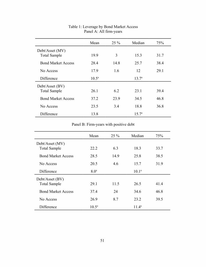
51

Table 1: Leverage by Bond Market AccessPanel A: All firm-years

Mean 25 % Median 75%

Debt/Asset (MV) Total Sample 19.9 3 15.3 31.7

Bond Market Access 28.4 14.8 25.7 38.4

No Access 17.9 1.6 12 29.1

Difference 10.5a 13.7a

Debt/Asset (BV) Total Sample 26.1 6.2 23.1 39.4

Bond Market Access 37.2 23.9 34.5 46.8

No Access 23.5 3.4 18.8 36.8

Difference 13.8 15.7a

Panel B: Firm-years with positive debt

Mean 25 % Median 75%

Debt/Asset (MV) Total Sample 22.2 6.3 18.3 33.7

Bond Market Access 28.5 14.9 25.8 38.5

No Access 20.5 4.6 15.7 31.9

Difference 8.0a 10.1a

Debt/Asset (BV) Total Sample 29.1 11.5 26.5 41.4

Bond Market Access 37.4 24 34.6 46.8

No Access 26.9 8.7 23.2 39.5

Difference 10.5a 11.4a

52

The table reports summary statistics on firms’ total debt ratios by whether they have accessto the public debt markets. We use whether the firm has a debt rating as a measure of whether it hasaccess to the public debt markets. The market value (MV) ratio is total (short- and long-term) debtdivided by the book value of assets minus the book value of equity plus the market value of equity.The book value (BV) debt ratio is debt divided by the book value of assets. The book value ratio isnot always between zero and one; it is above one for 1.3 percent of the sample. We re-coded the bookvalue ratio to one for these observations. The table reports the mean, the 25th, 50th (median), and 75th

percentile in each cell, except for the difference row. This row contains the difference in the means(or medians) and the associated significance levels (a b c denotes statistically significant at the 1%, 5%,and 10% levels). In Panel A there are 77,659 firm-year observations of which 19.0 percent have adebt rating. Panel B contains only firm years in which the firm had a positive amount of debt. InPanel B, there are 69,589 firm-year observations of which 21.1 percent have a debt rating. Thesample is based on firms from Compustat that report sales and assets above $1M between 1986 and2000.

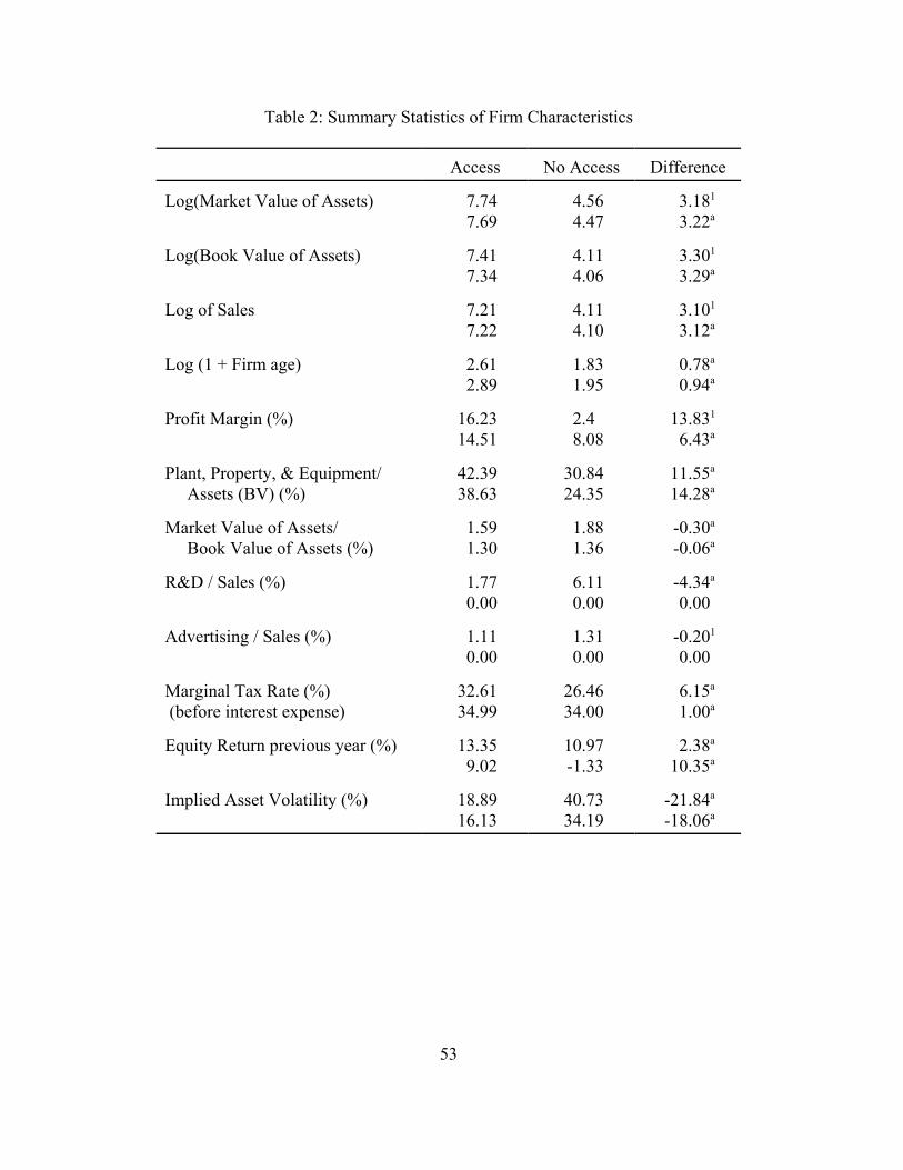
53

Table 2: Summary Statistics of Firm Characteristics

Access No Access Difference

Log(Market Value of Assets)

7.747.69

4.564.47

3.181

3.22a

Log(Book Value of Assets)

7.417.34

4.114.06

3.301

3.29a

Log of Sales

7.217.22

4.114.10

3.101

3.12a

Log (1 + Firm age) 2.612.89

1.831.95

0.78a

0.94a

Profit Margin (%) 16.2314.51

2.48.08

13.831

6.43a

Plant, Property, & Equipment/ Assets (BV) (%)

42.3938.63

30.8424.35

11.55a

14.28a

Market Value of Assets/ Book Value of Assets (%)

1.591.30

1.881.36

-0.30a

-0.06a

R&D / Sales (%) 1.770.00

6.110.00

-4.34a

0.00

Advertising / Sales (%) 1.110.00

1.310.00

-0.201

0.00

Marginal Tax Rate (%) (before interest expense)

32.6134.99

26.4634.00

6.15a

1.00a

Equity Return previous year (%) 13.359.02

10.97-1.33

2.38a

10.35a

Implied Asset Volatility (%) 18.8916.13

40.7334.19

-21.84a

-18.06a

54

The table contains summary statistics for the sample of firms with and without access to thepublic debt markets. Firms that have a debt rating are classified as having access; those without abond rating are classified as having no access. The first number in each cell is the mean; the secondis the median. The third column contains the difference in the means and medians as well as thestatistical significance of the difference. Missing values for R&D and Advertising Expense are setequal to zero. The Market-to-Book Ratio and the Implied Asset Volatility variables are truncated atthe 1st and 99th percentiles. The sample is based on firms from Compustat that report sales and assetsabove $1M between 1986 and 2000 and only includes firm years with debt. a b c Denotes statistically significant at the 1%, 5%, and 10% levels.

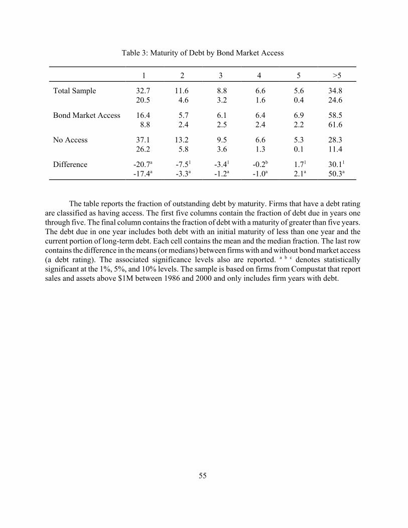
55

Table 3: Maturity of Debt by Bond Market Access

1 2 3 4 5 >5

Total Sample 32.720.5

11.64.6

8.83.2

6.61.6

5.60.4

34.824.6

Bond Market Access 16.48.8

5.72.4

6.12.5

6.42.4

6.92.2

58.561.6

No Access 37.126.2

13.25.8

9.53.6

6.61.3

5.30.1

28.311.4

Difference -20.7a

-17.4a-7.51

-3.3a-3.41

-1.2a-0.2b

-1.0a1.71

2.1a30.11

50.3a

The table reports the fraction of outstanding debt by maturity. Firms that have a debt ratingare classified as having access. The first five columns contain the fraction of debt due in years onethrough five. The final column contains the fraction of debt with a maturity of greater than five years.The debt due in one year includes both debt with an initial maturity of less than one year and thecurrent portion of long-term debt. Each cell contains the mean and the median fraction. The last rowcontains the difference in the means (or medians) between firms with and without bond market access(a debt rating). The associated significance levels also are reported. a b c denotes statisticallysignificant at the 1%, 5%, and 10% levels. The sample is based on firms from Compustat that reportsales and assets above $1M between 1986 and 2000 and only includes firm years with debt.

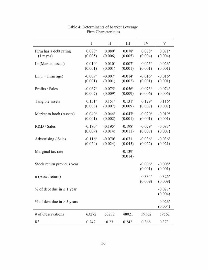
56

Table 4: Determinants of Market Leverage Firm Characteristics

I II III IV V

Firm has a debt rating (1 = yes)

0.083a

(0.005)0.080a

(0.006)0.078a

(0.005)0.078a

(0.004)0.071a

(0.004)

Ln(Market assets) -0.010a

(0.001)-0.010a

(0.001)-0.007a

(0.001)-0.025a

(0.001)-0.026a

(0.001)

Ln(1 + Firm age) -0.007a

(0.001)-0.007a

(0.001)-0.014a

(0.002)-0.016a

(0.001)-0.016a

(0.001)

Profits / Sales -0.067a

(0.007)-0.075a

(0.009)-0.056a

(0.009)-0.073a

(0.006)-0.074a

(0.006)

Tangible assets 0.151a

(0.008)0.151a

(0.007)0.131a

(0.009)0.129a

(0.007)0.116a

(0.007)

Market to book (Assets) -0.040a

(0.001)-0.044a

(0.002)-0.047a

(0.001)-0.020a

(0.001)-0.019a

(0.001)

R&D / Sales -0.180a

(0.009)-0.195a

(0.014)-0.198a

(0.011)-0.079a

(0.007)-0.083a

(0.007)

Advertising / Sales -0.116a

(0.024)-0.070b

(0.024)-0.071(0.045)

-0.036c

(0.022)-0.036c

(0.021)

Marginal tax rate -0.139a

(0.014)

Stock return previous year -0.006a

(0.001)-0.008a

(0.001)

σ (Asset return) -0.334a

(0.009)-0.326a

(0.009)

% of debt due in # 1 year -0.027a

(0.004)

% of debt due in > 5 years 0.026a

(0.004)

# of Observations 63272 63272 48021 59562 59562

R2 0.242 0.23 0.242 0.368 0.373

57

The dependent variable is the ratio of total debt to the market value of the firm’s assets. Whiteheteroscedastic consistent errors, corrected for correlation across observations of a given firm, arereported in parentheses (White, 1980 and Rogers, 1993) except in column II. In column II, thecoefficients and standard errors are estimated using the Fama-MacBeth method (1973). The marketvalue of assets is the book value of assets minus the book value of equity plus the market value ofdebt. All models also include year dummy variables and a dummy variable for the regulated utilityindustry (4900-4939). The sample is based on firms from Compustat that report sales and assetsabove $1M between 1986 and 2000 and only includes firm years with debt. a b c Denotes statistically significant at the 1%, 5%, and 10% levels.

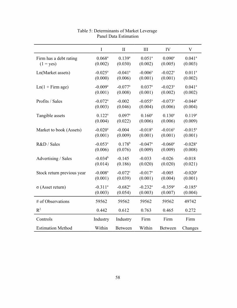
58

Table 5: Determinants of Market Leverage Panel Data Estimation

I II III IV V

Firm has a debt rating (1 = yes)

0.068a

(0.002)0.139a

(0.030)0.051a

(0.002)0.090a

(0.005)0.041a

(0.003)

Ln(Market assets) -0.025a

(0.000)-0.041a

(0.006)-0.006a

(0.001)-0.022a

(0.001)0.011a

(0.002)

Ln(1 + Firm age) -0.009a

(0.001)-0.077a

(0.008)0.037a

(0.001)-0.023a

(0.002)0.041a

(0.002)

Profits / Sales -0.072a

(0.003)-0.002(0.046)

-0.055a

(0.004)-0.073a

(0.006)-0.044a

(0.004)

Tangible assets 0.122a

(0.004)0.097a

(0.022)0.160a

(0.006)0.130a

(0.006)0.119a

(0.009)

Market to book (Assets) -0.020a

(0.001)-0.004(0.009)

-0.018a

(0.001)-0.016a

(0.001)-0.015a

(0.001)

R&D / Sales -0.053a

(0.006)0.178b

(0.076)-0.047a

(0.009)-0.060a

(0.009)-0.028a

(0.008)

Advertising / Sales -0.034b

(0.014)-0.145(0.186)

-0.033(0.020)

-0.026(0.020)

-0.018(0.021)

Stock return previous year -0.008a

(0.001)-0.072c

(0.039)-0.017a

(0.001)-0.005(0.004)

-0.020a

(0.001)

σ (Asset return) -0.311a

(0.003)-0.682a

(0.054)-0.232a

(0.003)-0.359a

(0.007) -0.185a

(0.004)

# of Observations 59562 59562 59562 59562 49742

R2 0.442 0.612 0.763 0.465 0.272

Controls Industry Industry Firm Firm Firm

Estimation Method Within Between Within Between Changes

59

The dependent variable is the ratio of total debt to the market value of the firm’s assets. Themarket value of assets is the book value of assets minus the book value of equity plus the marketvalue of debt. All models also include year dummy variables and a dummy variable for the regulatedutility industry (4900-4939). The sample is based on firms from Compustat that report sales andassets above $1M between 1986 and 2000 and only includes firm years with debt.a b c Denotes statistically significant at the 1%, 5%, and 10% levels.

Column I - Within industry estimates. The coefficients are estimated based on variation of thevariable from the industry specific means. There are 396 distinct 4-digit SIC industry dummies. Thereported R2 includes the explanatory power of the industry dummies. The R2 is 0.288 if we excludethe explanatory power of the industry dummies.Column II - Between industry estimates. The coefficients are estimated based on differences betweenindustry specific means. Column III – Within firm estimates. The coefficients are estimated based on variation of the variablefrom the firm-specific means. There are 9,742 distinct firms. The reported R2 includes the explanatorypower of the firm dummies. The R2 is 0.266 if we do not include the explanatory power of the firmdummies.Column IV – Between firm estimates. The coefficients are estimated based on differences betweenfirm-specific means.Column V – First difference estimates. Estimates are based on the first differences in all variables.

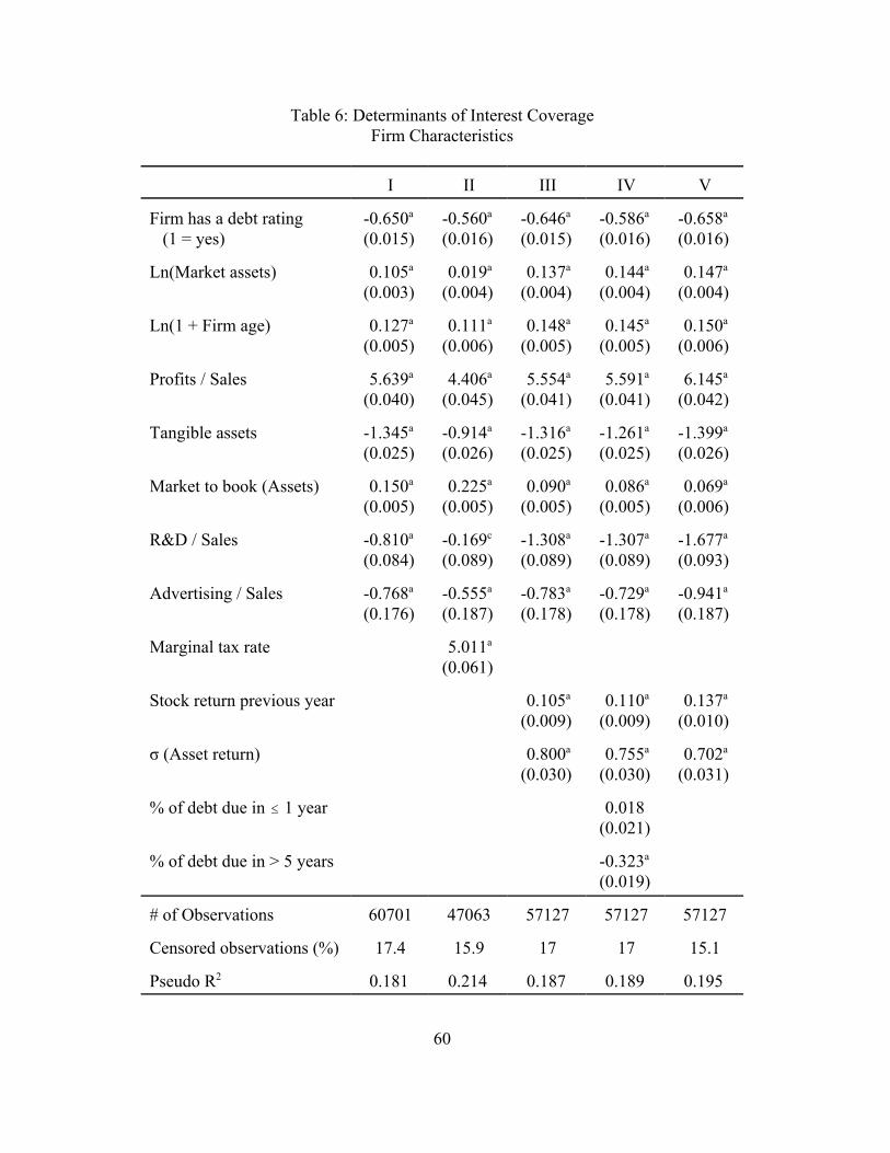
60

Table 6: Determinants of Interest CoverageFirm Characteristics

I II III IV V

Firm has a debt rating (1 = yes)

-0.650a

(0.015)-0.560a

(0.016)-0.646a

(0.015)-0.586a

(0.016)-0.658a

(0.016)

Ln(Market assets) 0.105a

(0.003)0.019a

(0.004)0.137a

(0.004)0.144a

(0.004)0.147a

(0.004)

Ln(1 + Firm age) 0.127a

(0.005)0.111a

(0.006)0.148a

(0.005)0.145a

(0.005)0.150a

(0.006)

Profits / Sales 5.639a

(0.040)4.406a

(0.045)5.554a

(0.041)5.591a

(0.041)6.145a

(0.042)

Tangible assets -1.345a

(0.025)-0.914a

(0.026)-1.316a

(0.025)-1.261a

(0.025)-1.399a

(0.026)

Market to book (Assets) 0.150a

(0.005)0.225a

(0.005)0.090a

(0.005)0.086a

(0.005)0.069a

(0.006)

R&D / Sales -0.810a

(0.084)-0.169c

(0.089)-1.308a

(0.089)-1.307a

(0.089)-1.677a

(0.093)

Advertising / Sales -0.768a

(0.176)-0.555a

(0.187)-0.783a

(0.178)-0.729a

(0.178)-0.941a

(0.187)

Marginal tax rate 5.011a

(0.061)

Stock return previous year 0.105a

(0.009)0.110a

(0.009)0.137a

(0.010)

σ (Asset return) 0.800a

(0.030)0.755a

(0.030)0.702a

(0.031)

% of debt due in # 1 year 0.018(0.021)

% of debt due in > 5 years -0.323a

(0.019)

# of Observations 60701 47063 57127 57127 57127

Censored observations (%) 17.4 15.9 17 17 15.1

Pseudo R2 0.181 0.214 0.187 0.189 0.195

61

The dependent variable is the natural log of one plus the interest coverage ratio. Interestcoverage is operating earnings before depreciation divided by interest expense. The dependentvariable is re-coded to zero for observations with negative earnings; the model is then estimated asa tobit with a lower limit of zero (which corresponds to interest coverage of zero), except in columnV. In column V, we used a lower limit of -0.69 which corresponds to interest coverage of -0.5 [-0.69=ln(1-0.5)]. The percent of observations that are censored also are reported in the table. Whiteheteroscedastic consistent errors, corrected for correlation across observations of a given firm, arereported in parentheses (White, 1980 and Rogers, 1993). All models also include year dummyvariables and a dummy variable for the regulated utility industry (4900-4939). The sample is basedon firms from Compustat that report sales and assets above $1M between 1986 and 2000 and onlyincludes firm years with debt. a b c Denotes statistically significant at the 1%, 5%, and 10% levels.

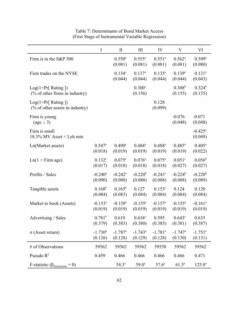
62

Table 7: Determinants of Bond Market Access(First Stage of Instrumental Variable Regression)

I II III IV V VI

Firm is in the S&P 500 0.550a

(0.081)0.555a

(0.081)0.551a

(0.081)0.562a

(0.081)0.599a

(0.080)

Firm trades on the NYSE 0.134a

(0.044)0.137a

(0.044)0.135a

(0.044)0.139a

(0.044)0.121a

(0.043)

Log(1+Pr[ Rating ]) (% of other firms in industry)

0.300c

(0.156)0.308b

(0.155)0.324b

(0.155)

Log(1+Pr[ Rating ]) (% of other assets in industry)

0.128(0.099)

Firm is young (age # 3)

-0.076(0.048)

-0.071(0.048)

Firm is small18.3% MV Asset < Leh min

-0.425a

(0.049)

Ln(Market assets) 0.547a

(0.018)0.490a

(0.019)0.484a

(0.019)0.488a

(0.019)0.485a

(0.019)0.405a

(0.022)

Ln(1 + Firm age) 0.132a

(0.017)0.075a

(0.018)0.076a

(0.018)0.075a

(0.018)0.051c

(0.027)0.056b

(0.027)

Profits / Sales -0.240a

(0.090)-0.242a

(0.088)-0.220b

(0.088)-0.241a

(0.088)-0.224b

(0.088)-0.220b

(0.089)

Tangible assets 0.168b

(0.084)0.165b

(0.083)0.127(0.084)

0.153c

(0.084)0.124

(0.084)0.120

(0.084)

Market to book (Assets) -0.153a

(0.019)-0.158a

(0.019)-0.155a

(0.019)-0.157a

(0.019)-0.155a

(0.019)-0.161a

(0.019)

Advertising / Sales 0.781b

(0.379)0.619

(0.383)0.634c

(0.380)0.595

(0.385)0.643c

(0.381)0.635

(0.387)

σ (Asset return) -1.730a

(0.126)-1.787a

(0.128)-1.743a

(0.129)-1.781a

(0.128)-1.747a

(0.130)-1.751a

(0.131)

# of Observations 59562 59562 59562 59558 59562 59562

Pseudo R2 0.459 0.466 0.466 0.466 0.466 0.471

F-statistic (βInstruments = 0) 54.3a 59.0a 57.6a 61.5a 125.8a

63

The table contains estimates from a probit model where the dependent variable is whether thefirm has a bond rating (access to the public debt markets). Positive coefficients imply that increasesin the variable are associated with a higher probability of a bond rating. White heteroscedasticconsistent errors, corrected for correlation across observations of a given firm, are reported inparentheses (White, 1980 and Rogers, 1993). The Pseudo-R2 is the log-likelihood of the maximumlikelihood minus the log-likelihood when only the constant is included. The instruments are: 1)whether the firm is in the S&P 500 [0 or 1]; 2) whether the firm’s equity trades on the NYSE [0 or1]; 3), log of one plus the percentage of firms in the same 3-digit SIC industry that have a bondrating; 4) log of one plus the percentage of firms in the same 3-digit SIC industry that have a bondrating weighted by the market value of assets; 5) whether the firm’s age is three years or less [0 or1]; and 6) whether the firm’s market value of assets times the median debt ratio (0.183) is less thanthe minimum bond size required to be included in the Lehman Brothers Corporate bond index. Allmodels also include year dummy variables and a dummy variable for the regulated utility industry(4900-4939), as well as the firm’s R&D-to-sales ratio and its stock return over the previous year. Thelast row contains the F-statistic and its significance level for the test that the coefficients on all theinstruments are jointly zero. The sample is based on firms from Compustat that report sales and assetsabove $1M between 1986 and 2000 and only includes firm years with debt.a b c Denotes statistically significant at the 1%, 5%, and 10% levels.

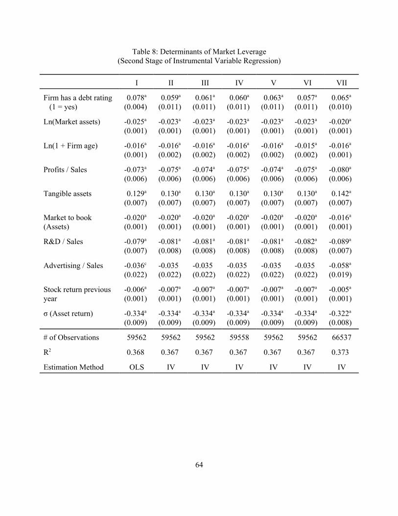
64

Table 8: Determinants of Market Leverage(Second Stage of Instrumental Variable Regression)

I II III IV V VI VII

Firm has a debt rating (1 = yes)

0.078a

(0.004)0.059a

(0.011)0.061a

(0.011)0.060a

(0.011)0.063a

(0.011)0.057a

(0.011)0.065a

(0.010)

Ln(Market assets) -0.025a

(0.001)-0.023a

(0.001)-0.023a

(0.001)-0.023a

(0.001)-0.023a

(0.001)-0.023a

(0.001)-0.020a

(0.001)

Ln(1 + Firm age) -0.016a

(0.001)-0.016a

(0.002)-0.016a

(0.002)-0.016a

(0.002)-0.016a

(0.002)-0.015a

(0.002)-0.016a

(0.001)

Profits / Sales -0.073a

(0.006)-0.075a

(0.006)-0.074a

(0.006)-0.075a

(0.006)-0.074a

(0.006)-0.075a

(0.006)-0.080a

(0.006)

Tangible assets 0.129a

(0.007)0.130a

(0.007)0.130a

(0.007)0.130a

(0.007)0.130a

(0.007)0.130a

(0.007)0.142a

(0.007)

Market to book(Assets)

-0.020a

(0.001)-0.020a

(0.001)-0.020a

(0.001)-0.020a

(0.001)-0.020a

(0.001)-0.020a

(0.001)-0.016a

(0.001)

R&D / Sales -0.079a

(0.007)-0.081a

(0.008)-0.081a

(0.008)-0.081a

(0.008)-0.081a

(0.008)-0.082a

(0.008)-0.089a

(0.007)

Advertising / Sales -0.036c

(0.022)-0.035(0.022)

-0.035(0.022)

-0.035(0.022)

-0.035(0.022)

-0.035(0.022)

-0.058a

(0.019)

Stock return previousyear

-0.006a

(0.001)-0.007a

(0.001)-0.007a

(0.001)-0.007a

(0.001)-0.007a

(0.001)-0.007a

(0.001)-0.005a

(0.001)

σ (Asset return) -0.334a

(0.009)-0.334a

(0.009)-0.334a

(0.009)-0.334a

(0.009)-0.334a

(0.009)-0.334a

(0.009)-0.322a

(0.008)

# of Observations 59562 59562 59562 59558 59562 59562 66537

R2 0.368 0.367 0.367 0.367 0.367 0.367 0.373

Estimation Method OLS IV IV IV IV IV IV

65

The table contains second stage, instrumental variable estimates, except for column I . Incolumn I, the OLS estimates from Table 4, column I are reproduced. The instruments used in eachcolumn (II-VI) are the ones used in the same column of Table 7 (II-VI). In column VII, we use thecoefficients from column VI of Table 7 to predict the probability of having a rating for all firms,not just those with positive debt. We then include the firms with zero debt in the second stage IVestimation. The instruments are: 1) whether the firm is in the S&P 500 [0 or 1]; 2) whether thefirm’s equity trades on the NYSE [0 or 1]; 3), log of one plus the percentage of firms in the same3-digit SIC industry that have a bond rating; 4) log of one plus the percentage of firms in the same3-digit SIC industry that have a bond rating weighted by the market value of assets; 5) whether thefirm’s age is three years or less [0 or 1]; and 6) whether the firm’s market value of assets times themedian debt ratio (0.183) is less than the minimum bond size required to be included in the LehmanBrothers Corporate bond index. White heteroscedastic consistent errors, corrected for correlationacross observations of a given firm, are reported in parentheses (White, 1980 and Rogers, 1993).The sample is based on firms from Compustat that report sales and assets above $1M between 1986and 2000 and only includes firm years with debt, except column VII which also includes firm yearswith zero debt.a b c Denotes statistically significant at the 1%, 5%, and 10% levels.

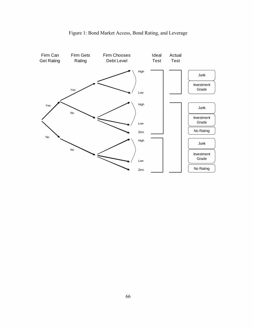
66

Figure 1: Bond Market Access, Bond Rating, and Leverage

Junk

Yes

No

Yes

No

Firm ChoosesDebt Level

Ideal Test

ActualTest

Zero

Zero

InvestmentGrade

Investment Grade

Junk

Junk

Investment Grade

No Rating

No Rating

High

High

High

Low

Low

Low

Firm GetsRating

Firm Can Get Rating

No

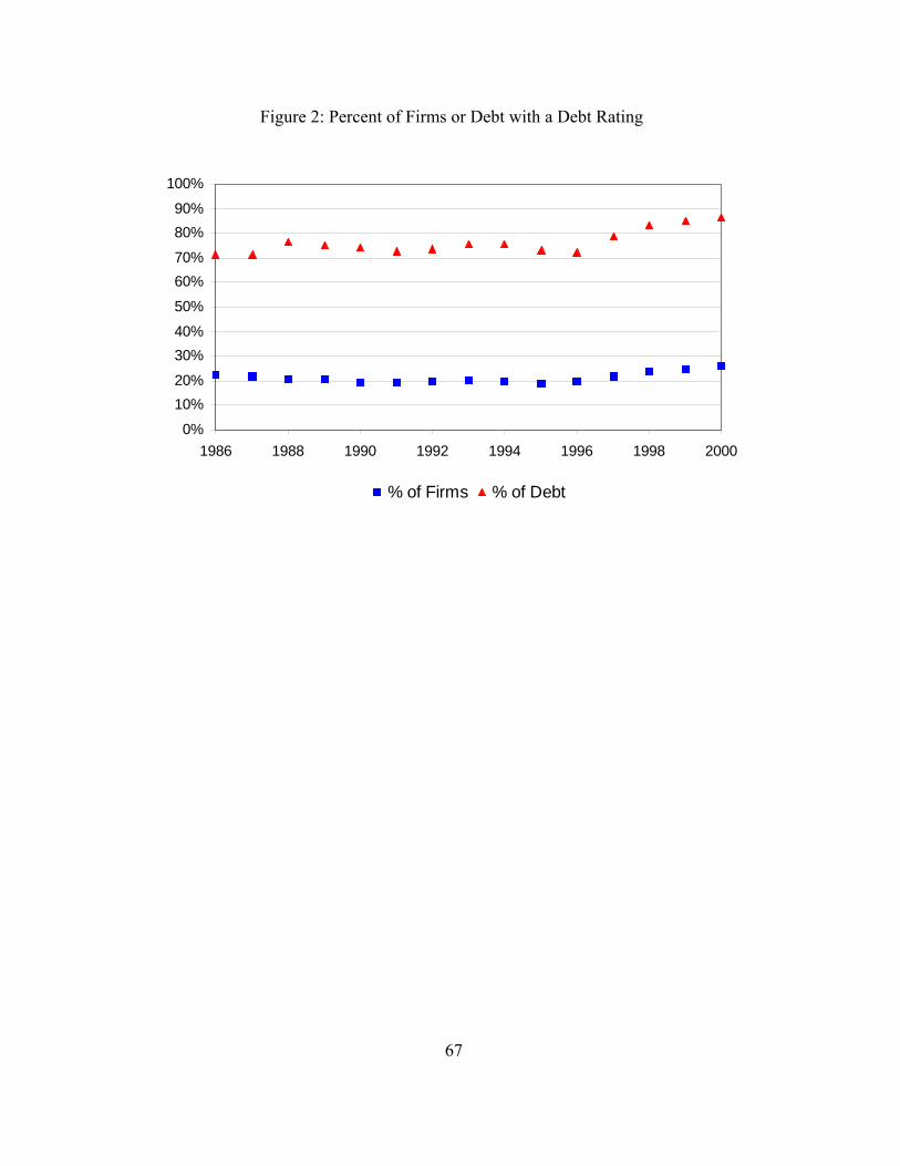
67

Figure 2: Percent of Firms or Debt with a Debt Rating

0%

10%20%

30%40%

50%

60%70%

80%90%

100%

1986 1988 1990 1992 1994 1996 1998 2000

% of Firms % of Debt

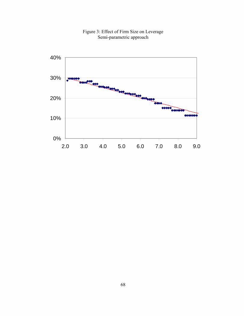
68

Figure 3: Effect of Firm Size on LeverageSemi-parametric approach

0%

10%

20%

30%

40%

2.0 3.0 4.0 5.0 6.0 7.0 8.0 9.0

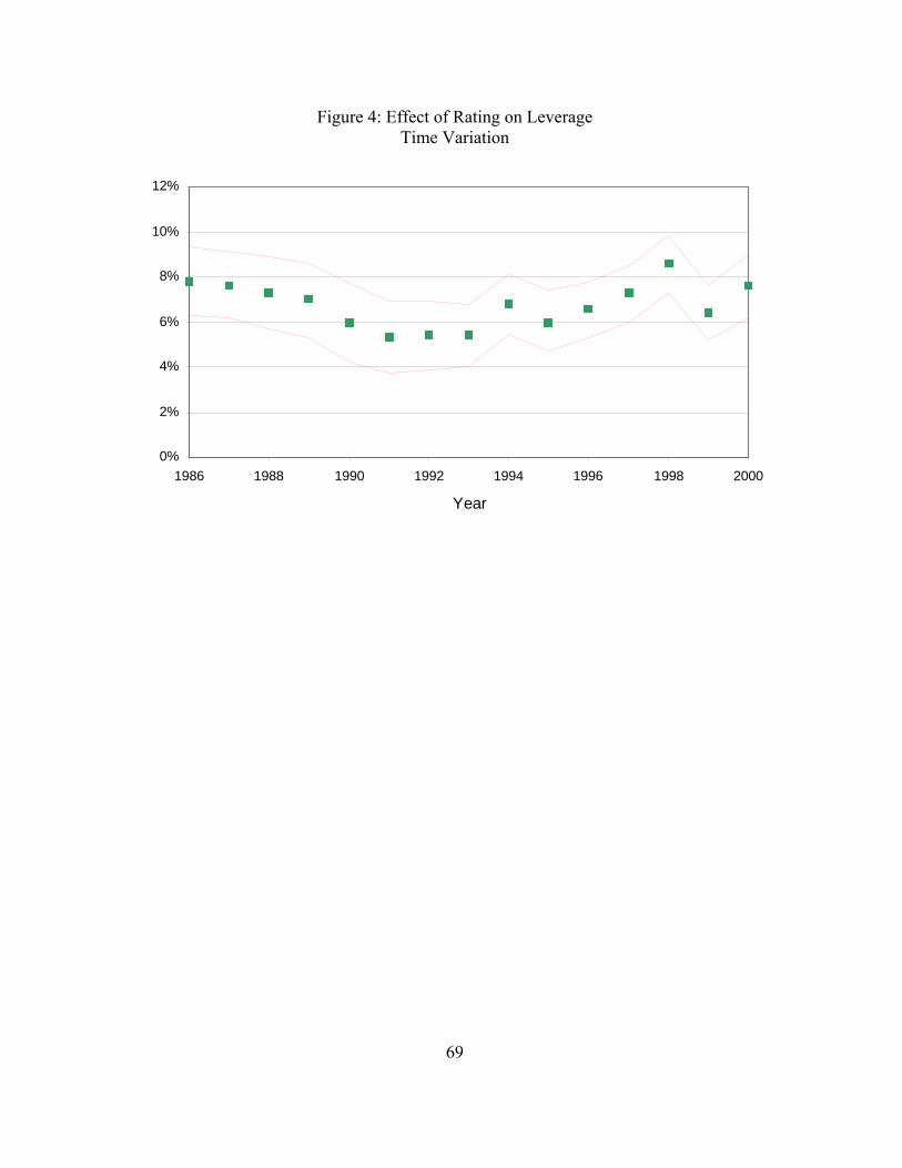
69

Figure 4: Effect of Rating on LeverageTime Variation

0%

2%

4%

6%

8%

10%

12%

1986 1988 1990 1992 1994 1996 1998 2000

Year

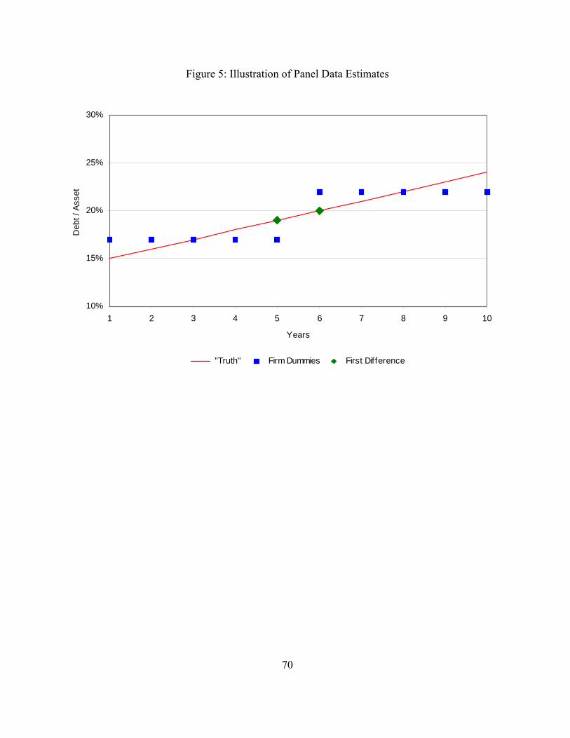
70

Figure 5: Illustration of Panel Data Estimates

10%

15%

20%

25%

30%

1 2 3 4 5 6 7 8 9 10

Years

Deb

t / A

sset

''Truth'' Firm Dummies First Difference