Do Locals Know Better?

A Comparison of the Performance of Local and Foreign

Institutional Investors*

Miguel A. Ferreira

Nova School of Business and Economics

Pedro Matos

University of Virginia - Darden School of Business

João Pedro Pereira†

Nova School of Business and Economics

Pedro Pires

Nova School of Business and Economics

This Version: May 2017

Abstract

We compare the performance of local versus foreign institutional investors using a

comprehensive data set of equity holdings in 32 countries during the 2000-2010 period.

We find that foreign institutions perform as well as local institutions on average, but only

domestic institutions show a trading pattern consistent with an information advantage.

Our results suggest a smart-money effect of local institutions in countries subject to

higher information asymmetry, non-English speaking countries, countries with less

efficient stock markets, with poor investor protection, or high levels of corruption. The

local advantage is more pronounced in periods of market turmoil and in illiquid stocks.

* We are grateful for the helpful comments of Wolfgang Bessler, Geraldo Cerqueiro, Hao Jiang, Ghulame Rubbaniy,

Pedro Saffi, Clemens Sialm, and seminar participants at the Erasmus University Conference on Professional Asset

Management, Luso-Brazilian Finance Meeting, ISCTE Business School - Nova Annual Finance Conference,

Portuguese Finance Network, and Inquire UK and Inquire Europe joint spring seminar. We thank José Caldas for

helping with a mutual fund name matching algorithm in an earlier version of the paper. Financial support from

Inquire Europe is gratefully acknowledged. This work was funded by National Funds through FCT – Fundação para

a Ciência e Tecnologia under the project Ref. UID/ECO/00124/2013 and by POR Lisboa under the project

LISBOA-01-0145-FEDER-007722. † Contact author. Email: joao.pereira@novasbe.pt. Mail: Nova SBE, Universidade Nova de Lisboa, Campus de

Campolide, 1099-032 Lisboa, Portugal. Phone: (+351) 213 801 637.

1

1. Introduction

Financial globalization and the substantial growth of the global mutual fund industry have

expanded investment opportunities for global investors (Khorana, Servaes, and Tufano (2005)).

Investors seeking to allocate money to foreign assets face a choice between investing through an

international, and perhaps sophisticated, money management company or investing through a

local management company, located in the same country as the target securities, and perhaps

with better information about these local securities. Our research aims to shed light on which of

these two investment options is better.

A large literature investigates the effects of geographic distance on investors’ portfolio

decisions and investment performance. Empirical evidence shows that the information

asymmetry that foreign investors face is a determinant of their investment decision (e.g., Gehrig

(1993), Chan, Covrig, and Ng (2005), and Leuz, Lins, and Warnock (2009)), which may help

explain the home-bias phenomenon (French and Poterba (1991), Lewis (1999), and Karolyi and

Stulz (2003)). Home bias may also be the outcome of rational investor choice, whether because

of incentives to hold portfolios similar to those of their neighbors (Cole, Mailath, and Postlewaite

(2001), DeMarzo, Kaniel, and Kremer (2004)) or to make their information set as different as

possible from other investors (Van Nieuwerburgh and Veldkamp (2009)). The preference of

investors for local stocks takes place not only internationally, but also domestically. U.S. money

managers and analysts who are geographically closer to the headquarters of a firm seem to have

an information advantage (Coval and Moskowitz (2001), Malloy (2005), and Baik, Kang, and

Kim (2010)).

Empirical evidence also indicates that local investors outperform foreigners on average:

Shukla and Van Inwegen (1995) in the United States; Hau (2001) in Germany; Choe, Kho, and

2

Stulz (2005) in Korea; Dvorak (2005) in Indonesia; and Teo (2009) in Asia. Local analysts also

seem to have an information advantage over foreign analysts (Bae, Stulz, and Tan (2008)).

Contrary to this local information advantage hypothesis, Albuquerque, Bauer, and Schneider

(2009) develop a theory of equity trading in international markets that is consistent with the idea

that foreign investors have private information that is valuable for trading in many countries

simultaneously. Sophisticated U.S. investors may have a particular advantage in foreign markets

over local investors through global private information that they have acquired in the U.S.

market.

Consistent with this hypothesis, other authors find that foreign investors who participate in a

market can actually be better informed than local investors: Grinblatt and Keloharju (2000) in

Finland; Froot, O’Connell, and Seasholes (2001) in emerging markets; Huang and Shiu (2005) in

Taiwan; Bailey, Mao, and Sirodom (2007) in Singapore and Thailand; and Froot and Ramadorai

(2008) in closed-end funds of 25 countries.

Other authors find no difference between the performance of local and foreign investors:

Kang and Stulz (1997) in Japan, and Seasholes and Zhu (2010) using portfolios of individual

investors. In short, the evidence is mixed on whether local or foreign investors have an

information advantage.

We compare the performance of institutional investors in stocks of their own country

(domestic holdings) to the performance of money managers located in other countries (foreign

holdings). While most of the research to date compares investor performance in a single country,

we use a large sample of institutional money managers in 32 countries over the 2000-2010

period. Using a worldwide sample allows us to get more robust evidence and to provide a more

complete picture of the performance of local and foreign investors around the world.

3

The results show that, on average, domestic and foreign investors perform equally well. The

unconditional average return on domestic portfolios is statistically indistinguishable from the

average return on portfolios of foreign investors. We find that the levels of both types of

institutional ownership – domestic and foreign – have significant forecasting power for one-

quarter-ahead stock returns. This is consistent with the results of Gompers and Metrick (2001),

but extended to a worldwide sample. Furthermore, we find that this effect of both holding types

on future returns comes mostly from a price-pressure effect, rather than from informed trading

by institutional investors.

It would be reasonable to expect, however, that domestic investors would have an

information advantage in more opaque countries, in challenging market conditions, or in specific

stocks in which information asymmetry is likely to be higher. To test these hypotheses, we use

several country-level and stock-level proxies for the quality of a firm’s information environment.

We find indeed an advantage of local institutional investors in shares of firms located in more

opaque countries. When we split the sample on U.S. versus other countries or on English-

speaking countries versus other languages, we find that domestic investors show a more

pronounced information advantage outside the United States and in countries where the official

language is not English (where information asymmetry is likely to be higher). We also find a

local advantage in countries with less efficient stock markets (i.e. stock markets with a lower

share of firm-specific return variation), in countries with weaker investor protection, and in

countries with more corruption. Finally, we find a local advantage during market downturns and

periods of higher aggregate market uncertainty. There is also evidence of a local advantage in

more illiquid stocks.

In summary, the results suggest that only domestic institutions show a trading pattern

4

consistent with an information advantage. When there is high information asymmetry, domestic

investors increase their holdings of a stock before its price goes up, while foreign investors do

not.

2. Methodology

Our first research goal is to analyze the performance difference between domestic and

foreign holdings of institutional investors. We begin with a simple comparison of returns

denominated in U.S. dollars in excess of the U.S. risk-free rate (3-month Treasury Bill rate). We

calculate monthly value-weighted portfolio excess returns on the local and foreign equity

holdings in each market, and then compare the time-series averages of the domestic and foreign

portfolio returns.

To adjust returns for risk using the four-factor Carhart (1997) model, we run a time-series

regression of portfolio returns on either country-specific or global risk factors:

𝑅𝑖,𝑡 = 𝛼𝑖 + 𝛽1,𝑖𝑅𝑀𝑡 + 𝛽2,𝑖𝑆𝑀𝐵𝑡 + 𝛽3,𝑖𝐻𝑀𝐿𝑡 + 𝛽4,𝑖𝑀𝑂𝑀𝑡 + 𝜀𝑖,𝑡 (1)

where 𝑅𝑖,𝑡 is the excess return in U.S. dollars of portfolio i (either the domestic or foreign

portfolio) in month t; 𝑅𝑀𝑡 is the excess return in U.S. dollars on the stock market; 𝑆𝑀𝐵𝑡 (Small

minus Big) is the return on the small capitalization minus the return on the large capitalization

portfolios; 𝐻𝑀𝐿𝑡 (High minus Low) is the return on the high book-to-market minus the return on

the low book-to-market portfolios; and 𝑀𝑂𝑀𝑡 (Momentum) is the return of the past 12-month

winners minus the return on the past 12-month losers portfolios. The global 𝑅𝑀𝑡, 𝑆𝑀𝐵𝑡, 𝐻𝑀𝐿𝑡,

and 𝑀𝑂𝑀𝑡 factors are constructed as value-weighted averages across countries.1

1 The four factors are generated using stock market data from DataStream and WorldScope employing a

methodology similar to that used by Schmidt, Arx, Schrimpf, Wagner, and Ziegler (2015).

5

We first report the alpha from a simple regression on the market factor, and then the alpha

from the full regression on the four factors. In both cases, we are interested in whether the alpha

for the portfolio of domestic holdings is different from the alpha for the portfolio of foreign

holdings.

Next, we study the difference in predictive power between domestic and foreign institutional

ownership using multiple regressions. Following Gompers and Metrick (2001) and Baik, Kang

and Kim (2010), we run a regression of one-quarter-ahead stock returns (𝑅𝑖,𝑡+1) on the current

levels of domestic and foreign institutional ownership:

𝑅𝑖,𝑡+1 = 𝛽1𝐼𝑂𝑖,𝑡𝐷𝑜𝑚 + 𝛽2𝐼𝑂𝑖,𝑡

𝐹𝑜𝑟 + 𝛾1𝑋𝑖,𝑡 + 𝛾2𝐷𝑢𝑚𝑚𝑖𝑒𝑠𝑖,𝑡 + 𝜀𝑖,𝑡 (2)

where X includes several variables known to influence returns, and the dummies control for

industry, country, and time patterns. A higher coefficient on 𝐼𝑂 for a type of investor suggests

the flows of this group of investors predict stock returns better.

There are two explanations for why a group of investors’ flows may predict stock returns.

The first, which is known in the literature as the price-pressure explanation, is that investors can

generate movements in equity returns that are unrelated to underlying fundamentals. In models

such as Frankel and Froot (1987), DeLong, Shleifer, Summers, and Waldmann (1990), Barberis

and Shleifer (2003), and Hong and Stein (2003), the similar, even if uninformed, trading pattern

of a group of investors (e.g., positive feedback trading) temporarily soaks up the available

liquidity for an asset. The asset price may move away from its fundamental value and this

uninformed trading pattern persists until additional liquidity arrives. The second, which is known

as the information explanation, is that one group of investors is more informed than other

investors. This group of investors perceives relevant fundamentals better than other investors,

and engages in purchases or sales when they anticipate movements in these fundamentals. When

6

fundamentals are later revealed, equity prices adjust to their new level.

To understand the source of the local or foreign advantage, we employ the methodology of

Gompers and Metrick (2001) and Baik, Kang, and Kim (2010). Specifically, we decompose total

institutional ownership (𝐼𝑂𝑖,𝑡) into last period’s level (𝐼𝑂𝑖,𝑡−1) plus the change from last period to

this period (Δ𝐼𝑂𝑖,𝑡). We then regress future returns on these variables:

𝑅𝑖,𝑡+1 = 𝛽1𝐼𝑂𝑖,𝑡−1𝐷𝑜𝑚 + 𝛽2Δ𝐼𝑂𝑖,𝑡

𝐷𝑜𝑚 + 𝛽3𝐼𝑂𝑖,𝑡−1𝐹𝑜𝑟 + 𝛽4Δ𝐼𝑂𝑖,𝑡

𝐹𝑜𝑟

+𝛾1𝐶𝑜𝑛𝑡𝑟𝑜𝑙𝑠𝑖,𝑡 + 𝛾2𝐷𝑢𝑚𝑚𝑖𝑒𝑠𝑖,𝑡 + 𝜀𝑖,𝑡 (3)

According to Gompers and Metrick (2001), if the relation between institutional ownership

and returns is driven by a demand-shock or price-pressure explanation, the lagged level of

institutional ownership (𝐼𝑂𝑖,𝑡−1) should forecast returns better than the change (Δ𝐼𝑂𝑖,𝑡) does. The

assumption is that the lagged level of institutional ownership (𝐼𝑂𝑖,𝑡−1) is a good predictor of

future institutional demand because institutional demand patterns are relatively stable over time.

On the other hand, if the relation between IO and returns is driven instead by an information or

smart-institutions explanation, the recent shift in institutional holdings, captured by Δ𝐼𝑂𝑖,𝑡,

should forecast returns better than 𝐼𝑂𝑖,𝑡−1 does. In summary, the Gompers and Metrick (2001)

argument is that a positive coefficient on the lagged level suggests a price-pressure explanation,

while a positive coefficient on the first difference suggests an information explanation.

Given the literature, it is not clear whether we should expect any unconditional aggregate

performance difference between domestic and foreign investors. Nevertheless, we expect

domestic investors to perform better in countries, market conditions, and stocks in which

information asymmetry is likely to be higher. To test this hypothesis, we split the sample using

several country-level and stock-level proxies for the quality of the firm’s information

environment. We then run the same regression for each separate subsample and check whether

7

the domestic holdings have stronger predictive ability in high information asymmetry

environments.

3. Data and variable construction

3.1. Sample

Our sample combines several data sources. We first collect a list of all firms covered in the

Datastream/WorldScope database for 32 countries. We also collect a set of characteristics for

each firm and for its stock market from Datastream/WorldScope.

Institutions defined as professional money managers with discretionary control over assets

(such as mutual funds, pension funds, bank trusts, and insurance companies) are frequently

required to disclose their holdings publicly. We obtain historical filings from the

FactSet/LionShares database from January 2000 through December 2010 on a quarterly basis.

FactSet/LionShares is a leading source for institutional equity holdings worldwide. The data

sources are public filings by investors, such as Securities and Exchange Commission (SEC) 13-F

filings (fund family level) and N-SAR (individual fund level) in the United States. For equities

traded outside the United States, FactSet/LionShares collects ownership data directly from

sources such as national regulatory agencies or stock exchange announcements, mutual fund

industry directories, and company proxies and annual reports. Ferreira and Matos (2008) use this

data set to study the role of institutional investors in corporations around the world. Following

Gompers and Metrick (2001), we set institutional ownership variables to zero if a stock is not

held by any institution in FactSet/LionShares.

We extract the number of analysts following a stock from the IBES database. The list of

MSCI components is obtained from the Bloomberg Financial Services database. Country-level

8

variables are obtained from the World Bank collection of development indicators database. The

Chicago Board Options Exchange (CBOE) volatility index (VXO series) is obtained from the

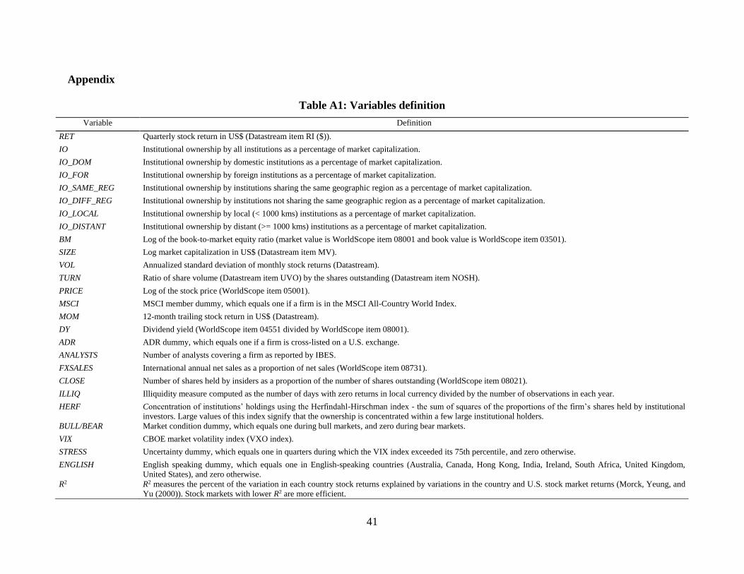
CBOE website. Our final sample covers 632,505 firm-quarters. Table A1 in the Appendix

provides variable definitions and data sources.

3.2. Classifying domestic versus foreign holdings

We first define total institutional ownership (IO) as the sum of the holdings of all institutions in a

firm’s stock divided by market capitalization at the end of each calendar quarter. We sum

institutional positions in both local and American Depositary Receipts (ADR) shares.

For each stock, we compute the holdings of investors based on the country of the institution

that holds a position in the stock. We classify an institutional holding as domestic when the

stock’s country equals the institution’s country. We classify an institutional holding as foreign

when the stock’s country does not equal the institution’s country. We consider as a stock’s

country the country where the company is domiciled according to the Datastream/Worldscope

database. We consider as an institution’s country the country where the investment company is

domiciled according to the FactSet/LionShares database.

We also explore alternative classifications of institutional holdings. First, we divide each

institution’s portfolio into a same region and different region portion, using the geographic

region (Africa, Asia, Eastern Europe, Japan, Latin America, North America, Oceania, and

Western Europe) of the institution and of the stock. We classify an institutional holding as same

region when an institution is located in the same region where the stock is domiciled. We

classify an institutional holding as different region when an institution is located in a different

region from the one where the stock is domiciled.

Finally, we divide each institution’s portfolio into a local and distant portion, using the

9

distance between the institution and the stock as in Coval and Moskowitz (2001). More

specifically, we classify an institutional holding as local when an institution’s country is less than

1,000 kilometers away from the stock’s country (distance measured as the distance between

capital cities). We classify an institutional holding as distant when an institution’s country is

more than 1,000 kilometers away from the stock’s country.

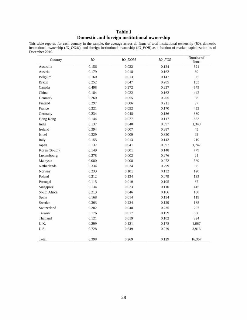
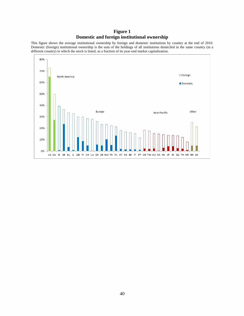
Table 1 presents domestic versus foreign institutional holdings as a percentage of market

capitalization in each country as of December 2010. Figure 1 shows that the prevalence of

foreign and domestic institutional money managers varies considerably across countries.

Domestic investors hold large fractions of the market in the United States, Canada, and Sweden,

but foreign institutions actually hold the largest fraction of local market capitalization in

countries like Australia, France, Germany, Netherlands, and Switzerland.

3.3. Proxies for information asymmetry

We investigate whether the relation between stock returns and institutional holdings depends on

the level of information asymmetry between investors. We use several proxies for information

asymmetry commonly employed in the academic literature.

We start by examining information asymmetry at the country level. We split countries

according to the levels of the following variables: stock market efficiency (using the R2 of

Morck, Yeung, and Yu (2000)); a corruption index (La Porta, Lopez-de-Silanes, Shleifer, and

Vishny (1998)); an index of financial disclosure (Jin and Myers, 2006); and an index of anti-

director rights or shareholder protection (La Porta, Lopez-de-Silanes, Shleifer, and Vishny

(1998)). Additionally, we also split countries by geographic region (U.S. vs. other countries) and

language (English speaking vs. non-English speaking countries). Table A1 in the appendix

provides details on the construction and interpretation of each variable.

10

Next, we consider information asymmetry due to different market conditions. Consistent

with the idea that information asymmetry is greater during worse economic conditions, we split

the sample according to different market cycles. The periods 2000:Q1-2002:Q2 and 2008:Q1-

2009:Q1 are classified as bear market periods, while other periods are classified as bull market

periods. Additionally, we also split the sample into periods of high or low market uncertainty.

We define a period of high market uncertainty, or stress, when the VIX is above its 75th

percentile.

Last, we focus on stock-specific characteristics that may proxy for information opaqueness at

the firm level. Our first proxy is the number of analysts covering the stock. Coverage by analysts

can significantly reduce any information gap between local and foreign institutions. Second, we

split the sample according to the volatility of the stock. In stocks with higher volatility there is

more room for exploitable trading opportunities due to information asymmetry. Third, we

include stock illiquidity, measuring illiquidity by the percentage of days with zero stock returns,

as illiquidity is positively related to information asymmetry.

We also analyze how performance changes with the ownership structure of the firm. In firms

with high insider ownership and high Herfindahl index of ownership concentration, there are

more private benefits of control, and managers will have fewer incentives to seek transparency.

We also include other firm-level proxies. One of these proxies is firm size, measured by the

firm’s market capitalization in U.S. dollars, as larger firms are usually considered to have lower

information asymmetry than smaller firms. We also include the book-to-market ratio (B/M) since

previous empirical literature documents that high-uncertainty firms are more likely to be growth

firms (Zhang, 2006).

11

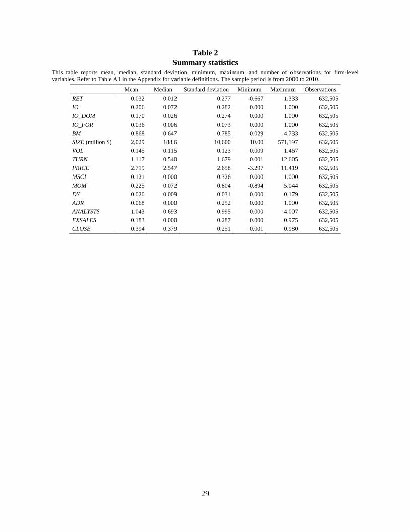
3.4. Descriptive statistics

Table 2 provides summary statistics on stock returns, institutional ownership variables, and firm-

level control variables. Table A1 in the Appendix provides variable definitions and data sources.

Stock returns, volatility, turnover, share prices, and financial ratios are winsorized at the bottom

and top 1%.

We find that the mean institutional ownership is 20.6%, with a median of 7.2%. The mean

foreign ownership is small compared to the mean local ownership, 3.6% versus 17%. The mean

one-quarter-ahead stock return is 3.2%. The mean book-to-market ratio is 0.87. The mean

(median) market capitalization is $2.03 billion ($188.6 million). Stock return volatility is 14.5%,

and turnover is 1.1, on average. The MSCI membership dummy shows that about 12% of our

sample firms are included in the MSCI All Country World Index. Mean and median dividend

yields are close to 2% and 1%, respectively. The ADR dummy shows that about 7% of our

sample firms are cross-listed on a U.S. exchange. On average, our sample firms have one analyst

following the stock. Finally, foreign sales are 18% of total sales, and closely held shares are 39%

of shares outstanding.

4. Empirical results

4.1. Average performance of domestic and foreign portfolios

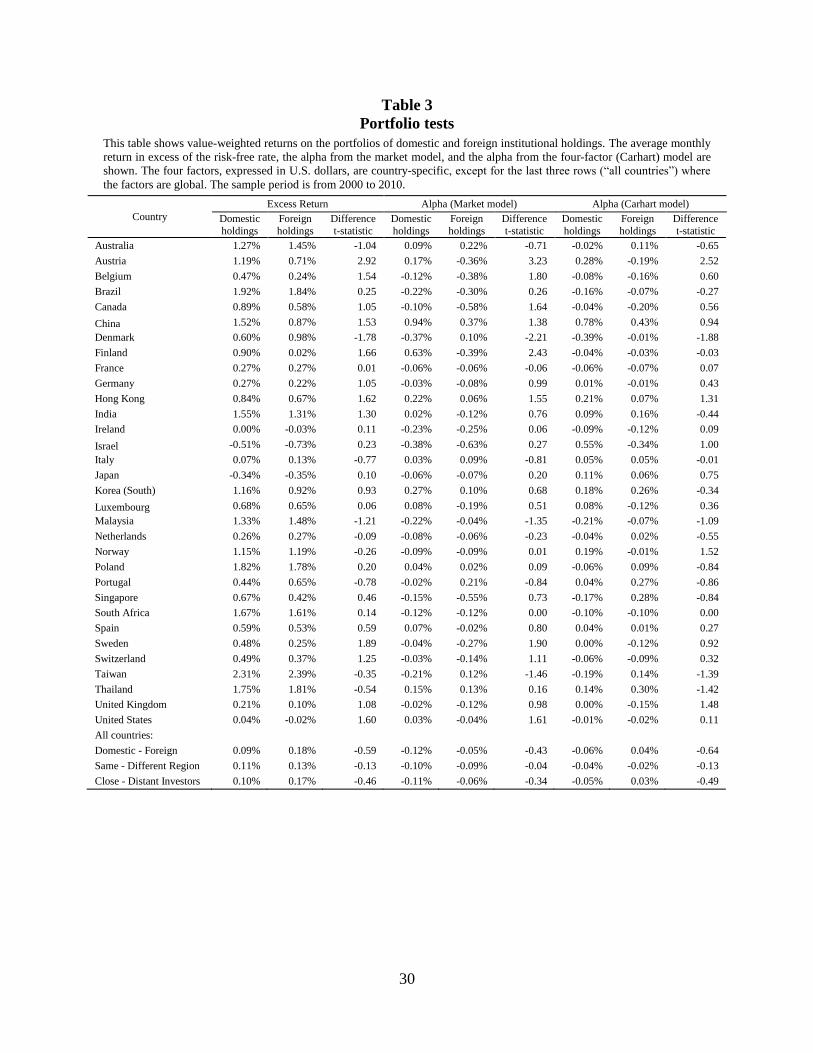
Table 3 presents the time-series average of monthly excess returns of domestic and foreign

institutional portfolios for each country in the sample. For example, in the row for Australia, the

domestic return represents the value-weighted average return of all Australian shares held by

Australian investors, while the foreign return represents the value-weighted average return of all

Australian shares held by investors located outside Australia. Our focus is on the difference

12

between the returns of these two groups.

As the average excess returns of domestic and foreign holdings are similar, we cannot reject

the hypothesis of equality of average excess returns at conventional significance levels in almost

every country. Computing a global average excess return across all domestic and all foreign

holdings, we find that domestic holdings earn an average return of 0.09% per month, while

foreign holdings earn an average return of 0.18% per month. Overall, the difference in average

returns is not statistically significant.

This lack of statistical difference is confirmed when we use risk-adjusted returns. The alphas

from a country-specific market model and the alphas from a country-specific four-factor model

consistently show that the average performance of domestic investors is statistically similar to

the performance of foreign investors.2

To verify that these results do not depend on our domestic and foreign institution

classifications, the last two rows of the table show global average returns according to alternative

classifications of holdings from the same versus different geographic region and from close

versus distant investors.3 Once again, we find that the performance of the two groups of investors

is not significantly different.

We find overall that domestic and foreign holdings of institutional investors earn similar

average stock returns. However, this unconditional average may mask significant differences in

specific stocks or market conditions. We explore this possibility in the following sections.

4.2. Predictive power of domestic and foreign institutions

In this section, we examine how future stock returns are related to total, local, and foreign

2 We find qualitatively similar results if we (1) use global factors, (2) exclude U.S. investors or (3) use local

currencies (see Tables IA.1, IA.2, and IA.3 of the internet appendix, respectively). 3 The results at the country level are available in Table IA.4 of the internet appendix.

13

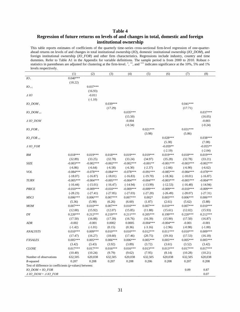
institutional ownership using a multiple regression framework. We expand the Gompers and

Metrick (2001) analysis of U.S. stocks to a worldwide panel with firms from 32 countries. Table

4 presents the results of regressing future quarterly stock returns on institutional ownership, as

well as several control variables.

First, we find that the level of total institutional ownership predicts one-quarter-ahead stock

returns (column (1)). To further analyze this result, we follow Gompers and Metrick (2001) and

Baik, Kang, and Kim (2010), and use the level of lagged institutional ownership as a measure of

future institutional demand and the change in institutional ownership as a measure of

institutional information advantage. The results in column (2) show that the coefficient on lagged

institutional ownership is significantly positive, while the change in institutional ownership is not

statistically significant. This suggests that institutional flows predict future stock returns due to a

demand shock explanation, rather than an information advantage, which is in line with the results

in Gompers and Metrick (2001).4

Next, we compare how domestic and foreign holdings of institutional investors forecast stock

returns. The holdings are classified into domestic or foreign according to the nationality of the

domicile of the institution and of the stock. The results in columns (3) and (5) in table 4 show

that domestic and foreign holdings independently have a positive relation with future stock

returns. When we include both holdings in the same regression (column 7), the coefficients show

that a 10 percentage point increase in domestic institutional ownership increases one-quarter-

ahead returns by 0.4%, while the effect is only slightly lower for foreign institutional ownership

at 0.3%. To compare both coefficients, we run an F-test for the equality of coefficients on local

4 Wermers, Yao, and Zhao (2012) show that portfolio holdings of U.S. mutual funds are useful in predicting

stock returns, provided that the holdings are weighted by the estimated skill level of each fund manager. Our results

are complementary to theirs, in the sense that we study a larger sample of countries and institutional investors, while

doing a simpler aggregation of portfolio holdings. While their results are consistent with some funds possessing

superior skills, the results in this section suggest that the “average” fund exerts mostly a price-pressure effect.

14

and foreign institutional ownership. We cannot reject the null of equal coefficients at the 5%

significance level. Therefore, using a worldwide sample, we conclude that neither domestic

investors nor foreign investors have a return predictive edge.

To disentangle the smart institutions and demand shock explanations, we also run a

specification with the level of and changes in domestic and foreign institutional ownership

(columns (4), (6), and (8)). Lagged institutional ownership is positive for both domestic and

foreign holdings, consistent with a demand shock effect. Furthermore, we find that foreign

institutions seem to be at a slight information disadvantage. While an increase in foreign

holdings is associated with a reduction in future stock returns, a change in local holdings is not

statistically related to future returns.

We find further evidence for the price-pressure hypothesis from additional tests shown in

Table IA.5 of the Internet Appendix. First, we separate countries with high total institutional

ownership from countries with low total institutional ownership. There should be more price

pressure in the former group. Indeed, we find that the coefficients on the level of institutional

holdings are much stronger in countries with high IO than in countries with low IO.

Second, given that the net inflow of money into institutions decreases substantially after 2005

(values not shown, but available upon request), we split the sample into two subperiods: 2000-

2005 and 2006-2010. The results show that the coefficient on the level of foreign institutional

ownership becomes statistically insignificant after 2005, when smaller inflows lead to less

demand pressure. We find, however, that the coefficient on the level of domestic ownership

remains statistically significant in the second period. To investigate this result, we further split

the later-period sample into low versus high domestic inflow countries, that is, countries that

have on average negative domestic inflows versus countries that have on average positive

15

domestic inflows. We find that the level of domestic institutional ownership is significant only

for the group with high inflows, consistent with a price-pressure effect. However, the U.S.

behave differently: even though they have low domestic inflows during 2006-2010, the

coefficient on domestic IO remains positive. This may be explained by the U.S. being, by far, the

country with the highest level of domestic ownership (recall figure 1). Even without more

inflows, just the rebalancing of very large domestic portfolios may sustain the observed price-

pressure effect.

To summarize, our results generalize to a worldwide basis the finding of Gompers and

Metrick (2001) for the U.S. market. We find that the unconditional forecasting power of

institutional ownership for stock returns comes from a demand shock effect, not from a smart

institutions effect.

The presence of demand pressure effects has different implications for individual investors

depending on their investment horizons and holding periods. Shorter-term investors may benefit

from higher returns when they initiate and liquidate their portfolios during periods of growth in

aggregate institutional holdings. In contrast, longer-term investors may see comparatively lower

returns if there is a reduction in flows to institutional investors before their horizon. Foreign

investors typically have shorter horizons than domestic investors so they are more likely to

benefit from demand pressure effects.

4.3. Alternative explanations

It could be the case that lagged institutional ownership is not simply an indicator of price

pressure. Specifically, institutional investors could exploit the underreaction of market

participants to cash flow news by increasing their positions in these undervalued stocks only

slowly over time (Cohen, Gompers, and Vuolteenaho (2002)). Under this interpretation, a high

16

lagged institutional ownership signals the ability of institutional investors to detect mispricing

which can be perceived as superior abilities. To verify whether the results from the Gompers and

Metrick (2001) framework could be driven by this alternative explanation, we implement

additional tests to better support our baseline results.

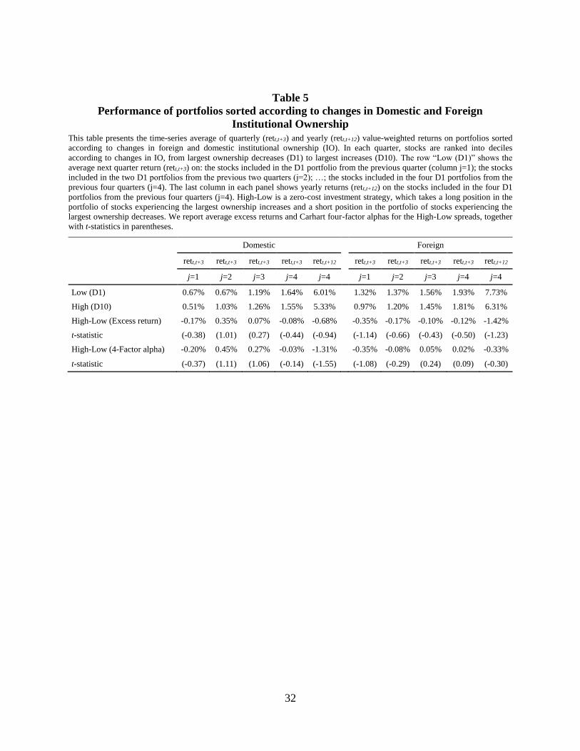
In order to detect any information advantage that is only revealed slowly through time, we

analyze the return on portfolios formed on institutional buys and sales up to four quarters ago.

The procedure is as follows. First, stocks are ranked in each quarter into deciles according to

changes in institutional ownership, from largest ownership decreases (decile 1) to largest

increases (decile 10). At any point in time there are j portfolios with a given decile ranking, with

each portfolio being formed over one of the prior j quarters. We combine these j portfolios into a

single equal-weighted portfolio and hold it during the next quarter. Then, we also compute a

zero-cost portfolio that goes long on the stocks in the tenth decile (“strong” buys) of institutional

ownership variation and goes short on the stocks in the first decile (“heavy” sales). Additionally,

in order to provide a summary measure of performance over several quarters, we also compute

the one-year-ahead performance of portfolios formed on the deciles of institutional trades over

the previous four quarters. This portfolio formation procedure is similar to the overlapping

momentum portfolio procedure of Jegadeesh and Titman (1993).

The results are reported in Table 5. We find that the performance of the high-ownership

portfolio is very similar to the low-ownership portfolio. In fact, the one-quarter return on a long-

short portfolio is not statistically different from zero. This is true for returns from portfolios

formed from institutional trades one quarter ago through four quarters ago. Furthermore, the

long-short one-year-ahead return is also statistically indistinguishable from zero. These results

hold for both domestic and foreign investors, and do not depend on whether we use simple

17

excess returns or four-factor risk adjusted returns. In summary, these results suggest that

institutional trades on average are uninformed, which is supportive of the price-pressure

hypothesis.

Additionally, our results are consistent with the possibility that some institutional investors in

our sample may be herding (as in Brown, Wei, and Wermers (2014)). Herding would reflect

trading on commonly available information, rather than skill of specific institutional investors,

and would contribute to the price-pressure effect that we find.

Finally, our distinction between domestic and foreign investors might be affected by foreign

institutions outsourcing fund management to local managers. However, Chuprinin, Massa, and

Schumacher (2015) find that only 23.9% of mutual funds are outsourced, and from those only

19.7% are outsourced to a management company from a different country. Therefore, it does not

seem likely that our results could be significantly affected by cross-border outsourcing.

4.4. Predictive power of institutional investors under information asymmetry

While the results above fail to reveal any significant advantage of either domestic or foreign

investors, previous research suggests that local and foreign investors may perform differently in

markets or stocks with different levels of information asymmetry (Baik, Kang, and Kim (2010)).

Therefore, we use our broad panel of 32 countries to investigate further the relation between

future stock returns and institutional holdings conditioning on different country and stock

characteristics that may reflect information asymmetry or opaqueness.

To test whether the level of information asymmetry influences the predictive power of local

and foreign institutions, we first divide stocks into those with high information asymmetry and

those with low information asymmetry, and then run a regression of future returns on the level of

and changes in domestic and foreign institutional ownership (and other firm- and country-level

18

controls). A positive coefficient on the level of ownership suggests a price pressure or demand

shock effect, while a positive coefficient on the change in ownership suggests an information or

smart institutions effect.

We start by testing the effect of information asymmetry at the country level. Given that

information asymmetry is a hard-to-measure concept, we consider several alternative proxies in

turn: U.S. versus non-U.S. countries; English-speaking countries versus other languages; a

corruption index (La Porta, Lopez-de-Silanes, Shleifer, and Vishny (1998)); an index of financial

disclosure (Jin and Myers, 2006); an index of anti-director rights or shareholder protection (La

Porta, Lopez-de-Silanes, Shleifer, and Vishny (1998)); and the average R2 of an international

market model as a measure of functional efficiency (Morck, Yeung, and Yu (2000)). Table A1 in

the appendix provides details on the construction and interpretation of each variable.

We begin by examining how the predictive power of local and foreign holdings varies

according to characteristics of the country where the firm is located. We consider several

alternative proxies for information asymmetry: U.S. versus non-U.S. countries; English-speaking

countries versus other languages; a corruption index; an index of financial disclosure; an index of

anti-director rights or shareholder protection; and the average R2 of an international market

model as a measure of functional efficiency (Morck, Yeung, and Yu (2000)).5

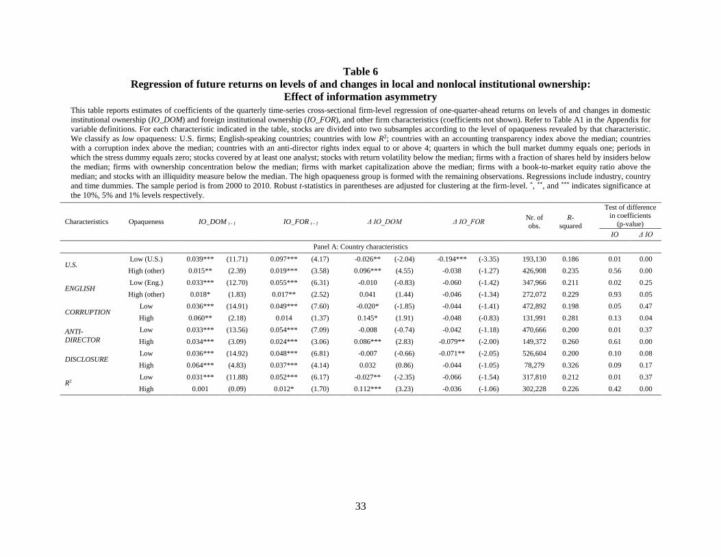
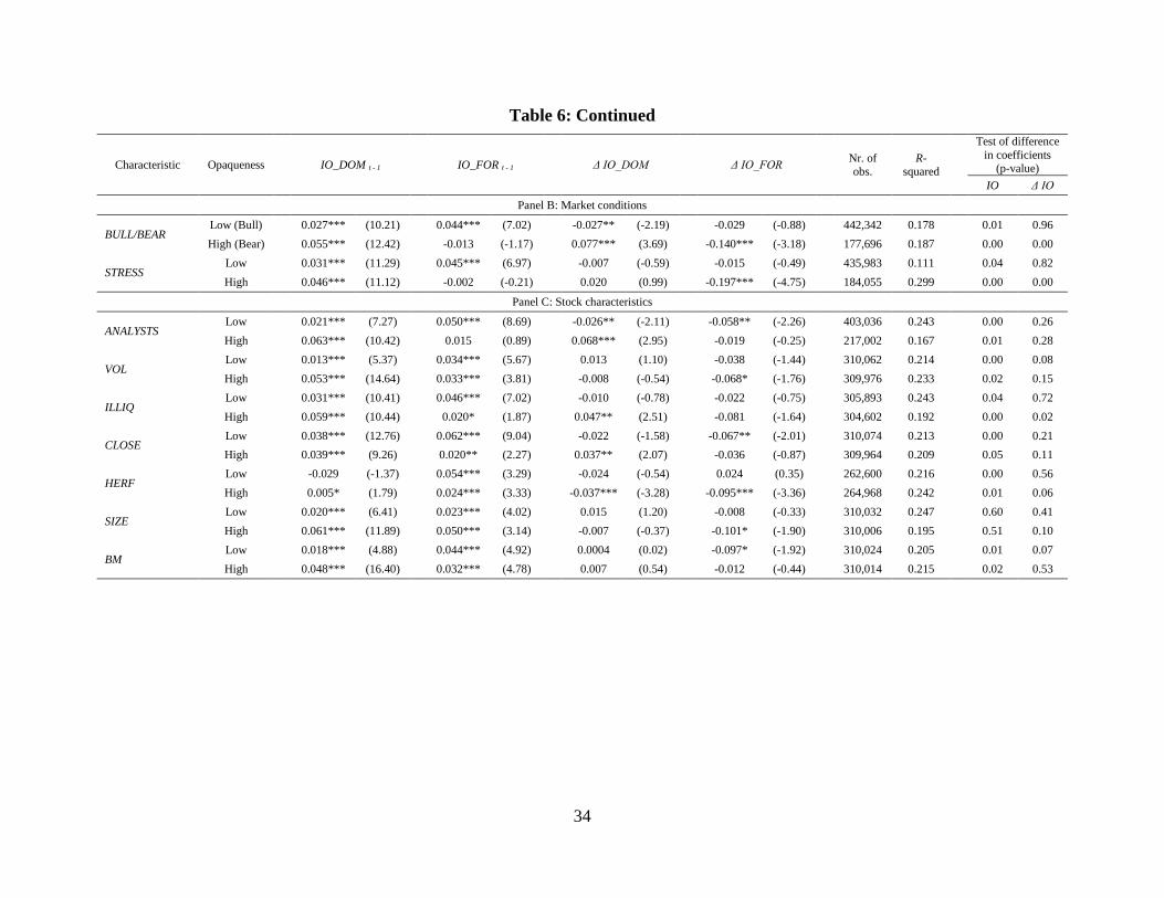
Table 6 shows the results. For each country characteristic in Panel A, there are two

subsamples, according to whether the level of the characteristic indicates high or low information

opaqueness (as defined in Table A1). We find that the coefficients on the lagged level of

ownership are significantly positive for both domestic and foreign institutions in almost every

sample split. This indicates that, whatever the country information environment, institutions have

a strong price pressure effect, which is consistent with our previous results.

5 Table A1 in the Appendix provides details on the construction of each variable.

19

More important, we now find evidence of a domestic smart money effect in several cases

where there is likely to be higher information opaqueness or asymmetry. In particular, we find

that domestic investors on average seem to trade with an information advantage in the following

cases: in countries with high levels of corruption; in countries with weak investor protection (i.e.,

with few anti-director measures); in countries with less efficient stock markets; in countries

outside the U.S.; or in countries where the official language is not English. In all these cases

where information asymmetry is likely to be more severe, increases in the holdings of domestic

investors are followed by higher future returns, while increases in holdings of foreign investors

are followed by lower stock returns.

Next, we explore a different dimension of information asymmetry, namely we look at

institutional performance during periods with different market conditions. We assume that there

is more information opaqueness during stock market downturns (bear markets) or during periods

with high market volatility (stress periods). The results in Panel B of Table 6 show a

disadvantage for foreign investors under high information asymmetry. More precisely, during

bear markets or during periods of higher market uncertainty, foreign investors rebalance their

portfolios in the wrong direction, that is, an increase in their holdings is followed by lower stock

returns. Domestic investors, though, are able to trade in the right direction during bear markets,

and they exert higher price pressure during both bear markets and high-volatility periods.

Finally, we explore information asymmetry at the stock level by splitting the sample

according to several firm-level characteristics that may proxy for opaqueness, as detailed in

Panel C of Table 6. We find a statistically significant information advantage of domestic

investors in illiquid stocks, which are likely to be more opaque. Other characteristics provide less

strong evidence for a smart-money effect of domestic institutions. Domestic institutions trade in

20

the right direction in stocks with low analyst coverage and high inside ownership stocks, while

foreign institutions do not, but the difference between the coefficients is not statistically

significant. Nevertheless, domestic investors exert significantly higher price pressure on stocks

with low analyst coverage (high information opaqueness), high volatility (high opaqueness), high

fractions of outstanding shares held by insiders (high opaqueness), and on stocks with low book-

to-market (high opaqueness).

Overall, our results from a global sample of 32 countries show that domestic institutions

trade with an information advantage over foreign institutions in more opaque countries, during

market periods in which information asymmetry is likely to be higher, and in illiquid stocks.

5. Robustness

5.1. Alternative institutional ownership classifications

Our main results use a classification of domestic or foreign holdings according to the nationality

of the institution versus the nationality of the stock. We now check whether the results are robust

to alternative classifications.

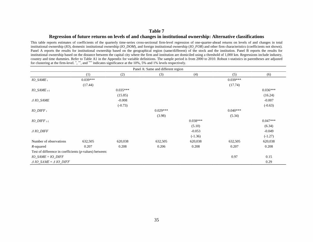
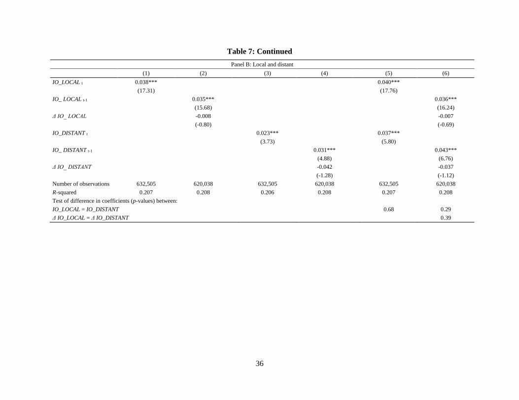
First, we consider a coarser criterion of geographic region instead of country, and split

holdings into same region and different region (Panel A of table 7). Second, we measure

proximity by the actual geographical distance, and split holdings into local and distant (Panel B

of Table 7).

The results in Table 7 are similar across the two classifications. We find that all institutional

holdings variables predict one-quarter-ahead stock returns. All coefficients are statistically

significant and quite similar in magnitude to the coefficients based on the domestic and foreign

classification in Table 4. We also decompose the level of holdings into its first difference and the

21

lagged level, in order to distinguish the price pressure from the smart institutions effect. In both

classifications, we find evidence of a price pressure effect, but not of a smart institutions effect.

Again, these results are consistent with our primary conclusions based on the domestic and

foreign classification.6

In summary, we find no difference between same versus different region investors and

between local versus distant investors. Hence, these results confirm that our findings are robust

to different classifications of institutional ownership, including the geographic proximity

measure used by Coval and Moskowitz (2001).

5.2. Additional tests

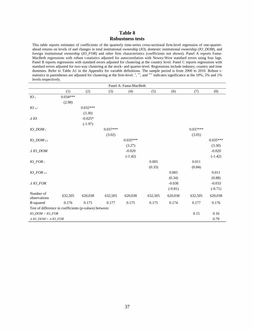
To further check the robustness of our results we complete our analysis with three additional

tests. First, we run Fama-MacBeth (1973) regressions and find no statistically significant

difference between the return forecasting power of domestic and foreign institutions (Table 8,

Panel A). Next, we perform the same regression but clustering standard errors at the country

level (Table 8, Panel B). Again, we cannot find a statistically significant difference between local

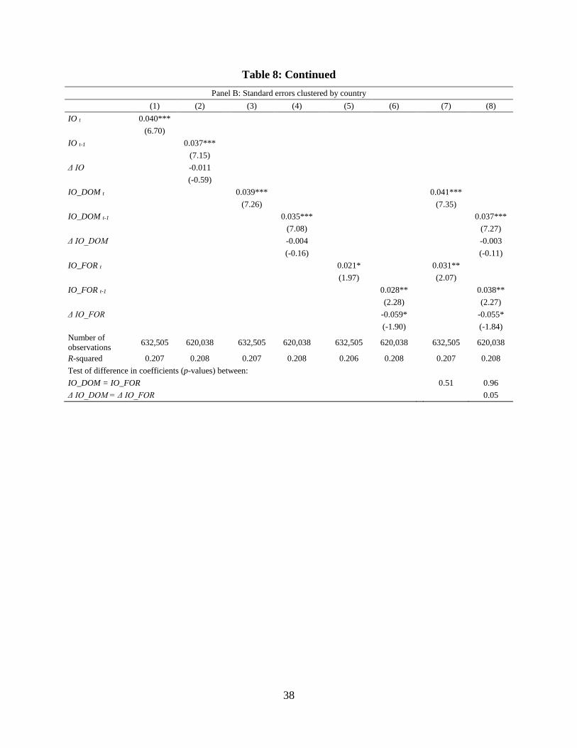
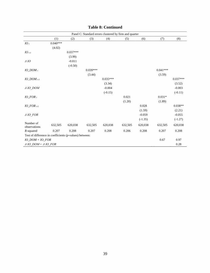
and foreign investors. Finally, we perform a regression with standard errors adjusted to two

dimensions of clustering: by stock and by quarter (Table 8, Panel C). We also cannot reject the

equality of coefficients between domestic and foreign institutional ownership.

In all three panels we find evidence of a price pressure effect, but no evidence for a smart

institutions effect. If anything, we find weak evidence that foreign institutions are at a slight

information disadvantage when standard errors are clustered at the country level (column (8) in

Panel B). To sum up, our additional tests show that our benchmark results are robust to different

forms of cross-sectional and temporal dependence.

6 Results on portfolio performance with these alternative classifications are available in the Internet Appendix.

22

6. Conclusion

We contribute to the literature by comparing the performance of domestic versus foreign

institutional holdings using a worldwide sample of stocks during the 2000-2010 period. We find

that, on average, domestic institutional investors perform as well as foreign institutional

investors. Both domestic and foreign institutional holdings are positively associated with future

returns, but this relation seems to come, on average, from a price-pressure effect, rather than

from superior information. The results are consistent with the notion that both capital markets

and asset management markets are efficient.

However, these averages mask conditional differences between local and foreign institutions.

Our results suggest that individual investors may benefit from allocating their wealth through

local money management companies when investing in countries where information asymmetry

is high. In these more difficult settings, only domestic institutional investors seem to trade with

an information advantage.

23

References

Albuquerque, R., G. Bauer, and M. Schneider, 2009, Global private information in international

equity markets, Journal of Financial Economics 94, 18-46.

Bae, K.-H., R. Stulz, and H. Tan, 2008, Do local analysts know more? A cross-country study of

the performance of local analysts and foreign analysts, Journal of Financial Economics 88,

581-606.

Baik, B., J.-K. Kang, and J.-M. Kim, 2010, Local institutional investors, information

asymmetries, and equity returns, Journal of Financial Economics 97, 81-106.

Bailey, W., C. Mao, and K. Sirodom, 2007, Investment restrictions and the cross-border flow of

information: Some empirical evidence, Journal of International Money and Finance 26, 1-

25.

Barberis, N., and A. Shleifer, 2003, Style investing, Journal of Financial Economics 68, 161-

199.

Brown, N., K. Wei, and R. Wermers, 2014, Analyst recommendations, mutual fund herding, and

overreaction in stock prices, Management Science 60, 1-20.

Carhart, M., 1997, On persistence in mutual fund performance, Journal of Finance 52, 57-82.

Chan, K., V. Covrig, and L. Ng, 2005, What determines the domestic bias and foreign bias?

Evidence from mutual fund equity allocations worldwide, Journal of Finance 60, 1495-

1534.

Choe, H., B.-C. Kho, and R. Stulz, 2005, Do domestic investors have an edge? The trading

experience of foreign investors in Korea, Review of Financial Studies 18, 795-829.

24

Chuprinin, O., M. Massa, and D. Schumacher, 2015, Outsourcing in the international mutual

fund industry: An equilibrium view, Journal of Finance 70, 2275-2308.

Cohen, R., P. Gompers, and T. Vuolteenaho, 2002, Who underreacts to cash-flow news?

Evidence from trading between individuals and institutions, Journal of Financial

Economics 66, 409-462.

Cole, H., G. Mailath, and A. Postlewaite, 2001, Investment and concern with relative position,

Review of Economic Design 6, 241-261.

Coval, J., and T. Moskowitz, 2001, The geography of investment: Informed trading and asset

prices, Journal of Political Economy 109, 811-841.

DeLong, J. B., A. Shleifer, L. Summers, and R. Waldmann, 1990, Noise trader risk in financial

markets, Journal of Political Economy 98, 703-738.

DeMarzo, P., R. Kaniel, and I. Kremer, 2004, Diversification as a public good: Community

effects in portfolio choice, Journal of Finance 59, 1677-1715.

Dvorak, T., 2005, Do domestic investors have an informational advantage? Evidence from

Indonesia, Journal of Finance 60, 817-840.

Fama, E., and J. MacBeth, 1973, Risk, return and equilibrium: Empirical tests, Journal of

Political Economy 81, 607-636.

Ferreira, M., and P. Matos, 2008, The colors of investors' money: The role of institutional

investors around the world, Journal of Financial Economics 88, 499-533.

Frankel, J., and K. Froot. 1987, Using survey data to test standard propositions regarding

exchange rate expectations, American Economic Review 77, 133-153.

25

French, K., and J. Poterba, 1991, Investor diversification and international equity markets,

American Economic Review 53, 222-226.

Froot, K., and T. Ramadorai, 2008, Institutional portfolio flows and international investments,

Review of Financial Studies 21, 937-971.

Froot, K., P. O’Connell, and M. Seasholes, 2001, The portfolio flows of international investors,

Journal of Financial Economics 59, 151-193.

Gehrig, T., 1993, An information based explanation of the domestic bias in international equity

investment, The Scandinavian Journal of Economics 21, 97-109.

Gompers, P., and A. Metrick, 2001, Institutional investors and equity prices, Quarterly Journal

of Economics 116, 229-259.

Grinblatt, M., and M. Keloharju, 2000, The investment behavior and performance of various

investor types: A study of Finland’s unique data set, Journal of Financial Economics 55,

43-67.

Hau, H., 2001, Location matters: An examination of trading profits, Journal of Finance 56,

1959-1983.

Hong, H., and J. Stein, 2003. Differences of opinion, short-sales constraints and market crashes,

Review of Financial Studies 16, 487-525.

Huang, R., and C.-Y. Shiu, 2005, Overseas monitors in emerging financial markets: Evidence

from foreign ownership in Taiwan, Working paper, University of Notre Dame.

Jegadeesh, N., and S. Titman, 1993, Returns to buying winners and selling losers: Implications

for stock market efficiency, Journal of Finance 48, 65-91.

26

Jin, L., and S. Myers, 2006, R2 around the world: New theory and new tests, Journal of Financial

Economics 79, 257-292.

Kang, J.-K., and R. Stulz, 1997, Why is there a home bias? An analysis of foreign portfolio

equity ownership in Japan, Journal of Financial Economics 46, 3-28.

Karolyi, G. A., and R. Stulz, 2003, Are assets priced locally or globally? Handbook of the

Economics of Finance, Elsevier Science, Amsterdam, The Netherlands.

Khorana, A., H. Servaes, and P. Tufano, 2005, Explaining the size of the mutual fund industry

around the world, Journal of Financial Economics 78, 145-185.

La Porta, R., F. Lopez-de-Silanes, A. Shleifer, and R. Vishny, 1998, Law and finance, Journal of

Political Economy 106, 1113-1155.

Leuz, C., K. Lins, and F. Warnock, 2009, Do foreigners invest less in poorly governed firms?

Review of Financial Studies 22, 3245-3285.

Lewis, K., 1999, Trying to explain the home bias in equities and consumption, Journal of

Economic Literature 37, 571-608.

Malloy, C., 2005, The geography of equity analysis, Journal of Finance 60, 719-755.

Morck, R., B. Yeung, and W. Yu, 2000, The information content of stock markets: Why do

emerging markets have synchronous stock price movements? Journal of Financial

Economics 58, 215-260.

Schmidt, P., U. Von Arx, A. Schrimpf, A. Wagner, and A. Ziegler, 2015, On the construction of

common size, value and momentum factors in international stock markets: A guide with

applications, Working Paper, ETH Zurich.

27

Seasholes, M., and N. Zhu, 2010, Individual investors and local bias, Journal of Finance 65,

1987-2011.

Shukla, R., and G. van Inwegen, 1995, Do locals perform better than foreigners? An analysis of

U.K. and U.S. mutual fund managers, Journal of Economics and Business 47, 241-254.

Teo, M., 2009, The geography of hedge funds, Review of Financial Studies 22, 3531-3561.

Van Nieuwerburgh, S., and L. Veldkamp, 2009, Information immobility and the home bias

puzzle, Journal of Finance 64, 1187-1215.

Wermers, R., T. Yao, and J. Zhao, 2012, Forecasting stock returns through an efficient

aggregation of mutual fund holdings, Review of Financial Studies 25, 3490-3529.

Zhang, X., 2006, information uncertainty and stock returns, Journal of Finance 61, 105-136.

28

Table 1

Domestic and foreign institutional ownership

This table reports, for each country in the sample, the average across all firms of total institutional ownership (IO), domestic

institutional ownership (IO_DOM), and foreign institutional ownership (IO_FOR) as a fraction of market capitalization as of

December 2010.

Country IO IO_DOM IO_FOR Number of

firms

Australia 0.156 0.022 0.134 821

Austria 0.179 0.018 0.162 69

Belgium 0.160 0.013 0.147 96

Brazil 0.252 0.047 0.205 153

Canada 0.498 0.272 0.227 675

China 0.184 0.022 0.162 442

Denmark 0.260 0.055 0.205 98

Finland 0.297 0.086 0.211 97

France 0.221 0.052 0.170 453

Germany 0.234 0.048 0.186 389

Hong Kong 0.144 0.027 0.117 853

India 0.137 0.040 0.097 1,340

Ireland 0.394 0.007 0.387 45

Israel 0.329 0.009 0.320 92

Italy 0.155 0.013 0.142 219

Japan 0.137 0.041 0.097 1,747

Korea (South) 0.149 0.001 0.148 779

Luxembourg 0.278 0.002 0.276 21

Malaysia 0.080 0.008 0.072 569

Netherlands 0.334 0.034 0.299 98

Norway 0.233 0.101 0.132 120

Poland 0.212 0.134 0.079 135

Portugal 0.115 0.010 0.105 37

Singapore 0.134 0.023 0.110 415

South Africa 0.213 0.046 0.166 180

Spain 0.168 0.014 0.154 119

Sweden 0.363 0.234 0.129 185

Switzerland 0.282 0.048 0.235 207

Taiwan 0.176 0.017 0.159 596

Thailand 0.121 0.019 0.102 324

U.K. 0.299 0.121 0.178 1,067

U.S. 0.728 0.649 0.079 3,916

Total 0.398 0.269 0.129 16,357

29

Table 2

Summary statistics

This table reports mean, median, standard deviation, minimum, maximum, and number of observations for firm-level

variables. Refer to Table A1 in the Appendix for variable definitions. The sample period is from 2000 to 2010.

Mean Median Standard deviation Minimum Maximum Observations

RET 0.032 0.012 0.277 -0.667 1.333 632,505

IO 0.206 0.072 0.282 0.000 1.000 632,505

IO_DOM 0.170 0.026 0.274 0.000 1.000 632,505

IO_FOR 0.036 0.006 0.073 0.000 1.000 632,505

BM 0.868 0.647 0.785 0.029 4.733 632,505

SIZE (million $) 2,029 188.6 10,600 10.00 571,197 632,505

VOL 0.145 0.115 0.123 0.009 1.467 632,505

TURN 1.117 0.540 1.679 0.001 12.605 632,505

PRICE 2.719 2.547 2.658 -3.297 11.419 632,505

MSCI 0.121 0.000 0.326 0.000 1.000 632,505

MOM 0.225 0.072 0.804 -0.894 5.044 632,505

DY 0.020 0.009 0.031 0.000 0.179 632,505

ADR 0.068 0.000 0.252 0.000 1.000 632,505

ANALYSTS 1.043 0.693 0.995 0.000 4.007 632,505

FXSALES 0.183 0.000 0.287 0.000 0.975 632,505

CLOSE 0.394 0.379 0.251 0.001 0.980 632,505

30

Table 3

Portfolio tests

This table shows value-weighted returns on the portfolios of domestic and foreign institutional holdings. The average monthly

return in excess of the risk-free rate, the alpha from the market model, and the alpha from the four-factor (Carhart) model are

shown. The four factors, expressed in U.S. dollars, are country-specific, except for the last three rows (“all countries”) where

the factors are global. The sample period is from 2000 to 2010.

Country

Excess Return Alpha (Market model) Alpha (Carhart model)

Domestic

holdings

Foreign

holdings

Difference

t-statistic

Domestic

holdings

Foreign

holdings

Difference

t-statistic

Domestic

holdings

Foreign

holdings

Difference

t-statistic

Australia 1.27% 1.45% -1.04 0.09% 0.22% -0.71 -0.02% 0.11% -0.65

Austria 1.19% 0.71% 2.92 0.17% -0.36% 3.23 0.28% -0.19% 2.52

Belgium 0.47% 0.24% 1.54 -0.12% -0.38% 1.80 -0.08% -0.16% 0.60

Brazil 1.92% 1.84% 0.25 -0.22% -0.30% 0.26 -0.16% -0.07% -0.27

Canada 0.89% 0.58% 1.05 -0.10% -0.58% 1.64 -0.04% -0.20% 0.56

China 1.52% 0.87% 1.53 0.94% 0.37% 1.38 0.78% 0.43% 0.94

Denmark 0.60% 0.98% -1.78 -0.37% 0.10% -2.21 -0.39% -0.01% -1.88

Finland 0.90% 0.02% 1.66 0.63% -0.39% 2.43 -0.04% -0.03% -0.03

France 0.27% 0.27% 0.01 -0.06% -0.06% -0.06 -0.06% -0.07% 0.07

Germany 0.27% 0.22% 1.05 -0.03% -0.08% 0.99 0.01% -0.01% 0.43

Hong Kong 0.84% 0.67% 1.62 0.22% 0.06% 1.55 0.21% 0.07% 1.31

India 1.55% 1.31% 1.30 0.02% -0.12% 0.76 0.09% 0.16% -0.44

Ireland 0.00% -0.03% 0.11 -0.23% -0.25% 0.06 -0.09% -0.12% 0.09

Israel -0.51% -0.73% 0.23 -0.38% -0.63% 0.27 0.55% -0.34% 1.00

Italy 0.07% 0.13% -0.77 0.03% 0.09% -0.81 0.05% 0.05% -0.01

Japan -0.34% -0.35% 0.10 -0.06% -0.07% 0.20 0.11% 0.06% 0.75

Korea (South) 1.16% 0.92% 0.93 0.27% 0.10% 0.68 0.18% 0.26% -0.34

Luxembourg 0.68% 0.65% 0.06 0.08% -0.19% 0.51 0.08% -0.12% 0.36

Malaysia 1.33% 1.48% -1.21 -0.22% -0.04% -1.35 -0.21% -0.07% -1.09

Netherlands 0.26% 0.27% -0.09 -0.08% -0.06% -0.23 -0.04% 0.02% -0.55

Norway 1.15% 1.19% -0.26 -0.09% -0.09% 0.01 0.19% -0.01% 1.52

Poland 1.82% 1.78% 0.20 0.04% 0.02% 0.09 -0.06% 0.09% -0.84

Portugal 0.44% 0.65% -0.78 -0.02% 0.21% -0.84 0.04% 0.27% -0.86

Singapore 0.67% 0.42% 0.46 -0.15% -0.55% 0.73 -0.17% 0.28% -0.84

South Africa 1.67% 1.61% 0.14 -0.12% -0.12% 0.00 -0.10% -0.10% 0.00

Spain 0.59% 0.53% 0.59 0.07% -0.02% 0.80 0.04% 0.01% 0.27

Sweden 0.48% 0.25% 1.89 -0.04% -0.27% 1.90 0.00% -0.12% 0.92

Switzerland 0.49% 0.37% 1.25 -0.03% -0.14% 1.11 -0.06% -0.09% 0.32

Taiwan 2.31% 2.39% -0.35 -0.21% 0.12% -1.46 -0.19% 0.14% -1.39

Thailand 1.75% 1.81% -0.54 0.15% 0.13% 0.16 0.14% 0.30% -1.42

United Kingdom 0.21% 0.10% 1.08 -0.02% -0.12% 0.98 0.00% -0.15% 1.48

United States 0.04% -0.02% 1.60 0.03% -0.04% 1.61 -0.01% -0.02% 0.11

All countries:

Domestic - Foreign 0.09% 0.18% -0.59 -0.12% -0.05% -0.43 -0.06% 0.04% -0.64

Same - Different Region 0.11% 0.13% -0.13 -0.10% -0.09% -0.04 -0.04% -0.02% -0.13

Close - Distant Investors 0.10% 0.17% -0.46 -0.11% -0.06% -0.34 -0.05% 0.03% -0.49

31

Table 4

Regression of future returns on levels of and changes in total, domestic and foreign

institutional ownership

This table reports estimates of coefficients of the quarterly time-series cross-sectional firm-level regression of one-quarter-

ahead returns on levels of and changes in total institutional ownership (IO), domestic institutional ownership (IO_DOM), and

foreign institutional ownership (IO_FOR) and other firm characteristics. Regressions include industry, country and time

dummies. Refer to Table A1 in the Appendix for variable definitions. The sample period is from 2000 to 2010. Robust t-

statistics in parentheses are adjusted for clustering at the firm-level. *, **, and *** indicates significance at the 10%, 5% and 1%

levels respectively.

(1) (2) (3) (4) (5) (6) (7) (8)

IO t 0.040***

(18.22)

IO t-1 0.037***

(16.93)

Δ IO -0.011

(-1.10)

IO_DOM t 0.039*** 0.041***

(17.29) (17.71)

IO_DOM t-1 0.035*** 0.037***

(15.50) (16.05)

Δ IO_DOM -0.004 -0.003

(-0.34) (-0.24)

IO_FOR t 0.021*** 0.031***

(3.98) (5.86)

IO_FOR t-1 0.028*** 0.038***

(5.38) (7.08)

Δ IO_FOR -0.059** -0.055**

(-2.19) (-2.04)

BM 0.018*** 0.019*** 0.018*** 0.019*** 0.019*** 0.019*** 0.018*** 0.019***

(32.89) (33.25) (32.78) (33.24) (34.97) (35.28) (32.78) (33.21)

SIZE -0.003*** -0.002*** -0.002*** -0.002*** -0.001** -0.001*** -0.003*** -0.002***

(-6.86) (-6.64) (-6.58) (-6.30) (-2.37) (-2.66) (-6.90) (-6.62)

VOL -0.084*** -0.078*** -0.084*** -0.078*** -0.091*** -0.085*** -0.084*** -0.078***

(-18.07) (-16.87) (-18.01) (-16.83) (-19.70) (-18.36) (-18.01) (-16.87)

TURN -0.005*** -0.004*** -0.005*** -0.004*** -0.004*** -0.003*** -0.005*** -0.004***

(-16.44) (-15.01) (-16.47) (-14.94) (-13.99) (-12.53) (-16.48) (-14.94)

PRICE -0.010*** -0.009*** -0.010*** -0.009*** -0.009*** -0.009*** -0.010*** -0.009***

(-28.23) (-27.41) (-27.85) (-27.03) (-27.20) (-26.49) (-28.07) (-27.31)

MSCI 0.006*** 0.006*** 0.007*** 0.007*** 0.002* 0.003*** 0.006*** 0.006***

(5.36) (5.90) (6.26) (6.60) (1.87) (2.61) (5.62) (5.88)

MOM 0.007*** 0.010*** 0.007*** 0.010*** 0.007*** 0.010*** 0.007*** 0.010***

(12.00) (15.92) (12.07) (15.85) (11.88) (15.61) (12.02) (15.93)

DY 0.220*** 0.212*** 0.219*** 0.211*** 0.205*** 0.199*** 0.220*** 0.212***

(17.50) (16.88) (17.39) (16.76) (16.39) (15.90) (17.50) (16.87)

ADR -0.002 -0.001 0.0002 0.0005 -0.004*** -0.004*** -0.001 -0.001

(-1.42) (-1.01) (0.15) (0.36) (-3.16) (-2.96) (-0.98) (-1.00)

ANALYSTS 0.010*** 0.009*** 0.010*** 0.010*** 0.012*** 0.011*** 0.010*** 0.009***

(17.47) (16.27) (18.60) (17.46) (20.75) (19.16) (17.53) (16.18)

FXSALES 0.005*** 0.005*** 0.006*** 0.006*** 0.005*** 0.005*** 0.005*** 0.005***

(3.42) (3.43) (3.92) (3.89) (3.72) (3.61) (3.52) (3.42)

CLOSE 0.017*** 0.017*** 0.016*** 0.016*** 0.013*** 0.013*** 0.017*** 0.017***

(10.40) (10.24) (9.79) (9.62) (7.95) (8.14) (10.28) (10.21)

Number of observations 632,505 620,038 632,505 620,038 632,505 620,038 632,505 620,038

R-squared 0.207 0.208 0.207 0.208 0.206 0.208 0.207 0.208

Test of difference in coefficients (p-values) between:

IO_DOM = IO_FOR 0.09 0.87

Δ IO_DOM = Δ IO_FOR 0.07

32

Table 5

Performance of portfolios sorted according to changes in Domestic and Foreign

Institutional Ownership

This table presents the time-series average of quarterly (rett,t+3) and yearly (rett,t+12) value-weighted returns on portfolios sorted

according to changes in foreign and domestic institutional ownership (IO). In each quarter, stocks are ranked into deciles

according to changes in IO, from largest ownership decreases (D1) to largest increases (D10). The row “Low (D1)” shows the

average next quarter return (rett,t+3) on: the stocks included in the D1 portfolio from the previous quarter (column j=1); the stocks

included in the two D1 portfolios from the previous two quarters (j=2); …; the stocks included in the four D1 portfolios from the

previous four quarters (j=4). The last column in each panel shows yearly returns (rett,t+12) on the stocks included in the four D1

portfolios from the previous four quarters (j=4). High-Low is a zero-cost investment strategy, which takes a long position in the

portfolio of stocks experiencing the largest ownership increases and a short position in the portfolio of stocks experiencing the

largest ownership decreases. We report average excess returns and Carhart four-factor alphas for the High-Low spreads, together

with t-statistics in parentheses.

Domestic Foreign

rett,t+3 rett,t+3 rett,t+3 rett,t+3 rett,t+12 rett,t+3 rett,t+3 rett,t+3 rett,t+3 rett,t+12

j=1 j=2 j=3 j=4 j=4

j=1 j=2 j=3 j=4 j=4

Low (D1) 0.67% 0.67% 1.19% 1.64% 6.01%

1.32% 1.37% 1.56% 1.93% 7.73%

High (D10) 0.51% 1.03% 1.26% 1.55% 5.33%

0.97% 1.20% 1.45% 1.81% 6.31%

High-Low (Excess return) -0.17% 0.35% 0.07% -0.08% -0.68% -0.35% -0.17% -0.10% -0.12% -1.42%

t-statistic (-0.38) (1.01) (0.27) (-0.44) (-0.94) (-1.14) (-0.66) (-0.43) (-0.50) (-1.23)

High-Low (4-Factor alpha) -0.20% 0.45% 0.27% -0.03% -1.31%

-0.35% -0.08% 0.05% 0.02% -0.33%

t-statistic (-0.37) (1.11) (1.06) (-0.14) (-1.55)

(-1.08) (-0.29) (0.24) (0.09) (-0.30)

33

Table 6

Regression of future returns on levels of and changes in local and nonlocal institutional ownership:

Effect of information asymmetry

This table reports estimates of coefficients of the quarterly time-series cross-sectional firm-level regression of one-quarter-ahead returns on levels of and changes in domestic

institutional ownership (IO_DOM) and foreign institutional ownership (IO_FOR), and other firm characteristics (coefficients not shown). Refer to Table A1 in the Appendix for

variable definitions. For each characteristic indicated in the table, stocks are divided into two subsamples according to the level of opaqueness revealed by that characteristic.

We classify as low opaqueness: U.S. firms; English-speaking countries; countries with low R2; countries with an accounting transparency index above the median; countries

with a corruption index above the median; countries with an anti-director rights index equal to or above 4; quarters in which the bull market dummy equals one; periods in

which the stress dummy equals zero; stocks covered by at least one analyst; stocks with return volatility below the median; firms with a fraction of shares held by insiders below

the median; firms with ownership concentration below the median; firms with market capitalization above the median; firms with a book-to-market equity ratio above the

median; and stocks with an illiquidity measure below the median. The high opaqueness group is formed with the remaining observations. Regressions include industry, country

and time dummies. The sample period is from 2000 to 2010. Robust t-statistics in parentheses are adjusted for clustering at the firm-level. *, **, and *** indicates significance at

the 10%, 5% and 1% levels respectively.

Characteristics Opaqueness IO_DOM t - 1 IO_FOR t - 1 Δ IO_DOM Δ IO_FOR Nr. of

obs.

R-

squared

Test of difference in coefficients

(p-value)

IO Δ IO

Panel A: Country characteristics

U.S. Low (U.S.) 0.039*** (11.71) 0.097*** (4.17) -0.026** (-2.04) -0.194*** (-3.35) 193,130 0.186 0.01 0.00

High (other) 0.015** (2.39) 0.019*** (3.58) 0.096*** (4.55) -0.038 (-1.27) 426,908 0.235 0.56 0.00

ENGLISH Low (Eng.) 0.033*** (12.70) 0.055*** (6.31) -0.010 (-0.83) -0.060 (-1.42) 347,966 0.211 0.02 0.25

High (other) 0.018* (1.83) 0.017** (2.52) 0.041 (1.44) -0.046 (-1.34) 272,072 0.229 0.93 0.05

CORRUPTION Low 0.036*** (14.91) 0.049*** (7.60) -0.020* (-1.85) -0.044 (-1.41) 472,892 0.198 0.05 0.47

High 0.060** (2.18) 0.014 (1.37) 0.145* (1.91) -0.048 (-0.83) 131,991 0.281 0.13 0.04

ANTI-DIRECTOR

Low 0.033*** (13.56) 0.054*** (7.09) -0.008 (-0.74) -0.042 (-1.18) 470,666 0.200 0.01 0.37

High 0.034*** (3.09) 0.024*** (3.06) 0.086*** (2.83) -0.079** (-2.00) 149,372 0.260 0.61 0.00

DISCLOSURE Low 0.036*** (14.92) 0.048*** (6.81) -0.007 (-0.66) -0.071** (-2.05) 526,604 0.200 0.10 0.08

High 0.064*** (4.83) 0.037*** (4.14) 0.032 (0.86) -0.044 (-1.05) 78,279 0.326 0.09 0.17

R2 Low 0.031*** (11.88) 0.052*** (6.17) -0.027** (-2.35) -0.066 (-1.54) 317,810 0.212 0.01 0.37

High 0.001 (0.09) 0.012* (1.70) 0.112*** (3.23) -0.036 (-1.06) 302,228 0.226 0.42 0.00

34

Table 6: Continued

Characteristic Opaqueness IO_DOM t - 1 IO_FOR t - 1 Δ IO_DOM Δ IO_FOR Nr. of obs.

R-squared

Test of difference

in coefficients (p-value)

IO Δ IO

Panel B: Market conditions

BULL/BEAR Low (Bull) 0.027*** (10.21) 0.044*** (7.02) -0.027** (-2.19) -0.029 (-0.88) 442,342 0.178 0.01 0.96

High (Bear) 0.055*** (12.42) -0.013 (-1.17) 0.077*** (3.69) -0.140*** (-3.18) 177,696 0.187 0.00 0.00

STRESS Low 0.031*** (11.29) 0.045*** (6.97) -0.007 (-0.59) -0.015 (-0.49) 435,983 0.111 0.04 0.82

High 0.046*** (11.12) -0.002 (-0.21) 0.020 (0.99) -0.197*** (-4.75) 184,055 0.299 0.00 0.00

Panel C: Stock characteristics

ANALYSTS Low 0.021*** (7.27) 0.050*** (8.69) -0.026** (-2.11) -0.058** (-2.26) 403,036 0.243 0.00 0.26

High 0.063*** (10.42) 0.015 (0.89) 0.068*** (2.95) -0.019 (-0.25) 217,002 0.167 0.01 0.28

VOL Low 0.013*** (5.37) 0.034*** (5.67) 0.013 (1.10) -0.038 (-1.44) 310,062 0.214 0.00 0.08

High 0.053*** (14.64) 0.033*** (3.81) -0.008 (-0.54) -0.068* (-1.76) 309,976 0.233 0.02 0.15

ILLIQ Low 0.031*** (10.41) 0.046*** (7.02) -0.010 (-0.78) -0.022 (-0.75) 305,893 0.243 0.04 0.72

High 0.059*** (10.44) 0.020* (1.87) 0.047** (2.51) -0.081 (-1.64) 304,602 0.192 0.00 0.02

CLOSE Low 0.038*** (12.76) 0.062*** (9.04) -0.022 (-1.58) -0.067** (-2.01) 310,074 0.213 0.00 0.21

High 0.039*** (9.26) 0.020** (2.27) 0.037** (2.07) -0.036 (-0.87) 309,964 0.209 0.05 0.11

HERF Low -0.029 (-1.37) 0.054*** (3.29) -0.024 (-0.54) 0.024 (0.35) 262,600 0.216 0.00 0.56

High 0.005* (1.79) 0.024*** (3.33) -0.037*** (-3.28) -0.095*** (-3.36) 264,968 0.242 0.01 0.06

SIZE Low 0.020*** (6.41) 0.023*** (4.02) 0.015 (1.20) -0.008 (-0.33) 310,032 0.247 0.60 0.41

High 0.061*** (11.89) 0.050*** (3.14) -0.007 (-0.37) -0.101* (-1.90) 310,006 0.195 0.51 0.10

BM Low 0.018*** (4.88) 0.044*** (4.92) 0.0004 (0.02) -0.097* (-1.92) 310,024 0.205 0.01 0.07

High 0.048*** (16.40) 0.032*** (4.78) 0.007 (0.54) -0.012 (-0.44) 310,014 0.215 0.02 0.53

35

Table 7

Regression of future returns on levels of and changes in institutional ownership: Alternative classifications

This table reports estimates of coefficients of the quarterly time-series cross-sectional firm-level regression of one-quarter-ahead returns on levels of and changes in total

institutional ownership (IO), domestic institutional ownership (IO_DOM), and foreign institutional ownership (IO_FOR) and other firm characteristics (coefficients not shown).

Panel A reports the results for institutional ownership based on the geographical region (same/different) of the stock and the institution. Panel B reports the results for

institutional ownership based on the distance between the capital city where the firm and institution are domiciled using a threshold of 1,000 km. Regressions include industry,

country and time dummies. Refer to Table A1 in the Appendix for variable definitions. The sample period is from 2000 to 2010. Robust t-statistics in parentheses are adjusted

for clustering at the firm-level. *, **, and *** indicates significance at the 10%, 5% and 1% levels respectively.

Panel A: Same and different region

(1) (2) (3) (4) (5) (6)

IO_SAME t 0.039*** 0.039***

(17.44) (17.74)

IO_SAME t-1 0.035*** 0.036***

(15.85) (16.24)

Δ IO_SAME -0.008 -0.007

(-0.73) (-0.63)

IO_DIFF t 0.029*** 0.040***

(3.98) (5.34)

IO_DIFF t-1 0.038*** 0.047***

(5.10) (6.34)

Δ IO_DIFF -0.053 -0.049

(-1.36) (-1.27)

Number of observations 632,505 620,038 632,505 620,038 632,505 620,038

R-squared 0.207 0.208 0.206 0.208 0.207 0.208

Test of difference in coefficients (p-values) between:

IO_SAME = IO_DIFF 0.97 0.15

Δ IO_SAME = Δ IO_DIFF 0.29

36

Table 7: Continued

Panel B: Local and distant

(1) (2) (3) (4) (5) (6)

IO_LOCAL t 0.038*** 0.040***

(17.31) (17.76)

IO_ LOCAL t-1 0.035*** 0.036***

(15.68) (16.24)

Δ IO_ LOCAL -0.008 -0.007

(-0.80) (-0.69)

IO_DISTANT t 0.023*** 0.037***

(3.73) (5.80)

IO_ DISTANT t-1 0.031*** 0.043***

(4.88) (6.76)

Δ IO_ DISTANT -0.042 -0.037

(-1.28) (-1.12)

Number of observations 632,505 620,038 632,505 620,038 632,505 620,038

R-squared 0.207 0.208 0.206 0.208 0.207 0.208

Test of difference in coefficients (p-values) between:

IO_LOCAL = IO_DISTANT 0.68 0.29

Δ IO_LOCAL = Δ IO_DISTANT 0.39

37

Table 8

Robustness tests

This table reports estimates of coefficients of the quarterly time-series cross-sectional firm-level regression of one-quarter-

ahead returns on levels of and changes in total institutional ownership (IO), domestic institutional ownership (IO_DOM), and

foreign institutional ownership (IO_FOR) and other firm characteristics (coefficients not shown). Panel A reports Fama-

MacBeth regressions with robust t-statistics adjusted for autocorrelation with Newey-West standard errors using four lags.

Panel B reports regressions with standard errors adjusted for clustering at the country level. Panel C reports regressions with

standard errors adjusted for two-way clustering at the stock- and quarter-level. Regressions include industry, country and time

dummies. Refer to Table A1 in the Appendix for variable definitions. The sample period is from 2000 to 2010. Robust t-

statistics in parentheses are adjusted for clustering at the firm-level. *, **, and *** indicates significance at the 10%, 5% and 1%

levels respectively.

Panel A: Fama-MacBeth

(1) (2) (3) (4) (5) (6) (7) (8)

IO t 0.034***

(2.98)

IO t-1 0.032***

(3.30)

Δ IO -0.025*

(-1.97)

IO_DOM t 0.037*** 0.037***

(3.02) (3.05)

IO_DOM t-1 0.035*** 0.035***

(3.27) (3.30)

Δ IO_DOM -0.020 -0.020

(-1.42) (-1.42)

IO_FOR t 0.005 0.011

(0.33) (0.84)

IO_FOR t-1 0.005 0.011

(0.34) (0.88)

Δ IO_FOR -0.038 -0.033

(-0.81) (-0.71)

Number of

observations 632,505 620,038 632,505 620,038 632,505 620,038 632,505 620,038

R-squared 0.176 0.175 0.177 0.175 0.175 0.174 0.177 0.176

Test of difference in coefficients (p-values) between:

IO_DOM = IO_FOR 0.15 0.16

Δ IO_DOM = Δ IO_FOR 0.79

38

Table 8: Continued

Panel B: Standard errors clustered by country

(1) (2) (3) (4) (5) (6) (7) (8)

IO t 0.040***

(6.70)

IO t-1 0.037***

(7.15)

Δ IO -0.011

(-0.59)

IO_DOM t 0.039*** 0.041***

(7.26) (7.35)

IO_DOM t-1 0.035*** 0.037***

(7.08) (7.27)

Δ IO_DOM -0.004 -0.003

(-0.16) (-0.11)

IO_FOR t 0.021* 0.031**

(1.97) (2.07)

IO_FOR t-1 0.028** 0.038**

(2.28) (2.27)

Δ IO_FOR -0.059* -0.055*

(-1.90) (-1.84)

Number of

observations 632,505 620,038 632,505 620,038 632,505 620,038 632,505 620,038

R-squared 0.207 0.208 0.207 0.208 0.206 0.208 0.207 0.208

Test of difference in coefficients (p-values) between:

IO_DOM = IO_FOR 0.51 0.96

Δ IO_DOM = Δ IO_FOR 0.05

39

Table 8: Continued

Panel C: Standard errors clustered by firm and quarter

(1) (2) (3) (4) (5) (6) (7) (8)

IO t 0.040***

(4.02)

IO t-1 0.037***

(3.99)

Δ IO -0.011

(-0.50)

IO_DOM t 0.039*** 0.041***

(3.44) (3.59)

IO_DOM t-1 0.035*** 0.037***

(3.34) (3.52)

Δ IO_DOM -0.004 -0.003

(-0.15) (-0.11)

IO_FOR t 0.021 0.031*

(1.20) (1.89)

IO_FOR t-1 0.028 0.038**

(1.59) (2.21)

Δ IO_FOR -0.059 -0.055

(-1.35) (-1.27)

Number of

observations 632,505 620,038 632,505 620,038 632,505 620,038 632,505 620,038

R-squared 0.207 0.208 0.207 0.208 0.206 0.208 0.207 0.208

Test of difference in coefficients (p-values) between:

IO_DOM = IO_FOR 0.67 0.97

Δ IO_DOM = Δ IO_FOR 0.28

40

Figure 1

Domestic and foreign institutional ownership

This figure shows the average institutional ownership by foreign and domestic institutions by country at the end of 2010.

Domestic (foreign) institutional ownership is the sum of the holdings of all institutions domiciled in the same country (in a

different country) in which the stock is listed, as a fraction of its year-end market capitalization.

41

Appendix

Table A1: Variables definition

Variable Definition

RET Quarterly stock return in US$ (Datastream item RI ($)).

IO Institutional ownership by all institutions as a percentage of market capitalization.

IO_DOM Institutional ownership by domestic institutions as a percentage of market capitalization.

IO_FOR Institutional ownership by foreign institutions as a percentage of market capitalization.

IO_SAME_REG Institutional ownership by institutions sharing the same geographic region as a percentage of market capitalization.

IO_DIFF_REG Institutional ownership by institutions not sharing the same geographic region as a percentage of market capitalization.

IO_LOCAL Institutional ownership by local (< 1000 kms) institutions as a percentage of market capitalization.

IO_DISTANT Institutional ownership by distant (>= 1000 kms) institutions as a percentage of market capitalization.

BM Log of the book-to-market equity ratio (market value is WorldScope item 08001 and book value is WorldScope item 03501).

SIZE Log market capitalization in US$ (Datastream item MV).

VOL Annualized standard deviation of monthly stock returns (Datastream).

TURN Ratio of share volume (Datastream item UVO) by the shares outstanding (Datastream item NOSH).

PRICE Log of the stock price (WorldScope item 05001).

MSCI MSCI member dummy, which equals one if a firm is in the MSCI All-Country World Index.

MOM 12-month trailing stock return in US$ (Datastream).

DY Dividend yield (WorldScope item 04551 divided by WorldScope item 08001).

ADR ADR dummy, which equals one if a firm is cross-listed on a U.S. exchange.

ANALYSTS Number of analysts covering a firm as reported by IBES.

FXSALES International annual net sales as a proportion of net sales (WorldScope item 08731).

CLOSE Number of shares held by insiders as a proportion of the number of shares outstanding (WorldScope item 08021).

ILLIQ Illiquidity measure computed as the number of days with zero returns in local currency divided by the number of observations in each year.

HERF Concentration of institutions’ holdings using the Herfindahl-Hirschman index - the sum of squares of the proportions of the firm’s shares held by institutional

investors. Large values of this index signify that the ownership is concentrated within a few large institutional holders.

BULL/BEAR Market condition dummy, which equals one during bull markets, and zero during bear markets.

VIX CBOE market volatility index (VXO index).

STRESS Uncertainty dummy, which equals one in quarters during which the VIX index exceeded its 75th percentile, and zero otherwise.

ENGLISH English speaking dummy, which equals one in English-speaking countries (Australia, Canada, Hong Kong, India, Ireland, South Africa, United Kingdom,

United States), and zero otherwise.

R2 R2 measures the percent of the variation in each country stock returns explained by variations in the country and U.S. stock market returns (Morck, Yeung, and

Yu (2000)). Stock markets with lower R2 are more efficient.

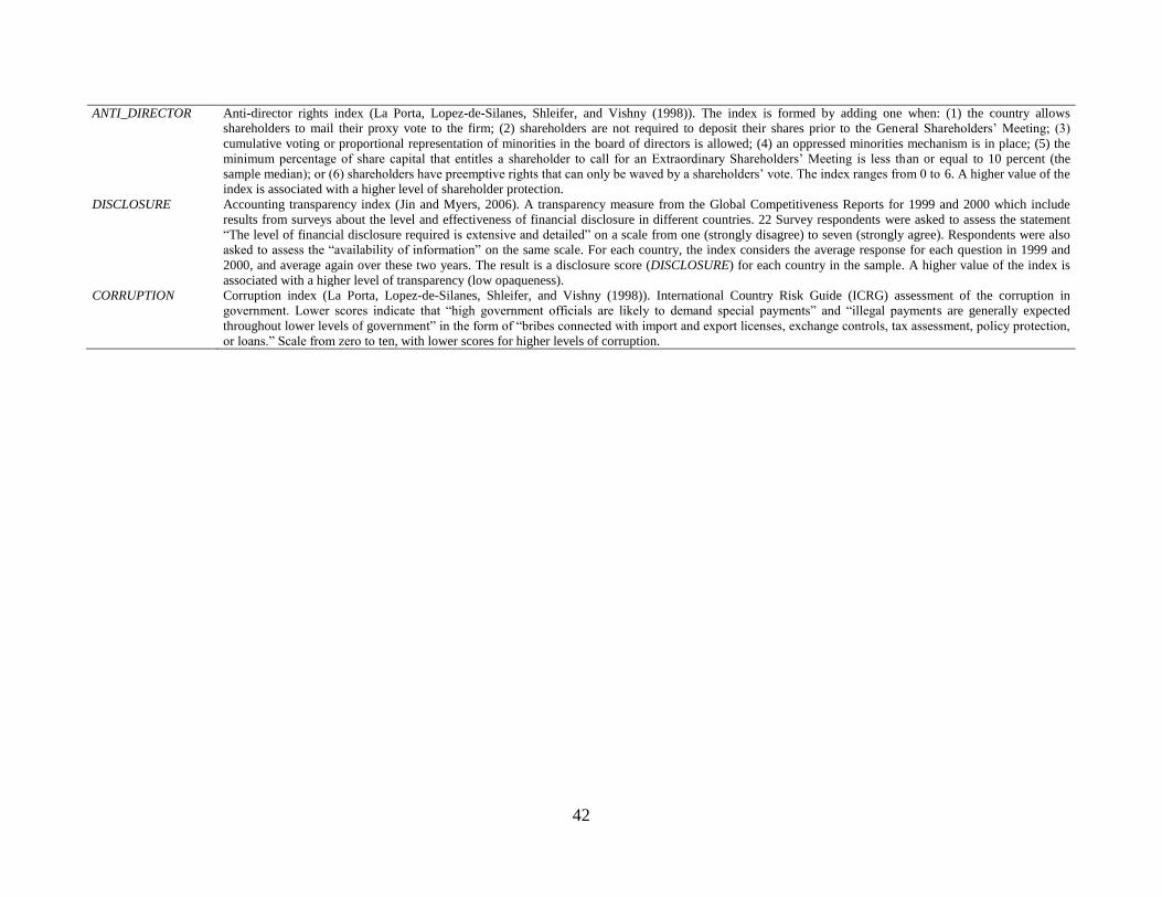
42

ANTI_DIRECTOR Anti-director rights index (La Porta, Lopez-de-Silanes, Shleifer, and Vishny (1998)). The index is formed by adding one when: (1) the country allows

shareholders to mail their proxy vote to the firm; (2) shareholders are not required to deposit their shares prior to the General Shareholders’ Meeting; (3)

cumulative voting or proportional representation of minorities in the board of directors is allowed; (4) an oppressed minorities mechanism is in place; (5) the

minimum percentage of share capital that entitles a shareholder to call for an Extraordinary Shareholders’ Meeting is less than or equal to 10 percent (the

sample median); or (6) shareholders have preemptive rights that can only be waved by a shareholders’ vote. The index ranges from 0 to 6. A higher value of the

index is associated with a higher level of shareholder protection.

DISCLOSURE Accounting transparency index (Jin and Myers, 2006). A transparency measure from the Global Competitiveness Reports for 1999 and 2000 which include

results from surveys about the level and effectiveness of financial disclosure in different countries. 22 Survey respondents were asked to assess the statement

“The level of financial disclosure required is extensive and detailed” on a scale from one (strongly disagree) to seven (strongly agree). Respondents were also

asked to assess the “availability of information” on the same scale. For each country, the index considers the average response for each question in 1999 and

2000, and average again over these two years. The result is a disclosure score (DISCLOSURE) for each country in the sample. A higher value of the index is

associated with a higher level of transparency (low opaqueness).

CORRUPTION Corruption index (La Porta, Lopez-de-Silanes, Shleifer, and Vishny (1998)). International Country Risk Guide (ICRG) assessment of the corruption in

government. Lower scores indicate that “high government officials are likely to demand special payments” and “illegal payments are generally expected

throughout lower levels of government” in the form of “bribes connected with import and export licenses, exchange controls, tax assessment, policy protection,

or loans.” Scale from zero to ten, with lower scores for higher levels of corruption.

Internet Appendix for

“Do Locals Know Better?

A Comparison of the Performance of Local and Foreign

Institutional Investors”

Miguel A. Ferreira

Nova School of Business and Economics

Pedro Matos

University of Virginia - Darden School of Business

João Pedro Pereira

Nova School of Business and Economics

Pedro Pires

Nova School of Business and Economics

This Version: May 2017

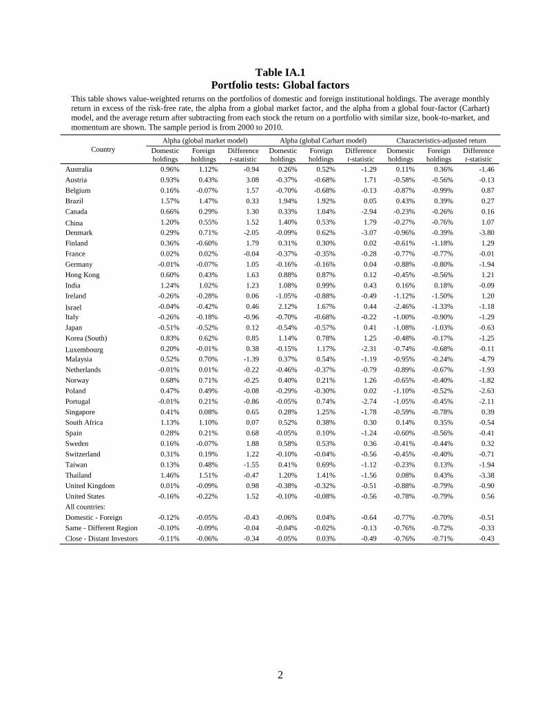
2

Table IA.1

Portfolio tests: Global factors

This table shows value-weighted returns on the portfolios of domestic and foreign institutional holdings. The average monthly

return in excess of the risk-free rate, the alpha from a global market factor, and the alpha from a global four-factor (Carhart)

model, and the average return after subtracting from each stock the return on a portfolio with similar size, book-to-market, and

momentum are shown. The sample period is from 2000 to 2010.

Country

Alpha (global market model) Alpha (global Carhart model) Characteristics-adjusted return

Domestic

holdings

Foreign

holdings

Difference

t-statistic

Domestic

holdings

Foreign

holdings

Difference

t-statistic

Domestic

holdings

Foreign

holdings

Difference

t-statistic

Australia 0.96% 1.12% -0.94 0.26% 0.52% -1.29 0.11% 0.36% -1.46

Austria 0.93% 0.43% 3.08 -0.37% -0.68% 1.71 -0.58% -0.56% -0.13

Belgium 0.16% -0.07% 1.57 -0.70% -0.68% -0.13 -0.87% -0.99% 0.87

Brazil 1.57% 1.47% 0.33 1.94% 1.92% 0.05 0.43% 0.39% 0.27

Canada 0.66% 0.29% 1.30 0.33% 1.04% -2.94 -0.23% -0.26% 0.16

China 1.20% 0.55% 1.52 1.40% 0.53% 1.79 -0.27% -0.76% 1.07

Denmark 0.29% 0.71% -2.05 -0.09% 0.62% -3.07 -0.96% -0.39% -3.80

Finland 0.36% -0.60% 1.79 0.31% 0.30% 0.02 -0.61% -1.18% 1.29

France 0.02% 0.02% -0.04 -0.37% -0.35% -0.28 -0.77% -0.77% -0.01

Germany -0.01% -0.07% 1.05 -0.16% -0.16% 0.04 -0.88% -0.80% -1.94

Hong Kong 0.60% 0.43% 1.63 0.88% 0.87% 0.12 -0.45% -0.56% 1.21

India 1.24% 1.02% 1.23 1.08% 0.99% 0.43 0.16% 0.18% -0.09

Ireland -0.26% -0.28% 0.06 -1.05% -0.88% -0.49 -1.12% -1.50% 1.20

Israel -0.04% -0.42% 0.46 2.12% 1.67% 0.44 -2.46% -1.33% -1.18

Italy -0.26% -0.18% -0.96 -0.70% -0.68% -0.22 -1.00% -0.90% -1.29

Japan -0.51% -0.52% 0.12 -0.54% -0.57% 0.41 -1.08% -1.03% -0.63

Korea (South) 0.83% 0.62% 0.85 1.14% 0.78% 1.25 -0.48% -0.17% -1.25

Luxembourg 0.20% -0.01% 0.38 -0.15% 1.17% -2.31 -0.74% -0.68% -0.11

Malaysia 0.52% 0.70% -1.39 0.37% 0.54% -1.19 -0.95% -0.24% -4.79

Netherlands -0.01% 0.01% -0.22 -0.46% -0.37% -0.79 -0.89% -0.67% -1.93

Norway 0.68% 0.71% -0.25 0.40% 0.21% 1.26 -0.65% -0.40% -1.82

Poland 0.47% 0.49% -0.08 -0.29% -0.30% 0.02 -1.10% -0.52% -2.63

Portugal -0.01% 0.21% -0.86 -0.05% 0.74% -2.74 -1.05% -0.45% -2.11

Singapore 0.41% 0.08% 0.65 0.28% 1.25% -1.78 -0.59% -0.78% 0.39

South Africa 1.13% 1.10% 0.07 0.52% 0.38% 0.30 0.14% 0.35% -0.54

Spain 0.28% 0.21% 0.68 -0.05% 0.10% -1.24 -0.60% -0.56% -0.41

Sweden 0.16% -0.07% 1.88 0.58% 0.53% 0.36 -0.41% -0.44% 0.32

Switzerland 0.31% 0.19% 1.22 -0.10% -0.04% -0.56 -0.45% -0.40% -0.71

Taiwan 0.13% 0.48% -1.55 0.41% 0.69% -1.12 -0.23% 0.13% -1.94

Thailand 1.46% 1.51% -0.47 1.20% 1.41% -1.56 0.08% 0.43% -3.38

United Kingdom 0.01% -0.09% 0.98 -0.38% -0.32% -0.51 -0.88% -0.79% -0.90

United States -0.16% -0.22% 1.52 -0.10% -0.08% -0.56 -0.78% -0.79% 0.56

All countries:

Domestic - Foreign -0.12% -0.05% -0.43 -0.06% 0.04% -0.64 -0.77% -0.70% -0.51

Same - Different Region -0.10% -0.09% -0.04 -0.04% -0.02% -0.13 -0.76% -0.72% -0.33

Close - Distant Investors -0.11% -0.06% -0.34 -0.05% 0.03% -0.49 -0.76% -0.71% -0.43

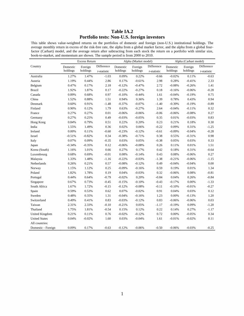
1

Table IA.2

Portfolio tests: Non-U.S. foreign investors

This table shows value-weighted returns on the portfolios of domestic and foreign (non-U.S.) institutional holdings. The

average monthly return in excess of the risk-free rate, the alpha from a global market factor, and the alpha from a global four-

factor (Carhart) model, and the average return after subtracting from each stock the return on a portfolio with similar size,

book-to-market, and momentum are shown. The sample period is from 2000 to 2010.

Country

Excess Return Alpha (Market model) Alpha (Carhart model)

Domestic holdings

Foreign holdings

Difference Domestic holdings

Foreign holdings

Difference Domestic holdings

Foreign holdings

Difference

t-statistic t-statistic t-statistic

Australia 1.27% 1.47% -1.03 0.09% 0.22% -0.66 -0.02% 0.11% -0.63

Austria 1.19% 0.44% 2.86 0.17% -0.61% 2.98 0.28% -0.41% 2.33

Belgium 0.47% 0.17% 2.18 -0.12% -0.47% 2.72 -0.08% -0.26% 1.41

Brazil 1.92% 1.87% 0.17 -0.22% -0.27% 0.18 -0.16% -0.06% -0.28

Canada 0.89% 0.68% 0.97 -0.10% -0.44% 1.61 -0.04% -0.19% 0.75

China 1.52% 0.88% 1.51 0.94% 0.36% 1.39 0.78% 0.43% 0.94

Denmark 0.60% 0.91% -1.48 -0.37% -0.07% -1.40 -0.39% -0.19% -0.89

Finland 0.90% 0.12% 1.79 0.63% -0.27% 2.64 -0.04% -0.11% 0.32

France 0.27% 0.27% 0.01 -0.06% -0.06% -0.06 -0.06% -0.08% 0.27

Germany 0.27% 0.25% 0.49 -0.03% -0.05% 0.35 0.01% -0.03% 0.83

Hong Kong 0.84% 0.79% 0.51 0.22% 0.20% 0.23 0.21% 0.18% 0.30

India 1.55% 1.49% 0.36 0.02% 0.06% -0.22 0.09% 0.31% -1.25

Ireland 0.00% 0.11% -0.60 -0.23% -0.12% -0.61 -0.09% -0.04% -0.28

Israel -0.51% -0.82% 0.34 -0.38% -0.71% 0.38 0.55% -0.31% 0.98

Italy 0.07% 0.09% -0.35 0.03% 0.05% -0.38 0.05% 0.03% 0.33

Japan -0.34% -0.35% 0.12 -0.06% -0.08% 0.26 0.11% 0.01% 1.51

Korea (South) 1.16% 1.01% 0.66 0.27% 0.17% 0.42 0.18% 0.31% -0.64

Luxembourg 0.68% 0.69% -0.01 0.08% -0.14% 0.43 0.08% -0.06% 0.27

Malaysia 1.33% 1.48% -1.16 -0.22% -0.03% -1.38 -0.21% -0.06% -1.15

Netherlands 0.26% 0.21% 0.57 -0.08% -0.12% 0.49 -0.04% -0.04% 0.00

Norway 1.15% 1.12% 0.25 -0.09% -0.16% 0.59 0.19% 0.01% 1.34

Poland 1.82% 1.78% 0.19 0.04% -0.03% 0.32 -0.06% 0.08% -0.81

Portugal 0.44% 0.64% -0.79 -0.02% 0.20% -0.84 0.04% 0.26% -0.84

Singapore 0.67% 0.73% -0.45 -0.15% -0.10% -0.43 -0.17% 0.00% -1.33

South Africa 1.67% 1.72% -0.15 -0.12% -0.08% -0.11 -0.10% -0.01% -0.27

Spain 0.59% 0.53% 0.62 0.07% -0.02% 0.91 0.04% 0.03% 0.12

Sweden 0.48% 0.35% 1.31 -0.04% -0.16% 1.23 0.00% -0.13% 1.20

Switzerland 0.49% 0.41% 0.83 -0.03% -0.12% 0.83 -0.06% -0.06% 0.03

Taiwan 2.31% 2.33% -0.10 -0.21% 0.05% -1.17 -0.19% 0.09% -1.20

Thailand 1.75% 1.81% -0.54 0.15% 0.12% 0.22 0.14% 0.27% -1.17

United Kingdom 0.21% 0.11% 0.76 -0.02% -0.12% 0.72 0.00% -0.05% 0.34

United States 0.04% -0.02% 1.60 0.03% -0.04% 1.61 -0.01% -0.02% 0.11

All countries:

Domestic - Foreign 0.09% 0.17% -0.63 -0.12% -0.06% -0.50 -0.06% -0.03% -0.25

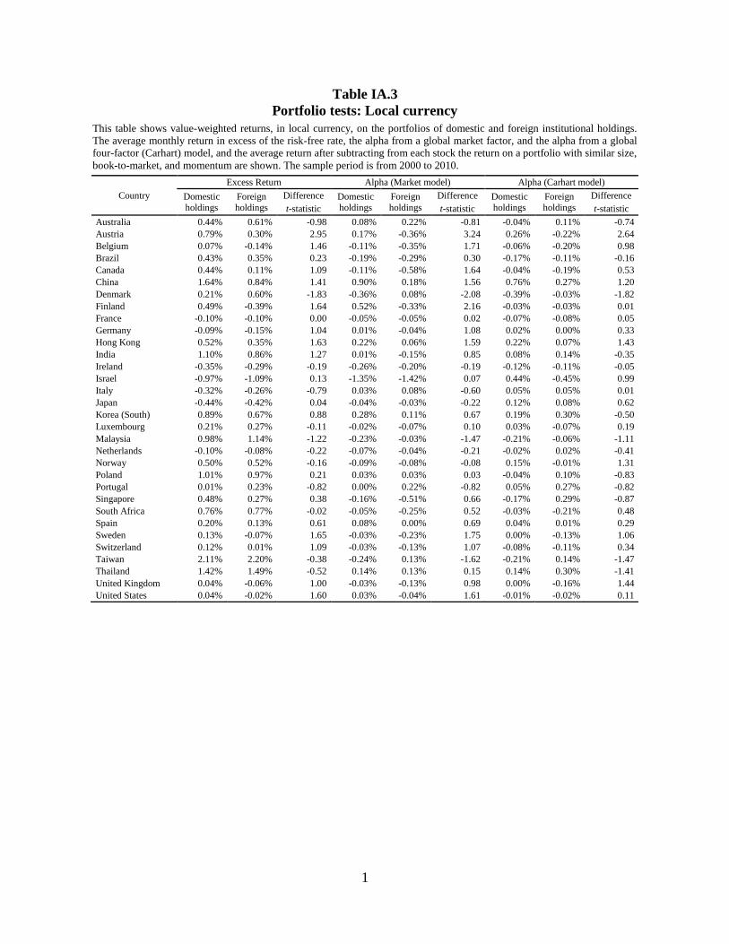
1

Table IA.3

Portfolio tests: Local currency

This table shows value-weighted returns, in local currency, on the portfolios of domestic and foreign institutional holdings.

The average monthly return in excess of the risk-free rate, the alpha from a global market factor, and the alpha from a global

four-factor (Carhart) model, and the average return after subtracting from each stock the return on a portfolio with similar size,

book-to-market, and momentum are shown. The sample period is from 2000 to 2010.

Country

Excess Return Alpha (Market model) Alpha (Carhart model)

Domestic

holdings

Foreign

holdings

Difference Domestic

holdings

Foreign

holdings

Difference Domestic

holdings

Foreign

holdings

Difference

t-statistic t-statistic t-statistic

Australia 0.44% 0.61% -0.98 0.08% 0.22% -0.81 -0.04% 0.11% -0.74

Austria 0.79% 0.30% 2.95 0.17% -0.36% 3.24 0.26% -0.22% 2.64

Belgium 0.07% -0.14% 1.46 -0.11% -0.35% 1.71 -0.06% -0.20% 0.98

Brazil 0.43% 0.35% 0.23 -0.19% -0.29% 0.30 -0.17% -0.11% -0.16

Canada 0.44% 0.11% 1.09 -0.11% -0.58% 1.64 -0.04% -0.19% 0.53

China 1.64% 0.84% 1.41 0.90% 0.18% 1.56 0.76% 0.27% 1.20

Denmark 0.21% 0.60% -1.83 -0.36% 0.08% -2.08 -0.39% -0.03% -1.82

Finland 0.49% -0.39% 1.64 0.52% -0.33% 2.16 -0.03% -0.03% 0.01

France -0.10% -0.10% 0.00 -0.05% -0.05% 0.02 -0.07% -0.08% 0.05

Germany -0.09% -0.15% 1.04 0.01% -0.04% 1.08 0.02% 0.00% 0.33

Hong Kong 0.52% 0.35% 1.63 0.22% 0.06% 1.59 0.22% 0.07% 1.43

India 1.10% 0.86% 1.27 0.01% -0.15% 0.85 0.08% 0.14% -0.35

Ireland -0.35% -0.29% -0.19 -0.26% -0.20% -0.19 -0.12% -0.11% -0.05

Israel -0.97% -1.09% 0.13 -1.35% -1.42% 0.07 0.44% -0.45% 0.99

Italy -0.32% -0.26% -0.79 0.03% 0.08% -0.60 0.05% 0.05% 0.01

Japan -0.44% -0.42% 0.04 -0.04% -0.03% -0.22 0.12% 0.08% 0.62

Korea (South) 0.89% 0.67% 0.88 0.28% 0.11% 0.67 0.19% 0.30% -0.50

Luxembourg 0.21% 0.27% -0.11 -0.02% -0.07% 0.10 0.03% -0.07% 0.19

Malaysia 0.98% 1.14% -1.22 -0.23% -0.03% -1.47 -0.21% -0.06% -1.11

Netherlands -0.10% -0.08% -0.22 -0.07% -0.04% -0.21 -0.02% 0.02% -0.41

Norway 0.50% 0.52% -0.16 -0.09% -0.08% -0.08 0.15% -0.01% 1.31

Poland 1.01% 0.97% 0.21 0.03% 0.03% 0.03 -0.04% 0.10% -0.83

Portugal 0.01% 0.23% -0.82 0.00% 0.22% -0.82 0.05% 0.27% -0.82

Singapore 0.48% 0.27% 0.38 -0.16% -0.51% 0.66 -0.17% 0.29% -0.87

South Africa 0.76% 0.77% -0.02 -0.05% -0.25% 0.52 -0.03% -0.21% 0.48

Spain 0.20% 0.13% 0.61 0.08% 0.00% 0.69 0.04% 0.01% 0.29

Sweden 0.13% -0.07% 1.65 -0.03% -0.23% 1.75 0.00% -0.13% 1.06

Switzerland 0.12% 0.01% 1.09 -0.03% -0.13% 1.07 -0.08% -0.11% 0.34

Taiwan 2.11% 2.20% -0.38 -0.24% 0.13% -1.62 -0.21% 0.14% -1.47

Thailand 1.42% 1.49% -0.52 0.14% 0.13% 0.15 0.14% 0.30% -1.41

United Kingdom 0.04% -0.06% 1.00 -0.03% -0.13% 0.98 0.00% -0.16% 1.44

United States 0.04% -0.02% 1.60 0.03% -0.04% 1.61 -0.01% -0.02% 0.11

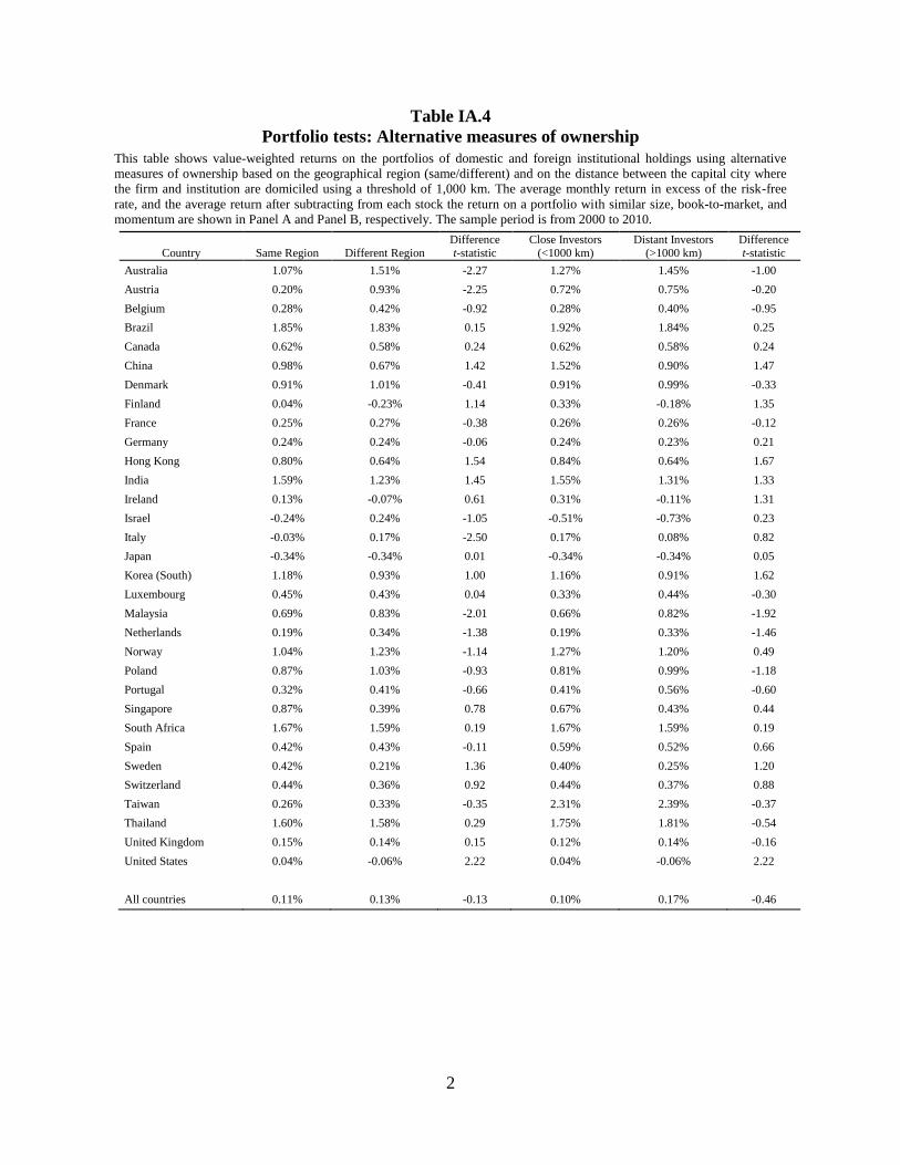
2

Table IA.4

Portfolio tests: Alternative measures of ownership

This table shows value-weighted returns on the portfolios of domestic and foreign institutional holdings using alternative

measures of ownership based on the geographical region (same/different) and on the distance between the capital city where

the firm and institution are domiciled using a threshold of 1,000 km. The average monthly return in excess of the risk-free

rate, and the average return after subtracting from each stock the return on a portfolio with similar size, book-to-market, and

momentum are shown in Panel A and Panel B, respectively. The sample period is from 2000 to 2010.

Country Same Region Different Region Difference t-statistic

Close Investors (<1000 km)

Distant Investors (>1000 km)

Difference t-statistic

Australia 1.07% 1.51% -2.27 1.27% 1.45% -1.00

Austria 0.20% 0.93% -2.25 0.72% 0.75% -0.20

Belgium 0.28% 0.42% -0.92 0.28% 0.40% -0.95

Brazil 1.85% 1.83% 0.15 1.92% 1.84% 0.25

Canada 0.62% 0.58% 0.24 0.62% 0.58% 0.24

China 0.98% 0.67% 1.42 1.52% 0.90% 1.47

Denmark 0.91% 1.01% -0.41 0.91% 0.99% -0.33

Finland 0.04% -0.23% 1.14 0.33% -0.18% 1.35

France 0.25% 0.27% -0.38 0.26% 0.26% -0.12

Germany 0.24% 0.24% -0.06 0.24% 0.23% 0.21

Hong Kong 0.80% 0.64% 1.54 0.84% 0.64% 1.67

India 1.59% 1.23% 1.45 1.55% 1.31% 1.33

Ireland 0.13% -0.07% 0.61 0.31% -0.11% 1.31

Israel -0.24% 0.24% -1.05 -0.51% -0.73% 0.23

Italy -0.03% 0.17% -2.50 0.17% 0.08% 0.82

Japan -0.34% -0.34% 0.01 -0.34% -0.34% 0.05

Korea (South) 1.18% 0.93% 1.00 1.16% 0.91% 1.62

Luxembourg 0.45% 0.43% 0.04 0.33% 0.44% -0.30

Malaysia 0.69% 0.83% -2.01 0.66% 0.82% -1.92

Netherlands 0.19% 0.34% -1.38 0.19% 0.33% -1.46

Norway 1.04% 1.23% -1.14 1.27% 1.20% 0.49

Poland 0.87% 1.03% -0.93 0.81% 0.99% -1.18

Portugal 0.32% 0.41% -0.66 0.41% 0.56% -0.60

Singapore 0.87% 0.39% 0.78 0.67% 0.43% 0.44

South Africa 1.67% 1.59% 0.19 1.67% 1.59% 0.19

Spain 0.42% 0.43% -0.11 0.59% 0.52% 0.66

Sweden 0.42% 0.21% 1.36 0.40% 0.25% 1.20

Switzerland 0.44% 0.36% 0.92 0.44% 0.37% 0.88

Taiwan 0.26% 0.33% -0.35 2.31% 2.39% -0.37

Thailand 1.60% 1.58% 0.29 1.75% 1.81% -0.54

United Kingdom 0.15% 0.14% 0.15 0.12% 0.14% -0.16

United States 0.04% -0.06% 2.22 0.04% -0.06% 2.22

All countries 0.11% 0.13% -0.13 0.10% 0.17% -0.46

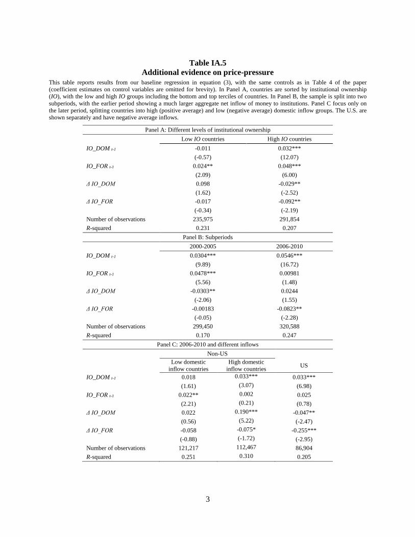
3

Table IA.5

Additional evidence on price-pressure

This table reports results from our baseline regression in equation (3), with the same controls as in Table 4 of the paper

(coefficient estimates on control variables are omitted for brevity). In Panel A, countries are sorted by institutional ownership

(IO), with the low and high IO groups including the bottom and top terciles of countries. In Panel B, the sample is split into two

subperiods, with the earlier period showing a much larger aggregate net inflow of money to institutions. Panel C focus only on

the later period, splitting countries into high (positive average) and low (negative average) domestic inflow groups. The U.S. are

shown separately and have negative average inflows.

Panel A: Different levels of institutional ownership

Low IO countries High IO countries

IO_DOM t-1 -0.011 0.032***

(-0.57) (12.07)

IO_FOR t-1 0.024** 0.048***

(2.09) (6.00)

Δ IO_DOM 0.098 -0.029**

(1.62) (-2.52)

Δ IO_FOR -0.017 -0.092**

(-0.34) (-2.19)

Number of observations 235,975 291,854

R-squared 0.231 0.207

Panel B: Subperiods

2000-2005 2006-2010

IO_DOM t-1 0.0304*** 0.0546***

(9.89) (16.72)

IO_FOR t-1 0.0478*** 0.00981

(5.56) (1.48)

Δ IO_DOM -0.0303** 0.0244

(-2.06) (1.55)

Δ IO_FOR -0.00183 -0.0823**

(-0.05) (-2.28)

Number of observations 299,450 320,588

R-squared 0.170 0.247

Panel C: 2006-2010 and different inflows

Non-US

Low domestic

inflow countries

High domestic

inflow countries US

IO_DOM t-1 0.018 0.033*** 0.033***

(1.61) (3.07) (6.98)

IO_FOR t-1 0.022** 0.002 0.025

(2.21) (0.21) (0.78)

Δ IO_DOM 0.022 0.190*** -0.047**

(0.56) (5.22) (-2.47)

Δ IO_FOR -0.058 -0.075* -0.255***

(-0.88) (-1.72) (-2.95)

Number of observations 121,217 112,467 86,904

R-squared 0.251 0.310 0.205