Disease and Development: The Effect of Life

Expectancy on Economic Growth∗

Daron AcemogluMIT

Simon JohnsonMIT

First Version: April 2004.Current Version: May 2006.

Abstract

What is the effect of increasing life expectancy on economic growth? To answer this ques-tion, we exploit the international epidemiological transition, the wave of international healthinnovations and improvements that began in the 1940s. We obtain estimates of mortality bydisease before the 1940s from the League of Nations and national public health sources. Usingthese data, we construct an instrument for changes in life expectancy, referred to as predictedmortality, which is based on the pre-intervention distribution of mortality from various diseasesaround the world and dates of global interventions. We document that predicted mortality hasa large and robust effect on changes in life expectancy starting in 1940, but no effect on changesin life expectancy before the interventions. The instrumented changes in life expectancy havea large effect on population; a 1% increase in life expectancy leads to an increase in populationof about 1.5%. Life expectancy has a much smaller effect on total GDP both initially andover a 40-year horizon, however. Consequently, there is no evidence that the large exogenousincrease in life expectancy led to a significant increase in per capita economic growth. Theseresults confirm that global efforts to combat poor health conditions in less developed countriescan be highly effective, but also shed doubt on claims that unfavorable health conditions arethe root cause of the poverty of some nations.

Keywords: disease environment, economic development, economic growth, health, inter-national epidemiological transition, life expectancy, mortality.

JEL Numbers: I10, O40, J11.

∗We thank Josh Angrist, David Autor, Abhijit Banerjee, Tim Besley, Anne Case, Sebnem Kalemli-Ozcan,Torsten Persson, Arvind Subramanian, David Weil, Pierre Yared and especially Angus Deaton for helpfulsuggestions and discussion. We also thank seminar participants at Brookings, Brown, Chicago, Harvard-MITDevelopment Seminar, LSE, Maryland, Northwestern, the NBER Summer Institute, Princeton, the SeventhBREAD Conference on Development Economics, and the World Bank for comments and the staff of the NationalLibrary of Medicine and MIT’s Retrospective Collection for their patient assistance.

1 Introduction

Improving health around the world today is an important social objective, which has obvious

direct payoffs in terms of longer and better lives for millions.1 There is also a growing consensus

that improving health can have equally large indirect payoffs through accelerating economic

growth.2 For example, Gallup and Sachs (2001, p. 91) argue that wiping out malaria in sub-

Saharan Africa could increase that continent’s per capita growth rate by as much as 2.6% a

year, and a recent report by the World Health Organization (2001) states:

“in today’s world, poor health has particularly pernicious effects on economic develop-

ment in sub-Saharan Africa, South Asia, and pockets of high disease and intense poverty

elsewhere” (p. 24) and

“...extending the coverage of crucial health services... to the world’s poor could save millions

of lives each year, reduce poverty, spur economic development and promote global security”

(p. i).

The evidence supporting this recent consensus is not yet conclusive, however. Although

cross-country regression studies show a strong correlation between measures of health (for

example, life expectancy or infant mortality) and both the level of economic development and

recent economic growth, these studies have not established a causal effect of health and disease

environments on economic growth. Since countries suffering from short life expectancy and

ill-health are also disadvantaged in other ways (and often this is the reason for their poor

health outcomes), such macro studies may be capturing the negative effects of these other,

often omitted, disadvantages. While a range of micro studies demonstrate the importance of

health for individual productivity, as discussed below, these studies do not resolve the question

of whether health differences are at the root of the large income differences we observe today

and whether improvements in health will increase economic growth substantially.

This paper investigates the effect of life expectancy at birth–as a general measure of the

health of the population–on economic growth. We exploit the large improvements in life

expectancy, especially among the relatively poor nations, driven by international health inter-

ventions, more effective public health measures, and the introduction of new chemicals and

drugs starting in the 1940s.3 This episode, which we refer to as the international epidemio-

logical transition, led to an unprecedented improvement in life expectancy in a large number

1See Becker, Phillipson and Soares (2005) and Deaton (2003 and 2004) for recent analyses.2See, among others, Bloom and Sachs (1998), Gallup and Sachs (2001), World Health Organization (2001),

Alleyne and Cohen (2002), Bloom and Canning (2005), and Lorentzon, Wacziarg, and McMillan (2005).3There were some effective medical and public health innovations prior to 1940. But the positive effects from

these innovations were concentrated in richer countries.

1

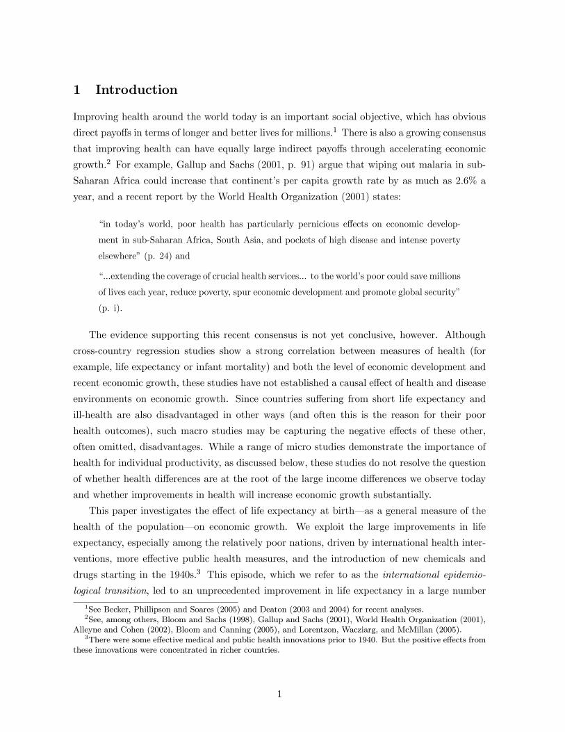
of countries.4 Figure 1 shows this by plotting life expectancy in countries that were initially

(circa 1940) poor, middle income, and rich. It illustrates that while in the 1930s life expectancy

was low in many poor and middle-income countries, this transition brought their levels of life

expectancy close to those prevailing in richer parts of the world.5 As a consequence of these

developments, health conditions in many parts of the less-developed world today, though still

in dire need of improvement, are significantly better than the corresponding health conditions

were in the West at the same stage of development.6

The international epidemiological transition provides us with an empirical strategy to iso-

late potentially-exogenous changes in health conditions. The effects of the international epi-

demiological transition on a country’s life expectancy were related to the extent to which its

population was initially (circa 1940) affected by various specific diseases, for example, tuber-

culosis, malaria, and pneumonia, and to the timing of the various health interventions.

The early data on mortality by disease are available from standard international sources,

though they have not been widely used in the economics literature. These data allow us to

create an instrument for changes in life expectancy based on the pre-intervention distribution

of mortality from various diseases around the world and the dates of global intervention (e.g.,

discovery and mass production of penicillin and streptomycin, or the discovery and widespread

use of DDT against mosquito vectors). The only source of variation in this instrument, which

we refer to as predicted mortality, comes from the interaction of baseline cross-country dis-

ease prevalence with global intervention dates for specific diseases. We document that there

were large declines in disease-specific mortality following these global interventions. More im-

4The term epidemiological transition was coined by demographers and refers to the process of falling mortalityrates after about 1850, associated with the switch from infectious to degenerative disease as the major cause ofdeath (Omran, 1971). Some authors prefer the term “health transition,” as this includes the changing natureof ill health more generally (e.g., Riley, 2001). Our focus is on the rapid decline in mortality (and improvementin health) in poorer countries after 1940, most of which was driven by the fast spread of new technologies andpractices around the world (hence the adjective “international”). The seminal works on this episode includeStolnitz (1955), Omran (1971), and Preston (1975a).

5This figure is for illustration purposes and should be interpreted with caution, since convergence is notgenerally invariant to nonlinear transformations. Our empirical strategy below does not exploit this convergencepattern; instead, it relies on potentially-exogenous changes in life expectancy.In these figures and throughout the paper, the initially rich countries are those with income per capita in 1940

above the level of Argentina (the richest Latin American country at that time, according to Maddison’s data, inour base sample). These are, in ascending order, Belgium, Netherlands, Sweden, Denmark, Canada, Germany,Australia, New Zealand, Switzerland, the United Kingdom and the United States. The initially poor countriesare those with income per capita below that of Portugal, which was the poorest European nation in our basesample. These are, in ascending order: China, Bangladesh, India, Pakistan, Myanmar, Thailand, El Salvador,Honduras, Indonesia, Brazil, Sri Lanka, Malaysia, Nicaragua, Korea, Ecuador, and the Philippines. Because ofdata quality issues, African nations are not included in our base sample, but they are used in robustness checksin Section 7. See Appendix Table A1 for a list of initially rich, middle-income and poor countries.

6For example, life expectancy at birth in India in 1999 was 60 compared to 40 in Britain in 1820, whenincome per capita was approximately the same level as in India today (Maddison, 2001, p. 30). From Maddison(2001, p. 264), income per capita in Britain in 1820 was $1707, while it stood at $1746 in India in 1998 (allfigures in 1990 international dollars).

2

portantly, we show that the predicted mortality instrument has a large and robust effect on

changes in life expectancy starting in 1940, but has no effect on changes in life expectancy

prior to this date (i.e., before the key interventions).

The instrumented changes in life expectancy have a fairly large effect on population; a

1% increase in life expectancy is related to an approximately 1.3-1.8% increase in population.

The magnitude of this estimate indicates that the decline in fertility rates was insufficient to

compensate for increased life expectancy, a result which we directly confirm by looking at the

relationship between life expectancy and total births.

On the other hand, we find no statistically significant effect on total GDP (though our

two standard error confidence intervals do include economically significant effects). More

importantly, relative growth rates for GDP per capita (and GDP per working age population)

show some decline in countries experiencing large increases in life expectancy. In fact, our

estimates exclude any positive effects of life expectancy on GDP per capita within a 40-year

horizon. This is consistent with the overall pattern in Figure 2, which, in contrast to Figure

1, shows no convergence in income per capita between initially poor, middle-income and rich

countries. Similarly, we find no evidence of an increase in human capital investments associated

with improvements in life expectancy.

The most natural interpretation of our results comes from neoclassical growth theory. The

first-order effect of increased life expectancy is to increase population, which initially reduces

capital-to-labor and land-to-labor ratios, thus depressing income per capita. This initial decline

is later compensated by higher output as more people enter the labor force. This compensa-

tion can be complete and may even exceed the initial level of income per capita if there are

significant productivity benefits from longer life expectancy. Yet, the compensation may also

be incomplete if the benefits from higher life expectancy are limited and if some factors of pro-

duction, for example land, are supplied inelastically. A smaller initial effect on GDP than the

longer-run effect is also consistent with the neoclassical growth model when the accumulation

of capital is slow.

The role of changes in capital-labor ratios in the above discussion also suggests that we

should expect less negative (or more positive) effects on income per capita in economies that

have higher investment rates. We investigate this by estimating models that allow for interac-

tions between life expectancy and initial GDP per capita or initial investment rates (for which

the data are less reliable), and find some support for this hypothesis.

Our findings do not imply that improved health has not been a great benefit to less-

developed nations during the postwar era. On the contrary, they suggest that global efforts

can significantly improve health conditions in less developed countries, and they may be able to

do so without large long-run costs in terms of income per capita. The accounting approach of

Becker, Philipson and Soares (2005), which incorporates information on longevity and health

3

as well as standards of living, would then suggest that these interventions have considerably

improved “overall welfare” in these countries. What these interventions have not done, and in

fact were not intended to do, is to increase output per capita in these countries.

Furthermore, our results, though suggestive, may not directly apply to the present date be-

cause of the different nature of diseases now prevalent in poor countries, in particular, because

of HIV/AIDS. Many of the diseases brought under greater control during the international

epidemiological transition were primarily killers of children.7 In contrast, arguably the most

serious health problem in the poorest parts of the world today, HIV/AIDS, affects those at

the peak of their labor productivity. Preventing HIV/AIDS could conceivably have different

effects from those we estimate here.

It is also important to note that the micro estimates have established beyond reasonable

doubt that improved health leads to better individual economic outcomes.8 Nevertheless,

these estimates do not directly answer the question of how important differences in disease en-

vironments and health conditions are in accounting for cross-country income disparities, and

are difficult to compare with our results, because they do not incorporate general equilibrium

effects (in addition, there still remains a great deal of uncertainty about the precise size of

the relevant effects). The most important general equilibrium effect arises because of dimin-

ishing returns to effective units of labor (for example, because land and/or physical capital

are supplied inelastically). In the presence of such diminishing returns, micro estimates will

exaggerate the aggregate productivity benefits from improved health, especially when health

improvements are accompanied by population increases. This may be an important concern

since existing estimates of production functions, theory and also our our results suggest that

there are indeed diminishing returns to labor.9

Our paper is most closely related to two recent contributions, Weil (2005) and Young

(2005). Weil calibrates the effects of health using a range of micro estimates, and finds that

7The exception is tuberculosis. The age profile of deaths from tuberculosis pre-1940 was closer to that ofAIDS today–with a heavy burden on young adults. The greatest impact of the remaining diseases were onchildren, but not necessarily on infants (e.g., endemic malaria typically has highest fatality rates for childrenbetween ages 1 and 5). Our analysis of the (somewhat less reliable) data on infant mortality shows no evidenceof a differential effect of the international epidemiological transition on infant mortality or survival rates (theseresults are not reported to save space).

8See Strauss and Thomas (1998) for an excellent survey of the research until the late 1990s. For some of themore recent research, see Behrman and Rosenzweig (2004), Bleakley (2002, 2004), Miguel and Kremer (2004),and Schultz (2002).

9Another general equilibrium effect arises when healthier individuals have higher earnings partly becausethey are successful in competing against less healthy individuals in the labor market (for example, for scarcehigh-paying jobs); when such competition effects are present, all individuals becoming healthier would havesmaller effects than those implied by the micro estimates. See Persico, Postlewaite and Silverman (2004) forevidence suggesting that the major effect of height on economic outcomes may be through a “competitiveadvantage” in adolescence.

4

these effects could be quite important in the aggregate (see also Bloom and Canning, 2005).10

The major difference between Weil’s approach and ours is that the conceptual exercise in

his paper is concerned with the effects of improved health holding population constant. In

contrast, our estimates look at the general equilibrium effects of improved health from the

most important health transition of the 20th century, which takes the form of both improved

health and increased life expectancy (and thus population). Young evaluates the effect of the

recent HIV/AIDS epidemic in Africa. Using micro estimates and calibration of the neoclassical

growth model, he shows that the decline in population resulting from HIV/AIDS may increase

income per capita despite significant disruptions and human suffering caused by the disease.11

In addition, our work is related to the literature on the demographic transition both in the

West and in the rest of the world, including the seminal contribution of McKeown (1976) and

studies by Arriaga and Davis (1969), Preston (1975a, 1980), Caldwell (1986), Kelley (1988),

Fogel (1986, 2004), and Deaton (2003, 2004). More recent work by Cutler and Miller (2005)

finds that the introduction of clean water accounts for about half of the decline in US mortality

in the early 20th century (see also Cutler and Miller, 2006).

The rest of the paper is organized as follows. In the next section, we present a simple

model to illustrate the factors that determine the effect of increased life expectancy on economic

growth. Section 3 describes the health interventions and the data on disease mortality rates and

life expectancy that we constructed from a variety of primary sources. Section 4 presents our

estimating framework and the ordinary least square (OLS) relationship between life expectancy

and a range of outcomes. Section 5 discusses the construction of our instrument and shows

the first-stage relationships, robustness checks, falsification exercises, and other supporting

evidence. Section 6 presents the main results. Section 7 presents a number of robustness checks

and additional results, and Section 8 concludes. Appendices A and B provide information on

data sources, data construction and the diseases used in this study. Appendix C, which provides

further details and some additional results, is available upon request.

2 Motivating Theory

To frame the empirical analysis, we first derive the medium-run and long-run implications of

increased life expectancy in the closed-economy neoclassical (Solow) growth model. All labor

and land are supplied inelastically. We represent all of health in terms of life expectancy.12

10Weil’s baseline estimate uses the return to the age of menarche from Knaul’s (2000) work on Mexico as ageneral indicator of “overall return to health”. Using Behrman and Rosenzweig’s (2004) estimates from returnsto birthweight differences in monozygotic twins, he finds smaller effects.11For more pessimistic views on the economic consequences of HIV/AIDS, see Arndt and Lewis (2000), Bell,

Devarajan, and Gersbach (2003) and Kalemli-Ozcan (2006).12Life expectancy here and throughout the paper is interpreted as a proxy (index) for the overall health of

the population. In practice, the decline in mortality from infectious disease and the corresponding increase

5

Economy i has the constant returns to scale aggregate production function

Yit = (AitHit)αKβ

itL1−α−βit , (1)

where α + β ≤ 1, Kit denotes capital, Lit denotes the supply of land, and Hit is the effective

units of labor given by

Hit = hitNit,

where Nit is total population (and hence employment), while hit is human capital per person.

Without loss of any generality, we normalize Lit = Li = 1 for all i and t. Let us also first as-

sume that Ait = Ai for all i and t. Capital depreciates at the rate δ and the savings/investment

rate of country i is constant and equal to si, which implies:

Kit+1 = siYit + (1− δ)Kit.

Suppose that there exists t < ∞ such that for all t ≥ t, human capital per person and

population are constant, i.e.,

hit = hi and Nit = Ni for all t ≥ t.

This implies that there exists a steady state, with Kit = Ki, satisfying

Ki =siδYi.

Substituting into (1) and taking logs we obtain a simple relationship between income per

capita, the savings rate, human capital, technology, and population:

yi ≡ log

µYiNi

¶(2)

=α

1− βlogAi +

α

1− βlog hi +

β

1− βlog si −

β

1− βlog δ − 1− α− β

1− βlogNi.

This equation shows that income per capita is affected positively by technology, Ai, human

capital, hi, and the investment rate, si, and negatively by population, Ni.

For industrialized economies where land plays a small role in production (because only a

small fraction of output is produced in agriculture), we can reasonably presume 1−α− β ' 0

in life expectancy resulting from the international epidemiological transition have been closely associated withincreased overall health and reduced morbidity (in particular, fewer incidences of illness from infectious disease,including less incapacity from tuberculosis, malaria, pneumonia, and lower incidence of illness in childhood).For example, before 1958 there were 817,000 cases of malaria in Venezuela, but after DDT spraying and othereradication efforts, there were only 800 cases. In Taiwan, there were about 1 million cases of malaria in 1954;a similar anti-malaria campaign was so effective that by 1969 there were only 9 cases. Most of these cases ofmalaria in both countries were associated with sickness and morbidity, not necessarily mortality (Lancaster,1990, Chapter 15). See also Riley (1993 and 2001) on the relationship between mortality and health in the19th-century Britain.

6

and population drops out of equation (2). Nevertheless, for many less-developed countries,

where agriculture is still important, we should expect 1−α−β > 0 and the direct effect of an

increase in population may be to reduce income per capita even in the steady state (i.e., even

once the capital stock has adjusted to the increase in population).13

Greater life expectancy will first lead to greater population (both directly and also poten-

tially indirectly by increasing total births), so we posit:

Nit = NiXλit, (3)

where Xit is life expectancy in country i at time t. Better health and longer life spans may

also increase productivity through a variety of channels, including more rapid human capital

accumulation or direct positive effects on (total factor) productivity.14 To capture the bene-

ficial effects of these variables on productivity emphasized in the literature, let us assume the

following isoelastic relationships:

Ait = AiXγit and hit = hiX

ηit, (4)

where Ai and hi are some baseline differences across countries.

To focus on long run (steady-state) relationships, suppose that Xit = Xi (at least for t ≥ t

for some t <∞), so that there exists a steady state relationship:

yi =α

1− βlog Ai +

α

1− βlog hi +

β

1− βlog si −

β

1− βlog δ (5)

−1− α− β

1− βlog Ni +

1

1− β(α (γ + η)− (1− α− β)λ)xi

where xi ≡ logXi is log life expectancy and recall that yi ≡ log (Yi/Ni).

An increase in life expectancy therefore leads to a significant increase in long-run income

per capita when there are limited diminishing returns (i.e., 1 − α − β is small) and when

life expectancy creates a substantial externality on technology (high γ) and/or encourages

significant increases in human capital (high η). On the contrary, when γ and η are small and

1 − α − β is large, an increase in life expectancy can reduce income per capita even in the

steady state.

13See Galor and Weil (2000), Hansen and Prescott (2002), and Galor (2005) for models in which at differentstages of development the relationship between population and income may change because of a change inthe composition of output or technology. In these models, during an early Malthusian phase, land plays animportant role as a factor of production and there are strong diminishing returns to capital. Later in thedevelopment process, the role of land diminishes, allowing per capita income growth. Hansen and Prescott(2002), for example, assume a Cobb-Douglas production function during the Malthusian phase with a share ofland equal to 0.3.14On the potential effects of life expectancy and health on productivity, see Bloom and Sachs (1998). On their

effects on human capital accumulation, see, among others, Kalemli-Ozcan, Ryder, and Weil (2000), Kalemli-Ozcan (2002) or Soares (2005), which point out that when people live longer, they will have greater incentivesto invest in human capital.

7

Equation (5) applies to the “long run” once the capital stock has adjusted to the increase

in population. It is also interesting to look at what happens to output in the “medium run”

where the capital stock is constant (or before it has fully adjusted). This medium-run scenario

would be particularly relevant to countries that have low savings rates and can only attract

limited foreign capital. To illustrate this point, consider the extreme case where the capital

stock is fixed at some value Ki. Then:

YiNi= Kβ

i (Aihi)αN

−(1−α)i

or substituting for (4) and (3), we have:

yi ≡ β log Ki + α log Ai + α log hi + (6)

− (1− α) log Ni + (α (γ + η)− (1− α)λ)xi.

Comparing this equation to equation (5), we see that the medium-run effect of an increase in

life expectancy is more negative (or less positive). This is intuitive: the response to an increase

in Ni before the capital stock adjusts to its new steady-state level will be a reduction in the

capital-labor ratio, further reducing income per capita.

Our empirical strategy below is to estimate equations similar to (5) and (6), and compare

the estimates to the parameters in these equations.

It is also evident that how quickly an economy approaches the long-run equilibrium depends

on its savings and investment rate. Therefore, this framework also suggests that we should

investigate the impact of the interaction between life expectancy and the investment rate on

the evolution of income per capita.

3 Background and Data

3.1 International Epidemiological Transition

Early improvements in public health began in Western Europe, the United States and a few

other places from the mid-nineteenth century.15 Initially progress was through empirically

observing what worked, but soon came major breakthroughs connected with the germ theory

of disease. By 1900, tropical medicine had also made impressive progress, most notably with

Ronald Ross’s demonstration that mosquitoes transmitted malaria and with practical advances

against yellow fever in the Caribbean.

Nevertheless, through 1940 most of the progress in improving mortality was confined to

relatively rich countries, with some–but more limited–impact in Southern and Eastern Eu-

15Cutler, Deaton, Lleras-Murray (2006, pp. 11-12) also point out that new drugs, primarily antibiotics andsulphonamide drugs, had an important impact on US mortality between the 1930s and 1960.

8

rope. In most of the Americas, Africa, and Asia, there were even more limited improvements.16

In part, this was because there were few effective drugs against major killers, so most of the

measures were relatively expensive public works (e.g., to drain swamps). Colonial authorities

showed little enthusiasm for such expenditure.

The situation changed dramatically from around 1940 mainly because of four factors. First,

there was a wave of global drug innovations. Many of these products offered cures effective

against major killers in developing countries. The most important was the discovery and

subsequent mass production of penicillin, which provided an effective treatment against a

range of bacterial infections (National Academy of Sciences, 1970, Easterlin, 1999). Penicillin,

which was only used in small quantities even in the most developed countries through the mid-

1940s (Conybeare, 1948, p. 66), became widely available by the early 1950s (see, e.g., Valentine

and Shooter, 1954).17 Further antibiotic development quickly followed, most notably with the

discovery of streptomycin, which was effective against tuberculosis. Between 1940 and 1950,

the major bacterial killers became treatable and, in most cases, curable. Diseases that could

now be treated, for most people without serious side effects, included pneumonia, dysentery,

cholera, and venereal diseases. Antibiotics also reduced deaths indirectly caused by (and

attributed to) viruses, such as influenza, which often kill by weakening the immune system

and allowing secondary bacterial infections to develop. Also important during the same period

was the development of new vaccines, for example, against yellow fever.18

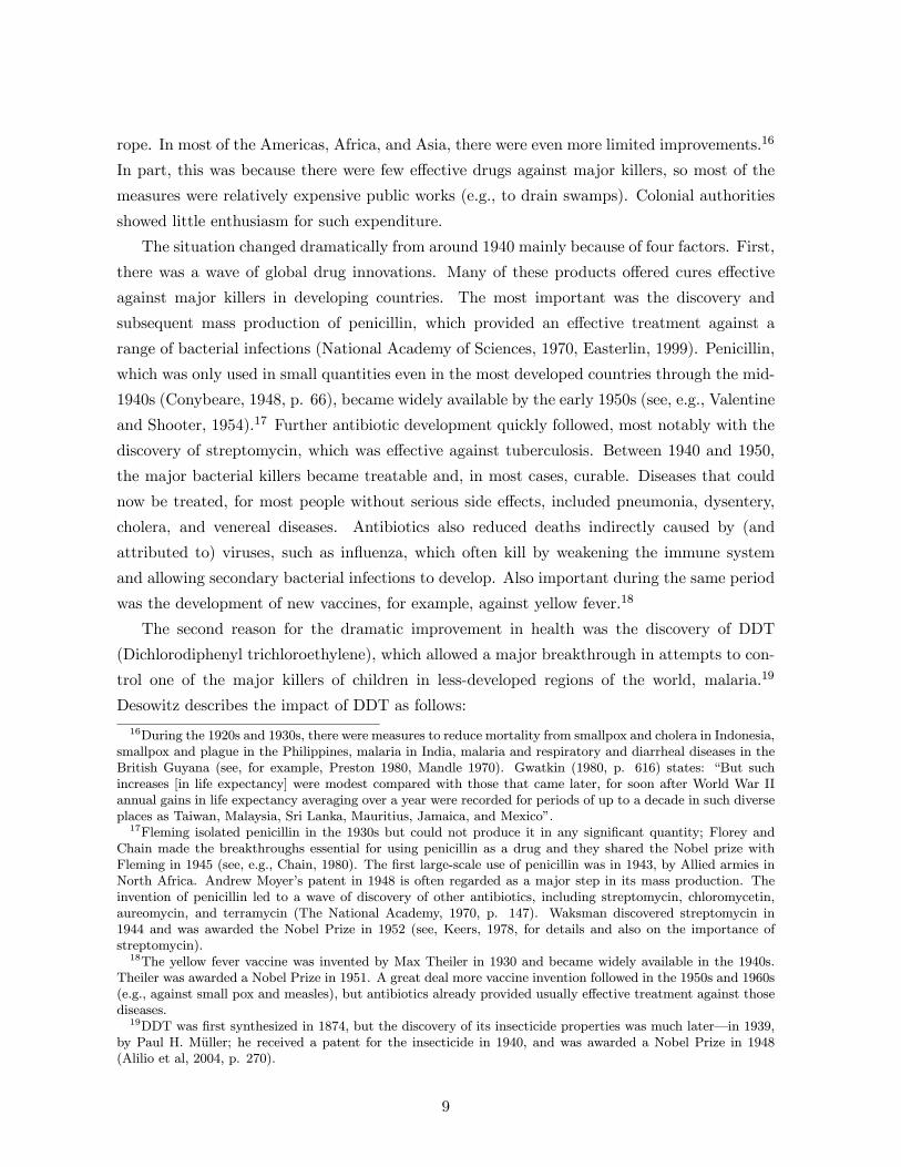
The second reason for the dramatic improvement in health was the discovery of DDT

(Dichlorodiphenyl trichloroethylene), which allowed a major breakthrough in attempts to con-

trol one of the major killers of children in less-developed regions of the world, malaria.19

Desowitz describes the impact of DDT as follows:

16During the 1920s and 1930s, there were measures to reduce mortality from smallpox and cholera in Indonesia,smallpox and plague in the Philippines, malaria in India, malaria and respiratory and diarrheal diseases in theBritish Guyana (see, for example, Preston 1980, Mandle 1970). Gwatkin (1980, p. 616) states: “But suchincreases [in life expectancy] were modest compared with those that came later, for soon after World War IIannual gains in life expectancy averaging over a year were recorded for periods of up to a decade in such diverseplaces as Taiwan, Malaysia, Sri Lanka, Mauritius, Jamaica, and Mexico”.17Fleming isolated penicillin in the 1930s but could not produce it in any significant quantity; Florey and

Chain made the breakthroughs essential for using penicillin as a drug and they shared the Nobel prize withFleming in 1945 (see, e.g., Chain, 1980). The first large-scale use of penicillin was in 1943, by Allied armies inNorth Africa. Andrew Moyer’s patent in 1948 is often regarded as a major step in its mass production. Theinvention of penicillin led to a wave of discovery of other antibiotics, including streptomycin, chloromycetin,aureomycin, and terramycin (The National Academy, 1970, p. 147). Waksman discovered streptomycin in1944 and was awarded the Nobel Prize in 1952 (see, Keers, 1978, for details and also on the importance ofstreptomycin).18The yellow fever vaccine was invented by Max Theiler in 1930 and became widely available in the 1940s.

Theiler was awarded a Nobel Prize in 1951. A great deal more vaccine invention followed in the 1950s and 1960s(e.g., against small pox and measles), but antibiotics already provided usually effective treatment against thosediseases.19DDT was first synthesized in 1874, but the discovery of its insecticide properties was much later–in 1939,

by Paul H. Muller; he received a patent for the insecticide in 1940, and was awarded a Nobel Prize in 1948(Alilio et al, 2004, p. 270).

9

“There was nothing quite like [DDT] before and has been nothing quite like it since. Here

was a chemical that could be sprayed on the walls of a house and for up to six months later

any insect that alighted or rested on that wall would die. It was virtually without toxicity

to humans. And, for the icing on the chemical cake, it was dirt-cheap to manufacture”

(1991, pp. 62-63).

Aggressive use of inexpensive DDT led to the rapid eradication of malaria in Taiwan, much of

the Caribbean, the Balkans, parts of northern Africa, northern Australia, large parts of South

Pacific, and all but eradicated malaria in Sri Lanka and India (see, e.g., Davis, 1956).

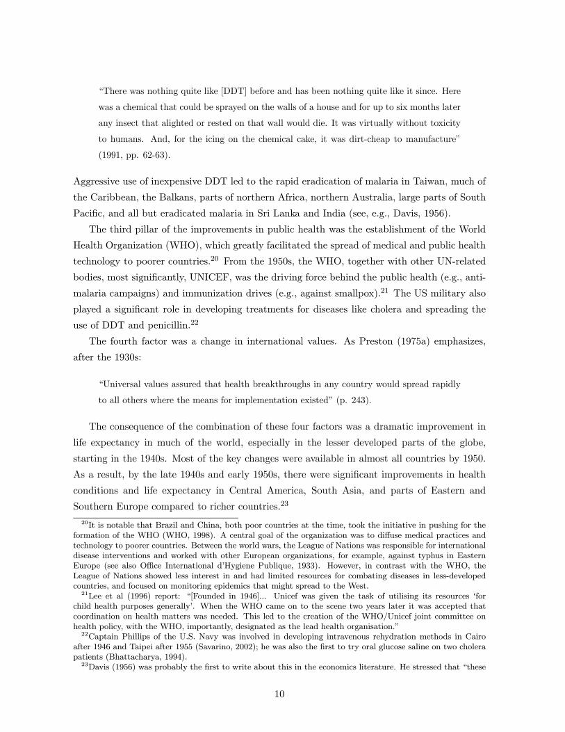
The third pillar of the improvements in public health was the establishment of the World

Health Organization (WHO), which greatly facilitated the spread of medical and public health

technology to poorer countries.20 From the 1950s, the WHO, together with other UN-related

bodies, most significantly, UNICEF, was the driving force behind the public health (e.g., anti-

malaria campaigns) and immunization drives (e.g., against smallpox).21 The US military also

played a significant role in developing treatments for diseases like cholera and spreading the

use of DDT and penicillin.22

The fourth factor was a change in international values. As Preston (1975a) emphasizes,

after the 1930s:

“Universal values assured that health breakthroughs in any country would spread rapidly

to all others where the means for implementation existed” (p. 243).

The consequence of the combination of these four factors was a dramatic improvement in

life expectancy in much of the world, especially in the lesser developed parts of the globe,

starting in the 1940s. Most of the key changes were available in almost all countries by 1950.

As a result, by the late 1940s and early 1950s, there were significant improvements in health

conditions and life expectancy in Central America, South Asia, and parts of Eastern and

Southern Europe compared to richer countries.23

20It is notable that Brazil and China, both poor countries at the time, took the initiative in pushing for theformation of the WHO (WHO, 1998). A central goal of the organization was to diffuse medical practices andtechnology to poorer countries. Between the world wars, the League of Nations was responsible for internationaldisease interventions and worked with other European organizations, for example, against typhus in EasternEurope (see also Office International d’Hygiene Publique, 1933). However, in contrast with the WHO, theLeague of Nations showed less interest in and had limited resources for combating diseases in less-developedcountries, and focused on monitoring epidemics that might spread to the West.21Lee et al (1996) report: “[Founded in 1946]... Unicef was given the task of utilising its resources ‘for

child health purposes generally’. When the WHO came on to the scene two years later it was accepted thatcoordination on health matters was needed. This led to the creation of the WHO/Unicef joint committee onhealth policy, with the WHO, importantly, designated as the lead health organisation.”22Captain Phillips of the U.S. Navy was involved in developing intravenous rehydration methods in Cairo

after 1946 and Taipei after 1955 (Savarino, 2002); he was also the first to try oral glucose saline on two cholerapatients (Bhattacharya, 1994).23Davis (1956) was probably the first to write about this in the economics literature. He stressed that “these

10

3.2 Coding Diseases

Central to our empirical strategy is to construct cross-country mortality rates for various

diseases before the 1940s. For this purpose, we have collected comparable data on 15 of the

most important infectious diseases across a wide range of countries. In all cases, the primary

data source is national health statistics, as collected and republished by the League of Nations

(until 1940) and the World Health Organization and the United Nations (after 1945). We have

tried several different ways of constructing these data, all of which produce similar results.

We confirm the validity of these numbers using the qualitative and quantitative evidence

in Lancaster (1990, especially, Chapter 48), the maps and discussion of Cliff, Haggett, and

Smallman-Raynor (2004) and the maps of disease incidence published by the American Geo-

graphical Society (1951a, b, c, and d) immediately after World War II. Appendix A provides

details on sources and construction. Further details are contained in Appendix C. Information

on the etiology and epidemiology of each disease is obtained from the comprehensive recent

surveys in Kiple (1993) and other sources (see Appendix B). To the extent possible, we have

also checked our data against those reported in Preston and Nelson (1974).

The other building block for our approach is global intervention dates for each specific

disease, that is, dates of significant events potentially reducing mortality around the world

from the disease in question. These events are described below (and in Appendix B) and the

relevant dates were obtained fromWHO Epidemiological Reports, as well as National Academy

of Sciences (1970), Preston (1975a), Kiple (1993), Easterlin (1999), and Hoff and Smith (2000).

The 15 diseases we focus on are tuberculosis, malaria, pneumonia, influenza, cholera, ty-

phoid, smallpox, whooping cough, measles, diphtheria, scarlet fever, yellow fever, plague, ty-

phus fever, and dysentery. The most important killers in this list are tuberculosis, malaria,

and pneumonia, which we discuss in this section. Information about the remaining diseases is

summarized in Appendix B.

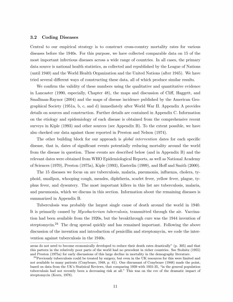
Tuberculosis was probably the largest single cause of death around the world in 1940.

It is primarily caused by Mycobacterium tuberculosis, transmitted through the air. Vaccina-

tion had been available from the 1920s, but the breakthrough cure was the 1944 invention of

streptomycin.24 The drug spread quickly and has remained important. Following the above

discussion of the invention and introduction of penicillin and streptomycin, we code the inter-

vention against tuberculosis in the 1940s.

areas do not need to become economically developed to reduce their death rates drastically” (p. 305) and thatthis pattern in the relatively poor parts of the world had no precedent in richer countries. See Stolnitz (1955)and Preston (1975a) for early discussions of this large decline in mortality in the demography literature.24Previously tuberculosis could be treated by surgery, but even in the UK resources for this were limited and

not available to many patients (Conybeare, 1948, p. 61). One discussant of Conybeare (1948) made the point,based on data from the UK’s Statisical Reviews, that comparing 1939 with 1931-35, “in the general populationtuberculosis had not recently been a decreasing risk at all.” This was on the eve of the dramatic impact ofstreptomycin (Keers, 1978).

11

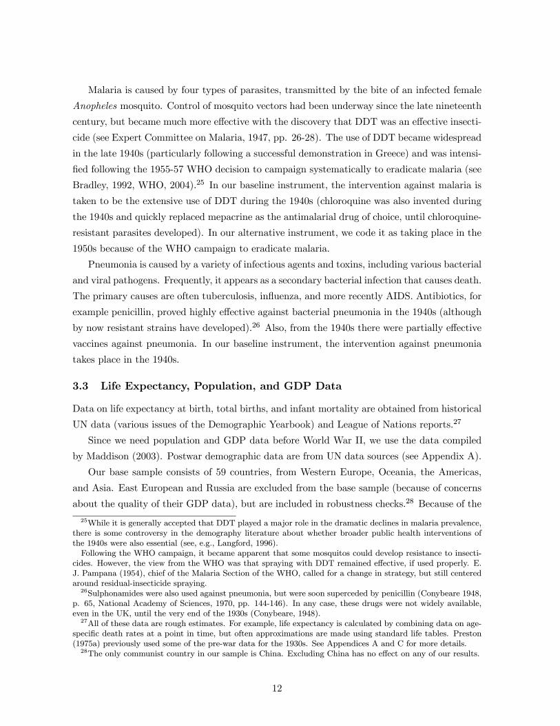
Malaria is caused by four types of parasites, transmitted by the bite of an infected female

Anopheles mosquito. Control of mosquito vectors had been underway since the late nineteenth

century, but became much more effective with the discovery that DDT was an effective insecti-

cide (see Expert Committee on Malaria, 1947, pp. 26-28). The use of DDT became widespread

in the late 1940s (particularly following a successful demonstration in Greece) and was intensi-

fied following the 1955-57 WHO decision to campaign systematically to eradicate malaria (see

Bradley, 1992, WHO, 2004).25 In our baseline instrument, the intervention against malaria is

taken to be the extensive use of DDT during the 1940s (chloroquine was also invented during

the 1940s and quickly replaced mepacrine as the antimalarial drug of choice, until chloroquine-

resistant parasites developed). In our alternative instrument, we code it as taking place in the

1950s because of the WHO campaign to eradicate malaria.

Pneumonia is caused by a variety of infectious agents and toxins, including various bacterial

and viral pathogens. Frequently, it appears as a secondary bacterial infection that causes death.

The primary causes are often tuberculosis, influenza, and more recently AIDS. Antibiotics, for

example penicillin, proved highly effective against bacterial pneumonia in the 1940s (although

by now resistant strains have developed).26 Also, from the 1940s there were partially effective

vaccines against pneumonia. In our baseline instrument, the intervention against pneumonia

takes place in the 1940s.

3.3 Life Expectancy, Population, and GDP Data

Data on life expectancy at birth, total births, and infant mortality are obtained from historical

UN data (various issues of the Demographic Yearbook) and League of Nations reports.27

Since we need population and GDP data before World War II, we use the data compiled

by Maddison (2003). Postwar demographic data are from UN data sources (see Appendix A).

Our base sample consists of 59 countries, from Western Europe, Oceania, the Americas,

and Asia. East European and Russia are excluded from the base sample (because of concerns

about the quality of their GDP data), but are included in robustness checks.28 Because of the

25While it is generally accepted that DDT played a major role in the dramatic declines in malaria prevalence,there is some controversy in the demography literature about whether broader public health interventions ofthe 1940s were also essential (see, e.g., Langford, 1996).Following the WHO campaign, it became apparent that some mosquitos could develop resistance to insecti-

cides. However, the view from the WHO was that spraying with DDT remained effective, if used properly. E.J. Pampana (1954), chief of the Malaria Section of the WHO, called for a change in strategy, but still centeredaround residual-insecticide spraying.26Sulphonamides were also used against pneumonia, but were soon superceded by penicillin (Conybeare 1948,

p. 65, National Academy of Sciences, 1970, pp. 144-146). In any case, these drugs were not widely available,even in the UK, until the very end of the 1930s (Conybeare, 1948).27All of these data are rough estimates. For example, life expectancy is calculated by combining data on age-

specific death rates at a point in time, but often approximations are made using standard life tables. Preston(1975a) previously used some of the pre-war data for the 1930s. See Appendices A and C for more details.28The only communist country in our sample is China. Excluding China has no effect on any of our results.

12

poorer quality of the available data, Africa is not in our baseline sample, but results including

Africa are reported in Section 7 and are very similar to the baseline estimates.

We focus on the period 1940 to 1980 as our base sample, with observations for 1940, 1950,

1960, 1970 and 1980. We look at pre-1940 changes in our falsification exercises. Post-1980 is

excluded because the emergence of AIDS appears to have led to a divergence in life expectancy

between some poor countries and the richer nations.29 Nevertheless, we report additional

robustness checks by extending our sample through 2000 (particularly as this allows us to look

at longer potential lags in the impact of health on economic outcomes).

Table 1 provides basic descriptive statistics on the key variables (see also the raw data in

Appendix Table A1). The first column is for the whole world, while the second column refers

to our base sample. A comparison of these two columns indicates that, despite the absence of

Africa from our base sample, averages of life expectancy, population, GDP and GDP per capita

are similar between the whole world and our sample. The next three columns show numbers

separately for the three groups of countries used in Figures 1 and 2–initially rich, middle-

income, and poor countries (measured in terms of GDP per capita in 1940). These columns

show the same patterns as Figures 1 and 2: there is a large convergence in life expectancy

among the three groups of countries between 1940 and 1980, but no convergence in GDP per

capita. The three columns also give information on predicted mortality, which will be our

instrument for life expectancy.

4 Estimation Framework and OLS Estimates

4.1 Estimation Framework

Our empirical approach is to estimate equations similar to equations (5) and (6) above. We

interpret these equations as providing the conditional expectation function for our variables of

interest. Thus, adding an error term, our estimating equation becomes

yit+k = πxit + ζi + µt + Z0itβ + εit+k (7)

where y is log income per capita, ζi is a fixed effect capturing potential technology differences

and other time-invariant omitted effects, µt incorporates time-varying factors common across

all countries, Z is a vector of other controls, and x is log life expectancy at birth as defined

above. The coefficient π is the parameter of interest.30 Including a full set of country fixed

29In addition, malaria reappeared in the 1970s and 1980s because of reduced international efforts, the interna-tional ban on the use of DDT, and the emergence of insecticide resistant mosquitoes and drug-resistant strainsof malaria. Tuberculosis has also returned as a secondary infection associated with AIDS.30Given equations (5) and (6) above and the regression models used in the existing literature, we use log life

expectancy on the right hand side throughout. The results are very similar if we use the level of life expectancyinstead (results available upon request).

13

effects, the ζi’s, is important, since many country-specific factors will simultaneously affect

health and economic outcomes; fixed effects at least remove the time-invariant components of

these factors.31

Notice also that in equation (7) the left-hand side variable has timing potentially different

from the right-hand side variables. This allows us to investigate potential differences between

medium-run and long-run effects. In particular, for k > 0, this equation would estimate the

effect of life expectancy differences at time t on future (date t+k) income per capita differences.

Before investigating the effect of life expectancy on income per capita, we look at its effects

on population, total births, and total income. The equations for these outcome variables are

identical to (7), with the only difference being the dependent variable.

The most serious challenges in estimating the causal effect of life expectancy on income per

capita or population are potential omitted variable bias and reverse causality. In particular,

in equation (7), typically the (population) covariance term Cov(xit, εit+k) is not equal to 0,

because even conditional on fixed effects, health could be endogenous to economics.

Our empirical strategy is to exploit the potentially-exogenous source of variation in life

expectancy because of global interventions. More specifically, our first-stage relationship is

xit = ψM Iit + ζi + µt + Z

0itβ+uit (8)

where M Iit is predicted mortality, which will be discussed below. The key exclusion restriction

is Cov(MIit, εit+k) = 0.

Notice that equation (7) does not allow for mean-reverting dynamics in the outcome vari-

ables. A more general model is:

yit+k = ρyit−1 + πxit + ζi + µt + Z0itβ + εmit+k. (9)

Though conceptually attractive, this equation is considerably harder to estimate because of the

simultaneous presence of fixed effects and a lagged dependent variable (see, e.g., Wooldridge,

2002, Chapter 11). This, and the fact that even if the data generating process were given

31Many authors estimate growth regressions of the following form:

git = αyit−1 + πxit−1 +Z0itβ + εit

where yit−1 is log income per capita, git is growth between t− 1 and t, and xit−1 log life expectancy at birth orsome other measure of health. Since git ' ∆yit, this is equivalent to

yit = (1 + α)yit−1 + πxit−1 + Z0itβ + εit

This way of rewriting the above equation highlights that growth regressions are analogous to the levels regressionslike (7) or (9). But since typical growth regressions do not include country fixed effects, the correlation of xit−1with other potential determinants of income per capita is likely to lead to biased estimates. Our approachpartially circumvents this problem by including country fixed effects and thus removing the time-invariantcomponent of such correlation. In Section 7, we also estimate equation (9), which by the same argument here,is equivalent to a growth regression with fixed effects.

14

by (9), instrumental-variables estimate of (7) would lead to consistent estimates of π as long

as Cov(M Iit, εit+k) = 0, motivates our initial focus on (7). Nevertheless, for completeness, we

report estimates from (9) in subsection 7.2.

Finally, we also estimate a more demanding specification of the form:

yit+k = πxit + ζi + µt +1980X

t=1940

λtyi,1930 + Z0itβ + εdit+k, (10)

where yi,1930 denotes the 1930 (“initial”) value of the dependent variable (e.g., log population,

log GDP, etc.), and the summation term represents a full set of interaction between this initial

value and time dummies. This specification controls flexibly for mean-reversion, and is also

useful as a check against differential trends in the dependent variable.

4.2 OLS Estimates

Tables 2 and 3 report OLS regressions for the main variables of interest. These results are useful

both to show the (conditional) correlations in the data and for comparison to the instrumental

variables (IV) estimates reported below. All regressions in these tables and throughout the

paper include a full set of year dummies and country fixed effects, so all estimates exploit only

the within-country variation. Moreover, throughout, all standard errors are robust and allow

for arbitrary serial correlation of the residual at the country level (i.e., they correspond to the

fully robust variance-covariance matrix, see Wooldridge, 2002, p. 275).

Table 2 focuses on log population (Panels A and B) and on log number of births (Panels C

and D). We report results in pairs; first, we estimate versions of equation (7) using our baseline

panel, which consists of observations at 10 year intervals between the indicated dates (1940-

1980, 1930-1980, etc.). Second, we estimate “long-difference” models, essentially the same

equation using only two data points–at the beginning and the end of the sample period. The

first approach uses all the available data, while the second approach exploits only the longer-

run changes. The latter may be useful both because it may be less vulnerable to problems

caused by serial correlation in the error term and also because it enables us to be agnostic

on how quickly life expectancy should affect the outcome variables. Also for comparison with

previous work, we report results for the period 1960 to 2000.

A number of features are notable in Table 2. First, the 1960-2000 sample gives very similar

results to our baseline sample of 1940-1980. For example, for the panel between 1960 and

2000, the estimate of the effect of log life expectancy on log population is between 1.46 and

1.69 (standard errors of, respectively, 0.29 and 0.43), whereas the estimate for our base sample

of 1940-1980 is 1.21 (standard error = 0.20). Second, excluding the (initially) richest countries

from the sample (column 4) makes little difference; now the estimate is 1.24 (standard error

= 0.28). Third, in columns 5-10, we look at the effect of life expectancy on future levels

15

of population. In terms of equation (7), this corresponds to the case where k > 0. These

results are broadly similar to the contemporaneous results. In all cases, a 1 percent increase in

life expectancy is associated with approximately a 1-1.7 percent increase in population. The

estimates using the long-differences in Panel B are slightly larger (and slightly less precise),

but broadly similar.

To interpret the effect of (log) life expectancy on (log) population, it is useful to consider a

simple continuous-time statistical model. Suppose each individual faces a Poisson death rate of

1/a. This implies that life expectancy is a. Denote the flow of total births as a function of life

expectancy by B(a)–a constant birth rate would correspond to B(a) being proportional to a.

Equating the flow of deaths, N/a, with the flow of total births, B (a), gives the steady-state

population level as:

lnN = ln a+ lnB(a). (11)

This implies that in a regression of log population on log life expectancy, when the total

number of births remains constant, we should expect an elasticity of 1. Naturally if there were

no change in fertility, there would be an increase in the total number of births because of the

increase in population. The elasticity we estimate here suggests that the birth rate did not

decline enough to reduce or keep constant the number of births. This is confirmed in Panels

C and D of Table 2, which show an overall increase in the total number of births in response

to the change in life expectancy.

Table 3 presents results that are parallel to those in Table 2, but now the dependent

variables are log GDP (Panels A and B) and log GDP per capita (Panels C and D). Again,

all regressions have a full set of country and time fixed effects, and we show both panel and

long-difference estimates.

Panels A and B in Table 3 indicate a positive relationship between log life expectancy and

log GDP. For example, the results in columns 1-4 indicate an effect of life expectancy on GDP

with an elasticity of approximately 0.7-1.7.32

Columns 5-10 again look at leads. With the exception of column 6, which corresponds to

a 20-year lead, the estimates are similar to those in columns 1-4. Overall, the results in Table

3 suggest the presence of a positive and typically significant effect of life expectancy on total

GDP. Nevertheless, as pointed out above, these results do not correspond to the causal effect

of life expectancy on total output, and might reflect the fact that life expectancy increases

precisely when countries are adopting other measures that increase income, or alternatively,

32Interestingly, the (conditional) correlation between life expectancy and income per capita in the period 1960-2000 appears to be twice as large as that during our base sample period (1.70 versus 0.73). This is consistentwith the fact that a large part of the variation in life expectancy during our base sample period is exogenous,driven by the international epidemiological transition, so the upward bias in the OLS estimate resulting fromreverse causality and common shocks to income per capita and health should have less effect during the 1940-80period than during 1960-2000.

16

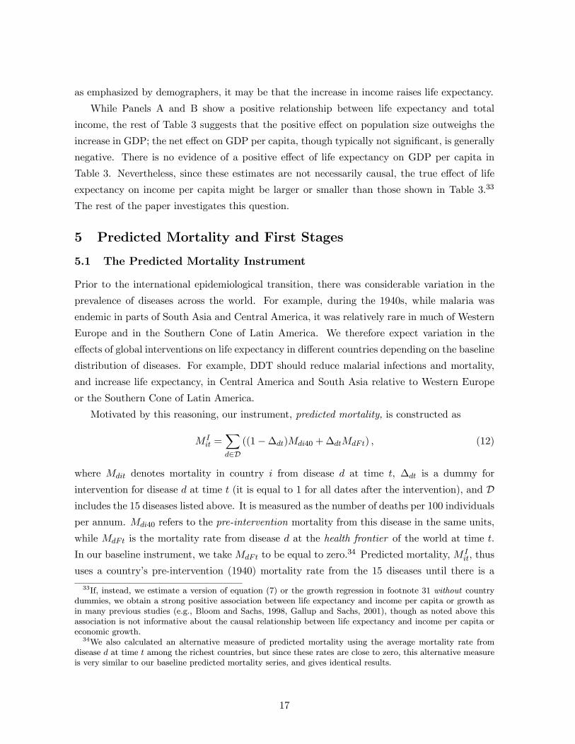
as emphasized by demographers, it may be that the increase in income raises life expectancy.

While Panels A and B show a positive relationship between life expectancy and total

income, the rest of Table 3 suggests that the positive effect on population size outweighs the

increase in GDP; the net effect on GDP per capita, though typically not significant, is generally

negative. There is no evidence of a positive effect of life expectancy on GDP per capita in

Table 3. Nevertheless, since these estimates are not necessarily causal, the true effect of life

expectancy on income per capita might be larger or smaller than those shown in Table 3.33

The rest of the paper investigates this question.

5 Predicted Mortality and First Stages

5.1 The Predicted Mortality Instrument

Prior to the international epidemiological transition, there was considerable variation in the

prevalence of diseases across the world. For example, during the 1940s, while malaria was

endemic in parts of South Asia and Central America, it was relatively rare in much of Western

Europe and in the Southern Cone of Latin America. We therefore expect variation in the

effects of global interventions on life expectancy in different countries depending on the baseline

distribution of diseases. For example, DDT should reduce malarial infections and mortality,

and increase life expectancy, in Central America and South Asia relative to Western Europe

or the Southern Cone of Latin America.

Motivated by this reasoning, our instrument, predicted mortality, is constructed as

MIit =

Xd∈D

((1−∆dt)Mdi40 +∆dtMdFt) , (12)

where Mdit denotes mortality in country i from disease d at time t, ∆dt is a dummy for

intervention for disease d at time t (it is equal to 1 for all dates after the intervention), and Dincludes the 15 diseases listed above. It is measured as the number of deaths per 100 individuals

per annum. Mdi40 refers to the pre-intervention mortality from this disease in the same units,

while MdFt is the mortality rate from disease d at the health frontier of the world at time t.

In our baseline instrument, we take MdFt to be equal to zero.34 Predicted mortality, M I

it, thus

uses a country’s pre-intervention (1940) mortality rate from the 15 diseases until there is a

33If, instead, we estimate a version of equation (7) or the growth regression in footnote 31 without countrydummies, we obtain a strong positive association between life expectancy and income per capita or growth asin many previous studies (e.g., Bloom and Sachs, 1998, Gallup and Sachs, 2001), though as noted above thisassociation is not informative about the causal relationship between life expectancy and income per capita oreconomic growth.34We also calculated an alternative measure of predicted mortality using the average mortality rate from

disease d at time t among the richest countries, but since these rates are close to zero, this alternative measureis very similar to our baseline predicted mortality series, and gives identical results.

17

global intervention, and after the global intervention, the mortality rate from the disease in

question declines to the frontier mortality rate.

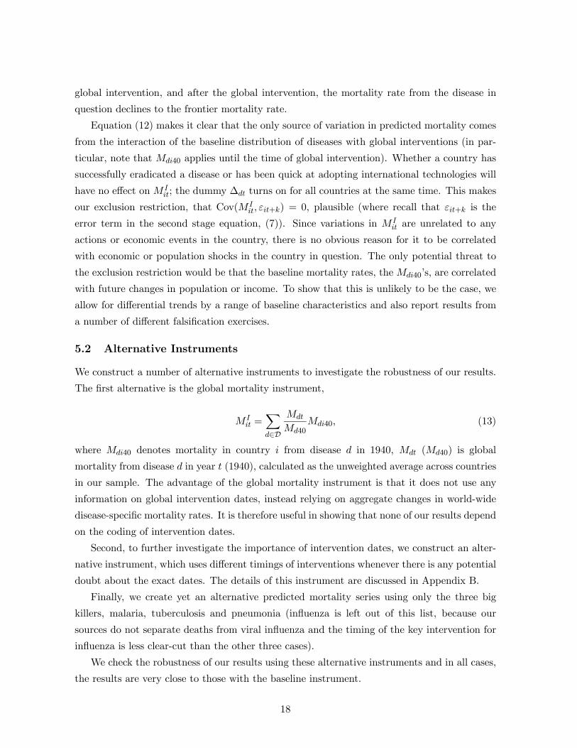
Equation (12) makes it clear that the only source of variation in predicted mortality comes

from the interaction of the baseline distribution of diseases with global interventions (in par-

ticular, note that Mdi40 applies until the time of global intervention). Whether a country has

successfully eradicated a disease or has been quick at adopting international technologies will

have no effect on M Iit; the dummy ∆dt turns on for all countries at the same time. This makes

our exclusion restriction, that Cov(M Iit, εit+k) = 0, plausible (where recall that εit+k is the

error term in the second stage equation, (7)). Since variations in MIit are unrelated to any

actions or economic events in the country, there is no obvious reason for it to be correlated

with economic or population shocks in the country in question. The only potential threat to

the exclusion restriction would be that the baseline mortality rates, the Mdi40’s, are correlated

with future changes in population or income. To show that this is unlikely to be the case, we

allow for differential trends by a range of baseline characteristics and also report results from

a number of different falsification exercises.

5.2 Alternative Instruments

We construct a number of alternative instruments to investigate the robustness of our results.

The first alternative is the global mortality instrument,

M Iit =

Xd∈D

Mdt

Md40Mdi40, (13)

where Mdi40 denotes mortality in country i from disease d in 1940, Mdt (Md40) is global

mortality from disease d in year t (1940), calculated as the unweighted average across countries

in our sample. The advantage of the global mortality instrument is that it does not use any

information on global intervention dates, instead relying on aggregate changes in world-wide

disease-specific mortality rates. It is therefore useful in showing that none of our results depend

on the coding of intervention dates.

Second, to further investigate the importance of intervention dates, we construct an alter-

native instrument, which uses different timings of interventions whenever there is any potential

doubt about the exact dates. The details of this instrument are discussed in Appendix B.

Finally, we create yet an alternative predicted mortality series using only the three big

killers, malaria, tuberculosis and pneumonia (influenza is left out of this list, because our

sources do not separate deaths from viral influenza and the timing of the key intervention for

influenza is less clear-cut than the other three cases).

We check the robustness of our results using these alternative instruments and in all cases,

the results are very close to those with the baseline instrument.

18

5.3 Zeroth-Stage Estimates

Our approach is predicated on the notion that global interventions reduce mortality from vari-

ous diseases. Therefore, before documenting the first-stage relationship between our predicted

mortality measure and log life expectancy, we show the effect of various global interventions

on mortality from specific diseases. In this exercise, in addition to the 15 diseases above, we

also use deaths from cancers and malignant tumors as control diseases, since these were not

affected by the global interventions.

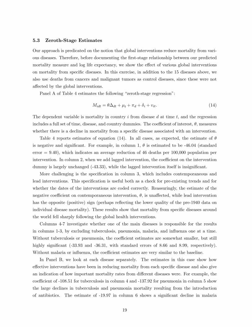
Panel A of Table 4 estimates the following “zeroth-stage regression”:

Midt = θ∆dt + µt + πd + δi + vit. (14)

The dependent variable is mortality in country i from disease d at time t, and the regression

includes a full set of time, disease, and country dummies. The coefficient of interest, θ, measures

whether there is a decline in mortality from a specific disease associated with an intervention.

Table 4 reports estimates of equation (14). In all cases, as expected, the estimate of θ

is negative and significant. For example, in column 1, θ is estimated to be -46.04 (standard

error = 9.40), which indicates an average reduction of 46 deaths per 100,000 population per

intervention. In column 2, when we add lagged intervention, the coefficient on the intervention

dummy is largely unchanged (-43.33), while the lagged intervention itself is insignificant.

More challenging is the specification in column 3, which includes contemporaneous and

lead interventions. This specification is useful both as a check for pre-existing trends and for

whether the dates of the interventions are coded correctly. Reassuringly, the estimate of the

negative coefficient on contemporaneous intervention, θ, is unaffected, while lead intervention

has the opposite (positive) sign (perhaps reflecting the lower quality of the pre-1940 data on

individual disease mortality). These results show that mortality from specific diseases around

the world fell sharply following the global health interventions.

Columns 4-7 investigate whether one of the main diseases is responsible for the results

in columns 1-3, by excluding tuberculosis, pneumonia, malaria, and influenza one at a time.

Without tuberculosis or pneumonia, the coefficient estimates are somewhat smaller, but still

highly significant (-33.93 and -36.31, with standard errors of 8.66 and 8.99, respectively).

Without malaria or influenza, the coefficient estimates are very similar to the baseline.

In Panel B, we look at each disease separately. The estimates in this case show how

effective interventions have been in reducing mortality from each specific disease and also give

an indication of how important mortality rates from different diseases were. For example, the

coefficient of -108.51 for tuberculosis in column 4 and -137.92 for pneumonia in column 5 show

the large declines in tuberculosis and pneumonia mortality resulting from the introduction

of antibiotics. The estimate of -19.97 in column 6 shows a significant decline in malaria

19

mortality, but the lower magnitude of this number indicates that mortality from malaria was

less important for our entire sample than mortality from tuberculosis or pneumonia (partly

because large areas of the world were not affected by malaria). The declines in mortality

from the other diseases are even smaller, but with the exception of influenza and measles (not

shown), they are always statistically significant.

5.4 First-Stage Estimates

We next turn to the first-stage relationship between life expectancy and predicted mortality.

While the zeroth-stage regression in equation (14) is at the disease-country-time level, our

first-stage relationship is at the country-time level, since the left-hand side variable is life

expectancy (at birth).

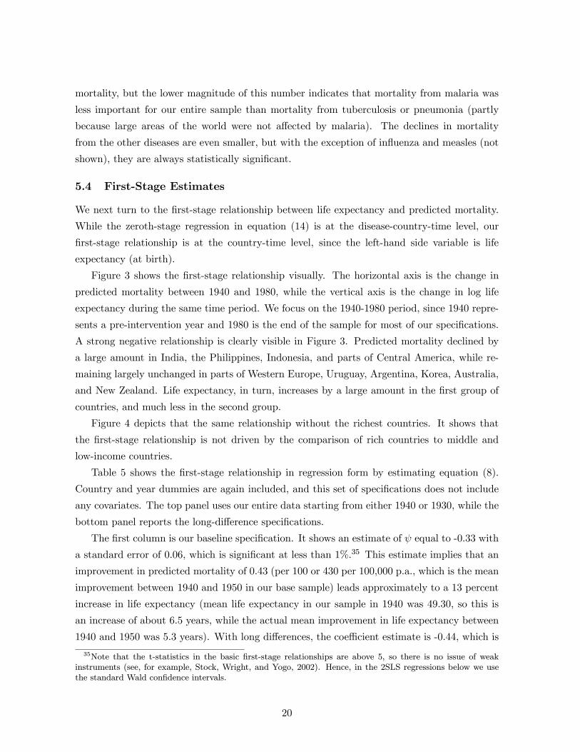
Figure 3 shows the first-stage relationship visually. The horizontal axis is the change in

predicted mortality between 1940 and 1980, while the vertical axis is the change in log life

expectancy during the same time period. We focus on the 1940-1980 period, since 1940 repre-

sents a pre-intervention year and 1980 is the end of the sample for most of our specifications.

A strong negative relationship is clearly visible in Figure 3. Predicted mortality declined by

a large amount in India, the Philippines, Indonesia, and parts of Central America, while re-

maining largely unchanged in parts of Western Europe, Uruguay, Argentina, Korea, Australia,

and New Zealand. Life expectancy, in turn, increases by a large amount in the first group of

countries, and much less in the second group.

Figure 4 depicts that the same relationship without the richest countries. It shows that

the first-stage relationship is not driven by the comparison of rich countries to middle and

low-income countries.

Table 5 shows the first-stage relationship in regression form by estimating equation (8).

Country and year dummies are again included, and this set of specifications does not include

any covariates. The top panel uses our entire data starting from either 1940 or 1930, while the

bottom panel reports the long-difference specifications.

The first column is our baseline specification. It shows an estimate of ψ equal to -0.33 with

a standard error of 0.06, which is significant at less than 1%.35 This estimate implies that an

improvement in predicted mortality of 0.43 (per 100 or 430 per 100,000 p.a., which is the mean

improvement between 1940 and 1950 in our base sample) leads approximately to a 13 percent

increase in life expectancy (mean life expectancy in our sample in 1940 was 49.30, so this is

an increase of about 6.5 years, while the actual mean improvement in life expectancy between

1940 and 1950 was 5.3 years). With long differences, the coefficient estimate is -0.44, which is

35Note that the t-statistics in the basic first-stage relationships are above 5, so there is no issue of weakinstruments (see, for example, Stock, Wright, and Yogo, 2002). Hence, in the 2SLS regressions below we usethe standard Wald confidence intervals.

20

somewhat larger, but also slightly less precisely estimated (standard error = 0.09).

Results are similar for 1930-1980 in column 2 (and also for 1940-1970 or 1930-1970–not

reported in the table). Column 3 shows analogous results when we include Eastern Europe.

Column 4 excludes the initially rich countries and shows a statistically significant (though

smaller) estimate of ψ (e.g., -0.23 with a standard error of 0.08 in Panel A).

Our baseline sample consists of an unbalanced panel. Column 5 shows that limiting the

sample to a balanced panel makes little difference. The estimate of ψ is now -0.32 (standard

error = 0.06).

Columns 6-8 investigate the robustness of the first stage to the inclusion of a range of inter-

actions between country-specific variables and time dummies; these specifications are therefore

similar to equation (10) above, except that they include interactions with initial values of insti-

tutions, log GDP per capita and continent dummies. For example, column 6 allows countries

with different institutions (as measured by average constraint on the executive, from the Polity

IV dataset, in 1950, 1960, and 1970) to have different changes in life expectancy in every year.

This has little effect on the baseline estimates, which are now -0.27 (standard error = 0.07)

in Panel A and -0.35 (standard error = 0.09) in Panel B. Column 7 includes interactions with

initial (1930) log GDP per capita, flexibly allowing for differential trends in life expectancy

for countries starting with different levels of prosperity. This also has very little effect on the

estimates. Column 8 includes a full set of interactions between continent dummies and life

expectancy, to control for the potential differential impact of distinct disease environments on

the evolution of life expectancy. Once again, this has very little effect on the estimates, which

remain highly significant and very close to the baseline.

Columns 9—12 investigate robustness to alternative instruments. Columns 9 and 10 use the

global mortality instrument for the base sample and for the sample including only initially low

and middle-income countries. The estimates are slightly larger and more significant.36 For

example, in Panel A the estimate of ψ is -0.41 (standard error = 0.08). Column 11 uses the

alternative timing of global interventions as described in Appendix B, again with very similar

estimates. These results show that the exact coding of global interventions and whether we

use aggregate trends in disease-specific mortality or information on global interventions have

little effect on the first-stage relationship. Finally, column 12 shows very similar results when

the instrument uses information from only tuberculosis, malaria and pneumonia.

Overall, the results in Table 5 show a large and robust effect of the predicted mortality

instrument on life expectancy. We next investigate the robustness of these results further.

36The exception is column 10 in Panel B, where the estimate is significant only at 10%.

21

5.5 Further Robustness Checks

Appendix Table C1 investigates the importance of disease composition to see whether a specific

disease is responsible for the first-stage relationships shown in Figures 4 and 5 and in Table 5.37

Columns 2, 3 and 4 of this table present results dropping data on the three main killers from

our predicted mortality measure: tuberculosis, malaria and pneumonia respectively. Dropping

tuberculosis or pneumonia strengthens the first stage estimates slightly, while none of the other

diseases has a significant impact on the first stage coefficient. We conclude from these results

that the first-stage relationship does not reflect the impact of any single disease.

The specifications in Table 5 do not allow for mean reversion in life expectancy, and also

assume that it is contemporaneous predicted mortality that affects life expectancy. Failure to

correctly specify the mean-reverting dynamics in life expectancy may bias our results. More-

over, in more general specifications we may find that it is lags or leads of predicted mortality

that affect life expectancy. In particular, if it is the leads of (future changes in) predicted mor-

tality that affect life expectancy, this would shed doubt on our interpretation of the first-stage

relationship. Table 6 investigates these issues. Column 1 repeats our baseline specification

(from column 1 of Table 5). Column 2 reports OLS estimates from the following model:

xit = νxit−1 + ψM Iit + δ0i + µ0t + uit, (15)

which allows lagged log life expectancy to affect current log life expectancy. There is indeed

evidence for mean reversion; the coefficient ν in the top panel is estimated to be 0.44 (standard

error = 0.09). Nevertheless, the negative relationship between predicted mortality and life

expectancy remains. The parameter of interest, ψ, is now estimated at -0.18 (standard error =

0.08), and implies a long-run impact similar to that in our baseline specification (the long-run

impact in this case is 0.18/ (1− 0.44) ≈ 0.32).Because we have a relatively short panel, OLS estimation of (15) will lead to inconsistent

estimates. To deal with this problem, we follow the method of Anderson and Hsiao (1992) in

column 3. This involves first-differencing (15), to obtain:

∆xit = ν∆xit−1 + ψ∆M Iit +∆µ

0t +∆uit,

where the fixed country effects are removed by differencing. Although this equation cannot be

estimated consistently by OLS either, in the absence of serial correlation in the original residual,

uit, there will be no second order serial correlation in ∆uit, so xit−2 will be uncorrelated with

∆uit and can be used as instrument for ∆xit−1 to obtain consistent estimates. SimilarlyMIit−1

is used as an instrument for ∆M Iit. This procedure leads to very similar results to the OLS

estimates. The estimate of ψ is -0.27 (standard error = 0.14).

37Appendix Tables C1-C4 are included in Appendix C and are not for publication.

22

Although the instrumental variable estimator of Anderson and Hsiao (1982) leads to con-

sistent estimates, it is not efficient, since, under the assumption of no serial correlation in uit,

not only xit−2, but all earlier lags of xit in the sample are also uncorrelated with ∆uit, and

can also be used as additional instruments. Arellano and Bond (1991) develop a Generalized

Method-of-Moments (GMM) estimator using all of these moment conditions. When all these

moment conditions are valid, this GMM estimator is more efficient than Anderson and Hsiao’s

(1982) estimator. GMM estimation, which we use in column 4, leads to similar but more

precisely estimated coefficients. The estimate of ψ in the full sample is now -0.19 (standard

error = 0.06). Tests for second-order autocorrelation in the residuals, reported at the bottom

of the column, show that there is no evidence of additional serial correlation. However, the

Hansen J-test shows that the overidentification restrictions are rejected, presumably because

different lags of life expectancy lead to different estimates of the mean reversion coefficient.

This rejection is not a major concern for our empirical strategy since the exact magnitude of

the mean reversion coefficient, ν, is not of direct interest to us. Essentially because the models

in (8) and (15) are the first stage in our 2SLS procedure, all we need is for M Iit−1 not to have

a direct effect on the second-stage outcomes.

Columns 5-7 investigate the effect of lagged and lead mortality. In column 5, contem-

poraneous and lagged mortality are included together. Not surprisingly, both of these are

significant, since, in many countries, global health interventions were implemented gradually

over time (recall that an intervention is coded at the time of the major global breakthrough).

The more important challenge for our approach is the inclusion of lead predicted mortality.

Since global interventions did not start before 1940, lead mortality should have no effect on

life expectancy. Column 6 investigates this by including contemporaneous and lead mortality

together. In this case, the estimate of the effect of contemporaneous predicted mortality is

-0.33 (standard error = 0.06), while lead mortality is not significant and has the wrong sign.

Column 7 includes contemporaneous, lag, and lead predicted mortality together, and in this

case both contemporaneous and lag mortality are statistically significant, while lead mortality

remains highly insignificant. These results suggest that, consistent with our hypothesis, it was

indeed the global interventions of the 1940s onwards that led to the increase in life expectancy

in countries previously affected by these diseases.

Finally, columns 8 and 9 shows that controlling for the effect of income per capita has little

impact on the relationship between predicted mortality and life expectancy, and column 10

shows very similar to our baseline estimates from the balanced panel of countries.

23

5.6 Pre-Existing Trends and Falsification

Table 6 already showed that life expectancy responds to contemporaneous changes in predicted

mortality and does not respond to future changes. This suggests that our first stage is unlikely

to be driven by pre-existing trends. Nevertheless, the exercise in Table 6 uses only data from

1940 onwards. An alternative falsification exercise on pre-existing trends is to look at changes

in life expectancy during the pre-period, 1900-1940, and see whether they correlate with future

(post-1940) changes in predicted mortality. This is done in Figures 5 through 8 and in Table

7.

Figure 5 shows the change in log life expectancy 1900-1940 against the change in predicted

mortality 1940-1980. There is no evidence of a negative relationship similar to those in Figures

3 and 4. In fact, there is a slight positive slope (which is statistically insignificant–see Table

7). Figure 6 shows the same relationship without the richest countries, and there is now a

somewhat stronger positive relationship (again insignificant–see Table 7). There is thus no

evidence of pre-existing trends that could explain our first-stage results.

Figures 7 and 8 substantiate the patterns in Figures 5 and 6 further by showing changes

in log life expectancy just before the international epidemiological transition, between 1930

and 1940 against the predicted mortality instrument. These figures also show no evidence of

a significant negative relationship either for the whole sample or for the subsample excluding

the initially richest countries. Our measure of predicted mortality explains changes in life

expectancy after 1940 but not before 1940.

Table 7 also extends our examination of potential pre-existing trends to the outcome mea-

sures, by looking for a potential relationship between our measure of post-1940 predicted

mortality and changes in log population, log GDP, and log GDP per capita between 1900 and

1940.38 Columns 1 and 2 confirm the positive and insignificant relationship between change in

predicted mortality between 1940 and 1980 and change in life expectancy between 1900 and

1940 shown in Figures 5 and 6. Columns 3 and 4 show that there are no differential pre-existing

trends in log population between 1900 and 1940 either for the entire sample or for the sample

excluding the richest countries. Columns 5-8 show similar results for log GDP and log GDP

per capita.

These results therefore indicate that there were no pre-existing trends in life expectancy or

in our key outcome variables prior to the international epidemiological transition.39 This gives

us greater confidence in using predicted mortality as an instrument to investigate the effect of

38We do not have enough data to do this for total births. Data limitations also make our sample sizes for theother variables smaller for this exercise than for our main regressions.39For a more qualitative confirmation that there was no pre-existing trend, see Carr-Saunders (1936). In this

comprehensive review of population trends, there is no hint of the increase in life expectancy and populationthat was to occur shortly.

24

life expectancy on a range of economic outcomes.

Finally, we further use Table 7 to show the reduced-form relationships between predicted

mortality and some of our outcome variables. Recall that life expectancy is a proxy for overall

health of the population, so the reduced-form relationships between predicted mortality and

the outcome variables are as informative as the 2SLS estimates reported below. Panel B

of Table 7 shows these reduced-form relationships. As already shown, there is a significant

negative relationship between life expectancy and predicted mortality in the period 1940-

80. In addition, there is a significant negative relationship between predicted mortality and

population during the same period, which indicates an increase in population in previously

high-mortality areas resulting from the international epidemiological transition. The other

columns show a negative but insignificant relationship between predicted mortality and total

GDP, and a positive relationship between predicted mortality and GDP per capita. These

results imply that declines in mortality were associated with lower GDP per capita (since total

GDP did not increase much and population grew substantially). The 2SLS estimates presented

in the next section confirm these reduced-form relationships.

6 Main Results

We now present our main results, which are the 2SLS (two-stage least square) estimates of

the effect of log life expectancy on six outcome variables: log population, log total births, log

GDP, log GDP per capita, log GDP per working age population, and years of schooling.

For each outcome we use two estimation strategies. The first is a full panel with decadal

observations between 1940 and 1980, while the second looks only at the long difference using

data from 1940 and 1980. The tables have a parallel structure (except for schooling, where data

availability makes this impossible). In addition, in each case, we look both for contemporaneous

effects and for “longer-run” effects after 10, 20, 30, and 40 years.

6.1 Population

Figure 9 shows a strong negative reduced-form relationship between change in log population

1940-80 and the change in predicted mortality over the same period. This pattern, already

seen in Panel B of Table 7, implies that countries with a larger decline in predicted mortality

experienced a larger increase in log population, i.e., more population growth. Given the neg-

ative relationship between predicted mortality and life expectancy in Figure 4, this translates

into a positive effect of life expectancy on population. This is confirmed in Table 8, which

reports 2SLS results from regressing log population on log life expectancy in either a panel

specification (Panel A) or in long differences (Panel B). The first stages for these regressions

are reported in Table 5 and are not repeated here to save space.

25

In column 1 we look at contemporaneous effects during 1940-80 and find a coefficient on

log life expectancy of 1.31, with a standard error of 0.37 (statistically significant at 1%). This

estimate is comparable to the OLS estimates in Table 2.

The coefficient increases to 1.35 when we look at 1930-80 (column 2) and is even larger

when we include Eastern Europe (column 3). When we exclude the initially richest countries

in column 4, the coefficient estimate is again similar, 1.58 (standard error = 0.76).

Column 5 shows that the results are generally robust (though slightly smaller) when we

include the full set of interactions between year dummies and institutions (both in the first and

second stages).40 These interactions are jointly significant, suggesting that initial institutional

differences have some predictive power for subsequent population growth. Column 6 estimates

equation (10), allowing for a full set of interactions between year dummies and initial (1930)

log population. As noted above, this specification flexibly controls for both mean reversion and

potential differential trends. Remarkably, the estimate of the effect of log life expectancy on log

population is essentially unaffected, 1.33 (standard error = 0.35), though interactions between

year dummies and initial population are jointly statistically significant. The corresponding

estimate in Panel B is also very similar to the baseline, 1.68 (standard error = 0.44).

Column 7 repeats the baseline regression using the global mortality instrument. In Panel

A, the estimate of the effect of log life expectancy on log population is 1.65 (standard error =

0.40), while in Panel B, it is 1.70 (standard error = 0.48).

Columns 8-11 investigate the longer-term effects of life expectancy on population growth

by looking at the specifications where the dependent variable is various leads of log population

(i.e., k > 0 in terms of equation (7)). The coefficients are on the whole very similar to the

baseline estimate (slightly higher for 10 and 20 year leads and slightly smaller for the 40 year

lead). This suggests that changes in life expectancy led to relatively enduring increases in

population. Panel B shows the same results with the long difference specifications.

Overall, we find a large, relatively precise, and robust effect of life expectancy on population.

The elasticity is estimated consistently to lie between 1 and 2, which is similar to the OLS

estimates.

6.2 Births

Table 9 presents 2SLS estimates of log life expectancy on log total births. Consistent with the

magnitude of the response of population to life expectancy, Table 9 indicates that the increase

in life expectancy was associated with an increase in the total number of births. In column 1,

Panel A, the estimate is 2.39 (standard error = 0.69). The estimates are similar in the long-

difference specifications, when we include Eastern Europe, when we exclude the initially richest

40The results including the interactions between year dummies and initial log GDP per capita or continentdummies are also very similar and are not reported to save space.

26

countries, when we include interactions between year dummies and institutions, or initial log

GDP per capita, continent dummies, and initial log total births, and when we use the global

mortality instrument.

Looking at the leads shows an interesting pattern whereby the effects become smaller at

future dates. This suggests that there was a delayed decline in fertility in response to the

increase in life expectancy (which is consistent with the evidence reviewed in Kelley, 1988).

6.3 GDP

Figure 10 shows the reduced-form relationship between change in log (total) GDP and change

in predicted mortality during 1940-1980. Consistent with the pattern in Panel B of Table 7,

there is a slight (but not statistically significant) downward slope, which indicates that countries

with larger declines in predicted mortality experienced somewhat higher GDP growth between

1940 and 1980, though this effect is not very large.

Table 10 presents the related 2SLS regression evidence. In column 1, the estimate of the

key parameter is -0.03 (standard error = 0.67). The estimate using long differences in Panel

B (corresponding to Figure 10) is positive, 0.32, but also statistically insignificant (standard

error = 0.84). In both cases, the standard errors are large enough that economically significant

positive effects cannot be ruled out. For example, the two standard error (95% confidence)

intervals always include a response of GDP to life expectancy with an elasticity that could be

as high as 1.3. Nevertheless, the standard errors will be somewhat smaller when we look at

GDP per capita below, enabling us to exclude any positive effects on per capita growth.

The pattern of response of GDP to life expectancy is broadly similar when we look at dif-

ferent sample periods, when we include Eastern Europe, exclude the initially richest countries,

when we include interactions between year dummies and institutions or initial GDP per capita,

and when we use the global mortality instrument.

The estimates in columns 8-11 show that at longer horizons there is a more positive effect

of life expectancy on GDP (though still not significant). For example, with the 10-year lead the

coefficient is now 0.52 (standard error = 0.48) and with the 20-year lead it is 0.53 (standard

error = 0.44). The effect starts declining after the 30-year lead. Estimates using the long

differences are close to and somewhat larger (though considerably less precise) than the panel

estimates in Panel A. The over-time increase in the impact of life expectancy on GDP could be

a result of a combination of the larger population reaching working age, and consistent with

the neoclassical growth model, capital inputs and other factors of production adjusting to the

increase in population.

We interpret these estimates as suggesting that the increase in life expectancy and the

associated increase in population had a relatively small effect on total GDP at first, with a

27

somewhat larger effect over time. Nevertheless, the relatively large standard errors make it

impossible for us to pin down the exact magnitude or timing of the impact of life expectancy

on total GDP.

6.4 GDP Per Capita and Per Working Age Population

The response of total GDP already reveals that the effect of the increase in life expectancy

on GDP per capita (or GDP per working age population) was negative. This is shown in

Figure 11, which depicts a strong positive reduced-form relationship between the change in log

GDP per capita and the change in predicted mortality during 1940-1980. Evidently, countries

with larger declines in predicted mortality also experienced lower growth in GDP per capita.

Clearly, this is the result of the larger increase in population than in GDP in these countries,

which was already shown in Figures 11 and 12 and in Panel B of Table 7.

The 2SLS estimates of the effect of log life expectancy on GDP per capita in Table 11

confirm this pattern. There is a significant negative effect of life expectancy on GDP per

capita in columns 1 and 2 of Panels A and B. In either case, the coefficient estimate for π in

equation (7) is around -1.30 (with standard errors ranging between 0.46 and 0.61).

The results in columns 3-6, which look at alternative samples and include interactions with

initial institutions and initial log GDP per capita, are similarly negative and hover around

statistical significance. Estimates from equation (10) in column 7, on the other hand, lead to

still negative but smaller effects of log life expectancy on GDP per capita. In all cases, the two

standard error bands always exclude positive effects of life expectancy on GDP per capita.

As with the results for total GDP in Table 10, the lead results indicate a more positive (less

negative) impact of life expectancy on GDP per capita over the following 40 years than initially.

Nevertheless, even after 40 years, there is no evidence of a positive effect of life expectancy on

GDP per capita.

One concern with these results is that the increase in population is largely at young ages,

so GDP per capita may be low precisely because the denominator has increased, while the

working age population has not. To investigate the importance of this issue, Appendix Table

C2 looks at GDP per working age population,41 and shows that the impact of life expectancy

on GDP per working age population is very similar to its impact on GDP per capita.

Overall, our 2SLS estimates show no evidence that the large increase in life expectancy in

many parts of the world starting in the 1940s led to a significant increase in GDP per capita.42

Instead, the increase in life expectancy was associated with a significant increase in population

41We define working age population as population between the ages of 15 and 60. Estimates of the agedistribution of the population and hence of the working age population for this time period are often rough.42As noted in footnote 40, the results are similar when we control for a full set of continent dummies interacted

with time. For example, in the specification of Table 11, the coefficient on log life expectancy is -0.27 (standarderror = 0.45).

28

and a somewhat smaller increase in total GDP.

These results are broadly consistent with the neoclassical growth model. In terms of the

model in Section 2, suppose that the contemporaneous effects correspond to the “medium

run” impact with the capital stock held constant. The coefficient of interest, in this case,

is π = (α (γ + η)− (1− α)λ) in terms of equation (6). Recall that λ here is the response of

population to changes in life expectancy, so according to the estimates in Table 8, we can think

of λ ≈ 1.5. The coefficient α corresponds to the share of labor. Since the countries in questionhere include many low-income countries where land is an important factor of production, we

take the share of land as 1/3, i.e., 1 − α − β ≈ 1/3 (see footnote 13), and thus set α ≈ 1/3and β ≈ 1/3. This would imply that our estimate of π = (α (γ + η)− (1− α)λ) ≈ −1.3is consistent with γ + η close to zero or even slightly negative. If, on the other hand, we

were to take λ to be around 1.7 as suggested by the high-end estimates in Table 8, γ + η

would be small but positive.43 Therefore, these results suggest that the benefits of higher

life expectancy in terms of direct productivity gains and human capital gains are relatively

small. This is also confirmed when we look at the longer-run effects. For example, if we take

the long-run effect to be approximately -0.75 and β ≈ 1/3, then the long-run relationship

of π = (α (γ + η)− (1− α− β)λ) / (1− β) implies a value of γ + η equal to zero. Smaller

negative effects, which are within the two standard error bands of the estimates in Table 11,

would be consistent with positive values of γ + η.44

6.5 Years of Schooling

The results so far do not show any evidence of large gains from increases in life expectancy

in terms of economic growth per capita. Instead, the greater population associated with the

increase in life expectancy appears to have somewhat reduced income per capita. This suggests

that the indirect benefits of improved health in terms of greater education and greater (total

factor) productivity may be limited (see the calculations in the last paragraph of the previous

subsection). As a further check on this conclusion and as a way of investigating whether there

are any substantial effects of life expectancy working through human capital (as posited by

equation (4)), we can also directly look at whether increasing life expectancy raised human

capital during and in the aftermath of the international epidemiological transition.

Table 12 estimates the corresponding 2SLS regressions using the available data on schooling

starting in 1960. Data availability implies that we can only look at the effect of life expectancy

43But in turn, if α were higher, the implied values of γ + η would be correspondingly lower. For example,Hansen and Prescott (2002) suggest a value of 0.3 for 1−α−β, 0.1 for β and 0.6 for α in pre-industrial societies.44The comparison of these results to the OLS estimates in Table 3 (together with the pattern discussed in

footnote 32) suggests that the lack of a significant OLS relationship between life expectancy and GDP per capitais likely to be due to a combination of a short-run negative effect of life expectancy on GDP per capita and apositive effect of income on life expectancy. See also Pritchett and Summers (1998) for estimates of income percapita on life expectancy.

29

on 10-year or 20-year leads of schooling (which is not a severe limitation since there are likely

to be important lags in the effect of life expectancy on schooling). The results in Table 12 show

that there is no effect of life expectancy on schooling in the OLS and in the IV either in the

base sample or for only low and middle-income countries (columns 1-6). With 30-year leads,

there is a positive and significant OLS estimate, but the IV estimates are again insignificant

(either positive or negative depending on the sample, as shown in columns 8 and 9).

Overall, there seems to be no evidence that the increase in life expectancy has been as-

sociated with substantially greater investment in human capital, which is consistent with the

finding in the previous subsection. The most likely reason why the increase in life expectancy

did not translate into greater education during this episode is that the affected countries faced

bottlenecks in their education systems, making it impossible for them to increase the edu-

cation of the much larger cohorts of children that survived and were born as a result of the

international epidemiological transition.

7 Further Results

The results in the previous section suggest that the increase in life expectancy led to a sub-

stantial increase in population, but not to more rapid economic growth. In this section, we

investigate the robustness of these results further.

7.1 Alternative Samples

An important question is whether including sub-Saharan Africa in the analysis changes any of

the main results documented above. This is hard to answer with great certainty as the detailed

data for Africa before at least 1950 are either not available or not reliable. Although there is

a sizable historical literature on medical conditions in Africa, much of this is not accompanied

by statistics that are comparable with our base sample data.45 Nevertheless, it is possible to

include sub-Saharan Africa after 1950 in our regressions using UN data (which are nonetheless

less reliable than the non-African data, see Appendix C for details). This is done in columns

1-4 and 7-10 of Table 13. The results for the first and the second stages are similar to our

previous results both using the baseline and the global mortality instruments.46 In this case,

45In general terms, we know that health in Africa improved, at least for a while after World War II. Forexample, Cutler et al (2006, p. 17) write: “life expectancy [in Africa] rose by more than 13 years from the early1950s to the late 1980s, before declining in the face of HIV/AIDS.” Estimates in Gwatkin (1980, e.g., Figure 2)also suggest that increases in life expectancy were at least as dramatic in Africa as in other developing countries,but only until average life expectancy for these societies reached 40; at that point the rate of increase slowedsharply. This could point to a failure to sustain health improvements or some other factor, and needs furtherinvestigation.46The sample used here is limited both by lack of life expectancy data in 1940 and by the fact that Maddison

does not have population or GDP data for Africa before 1950. Consequently, even though Table 13 usesinformation on 43 more countries than the previous tables, the additional observations are all post-1950.

30

estimates using the global mortality instrument are more reliable since they do not use the

baseline disease distributions in Africa.

A second alternative sample drops countries that were demographically most affected by

World War II. Urlanis (2003) documents demographic effects that were both direct, through

loss of population, and indirect, through reducing birth rates and increasing non-casualty death

rates in a number of countries. Interestingly, however, in relatively few cases was there a first-

order effect on population. Based on Urlanis (2003), columns 5-6 and 11-12 of Table 13 report

results dropping Germany, Italy, Finland, Austria, and China (Japan is not in our sample

due to data issues; Eastern Europe is not in the baseline sample). The first-stage relationship

between log life expectancy and predicted mortality remains strong and highly significant, and

there is again a large effect on population and a smaller, insignificant effect on total GDP.

We also estimated regressions dropping countries that were involved in developing the

new “miracle” drugs and chemicals of the 1940s and 1950s: the UK, the US, Germany and

Switzerland. For these countries one might be concerned that the medical innovations were

partly endogoneous to their disease conditions. In any case, this has hardly any effect on the

estimates (not reported).

7.2 Mean Reversion in the Second Stage

In Appendix Table C3, for our main variable of interest, income per capita, we estimate a

version of equation (9), which explicitly allows for mean reversion in the dependent variable.

Recall that the presence of such mean reversion does not affect the consistency of the esti-

mates presented so far as long as our instrument for life expectancy is valid (i.e., as long as

Cov(MIit, εit+k) = 0), so we report these estimates mostly for completeness.

Our strategy is to estimate a transformed model that removes the effect of mean reversion

in income per capita. Suppose we know the mean-reversion parameter ρ in equation (9). Then,

subtract ρyit−1 from yit, which, using (9) without covariates, gives

yρit = πxρit + ζρi + µρt + ερit,

where the transformed dependent variable is yρit ≡ yit − ρyit−1, and on the right hand side we

have xρit ≡ xit−ρxit−1 (and ερit ≡ εit−ρεit−1). M Iit can be used as an instrument for x

ρit in this

equation (since Cov(M Iit, εit+k) = 0 for all k, we also have Cov(M

Iit, ε

ρit) = 0). Therefore, a 2SLS

regression of yρit on xρit will identify the coefficient of interest, π. Although we do not know ρ, we

can implement a two-stage version of this procedure by first estimating ρ.47 Appendix Table

C3 reports results from applying this procedure using a range of values for ρ that encompasses

(and exceeds) the range of estimates of ρ. There is a robust first stage between transformed

47In regressions of log income per capita on its lag and country and time fixed effects, the estimates of ρ varybetween 0.4 and 0.75 depending on estimation strategy and on whether or not log life expectancy is included.

31

log life expectancy and predicted mortality, and the second-stage estimates are similar to (but

somewhat more negative than) those in Table 11. These estimates show that irrespective of

the value of ρ, the relationship between life expectancy and GDP per capita is never positive

(the point estimate is always negative).

7.3 Interaction Results

As discussed in Section 2, we may expect the impact of log life expectancy on GDP per capita

to differ depending on the investment rate. We investigate this issue in Appendix Table C4

using two variables to measure investment rates: (1) initial (1930) log GDP per capita and (2)

investment rates from the 1940s (or immediately after). Although income differences in 1930

likely had various causes, we expect them to be correlated with savings and investment rates,

and these data are likely to be more reliable than estimates of investment rates around the

same time.

Our empirical strategy is to include an interaction between log life expectancy and initial

log GDP per capita or investment as a percent of GDP. This interaction term is instrumented

by the interaction between predicted mortality and initial log GDP per capita (or investment).

In all regressions, the main effects are evaluated at the sample mean. Panel A of Appendix

Table C4 shows that the effect of log life expectancy on population is the same irrespective of

initial log GDP p.c. or the investment rate; the interactions between log life expectancy and

these baseline characteristics are insignificant both in contemporaneous and lead specifications.

The picture is different in Panels B and C, where we look at log GDP and log GDP per

capita. In the regressions with contemporaneous effects, the interaction terms both with GDP

per capita in 1930 and investment share of GDP in 1940s are positive, and except for the

effect of the interaction with GDP per capita in 1930 on log total GDP (in Panel B), they

are statistically significant. For example, the coefficient on the interaction between GDP per

capita in 1930 and log life expectancy in the log GDP per capita regression (Panel C, column

1) is 0.79 (standard error = 0.37), while the interaction with investment share of GDP for the

same variable (Panel C, column 5) is 0.12 (standard error = 0.04). These estimates imply that,

consistent with our theoretical expectations, there is some evidence that countries with high

investment rates (measured directly or proxied by high initial income per capita) suffered less

adverse income effects from the increase in population. Moreover, consistent with equation

(5) in Section 2, these investment rate and life expectancy interactions appear not to have

had a positive impact on log GDP or log GDP per capita in the long run. Nevertheless, the

results of this exercise have to be interpreted with caution, since data quality and relatively

large standard errors limit the extent to which we can pin down the exact timing of changes

in GDP.

32

8 Conclusion

A newly-emerging consensus in academic and policy circles holds that disease environment and

health conditions lie at the root of large income differences across countries today, and argues

that improving health will not only improve lives but will by itself spur rapid economic growth.

This paper investigated these claims by estimating the effect of life expectancy at birth

on economic growth. The innovation in our approach is to exploit the international epidemi-

ological transition, which led to potentially-exogenous differential changes in mortality from a

number of major diseases across the world. As a result of new chemicals, drugs, and other in-

ternational interventions, mortality from tuberculosis, pneumonia, malaria, and various other

diseases declined sharply in many parts of the world, while other countries that were largely

unaffected by these diseases did not experience similar improvements in health and life ex-

pectancy. Exploiting these differential changes in predicted mortality as an instrument for life

expectancy, we estimate the effect of life expectancy on a range of economic variables, most

importantly population and GDP.

Our results indicate that the increase in life expectancy led to a significant increase in pop-

ulation; birth rates did not decline sufficiently to compensate for the increase in life expectancy.

We find a small initial positive effect of life expectancy on total GDP, and this effect grows

somewhat over the next 40 years, but not enough to compensate for the increase in population.

Overall, the increases in life expectancy (and the associated increases in population) appear

to have reduced income per capita at first, with this negative effect slowly wearing off over the

next 40 years. There is no evidence that the increase in life expectancy led to faster growth

of income per capita. This evidence sheds considerable doubt on the view that health has a

first-order impact on economic growth.

It is also important to emphasize the limitations of our results. The most important limi-

tation is that since our approach exploits the international epidemiological transition around

the 1940s, the results may not be directly applicable to today’s world. This is for at least two

reasons. First, the international epidemiological transition was a unique event and perhaps

similar changes in life expectancy today will not lead to an increase in population and the

impact on GDP per capita may be more positive. Second, the diseases that take many lives

in the poorer parts of the world today are not the same as those 60 years ago; most notably

HIV/AIDS is a major killer today but was not so in 1940. Most of the diseases we focus on had

the greatest impact on children (with the notable exception of tuberculosis), while HIV/AIDS

affects individuals at the peak of their labor productivity and could have a larger negative im-

pact on growth. Further study of the effects of the HIV/AIDS epidemic on economic outcomes

is an important area for future research.

33

9 Appendix A: Data Sources and Construction

Population, GDP, and GDP per capita data are from Maddison (2003), specifically the downloadabledata available to purchasers of his 2003 book. Working age population is defined as population be-tween the ages of 15 and 60 and is obtained from the on-line UN demographic database from 1950(http://esa.un.org/unpp). Population structure for 1940 is from the UN Demographic Yearbook 1948(United Nations 1949, Table 4, pp. 108-158). We use data for 1940 or the closest available year orrange of years. For 1930 we assume the same age structure as 1940 (this is relevant only for column 2of Appendix Table C2).

Life expectancy in 1940 and earlier are from various UN Demographic Yearbooks. Key Yearbooksare the original 1948 edition (United Nations 1949) and subsequent issues for 1949-50 (United Nations1950), for 1951 (United Nations 1951), and particularly the retrospective section of the DemographicYearbook 1967 (United Nations, 1967). We use the most recently revised UN data available to calculatethe unweighted averages of male and female life expectancy for 1940 (we also check these data againstUnited Nations, 2000, but the coverage of this generally begins no earlier than 1948). When there is nodata for 1940, but such data exist for neighboring years, e.g., 1938 and 1942, we use linear interpolationto obtain an estimate for 1940. In a few cases, we use information from neighboring countries when theyhave similar crude death rates (from the UN Demographic Yearbooks). Appendix C provides furtherdetails and gives the specifics for each country.

Life expectancy from 1950 onwards was downloaded from the on-line UN demographic database;these data are in five year intervals, so we use 1950-55 for 1950 and 1960-65 for 1960, etc. Life expectancyin 1900, used in the falsification tests, is from Maddison (2001, Table 1-5a, p. 30). These estimates forlife expectancy in 1900 for Europe, Latin America, and Asia are consistent with the numbers in Arriagaand Davis (1969), Riley (2001), and Bengtsson et al (2004).

To classify the cause of death, we use the Abridged List of the 1938 revision of the InternationalClassification of Disease. This list is comprehensive and has 44 categories. We omit any diseases thatare not infectious or could be degenerative, e.g., “diseases of the heart” (Abridged List No. 24) andresidual categories, such as “other infectious or parasitic diseases” (Abridged List No. 14). Syphilis(Abridged List No. 9) and puerperal fever/infection (Abridged List No. 35), which results from aninfection after childbirth, are omitted because their prevalence depends on sexual and fertility behavior,which fall outside our focus here. Finally, we further omit diseases that were never major causes ofdeath, even though they may have had serious effects on health (e.g., acute poliomyelitis). In all, thereare 15 infectious diseases for which we can obtain comparable cross-country data on deaths per 100,000in 1940 (or 1939 or a close year). Of these 15, 3 are reviewed in more detail in the main text and 12 arecovered in Appendix B. We have checked that the data we use in or around 1940 are not significantlyaffected by the impact of World War II; this is generally possible as in most cases some combination ofUnited Nations sources yields numbers for at least two early years. For European countries affected bythe war, we prefer data from 1937 or 1938, where available. Also, in our robustness checks, we drop alldata from countries where Urlanis (2003) deemed that war had a major demographic impact.

The classification of death rates by cause changed in 1948, and some of our data for 1950 and afterare available only according to the Abbreviated List, 1948 Revision of the International Classificationof Disease. For example, the UN Demographic Yearbook (1954) reports cause of death in and around1950 for some countries using the 1938 classification and for others using the 1948 classification. Theterminology of the Abridged List for the 1938 classification and the Abbreviated List for the 1948 clas-sification is as used in the Demographic Yearbook. Most of our 15 diseases can be tracked through thisreclassification, but dysentery/diarrhea-related diseases cannot–we have information on these diseasesonly for 1940 (which is what we need to construct the predicted mortality instrument), but they arenot included in our zeroth-stage regressions in Table 4 or in our calculation of the global mortalityinstrument.

For our data on cause of death in 1940, we start with the Summary of International Vital Statistics,1937-1944, published by the Federal Security Agency (1947) of the US government immediately afterWorld War II. This source provides comparable comprehensive data on cause of death around 1940, aswell as longer time series on the more important diseases (i.e., death rates by country), primarily from

34

League of Nations sources; however, it did not use all the available data (Federal Security Agency, 1947,p. 2). For this reason, we fill gaps for 1940 using the original sources, which are national health statisticscollected, cleaned and republished between the wars by the League of Nations Health Organization (seeFederal Security Agency, 1947, pp. 1-3); we also use information from the League and its direct postwarsuccessors for earlier and later data as discussed in Appendix C. A key issue is the area covered by theregistration of deaths in various countries. Apart from the very richest countries in 1940, there wasseldom universal registration of death, with a death certificate signed by a doctor. Consequently, someof the data are for major cities, while others are for all towns or for the entire population. Unfortunately,our sources do not always document clearly the precise coverage of the underlying data (for lower incomecountries, the data almost certainly overweigh towns relative to rural areas and diseases related to urbanovercrowding are likely to be overrepresented). Nevertheless, our results are robust to using only themore reliable data.

The League of Nations Health Organization established comparable international health statisticsfor a large number of countries, but never to our knowledge published a comprehensive retrospectiveof the data. Their first relevant publication was Issue No. 7 of the Annual Epidemiological Report,which appeared in October 1923. But only from 1929 (covering the year 1927) did this publicationinclude death rates from specific causes (League of Nations Health Organization, 1929). Early issuesof this publication are also refered to as Statistics of Notifiable Diseases. The first six issues focusedon Eastern Europe, particularly typhus and malaria epidemics in Russia. For a comprehensive list ofpublications by the League of Nations on health, see Aufricht (1951), particularly pp. 176-177. For anexplanation of the structure and purpose of the League of Nations Health Organization, see League ofNations (1931). For more on the early development of internationally comparable health statistics, seeStocks (1950).

We use the death rates by disease for 1930 from League of Nations Health Organization (1933).For 1940 we use World Health Organization (1951), which provided data for 1939-46, based on theLeague of Nations’ work. In addition, for malaria in 1930, we use data from the Leauge of Nations’Malaria Commission (League of Nations Health Organization, 1932). We also check our data againstinformation on location of malaria in the 1940s from American Geographical Society (1951a). Data ondeaths by disease for 1950 and 1960 are from the UN Demographic Yearbooks for 1954, 1962 and 1966.Data for 1970 are from the UN Demographic Yearbook for 1974 and data for 1980 are from the UNDemographic Yearbook for 1985.

We further confirmed that our data do not miss major epidemics by reviewing every available inter-war issue of the League of Nations’ Weekly Epidemiological Record. For example, for the distribution ofcholera in 1938, see Weekly Epidemiological Record, March 3rd, 1938. For the distribution of small poxin 1930, see Weekly Epidemiological Record, August 21st, 1930; for 1938, see Weekly EpidemiologicalRecord, March 3rd, 1938; for the early 1940s see Weekly Epidemiological Record, January 3rd, 1946.For the pre-war distribution of diphtheria, with a focus on Europe, see Weekly Epidemiological Record,December 21st, 1939. For the distribution of plague in 1938, see Weekly Epidemiological Record, March3rd, 1938. For more detail on the pre-1940 distribution of typhus, see Weekly Epidemiological Record,September 14th, 1939. For the endemic yellow fever zone in 1951, see the Supplement to the WeeklyEpidemiological Record, 25 September 1952. We also confirm that our numbers are consistent with con-temporary qualitative assessments, in particular in the League of Nations and WHO’s annual reports.Further details on these checks and data sources are provided in Appendix C.

Predicted mortality in 1940 is calculated by adding deaths per 100,000 from the 15 componentdiseases (for ease of exposition, we then convert to per 100 of population). Preston (1980) points outthat data on precise cause of death should be handled with care; for example, it is notoriously difficultto determine how many deaths are due directly and indirectly to malaria. While this is an importantwarning in general, our analysis is about changes in total predicted mortality from infectious diseaseand because most of the global interventions were clustered in the late 1940s and early 1950s, this issueis less of a concern here.

Years of schooling are from the Barro-Lee dataset, downloadable from the NBER website. Ourinvestment data are based on Maddison (1992), but we fill gaps with data for the early 1950s fromKuznets (1960). More details are provided in Appendix C.

35

10 Appendix B: List and Details On Diseases

The main text reviewed the etiology of and global “interventions” against the three diseases in our dataresponsible for the most deaths: malaria, pneumonia, and tuberculosis. Here we provide details onthe remaining 12 infectious diseases, in rough descending order of their contribution to global deathsaround 1940 (see Kiple, 1993, Hoff and Smith, 2000, Heymann 2004, and the Centers for DiseaseControl and Prevention website). The relevant global interventions are (a) new drugs for treatmentthat became available globally (particularly antibiotics where relevant), (b) new preventive measuresthat became available globally (particularly vaccines and chemicals that were effective against insects)and, (c) specific WHO campaigns against diseases. It is useful to note that the timing of interventionswould not be changed if we word to put greater emphasis on sulphur drugs. Sulfonamide drugs wereinvented in the 1930s, but were often toxic and not available in the most effective doses (see Conybeare,1948, pp. 65-66). This changed only from 1939, when the drugs became more effective (though Loudon,2002, puts the useful breakthrough a little earlier).

Influenza is caused by various strains of the influenza virus, including type A (the most danger-ous), type B, and type C. Transmission is through coughing, sneezing, or directly through mucousmembranes. Associated deaths are often due to various secondary bacterial infections. The primarycontrol mechanism is vaccination, but the introduction of antibiotics from the 1940s reduced deathsfrom secondary bacterial infections. There has been no global campaign to eradicate influenza, butWHO efforts to control and track the disease started in the 1950s. For an assessment of measurestaken against influenza during 1921-50, see Deutschman (1953). In our baseline instrument we take theintervention date as the 1940s (antibiotics) and in our alternative instrument we take the 1950s (WHOaction).

Cholera is caused by the bacterium Vibrio cholerae, and is transmitted by drinking contaminatedwater or eating contaminated food. Public works to properly treat or dispose of sewage have beeneffective against the disease since the mid-nineteenth century. Some antibiotics reduce the symptoms,but oral rehydration or intraveneous fluids are needed to replace minerals and fluids lost due to diarrhoea.Major steps to improve the effectiveness of oral rehydration were taken during the 1950s; in part theseinnovations were supported by the US military. For our baseline instrument we take the interventiondate as the 1950s (rehydration therapy) and in our alternative instrument we take the 1940s (antibiotics).

Typhoid is caused by the bacterium Salmonella typhi and is transmitted through feces, eitherdirectly or by flies. It can be treated effectively with antibiotics (available since the 1940s). We take theintroduction of antibiotics in the 1940s as the intervention date for both our baseline and alternativeinstruments.

Smallpox was caused by the viruses Variola major (the more deadly) and Variola minor. The diseasewas highly contagious, with the virus spreading through contact or through the air. Since 1798 theprimary treatment has been vaccination. The WHO passed a resolution declaring the need to eradicatethe disease in 1958 and the invention of the jet injector with foot pedal in 1962 made it possible toeasily vaccinate people in places without electricity. In 1979, smallpox was declared entirely eradicated.In our baseline instrument we take the 1950s as our intervention date and in our alternative instrumentwe take the 1960s.

Shigella dysentery is caused by the bacterium Shigella dysenteriae type 1 or by the protozoanEndamoeba histolytica and is transmitted in the same fashion as typhoid. While we do not have fullycomparable international data on dysentery, there are data on deaths from diarrhea among infants underthe age of 2; we convert these into per 100 population equivalent and add to our predicted mortalityestimates. The disease is controlled with public health measures, antibiotics, and rehydration therapy.We take the 1940s as our intervention date for our baseline instrument (based on antibiotics) and the1950s for our alternative instrument (based on rehydration therapy).

Whooping cough is caused by the bacteria Bordetella pertussis. It can be treated with antibioticsand prevented by vaccination (which is one component of the DTP vaccine). The vaccine becameavailable in the 1920s. We take the 1940s as our intervention date both for our baseline and alternativeinstruments (based on the effectiveness of antibiotics).

Measles (rubeola) is caused by a virus of the Rubivirus genus; it spreads through airborne droplets

36

from an infected person.48 Prevention is through vaccination, which became available in 1963; thisis also effective if administered within three days of exposure to the disease. Currently the largestvaccine-preventable killer of children, it may be targeted for global eradication. We take the 1960s asour intervention date for both our baseline and alternative instruments.

Diphtheria is caused by the bacterium Corynebacterium diphtheriae when it has been infected bycertain bacteriophages (parasites that only infect bacteria). Transmission is through the air or bytouch. It can be treated with antitoxins and antibiotics. An antitoxin has been available since the1890s and immunization spread after its introduction in the early 1920s (usually provided today inthe DTP, diphtheria-tetanus-pertussis, vaccine for infants). Treatment became more effective with theintroduction of antibiotics in the 1940s. We take the 1940s as our intervention date for our baselineand alternative instruments (based on antibiotics).

Scarlet fever is caused by the Streptococcus bacteria; it often develops in strep throat patients andis similarly spread by droplets from an infected person (e.g., coughing or sneezing). It generally canbe treated with antibiotics, including penicillin. We take the 1940s as our intervention date for ourbaseline and alternative instruments (based on antibiotics).

Yellow fever is caused by the yellow fever virus, and transmitted by the bite of an infected Aedesaegepti mosquito. It is controlled by vaccination and public health measures against the mosquitovector. The vector was definitively identified by Walter Reed, head of the U.S. Army Yellow FeverCommission, in 1900-1901. The first vaccine was developed by Max Theiler in the 1937 and was widelyused in the 1940s. We take the 1940s as the intervention date for our baseline instrument and the 1930sfor our alternative instrument.

Plague is caused by the bacterium Yersinia pestis and is transmitted from infected animals tohumans through the bite of an infected flea. The disease is controlled through antibiotics, especiallystreptomycin, and the elimination of rodent population near human habitations. Some protection fromvaccination has been available since the end of the nineteenth century. The WHO attempts to helpdeal with outbreaks. We take the introduction of the antibiotics in the 1940s as the intervention datefor both our baseline and alternative instruments.

Typhus is caused by any microbe of the genus Rickettsia, and is transmitted by insects (lice, fleas,mites, and ticks). Antibiotics are usually an effective treatment. Public health measures include goodhygiene and sanitation. Once again, based on antibiotics, the 1940s are the intervention date for bothour baseline and alternative instruments.

48This is a different disease, caused by a different virus, than German measles (rubella). Vaccines for bothare included in the MMR vaccine (measles-mumps-rubella).

37

11 References

Acemoglu, Daron, Simon Johnson, and James A. Robinson (2003) “Disease and

Development in Historical Perspective,” Journal of the European Economic Association, April,

vol. 1, no.2-3, 397-405.

Alilio, Martin S., Ib C. Bygbjerg, and Joel G. Breman (2004) “Are Multilateral

Malaria Research and Controls Programs the Most Successful? Lessons from the Past 100

years in Africa,” American Journal of Tropical Medicine and Hygiene, 71 (Supplement 2),

268-278.

Alleyne, George A. O. and Daniel Cohen (2002) “The Report of Working Group I

of the Commission on Macroeconomics and Health,” WHO Commission on Macroeconomics

and Health, April.

American Geographical Society (1951a)World Distribution of Malaria Vectors, New

York.

American Geographical Society (1951b) Distribution of Cholera, 1816-1950, New

York.

American Geographical Society (1951c) World Distribution of Plague, New York.

American Geographical Society (1951d) World Distribution of Rickettial Diseases:

Louse-Borne and Flea-Borne Typhus, New York.

Anderson, Theodore W. and Cheng Hsiao (1982) “Formulation and Estimation of

Dynamic Models using Panel Data,” Journal of Econometrics, 18, 67-82.

Arellano, Manuel and Stephen R. Bond (1991) “Some Specification Tests for Panel

Data: Monte Carlo Evidence and an Application to Employment Equations,” Review of Eco-

nomic Studies, 58, 277-298.

Arndt, Channing and Jeffrey D. Lewis (2000) “The Macro Implications of HIV/AIDS

in South Africa: A Preliminary Assessment,” South African Journal of Economics, LXVIII,

856-887.

Arriaga, Eduardo E. and Kingsley Davis (1969) “The Pattern of Mortality Change

in Latin America,” Demography, Volume 6, Issue 3, August, 223-242.

Aufricht, Hans (1951) Guide to League of Nations Publications: A Bibliographical Sur-

vey of the Work of the League, 1920-1947, Columbia University Press, New York.

Becker, Gary S., Tomas J. Philipson, and Rodrigo R. Soares (2005) “The Quan-

tity and Quality of Life and the Evolution of World Inequality”, The American Economic

Review, March, 277-291.

Behrman, Jere R. and Mark R. Rosenzweig (2004) “The Returns to Birthweight,”

Review of Economics and Statistics, 86:2, May, 586-601.

Bell, Clive, Shantanyanan Devarajan, and Hans Gersbach (2003) “The Long-Run

38

Economic Costs of AIDS: Theory and an Application to South Africa,” working paper, June.

Bengtsson, Tommy, Cameron Campbell, James Z. Lee, et al. (2004) Life Un-

der Pressure: Mortality and Living Standards in Europe and Asia, 1700-1900, MIT Press,

Cambridge, MA.

Bhattarcharya, S.K. (1994) “History of Development of Oral Rehydration Therapy,”

Indian Journal of Public Health, April-June; 38(2): 39-43.

Bleakley, Hoyt (2003) “Disease and Development: Evidence from the American South,”

Journal of the European Economic Association, April-May, 1(2-3):376-386

Bleakley, Hoyt (2004) “Disease and Development: Evidence from Hookworm Eradica-

tion in the American South,” working paper, August. (Revised version 2006)

Bleakley, Hoyt and Fabian Lange (2005) “Chronic Disease Burden and the Interaction

of Education, Fertility and Growth,” UCSD mimeo, January. (Revised version 2006)

Bloom, David E. and David Canning (2005) “Health and Economic Growth: Rec-

onciling the Micro and Macro Evidence,” working paper, February

Bloom, David E. and Jeffrey D. Sachs (1998) “Geography, Demography, and Eco-

nomic Growth in Africa,” Brookings Papers on Economic Activity, 1998:2, 207-295.

Bradley, D.J. (1992) “Malaria: Old Infections, Changing Epidemiology,” Health Tran-

sition Review, vol. 2, supplementary issue, 137-152.

Bulletin of the World Health Organization (1954) Malaria Control; Lutte Contre

Le Paludisme, Vol. 11, No.4-5 (entire issue).

Caldwell, J. C. (1986) “Routes to Low Mortality in Poor Countries,” Population and

Development Review, 12, 2:171—220.

Carr-Saunders A.M. (1936) World Population: Past Growth and Present Trends, The

Clarendon Press, Oxford.

Chain, Sir Ernst (1980) A Short History of the Penicillin Discovery from Fleming’s

Early Observations in 1929 to the Present Time, in The History of Antibiotics: A Sympo-

sium, edited by John Parascandola, American Institute of the History of Pharmacy, Madison,

Wisconsin.

Cliff, Andrew, Peter Haggett, and Matthew Smallman-Raynor (2004) World

Atlas of Epidemic Diseases, Arnold Publishers/Oxford University Press.

Conybeare, John (1948) “The Effects on Mortality of Recent Advances in Treatment”

Journal of the Institute of Actuaries, 57-81.

Cutler, David, Angus Deaton, Adriana Lleras-Muney (2006) “The Determinants

of Mortality,” Journal of Economic Perspectives, forthcoming. Also NBER working paper

11963, January.

Cutler, David and Grant Miller (2005) “The role of Public Health Improvements

in Health Advances: The 20th Century United States,” Demography, volume 42, number 1,

39

February, 1-22.

Cutler, David and Grant Miller (2006) “Water, Water Everywhere: Municipal Fi-

nance and Water Supply in American Cities,” forthcoming in Edward Glaeser and C. Goldin,

Corruption and Reform: Lessons from America’s Economic History, University of Chicago

Press, Chicago.

Davis, Kingsley (1956) “The Amazing Decline of Mortality in Underdeveloped Areas,”

American Economic Review, 46, 2, May, 305-318.

Deaton, Angus (2003) “Health, Inequality, and Economic Development,” Journal of

Economic Literature, March, v.41, issue 1, 113-158.

Deaton, Angus (2004) “Health in an Age of Globalization,” Brookings Trade Forum,

edited by Susan Collins and Carol Graham, Brookings Institution Press, Washington DC. Also

NBER working paper 10669.

Deutschman Z. (1953) “Trend of Influenza Mortality During the Period 1920-51,” Bul-

letin of World Health Organization, 8, 633-645.

Desowitz, Robert S. (1991) The Malaria Capers : More Tales of Parasites and People,

Research and Reality, W.W. Norton & Company.

Easterlin, Richard (1999) “How Beneficent is the Market? A Look at the Modern

History of Mortality,” European Review of Economic History, 3 (3), 257-294.

Expert Committee on Malaria (1947) “Extract from the Report on the First Session,”

Bulletin of the World Health Organization, Vol. 1., No. 1, 1947/48.

Federal Security Agency (1947) Summary of International Vital Statistics, 1937-1944,

U.S. Public Health Service, National Office of Vital Statistics.

Fogel, Robert William (1986) “Nutrition and the Decline in Mortality since 1700: Some

Preliminary Findings,” in Long-term Factors in American Economic Growth, S. L. Engerman

and R. E. Gallman, editors, 439-55, University of Chicago Press.

Fogel, Robert William (2004) The Escape from Hunger and Premature Death, 1700-

2100, Cambridge University Press.

Gallup, John Luke and Jeffrey D. Sachs (2001) “The Economic Burden of Malaria,”

American Journal of Tropical Medicine and Hygiene, 64(1, 2)S, 85-96.

Gallup, John Luke and Jeffrey D. Sachs with Andrew D. Mellinger (1999)

“Geography and Economic Development,” CID Working Paper No. 1, Center for International

Development, Harvard University, March.

Galor, Oded (2005) “From Stagnation to Growth: Unified Growth Theory,” Chapter

4 in Handbook of Economic Growth edited by Philippe Aghion and Steven Durlauf, Elsevier,

North-Holland, 171-294.

Galor, Oded and Weil, David (2000) “Population, Technology, and Growth: From

Malthusian Stagnation to the Demographic Transition and Beyond,” The American Economic

40

Review, 90(4), 806-828.

Gwatkin, Davidson R. (1980) “Indications of Change in Developing Country Mortality

Trends: The End of an Era?” Population and Development Review, Vol. 6, No. 4, December,

615-644.

Hansen, Gary D. and Edward C. Prescott (2002) “Malthus to Solow,” American

Economic Review, 92(4), 1205-1217.

Heymann, David L. (2004) Control of Communicable Diseases Manual, American Pub-

lic Health Association, Washington D.C.

Hoff, Brent and Carter Smith III (2000) Mapping Epidemics: A Historical Atlas of

Disease, Franklin Watts, New York.

International Institute of Statistics (1922) Apercu Annuel de la Demographie des

Divers Pays du Monde, The Hague.

Kalemli-Ozcan, Sebnem (2002) “Does the Mortality Decline Promote Economic Growth?,”

Journal of Economic Growth, volume 7(4), 311-349.

Kalemli-Ozcan, Sebnem (2006) “AIDS, Reversal of the Demographic Transition and

Economic Development: Evidence from Africa,” University of Houston, mimeo.

Kalemli-Ozcan, Sebnem, Harl E. Ryder, and David Weil (2000) “Mortality De-

cline, Human Capital Investment, and Economic Growth,” Journal of Development Economics,

Vol. 62, 1-23.

Keers, R.Y. (1978) Pulmonary Tuberculosis: A Journey Down the Centuries, Bailliere

Tindall, London.

Kelley, Allen C. (1988) “Economic Consequences of Population Change in the Third

World,” Journal of Economic Literature, Vol. 26, No. 4, December, 1685-1728.

Kiple, Kenneth F. (1993) The Cambridge World History of Human Disease, Cambridge

University Press.

Knaul, Felicia Marie (2000) “Health, Nutrition, and Wages: Age at Menarche and

Earnings in Mexico,” in William D. Savedoff and T. Paul Schultz, eds., Wealth from Health:

Linking Social Investments to Earnings in Latin America, Washington: Inter-American Devel-

opment Bank.

Kuczynski, R. R. (1948) Demographic Survey of The British Colonial Empire, Three

Volumes, Issued Under the Auspices of the Royal Institute of International Affairs, Oxford

University Press, London.

Kuznets, Simon (1960) “Quantitative Aspects of the Economic Growth of Nations,

V. Capital Formation Proportions: International Comparisons for Recent Years,” Economic

Development and Cultural Change, Vol. VIII, No. 4, Part II, July.

Lancaster, H.O. (1970) Expectations of Life: A Study in the Demography, Statistics,

and History of World Mortality, Springer-Verlag, New York.

41

Langford, C.M. (1996) “Reasons for the Decline in Mortality in Sri Lanka Immediately

After the Second World War: A Re-examination of the Evidence,” Health Transition Review,

6, 3-23.

League of Nations (1931) Health Organization, Information Section, Geneva, available

on the WHO website, under the heading History of International Health Organization Doc-

uments, http://whqlibdoc.who.int/hist/chronicles/health org 1931.pdf (last checked February

24, 2006).

League of Nations Health Organization (1929), Statistics of Notifiable Diseases for

the Year 1927, Information Section, April, Geneva.

League of Nations Health Organization (1932) Enquiry into the Quinine Require-

ments of Malarial Countries and the World Prevalence of Malaria, C.H./Malaria/185, Series

of League of Nations Publications, III, Health, December.

League of Nations Health Organization (1933) Statistics for Notifiable Diseases for

the Year 1931, Annual Report No.16, Geneva.

Lee, Kelley, Sue Collinson, Gill Walt, and Lucy Gilson (1996) “Who should be

doing what in international health: a confusion of mandates in the United Nations?” British

Medical Journal, February; 312: 302 - 307.

Lim, M.L., G.S. Murphy, M. Calloway, and D. Tribble (2005) “History of U.S.

Military Contribution to the Study of Diarrheal Diseases,” Military Medicine, April, 170(4

Supplement): 30-8.

Lorentzon, Peter, John McMillan, and Romain Wacziarg (2005) “Death and

Development,” NBER working paper No. 11620, September.

Loudon, Irvine (2002) “The use of historical controls and concurrent controls to assess

the effects of sulphonamides, 1936-1945,” The James Lind Library (www.jameslindlibrary.org).

MacDonald, G. (1956) “Theory of the Eradication of Malaria,” Bulletin of the World

Health Organization, 15, 369-387.

McEvedy, Colin and Richard Jones (1978) Atlas of World Population History, Facts

on File, New York.

McKeown, Thomas (1976) The Modern Rise of Population, Academic Press, New York.

Maddison, Angus (1992) “A Long-Run Perspective on Saving,” Scandinavian Journal

of Economics, 94(2), 181-196.

Maddison, Angus (2001) The World Economy: A Millennial Perspective, OECD, De-

velopment Centre Studies, 2001.

Maddison, Angus (2003) The World Economy: Historical Statistics, OECD, Develop-

ment Centre Studies, 2003.

Mandle, Jay R. (1970) “The Decline in Mortality in British Guiana, 1911-1960,” De-

mography, Volume 7, Issue 3, August, 301-315.

42

Masters, William A. and Margaret S. McMillan (2001) “Climate and Scale in

Economic Growth,” Journal of Economic Growth, Volume 6, Number 3, September, 167-186.

Miguel, Edward and Michael Kremer (2004) “Worms: Identifying Impacts on Ed-

ucation and Health in the Presence of Treatment Externalities,” Econometrica, Volume 72,

Issue 1, 159-217.

National Academy of Sciences (1970) The Life Sciences, Committee on Research in

Life Sciences of the Committee on Science and Public Policy, Washington DC.

Office International d’Hygiene Publique (1933)Vingt-Cinq Ans d’Activite de L’Office

International d’Hygiene Publique, Paris.

Omran, Abdel R. (1971) “The Epidemiologic Transition,” The Milbank Memorial Fund

Quarterly, 1971, 49(4), 509-538.

Pampana, E. J. (1954) “Changing Strategy in Malaria Control,” Bulletin of the World

Health Organization, 11, 513-520.

Persico, Nicola, Andrew Postlewaite, and Dan Silverman (2004) “The Effect of

Adolescent Experience on Labor Market Outcomes: The Case of Height,” Journal of Political

Economy, 112, 1019—1053

Preston, Samuel H. (1975a) “The Changing Relation Between Mortality and Level of

Economic Development,” Population Studies, 29(2), 231-248.

Preston, Samuel H. (1975b) “Health Programs and Population Growth,” Population

and Development Review, Vol. 1, No. 2, December, 189-199.

Preston, Samuel H. (1980) “Causes and Consequences of Mortality Declines in Less

Developed Countries during the Twentieth Century,” in Population and Economic Change

in Developing Countries, edited by Richard A. Easterlin, The University of Chicago Press,

Chicago and London.

Preston, Samuel H. (1996) “American Longevity: Past, Present, and Future,” Syracuse

University, Center for Policy Research, Policy Brief, No. 7/1996.

Preston, Samuel H. and Verne E. Nelson (1974) “Structure and Change in Causes

of Death: An International Summary,” Population Studies, 28, 1, March, 19-51.

Pritchett, Lant and Lawrence H. Summers (1998) “Wealthier Is Healthier,” Journal

of Human Resources, Vol. 31, pp. 841-868.

Riley, James C. (1989) Sickness, Recovery, and Death: A History and Forecast of Ill

Health, University of Iowa Press.

Riley, James C. (1993) “Measuring Morbidity and Mortality,” Chapter IV.4 in The

Cambridge World History of Human Disease, edited by Kenneth F. Kiple, Cambridge Univer-

sity Press.

Riley, James C. (1997) Sick, Not Dead: The Health of British Workingmen during the

Mortality Decline, The Johns Hopkins University Press, Baltimore.

43

Riley, James C. (2001) Rising Life Expectancy: A Global History, Cambridge University

Press.

Savarino, S.J. (2002) “A Legacy in 20th-century Medicine: Robert Allan Phillips and

the Taming of Cholera,” Clinical Infectious Diseases, September 15; 35(6): 713-20.

Schultz, T. Paul (1993) “Mortality Decline in the Low-Income World: Causes and

Consequences,” The American Economic Review, 83, 2, May, 337-342.

Schultz, T. Paul (2002) “Wage Gains Associated with Height as a Form of Health

Human Capital,” The American Economic Review, 92(2), May, 349-353.

Schultz, T. Paul and Aysit Tansel (1997) “Wage and Labor Supply Effects of Illness

in Cote d’Ivoire and Ghana: Instrumental Variable Estimates for Days Disabled” Journal of

Development Economics, volume 53, pp. 251-286.

Soares, Rodrigo R. (2005) “Mortality Reductions, Educational Attainment, and Fer-

tility Choice,” The American Economic Review, July, 95(3), 780-795.

Stock, James H., Jonathan H. Wright and Motohiro Yogo (2002) “A Survey of

Weak Instruments and Weak Identification in Generalized Method of Moments” Journal of

Business and Economics Statistics, Vol. 20, 518-529.

Stocks, Percy (1950) “Contributions of Statistics to World Health,” Bulletin of World

Health Organization, 2, 731-741.

Stolnitz, George J. (1955) “A Century of International Mortality Trends: I,” Population

Studies, July, 24-55.

Stolnitz, George J. (1965) “Recent Mortality Trends in Latin America, Asia and Africa:

Review and Re-interpretation,” Population Studies, 19, 2, November, 117-138.

Strauss, John and Duncan Thomas (1998) “Health, Nutrition, and Economic Devel-

opment,” Journal of Economic Literature, June, Vol. XXXVI, pp.766-817.

Swaroop S. and R. Pollitzer (1955) “Cholera Studies,” Bulletin of the World Health

Organization, 12, 311-358.

Thomas, Duncan and John Strauss (1997) “Health and Wages: Evidence on Men

and Women in Urban Brazil” Journal of Econometrics, Vol. 77, pp. 159-185.

United Nations (1949, 1950, 1951, 1966, 1974, 1985) Demographic Yearbook, sepa-

rate editions for 1948, 1949-50, 1951, 1966, 1974, 1985, Lake Success, New York.

United Nations (2000) Demographic Yearbook: Historical Supplement 1948-1997, CD-

Rom, New York and Geneva.

Urlanis, B. (2003) Wars and Population, University Press of the Pacific, Honolulu,

Hawaii, reprint of 1971 edition.

Valentine, F. C. O. and R. A. Shooter (1954) Findlay’s Recent Advances in Chemother-

apy, Volume III, Antibiotics, The Blakiston Company, New York.

44

Weil, David N. (2005) “Accounting for the Effect of Health on Growth,” NBER working

paper 11455, July.

Wooldridge, Jeffery M. (2002) Econometric Analysis of Cross Section and Panel Data,

MIT Press, Cambridge.

World Health Organization (1951) Annual Epidemiological and Vital Statistics, 1939-

46, Geneva.

World Health Organization (1998) “Milestones on the Way Towards the World Health

Organization,” at www.who.int/archives/who50/en/milestones.htm.

World Health Organization (2001) Macroeconomics and Health: Investing in Health

for Economic Development, on the web at http://www3.who.int/whosis/cmh.

World Health Organization (2004) Fifty Years of the World Health Organization in

the Western Pacific Region, Report of the Regional Director to the Regional Committee for

the Western Pacific.

Young, Alwyn (2005) “The Gift of the Dying: The Tragedy of AIDS and the Welfare

of Future African Generations,” Quarterly Journal of Economics, Volume CXX, Issue 2, May,

423-466.

45

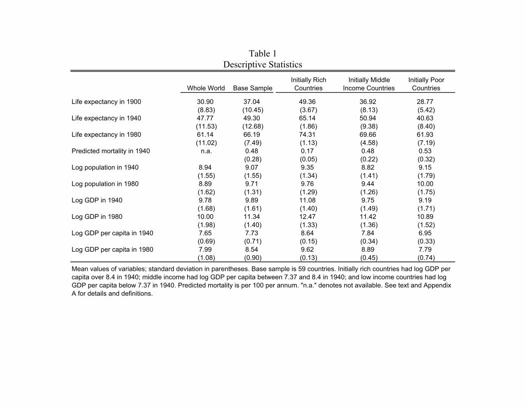
Whole World Base SampleInitially Rich Countries

Initially Middle Income Countries

Initially Poor Countries

Life expectancy in 1900 30.90 37.04 49.36 36.92 28.77(8.83) (10.45) (3.67) (8.13) (5.42)

Life expectancy in 1940 47.77 49.30 65.14 50.94 40.63(11.53) (12.68) (1.86) (9.38) (8.40)

Life expectancy in 1980 61.14 66.19 74.31 69.66 61.93(11.02) (7.49) (1.13) (4.58) (7.19)

Predicted mortality in 1940 n.a. 0.48 0.17 0.48 0.53(0.28) (0.05) (0.22) (0.32)

Log population in 1940 8.94 9.07 9.35 8.82 9.15(1.55) (1.55) (1.34) (1.41) (1.79)

Log population in 1980 8.89 9.71 9.76 9.44 10.00(1.62) (1.31) (1.29) (1.26) (1.75)

Log GDP in 1940 9.78 9.89 11.08 9.75 9.19(1.68) (1.61) (1.40) (1.49) (1.71)

Log GDP in 1980 10.00 11.34 12.47 11.42 10.89(1.98) (1.40) (1.33) (1.36) (1.52)

Log GDP per capita in 1940 7.65 7.73 8.64 7.84 6.95(0.69) (0.71) (0.15) (0.34) (0.33)

Log GDP per capita in 1980 7.99 8.54 9.62 8.89 7.79(1.08) (0.90) (0.13) (0.45) (0.74)

Table 1Descriptive Statistics

Mean values of variables; standard deviation in parentheses. Base sample is 59 countries. Initially rich countries had log GDP per capita over 8.4 in 1940; middle income had log GDP per capita between 7.37 and 8.4 in 1940; and low income countries had log GDP per capita below 7.37 in 1940. Predicted mortality is per 100 per annum. "n.a." denotes not available. See text and Appendix A for details and definitions.

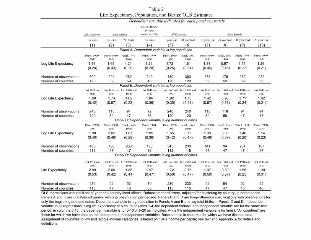
All Countries

Low & Middle Income

Countries Only

No leads No leads No leads No leads 10 year lead 20 year lead 10 year lead 20 year lead 10 year lead 20 year lead

(1) (2) (3) (4) (5) (6) (7) (8) (9) (10)

Panel, 1960-2000

Panel, 1960-2000

Panel, 1940-1980

Panel, 1940-1980

Panel, 1960-1990

Panel, 1960-1980

Panel, 1960-1990

Panel, 1960-1980

Panel, 1940-1980

Panel, 1940-1980

Log Life Expectancy 1.46 1.69 1.21 1.24 1.72 1.61 1.34 0.97 1.33 1.26(0.29) (0.43) (0.20) (0.28) (0.26) (0.34) (0.46) (0.46) (0.22) (0.21)

Number of observations 600 294 282 249 480 360 235 176 282 282Number of countries 120 59 59 48 120 120 59 59 59 59

Just 1960 and 2000

Just 1960 and 2000

Just 1940 and 1980

Just 1940 and 1980

Just 1960 and 1990

Just 1960 and 1980

Just 1960 and 1990

Just 1960 and 1980

Just 1940 and 1980

Just 1940 and 1980

Log Life Expectancy 1.60 1.74 1.62 1.86 1.92 1.70 1.42 0.98 1.71 1.62(0.42) (0.57) (0.22) (0.36) (0.35) (0.41) (0.57) (0.58) (0.24) (0.21)

Number of observations 240 118 94 72 240 240 118 118 94 94Number of countries 120 59 47 36 120 120 59 59 47 47

Panel, 1960-1990

Panel, 1960-1990

Panel, 1940-1980

Panel, 1940-1980

Panel, 1960-1990

Panel, 1960-1980

Panel, 1960-1990

Panel, 1960-1980

Panel, 1930-1970

Panel, 1930-1970

Log Life Expectancy 1.90 2.02 1.87 1.85 1.65 0.75 1.39 0.30 1.46 1.14(0.40) (0.46) (0.28) (0.36) (0.42) (0.47) (0.49) (0.57) (0.20) (0.23)

Number of observations 460 188 233 198 345 230 141 94 234 187Number of countries 115 47 47 36 115 115 47 47 47 47

Just 1960 and 1990

Just 1960 and 1990

Just 1940 and 1980

Just 1940 and 1980

Just 1960 and 1980

Just 1960 and 1970

Just 1960 and 1980

Just 1960 and 1970

Just 1940 and 1980

Just 1940 and 1970

Life Expectancy 2.09 2.00 1.88 1.97 1.72 0.75 1.37 0.30 1.55 1.30(0.53) (0.42) (0.41) (0.47) (0.50) (0.47) (0.59) (0.57) (0.25) (0.31)

Number of observations 230 94 92 70 230 230 94 94 92 92Number of countries 115 47 46 35 115 115 47 47 46 46

Table 2

Base Sample

Panel D: Dependent variable is log number of births

Life Expectancy, Population, and Births: OLS Estimates

Panel C: Dependent variable is log number of births

Panel A: Dependent variable is log population

Panel B: Dependent variable is log population

Dependent variable indicated for each panel separately

All Countries

OLS regressions with a full set of year and country fixed effects. Robust standard errors, adjusted for clustering by country, in parentheses. Panels A and C are unbalanced panels with one observation per decade. Panels B and D are long-difference specifications with observations for only the beginning and end dates. Dependent variable is log population in Panels A and B and log total births in Panels C and D. Independent variable in all regressions is log life expectancy at birth. In columns 1-4, the dependent variable and independent variable are for the same time period; in columns 5-10, the dependent variable is for t+10 or t+20 as indicated, while the independent variable is for time t. "All countries" are those for which we have data on the dependent and independent variables. Base sample is countries for which we have disease data. Assignment of countries to low and middle income categories is based on 1940 income per capita; see text and Appendix A for details and definitions.

Base Sample

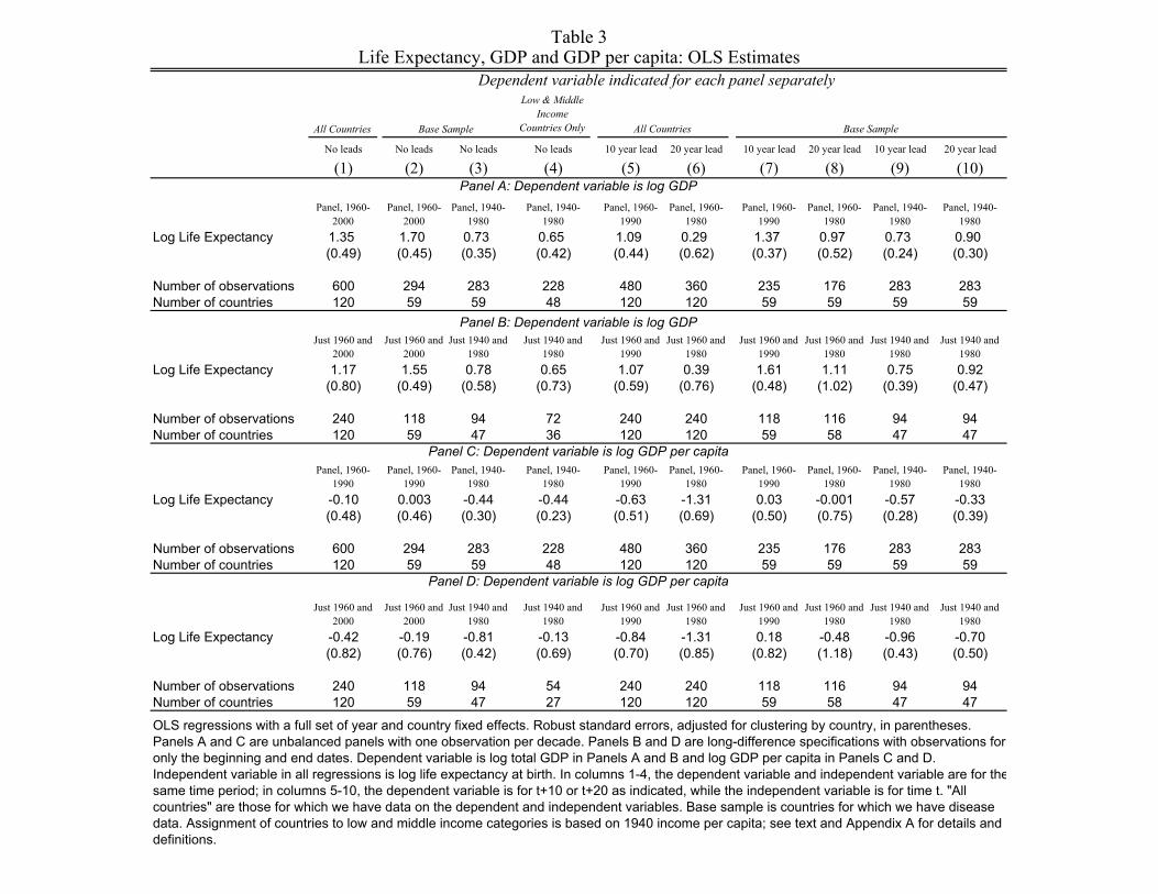
All Countries

Low & Middle Income

Countries Only

No leads No leads No leads No leads 10 year lead 20 year lead 10 year lead 20 year lead 10 year lead 20 year lead

(1) (2) (3) (4) (5) (6) (7) (8) (9) (10)

Panel, 1960-2000

Panel, 1960-2000

Panel, 1940-1980

Panel, 1940-1980

Panel, 1960-1990

Panel, 1960-1980

Panel, 1960-1990

Panel, 1960-1980

Panel, 1940-1980

Panel, 1940-1980

Log Life Expectancy 1.35 1.70 0.73 0.65 1.09 0.29 1.37 0.97 0.73 0.90(0.49) (0.45) (0.35) (0.42) (0.44) (0.62) (0.37) (0.52) (0.24) (0.30)

Number of observations 600 294 283 228 480 360 235 176 283 283Number of countries 120 59 59 48 120 120 59 59 59 59

Just 1960 and 2000

Just 1960 and 2000

Just 1940 and 1980

Just 1940 and 1980

Just 1960 and 1990

Just 1960 and 1980

Just 1960 and 1990

Just 1960 and 1980

Just 1940 and 1980

Just 1940 and 1980

Log Life Expectancy 1.17 1.55 0.78 0.65 1.07 0.39 1.61 1.11 0.75 0.92(0.80) (0.49) (0.58) (0.73) (0.59) (0.76) (0.48) (1.02) (0.39) (0.47)

Number of observations 240 118 94 72 240 240 118 116 94 94Number of countries 120 59 47 36 120 120 59 58 47 47

Panel, 1960-1990

Panel, 1960-1990

Panel, 1940-1980

Panel, 1940-1980

Panel, 1960-1990

Panel, 1960-1980

Panel, 1960-1990

Panel, 1960-1980

Panel, 1940-1980

Panel, 1940-1980

Log Life Expectancy -0.10 0.003 -0.44 -0.44 -0.63 -1.31 0.03 -0.001 -0.57 -0.33(0.48) (0.46) (0.30) (0.23) (0.51) (0.69) (0.50) (0.75) (0.28) (0.39)

Number of observations 600 294 283 228 480 360 235 176 283 283Number of countries 120 59 59 48 120 120 59 59 59 59

Just 1960 and 2000

Just 1960 and 2000

Just 1940 and 1980

Just 1940 and 1980

Just 1960 and 1990

Just 1960 and 1980

Just 1960 and 1990

Just 1960 and 1980

Just 1940 and 1980

Just 1940 and 1980

Log Life Expectancy -0.42 -0.19 -0.81 -0.13 -0.84 -1.31 0.18 -0.48 -0.96 -0.70(0.82) (0.76) (0.42) (0.69) (0.70) (0.85) (0.82) (1.18) (0.43) (0.50)

Number of observations 240 118 94 54 240 240 118 116 94 94Number of countries 120 59 47 27 120 120 59 58 47 47

Table 3

Panel C: Dependent variable is log GDP per capita

Panel A: Dependent variable is log GDP

Panel B: Dependent variable is log GDP

Dependent variable indicated for each panel separately

All Countries

Life Expectancy, GDP and GDP per capita: OLS Estimates

OLS regressions with a full set of year and country fixed effects. Robust standard errors, adjusted for clustering by country, in parentheses. Panels A and C are unbalanced panels with one observation per decade. Panels B and D are long-difference specifications with observations for only the beginning and end dates. Dependent variable is log total GDP in Panels A and B and log GDP per capita in Panels C and D. Independent variable in all regressions is log life expectancy at birth. In columns 1-4, the dependent variable and independent variable are for thesame time period; in columns 5-10, the dependent variable is for t+10 or t+20 as indicated, while the independent variable is for time t. "All countries" are those for which we have data on the dependent and independent variables. Base sample is countries for which we have disease data. Assignment of countries to low and middle income categories is based on 1940 income per capita; see text and Appendix A for details and definitions.

Panel D: Dependent variable is log GDP per capita

Base Sample Base Sample

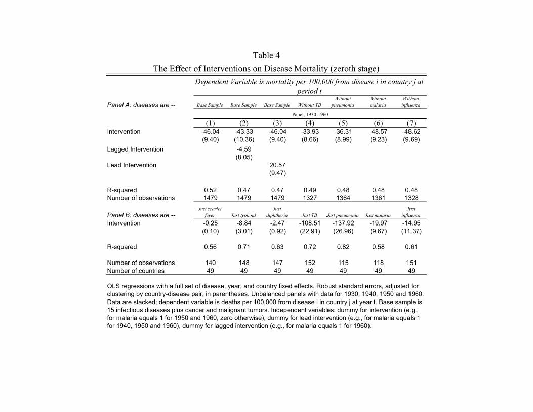
Panel A: diseases are -- Base Sample Base Sample Base Sample Without TBWithout

pneumoniaWithout malaria

Without influenza

(1) (2) (3) (4) (5) (6) (7)Intervention -46.04 -43.33 -46.04 -33.93 -36.31 -48.57 -48.62

(9.40) (10.36) (9.40) (8.66) (8.99) (9.23) (9.69)Lagged Intervention -4.59

(8.05)Lead Intervention 20.57

(9.47)

R-squared 0.52 0.47 0.47 0.49 0.48 0.48 0.48Number of observations 1479 1479 1479 1327 1364 1361 1328

Panel B: diseases are --Just scarlet

fever Just typhoidJust

diphtheria Just TB Just pneumonia Just malariaJust

influenzaIntervention -0.25 -8.84 -2.47 -108.51 -137.92 -19.97 -14.95

(0.10) (3.01) (0.92) (22.91) (26.96) (9.67) (11.37)

R-squared 0.56 0.71 0.63 0.72 0.82 0.58 0.61

Number of observations 140 148 147 152 115 118 151Number of countries 49 49 49 49 49 49 49

OLS regressions with a full set of disease, year, and country fixed effects. Robust standard errors, adjusted for clustering by country-disease pair, in parentheses. Unbalanced panels with data for 1930, 1940, 1950 and 1960. Data are stacked; dependent variable is deaths per 100,000 from disease i in country j at year t. Base sample is 15 infectious diseases plus cancer and malignant tumors. Independent variables: dummy for intervention (e.g., for malaria equals 1 for 1950 and 1960, zero otherwise), dummy for lead intervention (e.g., for malaria equals 1 for 1940, 1950 and 1960), dummy for lagged intervention (e.g., for malaria equals 1 for 1960).

Panel, 1930-1960

Table 4The Effect of Interventions on Disease Mortality (zeroth stage)

Dependent Variable is mortality per 100,000 from disease i in country j at period t

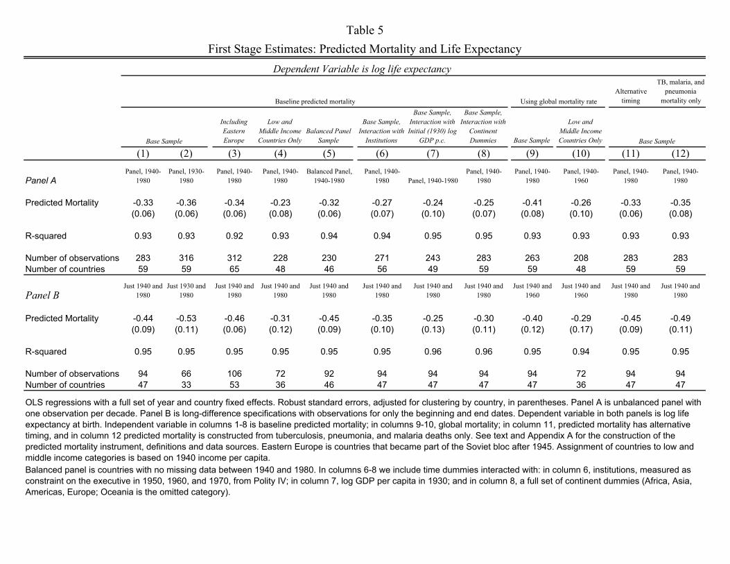
Alternative timing

TB, malaria, and pneumonia

mortality only

Including Eastern Europe

Low and Middle Income Countries Only

Balanced Panel Sample

Base Sample, Interaction with

Institutions

Base Sample, Interaction with Initial (1930) log

GDP p.c.

Base Sample, Interaction with

Continent Dummies Base Sample

Low and Middle Income Countries Only

(1) (2) (3) (4) (5) (6) (7) (8) (9) (10) (11) (12)

Panel APanel, 1940-

1980Panel, 1930-

1980Panel, 1940-

1980Panel, 1940-

1980Balanced Panel,

1940-1980Panel, 1940-

1980 Panel, 1940-1980Panel, 1940-

1980Panel, 1940-

1980Panel, 1940-

1960Panel, 1940-

1980Panel, 1940-

1980

Predicted Mortality -0.33 -0.36 -0.34 -0.23 -0.32 -0.27 -0.24 -0.25 -0.41 -0.26 -0.33 -0.35(0.06) (0.06) (0.06) (0.08) (0.06) (0.07) (0.10) (0.07) (0.08) (0.10) (0.06) (0.08)

R-squared 0.93 0.93 0.92 0.93 0.94 0.94 0.95 0.95 0.93 0.93 0.93 0.93

Number of observations 283 316 312 228 230 271 243 283 263 208 283 283Number of countries 59 59 65 48 46 56 49 59 59 48 59 59

Panel BJust 1940 and

1980Just 1930 and

1980Just 1940 and

1980Just 1940 and

1980Just 1940 and

1980Just 1940 and

1980Just 1940 and

1980Just 1940 and

1980Just 1940 and

1960Just 1940 and

1960Just 1940 and

1980Just 1940 and

1980

Predicted Mortality -0.44 -0.53 -0.46 -0.31 -0.45 -0.35 -0.25 -0.30 -0.40 -0.29 -0.45 -0.49(0.09) (0.11) (0.06) (0.12) (0.09) (0.10) (0.13) (0.11) (0.12) (0.17) (0.09) (0.11)

R-squared 0.95 0.95 0.95 0.95 0.95 0.95 0.96 0.96 0.95 0.94 0.95 0.95

Number of observations 94 66 106 72 92 94 94 94 94 72 94 94Number of countries 47 33 53 36 46 47 47 47 47 36 47 47

Balanced panel is countries with no missing data between 1940 and 1980. In columns 6-8 we include time dummies interacted with: in column 6, institutions, measured as constraint on the executive in 1950, 1960, and 1970, from Polity IV; in column 7, log GDP per capita in 1930; and in column 8, a full set of continent dummies (Africa, Asia, Americas, Europe; Oceania is the omitted category).

Table 5

OLS regressions with a full set of year and country fixed effects. Robust standard errors, adjusted for clustering by country, in parentheses. Panel A is unbalanced panel with one observation per decade. Panel B is long-difference specifications with observations for only the beginning and end dates. Dependent variable in both panels is log life expectancy at birth. Independent variable in columns 1-8 is baseline predicted mortality; in columns 9-10, global mortality; in column 11, predicted mortality has alternative timing, and in column 12 predicted mortality is constructed from tuberculosis, pneumonia, and malaria deaths only. See text and Appendix A for the construction of the predicted mortality instrument, definitions and data sources. Eastern Europe is countries that became part of the Soviet bloc after 1945. Assignment of countries to low and middle income categories is based on 1940 income per capita.

Base Sample

Dependent Variable is log life expectancy

Using global mortality rate

First Stage Estimates: Predicted Mortality and Life Expectancy

Base Sample

Baseline predicted mortality

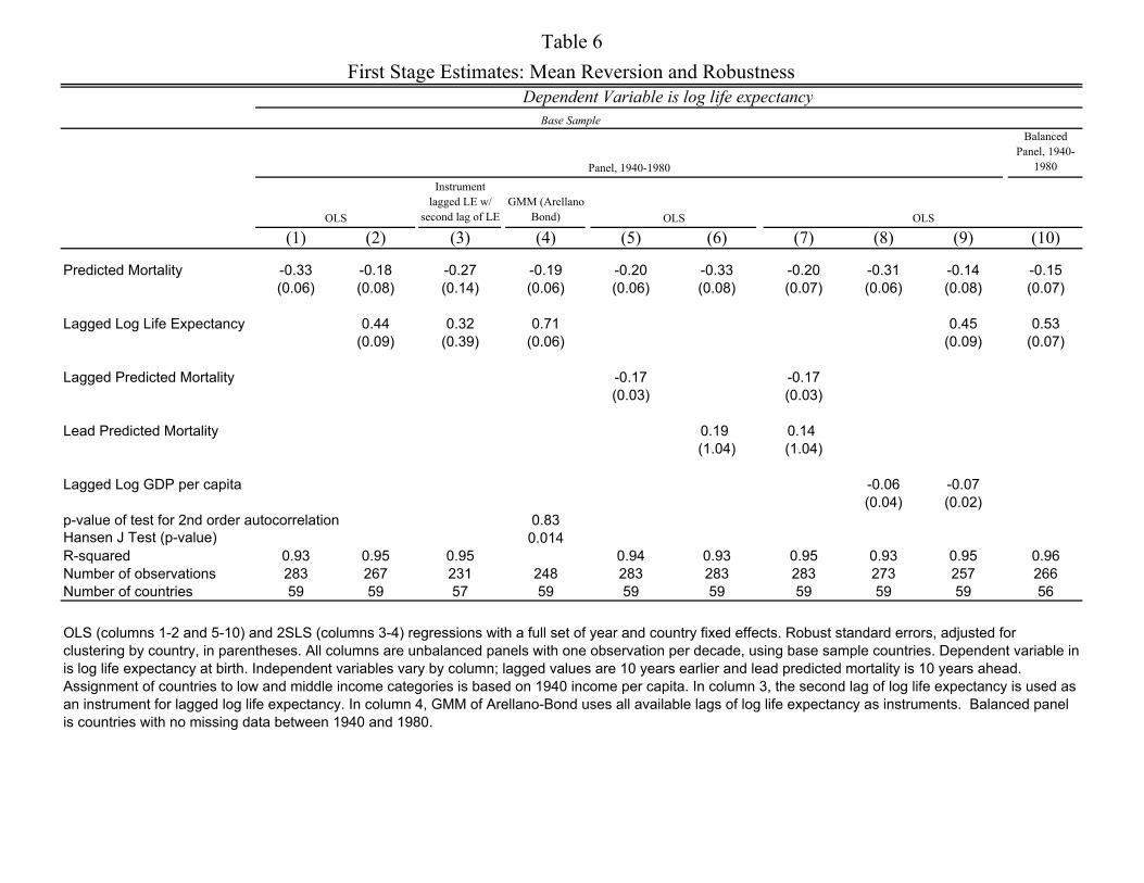
Balanced Panel, 1940-

1980

Instrument lagged LE w/

second lag of LEGMM (Arellano

Bond)

(1) (2) (3) (4) (5) (6) (7) (8) (9) (10)

Predicted Mortality -0.33 -0.18 -0.27 -0.19 -0.20 -0.33 -0.20 -0.31 -0.14 -0.15(0.06) (0.08) (0.14) (0.06) (0.06) (0.08) (0.07) (0.06) (0.08) (0.07)

Lagged Log Life Expectancy 0.44 0.32 0.71 0.45 0.53(0.09) (0.39) (0.06) (0.09) (0.07)

Lagged Predicted Mortality -0.17 -0.17(0.03) (0.03)

Lead Predicted Mortality 0.19 0.14(1.04) (1.04)

Lagged Log GDP per capita -0.06 -0.07(0.04) (0.02)

p-value of test for 2nd order autocorrelation 0.83Hansen J Test (p-value) 0.014R-squared 0.93 0.95 0.95 0.94 0.93 0.95 0.93 0.95 0.96Number of observations 283 267 231 248 283 283 283 273 257 266Number of countries 59 59 57 59 59 59 59 59 59 56

Panel, 1940-1980

OLS (columns 1-2 and 5-10) and 2SLS (columns 3-4) regressions with a full set of year and country fixed effects. Robust standard errors, adjusted for clustering by country, in parentheses. All columns are unbalanced panels with one observation per decade, using base sample countries. Dependent variable in is log life expectancy at birth. Independent variables vary by column; lagged values are 10 years earlier and lead predicted mortality is 10 years ahead. Assignment of countries to low and middle income categories is based on 1940 income per capita. In column 3, the second lag of log life expectancy is used as an instrument for lagged log life expectancy. In column 4, GMM of Arellano-Bond uses all available lags of log life expectancy as instruments. Balanced panel is countries with no missing data between 1940 and 1980.

Base Sample

Table 6First Stage Estimates: Mean Reversion and Robustness

Dependent Variable is log life expectancy

OLS OLS OLS

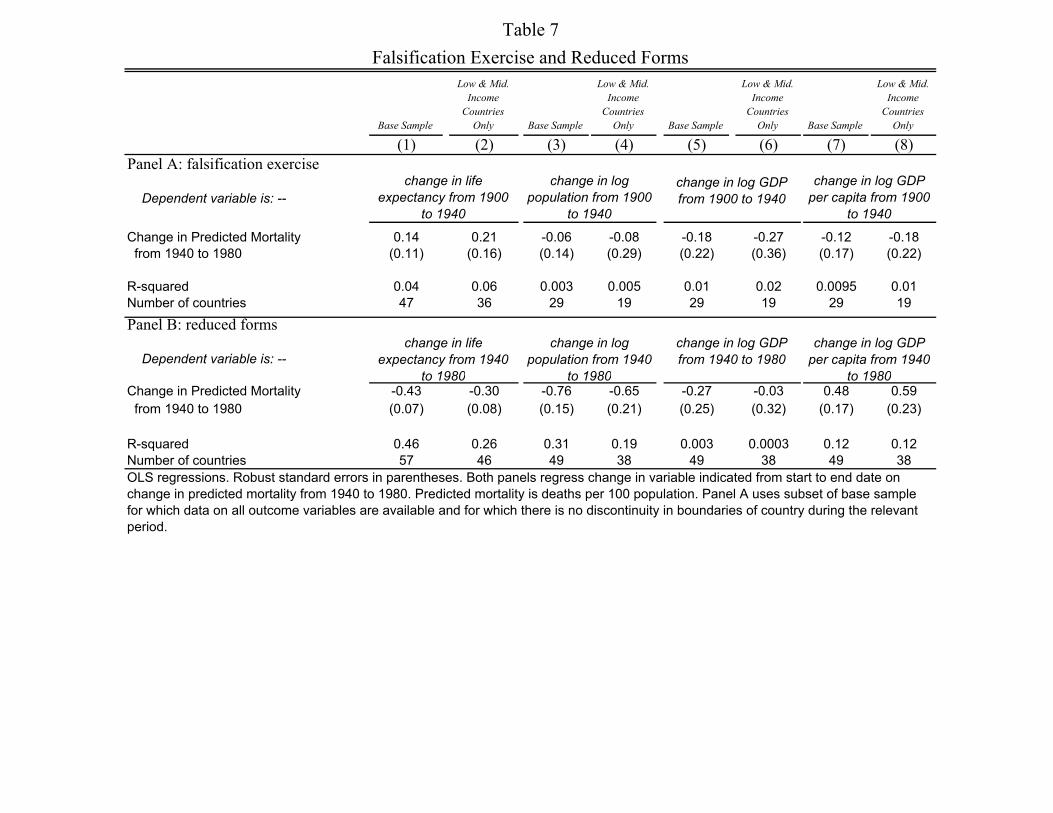
Base Sample

Low & Mid. Income

Countries Only Base Sample

Low & Mid. Income

Countries Only Base Sample

Low & Mid. Income

Countries Only Base Sample

Low & Mid. Income

Countries Only

(1) (2) (3) (4) (5) (6) (7) (8)Panel A: falsification exercise

Dependent variable is: --

Change in Predicted Mortality 0.14 0.21 -0.06 -0.08 -0.18 -0.27 -0.12 -0.18 from 1940 to 1980 (0.11) (0.16) (0.14) (0.29) (0.22) (0.36) (0.17) (0.22)

R-squared 0.04 0.06 0.003 0.005 0.01 0.02 0.0095 0.01Number of countries 47 36 29 19 29 19 29 19

Panel B: reduced forms

Dependent variable is: --

Change in Predicted Mortality -0.43 -0.30 -0.76 -0.65 -0.27 -0.03 0.48 0.59 from 1940 to 1980 (0.07) (0.08) (0.15) (0.21) (0.25) (0.32) (0.17) (0.23)

R-squared 0.46 0.26 0.31 0.19 0.003 0.0003 0.12 0.12Number of countries 57 46 49 38 49 38 49 38

change in log GDP per capita from 1900

to 1940

Falsification Exercise and Reduced FormsTable 7

change in log population from 1900

to 1940

change in log GDP from 1900 to 1940

change in life expectancy from 1900

to 1940

change in life expectancy from 1940

to 1980

OLS regressions. Robust standard errors in parentheses. Both panels regress change in variable indicated from start to end date on change in predicted mortality from 1940 to 1980. Predicted mortality is deaths per 100 population. Panel A uses subset of base sample for which data on all outcome variables are available and for which there is no discontinuity in boundaries of country during the relevant period.

change in log population from 1940

to 1980

change in log GDP from 1940 to 1980

change in log GDP per capita from 1940

to 1980

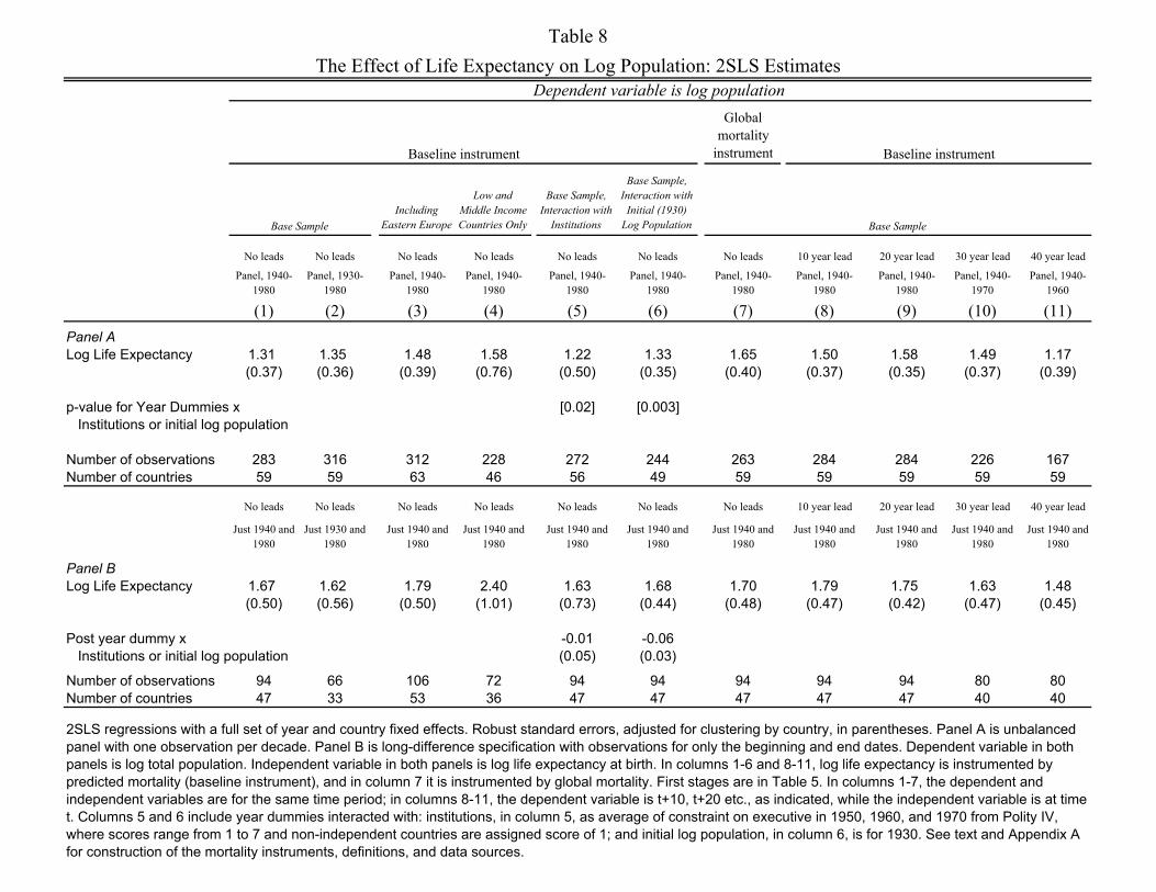
Global

mortality instrument

Including Eastern Europe

Low and Middle Income Countries Only

Base Sample, Interaction with

Institutions

Base Sample, Interaction with

Initial (1930) Log Population

No leads No leads No leads No leads No leads No leads No leads 10 year lead 20 year lead 30 year lead 40 year lead

Panel, 1940-1980

Panel, 1930-1980

Panel, 1940-1980

Panel, 1940-1980

Panel, 1940-1980

Panel, 1940-1980

Panel, 1940-1980

Panel, 1940-1980

Panel, 1940-1980

Panel, 1940-1970

Panel, 1940-1960

(1) (2) (3) (4) (5) (6) (7) (8) (9) (10) (11)Panel ALog Life Expectancy 1.31 1.35 1.48 1.58 1.22 1.33 1.65 1.50 1.58 1.49 1.17

(0.37) (0.36) (0.39) (0.76) (0.50) (0.35) (0.40) (0.37) (0.35) (0.37) (0.39)

p-value for Year Dummies x [0.02] [0.003] Institutions or initial log population

Number of observations 283 316 312 228 272 244 263 284 284 226 167Number of countries 59 59 63 46 56 49 59 59 59 59 59

No leads No leads No leads No leads No leads No leads No leads 10 year lead 20 year lead 30 year lead 40 year lead

Just 1940 and 1980

Just 1930 and 1980

Just 1940 and 1980

Just 1940 and 1980

Just 1940 and 1980

Just 1940 and 1980

Just 1940 and 1980

Just 1940 and 1980

Just 1940 and 1980

Just 1940 and 1980

Just 1940 and 1980

Panel BLog Life Expectancy 1.67 1.62 1.79 2.40 1.63 1.68 1.70 1.79 1.75 1.63 1.48

(0.50) (0.56) (0.50) (1.01) (0.73) (0.44) (0.48) (0.47) (0.42) (0.47) (0.45)

Post year dummy x -0.01 -0.06 Institutions or initial log population (0.05) (0.03)

Number of observations 94 66 106 72 94 94 94 94 94 80 80Number of countries 47 33 53 36 47 47 47 47 47 40 40

2SLS regressions with a full set of year and country fixed effects. Robust standard errors, adjusted for clustering by country, in parentheses. Panel A is unbalanced panel with one observation per decade. Panel B is long-difference specification with observations for only the beginning and end dates. Dependent variable in both panels is log total population. Independent variable in both panels is log life expectancy at birth. In columns 1-6 and 8-11, log life expectancy is instrumented by predicted mortality (baseline instrument), and in column 7 it is instrumented by global mortality. First stages are in Table 5. In columns 1-7, the dependent and independent variables are for the same time period; in columns 8-11, the dependent variable is t+10, t+20 etc., as indicated, while the independent variable is at time t. Columns 5 and 6 include year dummies interacted with: institutions, in column 5, as average of constraint on executive in 1950, 1960, and 1970 from Polity IV, where scores range from 1 to 7 and non-independent countries are assigned score of 1; and initial log population, in column 6, is for 1930. See text and Appendix A for construction of the mortality instruments, definitions, and data sources.

Baseline instrument

Table 8

Base Sample

The Effect of Life Expectancy on Log Population: 2SLS EstimatesDependent variable is log population

Base Sample

Baseline instrument

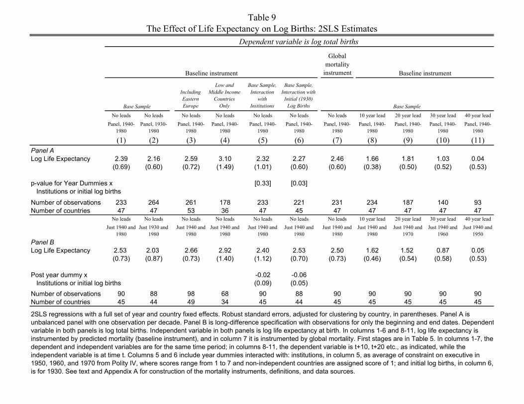
Global mortality

instrument

Including Eastern Europe

Low and Middle Income

Countries Only

Base Sample, Interaction

with Institutions

Base Sample, Interaction with

Initial (1930) Log Births

No leads No leads No leads No leads No leads No leads No leads 10 year lead 20 year lead 30 year lead 40 year leadPanel, 1940-

1980Panel, 1930-

1980Panel, 1940-

1980Panel, 1940-

1980Panel, 1940-

1980Panel, 1940-

1980Panel, 1940-

1980Panel, 1940-

1980Panel, 1940-

1980Panel, 1940-

1980Panel, 1940-

1980

(1) (2) (3) (4) (5) (6) (7) (8) (9) (10) (11)Panel ALog Life Expectancy 2.39 2.16 2.59 3.10 2.32 2.27 2.46 1.66 1.81 1.03 0.04

(0.69) (0.60) (0.72) (1.49) (1.01) (0.60) (0.60) (0.38) (0.50) (0.52) (0.53)

p-value for Year Dummies x [0.33] [0.03] Institutions or initial log births

Number of observations 233 264 261 178 233 221 231 234 187 140 93Number of countries 47 47 53 36 47 45 47 47 47 47 47

No leads No leads No leads No leads No leads No leads No leads 10 year lead 20 year lead 30 year lead 40 year leadJust 1940 and

1980Just 1930 and

1980Just 1940 and

1980Just 1940 and

1980Just 1940 and

1980Just 1940 and

1980Just 1940 and

1980Just 1940 and

1980Just 1940 and

1970Just 1940 and

1960Just 1940 and

1950Panel BLog Life Expectancy 2.53 2.03 2.66 2.92 2.40 2.53 2.50 1.62 1.52 0.87 0.05

(0.73) (0.87) (0.73) (1.40) (1.12) (0.70) (0.73) (0.46) (0.54) (0.58) (0.53)

Post year dummy x -0.02 -0.06 Institutions or initial log births (0.09) (0.05)Number of observations 90 88 98 68 90 88 90 90 90 90 90Number of countries 45 44 49 34 45 44 45 45 45 45 45

2SLS regressions with a full set of year and country fixed effects. Robust standard errors, adjusted for clustering by country, in parentheses. Panel A is unbalanced panel with one observation per decade. Panel B is long-difference specification with observations for only the beginning and end dates. Dependentvariable in both panels is log total births. Independent variable in both panels is log life expectancy at birth. In columns 1-6 and 8-11, log life expectancy is instrumented by predicted mortality (baseline instrument), and in column 7 it is instrumented by global mortality. First stages are in Table 5. In columns 1-7, the dependent and independent variables are for the same time period; in columns 8-11, the dependent variable is t+10, t+20 etc., as indicated, while the independent variable is at time t. Columns 5 and 6 include year dummies interacted with: institutions, in column 5, as average of constraint on executive in 1950, 1960, and 1970 from Polity IV, where scores range from 1 to 7 and non-independent countries are assigned score of 1; and initial log births, in column 6, is for 1930. See text and Appendix A for construction of the mortality instruments, definitions, and data sources.

Base Sample

Table 9The Effect of Life Expectancy on Log Births: 2SLS Estimates

Dependent variable is log total births

Baseline instrument

Base Sample

Baseline instrument

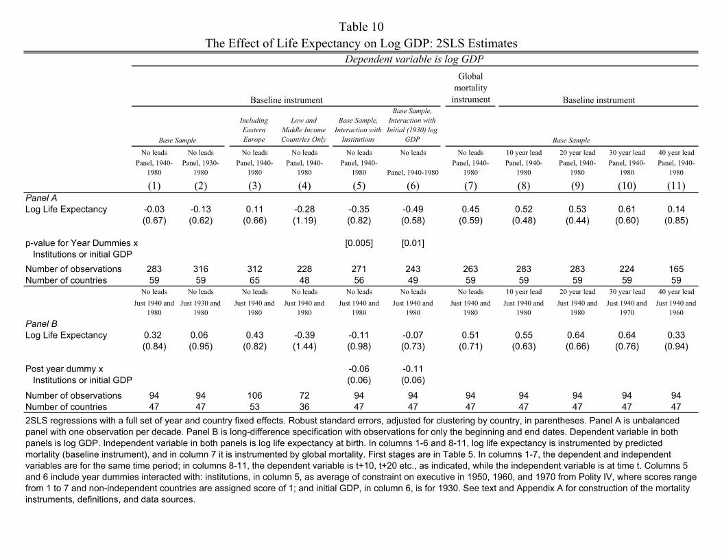
Global

mortality instrument

Including Eastern Europe

Low and Middle Income Countries Only

Base Sample, Interaction with

Institutions

Base Sample, Interaction with Initial (1930) log

GDP

No leads No leads No leads No leads No leads No leads No leads 10 year lead 20 year lead 30 year lead 40 year leadPanel, 1940-

1980Panel, 1930-

1980Panel, 1940-

1980Panel, 1940-

1980Panel, 1940-

1980 Panel, 1940-1980Panel, 1940-

1980Panel, 1940-

1980Panel, 1940-

1980Panel, 1940-

1980Panel, 1940-

1980

(1) (2) (3) (4) (5) (6) (7) (8) (9) (10) (11)Panel ALog Life Expectancy -0.03 -0.13 0.11 -0.28 -0.35 -0.49 0.45 0.52 0.53 0.61 0.14

(0.67) (0.62) (0.66) (1.19) (0.82) (0.58) (0.59) (0.48) (0.44) (0.60) (0.85)

p-value for Year Dummies x [0.005] [0.01] Institutions or initial GDPNumber of observations 283 316 312 228 271 243 263 283 283 224 165Number of countries 59 59 65 48 56 49 59 59 59 59 59

No leads No leads No leads No leads No leads No leads No leads 10 year lead 20 year lead 30 year lead 40 year leadJust 1940 and

1980Just 1930 and

1980Just 1940 and

1980Just 1940 and

1980Just 1940 and

1980Just 1940 and

1980Just 1940 and

1980Just 1940 and

1980Just 1940 and

1980Just 1940 and

1970Just 1940 and

1960Panel BLog Life Expectancy 0.32 0.06 0.43 -0.39 -0.11 -0.07 0.51 0.55 0.64 0.64 0.33

(0.84) (0.95) (0.82) (1.44) (0.98) (0.73) (0.71) (0.63) (0.66) (0.76) (0.94)

Post year dummy x -0.06 -0.11 Institutions or initial GDP (0.06) (0.06)

Number of observations 94 94 106 72 94 94 94 94 94 94 94Number of countries 47 47 53 36 47 47 47 47 47 47 472SLS regressions with a full set of year and country fixed effects. Robust standard errors, adjusted for clustering by country, in parentheses. Panel A is unbalanced panel with one observation per decade. Panel B is long-difference specification with observations for only the beginning and end dates. Dependent variable in both panels is log GDP. Independent variable in both panels is log life expectancy at birth. In columns 1-6 and 8-11, log life expectancy is instrumented by predicted mortality (baseline instrument), and in column 7 it is instrumented by global mortality. First stages are in Table 5. In columns 1-7, the dependent and independent variables are for the same time period; in columns 8-11, the dependent variable is t+10, t+20 etc., as indicated, while the independent variable is at time t. Columns 5 and 6 include year dummies interacted with: institutions, in column 5, as average of constraint on executive in 1950, 1960, and 1970 from Polity IV, where scores range from 1 to 7 and non-independent countries are assigned score of 1; and initial GDP, in column 6, is for 1930. See text and Appendix A for construction of the mortality instruments, definitions, and data sources.

Base Sample

Table 10The Effect of Life Expectancy on Log GDP: 2SLS Estimates

Dependent variable is log GDP

Baseline instrument

Base Sample

Baseline instrument

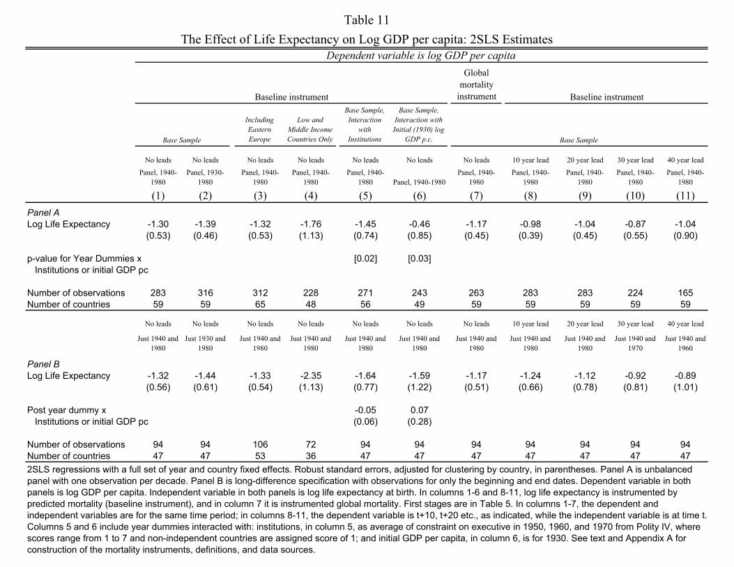
Global

mortality instrument

Including Eastern Europe

Low and Middle Income Countries Only

Base Sample, Interaction

with Institutions

Base Sample, Interaction with Initial (1930) log

GDP p.c.

No leads No leads No leads No leads No leads No leads No leads 10 year lead 20 year lead 30 year lead 40 year lead

Panel, 1940-1980

Panel, 1930-1980

Panel, 1940-1980

Panel, 1940-1980

Panel, 1940-1980 Panel, 1940-1980

Panel, 1940-1980

Panel, 1940-1980

Panel, 1940-1980

Panel, 1940-1980

Panel, 1940-1980

(1) (2) (3) (4) (5) (6) (7) (8) (9) (10) (11)Panel ALog Life Expectancy -1.30 -1.39 -1.32 -1.76 -1.45 -0.46 -1.17 -0.98 -1.04 -0.87 -1.04

(0.53) (0.46) (0.53) (1.13) (0.74) (0.85) (0.45) (0.39) (0.45) (0.55) (0.90)

p-value for Year Dummies x [0.02] [0.03] Institutions or initial GDP pc

Number of observations 283 316 312 228 271 243 263 283 283 224 165Number of countries 59 59 65 48 56 49 59 59 59 59 59

No leads No leads No leads No leads No leads No leads No leads 10 year lead 20 year lead 30 year lead 40 year lead

Just 1940 and 1980

Just 1930 and 1980

Just 1940 and 1980

Just 1940 and 1980

Just 1940 and 1980

Just 1940 and 1980

Just 1940 and 1980

Just 1940 and 1980

Just 1940 and 1980

Just 1940 and 1970

Just 1940 and 1960

Panel BLog Life Expectancy -1.32 -1.44 -1.33 -2.35 -1.64 -1.59 -1.17 -1.24 -1.12 -0.92 -0.89

(0.56) (0.61) (0.54) (1.13) (0.77) (1.22) (0.51) (0.66) (0.78) (0.81) (1.01)

Post year dummy x -0.05 0.07 Institutions or initial GDP pc (0.06) (0.28)

Number of observations 94 94 106 72 94 94 94 94 94 94 94Number of countries 47 47 53 36 47 47 47 47 47 47 472SLS regressions with a full set of year and country fixed effects. Robust standard errors, adjusted for clustering by country, in parentheses. Panel A is unbalanced panel with one observation per decade. Panel B is long-difference specification with observations for only the beginning and end dates. Dependent variable in both panels is log GDP per capita. Independent variable in both panels is log life expectancy at birth. In columns 1-6 and 8-11, log life expectancy is instrumented by predicted mortality (baseline instrument), and in column 7 it is instrumented global mortality. First stages are in Table 5. In columns 1-7, the dependent and independent variables are for the same time period; in columns 8-11, the dependent variable is t+10, t+20 etc., as indicated, while the independent variable is at time t. Columns 5 and 6 include year dummies interacted with: institutions, in column 5, as average of constraint on executive in 1950, 1960, and 1970 from Polity IV, where scores range from 1 to 7 and non-independent countries are assigned score of 1; and initial GDP per capita, in column 6, is for 1930. See text and Appendix A for construction of the mortality instruments, definitions, and data sources.

Baseline instrument

Table 11

Base Sample

The Effect of Life Expectancy on Log GDP per capita: 2SLS EstimatesDependent variable is log GDP per capita

Base Sample

Baseline instrument

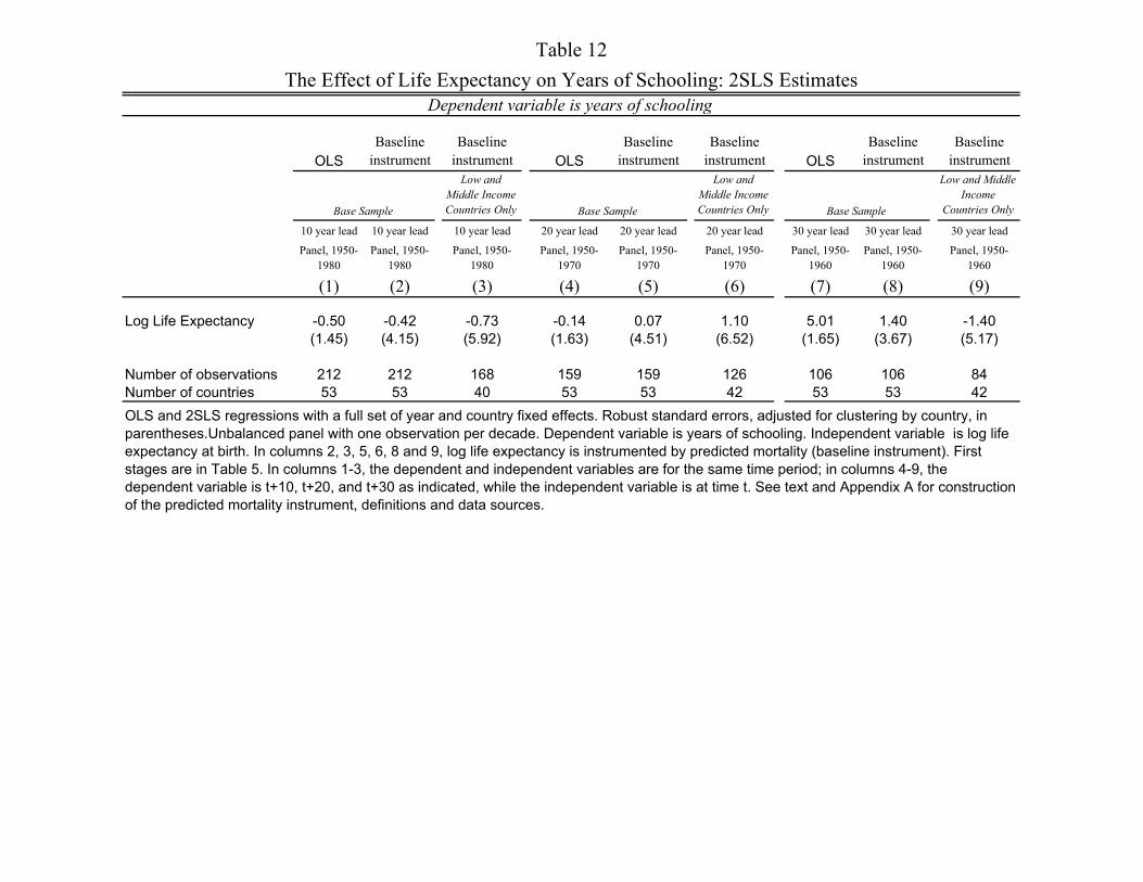
OLSBaseline

instrumentBaseline

instrument OLSBaseline

instrumentBaseline

instrument OLSBaseline

instrumentBaseline

instrumentLow and

Middle Income Countries Only

Low and Middle Income Countries Only

Low and Middle Income

Countries Only

10 year lead 10 year lead 10 year lead 20 year lead 20 year lead 20 year lead 30 year lead 30 year lead 30 year lead

Panel, 1950-1980

Panel, 1950-1980

Panel, 1950-1980

Panel, 1950-1970

Panel, 1950-1970

Panel, 1950-1970

Panel, 1950-1960

Panel, 1950-1960

Panel, 1950-1960

(1) (2) (3) (4) (5) (6) (7) (8) (9) Log Life Expectancy -0.50 -0.42 -0.73 -0.14 0.07 1.10 5.01 1.40 -1.40

(1.45) (4.15) (5.92) (1.63) (4.51) (6.52) (1.65) (3.67) (5.17)

Number of observations 212 212 168 159 159 126 106 106 84Number of countries 53 53 40 53 53 42 53 53 42

Table 12

Base Sample Base Sample

OLS and 2SLS regressions with a full set of year and country fixed effects. Robust standard errors, adjusted for clustering by country, in parentheses.Unbalanced panel with one observation per decade. Dependent variable is years of schooling. Independent variable is log life expectancy at birth. In columns 2, 3, 5, 6, 8 and 9, log life expectancy is instrumented by predicted mortality (baseline instrument). First stages are in Table 5. In columns 1-3, the dependent and independent variables are for the same time period; in columns 4-9, the dependent variable is t+10, t+20, and t+30 as indicated, while the independent variable is at time t. See text and Appendix A for construction of the predicted mortality instrument, definitions and data sources.

Base Sample

Dependent variable is years of schoolingThe Effect of Life Expectancy on Years of Schooling: 2SLS Estimates

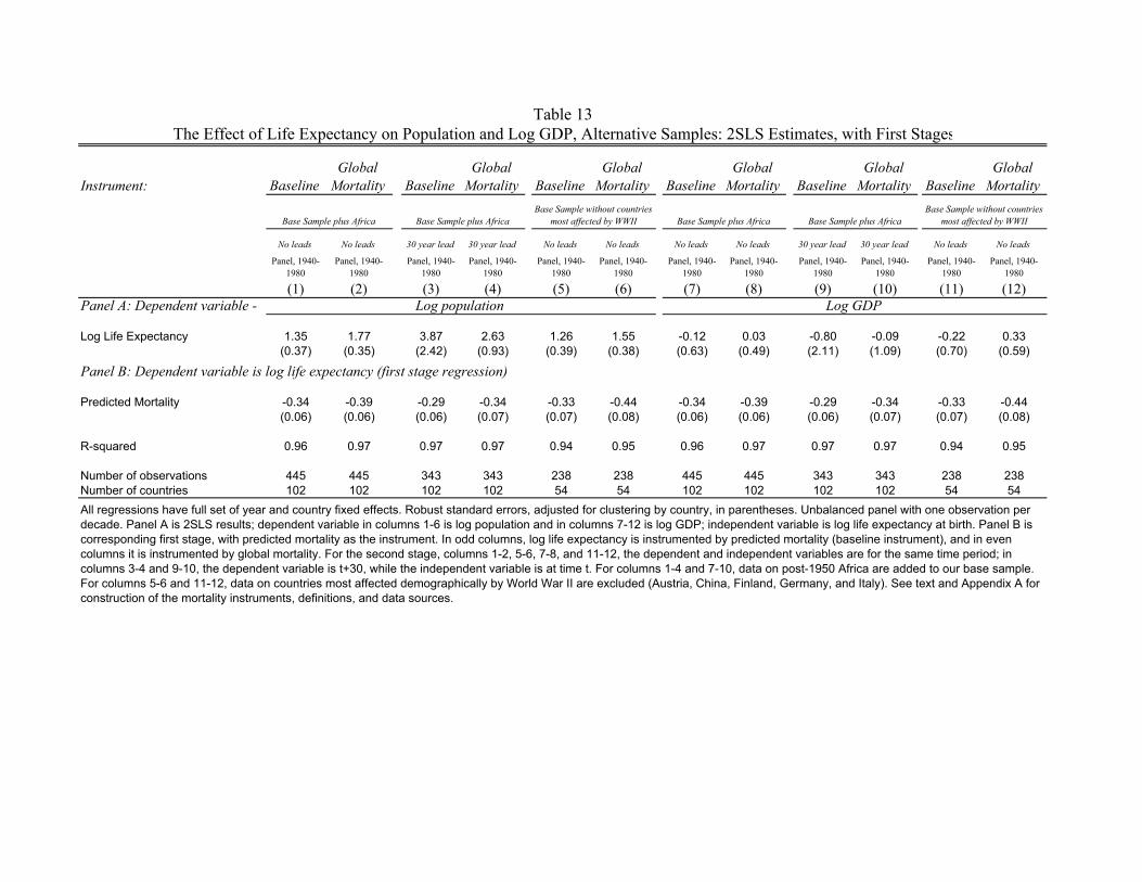
Instrument: BaselineGlobal

Mortality Baseline Global

Mortality Baseline Global

Mortality Baseline Global

Mortality Baseline Global

Mortality Baseline Global

Mortality

No leads No leads 30 year lead 30 year lead No leads No leads No leads No leads 30 year lead 30 year lead No leads No leads

Panel, 1940-1980

Panel, 1940-1980

Panel, 1940-1980

Panel, 1940-1980

Panel, 1940-1980

Panel, 1940-1980

Panel, 1940-1980

Panel, 1940-1980

Panel, 1940-1980

Panel, 1940-1980

Panel, 1940-1980

Panel, 1940-1980

(1) (2) (3) (4) (5) (6) (7) (8) (9) (10) (11) (12)Panel A: Dependent variable -

Log Life Expectancy 1.35 1.77 3.87 2.63 1.26 1.55 -0.12 0.03 -0.80 -0.09 -0.22 0.33(0.37) (0.35) (2.42) (0.93) (0.39) (0.38) (0.63) (0.49) (2.11) (1.09) (0.70) (0.59)

Predicted Mortality -0.34 -0.39 -0.29 -0.34 -0.33 -0.44 -0.34 -0.39 -0.29 -0.34 -0.33 -0.44(0.06) (0.06) (0.06) (0.07) (0.07) (0.08) (0.06) (0.06) (0.06) (0.07) (0.07) (0.08)

R-squared 0.96 0.97 0.97 0.97 0.94 0.95 0.96 0.97 0.97 0.97 0.94 0.95

Number of observations 445 445 343 343 238 238 445 445 343 343 238 238Number of countries 102 102 102 102 54 54 102 102 102 102 54 54

Table 13

Panel B: Dependent variable is log life expectancy (first stage regression)

Base Sample plus AfricaBase Sample without countries

most affected by WWII

The Effect of Life Expectancy on Population and Log GDP, Alternative Samples: 2SLS Estimates, with First Stages

Base Sample plus AfricaBase Sample without countries

most affected by WWIIBase Sample plus Africa

Log GDP

Base Sample plus Africa

All regressions have full set of year and country fixed effects. Robust standard errors, adjusted for clustering by country, in parentheses. Unbalanced panel with one observation per decade. Panel A is 2SLS results; dependent variable in columns 1-6 is log population and in columns 7-12 is log GDP; independent variable is log life expectancy at birth. Panel B is corresponding first stage, with predicted mortality as the instrument. In odd columns, log life expectancy is instrumented by predicted mortality (baseline instrument), and in even columns it is instrumented by global mortality. For the second stage, columns 1-2, 5-6, 7-8, and 11-12, the dependent and independent variables are for the same time period; in columns 3-4 and 9-10, the dependent variable is t+30, while the independent variable is at time t. For columns 1-4 and 7-10, data on post-1950 Africa are added to our base sample. For columns 5-6 and 11-12, data on countries most affected demographically by World War II are excluded (Austria, China, Finland, Germany, and Italy). See text and Appendix A for construction of the mortality instruments, definitions, and data sources.

Log population

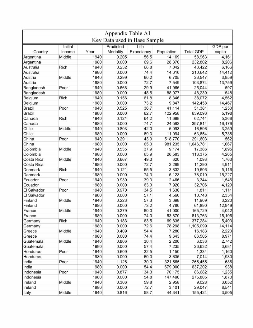
CountryInitial

Income YearPredicted Mortality

Life Expectancy Population Total GDP

GDP per capita

Argentina Middle 1940 0.205 56.5 14,169 58,963 4,161Argentina 1980 0.000 69.6 28,370 232,802 8,206Australia Rich 1940 0.232 66.8 7,042 43,422 6,166Australia 1980 0.000 74.4 14,616 210,642 14,412Austria Middle 1940 0.299 60.2 6,705 26,547 3,959Austria 1980 0.000 72.7 7,549 103,874 13,759Bangladesh Poor 1940 0.668 29.9 41,966 25,044 597Bangladesh 1980 0.000 48.5 88,077 48,239 548Belgium Rich 1940 0.156 61.8 8,346 38,072 4,562Belgium 1980 0.000 73.2 9,847 142,458 14,467Brazil Poor 1940 0.525 36.7 41,114 51,381 1,250Brazil 1980 0.000 62.7 122,958 639,093 5,198Canada Rich 1940 0.121 64.2 11,688 62,744 5,368Canada 1980 0.000 74.7 24,593 397,814 16,176Chile Middle 1940 0.803 42.0 5,093 16,596 3,259Chile 1980 0.000 69.3 11,094 63,654 5,738China Poor 1940 0.291 43.9 518,770 291,603 562China 1980 0.000 65.3 981,235 1,046,781 1,067Colombia Middle 1940 0.535 37.9 9,174 17,386 1,895Colombia 1980 0.000 65.9 26,583 113,375 4,265Costa Rica Middle 1940 0.667 49.3 620 1,093 1,763Costa Rica 1980 0.000 72.7 2,299 11,290 4,911Denmark Rich 1940 0.121 65.5 3,832 19,606 5,116Denmark 1980 0.000 74.3 5,123 78,010 15,227Ecuador Poor 1940 0.930 39.3 2,466 3,344 1,546Ecuador 1980 0.000 63.3 7,920 32,706 4,129El Salvador Poor 1940 0.970 34.5 1,630 1,811 1,111El Salvador 1980 0.000 57.1 4,566 10,748 2,354Finland Middle 1940 0.223 57.3 3,698 11,909 3,220Finland 1980 0.000 73.2 4,780 61,890 12,949France Middle 1940 0.279 60.0 41,000 165,729 4,042France 1980 0.000 74.3 53,870 813,763 15,106Germany Rich 1940 0.183 63.5 69,835 377,284 5,403Germany 1980 0.000 72.6 78,298 1,105,099 14,114Greece Middle 1940 0.409 54.4 7,280 16,183 2,223Greece 1980 0.000 74.4 9,643 86,505 8,971Guatemala Middle 1940 0.806 30.4 2,200 6,033 2,742Guatemala 1980 0.000 57.4 7,235 26,632 3,681Honduras Poor 1940 0.609 32.5 1,150 1,334 1,160Honduras 1980 0.000 60.0 3,635 7,014 1,930India Poor 1940 1.126 30.0 321,565 265,455 686India 1980 0.000 54.4 679,000 637,202 938Indonesia Poor 1940 0.877 34.3 70,175 86,682 1,235Indonesia 1980 0.000 54.8 147,490 275,805 1,870Ireland Middle 1940 0.306 59.8 2,958 9,028 3,052Ireland 1980 0.000 72.7 3,401 29,047 8,541Italy Middle 1940 0.816 58.7 44,341 155,424 3,505

Appendix Table A1Key Data used in Base Sample

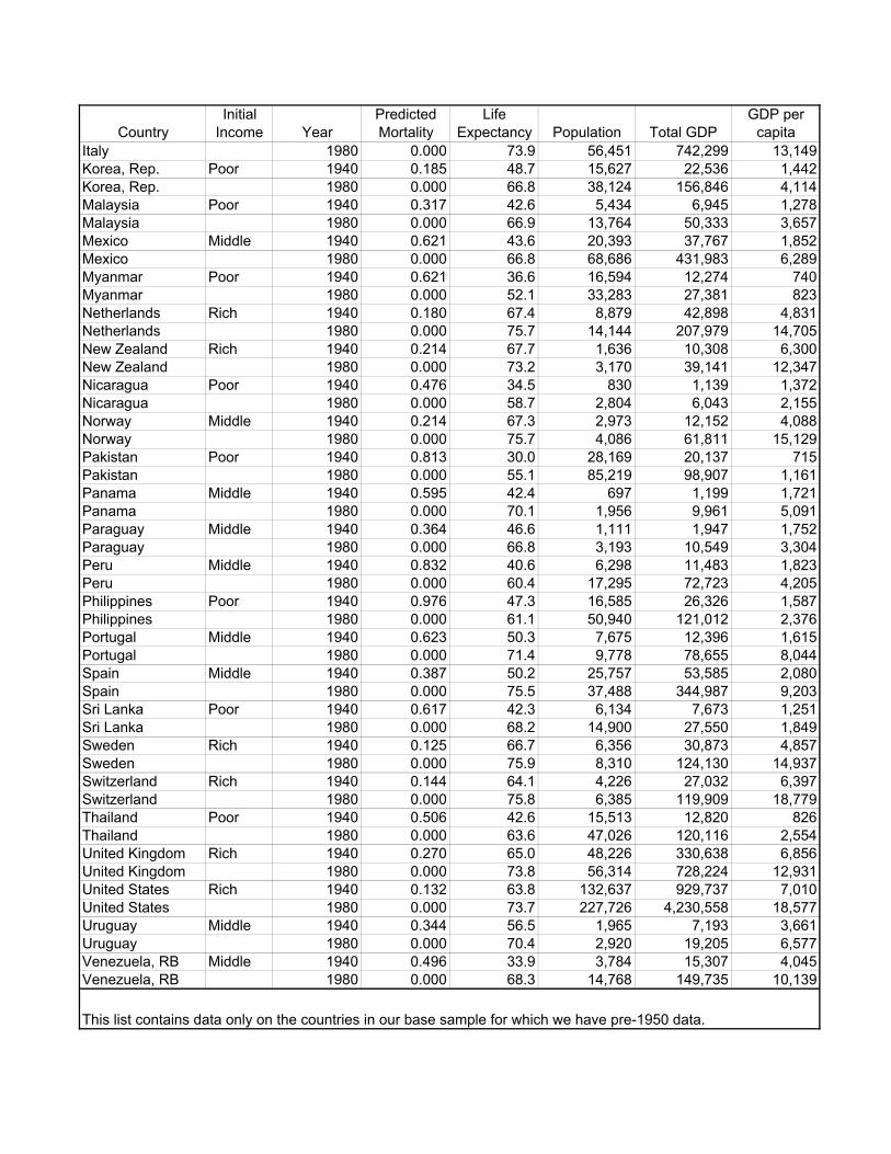
CountryInitial

Income YearPredicted Mortality

Life Expectancy Population Total GDP

GDP per capita

Italy 1980 0.000 73.9 56,451 742,299 13,149Korea, Rep. Poor 1940 0.185 48.7 15,627 22,536 1,442Korea, Rep. 1980 0.000 66.8 38,124 156,846 4,114Malaysia Poor 1940 0.317 42.6 5,434 6,945 1,278Malaysia 1980 0.000 66.9 13,764 50,333 3,657Mexico Middle 1940 0.621 43.6 20,393 37,767 1,852Mexico 1980 0.000 66.8 68,686 431,983 6,289Myanmar Poor 1940 0.621 36.6 16,594 12,274 740Myanmar 1980 0.000 52.1 33,283 27,381 823Netherlands Rich 1940 0.180 67.4 8,879 42,898 4,831Netherlands 1980 0.000 75.7 14,144 207,979 14,705New Zealand Rich 1940 0.214 67.7 1,636 10,308 6,300New Zealand 1980 0.000 73.2 3,170 39,141 12,347Nicaragua Poor 1940 0.476 34.5 830 1,139 1,372Nicaragua 1980 0.000 58.7 2,804 6,043 2,155Norway Middle 1940 0.214 67.3 2,973 12,152 4,088Norway 1980 0.000 75.7 4,086 61,811 15,129Pakistan Poor 1940 0.813 30.0 28,169 20,137 715Pakistan 1980 0.000 55.1 85,219 98,907 1,161Panama Middle 1940 0.595 42.4 697 1,199 1,721Panama 1980 0.000 70.1 1,956 9,961 5,091Paraguay Middle 1940 0.364 46.6 1,111 1,947 1,752Paraguay 1980 0.000 66.8 3,193 10,549 3,304Peru Middle 1940 0.832 40.6 6,298 11,483 1,823Peru 1980 0.000 60.4 17,295 72,723 4,205Philippines Poor 1940 0.976 47.3 16,585 26,326 1,587Philippines 1980 0.000 61.1 50,940 121,012 2,376Portugal Middle 1940 0.623 50.3 7,675 12,396 1,615Portugal 1980 0.000 71.4 9,778 78,655 8,044Spain Middle 1940 0.387 50.2 25,757 53,585 2,080Spain 1980 0.000 75.5 37,488 344,987 9,203Sri Lanka Poor 1940 0.617 42.3 6,134 7,673 1,251Sri Lanka 1980 0.000 68.2 14,900 27,550 1,849Sweden Rich 1940 0.125 66.7 6,356 30,873 4,857Sweden 1980 0.000 75.9 8,310 124,130 14,937Switzerland Rich 1940 0.144 64.1 4,226 27,032 6,397Switzerland 1980 0.000 75.8 6,385 119,909 18,779Thailand Poor 1940 0.506 42.6 15,513 12,820 826Thailand 1980 0.000 63.6 47,026 120,116 2,554United Kingdom Rich 1940 0.270 65.0 48,226 330,638 6,856United Kingdom 1980 0.000 73.8 56,314 728,224 12,931United States Rich 1940 0.132 63.8 132,637 929,737 7,010United States 1980 0.000 73.7 227,726 4,230,558 18,577Uruguay Middle 1940 0.344 56.5 1,965 7,193 3,661Uruguay 1980 0.000 70.4 2,920 19,205 6,577Venezuela, RB Middle 1940 0.496 33.9 3,784 15,307 4,045Venezuela, RB 1980 0.000 68.3 14,768 149,735 10,139

This list contains data only on the countries in our base sample for which we have pre-1950 data.

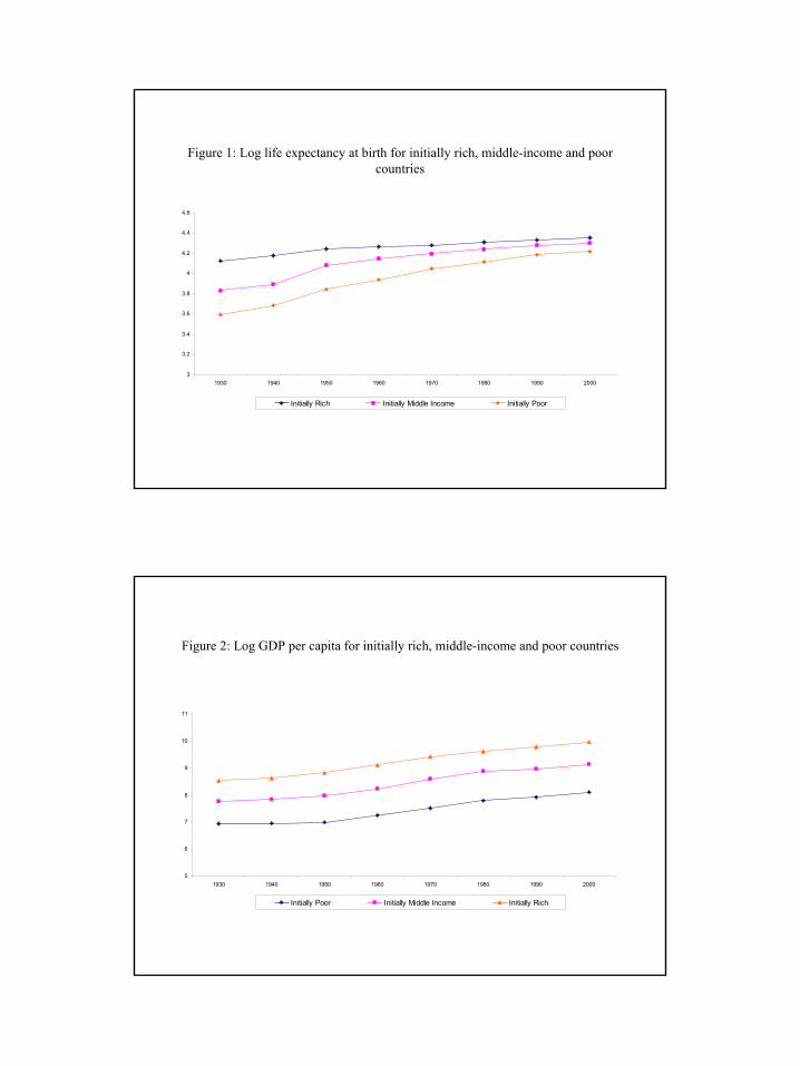
1

Figure 1: Log life expectancy at birth for initially rich, middle-income and poor countries

3

3.2

3.4

3.6

3.8

4

4.2

4.4

4.6

1930 1940 1950 1960 1970 1980 1990 2000

Initially Rich Initially Middle Income Initially Poor

Figure 2: Log GDP per capita for initially rich, middle-income and poor countries

5

6

7

8

9

10

11

1930 1940 1950 1960 1970 1980 1990 2000

Initially Poor Initially Middle Income Initially Rich

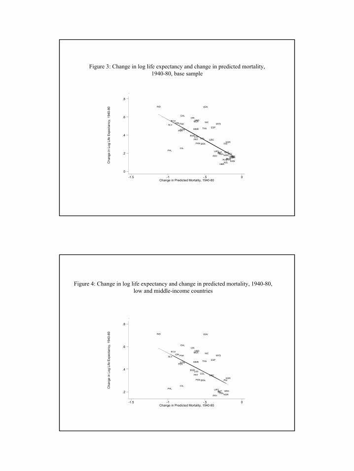
2

Figure 3: Change in log life expectancy and change in predicted mortality, 1940-80, base sample

.

Cha

nge

in L

og L

ife E

xpec

tanc

y, 1

940-

80

Change in Predicted Mortality, 1940-80-1.5 -1 -.5 0

0

.2

.4

.6

.8

ARG

AUS

AUT BEL

BGD

BRA

CANCHE

CHL

COL

CRI

DEUDNK

ECU

ESP

FIN

FRA

GBR

GRC

GTM

HNDIDN

IND

IRL

ITA

KOR

LKA

MEX

MMR

MYSNIC

NLDNOR

NZL

PAK

PAN

PER

PHL

PRT

PRY

SLV

SWE

THA

URY

USA

VEN

Figure 4: Change in log life expectancy and change in predicted mortality, 1940-80, low and middle-income countries

.

.

Cha

nge

in L

og L

ife E

xpec

tanc

y, 1

940-

80

Change in Predicted Mortality, 1940-80-1.5 -1 -.5 0

.2

.4

.6

.8

ARGAUT

BGD

BRA

CHL

COL

CRI

ECU

ESP

FIN

FRA

GRC

GTM

HNDIDN

IND

IRL

ITA

KOR

LKA

MEX

MMR

MYSNIC

NOR

PAK

PAN

PER

PHL

PRT

PRY

SLV

THA

URY

VEN

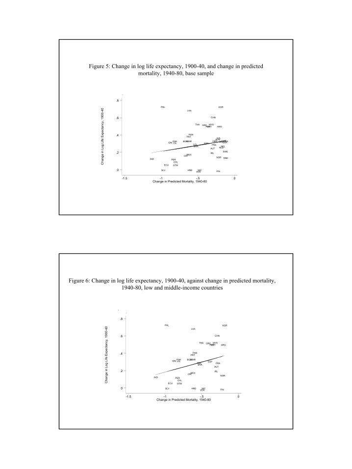
3

Figure 5: Change in log life expectancy, 1900-40, and change in predicted mortality, 1940-80, base sample

..

Cha

nge

in L

og L

ife E

xpec

tanc

y, 1

900-

40

Change in Predicted Mortality, 1940-80-1.5 -1 -.5 0

0

.2

.4

.6

.8

ARG

AUS

AUTBEL

BGD

BRA

CANCHE

CHL

CHN

COL

CRI

DEU

DNK

ECU

ESP

FIN

FRA

GBR

GRC

GTM

HND

IDN

IND

IRL

ITA

KORLKA

MEX

MMR

MYS

NIC

NLD

NOR

NZLPAK

PAN

PER

PHL

PRT

PRY

SLV

SWE

THAURY

USA

VEN

Figure 6: Change in log life expectancy, 1900-40, against change in predicted mortality,1940-80, low and middle-income countries

..

Cha

nge

in L

og L

ife E

xpec

tanc

y, 1

900-

40

Change in Predicted Mortality, 1940-80-1.5 -1 -.5 0

0

.2

.4

.6

.8

ARG

AUT

BGD

BRA

CHL

CHN

COL

CRI

ECU

ESP

FIN

FRA

GRC

GTM

HND

IDN

IND

IRL

ITA

KORLKA

MEX

MMR

MYS

NIC

NOR

PAK

PAN

PER

PHL

PRT

PRY

SLV

THAURY

VEN

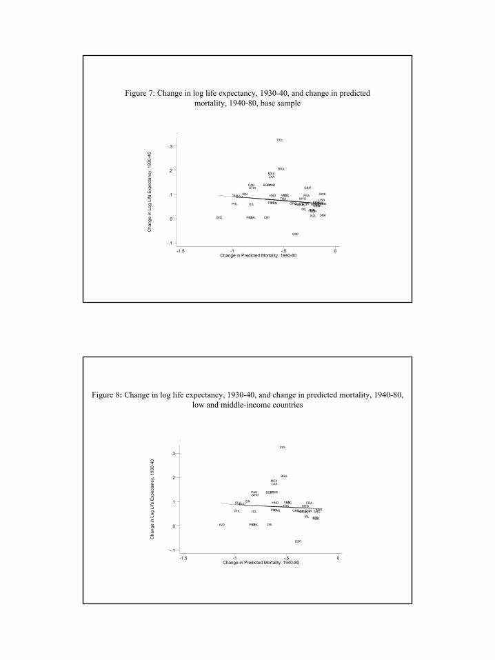
4

Figure 7: Change in log life expectancy, 1930-40, and change in predicted mortality, 1940-80, base sample

.

Cha

nge

in L

og L

ife E

xpec

tanc

y, 1

930-

40

Change in Predicted Mortality, 1940-80-1.5 -1 -.5 0

-.1

0

.1

.2

.3

ARG

AUSAUT BEL

BGD

BRA

CANCHE

CHL

CHN

COL

CRI

DEU

DNK

ECU

ESP

FIN

FRA

GBR

GRC

GTM

HNDIDN

IND

IRLITA

KOR

LKAMEX

MMR

MYSNIC

NLD

NORNZL

PAK

PAN

PER

PHL PRT PRY

SLV SWETHA

URYUSA

VEN

Figure 8: Change in log life expectancy, 1930-40, and change in predicted mortality, 1940-80, low and middle-income countries

.

.

Cha

nge

in L

og L

ife E

xpec

tanc

y, 1

930-

40

Change in Predicted Mortality, 1940-80-1.5 -1 -.5 0

-.1

0

.1

.2

.3

ARGAUT

BGD

BRA

CHL

CHN

COL

CRI

ECU

ESP

FIN

FRA

GRC

GTM

HNDIDN

IND

IRLITA

KOR

LKAMEX

MMR

MYSNIC

NOR

PAK

PAN

PER

PHL PRT PRY

SLVTHA

URY

VEN

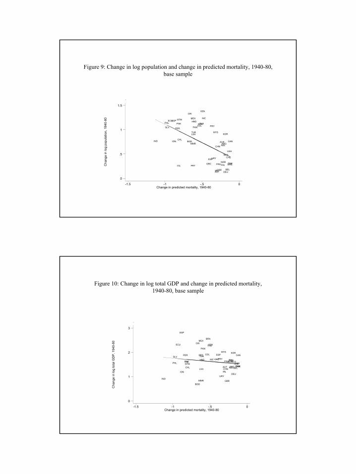
5

Figure 9: Change in log population and change in predicted mortality, 1940-80, base sample

.

Cha

nge

in lo

g po

pula

tion,

194

0-80

Change in predicted mortality, 1940-80-1.5 -1 -.5 0

0

.5

1

1.5

ARGAUS

AUTBEL

BGD

BRA

CAN

CHE

CHL

CHN

COL

CRI

DEU

DNK

ECU

ESP

FINFRA

GBR

GRC

GTMHND

IDNIND

IRL

ITA

KORLKA

MEX

MMR

MYS

NIC

NLD

NOR

NZL

PAKPANPER

PHL

PRT

PRY

SGP

SLV

SWE

THA

TUR

URY

USA

VEN

Figure 10: Change in log total GDP and change in predicted mortality, 1940-80, base sample

.

Cha

nge

in lo

g to

tal G

DP,

194

0-80

Change in predicted mortality, 1940-80-1.5 -1 -.5 0

0

1

2

3

ARG

AUS

AUT BEL

BGD

BRA

CAN

CHECHL

CHN

COL

CRI

DEU

DNK

ECU

ESP

FINFRA

GBR

GRC

GTM

HND

IDN

IND

IRL

ITA

KOR

LKA

MEX

MMR

MYS

NICNLDNOR

NZL

PAK

PAN

PER

PHL

PRT

PRY

SGP

SLV

SWE

THA

TUR

URY

USA

VEN

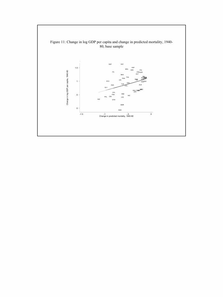
6

Figure 11: Change in log GDP per capita and change in predicted mortality, 1940-80, base sample

.

Cha

nge

in lo

g G

DP

per c

apita

, 194

0-80

Change in predicted mortality, 1940-80-1.5 -1 -.5 0

0

.5

1

1.5

ARG

AUS

AUT

BEL

BGD

BRA

CANCHE

CHLCHN

COL

CRIDEU

DNK

ECU

ESP

FINFRA

GBR

GRC

GTM

HND

IDN

IND

IRL

ITA

KOR

LKA

MEX

MMR

MYS

NIC

NLD

NOR

NZL

PAK

PAN

PER

PHL

PRT

PRY

SGP

SLV

SWETHA

TUR

URY

USAVEN