Discussion Papers in Economics

No. 2000/62

Dynamics of Output Growth, Consumption and Physical Capital in Two-Sector Models of Endogenous Growth

by

Farhad Nili

Department of Economics and Related Studies University of York

Heslington York, YO10 5DD

No. 2003/21

Corporate Bond Valuation with Both Expected and Unexpected Default

by

Marco Realdon

CORPORATE BOND VALUATIONWITH

BOTH EXPECTED AND UNEXPECTED

DEFAULT

Dr Marco Realdon

3/11/03

Abstract

This paper presents three variants of a tractable structural model in

which default may take place both expectedly and unexpectedly. The

model has the merit of predicting realistically high short term credit

spreads. Closed form solutions are provided for corporate bonds (and

default swaps) when interest rates are constant or stochastic and when

the bond recovery value is exogenous or endogenous to the model. The

analysis suggests that, in order for the observed short term yield spreads

on high grade corporate bonds to be compensation for credit risk, bond

holders must believe that a dramatic sudden plunge in the firm’s assets

value is possible, even if extremely unlikely.

Key words: corporate bond valuation, structural model, unexpected de-

fault, short term credit spreads, endogenous bond recovery value, plunge

1

of assets value.

JEL classification: G13;G33.

1 Introduction

This work presents closed form solutions for pricing corporate bonds and credit

default swaps using a structural model approach. Following Cathcart and El-

Jahel (2003), the specificity of the model is that default can occur in two different

ways, i.e. either when the value of the firm’s assets first drops to the level of the

default barrier, or when an unexpected sudden event causes the firm to default.

Within this framework closed form solutions are presented whereby the recovery

value of the bond upon default is either exogenous or endogenous to the model.

Under exogenous bond recovery value, the default free term structure can be

flat and constant or it can be stochastic.

When the default free term structure is flat and constant, the exogenous

bond recovery value is assumed to be a fraction of its face value. When the

default free short rate is stochastic, the exogenous recovery value of the bond is

assumed to be a fraction of its default free value, which is a typical assumption

in the presence of a stochastic default free term structure (see e.g. Longstaff

and Schwartz, 1995). This is a special case of the model by Cathcart and El-

Jahel (2003), for which a new closed form solution is presented. Under a flat and

constant term structure, the endogenous recovery value of the bond is a function

of the value of the debtor’s assets at the time of default. All these model variants

can provide a solution to a well know shortcoming of the "traditional" structural

2

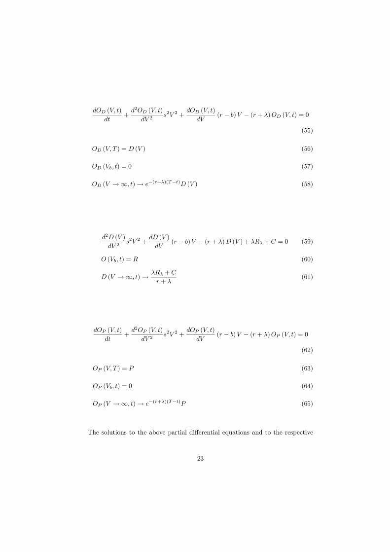
models of credit risk, in that they are capable to predict realistically high short

term credit spreads.

The analysis with endogenous debt recovery value suggests that, if the ob-

served short term yield spreads for high grade borrowers are compensation for

credit risk, bond holders must believe there is a tiny probability (e.g. less than

1% per annum) of a dramatic sudden drop in assets value, a drop which can

plunge assets value down to approximately the level of the default barrier.

1.1 Literature

In the last decade structural models and reduced form models of credit risk have

been "competing" to price default risky corporate bonds. Structural models

have the advantage of making effective use of balance sheet and equity price

information in a theoretically coherent way, but have been unable to generate

realistically high short term credit spreads. Reduced form models have been

able to generate realistically high short term credit spreads, but do not make

full use of firm specific information or are based on rating information which is

usually not timely or exhaustive.

The under-prediction of short term credit spreads by structural models is at

least partly due to the fact that empirically observed yield spreads on corporate

bonds incorporate a liquidity premium over and above a credit risk premium (see

e.g. Perraudin 2003). Moreover, such yield spreads may also partly be due to

the often less favorable tax treatment of corporate bond coupons with respect to

government bond coupons. Nether-the-less short term credit spreads predicted

3

by structural models still look disturbingly lower than observed corporate yield

spreads.

Recent literature on credit risk valuation, aware of the respective advantages

and disadvantages of structural models and reduced form models, has repeatedly

tried to reconcile the structural and the reduced form approaches in order to

achieve some sort of advantageous synthesis of two. Notable such examples

are Duffie and Lando (2001), who show how credit spreads are affected by the

often incomplete accounting information available to bond holders, and Zhou

(2001), who assumes that the value of the firm’s assets follows a jump diffusion

process and values bonds through simulation. These two models are capable

of predicting higher short term credit spreads than implied by usual structural

models at the expense of model tractability. Alternatively, the best practice,

e.g. Pan (2001), has assumed a stochastic default barrier capable to predict

non-negligible short term credit spreads on corporate bonds. Pan’s model as

well as Duffie and Lando’s have the drawback of predicting excessively high

short term spreads when default is likely and the bond is close to maturity.

This paper is more close in spirit to Cathcart and El-Jahel’s (2003) in that

both expected and unexpected default can take place. But, unlike in Cathcart

and El-Jahel, full closed form solutions are derived when the default hazard

rate is constant, when the default free interest rate is constant or stochastic and

when the recovery value of the defaulted bond is endogenous.

Hereafter, section 2 proposes new closed form solutions for bond and default

swap values under constant and stochastic interest rates given that the recovery

4

value of the defaulted bond is exogenous. Section 3 proposes a closed form solu-

tion for bond value under constant interest rates whereby the recovery value of

the defaulted bond depends on the firm’s assets value at the time of unexpected

default.

2 The bond valuationmodel with exogenous debt

recovery value

The bond valuation model assumptions are standard. The model assumes uni-

versal risk neutrality. The firm’s assets value risk neutral process follows a

geometric Brownian motion

dV = (r − b) · V · dt+ s · V · dz (1)

where r is the default free short interest rate assumed constant over time, where

b is the assets pay-out ratio, where s is the assets volatility parameter, where dz

is the differential of a Wiener process; b and s are are constant. The firm has

issued a bond security with value of D (V, t), with face value of P , with maturity

of T and yearly coupon flow (assumed to be continuously paid) of C. Default

can occur in an expected way the first time V drops to the level Vb. Thereupon

the recovery value of D (V, t), denoted by R, is an exogenous fraction α of the

bond face value P , i.e. R = αP with 0 ≤ α ≤ 1.

Default can occur also in an unexpected way in any infinitesimal time period

5

dt. In any period dt there is a probability λdt that default may be unexpectedly

precipitated causing D (V, t) to fall to the constant recovery value Rλ = α1P ,

where again 0 ≤ α1 ≤ 1. Thus R need not equal Rλ. Note that in this section

the bond recovery value upon default is an exogenous fraction of the par value

of the bond. Different recovery assumptions will be made later in the paper.

The event that triggers unexpected default is a completely unexpected event

that is independent of the market value of the firm’s assets V , such as may be the

discovery of substantial misgivings in the firm’s accounts. Employing standard

valuation arguments, we know that the value D (V, t) of the corporate bond

satisfies the following equation

dD (V, t)

dt+

d2D (V, t)

dV 2s2V 2 +

dD (V, t)

dV(r − b)V − (r + λ)D (V, t) + C + λRλ = 0

(2)

D (V, T ) = P (3)

D (Vb, t) = R (4)

D (V →∞, t)→ λRλ + C

r + λ

³1− e−(r+λ)(T−t)

´+ e−(r+λ)(T−t)P (5)

Equation 2 reflects the facts that a continuous coupon flow is received by

bond holders at the yearly rate C, that the bond is subject to unexpected default

with constant hazard rate λ, that the bond holders recover R upon expected

default and Rλ upon unexpected default. Condition 3 is the terminal condition

if the debtor is solvent. Condition 4 sets the recovery value of the bond when the

6

default barrier is first reached. Condition 5 reflects the fact that, as the firm’s

assets become very valuable, default can take place only in an unexpected way.

The right hand side of condition 5 is the value of the bond when only unexpected

default can occur with intensity λ.

In deriving equation 2 universal risk neutrality is assumed, but such assump-

tion does not seem restrictive. In fact expected default is driven by the dynamics

of assets value V , which can be replicated at least in principle so to make the

market complete. And we know from Harrison and Kreps (1979) that market

completeness is tantamount to the risk neutrality assumption. Moreover λ is

both the real and the risk-neutral intensity of unexpected default. In fact the

risk of unexpected default commands no premium, since such risk is assumed to

have no systematic component, unexpected default being a complete surprise.

The solution to equation 2 and to the respective conditions is

D (V, t) = D (V )−OD (V, t) +OP (V, t) (6)

D (V ) =λRλ + C

r + λ+

µ−λRλ + C

r + λ+R

¶µV

Vb

¶q(7)

q =− ¡r − b− 1

2s2¢−q¡r − b− 1

2s2¢2+ 2 (r + λ) s2

s2(8)

7

OD (V, t) =λRλ + C

r + λe−(r+λ)(T−t) · Ω

µd

µV

Vb, 1

¶, d

µVbV, 1

¶, 0, 1

¶(9)

− −λRλ+Cr+λ +R

(Vb)q e(−(r+λ)+n(q))(T−t) · Ω

µd

µV

Vb, q

¶, d

µVbV, q

¶, q, q

¶

OP (V, t) = P · e−(r+λ)(T−t) · Ωµd

µV

Vb, 1

¶, d

µVbV, 1

¶, 0, 1

¶(10)

n (w) = (r − b)w +1

2w (w − 1) s2 (11)

d (z,w) =w ln (z) +

¡n (w) + 1

2s2w2

¢(T − t)

ws√T − t

(12)

Ω (k1, k2, k3, w) = V k3N (k1)−µ

V

VB

¶−2n(w)w·s2

(VB)k3 N (k2) (13)

These formulae allow to derive a closed form solution also for the value of a

credit default swap S (V, t), which pays P − Rλ in case of unexpected default

and P − R in case of expected default before time T , and which requires the

protection buyer (bondholder) to continuously pay a constant premium at the

yearly rate Cs. Then the value of one such credit default swap for the protection

buyer is

S (V, t) = S (V )−OS (V, t) (14)

8

S (V ) =λ (P −Rλ)− Cs

r + λ+

µ−λ (P −Rλ)− Cs

r + λ+R

¶µV

Vb

¶q(15)

q =− ¡r − b− 1

2s2¢−q¡r − b− 1

2s2¢2+ 2 (r + λ) s2

s2(16)

OS (V, t) =λ (P −Rλ)− Cs

r + λe−(r+λ)(T−t) · Ω

µd

µV

Vb, 1

¶, d

µVbV, 1

¶, 0, 1

¶(17)

−λ(P−Rλ)−Cs

r+λ +R

(Vb)q e(−(r+λ)+n(q))(T−t) · Ω

µd

µV

Vb, q

¶, d

µVbV, q

¶, q, q

¶

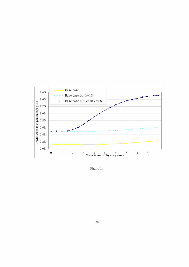
Figure 1 shows the model predicted term structure of credit spreads. The

figure shows that the advantage of allowing both expected and unexpected de-

fault to occur is that short term credit spreads are realistically high. The figure

assumes a base case with V = 100, Vb = 30, b = 5%, σ = 20%, r = 4%, T = 10,

F = 30, C = 5%·F , λ = 0.25%, Rλ = 0.5 and R = 0.5. Notice that if λ = 0.25%

the unexpected drop in assets value takes place every 1λ = 400 years on average.

The figure shows that as λ increases so that unexpected default becomes

more likely, credit spreads on even high grade bonds widen. Such are the bonds

for which structural models usually predict too low short term credit spreads.

So far a flat and constant term structure of default free interest rates has

been assumed. Now this assumption is relaxed.

9

2.1 When default free interest rates are stochastic

A closed form solutions for corporate bonds valuation is now presented when

the term structure of interest rates is stochastic and, as before, default can be

either expected or unexpected. In keeping with other structural models that

assume a stochastic default free term structure, this section assumes that debt

holders recover a fraction of the default free value of the cash flows promised by

the bond ("recovery of Treasury" assumption, see e.g. Longstaff and Schwartz

(1995)).

In this section we also assume that the market in incomplete, so that the

stochastic dynamics of the firm’s assets value cannot be replicated by trading

in market securities. If follows that now the risk neutral process for V is

dV = V · (m− λV · s) · dt+ V · s · dz (18)

where λV is a constant that denotes the market price of V risk. Such risk

neutral process is assumed also in Cathcart and El-Jahel (2003). Moreover, the

risk neutral process for r is now assumed to follow a generic process

dr = u (r, t) + σ (r, t) dzr

where u (r, t) and σ (r, t) are continuously differetiable functions of the short

default free interest rate r and of time t, and where dzr is the differential of a

Wiener process. V and r are instantaneously uncorrelated, i.e. E (dV · dr) = 0

or E (dz · dzr) = 0, as is assumed also in Cathcart and El-Jahel (2003). Then,

10

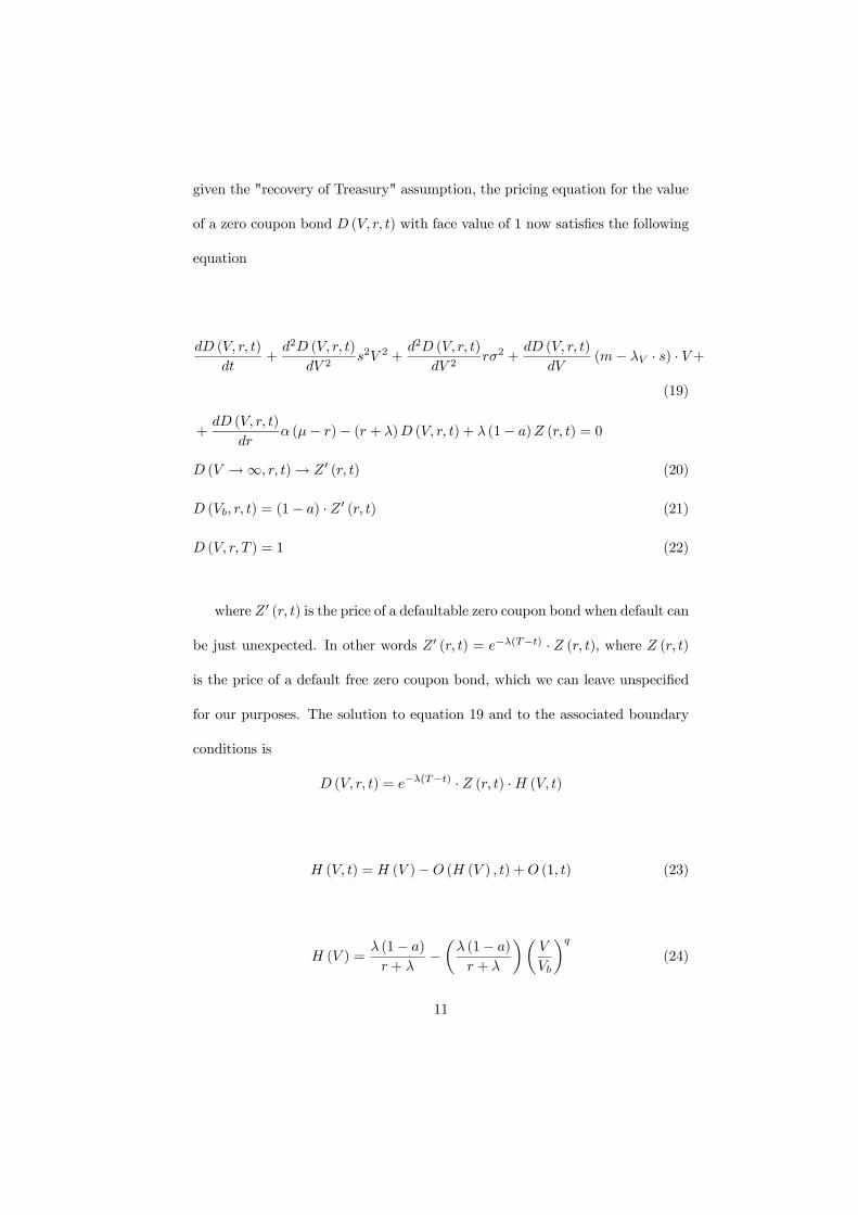
given the "recovery of Treasury" assumption, the pricing equation for the value

of a zero coupon bond D (V, r, t) with face value of 1 now satisfies the following

equation

dD (V, r, t)

dt+

d2D (V, r, t)

dV 2s2V 2 +

d2D (V, r, t)

dV 2rσ2 +

dD (V, r, t)

dV(m− λV · s) · V+

(19)

+dD (V, r, t)

drα (µ− r)− (r + λ)D (V, r, t) + λ (1− a)Z (r, t) = 0

D (V →∞, r, t)→ Z0 (r, t) (20)

D (Vb, r, t) = (1− a) · Z0 (r, t) (21)

D (V, r, T ) = 1 (22)

where Z0 (r, t) is the price of a defaultable zero coupon bond when default can

be just unexpected. In other words Z0 (r, t) = e−λ(T−t) · Z (r, t), where Z (r, t)

is the price of a default free zero coupon bond, which we can leave unspecified

for our purposes. The solution to equation 19 and to the associated boundary

conditions is

D (V, r, t) = e−λ(T−t) · Z (r, t) ·H (V, t)

H (V, t) = H (V )−O (H (V ) , t) +O (1, t) (23)

H (V ) =λ (1− a)

r + λ−µλ (1− a)

r + λ

¶µV

Vb

¶q(24)

11

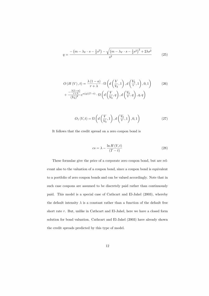
q =− ¡m− λV · s− 1

2s2¢−q¡m− λV · s− 1

2s2¢2+ 2λs2

s2(25)

O (H (V ) , t) =λ (1− a)

r + λ· Ωµd

µV

Vb, 1

¶, d

µVbV, 1

¶, 0, 1

¶(26)

+−λ(1−a)

r+λ

(Vb)q en(q)(T−t) · Ω

µd

µV

Vb, q

¶, d

µVbV, q

¶, q, q

¶

O1 (V, t) = Ω

µd

µV

Vb, 1

¶, d

µVbV, 1

¶, 0, 1

¶(27)

It follows that the credit spread on a zero coupon bond is

cs = λ− lnH (V, t)(T − t)

(28)

These formulae give the price of a corporate zero coupon bond, but are rel-

evant also to the valuation of a coupon bond, since a coupon bond is equivalent

to a portfolio of zero coupon bonds and can be valued accordingly. Note that in

such case coupons are assumed to be discretely paid rather than continuously

paid. This model is a special case of Cathcart and El-Jahel (2003), whereby

the default intensity λ is a constant rather than a function of the default free

short rate r. But, unlike in Cathcart and El-Jahel, here we have a closed form

solution for bond valuation. Cathcart and El-Jahel (2003) have already shown

the credit spreads predicted by this type of model.

12

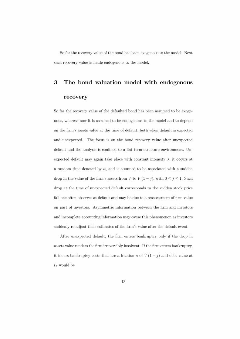
So far the recovery value of the bond has been exogenous to the model. Next

such recovery value is made endogenous to the model.

3 The bond valuation model with endogenous

recovery

So far the recovery value of the defaulted bond has been assumed to be exoge-

nous, whereas now it is assumed to be endogenous to the model and to depend

on the firm’s assets value at the time of default, both when default is expected

and unexpected. The focus is on the bond recovery value after unexpected

default and the analysis is confined to a flat term structure environment. Un-

expected default may again take place with constant intensity λ, it occurs at

a random time denoted by tλ and is assumed to be associated with a sudden

drop in the value of the firm’s assets from V to V (1− j), with 0 ≤ j ≤ 1. Such

drop at the time of unexpected default corresponds to the sudden stock price

fall one often observes at default and may be due to a reassessment of firm value

on part of investors. Asymmetric information between the firm and investors

and incomplete accounting information may cause this phenomenon as investors

suddenly re-adjust their estimates of the firm’s value after the default event.

After unexpected default, the firm enters bankruptcy only if the drop in

assets value renders the firm irreversibly insolvent. If the firm enters bankruptcy,

it incurs bankruptcy costs that are a fraction a of V (1− j) and debt value at

tλ would be

13

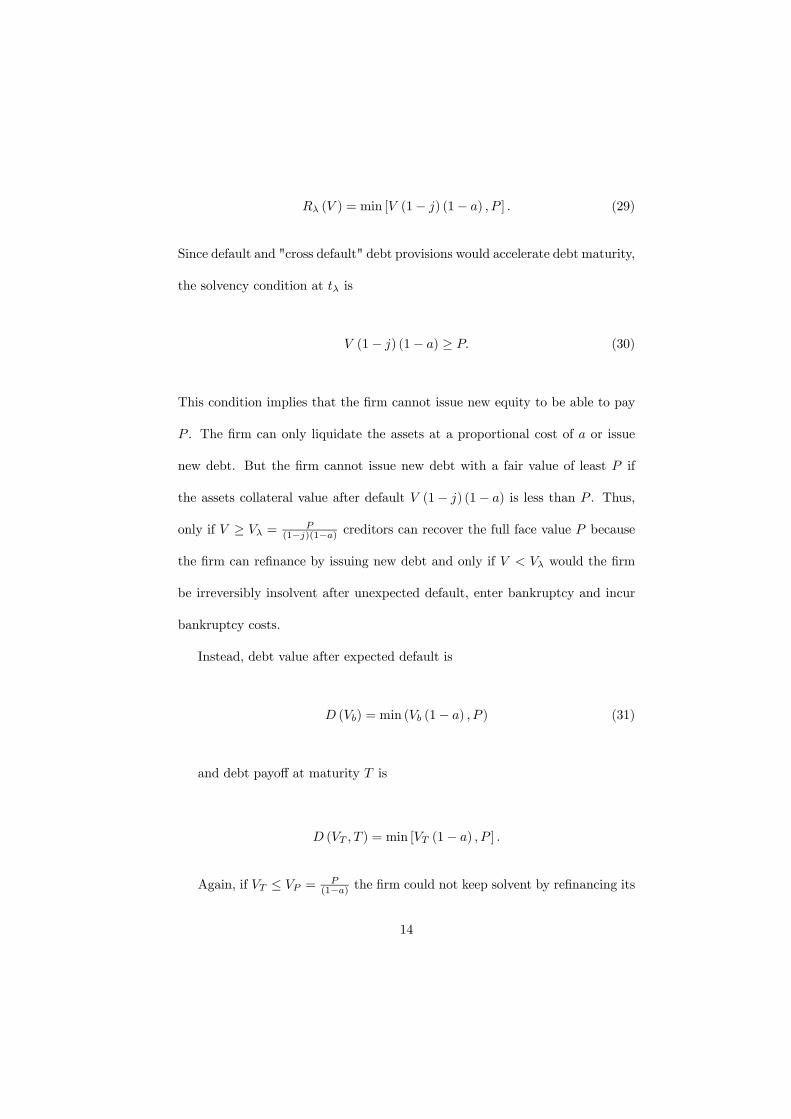
Rλ (V ) = min [V (1− j) (1− a) , P ] . (29)

Since default and "cross default" debt provisions would accelerate debt maturity,

the solvency condition at tλ is

V (1− j) (1− a) ≥ P. (30)

This condition implies that the firm cannot issue new equity to be able to pay

P . The firm can only liquidate the assets at a proportional cost of a or issue

new debt. But the firm cannot issue new debt with a fair value of least P if

the assets collateral value after default V (1− j) (1− a) is less than P . Thus,

only if V ≥ Vλ =P

(1−j)(1−a) creditors can recover the full face value P because

the firm can refinance by issuing new debt and only if V < Vλ would the firm

be irreversibly insolvent after unexpected default, enter bankruptcy and incur

bankruptcy costs.

Instead, debt value after expected default is

D (Vb) = min (Vb (1− a) , P ) (31)

and debt payoff at maturity T is

D (VT , T ) = min [VT (1− a) , P ] .

Again, if VT ≤ VP =P

(1−a) the firm could not keep solvent by refinancing its

14

debt through liquidation of its assets or issuance of new debt. Again the firm

cannot issue new equity. Typically VP would be higher than Vb.

Employing standard valuation arguments (see e.g. Wilmott 1998 at chap-

ter 26) and assuming that the value of the firm’s assets follows the process of

equation 1 we can now re-write the debt pricing equation as

dD (V, t)

dt+

d2D (V )

dV 2s2V 2 +

dD (V )

dV(r − b+ λj)V − (r + λ)D (V ) + C + λRλ (V ) = 0

(32)

D (VT , T ) = VT (1− a) · 1VT≤VP + P · 1VT>VP (33)

D (Vb, t) = min (Vb (1− a) , P ) (34)

D (V →∞, t)→ C + λP

r + λ

³1− e−(r+λ)(T−t)

´+ e−(r+λ)(T−t)P (35)

This is the same model as in section one, but the recovery value after unexpected

default is now endogenous. The solution to 32 is:

D (V, t) = D (V )−ODh(V, t)−ODl

(V, t) +OP (V, t) (36)

D (V ) = Dh (V ) · 1V >VP +Dl (V ) · 1V≤VP (37)

where 1x>y is the indicator function such that, 1x>y = 1 if x > y and

1x>y = 0 if x ≤ y;

15

Dh (V ) =λP + C

r + λ+

µ−λP + C

r + λ+Dl (Vλ, t)

¶µV

Vλ

¶q2(38)

Dl (V ) =λ (1− a) (1− j)V + C

b+ λ+ k1V

q1 + k2Vq2 (39)

q1 =− ¡r − b+ λj − s2

¢+

q(r − b+ λj − s2)

2+ 4s2 (r + λ)

2s2(40)

q2 =− ¡r − b+ λj − s2

¢−q(r − b+ λj − s2)2 + 4s2 (r + λ)

2s2(41)

ODh (V, t) =λ+ C

r + λe−(r+λ)(T−t) · Ω

µd−

µV

Vb

¶, d−

µV 2b

V ·Vλ

¶, 0, 1

¶(42)

+

³−λ+C

r+λ +Dl (Vλ, t)´

(Vλ)q2 · e(−(r+λ)+n(q2))(T−t) · Ω

µd

µV

Vb, q2

¶, d

µV 2b

V ·Vλ , q2

¶, q2, q2

¶

16

ODl (V, t) =C

b+ λe−(r+λ)(T−t) · (43)·

Ω

µd−

µV

Vb

¶, d−

µV 2b

V ·VP

¶, 0, 1

¶− Ω

µd−

µV

Vb

¶, d−

µV 2b

V ·Vλ

¶, 0, 1

¶¸(44)

+λ (1− a) (1− j)

b+ λe−λ(T−t) ··

Ω

µd

µV

Vb, 1

¶, d

µV 2b

V ·VP , 1¶, 1, 1

¶− Ω

µd

µV

Vb, 1

¶, d

µV 2b

V ·Vλ , 1¶, 1, 1

¶¸(45)

+k1 · e(−(r+λ)+n(q1))(T−t) ··Ω

µd

µV

Vb, q1

¶, d

µV 2b

V ·VP , q1

¶, q1, q1

¶− Ω

µd

µV

Vb, q1

¶, d

µV 2b

V ·Vλ , q1

¶, q1, q1

¶¸(46)

+k2 · e(−(r+λ)+n(q2))(T−t) ··Ω

µd

µV

Vb, q2

¶, d

µV 2b

V ·VP , q2

¶, q2, q2

¶− Ω

µd

µV

Vb, q2

¶, d

µV 2b

V ·Vλ , q2

¶, q2, q2

¶¸(47)

OP (V, t) = P · e−(r+λ)(T−t) · Ωµd

µV

Vb, 1

¶, d

µV 2b

V ·VP , 1¶, 0, 1

¶(48)

+e−λ(T−t) · (1− a) · (49)·Ω

µd

µV

Vb, 1

¶, d

µVbV, 1

¶, 1, 1

¶− Ω

µd

µV

Vb, 1

¶, d

µV 2b

V ·VP , 1¶, 1, 1

¶(50)

where

k1 =−k2V q2

b + (1− a)Vb − λ(1−a)(1−j)b+λ Vb

V q1b

(51)

k2 =

³− λP

r+λ +Dl (Vλ, t)´q2

1Vλ− λ(1−a)(1−j)

b+λ − −k2Vq2b +(1−a)Vb−λ(1−a)(1−j)

b+λ Vb

Vq1b

q1Vq1−1

q2V q2−1 (52)

17

and where d− (x) =ln(x)+(r−b+λj+ 1

2s2)(T−t)

s√T−t and where Vλ = P

(1−j)(1−a) .

We could reinterpret this model also as follows. At tλ assets value falls

because accounting mis-givings are detected and the true assets value becomes

known to the market. This event gives debt holders the right to accelerates

debt maturity, which does precipitate the firm’s insolvency if the firm cannot

refinance by issuing new debt in order to pay P .

3.1 Comparative statics

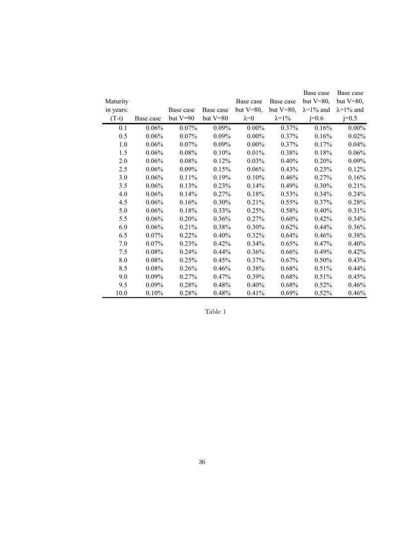
Comparative statics using the model in this section are summarised in Table 1.

The base case scenario assumes V = 100, Vb = 30, b = 5%, σ = 20%, r = 4%,

T = 10, F = 30, C = 5% · F , a = 20%, λ = 0.25%, j = 0.7.

In the base case credit spreads are very low but they short term spreads

and long term spreads are similar in magnitude. The third and fourth columns

show how the credit spreads increase as V lowers to 90 or to 80, ceteris paribus.

Notice how short term spreads do not vanish even for short maturities. The fifth

and sixth columns show how the magnitude of the unexpected default intensity

λ drives the level of short term credit spreads. When λ = 0, short term spreads

vanish because unexpected default is ruled out. The two rightmost columns

show that a dramatic downwards jump in assets value is required to prevent

short term spreads form vanishing. When j = 0.5 short term spreads are much

lower than long term spreads and in fact nearly disappear despite the possibility

of unexpected default. This highlights that it is only an unexpected dramatic

fall in assets value, even if very unlikely, that can boost short term spreads, i.e.

18

justify higher short term credit spreads than the spreads predicted by "classic"

structural models. In fact, creditors can recover the full face value of debt if

assets are valuable enough after unexpected default (i.e. if Vλ > P(1−j)(1−a) ),

so that short term spreads for high credits are tend to zero despite possible

unexpected default.

We can conclude that when the bond recovery value is endogenous in that

it is a function of the firm’s assets value, unexpected default can explain real-

istically high short term credit spreads for low grade debtors, but less so for

high grade debtors. If the observed short term yield spreads on high grade

corporate bonds are compensation for credit risk, investors must gauge that un-

expected default is possible, even if it is unlikely, and that it is associated with

an exceptional drop in assets value.

3.2 Random jump in assets value and random bankruptcy

costs

The model of this section can be easily adapted if the size of the assets value

jump j is random and distributed according to a discrete probability distribu-

tion. Suppose j is distributed such that j = i with probability p (i), i is such

that 0 ≤ i ≤ n ≤ 1 and Pni=0 p (i) = 1. Then, denoting with D (V, t, j∗) the

bond value when j is distributed as just described, from the concavity of Rλ (V )

with respect to j it follows that

D (V, t, j∗) =nXi=0

p (i) ·D (V, t, i) ≤ D (V, t,E (i)) (53)

19

where D (V, t, i) is the bond value as per equation 36 when j is certain and

equal to i and where D (V, t, E (i)) is the bond value when j is equal to the

expected value E (i) with certainty. Note that E (i) =Pn

i=0 i · p (i). In a

similar way it is possible to adapt the proposed model when the bankruptcy

cost parameter a is random and the distribution for a is a discrete one.

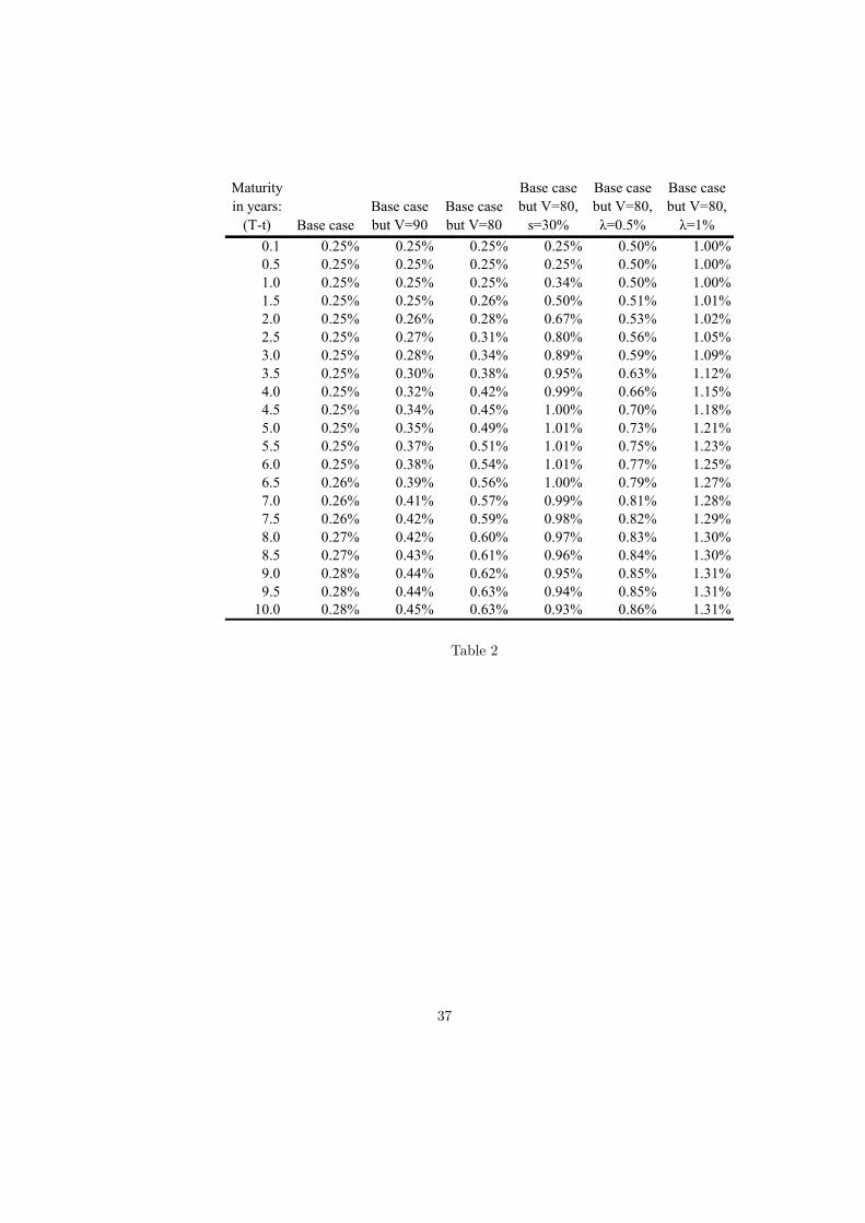
Table 2 shows model predicted credit spreads as j is uniformly distributed

such that i = 0100 ,

1100 ,

2100 , ..up to

100100 and p (i) = 1

101 for any i. The uniform

distribution corresponds to maximum uncertainty about the magnitude of the

drop in assets value. Table 2 assumes the same parameters as in Table 1 and

shows how, when j is uniformly distributed, high short term credit spreads are

possible and they are driven by the magnitude of the default intensity λ. It

is the extreme uncertainty about j that causes credit spreads in Table 2 to be

higher than in Table 1. The fifth column of Table 2 also shows that higher assets

volatility can significantly increase credit spreads for bond maturities beyond

one year or so.

Overall, the uncertainty about the magnitude of the unexpected jump in

assets value can contribute to increase the model predicted credit spreads up to

the empirically observed levels of yield spreads between corporate and Treasury

bonds.

20

4 Conclusion

This paper has presented three variants of a structural model of credit risk in

closed form, whereby both expected and unexpected defaults may take place.

Closed form solutions have been provided for corporate bonds and credit default

swaps, both when interest rates are constant and stochastic, and both when the

recovery value of the bond after default is exogenous or endogenous to the model.

With exogenous bond recovery value, the model has the merit of predicting

non negligible credit spreads even for short maturities and even for the best

credits. This is true both under constant and under stochastic interest rates and

the reason is that unexpected default increases credit spreads of all maturities.

But this is often not true of short term credit spreads with endogenous bond

recovery value.

When the bond recovery value is endogenous, unexpected default may be

associated with a sudden significant drop in the firm’s assets value, as is sug-

gested by the sharp drop in stock price one often observes at the time of default.

Asymmetric information between the firm and investors and less than transpar-

ent accounting information may explain this phenomenon, as the drop in assets

value at default may correspond to a reassessment of firm value on part of in-

vestors. Such drop can render a good credit economically insolvent and cause

the firm’s assets to be insufficient to fully satisfy the claim of bondholders after

default. But such drop must be exceptionally large to render a good credit insol-

vent. Overall, when recovery value is endogenous, unexpected default together

with a simultaneous sudden and potentially large drop in the firm’s assets value

21

can explain why short term credit spreads should be higher than "classic" struc-

tural models of credit risk do predict. Moreover, extreme uncertainty about the

magnitude of the potential plunge in assets value contributes to boost model

predicted short term credit spreads.

High short term credit spreads seem plausible for low grade debtors, but

less so for high grade debtors. If the observed short term yield spreads for high

grade borrowers are compensation for credit risk, investors must believe there is

a tiny probability, e.g. around 0.25% per annum, of a dramatic sudden plunge

in assets value down to approximately the default barrier level.

A When interest rates are constant

The solution to equation 2 and to the respective boundary conditions is

D (V, t) = D (V )−OD (V, t) +OP (V, t) (54)

where

22

dOD (V, t)

dt+

d2OD (V, t)

dV 2s2V 2 +

dOD (V, t)

dV(r − b)V − (r + λ)OD (V, t) = 0

(55)

OD (V, T ) = D (V ) (56)

OD (Vb, t) = 0 (57)

OD (V →∞, t)→ e−(r+λ)(T−t)D (V ) (58)

d2D (V )

dV 2s2V 2 +

dD (V )

dV(r − b)V − (r + λ)D (V ) + λRλ + C = 0 (59)

O (Vb, t) = R (60)

D (V →∞, t)→ λRλ + C

r + λ(61)

dOP (V, t)

dt+

d2OP (V, t)

dV 2s2V 2 +

dOP (V, t)

dV(r − b)V − (r + λ)OP (V, t) = 0

(62)

OP (V, T ) = P (63)

OP (Vb, t) = 0 (64)

OP (V →∞, t)→ e−(r+λ)(T−t)P (65)

The solutions to the above partial differential equations and to the respective

23

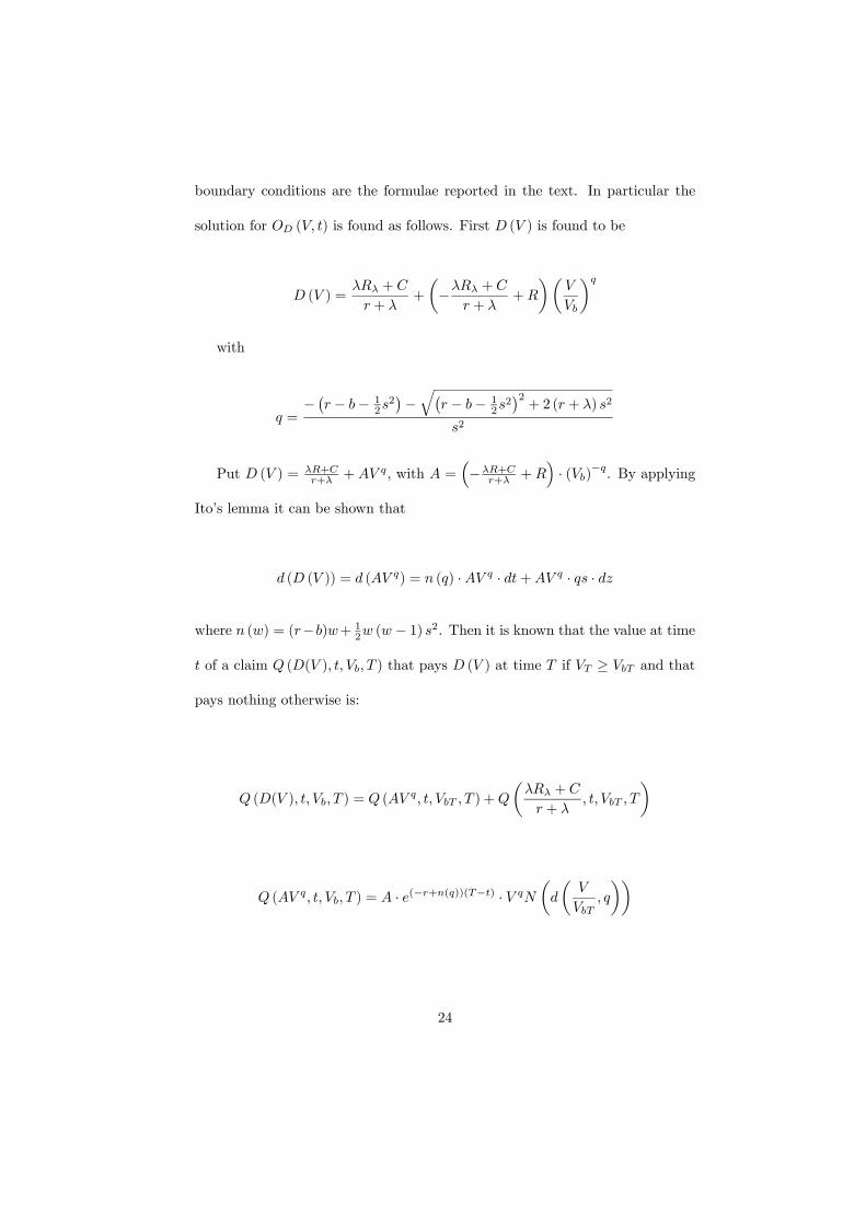
boundary conditions are the formulae reported in the text. In particular the

solution for OD (V, t) is found as follows. First D (V ) is found to be

D (V ) =λRλ + C

r + λ+

µ−λRλ + C

r + λ+R

¶µV

Vb

¶q

with

q =− ¡r − b− 1

2s2¢−q¡r − b− 1

2s2¢2+ 2 (r + λ) s2

s2

Put D (V ) = λR+Cr+λ + AV q, with A =

³−λR+C

r+λ +R´· (Vb)−q. By applying

Ito’s lemma it can be shown that

d (D (V )) = d (AV q) = n (q) ·AV q · dt+AV q · qs · dz

where n (w) = (r−b)w+ 12w (w − 1) s2. Then it is known that the value at time

t of a claim Q (D(V ), t, Vb, T ) that pays D (V ) at time T if VT ≥ VbT and that

pays nothing otherwise is:

Q (D(V ), t, Vb, T ) = Q (AV q, t, VbT , T ) +Q

µλRλ + C

r + λ, t, VbT , T

¶

Q (AV q, t, Vb, T ) = A · e(−r+n(q))(T−t) · V qN

µd

µV

VbT, q

¶¶

24

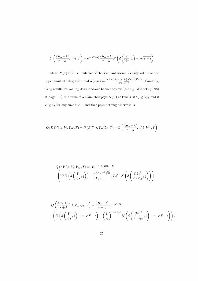
Q

µλRλ + C

r + λ, t, Vb, T

¶= e−r(T−t)

λRλ + C

r + λN

µd

µV

VbT, 1

¶− s√T − t

¶

where N (x) is the cumulative of the standard normal density with x as the

upper limit of integration and d (z,w) =w ln(z)+(n(w)+ 1

2s2w2)(T−t)

ws√T−t . Similarly,

using results for valuing down-and-out barrier options (see e.g. Wilmott (1998)

at page 192), the value of a claim that pays D (V ) at time T if VT ≥ VbT and if

Vt ≥ Vb for any time t < T and that pays nothing otherwise is:

Q (D (V ) , t, Vb, VbT , T ) = Q (AV q, t, Vb, VbT , T ) +Q

µλRλ + C

r + λ, t, Vb, VbT , T

¶

Q (AV q, t, Vb, VbT , T ) = Ae(−r+n(q))(T−t)

·V qN

µd

µV

VbT, q

¶¶−µV

Vb

¶−2n(q)q·s2

(Vb)q ·N

Ãd

Ã(Vb)

2

V · VbT , q!!

Q

µλRλ + C

r + λ, t, Vb, VbT , T

¶=

λRλ + C

r + λe−r(T−t)

·ÃN

µd

µV

VbT, 1

¶− s ·√T − t

¶−µV

Vb

¶1−2 r−bs2

N

Ãd

Ã(Vb)

2

V · VbT , 1!− s ·√T − t

!!.

25

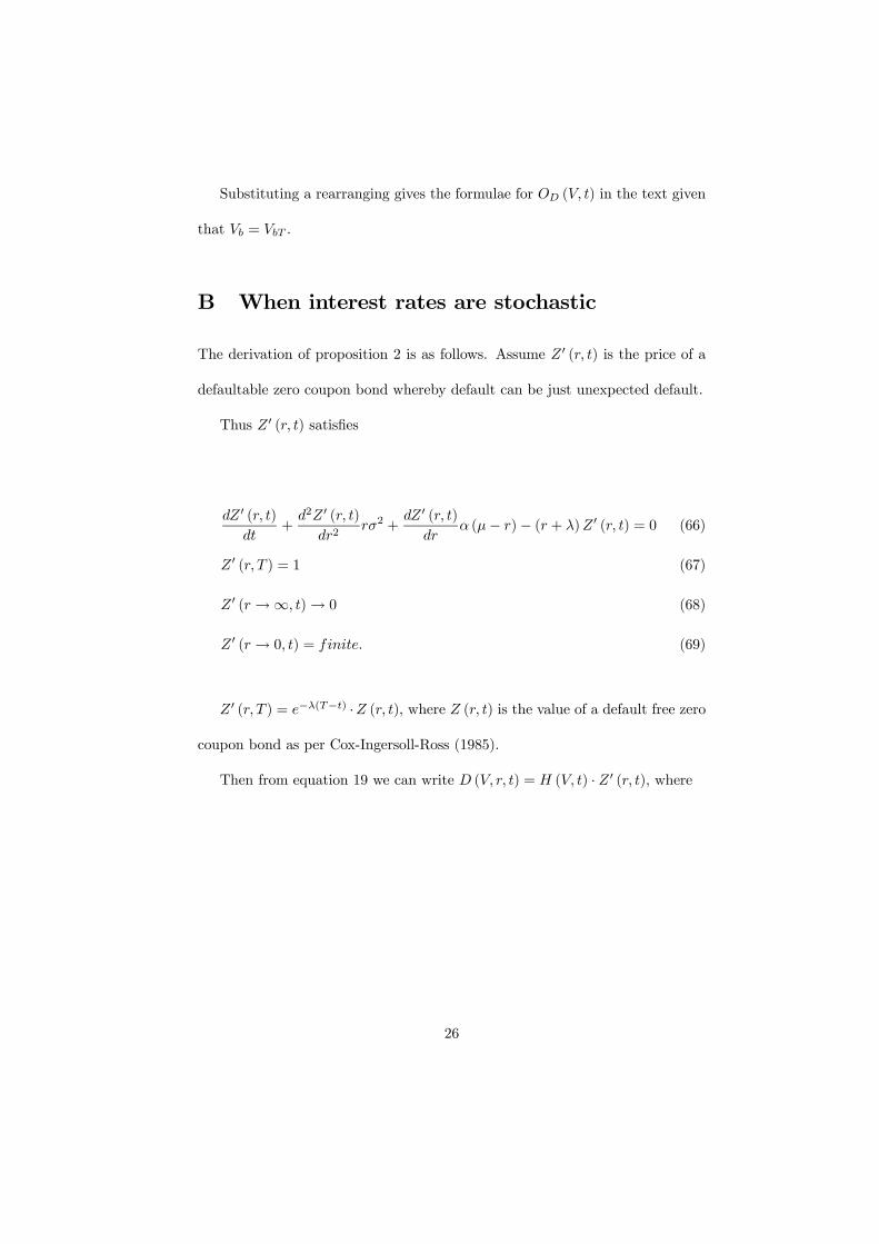
Substituting a rearranging gives the formulae for OD (V, t) in the text given

that Vb = VbT .

B When interest rates are stochastic

The derivation of proposition 2 is as follows. Assume Z0 (r, t) is the price of a

defaultable zero coupon bond whereby default can be just unexpected default.

Thus Z0 (r, t) satisfies

dZ 0 (r, t)dt

+d2Z0 (r, t)

dr2rσ2 +

dZ0 (r, t)dr

α (µ− r)− (r + λ)Z0 (r, t) = 0 (66)

Z0 (r, T ) = 1 (67)

Z0 (r →∞, t)→ 0 (68)

Z0 (r → 0, t) = finite. (69)

Z0 (r, T ) = e−λ(T−t) ·Z (r, t), where Z (r, t) is the value of a default free zero

coupon bond as per Cox-Ingersoll-Ross (1985).

Then from equation 19 we can write D (V, r, t) = H (V, t) · Z 0 (r, t), where

26

dH (V, t)

dt+

d2H (V, t)

dV 2s2V 2 +

dH (V, t)

dV(m− λx · s)V + λ (1− a) = 0 (70)

H (V →∞, r, t)→ 1 (71)

H (Vb, t) = (1− a) (72)

H (V, T ) = 1 (73)

The solution to this partial differential equations for H (V, t) is derived as

follows. First recognise that

H (V, t) = H (V )−O (H (V ) , t) +O1 (V, t) (74)

where H (V ) is such that

d2H (V, t)

dV 2s2V 2 +

dH (V, t)

dV(m− λx · s)V + λ (1− a) = 0 (75)

H (V →∞, r, t)→ 1 (76)

H (Vb, t) = (1− a) (77)

where O (H (V ) , t) is the value of a claim that pays H (V ) at time T if

VT ≥ VbT and if Vt ≥ Vb for any time t < T and that pays nothing otherwise,

and where O1 (V, t) is such that

27

dO1 (V, t)

dt+

d2O1 (V, t)

dV 2s2V 2 +

dO1 (V, t)

dV(m− λx · s)V = 0 (78)

O1 (V →∞, r, t)→ 1 (79)

O1 (Vb, t) = 0 (80)

O1 (V, T ) = 1 (81)

O1 (V, t) is the value of a digital barrier option, whose closed form solution

is well-known and is reported in the text.

Then the solution for H (V ) is

H (V ) =λ (1− a)

r + λ−µλ (1− a)

r + λ

¶µV

Vb

¶qh(82)

qh =− ¡m− λV · s− 1

2s2¢−q¡m− λV · s− 1

2s2¢2+ 2λs2

s2. (83)

Then, from Appendix 1 the value of a claim that pays H (V ) at time T if

VT ≥ VbT and if Vt ≥ Vb for any time t < T and that pays nothing otherwise is:

Q (H (V ) , t, Vb, VbT , T ) = Q

µλ (1− a)

r + λ, t, Vb, VbT , T

¶−Q (A0V q, t, Vb, VbT , T )

with A0 = −λ(1−a)r+λ

1(Vb)

qh , with

28

Q (A0V q, t, Vb, VbT , T ) = A0 · e(−r+nh(qh))(T−t)

·V qhN

µd

µV

VbT, qh

¶¶−µV

Vb

¶−2nh(qh)qh·s2

(Vb)qh ·N

Ãd

Ã(Vb)

2

V · VbT , qh!!

with nh (qh) = (m− λV · s) · qh + 12qh (qh − 1) · s2, with

Q

µλ (1− a)

r + λ, t, Vb, VbT , T

¶=

λ (1− a)

r + λ· e−r(T−t)

·ÃN

µd

µV

VbT, 1

¶− s ·√T − t

¶−µV

Vb

¶1−2 r−bs2

N

Ãd

Ã(Vb)

2

V · VbT , 1!− s ·√T − t

!!

and with Vb = VbT . Substitutions and re-arrangements give the formula for

O (H (V ) , t) in the text.

C When debt recovery value is endogenous

The solution to equation 32 is found as follows. First recognise that

D (V, t) = D (V )−ODh(V, t)−ODl

(V, t) +OP (V, t) (84)

where

D (V ) = Dh (V ) · 1V >Vλ +Dl (V ) · 1V≤Vλ (85)

and Dh (V ) and Dl (V ) are such that

29

d2Dh (V )

dV 2s2V 2 +

dDh (V )

dV(r − b+ λj)V − (r + λ)Dh (V ) + λP + C = 0

(86)

d2Dl (V )

dV 2s2V 2 +

dDl (V )

dV(r − b+ λj)V − (r + λ)Dl (V ) + λ (1− a) (1− j)V + C = 0

(87)

subject to

limV→∞

Dh (V )→ λP

r + λ(88)

Dh (Vλ) = Dl (Vλ, t) (89)·dDh (V )

dV

¸V=Vλ

=

·dDl (V )

dV

¸V=Vλ

(90)

Dl (Vb) = (1− a)Vb (91)

with Vλ =P

(1−j)(1−a) . The solutions to the above ODE’s are:

Dh (V ) =λP + C

r + λ+

µ−λP + C

r + λ+Dl (Vλ, t)

¶µV

Vλ

¶q2(92)

Dl (V ) =λ (1− a) (1− j)V + C

b+ λ+ k1V

q1 + k2Vq2 (93)

with

30

q1,2 =− ¡r − b+ λj − s2

¢±q(r − b+ λj − s2)2 + 4s2 (r + λ)

2s2

k1 =−k2V q2

b + (1− a)Vb − λ(1−a)(1−j)b+λ Vb

V q1b

k2 =

³− λP

r+λ +Dl (Vλ, t)´q2

1Vλ− λ(1−a)(1−j)

b+λ − −k2Vq2b +(1−a)Vb−λ(1−a)(1−j)

b+λ Vb

Vq1b

q1Vq1−1

q2V q2−1 .

Then, the value of a claim that pays min (P, V (1− a)) at time T if Vt ≥ Vb

for any time t < T and that pays nothing otherwise is:

OP (V, t) = P · e−(r+λ)(T−t) · Ωµd

µV

Vb, 1

¶, d

µV 2b

V ·VP , 1¶, 0, 1

¶(94)

+e−λ(T−t) · (1− a) · (95)·Ω

µd

µV

Vb, 1

¶, d

µVbV, 1

¶, 1, 1

¶− Ω

µd

µV

Vb, 1

¶, d

µV 2b

V ·VP , 1¶, 1, 1

¶(96)

Then, the value of a claim that pays Dh (V ) at time T if VT ≥ VP and if

Vt ≥ Vb for any time t < T and that pays nothing otherwise is:

ODh (V, t) =λ+ C

r + λe−(r+λ)(T−t) · Ω

µd−

µV

Vb

¶, d−

µV 2b

V ·Vλ

¶, 0, 1

¶(97)

+

³−λ+C

r+λ +Dl (Vλ, t)´

(Vλ)q2 · e(−(r+λ)+n(q2))(T−t) · Ω

µd

µV

Vb, q2

¶, d

µV 2b

V ·Vλ , q2

¶, q2, q2

¶

Then, the value of a claim that pays Dl (V ) at time T if Vλ ≥ VT ≥ VP and

31

if Vt ≥ Vb for any time t < T and that pays nothing otherwise is:

ODl(V, t) =

C

b+ λe−(r+λ)(T−t) · (98)·

Ω

µd−

µV

Vb

¶, d−

µV 2b

V ·VP

¶, 0, 1

¶− Ω

µd−

µV

Vb

¶, d−

µV 2b

V ·Vλ

¶, 0, 1

¶¸(99)

+λ (1− a) (1− j)

b+ λe−λ(T−t) ··

Ω

µd

µV

Vb, 1

¶, d

µV 2b

V ·VP , 1¶, 1, 1

¶− Ω

µd

µV

Vb, 1

¶, d

µV 2b

V ·Vλ , 1¶, 1, 1

¶¸(100)

+k1 · e(−(r+λ)+n(q1))(T−t) ··Ω

µd

µV

Vb, q1

¶, d

µV 2b

V ·VP , q1

¶, q1, q1

¶− Ω

µd

µV

Vb, q1

¶, d

µV 2b

V ·Vλ , q1

¶, q1, q1

¶¸(101)

+k2 · e(−(r+λ)+n(q2))(T−t) ··Ω

µd

µV

Vb, q2

¶, d

µV 2b

V ·VP , q2

¶, q2, q2

¶− Ω

µd

µV

Vb, q2

¶, d

µV 2b

V ·Vλ , q2

¶, q2, q2

¶¸.(102)

References

[1] Anderson R., and Sundaresan S., 1996, "Design and valuation of debt con-

tracts", Review of financial studies 9, n.1, 37-68.

[2] Black F. and Scholes M., 1973, "The pricing of options and corporate lia-

bilities", Journal of political economy 637-659.

[3] Briys E. and de Varenne F, 1997, Valuing risky fixed rate debt: an exten-

sion, Journal of financial and quantitative analysis 32, n.2, 239-248.

[4] Cathcart L. and El-Jahel Lina, 1998, Valuation of defaultable bonds, Jour-

nal of fixed income, 65-79.

32

[5] Cathcart L. and El-Jahel Lina, 2003, Semianalytical pricing of defaultable

bonds in a signaling jump-default model, Journal of computational finance

6, n.3.

[6] Dufresne P. and Goldstein R., 2001, Do credit spreads reflect stationary

leverage rations?, Journal of Finance 56, 1929 - 1957.

[7] Elton E., Gruber M., Agrawal D. and Mann C., 2001, Explaining the rate

spread on corporate bonds, Journal of Finance 56, 247 - 277.

[8] Ericsson J. and Renault O., 2001, Liquidity and credit risk, EFA 2003.

[9] Ericsson J. and Reneby J., 1998, A framework for pricing corporate secu-

rities, SSE/EFI working paper series in economics and finance n. 314.

[10] Ericsson J. and Reneby J., 1998, On the tradeability of firm’s assets, Work-

ing paper 89 SSE.

[11] Fan H. and Sundaresan S., 2000, "Debt valuation, renegotiation and opti-

mal dividend policy", Review of financial studies 13, n.4, 1057-1099.

[12] Kim J., Ramaswamy K. and Sundaresan S., 1993, "Does default risk in

coupons affect the valuation of corporate bonds?: A contingent claims

model", Financial Management 117-131.

[13] Leland H., 1994a, "Corporate debt value, bond covenants and optimal cap-

ital structure", Journal of finance 49, n.4, 1213-1252.

33

[14] Longstaff F. and Schwartz E., 1995, A simple approach to valuing risky

fixed and floating rate debt, Journal of finance 50, n.3, 789-819.

[15] Mella-Barral P. and Perraudin W., 1997, "Strategic debt service", Journal

of finance 52, n.2, 531-556.

[16] Mella-Barral P. and Tychon P., 1999, "Default Risk in Asset Pricing",

Fothcoming in Finance.

[17] Merton R., 1974, On the pricing of corporate debt: the risk structure of

interest rates, Journal of finance 29, 449-470.

[18] Perraudin W. and Taylor A., 2003, "Liquidity and bond market spreads",

presented at European Finance Association 2003.

[19] Saa-Requejo J. and Santa-Clara P., 1999, Bond pricing with default risk,

Working paper UCLA.

[20] Schlogel L., 1999, A note on the valuation of risky corporate bonds, OR

Spectrum, 35-47.

[21] Tauren M., 1999, A model of corporate bond prices with dynamic capital

structure, Working paper.

[22] Zhou C., 2001, A jump-diffusion approach to modelling credit risk and

valuing defaultable securities, Journal of banking and finance 25, 2015-

2040.

34

0.0%

0.2%

0.4%

0.6%

0.8%

1.0%

1.2%

1.4%

1.6%

0 1 2 3 4 5 6 7 8 9Time to maturity (in years)

Cre

dit s

prea

ds in

per

cent

age

yiel

d

Base caseBase case but λ=1%Base case but V=80, λ=1%

Figure 1:

35

Maturity in years:

(T-t) Base caseBase case but V=90

Base case but V=80

Base case but V=80,

λ=0

Base case but V=80, λ=1%

Base case but V=80, λ=1% and

j=0.6

Base case but V=80, λ=1% and

j=0.50.1 0.06% 0.07% 0.09% 0.00% 0.37% 0.16% 0.00%0.5 0.06% 0.07% 0.09% 0.00% 0.37% 0.16% 0.02%1.0 0.06% 0.07% 0.09% 0.00% 0.37% 0.17% 0.04%1.5 0.06% 0.08% 0.10% 0.01% 0.38% 0.18% 0.06%2.0 0.06% 0.08% 0.12% 0.03% 0.40% 0.20% 0.09%2.5 0.06% 0.09% 0.15% 0.06% 0.43% 0.23% 0.12%3.0 0.06% 0.11% 0.19% 0.10% 0.46% 0.27% 0.16%3.5 0.06% 0.13% 0.23% 0.14% 0.49% 0.30% 0.21%4.0 0.06% 0.14% 0.27% 0.18% 0.53% 0.34% 0.24%4.5 0.06% 0.16% 0.30% 0.21% 0.55% 0.37% 0.28%5.0 0.06% 0.18% 0.33% 0.25% 0.58% 0.40% 0.31%5.5 0.06% 0.20% 0.36% 0.27% 0.60% 0.42% 0.34%6.0 0.06% 0.21% 0.38% 0.30% 0.62% 0.44% 0.36%6.5 0.07% 0.22% 0.40% 0.32% 0.64% 0.46% 0.38%7.0 0.07% 0.23% 0.42% 0.34% 0.65% 0.47% 0.40%7.5 0.08% 0.24% 0.44% 0.36% 0.66% 0.49% 0.42%8.0 0.08% 0.25% 0.45% 0.37% 0.67% 0.50% 0.43%8.5 0.08% 0.26% 0.46% 0.38% 0.68% 0.51% 0.44%9.0 0.09% 0.27% 0.47% 0.39% 0.68% 0.51% 0.45%9.5 0.09% 0.28% 0.48% 0.40% 0.68% 0.52% 0.46%

10.0 0.10% 0.28% 0.48% 0.41% 0.69% 0.52% 0.46%

Table 1

36

Maturity in years:

(T-t) Base caseBase case but V=90

Base case but V=80

Base case but V=80,

s=30%

Base case but V=80, λ=0.5%

Base case but V=80, λ=1%

0.1 0.25% 0.25% 0.25% 0.25% 0.50% 1.00%0.5 0.25% 0.25% 0.25% 0.25% 0.50% 1.00%1.0 0.25% 0.25% 0.25% 0.34% 0.50% 1.00%1.5 0.25% 0.25% 0.26% 0.50% 0.51% 1.01%2.0 0.25% 0.26% 0.28% 0.67% 0.53% 1.02%2.5 0.25% 0.27% 0.31% 0.80% 0.56% 1.05%3.0 0.25% 0.28% 0.34% 0.89% 0.59% 1.09%3.5 0.25% 0.30% 0.38% 0.95% 0.63% 1.12%4.0 0.25% 0.32% 0.42% 0.99% 0.66% 1.15%4.5 0.25% 0.34% 0.45% 1.00% 0.70% 1.18%5.0 0.25% 0.35% 0.49% 1.01% 0.73% 1.21%5.5 0.25% 0.37% 0.51% 1.01% 0.75% 1.23%6.0 0.25% 0.38% 0.54% 1.01% 0.77% 1.25%6.5 0.26% 0.39% 0.56% 1.00% 0.79% 1.27%7.0 0.26% 0.41% 0.57% 0.99% 0.81% 1.28%7.5 0.26% 0.42% 0.59% 0.98% 0.82% 1.29%8.0 0.27% 0.42% 0.60% 0.97% 0.83% 1.30%8.5 0.27% 0.43% 0.61% 0.96% 0.84% 1.30%9.0 0.28% 0.44% 0.62% 0.95% 0.85% 1.31%9.5 0.28% 0.44% 0.63% 0.94% 0.85% 1.31%

10.0 0.28% 0.45% 0.63% 0.93% 0.86% 1.31%

Table 2

37