Embed Size (px)
Citation preview
Direct Yaw Moment Control for Electric
Vehicles with Independent Motors
by
Chunyun Fu
B. Eng.
A thesis submitted in fulfillment of the requirements for the degree of
Doctor of Philosophy (Mechanical and Manufacturing Engineering)
at the
School of Aerospace, Mechanical and Manufacturing Engineering
College of Science, Engineering and Health
RMIT University
August 2014
Declaration of Authorship
I, Chunyun Fu, declare that:
� Except where due acknowledgement has been made, the work is that of the can-
didate alone;
� The work has not been submitted previously, in whole or in part, to qualify for
any other academic award;
� The content of the thesis is the result of work which has been carried out since the
official commencement date of the approved research program;
� Any editorial work, paid or unpaid, carried out by a third party is acknowledged.
Signed:
Date: 25 August 2014
i

Dedicated to my beloved family.
ii
Acknowledgements
I would like to express my very great appreciation to my primary supervisor, Dr. Reza
Hoseinnezhad, for his patient, meticulous and insightful guidance throughout my entire
study.
I would also like to extend my sincere gratitude to Prof. Alireza Bab-Hadiashar, Prof.
Reza N. Jazar and Prof. Simon Watkins for their great advice and assistance during my
research.
My thanks are given to the Formula SAE Tire Test Consortium for providing RMIT
University with tire testing data.
I am particularly grateful for the tremendous support and encouragement from my
parents.
My special thanks go to my beloved fiancee, Faith Luo, for all her love and understand-
ing.
iii
Contents
Declaration of Authorship i
Acknowledgements iii
List of Figures vii
List of Tables x
Abbreviations xi
Publications xiii
Abstract 1
1 Introduction 2
1.1 BACKGROUND AND SCOPE . . . . . . . . . . . . . . . . . . . . . . . . 2
1.1.1 Vehicle stability control . . . . . . . . . . . . . . . . . . . . . . . . 3
1.1.2 Actively controlled mechanical differentials . . . . . . . . . . . . . 4
1.1.3 Direct yaw moment control using independent electric motors . . . 5
1.2 RESEARCH QUESTIONS . . . . . . . . . . . . . . . . . . . . . . . . . . 6
1.2.1 Control variables . . . . . . . . . . . . . . . . . . . . . . . . . . . . 6
1.2.2 Research questions . . . . . . . . . . . . . . . . . . . . . . . . . . . 8
1.3 CONTRIBUTIONS . . . . . . . . . . . . . . . . . . . . . . . . . . . . . . 9
1.4 THESIS OUTLINE . . . . . . . . . . . . . . . . . . . . . . . . . . . . . . . 9
2 Literature Review 11
2.1 EQUAL TORQUE METHODS . . . . . . . . . . . . . . . . . . . . . . . . 11
2.2 ACKERMAN METHODS . . . . . . . . . . . . . . . . . . . . . . . . . . . 13
2.2.1 Background . . . . . . . . . . . . . . . . . . . . . . . . . . . . . . . 13
2.2.2 Control methods based on Ackerman steering geometry . . . . . . 15
2.2.3 Remarks . . . . . . . . . . . . . . . . . . . . . . . . . . . . . . . . . 17
2.3 YAW RATE-BASED DYC . . . . . . . . . . . . . . . . . . . . . . . . . . 18
2.3.1 Background . . . . . . . . . . . . . . . . . . . . . . . . . . . . . . . 18
2.3.2 Typical yaw rate-based DYC methods . . . . . . . . . . . . . . . . 20
2.3.3 Remarks . . . . . . . . . . . . . . . . . . . . . . . . . . . . . . . . . 25
iv
Contents v
2.4 VEHICLE SIDE-SLIP-BASED DYC . . . . . . . . . . . . . . . . . . . . . 26
2.4.1 Background . . . . . . . . . . . . . . . . . . . . . . . . . . . . . . . 26
2.4.2 Typical vehicle side-slip-based DYC methods . . . . . . . . . . . . 27
2.4.3 Remarks . . . . . . . . . . . . . . . . . . . . . . . . . . . . . . . . . 29
2.5 SIMULTANEOUS CONTROL OF YAW RATE AND VEHICLE SIDE-SLIP . . . . . . . . . . . . . . . . . . . . . . . . . . . . . . . . . . . . . . . 30
2.5.1 Background . . . . . . . . . . . . . . . . . . . . . . . . . . . . . . . 30
2.5.2 Typical control methods . . . . . . . . . . . . . . . . . . . . . . . . 30
2.5.3 Remarks . . . . . . . . . . . . . . . . . . . . . . . . . . . . . . . . . 35
3 Full Vehicle Model 37
3.1 VEHICLE EQUIVALENT MECHANICAL MODEL . . . . . . . . . . . . 37
3.2 VEHICLE EQUATIONS OF MOTION . . . . . . . . . . . . . . . . . . . 38
3.2.1 Translational motion . . . . . . . . . . . . . . . . . . . . . . . . . . 39
3.2.2 Rotational motion . . . . . . . . . . . . . . . . . . . . . . . . . . . 44
3.3 WHEEL EQUATION OF MOTION . . . . . . . . . . . . . . . . . . . . . 49
3.4 TIRE MODEL . . . . . . . . . . . . . . . . . . . . . . . . . . . . . . . . . 50
4 Yaw Rate-Based Direct Yaw Moment Control 55
4.1 BACKGROUND . . . . . . . . . . . . . . . . . . . . . . . . . . . . . . . . 55
4.2 VEHICLE CONTROL MODEL DERIVATION . . . . . . . . . . . . . . . 57
4.3 YAW RATE-BASED DYC DESIGN . . . . . . . . . . . . . . . . . . . . . 60
4.4 SIMULATION RESULTS . . . . . . . . . . . . . . . . . . . . . . . . . . . 65
4.4.1 Simulations with step inputs . . . . . . . . . . . . . . . . . . . . . 66
4.4.1.1 Step input δ = 0.1 rad . . . . . . . . . . . . . . . . . . . . 67
4.4.1.2 Step inputs δ = 0.075 rad and δ = 0.05 rad . . . . . . . . 70
4.4.2 Simulations with sinusoidal inputs . . . . . . . . . . . . . . . . . . 71
4.5 SUMMARY . . . . . . . . . . . . . . . . . . . . . . . . . . . . . . . . . . . 72
5 Vehicle Side-Slip-Based Direct Yaw Moment Control 75
5.1 BACKGROUND . . . . . . . . . . . . . . . . . . . . . . . . . . . . . . . . 75
5.2 VEHICLE SIDE-SLIP-BASED DYC DESIGN . . . . . . . . . . . . . . . 76
5.2.1 Controller design . . . . . . . . . . . . . . . . . . . . . . . . . . . . 76
5.2.2 Controller effect on yaw rate . . . . . . . . . . . . . . . . . . . . . 78
5.2.3 Complete control structure . . . . . . . . . . . . . . . . . . . . . . 79
5.3 SIMULATION RESULTS . . . . . . . . . . . . . . . . . . . . . . . . . . . 79
5.3.1 Simulations with step inputs . . . . . . . . . . . . . . . . . . . . . 80
5.3.2 Simulations with sinusoidal inputs . . . . . . . . . . . . . . . . . . 86
5.4 SUMMARY . . . . . . . . . . . . . . . . . . . . . . . . . . . . . . . . . . . 89
6 Simultaneous Control of Yaw Rate and Vehicle Side-Slip 90
6.1 BACKGROUND . . . . . . . . . . . . . . . . . . . . . . . . . . . . . . . . 90
6.2 PROPOSED DYC DESIGN . . . . . . . . . . . . . . . . . . . . . . . . . . 92
6.3 SIMULATION RESULTS . . . . . . . . . . . . . . . . . . . . . . . . . . . 96
6.3.1 Simulations with constant vx . . . . . . . . . . . . . . . . . . . . . 97
6.3.1.1 J-turn and lane change maneuvers at vx = 60 km/h . . . 97
6.3.1.2 J-turn and lane change maneuvers at vx = 80 km/h . . . 106
6.3.2 Simulations with uncontrolled vx . . . . . . . . . . . . . . . . . . . 113
Contents vi
6.3.2.1 J-turn and lane change maneuvers starting at vx = 60km/h . . . . . . . . . . . . . . . . . . . . . . . . . . . . . 113
6.3.2.2 J-turn and lane change maneuvers starting at vx = 80km/h . . . . . . . . . . . . . . . . . . . . . . . . . . . . . 123
6.4 SUMMARY . . . . . . . . . . . . . . . . . . . . . . . . . . . . . . . . . . . 133
7 Conclusions and Recommendations 134
7.1 CONCLUSIONS . . . . . . . . . . . . . . . . . . . . . . . . . . . . . . . . 134
7.2 RECOMMENDATIONS . . . . . . . . . . . . . . . . . . . . . . . . . . . . 136
Appendix 138
Bibliography 149
List of Figures
1.1 Bosch ESP system. . . . . . . . . . . . . . . . . . . . . . . . . . . . . . . . 3
1.2 Schematic of an example rear active differential. . . . . . . . . . . . . . . 4
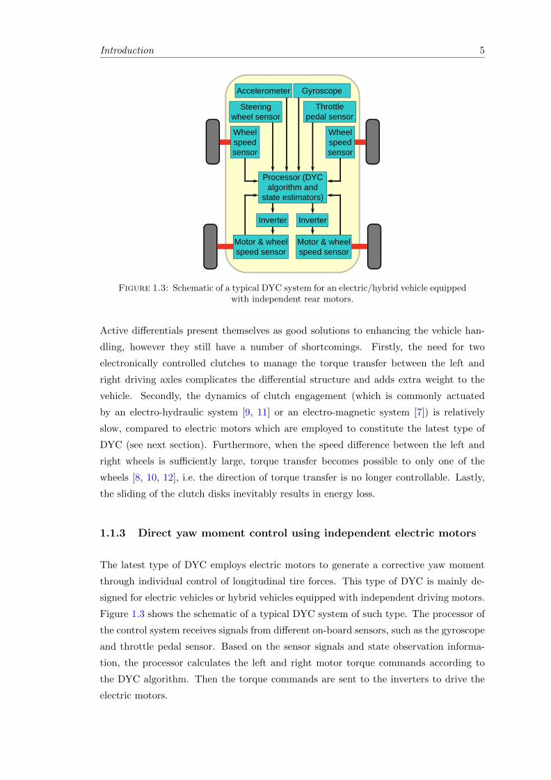
1.3 Schematic of a typical DYC system for an electric/hybrid vehicle equippedwith independent rear motors. . . . . . . . . . . . . . . . . . . . . . . . . . 5
1.4 Vehicle top view. . . . . . . . . . . . . . . . . . . . . . . . . . . . . . . . . 7
2.1 An example equal torque method. . . . . . . . . . . . . . . . . . . . . . . 12
2.2 An example equal torque method with self-blocking control. . . . . . . . . 13
2.3 Ackerman steering geometry. . . . . . . . . . . . . . . . . . . . . . . . . . 14
2.4 Electric vehicle configuration proposed by Cordeiro et al. . . . . . . . . . 15
2.5 Electrical drive proposed by Cordeiro et al. . . . . . . . . . . . . . . . . . 16
2.6 Schematic of electrical differential system proposed by Haddoun et al. . . 16
2.7 Schematic of torque split control proposed by Doniselli et al. . . . . . . . 21
2.8 Schematic of DYC proposed by Hancock et al. . . . . . . . . . . . . . . . 24
2.9 Schematic of DYC proposed by lkushima and Sawase. . . . . . . . . . . . 25
2.10 Schematic of the hybrid power-train. . . . . . . . . . . . . . . . . . . . . . 33
3.1 Vehicle equivalent mechanical model and vehicle coordinate systems. . . . 38
3.2 Description of rigid body general motion. . . . . . . . . . . . . . . . . . . 39
3.3 Wheel schematic. . . . . . . . . . . . . . . . . . . . . . . . . . . . . . . . . 50
3.4 Schematic of the vehicle longitudinal motion. . . . . . . . . . . . . . . . . 52
3.5 Front view of the vehicle equivalent mechanical model. . . . . . . . . . . . 53
4.1 Force system acting on the vehicle. . . . . . . . . . . . . . . . . . . . . . . 61
4.2 Schematic of the proposed DYC system. . . . . . . . . . . . . . . . . . . . 64
4.3 Third generation all-electric racing car developed at RMIT University. . . 65
4.4 Yaw rate error responses to the step input δ = 0.1 rad. . . . . . . . . . . . 67
4.5 Vehicle path responses to the step input δ = 0.1 rad during the first 12.5 sof simulation. . . . . . . . . . . . . . . . . . . . . . . . . . . . . . . . . . . 68
4.6 Wheel slip ratio responses of the inner driving wheel to the step inputδ = 0.1 rad. . . . . . . . . . . . . . . . . . . . . . . . . . . . . . . . . . . . 68
4.7 Longitudinal tire force responses of the inner driving wheel to step inputδ = 0.1 rad. . . . . . . . . . . . . . . . . . . . . . . . . . . . . . . . . . . . 69
4.8 Wheel angular velocity responses of the two driving wheels to the stepinput δ = 0.1 rad using the proposed DYC. . . . . . . . . . . . . . . . . . 69
4.9 Yaw rate error responses to the step input δ = 0.075 rad. . . . . . . . . . 70
4.10 Vehicle path responses to the step input δ = 0.075 rad during the first13.5 s of simulation. . . . . . . . . . . . . . . . . . . . . . . . . . . . . . . 70
4.11 Yaw rate error responses to the step input δ = 0.05 rad. . . . . . . . . . . 71
vii
List of Figures viii
4.12 Vehicle path responses to the step input δ = 0.05 rad during the first 15 sof simulation. . . . . . . . . . . . . . . . . . . . . . . . . . . . . . . . . . . 71
4.13 Yaw rate error responses to the sinusoidal input δ = 0.1 sinπt rad. . . . . 72
4.14 Yaw rate error responses to the sinusoidal input δ = 0.1 sin 0.5πt rad. . . . 73
4.15 Yaw rate error responses to the sinusoidal input δ = 0.05 sinπt rad. . . . . 73
4.16 Yaw rate error responses to the sinusoidal input δ = 0.05 sin 0.5πt rad. . . 73
5.1 Schematic of the proposed DYC system. . . . . . . . . . . . . . . . . . . . 80
5.2 Vehicle side-slip responses to the step input δ = 0.1 rad. . . . . . . . . . . 81
5.3 Yaw rate responses to the step input δ = 0.1 rad. . . . . . . . . . . . . . . 82
5.4 Wheel slip ratio responses of the inner-driving wheel to the step inputδ = 0.1 rad. . . . . . . . . . . . . . . . . . . . . . . . . . . . . . . . . . . . 83
5.5 Longitudinal tire force responses of the inner-driving wheel to the stepinput δ = 0.1 rad. . . . . . . . . . . . . . . . . . . . . . . . . . . . . . . . . 83
5.6 Wheel angular velocity responses of the two driving wheels to the stepinput δ = 0.1 rad using the proposed DYC. . . . . . . . . . . . . . . . . . 84
5.7 Vehicle side-slip responses to the step input δ = 0.12 rad. . . . . . . . . . 84
5.8 Yaw rate responses to the step input δ = 0.12 rad. . . . . . . . . . . . . . 85
5.9 Wheel slip ratio responses of the inner-driving wheel to the step inputδ = 0.12 rad. . . . . . . . . . . . . . . . . . . . . . . . . . . . . . . . . . . 85
5.10 Vehicle side-slip responses to the sinusoidal input δ = 0.1 sinπ
3t rad. . . . 86
5.11 Yaw rate responses to the sinusoidal input δ = 0.1 sinπ
3t rad. . . . . . . . 87
5.12 Wheel slip ratio responses of the inner-driving wheel to the sinusoidal
input δ = 0.1 sinπ
3t rad. . . . . . . . . . . . . . . . . . . . . . . . . . . . . 87
5.13 Vehicle side-slip responses to the sinusoidal input δ = 0.13 sinπ
3t rad. . . . 88
5.14 Yaw rate responses to the sinusoidal input δ = 0.13 sinπ
3t rad. . . . . . . . 88
5.15 Wheel slip ratio responses of the inner-driving wheel to the sinusoidal
input δ = 0.13 sinπ
3t rad. . . . . . . . . . . . . . . . . . . . . . . . . . . . 89
6.1 Schematic of the proposed DYC system. . . . . . . . . . . . . . . . . . . . 96
6.2 Front wheel steer angle for the J-turn maneuver at vx = 60 km/h. . . . . 98
6.3 Yaw rate responses of the J-turn maneuver when vx = 60 km/h and (a)ρ = 0.75 (b) ρ = 0.5 (c) ρ = 0.25. . . . . . . . . . . . . . . . . . . . . . . . 99
6.4 Vehicle paths of the J-turn maneuver when vx = 60 km/h and (a) ρ = 0.75(b) ρ = 0.5 (c) ρ = 0.25. . . . . . . . . . . . . . . . . . . . . . . . . . . . . 100
6.5 Vehicle side-slip responses of the J-turn maneuver when vx = 60 km/hand (a) ρ = 0.75 (b) ρ = 0.5 (c) ρ = 0.25. . . . . . . . . . . . . . . . . . . 101
6.6 Front wheel steer angle for the lane change maneuver at vx = 60 km/h. . 102
6.7 Yaw rate responses of the lane change maneuver when vx = 60 km/h and(a) ρ = 0.75 (b) ρ = 0.5 (c) ρ = 0.25. . . . . . . . . . . . . . . . . . . . . . 103
6.8 Vehicle paths of the lane change maneuver when vx = 60 km/h and (a)ρ = 0.75 (b) ρ = 0.5 (c) ρ = 0.25. . . . . . . . . . . . . . . . . . . . . . . . 104
6.9 Vehicle side-slip responses of the lane change maneuver when vx = 60 km/hand (a) ρ = 0.75 (b) ρ = 0.5 (c) ρ = 0.25. . . . . . . . . . . . . . . . . . . 105
6.10 Front wheel steer angle for the J-turn maneuver at vx = 80 km/h. . . . . 107
List of Figures ix
6.11 Yaw rate responses of the J-turn maneuver when vx = 80 km/h and (a)ρ = 0.75 (b) ρ = 0.5 (c) ρ = 0.25. . . . . . . . . . . . . . . . . . . . . . . . 107
6.12 Vehicle paths of the J-turn maneuver when vx = 80 km/h and (a) ρ = 0.75(b) ρ = 0.5 (c) ρ = 0.25. . . . . . . . . . . . . . . . . . . . . . . . . . . . . 108
6.13 Vehicle side-slip responses of the J-turn maneuver when vx = 80 km/hand (a) ρ = 0.75 (b) ρ = 0.5 (c) ρ = 0.25. . . . . . . . . . . . . . . . . . . 109
6.14 Front wheel steer angle for the lane change maneuver at vx = 80 km/h. . 110
6.15 Yaw rate responses of the lane change maneuver when vx = 80 km/h and(a) ρ = 0.75 (b) ρ = 0.5 (c) ρ = 0.25. . . . . . . . . . . . . . . . . . . . . . 110
6.16 Vehicle paths of the lane change maneuver when vx = 80 km/h and (a)ρ = 0.75 (b) ρ = 0.5 (c) ρ = 0.25. . . . . . . . . . . . . . . . . . . . . . . . 111
6.17 Vehicle side-slip responses of the lane change maneuver when vx = 80 km/hand (a) ρ = 0.75 (b) ρ = 0.5 (c) ρ = 0.25. . . . . . . . . . . . . . . . . . . 112
6.18 Vehicle longitudinal velocity responses of the J-turn maneuver starting atvx = 60 km/h with (a) ρ = 0.75 (b) ρ = 0.5 (c) ρ = 0.25. . . . . . . . . . . 114
6.19 Yaw rate responses of the J-turn maneuver starting at vx = 60 km/h with(a) ρ = 0.75 (b) ρ = 0.5 (c) ρ = 0.25. . . . . . . . . . . . . . . . . . . . . . 115
6.20 Vehicle paths of the J-turn maneuver starting at vx = 60 km/h with (a)ρ = 0.75 (b) ρ = 0.5 (c) ρ = 0.25. . . . . . . . . . . . . . . . . . . . . . . . 116
6.21 Vehicle side-slip responses of the J-turn maneuver starting at vx = 60 km/hwith (a) ρ = 0.75 (b) ρ = 0.5 (c) ρ = 0.25. . . . . . . . . . . . . . . . . . . 117
6.22 Vehicle longitudinal velocity responses of the lane change maneuver start-ing at vx = 60 km/h with (a) ρ = 0.75 (b) ρ = 0.5 (c) ρ = 0.25. . . . . . . 119
6.23 Yaw rate responses of the lane change maneuver starting at vx = 60 km/hwith (a) ρ = 0.75 (b) ρ = 0.5 (c) ρ = 0.25. . . . . . . . . . . . . . . . . . . 120
6.24 Vehicle paths of the lane change maneuver starting at vx = 60 km/h with(a) ρ = 0.75 (b) ρ = 0.5 (c) ρ = 0.25. . . . . . . . . . . . . . . . . . . . . . 121
6.25 Vehicle side-slip responses of the lane change maneuver starting at vx =60 km/h with (a) ρ = 0.75 (b) ρ = 0.5 (c) ρ = 0.25. . . . . . . . . . . . . . 122
6.26 Vehicle longitudinal velocity responses of the J-turn maneuver starting atvx = 80 km/h with (a) ρ = 0.75 (b) ρ = 0.5 (c) ρ = 0.25. . . . . . . . . . . 124
6.27 Yaw rate responses of the J-turn maneuver starting at vx = 80 km/h with(a) ρ = 0.75 (b) ρ = 0.5 (c) ρ = 0.25. . . . . . . . . . . . . . . . . . . . . . 125
6.28 Vehicle paths of the J-turn maneuver starting at vx = 80 km/h with (a)ρ = 0.75 (b) ρ = 0.5 (c) ρ = 0.25. . . . . . . . . . . . . . . . . . . . . . . . 126
6.29 Vehicle side-slip responses of the J-turn maneuver starting at vx = 80 km/hwith (a) ρ = 0.75 (b) ρ = 0.5 (c) ρ = 0.25. . . . . . . . . . . . . . . . . . . 127
6.30 Vehicle longitudinal velocity responses of the lane change maneuver start-ing at vx = 80 km/h with (a) ρ = 0.75 (b) ρ = 0.5 (c) ρ = 0.25. . . . . . . 129
6.31 Yaw rate responses of the lane change maneuver starting at vx = 80 km/hwith (a) ρ = 0.75 (b) ρ = 0.5 (c) ρ = 0.25. . . . . . . . . . . . . . . . . . . 130
6.32 Vehicle paths of the lane change maneuver starting at vx = 80 km/h with(a) ρ = 0.75 (b) ρ = 0.5 (c) ρ = 0.25. . . . . . . . . . . . . . . . . . . . . . 131
6.33 Vehicle side-slip responses of the lane change maneuver starting at vx =80 km/h with (a) ρ = 0.75 (b) ρ = 0.5 (c) ρ = 0.25. . . . . . . . . . . . . . 132
List of Tables
4.1 Vehicle parameters of the electric racing car. . . . . . . . . . . . . . . . . 66
5.1 Average errors of the vehicle side-slip and yaw rate. . . . . . . . . . . . . 86
x
Abbreviations
2WD 2-Wheel-Drive
2WS 2-Wheel-Steering
4WD 4-Wheel-Drive
4WS 4-Wheel-Steering
ABS Anti-lock Braking System
AFS Active Front-wheel Steering
ARCS Active Roll Control System
CVT Continuously Variable Transmission
DoF Degree-of-Freedom
DYC Direct Yaw-moment Control
ECU Electronic Control Unit
ESC Electronic Stability Control
ESP Electronic Stability Program
HEV Hybrid Electric Vehicle
HIL Hardware-In-the-Loop
I Integral
ICC Integrated Chassis Control
ICE Internal Combustion Engine
LQR Linear Quadratic Regulator
LSD Limited Slip Differential
MRAS Model Reference Adaptive System
PD Proportional-Derivative
PI Proportional-Integral
PID Proportional-Integral-Derivative
PMBDCM Permanent Magnet Brushless Direct Current Motor
xi
Abbreviations xii
RNN Recurrent Neural Network
SMO Sliding Mode Observer
TCS Traction Control System
TTC Tire Test Consortium
VDC Vehicle Dynamics Control
VSC Vehicle Stability Control
WLS Weighted Least Square
Publications
CONFERENCE PAPERS
• C. Fu, R. Hoseinnezhad, S. Watkins, and R. N. Jazar, “Direct torque control
for electronic differential in an electric racing car,” in Proceedings - 4th Inter-
national Conference on Sustainable Automotive Technologies, ICSAT 2012, Mel-
bourne, Australia, 2012, pp. 177-183.
• C. Fu, R. Hoseinnezhad, R. N. Jazar, A. Bab-Hadiashar, and S. Watkins, “Elec-
tronic differential design for vehicle side-slip control,” in Proceedings - 2012 Inter-
national Conference on Control, Automation and Information Sciences, ICCAIS
2012, Ho Chi Minh City, Vietnam, 2012, pp. 306-310.
JOURNAL PAPERS
• C. Fu, R. Hoseinnezhad, and A. Bab-Hadiashar, “Side-slip control for nonlinear
vehicle dynamics by electronic differentials,” Nonlinear Engineering, vol. 1, no.
1-2, pp. 1-10, 2012.
• C. Fu, R. Hoseinnezhad, A. Bab-Hadiashar, R. N. Jazar, and S. Watkins, “Elec-
tronic differential for high-performance electric vehicles with independent driving
motors,” International Journal of Electric and Hybrid Vehicles, vol. 6, no. 2, pp.
108-132, 2014.
• M. Hu, H. Xie, and C. Fu, “Study on EV transmission system parameter design
based on vehicle dynamic performance,” International Journal of Electric and
Hybrid Vehicles, vol. 6, no. 2, pp. 133-151, 2014.
xiii
Publications xiv
• C. Fu, R. Hoseinnezhad, A. Bab-Hadiashar, and R. N. Jazar, “Direct yaw moment
control for electric and hybrid vehicles with independent motors,” International
Journal of Vehicle Design, accepted.
• M. Hu, J. Zeng, S. Xu, C. Fu, and D. Qin “Efficiency study of a dual-motor
coupling EV powertrain,” IEEE Transactions on Vehicular Technology, accepted,
doi: 10.1109/TVT.2014.2347349.
• C. Fu, R. Hoseinnezhad, A. Bab-Hadiashar, and R. N. Jazar, “Electric vehicle
side-slip control via electronic differential,” submitted to International Journal of
Vehicle Autonomous Systems.
Abstract
Direct Yaw Moment Control (DYC) systems generate a corrective yaw moment to alter
the vehicle dynamics by means of active distribution of the longitudinal tire forces,
and they have been proven to be an effective means to enhance the vehicle handling
and stability. The latest type of DYC systems employs the on-board electric motors of
electric or hybrid vehicles to generate the corrective yaw moment, and it has presented
itself as a more effective approach than the conventional DYC schemes.
In this thesis, a wide range of existing vehicle dynamics control designs, especially the
typical DYC solutions, are investigated. The theories and principles behind these control
methods are summarized, and the features of each control scheme are highlighted. Then,
a full vehicle model including the vehicle equivalent mechanical model, vehicle equations
of motion, wheel equation of motion and Magic Formula tire model is established.
Using the derived vehicle equations of motion, the fundamental mathematical relation-
ships between the corrective yaw moment produced by the DYC system and the crucial
vehicle states (the yaw rate and vehicle side-slip) are derived. Based on these relation-
ships, two DYC systems are proposed for electric vehicles (or hybrid vehicles) by means
of individual control of the independent driving motors. These two systems are designed
to track the desired yaw rate and vehicle side-slip, respectively. Extensive simulation
results verify that these systems are effective in improving vehicle dynamic performance.
Apart from the two systems that adjust yaw rate or vehicle side-slip individually, a novel
sliding mode DYC scheme is proposed to regulate both vehicle states simultaneously,
aiming to better enhance the vehicle handling and stability. This control scheme guar-
antees the simultaneous convergences of both the yaw rate and vehicle side-slip errors
to zero, and eliminates the limitations presented in the common sliding mode DYC
solutions. Comparative simulation results indicate that the vehicle handling and sta-
bility are significantly enhanced with the proposed DYC system on-board. Also, this
DYC scheme is shown to outperform its corresponding counterparts in various driving
conditions.
1
Chapter 1
Introduction
1.1 BACKGROUND AND SCOPE
Not long ago, restricted by the control techniques of the day, the braking torques gen-
erated by a vehicle braking system were evenly distributed between the left and right
wheels. Also, the driving torque produced by an Internal Combustion Engine (ICE) was
transferred equally to the left and right driving wheels, or mechanically altered between
the left and right wheels using, for example, a Torsen differential. As a result, the lon-
gitudinal tire forces (braking or traction forces) were not utilized to actively generate
yaw moments to regulate the vehicle motions. Yaw moments were, at large, generated
by the lateral tire forces through tire slip angles during steering motions.
The lack of control on yaw moment has brought about some problems. In some critical
driving scenarios (e.g. the vehicle enters a road with uneven surface conditions or the
vehicle corners sharply at a high speed), the yaw moment that is naturally generated by
the lateral tire forces may be excessive or insufficient to keep the vehicle stable, and can
result in accidents. On the other hand, passenger cars are normally designed to have
understeer characteristic to gain more stability margin. Note that the level of understeer
varies as the driving condition changes. For example, if the lateral load transfer of the
front wheels is greater than that of the rear wheels, then the level of understeer intensifies;
otherwise the level of understeer attenuates. In extreme cases, the lateral load transfer
can even force the vehicle to switch from understeer to oversteer. A conventional vehicle
cannot consistently remain in a desirable steer characteristic, say, neutral steer.
In view of the above problems, several types of electronic control systems have been
proposed in the last three decades, aiming to regulate the vehicle yaw motion by means
of active distribution of longitudinal tire forces (both braking and traction forces). A
2
Introduction 3
(a) ESP configuration (b) ESP components
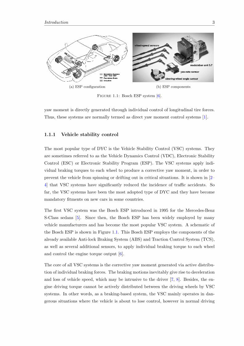
Figure 1.1: Bosch ESP system [6].
yaw moment is directly generated through individual control of longitudinal tire forces.
Thus, these systems are normally termed as direct yaw moment control systems [1].
1.1.1 Vehicle stability control
The most popular type of DYC is the Vehicle Stability Control (VSC) systems. They
are sometimes referred to as the Vehicle Dynamics Control (VDC), Electronic Stability
Control (ESC) or Electronic Stability Program (ESP). The VSC systems apply indi-
vidual braking torques to each wheel to produce a corrective yaw moment, in order to
prevent the vehicle from spinning or drifting out in critical situations. It is shown in [2–
4] that VSC systems have significantly reduced the incidence of traffic accidents. So
far, the VSC systems have been the most adopted type of DYC and they have become
mandatory fitments on new cars in some countries.
The first VSC system was the Bosch ESP introduced in 1995 for the Mercedes-Benz
S-Class sedans [5]. Since then, the Bosch ESP has been widely employed by many
vehicle manufacturers and has become the most popular VSC system. A schematic of
the Bosch ESP is shown in Figure 1.1. This Bosch ESP employs the components of the
already available Anti-lock Braking System (ABS) and Traction Control System (TCS),
as well as several additional sensors, to apply individual braking torque to each wheel
and control the engine torque output [6].
The core of all VSC systems is the corrective yaw moment generated via active distribu-
tion of individual braking forces. The braking motions inevitably give rise to deceleration
and loss of vehicle speed, which may be intrusive to the driver [7, 8]. Besides, the en-
gine driving torque cannot be actively distributed between the driving wheels by VSC
systems. In other words, as a braking-based system, the VSC mainly operates in dan-
gerous situations where the vehicle is about to lose control, however in normal driving
Introduction 4CANALE et al.: VEHICLE YAW CONTROL VIA SECOND-ORDER SLIDING-MODE TECHNIQUE 3909
Fig. 1. (Dotted) Uncontrolled vehicle and (solid) target steering diagrams.Vehicle speed: 100 km/h.
II. PROBLEM FORMULATION AND
CONTROL REQUIREMENTS
The first control objective of any active stability system isto improve safety in critical maneuvers and in the presenceof unusual external conditions, such as strong lateral wind orchanging road friction coefficient. Moreover, the consideredRAD device can be employed to change the steady-state anddynamic behavior of the car, improving its handling properties.The vehicle inputs are the steering angle δ, commanded bythe driver, and the external forces and moments applied to thevehicle center of gravity. The most significant variables de-scribing the behavior of the vehicle are its speed v(t), lateralacceleration ay(t), yaw rate ψ(t), and side slip angle β(t). Re-garding the vehicle as a rigid body moving at constant speed v,the following relationship between ay(t), ψ(t), and β(t) holds:
ay(t) = v(ψ(t) + β(t)
). (1)
In steady-state motion β(t) = 0, the lateral acceleration is pro-portional to yaw rate through the vehicle speed. In this situation,let us consider the uncontrolled car behavior: For each constantspeed value, by means of standard steering pad maneuvers,it is possible to obtain the steady-state lateral acceleration ay
corresponding to different values of the steering angle δ. Thesevalues can be graphically represented on the so-called steeringdiagram (see Fig. 1, dotted line). Such curves are mostly influ-enced by road friction and depend on the tire lateral force–slipcharacteristics. At low acceleration, the shape of the steeringdiagram is linear and its slope is a measure of the readiness ofthe car: the lower this value, the higher the lateral accelerationreached by the vehicle with the same steering angle and thebetter the maneuverability and handling quality perceived bythe driver [21]. At high lateral acceleration, the behavior be-comes nonlinear, showing a saturation value that is the highestlateral acceleration the vehicle can reach. The intervention of anactive differential device can be considered as a yaw momentMz(t) acting on the car center of gravity: Such a moment iscapable of changing, under the same steering conditions, the
Fig. 2. RAD schematic. The input shaft 1 transfers driving power to thetraditional bevel gear differential 2 and, through the additional gearing 3, tothe clutch housings 4. Clutch disks 5 are fixed to the output axles 6.
behavior of ay , modifying the steering diagram according tosome desired requirements. Thus, a target steering diagram (asshown in Fig. 1, solid line) can be introduced to take intoaccount the performance improvements to be obtained by thecontrol system. More details about the generation of such targetsteering diagrams are reported in Section IV-A. Therefore, thechoice of yaw rate ψ as the controlled variable is fully justified,also considering its reliability and ease of measurement on thecar. A reference generator will provide the desired values ψref
for the yaw rate ψ needed to achieve the desired performancesby means of a suitably designed feedback control law.
As for the generation of the required yaw moment Mz(t), inthis paper, a full RAD is considered (see [9]–[14] for details).A schematic of the RAD taken into account in this paper isshown in Fig. 2. This device is basically a traditional bevel geardifferential that has been modified in order to transfer motion totwo clutch housings, which rotate together with the input gear.Clutch friction disks are fixed on each differential output axle.The ratio between the input angular speed of the differential andthe angular speeds of the clutch housings is such that the latterrotate faster than their respective disks in almost every vehiclemotion condition (i.e., except for narrow cornering at very lowvehicle speed); thus, the sign of each clutch torque is alwaysknown, and the torque magnitude only depends on the clutchactuation force, which is generated by an electrohydraulicsystem whose input current is determined by the controller. Themain advantage of this system is the capability of generatingthe yaw moment of every value within the actuation systemsaturation limits, regardless of the input driving torque valueand the speed values of the rear wheels. The considered devicehas a yaw moment saturation value of ±2500 N · m, due to thephysical limits of its electrohydraulic system.
The actuator dynamics can be described by the followingfirst-order model [5]:
GA(s) =Mz(s)
IM (s)=
KA
1 + s/ωA(2)
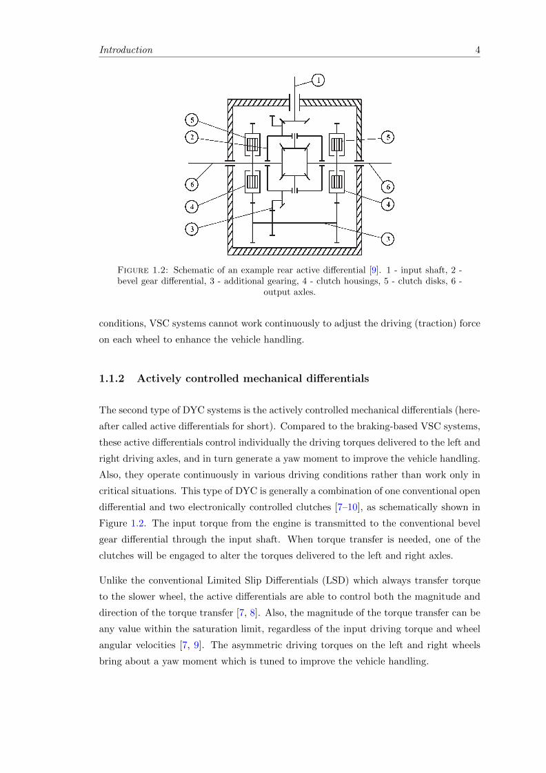
Figure 1.2: Schematic of an example rear active differential [9]. 1 - input shaft, 2 -bevel gear differential, 3 - additional gearing, 4 - clutch housings, 5 - clutch disks, 6 -
output axles.
conditions, VSC systems cannot work continuously to adjust the driving (traction) force
on each wheel to enhance the vehicle handling.
1.1.2 Actively controlled mechanical differentials
The second type of DYC systems is the actively controlled mechanical differentials (here-
after called active differentials for short). Compared to the braking-based VSC systems,
these active differentials control individually the driving torques delivered to the left and
right driving axles, and in turn generate a yaw moment to improve the vehicle handling.
Also, they operate continuously in various driving conditions rather than work only in
critical situations. This type of DYC is generally a combination of one conventional open
differential and two electronically controlled clutches [7–10], as schematically shown in
Figure 1.2. The input torque from the engine is transmitted to the conventional bevel
gear differential through the input shaft. When torque transfer is needed, one of the
clutches will be engaged to alter the torques delivered to the left and right axles.
Unlike the conventional Limited Slip Differentials (LSD) which always transfer torque
to the slower wheel, the active differentials are able to control both the magnitude and
direction of the torque transfer [7, 8]. Also, the magnitude of the torque transfer can be
any value within the saturation limit, regardless of the input driving torque and wheel
angular velocities [7, 9]. The asymmetric driving torques on the left and right wheels
bring about a yaw moment which is tuned to improve the vehicle handling.
Introduction 5
RMIT University©2014 Science, Engineering & Health 8
Background
An example DYC system for an electric/hybrid vehicle equipped with independent rear motors.
Motor & wheel speed sensor
Inverter
Processor (DYC algorithm and
state estimators)
Accelerometer
Motor & wheel speed sensor
Steering wheel sensor
Inverter
Throttle pedal sensor
Gyroscope
Wheel speed sensor
Wheel speed sensor
Figure 1.3: Schematic of a typical DYC system for an electric/hybrid vehicle equippedwith independent rear motors.
Active differentials present themselves as good solutions to enhancing the vehicle han-
dling, however they still have a number of shortcomings. Firstly, the need for two
electronically controlled clutches to manage the torque transfer between the left and
right driving axles complicates the differential structure and adds extra weight to the
vehicle. Secondly, the dynamics of clutch engagement (which is commonly actuated
by an electro-hydraulic system [9, 11] or an electro-magnetic system [7]) is relatively
slow, compared to electric motors which are employed to constitute the latest type of
DYC (see next section). Furthermore, when the speed difference between the left and
right wheels is sufficiently large, torque transfer becomes possible to only one of the
wheels [8, 10, 12], i.e. the direction of torque transfer is no longer controllable. Lastly,
the sliding of the clutch disks inevitably results in energy loss.
1.1.3 Direct yaw moment control using independent electric motors
The latest type of DYC employs electric motors to generate a corrective yaw moment
through individual control of longitudinal tire forces. This type of DYC is mainly de-
signed for electric vehicles or hybrid vehicles equipped with independent driving motors.
Figure 1.3 shows the schematic of a typical DYC system of such type. The processor of
the control system receives signals from different on-board sensors, such as the gyroscope
and throttle pedal sensor. Based on the sensor signals and state observation informa-
tion, the processor calculates the left and right motor torque commands according to
the DYC algorithm. Then the torque commands are sent to the inverters to drive the
electric motors.
Introduction 6
Thanks to the independent electric motor configuration, this new DYC type presents
several advantages over the aforesaid two types of DYC:
• Unlike the braking-based VSC systems, the new DYC systems do not result in
undesirable deceleration and loss of vehicle speed.
• The new DYC systems generate continuous corrective yaw moment to enhance the
vehicle handling and stability at all times, as opposed to operating only in critical
driving conditions.
• The generation of motor torque is swift and accurate, and the motor torque is
measurable. These attributes facilitate the design and implementation of DYC
schemes.
• The effectiveness of the new DYC systems does not depend on the speed difference
between the left and right wheels.
• The elimination of clutches makes the new DYC type more energy efficient as no
energy is dissipated in friction.
• Motors can generate negative torque in the electrical braking mode [13], which
assists the conventional braking system and enhances energy efficiency by regen-
erative braking.
The above advantages have attracted increasing research focus on this new DYC type in
the recent literature [14–16]. Along with the development of electric and hybrid vehicles
with independent motors, this DYC type has presented itself as a promising approach to
enhancing the vehicle handling and stability. Thus, the scope of this thesis is focused on
these new DYC systems. Specifically, this study looks into the DYC design for electric
and hybrid vehicles with two independent rear driving motors, as schematically shown
in Figure 1.3.
1.2 RESEARCH QUESTIONS
1.2.1 Control variables
How to produce a desirable yaw moment that would enhance the vehicle handling and
stability has been widely discussed in the published DYC solutions. In general, the
existing DYC methods employ the yaw rate and/or vehicle side-slip as the main control
variable(s), since these two vehicle states have been shown to be the fundamental states
Introduction 7
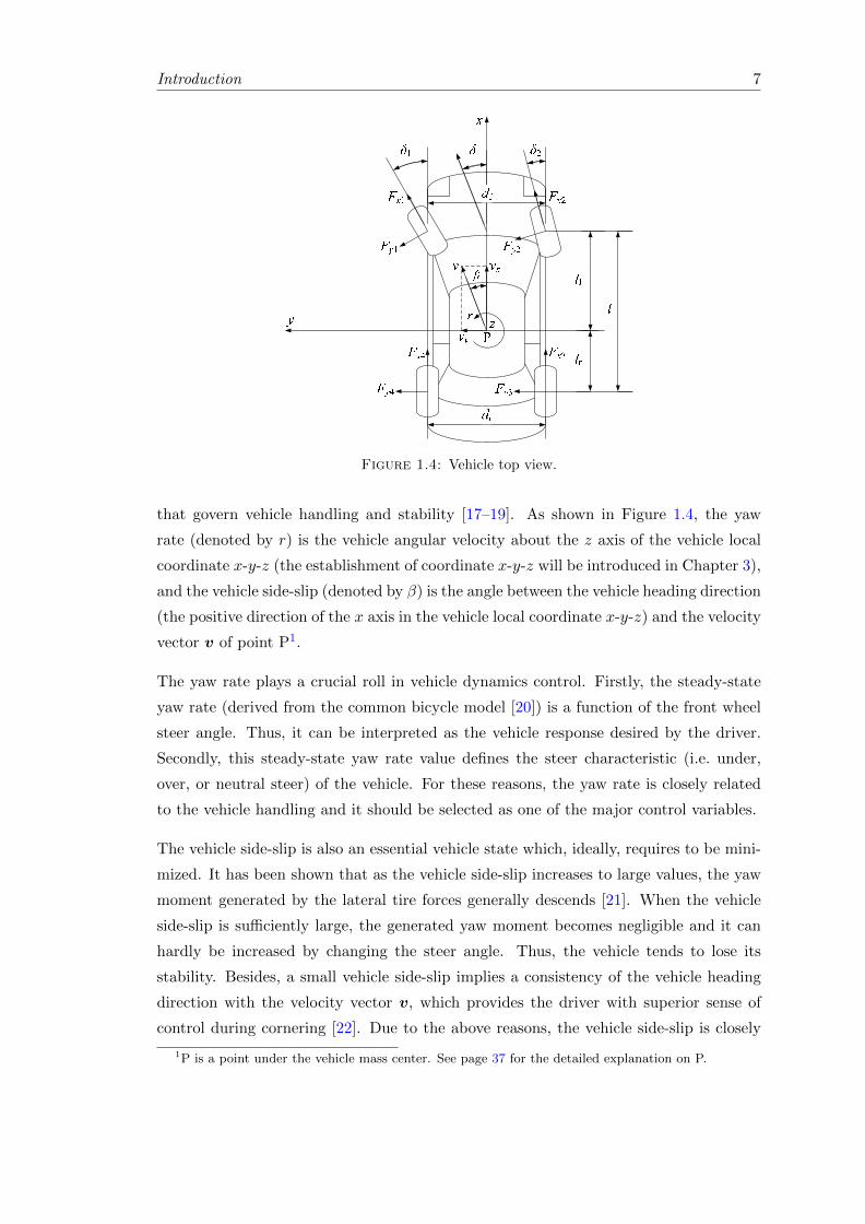
Figure 1.4: Vehicle top view.
that govern vehicle handling and stability [17–19]. As shown in Figure 1.4, the yaw
rate (denoted by r) is the vehicle angular velocity about the z axis of the vehicle local
coordinate x-y-z (the establishment of coordinate x-y-z will be introduced in Chapter 3),
and the vehicle side-slip (denoted by β) is the angle between the vehicle heading direction
(the positive direction of the x axis in the vehicle local coordinate x-y-z) and the velocity
vector v of point P1.
The yaw rate plays a crucial roll in vehicle dynamics control. Firstly, the steady-state
yaw rate (derived from the common bicycle model [20]) is a function of the front wheel
steer angle. Thus, it can be interpreted as the vehicle response desired by the driver.
Secondly, this steady-state yaw rate value defines the steer characteristic (i.e. under,
over, or neutral steer) of the vehicle. For these reasons, the yaw rate is closely related
to the vehicle handling and it should be selected as one of the major control variables.
The vehicle side-slip is also an essential vehicle state which, ideally, requires to be mini-
mized. It has been shown that as the vehicle side-slip increases to large values, the yaw
moment generated by the lateral tire forces generally descends [21]. When the vehicle
side-slip is sufficiently large, the generated yaw moment becomes negligible and it can
hardly be increased by changing the steer angle. Thus, the vehicle tends to lose its
stability. Besides, a small vehicle side-slip implies a consistency of the vehicle heading
direction with the velocity vector v, which provides the driver with superior sense of
control during cornering [22]. Due to the above reasons, the vehicle side-slip is closely
1P is a point under the vehicle mass center. See page 37 for the detailed explanation on P.
Introduction 8
connected to the vehicle stability and driver’s sense of control, and it should also be
chosen as the control variable.
Note that even though the yaw rate is more related to the vehicle handling and the
vehicle side-slip is mainly connected to the vehicle stability, these two vehicle states
are not independent, instead, they are intrinsically related by the vehicle dynamics (see
vehicle equations of motion in Chapter 3). Hence, they both affect the vehicle handling
and stability.
1.2.2 Research questions
Various DYC designs for controlling one or both of the above states have been introduced
in the literature. However, a basic question is often neglected by researchers and it has
not been well answered, which is: How does the additional yaw moment produced by
a DYC system change vehicle dynamics, i.e., what are the mathematical relationships
between the additional yaw moment and the vehicle states (yaw rate and vehicle side-
slip)?
The discovery of the above fundamental mathematical relationships should reveal the
essence of a DYC system, which leads to the second research question: How to design a
yaw rate-based or vehicle side-slip-based DYC system, based on the derived fundamental
mathematical relationships?
In order to improve DYC robustness as well as combine the benefits of controlling the
yaw rate and vehicle side-slip individually, many recent DYC works adopt both states
simultaneously as the control variables and such solutions have exhibited superior control
performance to the systems controlling one state only [17, 23–26]. However, in some
certain scenarios these solutions still present some imperfections and limitations. Thus,
the third research question is: How to design a DYC system to control both the yaw rate
and vehicle side-slip simultaneously, to improve the performance of the state-of-the-art
DYC systems?
The objectives of this thesis are to answer the above three research questions through
mathematical derivations and new DYC designs, and verify the proposed schemes by
means of extensive computer simulations. The following chapters will elaborate on the
design processes and verifications of the proposed DYC systems.
Introduction 9
1.3 CONTRIBUTIONS
The contributions of this study lie in three aspects. First of all, the fundamental math-
ematical correlations between the vehicle states (i.e. yaw rate and vehicle side-slip) and
the additional yaw moment generated by the DYC system are formulated and analyzed.
These relationships reveal how the DYC system influences the vehicle dynamics and pro-
vide implications for controller design. Secondly, based on the discovered relationships,
a yaw rate-based DYC system and a vehicle side-slip-based DYC system are proposed.
These systems are verified through extensive simulations to be effective in tracking the
desired yaw rate and desired vehicle side-slip, respectively. Lastly, a novel sliding mode
DYC scheme controlling both vehicle states is proposed to enhance the control perfor-
mance of the existing sliding mode DYC methods. Extensive simulations demonstrate
that the proposed method provides superior control performance to the conventional
solutions.
1.4 THESIS OUTLINE
This thesis consists of seven chapters. In Chapter 1, an introduction to the research
background, research scope and research questions is given. Then in Chapter 2, a
comprehensive literature review of various types of DYC systems, from the very basic
systems to the state-of-the-art DYC solutions, is presented.
In Chapter 3, a full vehicle model including the vehicle equivalent mechanical model,
vehicle equations of motion, wheel equation of motion and Magic Formula tire model is
established. The vehicle equations of motion governing the vehicle longitudinal, lateral,
roll and yaw motions are employed in Chapters 4–6 for DYC system design. The full
vehicle model is programed in MATLAB/Simulink environment to generate simulation
results.
In Chapter 4, based on the investigation of the vehicle equations of motion, a fundamen-
tal mathematical relation governing the yaw dynamics with a DYC system on-board is
derived. Based on this relationship, a yaw rate-based DYC system which aims to achieve
neutral steer performance is proposed. In Chapter 5, a similar mathematical equation
is derived for vehicle side-slip, based on which a vehicle side-slip-based DYC system
that tracks zero side-slip is devised. The yaw rate and vehicle side-slip-based DYC sys-
tems are verified through computer simulations to be effective in improving the vehicle
handling and stability, respectively.
Introduction 10
In Chapter 6, a new sliding mode-based DYC method is proposed for simultaneous
tracking of the desired yaw rate and vehicle side-slip. This DYC scheme directly employs
the complete nonlinear vehicle equations of motion established in Chapter 3 without
simplification to achieve a more effective control law. Also, the proposed DYC design
introduces a novel switching function that guarantees simultaneous convergences of both
the yaw rate and vehicle side-slip errors to zero. The effectiveness of the proposed DYC in
enhancing the vehicle handling and stability is verified through comparative simulations
in various challenging driving scenarios.
In Chapter 7, conclusions on the entire study are given and recommendations for future
work are presented.
Chapter 2
Literature Review
In this chapter, a comprehensive literature review of various types of DYC systems is
presented. Based on the control variable(s) used, the DYC systems are classified into
three main categories: the yaw rate-based DYC, the vehicle side-slip-based DYC and
the simultaneous control of the yaw rate and vehicle side-slip. In order to show how
DYC systems have evolved, two basic types of control systems for managing independent
electric motors, the equal torque methods and Ackerman methods, are introduced first.
For each type of control methods, the theoretical concepts and principles are summa-
rized, the features and characteristics are highlighted, and their control performances are
analyzed. This literature review lays the foundation for the analysis in the subsequent
chapters.
2.1 EQUAL TORQUE METHODS
The most straightforward way of controlling two independent motors is to send equal
torque commands to the two motors. The control methods using this approach are
referred to as the equal torque methods, and they emulate the behavior of an open
differential (the most used mechanical differential) which applies equal torques to both
wheels and allows speed differentiation at the same time. The equal torque methods
provide the electric vehicle with a cornering performance similar to an ICE vehicle
equipped with an open differential. Note that the equal torque methods cannot be
categorized as DYC systems, as no active yaw moment is generated to regulate the
vehicle motions. They are introduced here to show how simple control solutions evolved
to sophisticated DYC systems to enhance the control performance.
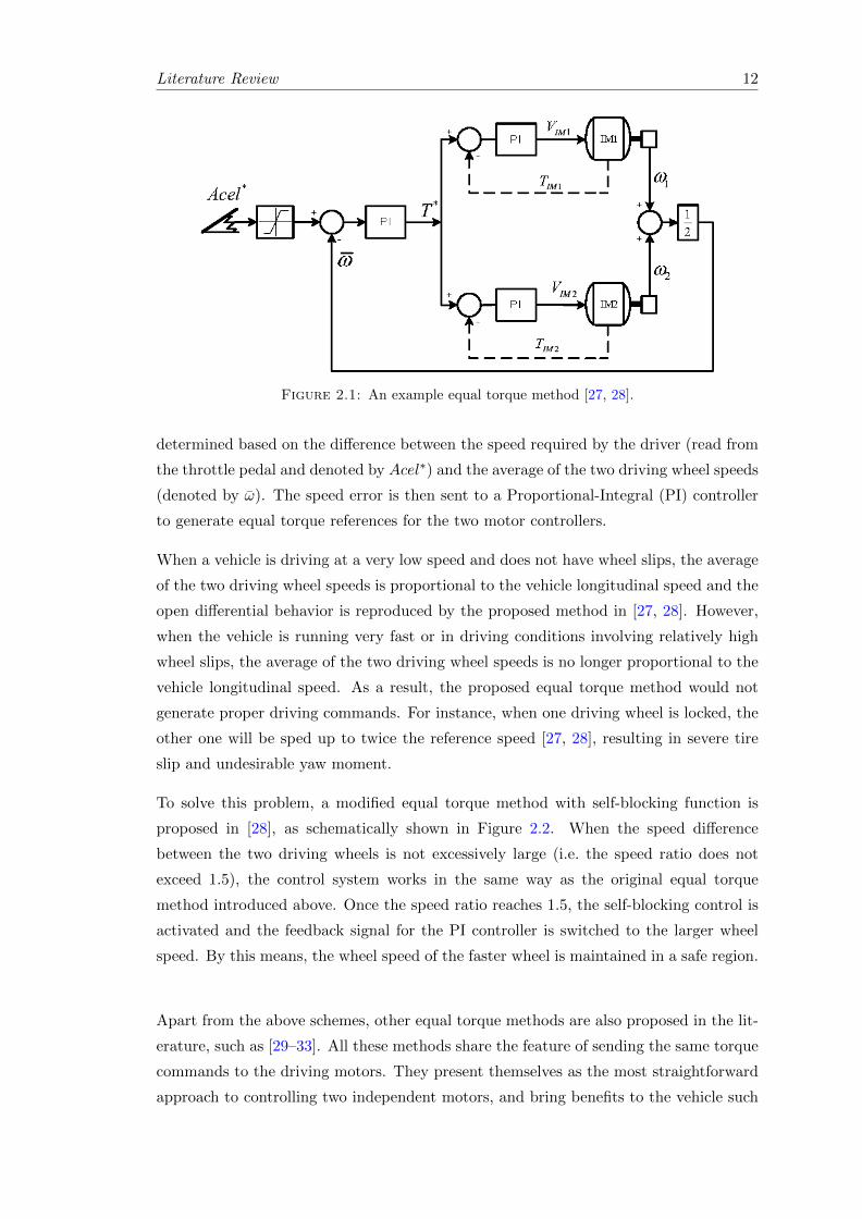
Magallan et al. proposed an equal torque method in their works [27, 28], as schematically
shown in Figure 2.1. In this solution, the torque commands sent to the motors are
11
Literature Review 12
124 G.A. Magallán, C.H. De Angelo and G.O. García
3.2 Electronic differential
As presented in a previous paper (Magallán et al., 2008), the present work implemented a simple differential traction control by emulating the mechanical differential behaviour. During this first vehicle control design stage, steering angle and vehicle speed were not measured; only speeds and currents of each motor were measured.
As can be seen in Figure 6, the accelerator pedal is the reference for the motor’s average speed. When the vehicle is moved in normal conditions (without slipping wheels), this reference is proportional to the vehicle speed:
1 2 .2 xr V
ω ω+=
where:
ω1 = wheel 1 angular speed
ω2 = wheel 2 angular speed
r = wheel radius
Vx = longitudinal vehicle speed.
Figure 6 Implemented equal torque differential control
A Proportional-Integral (PI) controller is used to control the average speed and its output is a torque reference for the traction motors’ controllers. This approach applies equal torques to each wheel for all the vehicle trajectories independent of wheel speeds. In this way, the mechanical differential behaviour is reproduced.
However, if a traction wheel is blocked or running free, the free wheel tends to accelerate up to twice the reference speed. This drawback can be easily avoided by limiting the maximum wheel speed in each wheel controller (see Section 3.3). Another trade off in using this simple equal torque control is produced during turning manoeuvres. Under good adhesion conditions, the inner curve wheel produces an opposite moment to the turn of the vehicle, hardening the steering and increasing vehicle losses. The same occurs in vehicles with conventional mechanical differentials.
Figure 2.1: An example equal torque method [27, 28].
determined based on the difference between the speed required by the driver (read from
the throttle pedal and denoted by Acel∗) and the average of the two driving wheel speeds
(denoted by ω). The speed error is then sent to a Proportional-Integral (PI) controller
to generate equal torque references for the two motor controllers.
When a vehicle is driving at a very low speed and does not have wheel slips, the average
of the two driving wheel speeds is proportional to the vehicle longitudinal speed and the
open differential behavior is reproduced by the proposed method in [27, 28]. However,
when the vehicle is running very fast or in driving conditions involving relatively high
wheel slips, the average of the two driving wheel speeds is no longer proportional to the
vehicle longitudinal speed. As a result, the proposed equal torque method would not
generate proper driving commands. For instance, when one driving wheel is locked, the
other one will be sped up to twice the reference speed [27, 28], resulting in severe tire
slip and undesirable yaw moment.
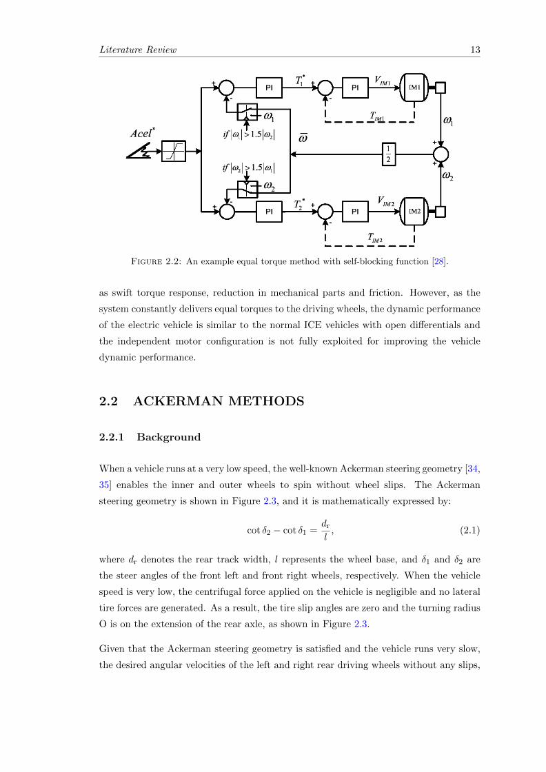
To solve this problem, a modified equal torque method with self-blocking function is
proposed in [28], as schematically shown in Figure 2.2. When the speed difference
between the two driving wheels is not excessively large (i.e. the speed ratio does not
exceed 1.5), the control system works in the same way as the original equal torque
method introduced above. Once the speed ratio reaches 1.5, the self-blocking control is
activated and the feedback signal for the PI controller is switched to the larger wheel
speed. By this means, the wheel speed of the faster wheel is maintained in a safe region.
Apart from the above schemes, other equal torque methods are also proposed in the lit-
erature, such as [29–33]. All these methods share the feature of sending the same torque
commands to the driving motors. They present themselves as the most straightforward
approach to controlling two independent motors, and bring benefits to the vehicle such
Literature Review 13
An NEV development with individual traction on rear wheels 125
More accurate and complex differential control schemes can be carried out by taking into account the geometry and vehicle dynamic models. In Cordeiro et al. (2006), Chen et al. (2007) and de Castro et al. (2007), vehicle speed, Vx, and steering angle, δ, were the input signals, and measured speeds of the inner and outer wheels were used. These approaches may present some drawbacks if any traction wheel is blocked, producing high and nonuniform torques and generating vehicle yaw movement. Some new strategies, based on the geometry and vehicle dynamic models, are being evaluated to improve the traction control implemented in the present paper.
3.3 Electronic self-blocking differential
As stated above, with the implemented traction differential scheme, if any drive wheel lost traction (e.g., for different road conditions in each wheel), it would tend to accelerate until double speed reference. To avoid this behaviour, a basic self-blocking differential control is performed as shown in Figure 7.
Figure 7 Self-blocking differential control
While the magnitude of the speed differential ratio on the traction wheels is maintained below 1.5, the self-blocking behaviour is identical to the equal-torque differential control (Figure 6). Once this value (difference of 1.5 times) is reached (e.g., during a wheel skidding), the self-blocking control switches to the two individual speed controls on each traction wheel.
In this situation, each wheel speed control receives the same reference and the feedback signals are switched to the individual motor speeds measurement. In this way the wheels traction speeds are maintained under safe operation.
Once the self-blocking control is activated, the return to the equal-torque control is performed when the differential speed decreases below 1.5 and an additional significant torque current exists (at least 5% of the rated current). This condition would indicate that the vehicle is in normal traction conditions. This hysteresis control prevents the oscillating behaviour in the transition.
Figure 2.2: An example equal torque method with self-blocking function [28].
as swift torque response, reduction in mechanical parts and friction. However, as the
system constantly delivers equal torques to the driving wheels, the dynamic performance
of the electric vehicle is similar to the normal ICE vehicles with open differentials and
the independent motor configuration is not fully exploited for improving the vehicle
dynamic performance.
2.2 ACKERMAN METHODS
2.2.1 Background
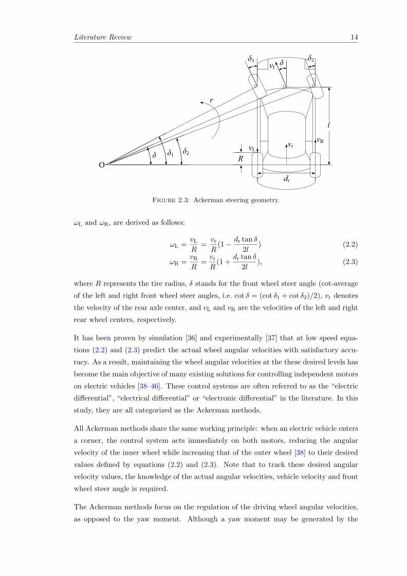
When a vehicle runs at a very low speed, the well-known Ackerman steering geometry [34,
35] enables the inner and outer wheels to spin without wheel slips. The Ackerman
steering geometry is shown in Figure 2.3, and it is mathematically expressed by:
cot δ2 − cot δ1 =drl, (2.1)
where dr denotes the rear track width, l represents the wheel base, and δ1 and δ2 are
the steer angles of the front left and front right wheels, respectively. When the vehicle
speed is very low, the centrifugal force applied on the vehicle is negligible and no lateral
tire forces are generated. As a result, the tire slip angles are zero and the turning radius
O is on the extension of the rear axle, as shown in Figure 2.3.
Given that the Ackerman steering geometry is satisfied and the vehicle runs very slow,
the desired angular velocities of the left and right rear driving wheels without any slips,
Literature Review 14
δ
l
R
vr
r
δ
dr
vL
vR
vfδ2δ1
δ1 δ2
Figure 2.3: Ackerman steering geometry.
ωL and ωR, are derived as follows:
ωL =vLR
=vrR
(1− dr tan δ
2l) (2.2)
ωR =vRR
=vrR
(1 +dr tan δ
2l), (2.3)
where R represents the tire radius, δ stands for the front wheel steer angle (cot-average
of the left and right front wheel steer angles, i.e. cot δ = (cot δ1 + cot δ2)/2), vr denotes
the velocity of the rear axle center, and vL and vR are the velocities of the left and right
rear wheel centers, respectively.
It has been proven by simulation [36] and experimentally [37] that at low speed equa-
tions (2.2) and (2.3) predict the actual wheel angular velocities with satisfactory accu-
racy. As a result, maintaining the wheel angular velocities at the these desired levels has
become the main objective of many existing solutions for controlling independent motors
on electric vehicles [38–46]. These control systems are often referred to as the “electric
differential”, “electrical differential” or “electronic differential” in the literature. In this
study, they are all categorized as the Ackerman methods.
All Ackerman methods share the same working principle: when an electric vehicle enters
a corner, the control system acts immediately on both motors, reducing the angular
velocity of the inner wheel while increasing that of the outer wheel [38] to their desired
values defined by equations (2.2) and (2.3). Note that to track these desired angular
velocity values, the knowledge of the actual angular velocities, vehicle velocity and front
wheel steer angle is required.
The Ackerman methods focus on the regulation of the driving wheel angular velocities,
as opposed to the yaw moment. Although a yaw moment may be generated by the
Literature Review 15
����������������� �����������������������������������������������������������������
���
������������ �!����������� ���������������
����"���#$���%���������&���'������������#$��������������� (�)*+,-����#$���&���.���&����/�01+�* 2+3(,,,,����4/�01+�* 2+3 �-2(��
�
� �������������5��������6��7��������"'���������8��$�����7��9�7�����&������,)(*,,��8��$����&���.���&����/�01+�* �-)�323�����4/�01+�* �-)�3�23��
����/����������� �� ������������� �� ��������������� �� ����
��
��������:� ���� ��� ������� ����� ���� ���� ����������� ������������������������������������������������������ ����������������������������������������������������������������������������������������������������������������������������������������������������������������������������� ���������������������������������������������������������������� ���������� ��� ���� ������� ��� �� ������� ��������� ����� !���������������������������� ����� �������� �������� ��������� �� ���������� ��� �� ���������������������� !�"#$%&'����
(�������)� ���������� ������ ������ ������� 7������� �������������������
%� %;"9<�6 "%<;�"��� ���������� ��� ��7�����.� ������� 7������� �����
.���������������������$����� �����������������.������� ���� ��������� ����� �� .�$�� ����*�������� �����.��� "����������.���� ��7������ ��� ��7��� ����� ��7�� ������ ����������������������=�����$������.������������7������������������������������������������������>�����
6���.� ������� ������ ������� ��� �7���� �� ���������������������.��������7����������������$���������������$��>��������������������7���?�������������������������.�����.�$��������������������������������������������
"������������������ ���$�������� ����7���.���=�������������� � � ������ $���.� ���� ��������� ��� ��������� �������������������������������
"���������������������������� �����������$�������.����������������������������.���������������$������������*���� ����������� �=������� ������ ����� ������@��.� ���������� ��� ��� ����� ������� ��>��.� ����� �������� �����$���������������������������$�������������������
"��� �4��������� ������ ��������� ���� �$������� ������ ������� ��� ���� �$������ ���� ��� �� ����� ��� ���� 7����������������������������
�
%%� �8� "9% ��%!!�9�;"%�8�!<9��8� "9% ���A% 8��?%"A�"?<�%;��&�;��;"�?A��8��9%�����
� �� ������ ���� �������������"���7���������� ���� ������������ ����������7��������
�����������������B��.����C��������������7����������������� ��������� ��.���� $������ � � ����� ���� $�� �� �������� *� ����7������
�� .����.� ��.���� �������� ��������� ������������� ����7��� ������ �������� $�� �� ���.�� ������������ ������������� ���� ����@��� ����� ���� ���� ��������� ����� ����������.� ��.��� �������.� 7���.�� ���� ������ ���� $���������� ��� ������ ���� ��������� ������ ����������� �����������
δ
M2
DC/DCConverter
1
Batteries
M1
Accelerator
DC/DCConverter
2
"
'
*
%
�.�D��
�.�D��
�����
�����
�
!�.������ ����.�����������������������������7�������
IEEE MELECON 2006, May 16-19, Benalmádena (Málaga), Spain
1-4244-0088-0/06/$20.00 ©2006 IEEE 1174
Figure 2.4: Electric vehicle configuration proposed by Cordeiro et al. [39].
control methods in the course of angular velocity regulation, the moment is not directly
controlled. Thus, the Ackerman methods are not categorized as DYC systems, either.
They are introduced here to show how control solutions evolved from simple methods
to sophisticated DYC systems.
2.2.2 Control methods based on Ackerman steering geometry
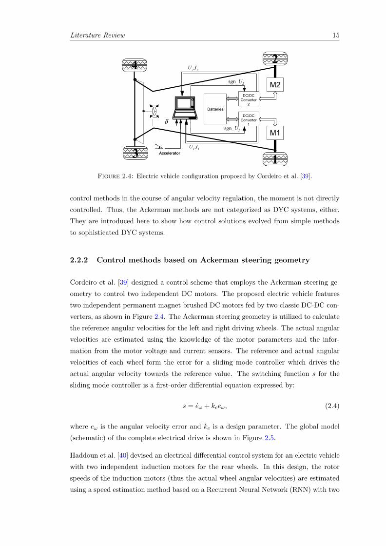
Cordeiro et al. [39] designed a control scheme that employs the Ackerman steering ge-
ometry to control two independent DC motors. The proposed electric vehicle features
two independent permanent magnet brushed DC motors fed by two classic DC-DC con-
verters, as shown in Figure 2.4. The Ackerman steering geometry is utilized to calculate
the reference angular velocities for the left and right driving wheels. The actual angular
velocities are estimated using the knowledge of the motor parameters and the infor-
mation from the motor voltage and current sensors. The reference and actual angular
velocities of each wheel form the error for a sliding mode controller which drives the
actual angular velocity towards the reference value. The switching function s for the
sliding mode controller is a first-order differential equation expressed by:
s = eω + keeω, (2.4)
where eω is the angular velocity error and ke is a design parameter. The global model
(schematic) of the complete electrical drive is shown in Figure 2.5.
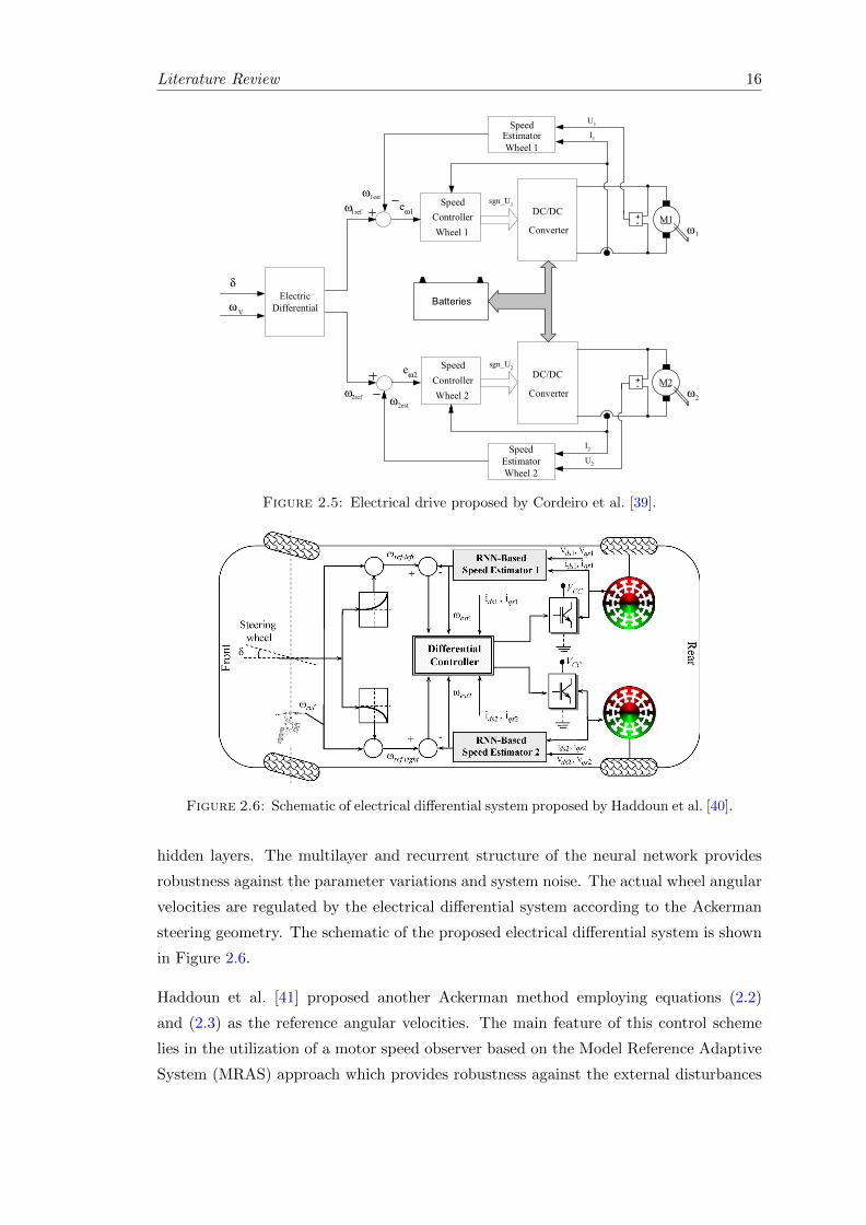
Haddoun et al. [40] devised an electrical differential control system for an electric vehicle
with two independent induction motors for the rear wheels. In this design, the rotor
speeds of the induction motors (thus the actual wheel angular velocities) are estimated
using a speed estimation method based on a Recurrent Neural Network (RNN) with two
Literature Review 16
� �� ����� � �� ���� �� ����� �!�.��� �������������7������������������.�������.��
������������������������$������������������.���.������������������������$������������������������������4����
"�������������$�������������.����������ω������ω��������� ����� ��7��� ��� �4����� $�� �=������� B�C�� "��� ������.���.����.�������������������7�����������E F��
8
9
�
������.ωωωω "
ωωωω '
δ
δ
��������"��
M
M
�
!�.��� �� �����������.�������.��
?����δ = 0��������7�����$�������.�����.����������
����� ωδωωω =−=Δ � � B�C
"�����.������������������ω�� ������ω�� ����������������7����������������������������������������������������� ����������������!�.���1� ��� �� ���.��� ����� �������������7�����������������������������ω���������������������������������������������������
( ) � ωδω �=Δ
�ωωω Δ+=
ωωω Δ−=
δ
ω�� �
ω
ω�� �
�
!�.���1�� ���������������������.����
! "�����#�� ����� � ����������� !�.���)�������������$��>����.����������.�$�������
��� ���� �������� ��7�� �������� ��� .�������� ���� ������������������������������7�����
δ
6�
ω���
ω�
ω ��
ω �
��
�������������?����
� G�
��7���
����� �����?�����
����������������
����� �����?����
� G�
��7����
�ω1
�ω2
ω
%�
�.�D6�
�.�D6
+-
+-
% 6
Batteries
�������������?�����
ω����
ω ���
�
!�.���)�� ����������7���
%%%� �&������"%��"%<;��� 7���.�� ���� �� ������ ������ ��� ����������� ��7����
������������� ��.���� ��� ���� ���� ������ ���������������� ���$������������������.��=�������B CE�F/�
φω
$
����� �� %
����� �−−= � B C�
�"���� ������� �������� ���� �������� ���������
>�����.��� "��� ��������� �������.� ���� ���7���$��������� ���� 7���� ��� ���� ���������� ������ ω ���� $���.� �����$������7�������������� ��ωωω −=H ��4�������$��B1C/�
( )��
� �� � � �
$ $
� �� �
% %φφ
ω ε ω ε εφ φε
� �� � � �= + +� �� �
− � � � �� �� � B1C�
�
�����ε���ε���εφ����������������7������������7����������������� ������� ����������� ������� ������.� ����������� �������4�����������
!�.��� +� �������� ���� ���������� ���� ���� �4��������������� ��� ���� ������ ����������� ��� �� ���.�� ����� ����.� �������������������������������������������.���.� δ = 0.
Whe
el S
peed
[rpm
]
t [s]
-500
0
-500
0
500
0
500
0 1 2 3 4 5 6 7 8 9 10
ωωωωref
ωωωωm
ωωωωest
��C�
�$C�
!�.���+�� ���������$��������������������������������������������I��C������������$C��4����������
�� ���������� $������� ���� ����������� ω ���� ���� ������������������B�����.������C��ω#������������������
1175
Figure 2.5: Electrical drive proposed by Cordeiro et al. [39].2290 IEEE TRANSACTIONS ON INDUSTRIAL ELECTRONICS, VOL. 55, NO. 6, JUNE 2008
Fig. 4. EV propulsion and control systems schematic diagram.
Fig. 5. Driving trajectory model.
Fig. 6. Block diagram of the electric differential system.
summarized in the Appendix (Fig. 7). Electrical vehicle me-chanical and aerodynamic characteristics are also given in theAppendix. Objectives of the simulations carried out were to
assess the efficiency and dynamic performance of the proposedneural network control strategy.
The test cycle is the urban ECE-15 cycle (Fig. 8) [30].A driving cycle is a series of data points representing the vehiclespeed versus time. It is characterized by low vehicle speed(maximum 50 km/h) and is useful for testing electrical vehicleperformance in urban areas.
The electric differential performances are first illustrated byFig. 9, which shows each wheel’s drive speed during steeringfor 0 < t < 1180 s. It is obvious that the electric differentialoperates satisfactorily according to the complicated series ofaccelerations, decelerations, and frequent stops imposed by theurban ECE-15 cycle.
Figs. 10 and 11 illustrate the EV dynamics, respectively, theflux (λdr) and the developed torque in each induction motor onthe left and right wheel drives, with changes in the acceleration
Figure 2.6: Schematic of electrical differential system proposed by Haddoun et al. [40].
hidden layers. The multilayer and recurrent structure of the neural network provides
robustness against the parameter variations and system noise. The actual wheel angular
velocities are regulated by the electrical differential system according to the Ackerman
steering geometry. The schematic of the proposed electrical differential system is shown
in Figure 2.6.
Haddoun et al. [41] proposed another Ackerman method employing equations (2.2)
and (2.3) as the reference angular velocities. The main feature of this control scheme
lies in the utilization of a motor speed observer based on the Model Reference Adaptive
System (MRAS) approach which provides robustness against the external disturbances
Literature Review 17
and system uncertainties. The actual angular velocities are estimated by the MRAS-
based observer, and are fed back to an electric differential system to regulate the wheel
angular velocities.
In the works of Zhao et al. [42, 43], an electronic differential system is designed for an
electric vehicle with two Permanent Magnet Brushless Direct Current Motors (PMBD-
CMs). A fuzzy logic control algorithm is employed in this design to achieve the desired
wheel angular velocities derived from the Ackerman steering geometry.
Perez-Pinal et al. [44] proposed an electric differential design for a rear-wheel-drive
electric vehicle. This solution employs a motor synchronization control approach, aiming
to prevent deviation from the desired vehicle path. The synchronization strategy is
realized through a fictitious general master controller which provides each wheel with a
speed reference based on the Ackerman steering geometry.
In the work of Nasri et al. [45], a fuzzy logic control scheme is applied to control the
two independent induction motors to obtain better efficiency and enhanced robustness
against the parameter variation. In this design, the Ackerman steering geometry is
employed to compute the speed references for the two driving motors.
The Ackerman steering geometry can also be employed in the control designs for 4-
Wheel-Drive (4WD) electric vehicles. Zhou et al. [46] developed an electronic differen-
tial system for controlling a prototype electric vehicle with four brushless DC in-wheel
motors. When the vehicle moves in a straight line, this control system ensures that all
wheels rotate at the same speed as the slowest one, if they are not consistent. When
the vehicle makes a turn, the controller adjusts the wheel angular velocities to the de-
sired levels derived from the Ackerman steering geometry. Meanwhile, the vehicle speed
during cornering is held constant by the controller.
2.2.3 Remarks
It is important to note that the Ackerman steering geometry is a purely kinematic con-
dition that is accurate only when the vehicle speed is very low. This is because the
centrifugal force and tire slip angles are neglected in the Ackerman steering geometry.
As a result, neither the tire cornering characteristics nor the vehicle dynamics is taken
into account. On the other hand, the desired wheel angular velocities derived from the
Ackerman steering geometry assume no wheel slips. In reality, wheel slips are ubiqui-
tous in various driving conditions, and absolute zero wheel slip is impractical. For these
reasons, control designs based on the Ackerman steering geometry are only suitable for
Literature Review 18
certain low-speed vehicle applications in which the tire slips are negligible during corner-
ing. In the following chapters, simulation results obtained from high speed maneuvers
will expose the inherent shortcomings of the Ackerman steering geometry-based control
solutions.
2.3 YAW RATE-BASED DYC
2.3.1 Background
As discussed in the preceding sections, both the equal torque methods and Ackerman
methods present obvious downsides and do not provide optimum control performances.
This has led researchers to seek new control solutions towards making full advantage
of independent driving motors and achieving better control performance. In this effort,
various DYC designs have been proposed in the literature. The major advantage of DYC
systems over the previous two types of methods is that they take the vehicle dynamics
into account, and directly adjust the yaw moment generated by the individual motor
torques to regulate the target vehicle state(s) and in turn remould the vehicle dynamics.
It has been pointed out in Chapter 1 that the yaw rate r plays a crucial role in vehicle
dynamics and should be selected as the control variable in DYC systems. In the litera-
ture, numerous DYC designs have been proposed to drive the actual yaw rate towards a
desired (reference) yaw rate value, aiming to enhance the vehicle handling and stability.
The vast majority of existing DYC solutions employ the steady-state yaw rate response
(or its variation/modification) derived from the two Degree-of-Freedom (DoF) planar
vehicle model (bicycle model) [20] as the desired (reference) yaw rate. This value can
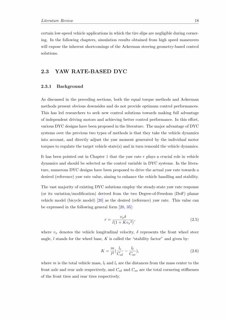
be expressed in the following general form [20, 35]:
r =vxδ
l(1 +Kvx2), (2.5)
where vx denotes the vehicle longitudinal velocity, δ represents the front wheel steer
angle, l stands for the wheel base, K is called the “stability factor” and given by:
K =m
l2(lrCαf− lfCαr
), (2.6)
where m is the total vehicle mass, lf and lr are the distances from the mass center to the
front axle and rear axle respectively, and Cαf and Cαr are the total cornering stiffnesses
of the front tires and rear tires respectively.
Literature Review 19
On the one hand, the above steady-state yaw rate response is a reflection of the driver’s
control inputs. It is seen that the yaw rate r is a function of the front wheel steer angle δ
and the vehicle longitudinal velocity vx. Because δ is commanded by the driver through
steering wheel and vx is controlled by the driver via throttle or brake pedal, therefore
the yaw rate response given by equation (2.5) can be interpreted as the steady-state
vehicle response desired by the driver.
On the other hand, by means of vehicle turning radius, this yaw rate response defines
the vehicle’s steer characteristic which affects the vehicle handling and stability. The
vehicle steady-state turning radius can be derived from the yaw rate response equation.
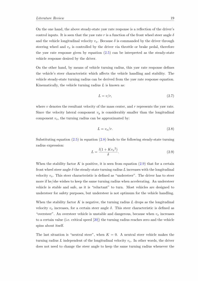
Kinematically, the vehicle turning radius L is known as:
L = v/r, (2.7)
where v denotes the resultant velocity of the mass center, and r represents the yaw rate.
Since the velocity lateral component vy is considerably smaller than the longitudinal
component vx, the turning radius can be approximated by:
L = vx/r. (2.8)
Substituting equation (2.5) in equation (2.8) leads to the following steady-state turning
radius expression:
L =l(1 +Kvx
2)
δ. (2.9)
When the stability factor K is positive, it is seen from equation (2.9) that for a certain
front wheel steer angle δ the steady-state turning radius L increases with the longitudinal
velocity vx. This steer characteristic is defined as “understeer”. The driver has to steer
more if he/she wishes to keep the same turning radius when accelerating. An understeer
vehicle is stable and safe, as it is “reluctant” to turn. Most vehicles are designed to
understeer for safety purposes, but understeer is not optimum for the vehicle handling.
When the stability factor K is negative, the turning radius L drops as the longitudinal
velocity vx increases, for a certain steer angle δ. This steer characteristic is defined as
“oversteer”. An oversteer vehicle is unstable and dangerous, because when vx increases
to a certain value (i.e. critical speed [20]) the turning radius reaches zero and the vehicle
spins about itself.
The last situation is “neutral steer”, when K = 0. A neutral steer vehicle makes the
turning radius L independent of the longitudinal velocity vx. In other words, the driver
does not need to change the steer angle to keep the same turning radius whenever the
Literature Review 20
vehicle accelerates or decelerates in a corner. Neutral steer is the ideal steer character-
istic, as it not only keeps the vehicle stable but also provides good handling. However,
it is impractical to constantly maintain neutral steer (i.e. K = 0) without any electronic
systems, because the stability factor K is a function of the cornering stiffnesses Cαf and
Cαr which constantly change with the driving condition.
To sum up, the steady-state yaw rate response, equation (2.5), not only represents
the vehicle response commanded by the driver, but also influences the vehicle handling
and stability through the stability factor K. In the following section, the typical yaw
rate-based DYC solutions that employ equation (2.5) (or its variation/modification)
as the desired (reference) response are reviewed. Note that apart from the yaw rate-
based DYC systems with independent motor configuration, other typical yaw rate-based
DYC solutions such as the differential braking systems and active differentials are also
reviewed, since they share similar design principles and provide insights into new DYC
design.
2.3.2 Typical yaw rate-based DYC methods
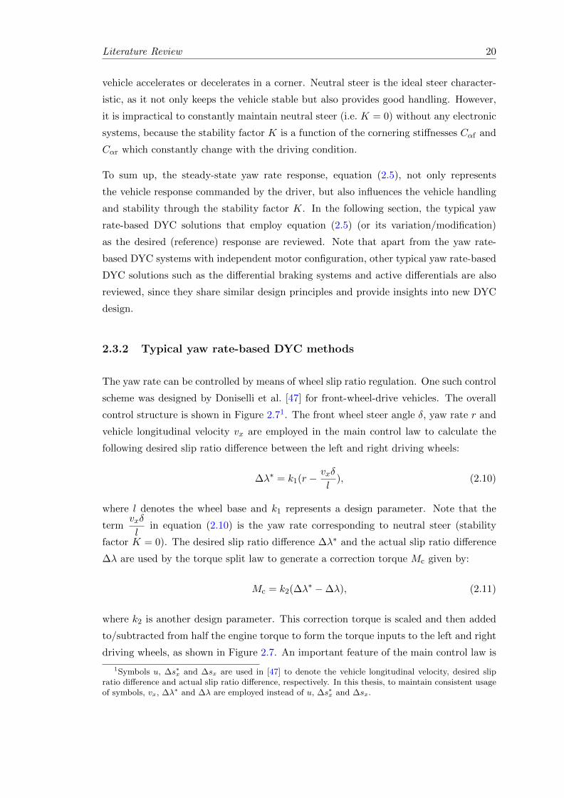
The yaw rate can be controlled by means of wheel slip ratio regulation. One such control
scheme was designed by Doniselli et al. [47] for front-wheel-drive vehicles. The overall
control structure is shown in Figure 2.71. The front wheel steer angle δ, yaw rate r and
vehicle longitudinal velocity vx are employed in the main control law to calculate the
following desired slip ratio difference between the left and right driving wheels:
∆λ∗ = k1(r −vxδ
l), (2.10)
where l denotes the wheel base and k1 represents a design parameter. Note that the
termvxδ
lin equation (2.10) is the yaw rate corresponding to neutral steer (stability
factor K = 0). The desired slip ratio difference ∆λ∗ and the actual slip ratio difference
∆λ are used by the torque split law to generate a correction torque Mc given by:
Mc = k2(∆λ∗ −∆λ), (2.11)
where k2 is another design parameter. This correction torque is scaled and then added
to/subtracted from half the engine torque to form the torque inputs to the left and right
driving wheels, as shown in Figure 2.7. An important feature of the main control law is
1Symbols u, ∆s∗x and ∆sx are used in [47] to denote the vehicle longitudinal velocity, desired slipratio difference and actual slip ratio difference, respectively. In this thesis, to maintain consistent usageof symbols, vx, ∆λ∗ and ∆λ are employed instead of u, ∆s∗x and ∆sx.
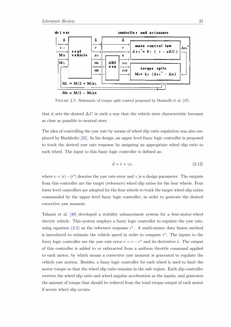
Literature Review 21to be applied at the driving wheels.
dr i ver controlle r and actuators
ML = M I 2 + M c k ~
Fig.3. Logical scheme of torque split control (symbols are explained in 5 3.2)
The signals ax, UR and UL are processed, exactly as implemented in some ABS [20], in order to get the longitudinal vehicle velocity u and 'the longitudinal slips at the wheels s x ~ and S ~ R . The. main control law processes r, u and 6 and sets the required difference of longitudinal slips at the driving wheels
(I: wheelbase, k ~ : parameter. sxl SXR : actual slips at time t)). This law has been derived by the authors starting from two basic considerations (commented extensively in 5 3.2.1 and in 5 3.2.2) which refer to the two previously mentioned enhancements of vehicle dynamic behaviours, i.e. maximum reachable centripetal acceleration aymu and minjmun response time to a steering-wheel step-input Tr. Due to a convenient occurrence, both these two peculiar dynamic behaviours of automobiles can be enhanced by the same control law (3.1). This law is linear but it is well suited and very effective to control non-linear systeqs too (see e.g. [I, 51).
As the required A s x has been set, a problem arises about how to get it at the wheels. Actuators are needed, and their characteristics are in general non-linear. So, the derivation of a control scheme, expressely studied for the operation of the actuators, is necessary:
M is the torque from the engine; h and lm are functions of sxt and S ~ R , res ctively (they are introduced to improve the response to p-split only (see 5 E . 3 )
Dow
nloa
ded
by [
RM
IT U
nive
rsity
] at
23:
13 1
5 Ju
ly 2
014
Figure 2.7: Schematic of torque split control proposed by Doniselli et al. [47].
that it sets the desired ∆λ∗ in such a way that the vehicle steer characteristic becomes
as close as possible to neutral steer.
The idea of controlling the yaw rate by means of wheel slip ratio regulation was also em-
ployed by Buckholtz [25]. In his design, an upper level fuzzy logic controller is proposed
to track the desired yaw rate response by assigning an appropriate wheel slip ratio to
each wheel. The input to this fuzzy logic controller is defined as:
d = e+ γe, (2.12)
where e = |r|− |r∗| denotes the yaw rate error and γ is a design parameter. The outputs
from this controller are the target (reference) wheel slip ratios for the four wheels. Four
lower level controllers are adopted for the four wheels to track the target wheel slip ratios
commanded by the upper level fuzzy logic controller, in order to generate the desired
corrective yaw moment.
Tahami et al. [48] developed a stability enhancement system for a four-motor-wheel
electric vehicle. This system employs a fuzzy logic controller to regulate the yaw rate,
using equation (2.5) as the reference response r∗. A multi-sensor data fusion method
is introduced to estimate the vehicle speed in order to compute r∗. The inputs to the
fuzzy logic controller are the yaw rate error e = r − r∗ and its derivative e. The output
of this controller is added to or subtracted from a uniform throttle command applied
to each motor, by which means a corrective yaw moment is generated to regulate the
vehicle yaw motion. Besides, a fuzzy logic controller for each wheel is used to limit the
motor torque so that the wheel slip ratio remains in the safe region. Each slip controller
receives the wheel slip ratio and wheel angular acceleration as the inputs, and generates
the amount of torque that should be reduced from the total torque output of each motor
if severe wheel slip occurs.
Literature Review 22
In the work of Motoyama et al. [49], a control method is proposed for traction force dis-
tribution between the left and right driving wheels. An ordinary Proportional-Derivative
(PD) controller is employed to control the vehicle yaw rate, aiming to achieve neutral
steer characteristic. This PD control law is written as:
α = α′ +K1(r − r∗) +K2(r − r∗), (2.13)
where r and r∗ are the actual yaw rate and desired yaw rate (expressed by equation (2.5)
with K = 0), respectively, K1 and K2 are the control parameters of the PD controller,
α denotes the traction force distribution ratio between the left and right wheels, and α′
represents the distribution ratio at the last sampling time.
Zhou and Liu [50] proposed a vehicle yaw stability control system using equation (2.5)
as the desired (reference) yaw rate response. This cascade yaw stability control system
consists of two interconnected parts. In the first part, a Sliding Mode Observer (SMO)
is employed to estimate the longitudinal and lateral tire forces which are used to update
the time-varying parameters in the vehicle and wheel models. In the second part, the
control input is computed in a backstepping control framework and through sliding mode
control in each step.
Nam et al. [51] developed an adaptive sliding mode control design for robust yaw stabi-
lization of an electric vehicle with two rear in-wheel motors. A sliding mode controller
is adopted in this design to make the vehicle track the desired yaw rate r∗, which is
defined as:
r∗ =r′
1 + τp, (2.14)
where r′ is the same reference yaw rate as equation (2.5), τ denotes the time constant
and p represents the Laplace transform variable. This low-pass filter,1
1 + τp, is used
to filter out the noise in the reference yaw rate signal. Besides, a parameter adaptation
law is employed to estimate the changing vehicle parameters and is incorporated into
the sliding mode control framework, which compensates the parameter uncertainties
and disturbances that vary with the driving condition. In the work of Yamamoto [52], a
desired yaw rate in the same form as equation (2.14) is employed. To track this reference
value, a control law is designed as follows:
∆Fx = k(r∗ − r), (2.15)
where ∆Fx denotes the longitudinal tire force difference between the left and right
driving wheels, k represents the control parameter, and r∗ and r are the desired and
actual yaw rates, respectively.
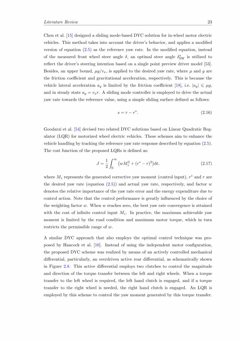
Literature Review 23
Chen et al. [15] designed a sliding mode-based DYC solution for in-wheel motor electric
vehicles. This method takes into account the driver’s behavior, and applies a modified
version of equation (2.5) as the reference yaw rate. In the modified equation, instead
of the measured front wheel steer angle δ, an optimal steer angle δ∗SW is utilized to
reflect the driver’s steering intention based on a single point preview driver model [53].
Besides, an upper bound, µg/vx, is applied to the desired yaw rate, where µ and g are
the friction coefficient and gravitational acceleration, respectively. This is because the
vehicle lateral acceleration ay is limited by the friction coefficient [18], i.e. |ay| 6 µg,
and in steady state ay = vxr. A sliding mode controller is employed to drive the actual
yaw rate towards the reference value, using a simple sliding surface defined as follows:
s = r − r∗. (2.16)
Goodarzi et al. [54] devised two related DYC solutions based on Linear Quadratic Reg-
ulator (LQR) for motorized wheel electric vehicles. These schemes aim to enhance the
vehicle handling by tracking the reference yaw rate response described by equation (2.5).
The cost function of the proposed LQRs is defined as:
J =1
2
∫ ∞
0
(wM2
z + (r∗ − r)2)dt, (2.17)
where Mz represents the generated corrective yaw moment (control input), r∗ and r are
the desired yaw rate (equation (2.5)) and actual yaw rate, respectively, and factor w
denotes the relative importance of the yaw rate error and the energy expenditure due to
control action. Note that the control performance is greatly influenced by the choice of
the weighting factor w. When w reaches zero, the best yaw rate convergence is attained
with the cost of infinite control input Mz. In practice, the maximum achievable yaw
moment is limited by the road condition and maximum motor torque, which in turn
restricts the permissible range of w.
A similar DYC approach that also employs the optimal control technique was pro-
posed by Hancock et al. [10]. Instead of using the independent motor configuration,
the proposed DYC scheme was realized by means of an actively controlled mechanical
differential, particularly, an overdriven active rear differential, as schematically shown
in Figure 2.8. This active differential employs two clutches to control the magnitude
and direction of the torque transfer between the left and right wheels. When a torque
transfer to the left wheel is required, the left hand clutch is engaged, and if a torque
transfer to the right wheel is needed, the right hand clutch is engaged. An LQR is
employed by this scheme to control the yaw moment generated by this torque transfer.
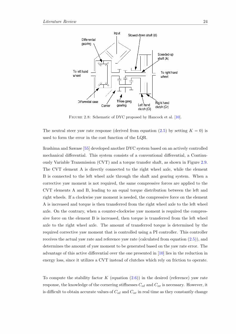
Literature Review 24
310 M J Hancock, R A Williams, T J Gordon, and M C Best
control system, but the relative merits of the twosystems and the benefits gleaned from integrationare not discussed in great detail [8].
The present paper investigates the potential ofan active overdriven differential to control the yawmoment of a vehicle and offers a comparison with abrake-based system.
2 VEHICLE MODEL
2.1 Chassis model
To facilitate the investigation, a vehicle handlingFig. 1 Overdriven differential schematicmodel was created. The main features of this model
are highlighted below (a more detailed descriptioncan be found in Appendix 2):
engaged. Provided a sufficient speed difference is(a) four degrees of freedom (4DOF): longitudinal,present, the target torque transfer will be achievedlateral, yaw, and roll;(see section 3.4.1).(b) rear-wheel drive;
The relationship between the input torque, clutch(c) non-linear tyres (utilizes version 94 of the magictorques, and driveshaft torques can be described asformula tyre model);follows [8](d) longitudinal and lateral weight transfer;
(e) compliance in the steering system.Tl=
Ti2−
z1z5
2z4z2DTcr+
z1z6
2z3z4DTcl
(1)
Note that aerodynamic drag and driveline dynamicsare not included in the model (driving/braking
Tr=Ti2+A1− z
1z5
2z4z2BDTcr−A1− z
1z6
2z3z4BDTcl (2)
torques are thus applied directly to the wheels). TheSAE sign convention was employed and is used
These relationships were used to represent an over-throughout this paper.driven differential in the vehicle model, and theirTo facilitate the analysis of the behaviour of thederivation is detailed in Appendix 3.vehicle model, a simple driver model was also
employed. The objective of this model was to controlthe steering of the vehicle to follow any predefined
3 CONTROLLER DESIGNtrajectory as precisely as possible. The demandedtrajectory is defined as a series of points, and the
In order to analyse the potential impact thatmodel operates by selecting the most appropriatecontrolled differentials can have on yaw–sideslip‘target point’ ahead of it using a variable previewdynamics, it is firstly necessary to develop ansystem. A proportional, integral, and derivative (PID)appropriate yaw moment control algorithm.controller then uses the error between the yaw angle
required to reach this point and the actual yaw rate3.1 Design structureto give the required steering angle.
It was considered essential that the yaw momentcontroller be designed using a formal methodology,
2.2 Differential modelparticularly in the light of the planned comparisonwith ABC. Such an approach was intended to ensureA schematic of the type of overdriven differential
considered in this paper is shown in Fig. 1. The that a meaningful evaluation of the abilities of theactuator (and not the controller) could be made. Todifferential uses two clutches (Cl and Cr in the
schematic) to control the magnitude and direction this end, linear optimal control theory was used todesign a reference model based controller.of torque transfer between the driveshafts. If torque
transfer to the left-hand wheel is desired, the left- The design of the yaw moment controller is basedon the methodology developed for a rear wheelhand clutch is engaged. If torque transfer to the
right-hand wheel is desired, the right-hand clutch is steer control system [9]. Here, a linear quadratic
D12203 © IMechE 2005Proc. IMechE. Vol. 219 Part D: J. Automobile Engineering
Figure 2.8: Schematic of DYC proposed by Hancock et al. [10].
The neutral steer yaw rate response (derived from equation (2.5) by setting K = 0) is
used to form the error in the cost function of the LQR.
lkushima and Sawase [55] developed another DYC system based on an actively controlled
mechanical differential. This system consists of a conventional differential, a Continu-
ously Variable Transmission (CVT) and a torque transfer shaft, as shown in Figure 2.9.
The CVT element A is directly connected to the right wheel axle, while the element
B is connected to the left wheel axle through the shaft and gearing system. When a
corrective yaw moment is not required, the same compressive forces are applied to the
CVT elements A and B, leading to an equal torque distribution between the left and
right wheels. If a clockwise yaw moment is needed, the compressive force on the element
A is increased and torque is then transferred from the right wheel axle to the left wheel
axle. On the contrary, when a counter-clockwise yaw moment is required the compres-
sive force on the element B is increased, then torque is transferred from the left wheel
axle to the right wheel axle. The amount of transferred torque is determined by the
required corrective yaw moment that is controlled using a PI controller. This controller
receives the actual yaw rate and reference yaw rate (calculated from equation (2.5)), and
determines the amount of yaw moment to be generated based on the yaw rate error. The
advantage of this active differential over the one presented in [10] lies in the reduction in
energy loss, since it utilizes a CVT instead of clutches which rely on friction to operate.
To compute the stability factor K (equation (2.6)) in the desired (reference) yaw rate
response, the knowledge of the cornering stiffnesses Cαf and Cαr is necessary. However, it
is difficult to obtain accurate values of Cαf and Cαr in real time as they constantly change
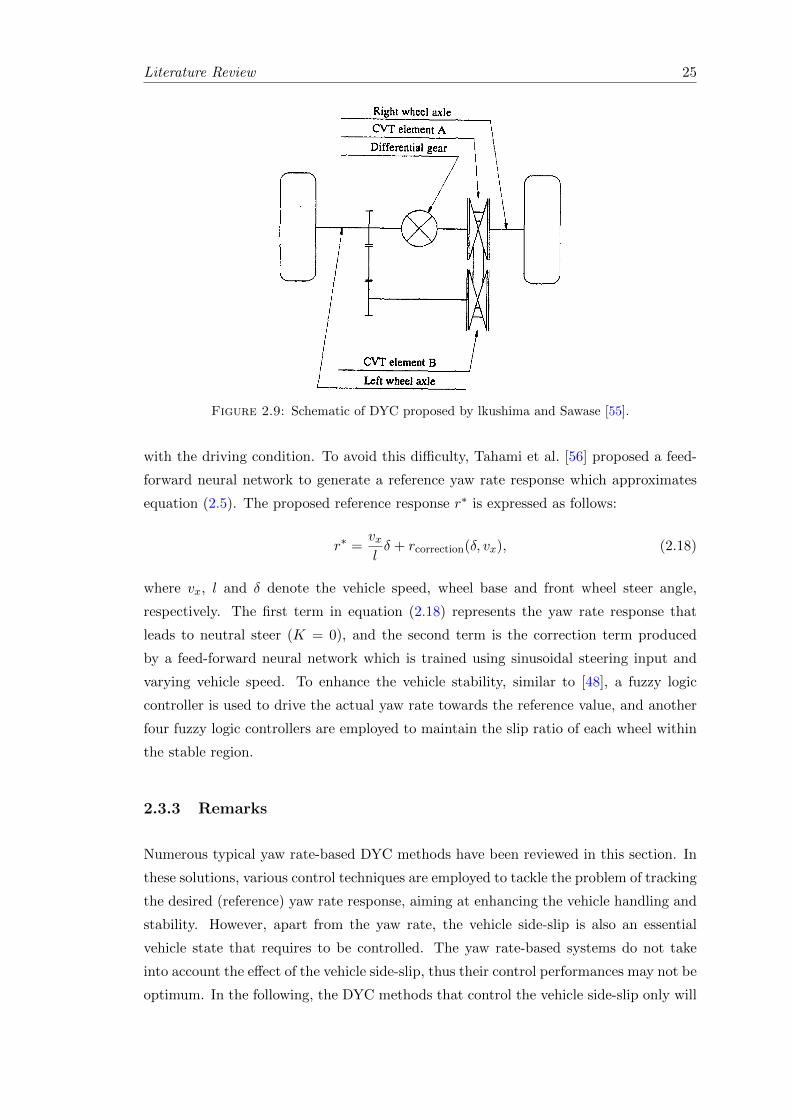
Literature Review 25
When yaw moment control is not required, themechanism is in a state as shown in Fig.5(a). As thesame compressive force is applied onto CVTelements A and B, with the right and left wheelsrotating freely and the CVT belt not slipping, theinput torque (Tin) is distributed to the right and leftwheels equally. The CVT is working at a velocityratio(ρ) as determined by the difference in rotatingspeed between the right and left wheels as thevehicle is cornering.
When a clockwise yaw moment is required, themechanism will change states to that shown inFig.5(b). As the compressive force on CVT elementA is increased, a force is generated to raise the gearvelocity ratio(ρ), raising the torsion in the torque
transfer shaft. Torque is then transferred from theright wheel axle to the left wheel axle. For thetorque( ΔT) transferred through the CVT to the leftwheel axle, the resultant torque on the right wheelaxle(TR) becomes:
On the other hand, for the torque(ΔT) imparted tothe left wheel axle, the resultant torque on the leftwheel axle (TL) becomes:
Thus the torque on the left axle becomes larger thanon the right axle, thereby generating a clockwise yawmoment on the vehicle.
When the condition is reversed and a counterclockwise yaw moment is required, the mechanismwill change state to that shown in Fig.5(c). As thecompressive force is increased on CVT element B, aforce is generated to reduce the gear velocityratio(ρ), giving rise to atorsion in the torque transfershaft. Torque is then transferred from the left wheelaxle to the right wheel axle. For the torque(ΔT)transferred through the CVT to the right axle, theresulting torque on the right axle(TR) becomes.
On the other hand, for the torque(ΔT) absorbedfrom the left axle, the resulting torque on left axle(TL) becomes:
Thus the torque on the right axle becomes largerthan on the left axle, thereby, generating a counterclockwise yawmoment on the vehicle.
4
Downloaded from SAE International by Brought to you by RMIT University, Thursday, June 19, 2014
Figure 2.9: Schematic of DYC proposed by lkushima and Sawase [55].
with the driving condition. To avoid this difficulty, Tahami et al. [56] proposed a feed-
forward neural network to generate a reference yaw rate response which approximates
equation (2.5). The proposed reference response r∗ is expressed as follows:
r∗ =vxlδ + rcorrection(δ, vx), (2.18)
where vx, l and δ denote the vehicle speed, wheel base and front wheel steer angle,
respectively. The first term in equation (2.18) represents the yaw rate response that
leads to neutral steer (K = 0), and the second term is the correction term produced
by a feed-forward neural network which is trained using sinusoidal steering input and
varying vehicle speed. To enhance the vehicle stability, similar to [48], a fuzzy logic
controller is used to drive the actual yaw rate towards the reference value, and another
four fuzzy logic controllers are employed to maintain the slip ratio of each wheel within
the stable region.
2.3.3 Remarks
Numerous typical yaw rate-based DYC methods have been reviewed in this section. In
these solutions, various control techniques are employed to tackle the problem of tracking
the desired (reference) yaw rate response, aiming at enhancing the vehicle handling and
stability. However, apart from the yaw rate, the vehicle side-slip is also an essential
vehicle state that requires to be controlled. The yaw rate-based systems do not take
into account the effect of the vehicle side-slip, thus their control performances may not be
optimum. In the following, the DYC methods that control the vehicle side-slip only will
Literature Review 26
be first reviewed, followed by the introduction to more comprehensive and sophisticated
DYC solutions which regulate both the yaw rate and vehicle side-slip simultaneously.
2.4 VEHICLE SIDE-SLIP-BASED DYC
2.4.1 Background
As introduced in Chapter 1, in addition to the yaw rate r, the vehicle side-slip β is
also an essential vehicle state that needs to be controlled. Ideally, the vehicle side-slip
requires to be minimized for two reasons. Firstly, according to the findings reported
in [21], when the vehicle side-slip increases to large values, the tire cornering stiffnesses
decrease and the yaw moment generated by the lateral tire forces descends. Since the
slopes of the yaw moment curves (see Fig. 5 in [21]) are close to zero, the generated
yaw moment can hardly be increased by changing the steer angle. This means that no
sufficient yaw moment can be generated at large vehicle side-slip, which may lead the
vehicle to lose its stability. Secondly, a small vehicle side-slip indicates a consistency
of the vehicle heading direction with the velocity vector v (shown in Figure 1.4). This
consistency provides the driver with superior sense of control during cornering [22], as
the driver intuitively assumes that the vehicle heading direction is the direction where
the vehicle is going. Due to these reasons, zero desired vehicle side-slip, β∗ = 0, is often
employed in the vehicle dynamics and control literature.
Note that β∗ = 0 is a strict condition to be satisfied. Indeed, many existing DYC solu-
tions aim to limit β in a stable region or control β to follow some prescribed dynamics,
in order to prevent it from diverging and maintain the vehicle stability. For example, the
steady-state vehicle side-slip response (or its variation/modification) derived from the
two DoF planar vehicle model [20] is often employed as the desired (reference) vehicle
side-slip. This value can be expressed in the following general form [35]:
β =
(lr −
mlfv2x
lCαr
)δ
l(1 +Kv2x), (2.19)
where the symbols used are consistent with those in equation (2.5).
In the following section, the typical vehicle side-slip-based DYC solutions are reviewed.
These methods either constrain β in a stable region, or track a desired (reference) re-
sponse, i.e. zero vehicle side-slip or equation (2.19) (or its variation/modification). Note

Literature Review 27
that apart from the vehicle side-slip-based DYC systems for electric vehicles with inde-
pendent motors, other typical types of vehicle side-slip-based DYC methods (e.g. dif-
ferential braking systems) are also reviewed, as they share similar design principles and
lay the foundation for new DYC designs.
2.4.2 Typical vehicle side-slip-based DYC methods
Abe et al. [57] proposed a DYC control method employing zero desired vehicle side-slip,
β∗ = 0. In this design, the transfer function of the vehicle side-slip response with the
DYC system on-board is expressed as follows:
β(p) =Bf (p)δ(p) +BMM(p)
G(p), (2.20)
where p denotes the Laplace transform variable, β(p), δ(p) and M(p) are the Laplace
transformations of the vehicle side-slip, steering wheel angle and corrective yaw moment
generated by the DYC, respectively, and Bf (p), BM and G(p) are coefficients expressed
by the vehicle parameters (see [57]). Setting this vehicle side-slip response to zero leads
to the following control law:M
δ(p) = − Bf
BM(p). (2.21)
Comparative simulation results indicate that the proposed DYC is less effective than
4-Wheel-Steering (4WS) in achieving zero vehicle side-slip, but it provides a more re-
sponsive yaw rate response than 4WS.
To analyze the vehicle stability graphically, a phase-plane method considering two vehicle
states (vehicle side-slip β and its derivative β) is proposed by Inagaki et al. [58]. In view
of the fact that the vehicle stability is intrinsically related to the vehicle lateral motion,
this method plots the state trajectories of the vehicle system on the β − β phase-plane.
The stable and unstable regions, as well as how the trajectories evolve with time, are
clearly portrayed on the phase-plane, which provides insights into how vehicle stability
control systems should be designed to keep the vehicle stable. The state trajectories are
kept in the stable region if the following condition is satisfied:
|C1β + C2β| < 1, (2.22)
where C1 and C2 are two constants.
Based on this method, different DYC systems (e.g. [58–63]) have been devised to achieve
the task of maintaining the vehicle state trajectories within the stable region. Yasui et
al. [61] designed a vehicle stability enhancement system to achieve this task by controlling
Literature Review 28
the wheel slip ratio of the front-outer wheel. The target wheel slip ratio is defined as
follows:
λ∗ = K1β +K2β, (2.23)
where K1 and K2 are two design parameters. The brake pressure for the front-outer
wheel is regulated to track this desired wheel slip ratio so that the state trajectories
remain in the stable region. In the work of Tian et al. [62], when the point (β, β) on
the phase-plane is outside the stable region, a DYC system is activated to drive it back
to the stable region. The nearest distance between the point (β, β) and the boundary
of the stable region is defined as d. A simple PI controller is employed by the DYC to
drive d to zero, with the distance d being the input and the corrective yaw moment M
being the output. When the point (β, β) is inside the stable region, an AFS system
based on sliding mode control is adopted to track the response of a reference vehicle
model. An analogous DYC approach which also adopts the distance d to determine the
control effort is proposed by He et al. [63].
Uematsu and Gerdes [17] proposed a sliding mode control scheme that employs the
vehicle side-slip and its derivative in the sliding surface design. This sliding surface can
be written as:
s = β + αβ = 0, (2.24)
where α is a positive design parameter. To drive the state trajectory towards the sliding
surface, the following sliding condition should be satisfied:
s = −ks, (2.25)
where k represents the convergence rate at which the state trajectory approaches the
sliding surface. It should be pointed out that this control design faces an implementation
challenge as the control input requires the derivatives of the lateral tire forces due to
the involvement of β in the sliding surface.
Furukawa and Abe [64, 65] devised a DYC strategy to regulate the vehicle side-slip in
conjunction with 4WS by means of sliding mode control. In this design, the vehicle
states are driven towards the sliding surface defined as follows:
s = β + c(β + aβ) = 0, (2.26)
where a and c are two design parameters. To guarantee that the above sliding surface
is reached, the following sliding condition is mandated:
s = −ks, (2.27)
Literature Review 29
where k denotes the convergence rate. The information of β required to generate the
control command is estimated by integrating the lateral tire forces computed from an
on-board tire model. When the control strategy is applied to a 2-Wheel-Steering (2WS)
vehicle, the sliding surface is modified as follows:
s = β + c(β − β∗) = 0, (2.28)
where β∗ is the steady-state vehicle side-slip response expressed by equation (2.19).
In the works of Abe et al. [66–68], a model following control by means of sliding mode
control is proposed to compensate for the loss of stability due to the nonlinear tire
characteristics. The model response to be followed is derived from the common two
DoF planar vehicle model (bicycle model), and it can be expressed in the form of a
transfer function as follows:
β
δ(p) = G
1 + Tp
1 +Q
Pp+
1
Pp2, (2.29)
where p denotes the Laplace transform variable, G is the vehicle side-slip gain constant
(the value of β in response to δ in steady state), and T , Q and P are constants expressed
by the vehicle parameters (see [66]). A sliding mode controller is adopted for the model
following control. The sliding surface is achieved by rewriting equation (2.29) in the
following form:
s = β +Qβ + Pβ − PGT δ − PGδ = 0. (2.30)
The sliding condition to be satisfied is written as:
s = −ks, (2.31)
where k represents the convergence rate. By this means, the vehicle side-slip response
is controlled to follow the model response expressed by equation (2.29), which in turn
enhances the vehicle stability. Abe et al. [66] concluded that: the vehicle side-slip-based
DYC is more effective than the yaw rate-based DYC and 4WS in stabilizing the vehicle.
2.4.3 Remarks
The implementation of the vehicle side-slip-based DYC schemes requires the real-time
information of the vehicle side-slip angle β, therefore a properly designed state observer
is necessary to estimate this state as no standard sensors are available for low-cost mea-
surements. The estimation of β is outside the scope of this study, but it has become
Literature Review 30
a research focus and numerous estimation methods have been proposed in the litera-
ture [69–74].
So far, the typical control methods that regulate the yaw rate only and the vehicle
side-slip only have been reviewed in two seperate sections. Even though the yaw rate
and vehicle side-slip are intrinsically related by the vehicle dynamics (see the vehicle
equations of motion in Chapter 3), controlling only one of them may not lead to optimum
dynamic performance in terms of the vehicle handling and stability. Indeed, integrated
control of both vehicle states has been shown to be generally more effective. In the
following, the more comprehensive and sophisticated DYC solutions that regulate both
the yaw rate and vehicle side-slip simultaneously are reviewed.
2.5 SIMULTANEOUS CONTROL OF YAW RATE AND
VEHICLE SIDE-SLIP
2.5.1 Background
As introduced in Chapter 1, the yaw rate and vehicle side-slip are known to be the two
fundamental states that govern the vehicle handling and stability. It has been pointed
out in the literature that controlling one state only may bring about problems in some
certain circumstances. For instance, on low friction roads, controlling the yaw rate only
may be insufficient to prevent the vehicle side-slip from diverging, and in turn the vehicle
may lose its stability and spin [17–19]. On the other hand, controlling the vehicle side-slip
only guarantees the vehicle stability but may not produce desirable yaw rate response
(i.e. favorable steer characteristic) [24]. As a result, in order to eliminate the downsides
resulting from controlling one state only and combine the benefits of controlling the yaw
rate and vehicle side-slip individually, numerous recent DYC works adopt both states
simultaneously as the control variables. These solutions have presented superior control
performance to the systems controlling one state only [17, 23–26].
2.5.2 Typical control methods
Sliding mode control provides robustness against system uncertainties and external dis-
turbances [75–77]. Thanks to this property, sliding mode control is ideal for controlling
nonlinear plants such as the vehicle systems, and it has been commonly adopted in the
recent DYC system designs. One critical step in designing a sliding mode controller
is the choice of switching function (thus sliding surface). The most common switching
Literature Review 31
function design in the recent DYC systems employs a linear combination of the yaw rate
and vehicle side-slip errors, which takes the following general form [17, 23, 24, 78–81]:
s = r − r∗ + ξ(β − β∗), (2.32)
where r∗ and β∗ are the desired (reference) yaw rate and vehicle side-slip, respectively,
and ξ is a positive design parameter. Both the yaw rate and vehicle side-slip errors are
adopted in this switching function, hence both vehicle states, the yaw rate and vehicle
side-slip, are regulated simultaneously by the sliding mode controller.
Yi et al. [23] devised a differential braking strategy for vehicle stability control. The
corrective yaw moment generated from differential braking is derived by means of sliding
mode control using a three DoF planar vehicle model. The proposed sliding mode
controller employs equation (2.32) as the switching function. Zero desired vehicle side-
slip, β∗ = 0, is employed in this scheme. To allow for the tire-road friction limit, the
desired (reference) yaw rate r∗ is defined as follows:
r∗ =
rt if |rt| <µg
vx,
µg
vxsgn(rt) if |rt| >
µg
vx,
(2.33)
where µ represents the friction coefficient, g denotes the gravitational acceleration and
rt is the same yaw rate response as described by equation (2.5).
The switching function, equation (2.32), was utilized by Li and Cui [78] to devise a
sliding mode controller for an electric vehicle with four independent driving wheels. The
desired yaw rate r∗ is the same as [23], while the desired vehicle side-slip is defined as
follows:
β∗ = (lrvx− lfmvx
l)r∗. (2.34)
This desired vehicle side-slip value is indeed the same as equation (2.19). In this design,
the front and rear motor torques are maintained at a fixed ratio, thereby eliminating
the task of motor torque distribution between the four driving wheels. However, this
simplified scheme does not make proper use of the adhesion condition of individual
wheels, thus it may not achieve optimum control performance. To tackle this problem,
some works have been proposed in the literature to dynamically and effectively distribute
the longitudinal tire forces to obtain a certain corrective yaw moment [82, 83].
Tchamna and Youn [24] proposed a braking-based sliding mode DYC design considering
the vehicle longitudinal dynamics, with equation (2.32) chosen as the switching function.
The feature of this design lies in that it does not adopt the simplifying assumptions
such as constant vehicle longitudinal velocity and small vehicle side-slip angle. These
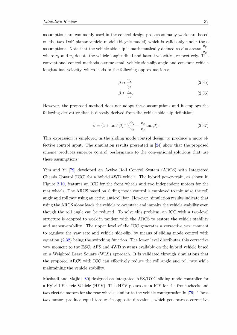
Literature Review 32
assumptions are commonly used in the control design process as many works are based
on the two DoF planar vehicle model (bicycle model) which is valid only under these
assumptions. Note that the vehicle side-slip is mathematically defined as β = arctanvyvx
,
where vx and vy denote the vehicle longitudinal and lateral velocities, respectively. The
conventional control methods assume small vehicle side-slip angle and constant vehicle
longitudinal velocity, which leads to the following approximations:
β ≈ vyvx
(2.35)
β ≈ vyvx. (2.36)
However, the proposed method does not adopt these assumptions and it employs the
following derivative that is directly derived from the vehicle side-slip definition:
β = (1 + tan2 β)−1(vyvx− vxvx
tanβ). (2.37)
This expression is employed in the sliding mode control design to produce a more ef-
fective control input. The simulation results presented in [24] show that the proposed
scheme produces superior control performance to the conventional solutions that use
these assumptions.
Yim and Yi [79] developed an Active Roll Control System (ARCS) with Integrated
Chassis Control (ICC) for a hybrid 4WD vehicle. The hybrid power-train, as shown in
Figure 2.10, features an ICE for the front wheels and two independent motors for the
rear wheels. The ARCS based on sliding mode control is employed to minimize the roll
angle and roll rate using an active anti-roll bar. However, simulation results indicate that
using the ARCS alone leads the vehicle to oversteer and impairs the vehicle stability even
though the roll angle can be reduced. To solve this problem, an ICC with a two-level
structure is adopted to work in tandem with the ARCS to restore the vehicle stability
and maneuverability. The upper level of the ICC generates a corrective yaw moment
to regulate the yaw rate and vehicle side-slip, by means of sliding mode control with
equation (2.32) being the switching function. The lower level distributes this corrective
yaw moment to the ESC, AFS and 4WD systems available on the hybrid vehicle based
on a Weighted Least Square (WLS) approach. It is validated through simulations that
the proposed ARCS with ICC can effectively reduce the roll angle and roll rate while
maintaining the vehicle stability.
Mashadi and Majidi [80] designed an integrated AFS/DYC sliding mode controller for
a Hybrid Electric Vehicle (HEV). This HEV possesses an ICE for the front wheels and
two electric motors for the rear wheels, similar to the vehicle configuration in [79]. These
two motors produce equal torques in opposite directions, which generates a corrective
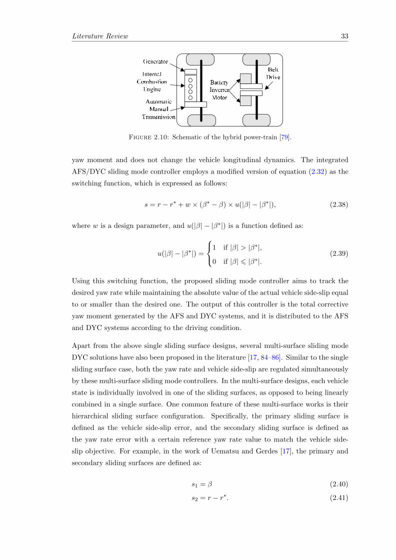
Literature Review 33
��
�
��
����������������������� ���� �������������������� �������� ��� ���� ��� �� ������� ��� �� �� �� �� ������� ��� ���������������������� !����������������"�#��$��������� ����� ���� � ������������� % ��$���������������������������������� ����!� ������� ����������������$������� ��� ����%������ �� ��� � ������ !� �� ����&� ���� ���� "�#�� ���������$�"�#������� ���������� ��� ��������%� ������������������� � �� �� ������ ��� !���&� ��� ��� '%����� !� ���� ������� ���� ����� �����(���&�� ������� �� �������)������� !����������*+�$�+��� ��!����� ���� �����+,������%��� ����� ����� �����!����� $�*��� ���� ��'%���*-���������%� ��� ������ ���. �������������� ����� ���% � ����� �����!����� $����%� �����������������%� ������� !�&������/&����!� � � ���������������!� ������������ �������"�#$�
��� ������������ ���������� ������������������������������������ ���!���
���� "� �����!������ ��#���������� ��!������� ��������#����� ������������ �#������ �$������� ����"���� ��� �" �� ��� ��������� ������������������ ��!����%&'������������������� ���������(�������� ������"� ��������������)� �������� ��#� �������������� ���������)���������������� �"���������� ������"� ����������������!!� �������� ���������#�������"� �*�����*����� �� ����������������� ������ ����*� ��� � ����� ����)����� ���� ��� ����� �!!� ����� ��� ���������#� ���� �������������!� ������ ��� %+'�� ��� ����� � ��*� ���� ���������)��������������� ����������� �"�����!���������
��������������������������������!�������#���#��� ����������!��� ����� �" �� ��� (���� ���� �������� � ���������)������ ,� ������� %-'*� ./0).��� ������� %1'*� ���� #���)� ���"���� ��� ������� %2'*� �� �� ��� ����� � ��*� ���� ������#� ����� ������� ������ ���� �������#���� ���������� !���������� �"��� ��� ������ ������� �(��!"����
3��� ����#���#� �� ���������� !��� ����*� ��� ��� �� ������� �������"��� ��� ��������� ���� ����� ��#��� ���� ���� ����� ������ 3��� ����� "� ���*� �������� �������� ����� ����� �� ����� %4'�� 5���� �!������������� ������������ ������ �����)��� �����������6�(����*���� ��� ��!!� "��� ��� ����"��� ���� ����� ����� ��� ���� ����� ��#"����� ���������� ��� ���������#� ���� ����� ��#���� � ��� ����� � ��*� ���� ��)��� � ��������� ����� ��� ������� ��� ���� ����"���� ��������� ���������������� ����%7'���
���� �� ���������������������� �������8������ �������������� ��� �$������ ��� ����)������ ���� ������� �� ��� �� ���"��*� ���� ���������� ���� ��� ��� ���!����� ����� ������ ���� ����� �!� ��������"������������ ��� ��������� ���� ����"����������*� ����
���9�������:��9������(��������� ���������"�����!�������#�� ���� �����#�*����� ���� � ����� �!� 5� ���� ��� ���� ����� � �� ;�#�������#*� ���"�� ������������������*����"�*� &2&)711*�:����*� ��� � ������� ��)����<���(���=������ ��>�8��=��"�� �8����
����#������ ������� ������� ������ (���� ;��*� �3�*� ���� 1?�(�� �������������������61@����� �� �������
���������������(���� ����*������#�����"����!������� �������������� ������ !����������������� ��� ������� ���� �6;@������������� ������� �"��� ��� ����� ������ ����*� �������� ��!�#"������������������ �� ������������#���#�6;@���" �����������*� ������������ �������� ��!�#"��������%A'������#��������� ����!�6;@�*����������1?����� ����61@�������#���� ���������!�������!"���� ������ ���� ���� ���� ��� ������� �������� 3�#�� &� ���(�� ���� ��!�#"��������!�����61@*������� ������5����%B*&C'��D������������������#����" ���������������E��� ����������������� ��� ������"��*� �����(��#��� �������"����*� ���� ���� ��� ����� � 8�#��#*����� � ���������!��������� ��� ������� ������� ��������#��!� �������� ������ ��� �������#� ;��*� �3�� ���� 1?*� (�� �� ��� ������������������� ������������)������������(���������61@��
�
�3�#��&�� ������ ����(��!�����61@�������� �(��)������
����� !���61@�� ���� �(�)������ ���" �"��<� ��� " ��)������ ����
��(��)������ ����������� ��� ���� " ��)������ ���������*� �� ���� ����(� ������� ������� ��� � ����� ��� #�������� �� ������� ��(�������� (�� �� ��� ������� ��� �������E�� �� ���� ���� ��� ������(��)������ ���������*� ���� ������� ��(�������� ����������"����"���#� ?.�� (���� ;��*� �3�*� ���� 1?�� ?.�� ��� �� #���� ����������� �"������ ������������� ������������������������"#������ ��#����� � �� "������� %&&*&+'�� ��� �� ������� ���� � �"����� ��!�#"��������!�;��������3�� ���?.��!���"������*����������(��#����#���!�������F� �����!"� ��������?.������ �� ��������� �� 8������!!� ����������!����� �� �����������*����"������������ ��!��������������� ������"������� � 8�#���������%&-'��
����� � ��������#���E������!����(�<������ �����+*����� ���������� ���������������������#����(����������#������ ����������������&)�3�����������*��������"������������ ��!������������ �����-*������� ����(�������� �����������������#����(��������������� � ��������*�������(���������������"������ ���������������?.��(�������������(��#����#����� ��������������� �����1*����"������������ ��!���������������������� �� �"����������#���������� �����2��
���� ;��0���3�����@;���..�������.��9��;5����&����#���!��� ����������!���� ���������)���������
+���������� ����������� ������� ������� �� ������������ ��������"�������*+�#������
����#F���9�������:���#�"�9��
2011 14th International IEEE Conference onIntelligent Transportation SystemsWashington, DC, USA. October 5-7, 2011
978-1-4577-2197-7/11/$26.00 ©2011 IEEE 1193
Figure 2.10: Schematic of the hybrid power-train [79].
yaw moment and does not change the vehicle longitudinal dynamics. The integrated
AFS/DYC sliding mode controller employs a modified version of equation (2.32) as the
switching function, which is expressed as follows:
s = r − r∗ + w × (β∗ − β)× u(|β| − |β∗|), (2.38)
where w is a design parameter, and u(|β| − |β∗|) is a function defined as:
u(|β| − |β∗|) =
1 if |β| > |β∗|,0 if |β| 6 |β∗|.
(2.39)
Using this switching function, the proposed sliding mode controller aims to track the
desired yaw rate while maintaining the absolute value of the actual vehicle side-slip equal
to or smaller than the desired one. The output of this controller is the total corrective
yaw moment generated by the AFS and DYC systems, and it is distributed to the AFS
and DYC systems according to the driving condition.
Apart from the above single sliding surface designs, several multi-surface sliding mode
DYC solutions have also been proposed in the literature [17, 84–86]. Similar to the single
sliding surface case, both the yaw rate and vehicle side-slip are regulated simultaneously
by these multi-surface sliding mode controllers. In the multi-surface designs, each vehicle
state is individually involved in one of the sliding surfaces, as opposed to being linearly
combined in a single surface. One common feature of these multi-surface works is their
hierarchical sliding surface configuration. Specifically, the primary sliding surface is
defined as the vehicle side-slip error, and the secondary sliding surface is defined as
the yaw rate error with a certain reference yaw rate value to match the vehicle side-
slip objective. For example, in the work of Uematsu and Gerdes [17], the primary and
secondary sliding surfaces are defined as:
s1 = β (2.40)
s2 = r − r∗. (2.41)
Literature Review 34
In order to achieve the primary control objective – zero vehicle side-slip, considering the
two DoF planar vehicle model, the following desired yaw rate must be tracked:
r∗ =
∑Fy
mvx− β, (2.42)
where∑Fy denotes the total external forces acted on the vehicle in the lateral direction.
The limitation of this sliding surface configuration is that the desired yaw rate in the
secondary surface has to be a certain function, and cannot be assigned an arbitrary
reference value as in the single-surface case. In other words, the yaw rate and vehicle side-
slip cannot actually be independently controlled. Comparative simulations presented
in [17] show that both the single-surface and multi-surface schemes present superior
control performances to the systems employing only one vehicle state as the control
variable. In particular, the multi-surface system provides better robustness but slower
yaw rate response than the single-surface scheme.
Even though sliding mode control has become the most popular control technique in the
recent DYC solutions for regulating the yaw rate and vehicle side-slip simultaneously,
other typical types of control techniques are also employed in the literature to tackle the
same problem. Chumsamutr and Fujioka [87] proposed a DYC scheme based on optimal
control theory to control the driving and braking torques for an electric vehicle. The
two DoF planar vehicle model used in the proposed design can be expressed with the
following state-space representation:
x = Ax+BM +Eδ, (2.43)
where x = [β r]T denotes the state vector, M represents the corrective yaw moment,
δ stands for the front wheel steer angle, and A, B and E are the coefficient matrices
expressed by the vehicle parameters (see [87]). The steady-state responses of β and r
derived from the two DoF model with M = 0 are taken as the desired responses, denoted
by xdes. Then, the vehicle dynamics in terms of the error vector e = x−xdes is described
as:
e = Ae+BM. (2.44)
The corrective yaw moment M is determined in such a way that the following cost
function is minimized:
J =
∫ ∞
0
(eTQe+ εM2
)dt, (2.45)
where ε is a design parameter and Q is a design matrix. The simulation results indicate
that in the linear region of the tire characteristics, the proposed controller provides the
vehicle with a faster cornering response, while in the nonlinear region, the controller
ensures the vehicle stability by driving the vehicle side-slip close to zero. Several similar
Literature Review 35
control approaches have also been proposed [1, 88–92] to regulate the yaw rate and
vehicle side-slip simultaneously by means of optimal control theory.
Fuzzy logic control techniques are also employed by DYC systems to regulate both the
yaw rate and vehicle side-slip, as fuzzy logic control provides the benefit of not requiring
a mathematical model of the plant while still being highly robust [25]. Zhao et al. [93]
proposed a DYC solution based on fuzzy logic control for a four-in-wheel-motor drive
electric vehicle. In this design, equation (2.5) is used as the desired yaw rate response
and zero vehicle side-slip is adopted as the desired vehicle side-slip response. The inputs
to this fuzzy logic controller are the yaw rate error and vehicle side-slip error, and the
output from this controller is the corrective yaw moment. This control scheme is proven
to be effective in controlling the yaw rate and vehicle side-slip by both simulations and
experiments. A similar fuzzy logic control approach to the above solution is available in
the work of Kim et al. [94].
Buckholtz [26] devised a fuzzy logic yaw rate control scheme with vehicle side-slip limita-
tion. This fuzzy logic controller tracks the desired yaw rate by assigning an appropriate
wheel slip ratio to each wheel. The yaw rate tracking is activated only when the error
quantity, e = r∗ − r + k(r∗ − r) (k > 0 is a design parameter), exceeds a user-defined
threshold. Using this indirect approach, the vehicle side-slip magnitude is restricted and
no information of the vehicle side-slip is required.
In the work of Sun et al. [95], a fuzzy logic control algorithm is developed to integrate
the DYC and AFS. This fuzzy logic controller produces control commands for the DYC
and AFS to track the desired yaw rate and vehicle side-slip simultaneously. The two
inputs to the fuzzy logic controller are the yaw rate and vehicle side-slip errors, and the
outputs from this controller are the corrective yaw moment generated by the DYC and
the corrective front wheel steer angle produced by the AFS.
2.5.3 Remarks
Aiming at eliminating the downsides resulting from controlling one state only and com-
bining the benefits of controlling the yaw rate and vehicle side-slip individually, numerous
DYC solutions have been proposed in the recent literature to regulate both states simul-
taneously. In this section, typical DYC systems of such type have been reviewed. For
each DYC control scheme, the theories and principles behind the control technique are
clearly explained. Note that sliding mode control has become the most prevalent control
technique in this field due to its robustness against disturbances and uncertainties for
controlling nonlinear systems. Different variations of sliding mode DYC schemes, for
example various sliding surface designs, are currently being extensively discussed in the
Literature Review 36
literature. The implementations of these sliding mode controllers require real-time infor-
mation of the yaw rate and vehicle side-slip, which necessitates the design of appropriate
measuring and/or estimation methods. Besides, more experimental results are needed
to comprehensively and thoroughly validate the effectiveness of these sliding mode DYC
approaches.
Chapter 3
Full Vehicle Model
To validate the DYC designs proposed in the subsequent chapters through compre-
hensive computer simulations, an accurate full vehicle model that reflects closely the
vehicle dynamics in reality is required to establish the simulation model in the MAT-
LAB/Simulink environment. The vehicle equations of motion, as part of the full vehicle
model, are the mathematical representation of the plant (i.e. the vehicle) and they ex-
press the dynamics of the vehicle longitudinal motion, lateral motion, roll motion and
yaw motion. These equations are required in the subsequent chapters for control system
design. For these reasons, a full vehicle model, including the vehicle equivalent mechan-
ical model, vehicle equations of motion, wheel equation of motion and Magic Formula
tire model, is introduced in this chapter.
3.1 VEHICLE EQUIVALENT MECHANICAL MODEL
In order to obtain the vehicle equations of motion, we must first establish a vehicle
equivalent mechanical model. As a vehicle consists of two major parts: sprung mass
and unsprung mass, we regard these two parts as two rigid bodies in the mechanical
model. Figure 3.1 shows the vehicle equivalent mechanical model and the attached
coordinate systems. This mechanical model consists of two rigid bodies, with the top
body denoting the vehicle sprung mass and the bottom one representing the unsprung
mass. The coordinate system x-y-z is attached to the unsprung rigid body. The origin
of the coordinate system, P, is right under the mass center of the entire vehicle when the
vehicle is stationary. The x axis coincides with the vehicle longitudinal direction, the
y axis goes laterally to the left from the driver’s view, and the z axis directs vertically
upwards. The other coordinate system x′-y′-z′ is fixed to the sprung rigid body with
the same origin P. When the vehicle is stationary, the two coordinate systems coincide.
37
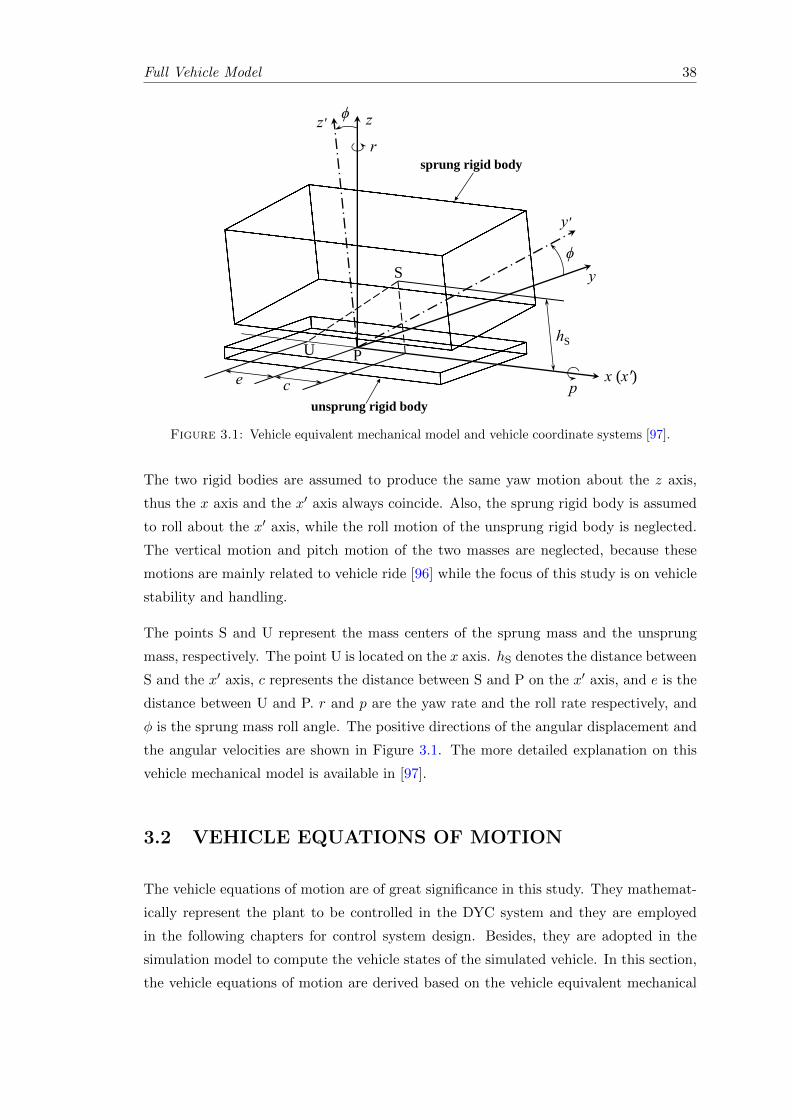
Full Vehicle Model 38
ϕ
ϕ
r
zz'
y
y'
hS
px (x')
S
U P
ce
sprung rigid body
unsprung rigid body
Figure 3.1: Vehicle equivalent mechanical model and vehicle coordinate systems [97].
The two rigid bodies are assumed to produce the same yaw motion about the z axis,
thus the x axis and the x′ axis always coincide. Also, the sprung rigid body is assumed
to roll about the x′ axis, while the roll motion of the unsprung rigid body is neglected.
The vertical motion and pitch motion of the two masses are neglected, because these
motions are mainly related to vehicle ride [96] while the focus of this study is on vehicle
stability and handling.
The points S and U represent the mass centers of the sprung mass and the unsprung
mass, respectively. The point U is located on the x axis. hS denotes the distance between
S and the x′ axis, c represents the distance between S and P on the x′ axis, and e is the
distance between U and P. r and p are the yaw rate and the roll rate respectively, and
φ is the sprung mass roll angle. The positive directions of the angular displacement and
the angular velocities are shown in Figure 3.1. The more detailed explanation on this
vehicle mechanical model is available in [97].
3.2 VEHICLE EQUATIONS OF MOTION
The vehicle equations of motion are of great significance in this study. They mathemat-
ically represent the plant to be controlled in the DYC system and they are employed
in the following chapters for control system design. Besides, they are adopted in the
simulation model to compute the vehicle states of the simulated vehicle. In this section,
the vehicle equations of motion are derived based on the vehicle equivalent mechanical
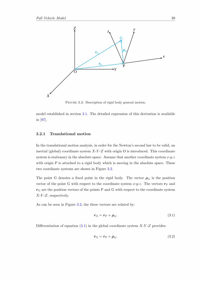
Full Vehicle Model 39
x
z y
PO
X
Y
Z
rP
rGρG
G
Figure 3.2: Description of rigid body general motion.
model established in section 3.1. The detailed expression of this derivation is available
in [97].
3.2.1 Translational motion
In the translational motion analysis, in order for the Newton’s second law to be valid, an
inertial (global) coordinate system X-Y -Z with origin O is introduced. This coordinate
system is stationary in the absolute space. Assume that another coordinate system x-y-z
with origin P is attached to a rigid body which is moving in the absolute space. These
two coordinate systems are shown in Figure 3.2.
The point G denotes a fixed point in the rigid body. The vector ρG is the position
vector of the point G with respect to the coordinate system x-y-z. The vectors rP and
rG are the position vectors of the points P and G with respect to the coordinate system
X-Y -Z, respectively.
As can be seen in Figure 3.2, the three vectors are related by:
rG = rP + ρG. (3.1)
Differentiation of equation (3.1) in the global coordinate system X-Y -Z provides:
rG = rP + ρG. (3.2)
Full Vehicle Model 40
Expressing the vector ρG in the coordinate system x-y-z and applying the Transport
Theorem in mechanics [98] lead to:
ρG = ρGrel + ω × ρG, (3.3)
where ρGrel represents the relative velocity of the point G with respect to the coordinate
system x-y-z, and ω denotes the angular velocity of the coordinate system x-y-z with
respect to the coordinate system X-Y -Z. In this study ρGrel = 0 since the point G is
fixed in the coordinate system x-y-z. Note that rP, the velocity of the point P with
respect to the coordinate system X-Y -Z, should be expressed in the coordinate system
x-y-z in order for the addition in equation (3.2) to be valid. Substituting equation (3.3)
in equation (3.2) gives:
rG = rP + ω × ρG. (3.4)
Now equation (3.4) is applied to the sprung rigid body and unsprung rigid body. The
position vectors of the points S and U with respect to the coordinate system X-Y -Z
are denoted by rS and rU, respectively, the position vectors of the points S and U
with respect to the coordinate systems x′-y′-z′ and x-y-z are denoted by ρS and ρU,
respectively, and the angular velocities of the coordinate systems x′-y′-z′ and x-y-z with
respect to the coordinate system X-Y -Z are denoted by ωS and ωU, respectively. Then,
the following relations are obtained:
rS = rP + ωS × ρS (3.5)
rU = rP + ωU × ρU. (3.6)
In equations (3.5) and (3.6), rP is expressed in the coordinate systems x-y-z and x′-y′-z′
using the unit vectors in these two coordinate systems, respectively. The unit vectors in
the x, y and z directions are denoted by i, j and k, respectively, and the unit vectors
in the x′, y′ and z′ directions are denoted by i′, j′ and k′, respectively. Then, rP can
be expressed as:
rP = vxi+ vyj = vxi′ + vy(j
′ cosφ− k′ sinφ), (3.7)
where vx and vy denote the longitudinal and lateral velocities of the point P in the x and
y directions (shown in Figure 1.4), respectively. The unit vector transformations used
in equation (3.7) are elaborated in [98], and are not repeated in this thesis. Since the
sprung mass roll angle φ is normally small (so cosφ ≈ 1 and sinφ ≈ 0) [97], equation (3.7)
simplifies to:
rP = vxi+ vyj = vxi′ + vyj
′. (3.8)
Full Vehicle Model 41
It is seen from Figure 3.1 that the sprung rigid body possesses a roll angular velocity p
about the x′ axis, and a yaw angular velocity r about the z axis. In the following, p and
r will be referred to as roll rate and yaw rate, respectively. The total angular velocity of
the coordinate system x′-y′-z′ (i.e. the sprung rigid body) with respect to the coordinate
system X-Y -Z is:
ωS = pi′ + rk = pi′ + r(j′ sinφ+ k′ cosφ). (3.9)
For the same reason explained above, equation (3.9) reduces to:
ωS = pi′ + rk = pi′ + rk′. (3.10)
As the roll motion of the unsprung rigid body is neglected, the unsprung rigid body
possesses only a yaw angular velocity r about the z axis. Thus, the total angular
velocity of the coordinate system x-y-z (i.e. the unsprung rigid body) with respect to
the coordinate system X-Y -Z is:
ωU = rk. (3.11)
The position vectors ρS and ρU are expressed in the coordinate systems x′-y′-z′ and
x-y-z, respectively:
ρS = ci′ + hSk′ (3.12)
ρU = −ei. (3.13)
Substituting equations (3.8), (3.10) and (3.12) in equation (3.5), and equations (3.8),
(3.11) and (3.13) in equation (3.6) lead to:
rS = vxi′ + (vy − hSp+ cr)j′ (3.14)
rU = vxi+ (vy − er)j. (3.15)
Differentiating equations (3.14) and (3.15) in the global coordinate system X-Y -Z yields:
rS = vxi′ + vxi
′ + (vy − hSp+ cr)j′ + (vy − hSp+ cr)j′ (3.16)
rU = vxi+ vxi+ (vy − er)j + (vy − er)j. (3.17)
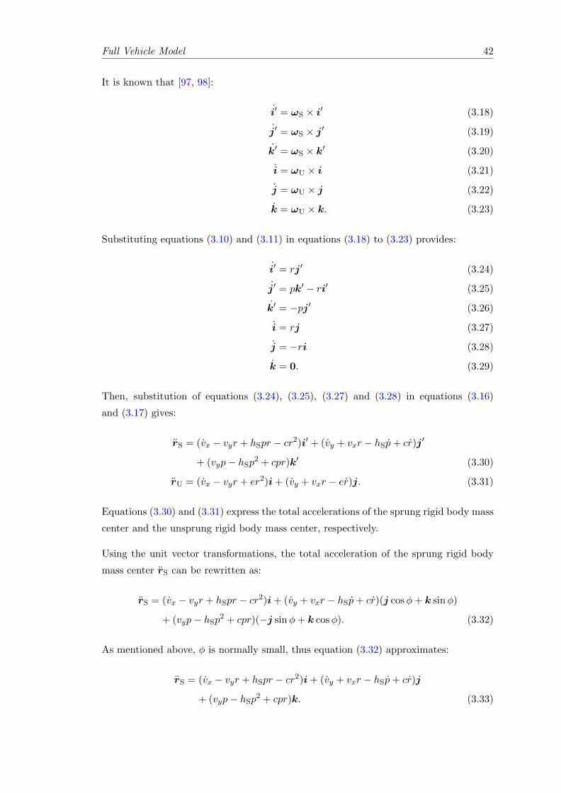
Full Vehicle Model 42
It is known that [97, 98]:
i′ = ωS × i′ (3.18)
j′ = ωS × j′ (3.19)
k′ = ωS × k′ (3.20)
i = ωU × i (3.21)
j = ωU × j (3.22)
k = ωU × k. (3.23)
Substituting equations (3.10) and (3.11) in equations (3.18) to (3.23) provides:
i′ = rj′ (3.24)
j′ = pk′ − ri′ (3.25)
k′ = −pj′ (3.26)
i = rj (3.27)
j = −ri (3.28)
k = 0. (3.29)
Then, substitution of equations (3.24), (3.25), (3.27) and (3.28) in equations (3.16)
and (3.17) gives:
rS = (vx − vyr + hSpr − cr2)i′ + (vy + vxr − hSp+ cr)j′
+ (vyp− hSp2 + cpr)k′ (3.30)
rU = (vx − vyr + er2)i+ (vy + vxr − er)j. (3.31)
Equations (3.30) and (3.31) express the total accelerations of the sprung rigid body mass
center and the unsprung rigid body mass center, respectively.
Using the unit vector transformations, the total acceleration of the sprung rigid body
mass center rS can be rewritten as:
rS = (vx − vyr + hSpr − cr2)i+ (vy + vxr − hSp+ cr)(j cosφ+ k sinφ)
+ (vyp− hSp2 + cpr)(−j sinφ+ k cosφ). (3.32)
As mentioned above, φ is normally small, thus equation (3.32) approximates:
rS = (vx − vyr + hSpr − cr2)i+ (vy + vxr − hSp+ cr)j
+ (vyp− hSp2 + cpr)k. (3.33)
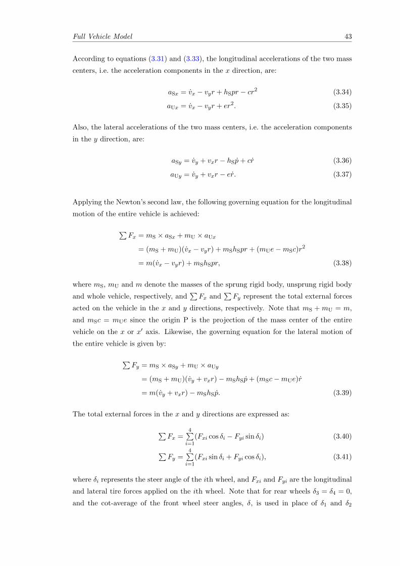
Full Vehicle Model 43
According to equations (3.31) and (3.33), the longitudinal accelerations of the two mass
centers, i.e. the acceleration components in the x direction, are:
aSx = vx − vyr + hSpr − cr2 (3.34)
aUx = vx − vyr + er2. (3.35)
Also, the lateral accelerations of the two mass centers, i.e. the acceleration components
in the y direction, are:
aSy = vy + vxr − hSp+ cr (3.36)
aUy = vy + vxr − er. (3.37)
Applying the Newton’s second law, the following governing equation for the longitudinal
motion of the entire vehicle is achieved:
∑Fx = mS × aSx +mU × aUx
= (mS +mU)(vx − vyr) +mShSpr + (mUe−mSc)r2
= m(vx − vyr) +mShSpr, (3.38)
where mS, mU and m denote the masses of the sprung rigid body, unsprung rigid body
and whole vehicle, respectively, and∑Fx and
∑Fy represent the total external forces
acted on the vehicle in the x and y directions, respectively. Note that mS + mU = m,
and mSc = mUe since the origin P is the projection of the mass center of the entire
vehicle on the x or x′ axis. Likewise, the governing equation for the lateral motion of
the entire vehicle is given by:
∑Fy = mS × aSy +mU × aUy
= (mS +mU)(vy + vxr)−mShSp+ (mSc−mUe)r
= m(vy + vxr)−mShSp. (3.39)
The total external forces in the x and y directions are expressed as:
∑Fx =
4∑i=1
(Fxi cos δi − Fyi sin δi) (3.40)
∑Fy =
4∑i=1
(Fxi sin δi + Fyi cos δi), (3.41)
where δi represents the steer angle of the ith wheel, and Fxi and Fyi are the longitudinal
and lateral tire forces applied on the ith wheel. Note that for rear wheels δ3 = δ4 = 0,
and the cot-average of the front wheel steer angles, δ, is used in place of δ1 and δ2
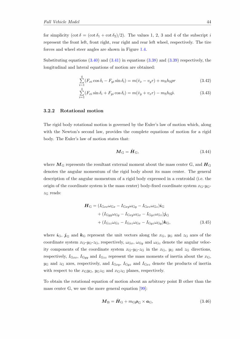
Full Vehicle Model 44
for simplicity (cot δ = (cot δ1 + cot δ2)/2). The values 1, 2, 3 and 4 of the subscript i
represent the front left, front right, rear right and rear left wheel, respectively. The tire
forces and wheel steer angles are shown in Figure 1.4.
Substituting equations (3.40) and (3.41) in equations (3.38) and (3.39) respectively, the
longitudinal and lateral equations of motion are obtained:
4∑i=1
(Fxi cos δi − Fyi sin δi) = m(vx − vyr) +mShSpr (3.42)
4∑i=1
(Fxi sin δi + Fyi cos δi) = m(vy + vxr)−mShSp. (3.43)
3.2.2 Rotational motion
The rigid body rotational motion is governed by the Euler’s law of motion which, along
with the Newton’s second law, provides the complete equations of motion for a rigid
body. The Euler’s law of motion states that:
MG = HG, (3.44)
where MG represents the resultant external moment about the mass center G, and HG
denotes the angular momentum of the rigid body about its mass center. The general
description of the angular momentum of a rigid body expressed in a centroidal (i.e. the
origin of the coordinate system is the mass center) body-fixed coordinate system xG-yG-
zG reads:
HG = (IGxxωGx − IGxyωGy − IGxzωGz)iG
+ (IGyyωGy − IGxyωGx − IGyzωGz)jG
+ (IGzzωGz − IGxzωGx − IGyzωGy)kG, (3.45)
where iG, jG and kG represent the unit vectors along the xG, yG and zG axes of the
coordinate system xG-yG-zG, respectively, ωGx, ωGy and ωGz denote the angular veloc-
ity components of the coordinate system xG-yG-zG in the xG, yG and zG directions,
respectively, IGxx, IGyy and IGzz represent the mass moments of inertia about the xG,
yG and zG axes, respectively, and IGxy, IGyz and IGxz denote the products of inertia
with respect to the xGyG, yGzG and xGzG planes, respectively.
To obtain the rotational equation of motion about an arbitrary point B other than the
mass center G, we use the more general equation [99]:
MB = HG +mGρG × aG, (3.46)
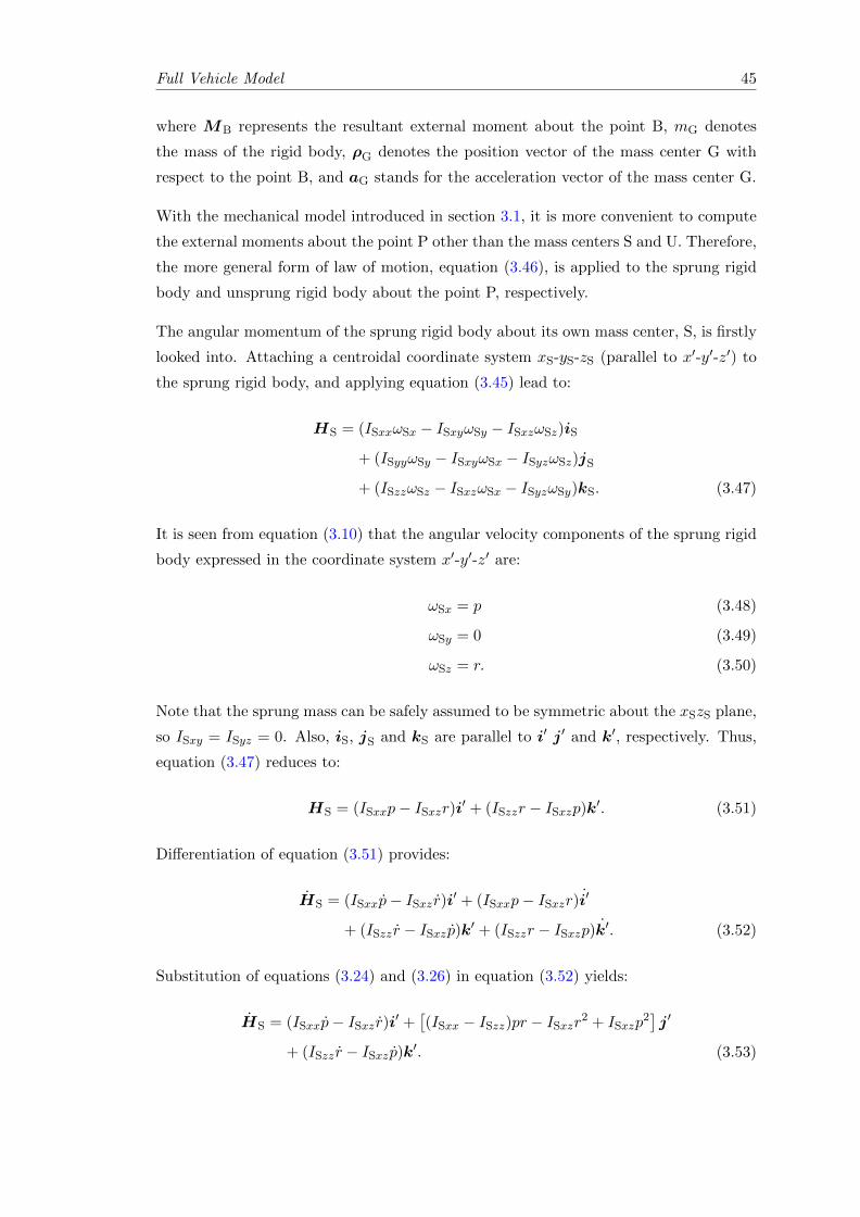
Full Vehicle Model 45
where MB represents the resultant external moment about the point B, mG denotes
the mass of the rigid body, ρG denotes the position vector of the mass center G with
respect to the point B, and aG stands for the acceleration vector of the mass center G.
With the mechanical model introduced in section 3.1, it is more convenient to compute
the external moments about the point P other than the mass centers S and U. Therefore,
the more general form of law of motion, equation (3.46), is applied to the sprung rigid
body and unsprung rigid body about the point P, respectively.
The angular momentum of the sprung rigid body about its own mass center, S, is firstly
looked into. Attaching a centroidal coordinate system xS-yS-zS (parallel to x′-y′-z′) to
the sprung rigid body, and applying equation (3.45) lead to:
HS = (ISxxωSx − ISxyωSy − ISxzωSz)iS
+ (ISyyωSy − ISxyωSx − ISyzωSz)jS
+ (ISzzωSz − ISxzωSx − ISyzωSy)kS. (3.47)
It is seen from equation (3.10) that the angular velocity components of the sprung rigid
body expressed in the coordinate system x′-y′-z′ are:
ωSx = p (3.48)
ωSy = 0 (3.49)
ωSz = r. (3.50)
Note that the sprung mass can be safely assumed to be symmetric about the xSzS plane,
so ISxy = ISyz = 0. Also, iS, jS and kS are parallel to i′ j′ and k′, respectively. Thus,
equation (3.47) reduces to:
HS = (ISxxp− ISxzr)i′ + (ISzzr − ISxzp)k′. (3.51)
Differentiation of equation (3.51) provides:
HS = (ISxxp− ISxz r)i′ + (ISxxp− ISxzr)i′
+ (ISzz r − ISxz p)k′ + (ISzzr − ISxzp)k′. (3.52)
Substitution of equations (3.24) and (3.26) in equation (3.52) yields:
HS = (ISxxp− ISxz r)i′ +[(ISxx − ISzz)pr − ISxzr2 + ISxzp
2]j′
+ (ISzz r − ISxz p)k′. (3.53)
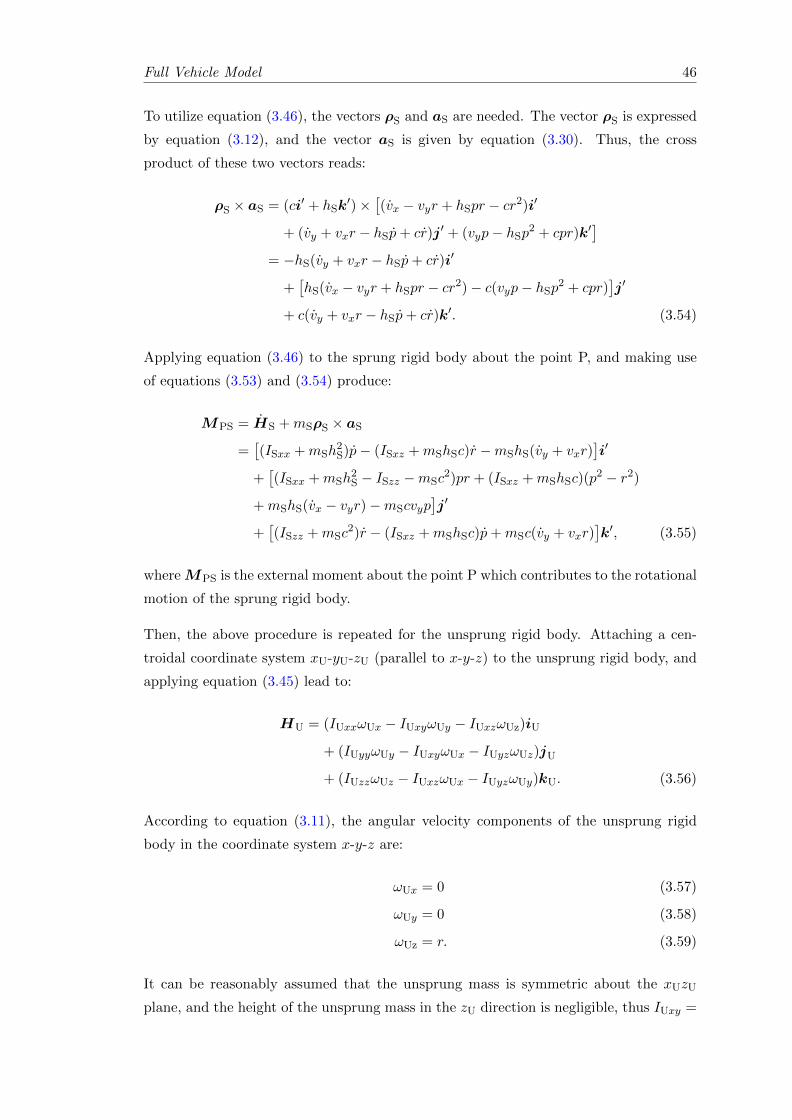
Full Vehicle Model 46
To utilize equation (3.46), the vectors ρS and aS are needed. The vector ρS is expressed
by equation (3.12), and the vector aS is given by equation (3.30). Thus, the cross
product of these two vectors reads:
ρS × aS = (ci′ + hSk′)×
[(vx − vyr + hSpr − cr2)i′
+ (vy + vxr − hSp+ cr)j′ + (vyp− hSp2 + cpr)k′]
= −hS(vy + vxr − hSp+ cr)i′
+[hS(vx − vyr + hSpr − cr2)− c(vyp− hSp2 + cpr)
]j′
+ c(vy + vxr − hSp+ cr)k′. (3.54)
Applying equation (3.46) to the sprung rigid body about the point P, and making use
of equations (3.53) and (3.54) produce:
MPS = HS +mSρS × aS=[(ISxx +mSh
2S)p− (ISxz +mShSc)r −mShS(vy + vxr)
]i′
+[(ISxx +mSh
2S − ISzz −mSc
2)pr + (ISxz +mShSc)(p2 − r2)
+mShS(vx − vyr)−mScvyp]j′
+[(ISzz +mSc
2)r − (ISxz +mShSc)p+mSc(vy + vxr)]k′, (3.55)
whereMPS is the external moment about the point P which contributes to the rotational
motion of the sprung rigid body.
Then, the above procedure is repeated for the unsprung rigid body. Attaching a cen-
troidal coordinate system xU-yU-zU (parallel to x-y-z) to the unsprung rigid body, and
applying equation (3.45) lead to:
HU = (IUxxωUx − IUxyωUy − IUxzωUz)iU
+ (IUyyωUy − IUxyωUx − IUyzωUz)jU
+ (IUzzωUz − IUxzωUx − IUyzωUy)kU. (3.56)
According to equation (3.11), the angular velocity components of the unsprung rigid
body in the coordinate system x-y-z are:
ωUx = 0 (3.57)
ωUy = 0 (3.58)
ωUz = r. (3.59)
It can be reasonably assumed that the unsprung mass is symmetric about the xUzU
plane, and the height of the unsprung mass in the zU direction is negligible, thus IUxy =
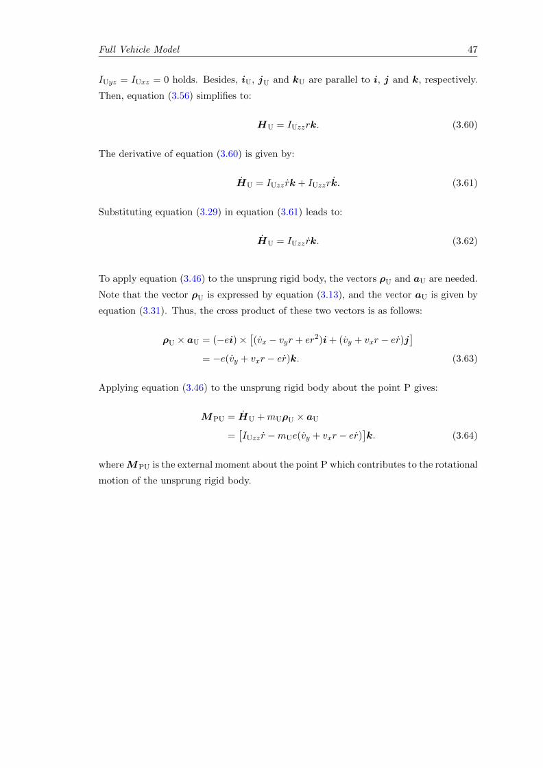
Full Vehicle Model 47
IUyz = IUxz = 0 holds. Besides, iU, jU and kU are parallel to i, j and k, respectively.
Then, equation (3.56) simplifies to:
HU = IUzzrk. (3.60)
The derivative of equation (3.60) is given by:
HU = IUzz rk + IUzzrk. (3.61)
Substituting equation (3.29) in equation (3.61) leads to:
HU = IUzz rk. (3.62)
To apply equation (3.46) to the unsprung rigid body, the vectors ρU and aU are needed.
Note that the vector ρU is expressed by equation (3.13), and the vector aU is given by
equation (3.31). Thus, the cross product of these two vectors is as follows:
ρU × aU = (−ei)×[(vx − vyr + er2)i+ (vy + vxr − er)j
]
= −e(vy + vxr − er)k. (3.63)
Applying equation (3.46) to the unsprung rigid body about the point P gives:
MPU = HU +mUρU × aU=[IUzz r −mUe(vy + vxr − er)
]k. (3.64)
whereMPU is the external moment about the point P which contributes to the rotational
motion of the unsprung rigid body.
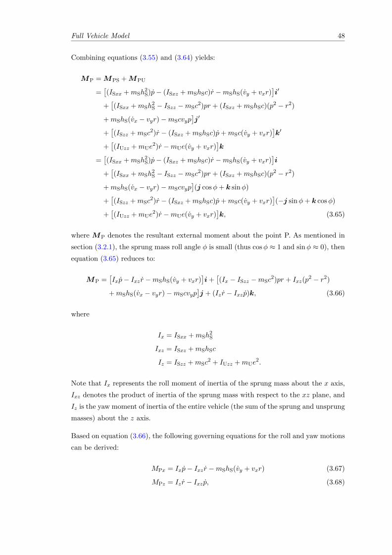
Full Vehicle Model 48
Combining equations (3.55) and (3.64) yields:
MP = MPS +MPU
=[(ISxx +mSh
2S)p− (ISxz +mShSc)r −mShS(vy + vxr)
]i′
+[(ISxx +mSh
2S − ISzz −mSc
2)pr + (ISxz +mShSc)(p2 − r2)
+mShS(vx − vyr)−mScvyp]j′
+[(ISzz +mSc
2)r − (ISxz +mShSc)p+mSc(vy + vxr)]k′
+[(IUzz +mUe
2)r −mUe(vy + vxr)]k
=[(ISxx +mSh
2S)p− (ISxz +mShSc)r −mShS(vy + vxr)
]i
+[(ISxx +mSh
2S − ISzz −mSc
2)pr + (ISxz +mShSc)(p2 − r2)
+mShS(vx − vyr)−mScvyp](j cosφ+ k sinφ)
+[(ISzz +mSc
2)r − (ISxz +mShSc)p+mSc(vy + vxr)](−j sinφ+ k cosφ)
+[(IUzz +mUe
2)r −mUe(vy + vxr)]k, (3.65)
where MP denotes the resultant external moment about the point P. As mentioned in
section (3.2.1), the sprung mass roll angle φ is small (thus cosφ ≈ 1 and sinφ ≈ 0), then
equation (3.65) reduces to:
MP =[Ixp− Ixz r −mShS(vy + vxr)
]i+
[(Ix − ISzz −mSc
2)pr + Ixz(p2 − r2)
+mShS(vx − vyr)−mScvyp]j + (Iz r − Ixz p)k, (3.66)
where
Ix = ISxx +mSh2S
Ixz = ISxz +mShSc
Iz = ISzz +mSc2 + IUzz +mUe
2.
Note that Ix represents the roll moment of inertia of the sprung mass about the x axis,
Ixz denotes the product of inertia of the sprung mass with respect to the xz plane, and
Iz is the yaw moment of inertia of the entire vehicle (the sum of the sprung and unsprung
masses) about the z axis.
Based on equation (3.66), the following governing equations for the roll and yaw motions
can be derived:
MPx = Ixp− Ixz r −mShS(vy + vxr) (3.67)
MPz = Iz r − Ixz p, (3.68)
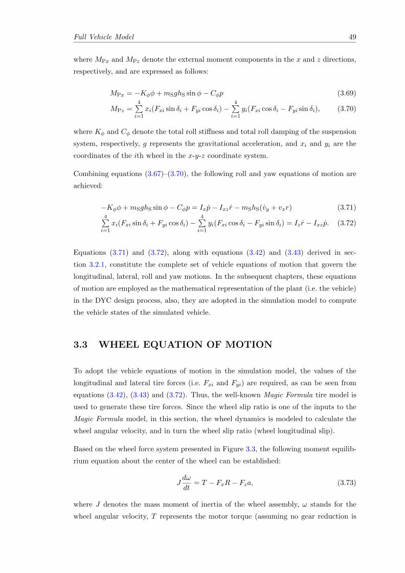
Full Vehicle Model 49
where MPx and MPz denote the external moment components in the x and z directions,
respectively, and are expressed as follows:
MPx = −Kφφ+mSghS sinφ− Cφp (3.69)
MPz =4∑i=1
xi(Fxi sin δi + Fyi cos δi)−4∑i=1
yi(Fxi cos δi − Fyi sin δi), (3.70)
where Kφ and Cφ denote the total roll stiffness and total roll damping of the suspension
system, respectively, g represents the gravitational acceleration, and xi and yi are the
coordinates of the ith wheel in the x-y-z coordinate system.
Combining equations (3.67)–(3.70), the following roll and yaw equations of motion are
achieved:
−Kφφ+mSghS sinφ− Cφp = Ixp− Ixz r −mShS(vy + vxr) (3.71)4∑i=1
xi(Fxi sin δi + Fyi cos δi)−4∑i=1
yi(Fxi cos δi − Fyi sin δi) = Iz r − Ixz p. (3.72)
Equations (3.71) and (3.72), along with equations (3.42) and (3.43) derived in sec-
tion 3.2.1, constitute the complete set of vehicle equations of motion that govern the
longitudinal, lateral, roll and yaw motions. In the subsequent chapters, these equations
of motion are employed as the mathematical representation of the plant (i.e. the vehicle)
in the DYC design process, also, they are adopted in the simulation model to compute
the vehicle states of the simulated vehicle.
3.3 WHEEL EQUATION OF MOTION
To adopt the vehicle equations of motion in the simulation model, the values of the
longitudinal and lateral tire forces (i.e. Fxi and Fyi) are required, as can be seen from
equations (3.42), (3.43) and (3.72). Thus, the well-known Magic Formula tire model is
used to generate these tire forces. Since the wheel slip ratio is one of the inputs to the
Magic Formula model, in this section, the wheel dynamics is modeled to calculate the
wheel angular velocity, and in turn the wheel slip ratio (wheel longitudinal slip).
Based on the wheel force system presented in Figure 3.3, the following moment equilib-
rium equation about the center of the wheel can be established:
Jdω
dt= T − FxR− Fza, (3.73)
where J denotes the mass moment of inertia of the wheel assembly, ω stands for the
wheel angular velocity, T represents the motor torque (assuming no gear reduction is
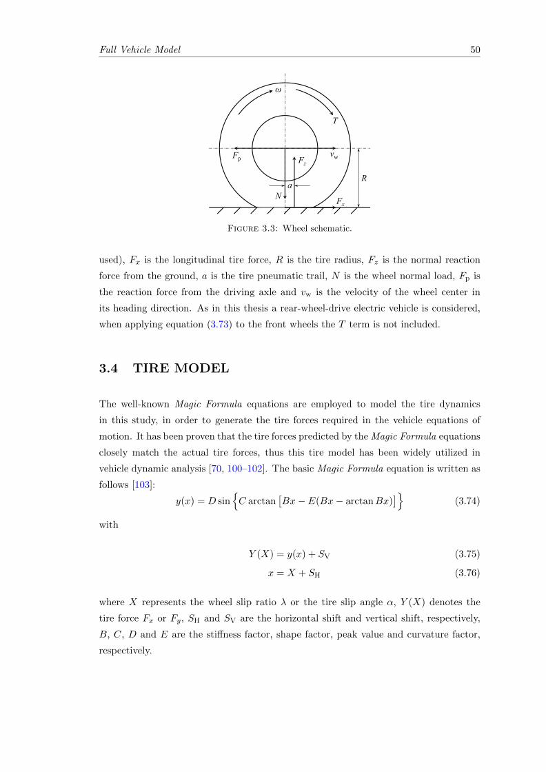
Full Vehicle Model 50
Fx
Fz
T
R
Na
ω
Fp vw
Figure 3.3: Wheel schematic.
used), Fx is the longitudinal tire force, R is the tire radius, Fz is the normal reaction
force from the ground, a is the tire pneumatic trail, N is the wheel normal load, Fp is
the reaction force from the driving axle and vw is the velocity of the wheel center in
its heading direction. As in this thesis a rear-wheel-drive electric vehicle is considered,
when applying equation (3.73) to the front wheels the T term is not included.
3.4 TIRE MODEL
The well-known Magic Formula equations are employed to model the tire dynamics
in this study, in order to generate the tire forces required in the vehicle equations of
motion. It has been proven that the tire forces predicted by the Magic Formula equations
closely match the actual tire forces, thus this tire model has been widely utilized in
vehicle dynamic analysis [70, 100–102]. The basic Magic Formula equation is written as
follows [103]:
y(x) = D sin{C arctan
[Bx− E(Bx− arctanBx)
]}(3.74)
with
Y (X) = y(x) + SV (3.75)
x = X + SH (3.76)
where X represents the wheel slip ratio λ or the tire slip angle α, Y (X) denotes the
tire force Fx or Fy, SH and SV are the horizontal shift and vertical shift, respectively,
B, C, D and E are the stiffness factor, shape factor, peak value and curvature factor,
respectively.
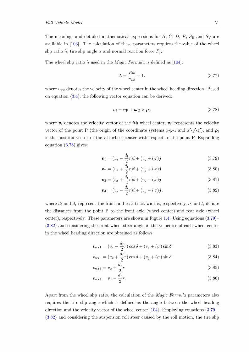
Full Vehicle Model 51
The meanings and detailed mathematical expressions for B, C, D, E, SH and SV are
available in [103]. The calculation of these parameters requires the value of the wheel
slip ratio λ, tire slip angle α and normal reaction force Fz.
The wheel slip ratio λ used in the Magic Formula is defined as [104]:
λ =Rω
vwx− 1. (3.77)
where vwx denotes the velocity of the wheel center in the wheel heading direction. Based
on equation (3.4), the following vector equation can be derived:
vi = vP + ωU × ρi, (3.78)
where vi denotes the velocity vector of the ith wheel center, vP represents the velocity
vector of the point P (the origin of the coordinate systems x-y-z and x′-y′-z′), and ρi
is the position vector of the ith wheel center with respect to the point P. Expanding
equation (3.78) gives:
v1 = (vx −df2r)i+ (vy + lfr)j (3.79)
v2 = (vx +df2r)i+ (vy + lfr)j (3.80)
v3 = (vx +dr2r)i+ (vy − lrr)j (3.81)
v4 = (vx −dr2r)i+ (vy − lrr)j, (3.82)
where df and dr represent the front and rear track widths, respectively, lf and lr denote
the distances from the point P to the front axle (wheel center) and rear axle (wheel
center), respectively. These parameters are shown in Figure 1.4. Using equations (3.79)–
(3.82) and considering the front wheel steer angle δ, the velocities of each wheel center
in the wheel heading direction are obtained as follows:
vwx1 = (vx −df2r) cos δ + (vy + lfr) sin δ (3.83)
vwx2 = (vx +df2r) cos δ + (vy + lfr) sin δ (3.84)
vwx3 = vx +dr2r (3.85)
vwx4 = vx −dr2r. (3.86)
Apart from the wheel slip ratio, the calculation of the Magic Formula parameters also
requires the tire slip angle which is defined as the angle between the wheel heading
direction and the velocity vector of the wheel center [104]. Employing equations (3.79)–
(3.82) and considering the suspension roll steer caused by the roll motion, the tire slip
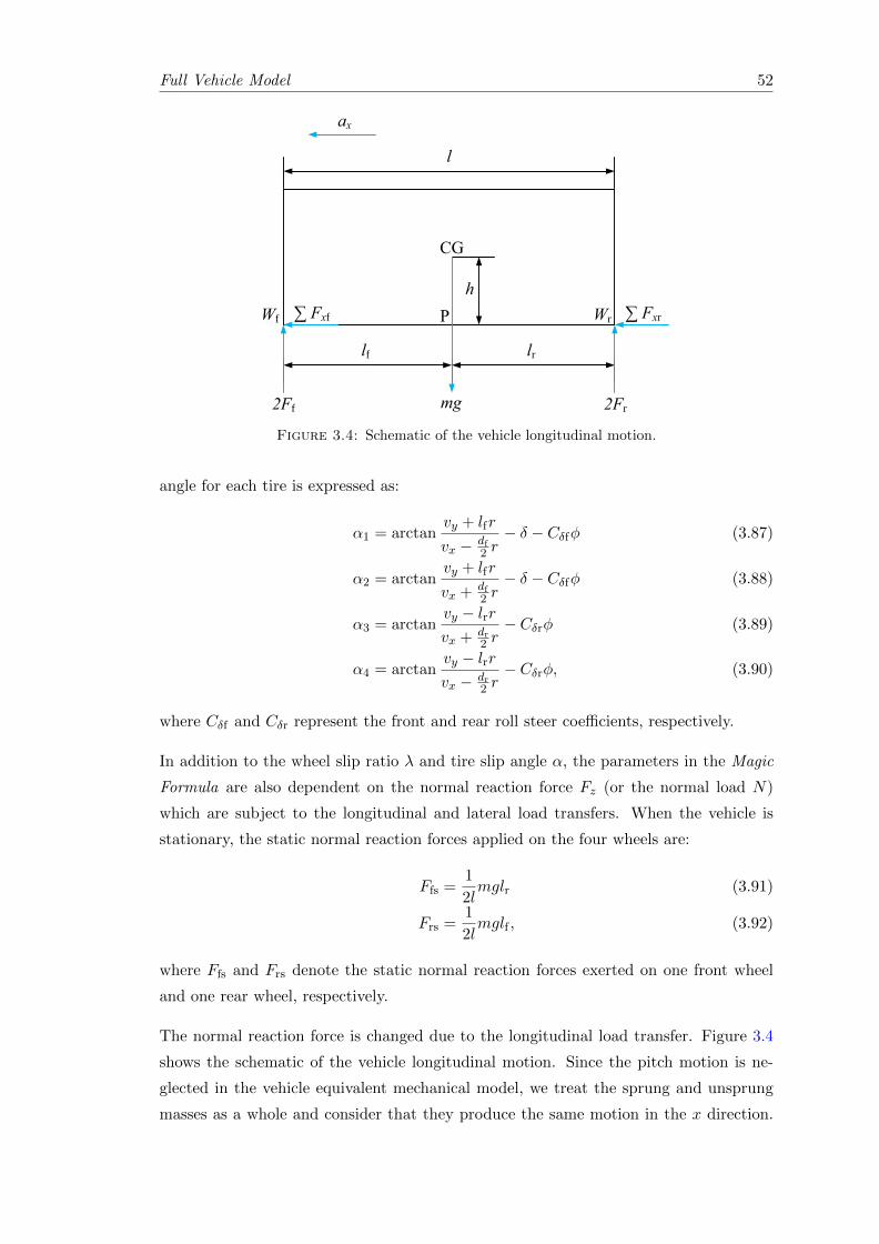
Full Vehicle Model 52
l
lrlf
h
mg2Ff 2Fr
ax
Wf Wr∑ Fxf ∑ Fxr
Figure 3.4: Schematic of the vehicle longitudinal motion.
angle for each tire is expressed as:
α1 = arctanvy + lfr
vx − df2 r− δ − Cδfφ (3.87)
α2 = arctanvy + lfr
vx + df2 r− δ − Cδfφ (3.88)
α3 = arctanvy − lrrvx + dr
2 r− Cδrφ (3.89)
α4 = arctanvy − lrrvx − dr
2 r− Cδrφ, (3.90)
where Cδf and Cδr represent the front and rear roll steer coefficients, respectively.
In addition to the wheel slip ratio λ and tire slip angle α, the parameters in the Magic
Formula are also dependent on the normal reaction force Fz (or the normal load N)
which are subject to the longitudinal and lateral load transfers. When the vehicle is
stationary, the static normal reaction forces applied on the four wheels are:
Ffs =1
2lmglr (3.91)
Frs =1
2lmglf , (3.92)
where Ffs and Frs denote the static normal reaction forces exerted on one front wheel
and one rear wheel, respectively.
The normal reaction force is changed due to the longitudinal load transfer. Figure 3.4
shows the schematic of the vehicle longitudinal motion. Since the pitch motion is ne-
glected in the vehicle equivalent mechanical model, we treat the sprung and unsprung
masses as a whole and consider that they produce the same motion in the x direction.
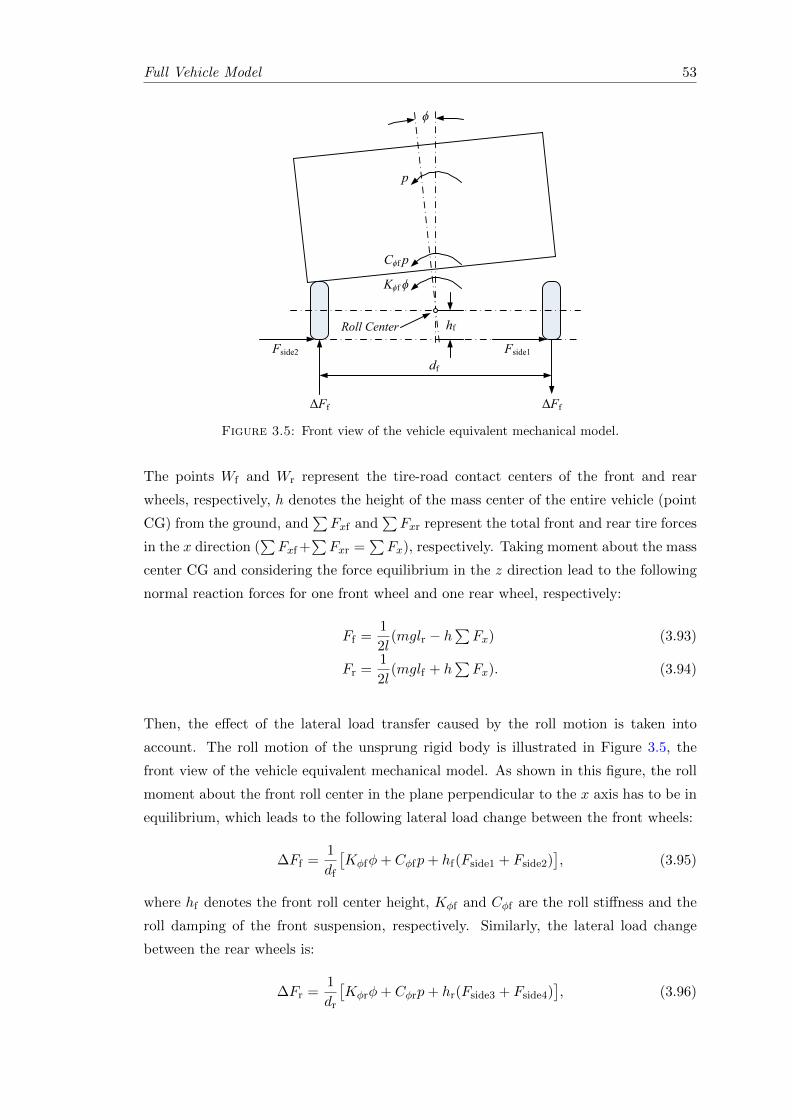
Full Vehicle Model 53
df
hf
ϕ
Kϕf ϕ
Cϕf p
Roll Center
Fside1Fside2
p
ΔFfΔFf
Figure 3.5: Front view of the vehicle equivalent mechanical model.
The points Wf and Wr represent the tire-road contact centers of the front and rear
wheels, respectively, h denotes the height of the mass center of the entire vehicle (point
CG) from the ground, and∑Fxf and
∑Fxr represent the total front and rear tire forces
in the x direction (∑Fxf +
∑Fxr =
∑Fx), respectively. Taking moment about the mass
center CG and considering the force equilibrium in the z direction lead to the following
normal reaction forces for one front wheel and one rear wheel, respectively:
Ff =1
2l(mglr − h
∑Fx) (3.93)
Fr =1
2l(mglf + h
∑Fx). (3.94)
Then, the effect of the lateral load transfer caused by the roll motion is taken into
account. The roll motion of the unsprung rigid body is illustrated in Figure 3.5, the
front view of the vehicle equivalent mechanical model. As shown in this figure, the roll
moment about the front roll center in the plane perpendicular to the x axis has to be in
equilibrium, which leads to the following lateral load change between the front wheels:
∆Ff =1
df
[Kφfφ+ Cφfp+ hf(Fside1 + Fside2)
], (3.95)
where hf denotes the front roll center height, Kφf and Cφf are the roll stiffness and the
roll damping of the front suspension, respectively. Similarly, the lateral load change
between the rear wheels is:
∆Fr =1
dr
[Kφrφ+ Cφrp+ hr(Fside3 + Fside4)
], (3.96)
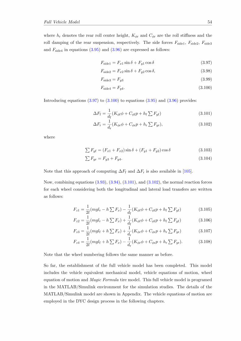
Full Vehicle Model 54
where hr denotes the rear roll center height, Kφr and Cφr are the roll stiffness and the
roll damping of the rear suspension, respectively. The side forces Fside1, Fside2, Fside3
and Fside4 in equations (3.95) and (3.96) are expressed as follows:
Fside1 = Fx1 sin δ + Fy1 cos δ (3.97)
Fside2 = Fx2 sin δ + Fy2 cos δ, (3.98)
Fside3 = Fy3 (3.99)
Fside4 = Fy4. (3.100)
Introducing equations (3.97) to (3.100) to equations (3.95) and (3.96) provides:
∆Ff =1
df(Kφfφ+ Cφfp+ hf
∑Fyf) (3.101)
∆Fr =1
dr(Kφrφ+ Cφrp+ hr
∑Fyr), (3.102)
where
∑Fyf = (Fx1 + Fx2) sin δ + (Fy1 + Fy2) cos δ (3.103)
∑Fyr = Fy3 + Fy4. (3.104)
Note that this approach of computing ∆Ff and ∆Fr is also available in [105].
Now, combining equations (3.93), (3.94), (3.101), and (3.102), the normal reaction forces
for each wheel considering both the longitudinal and lateral load transfers are written
as follows:
Fz1 =1
2l(mglr − h
∑Fx)− 1
df(Kφfφ+ Cφfp+ hf
∑Fyf) (3.105)
Fz2 =1
2l(mglr − h
∑Fx) +
1
df(Kφfφ+ Cφfp+ hf
∑Fyf) (3.106)
Fz3 =1
2l(mglf + h
∑Fx) +
1
dr(Kφrφ+ Cφrp+ hr
∑Fyr) (3.107)
Fz4 =1
2l(mglf + h
∑Fx)− 1
dr(Kφrφ+ Cφrp+ hr
∑Fyr). (3.108)
Note that the wheel numbering follows the same manner as before.
So far, the establishment of the full vehicle model has been completed. This model
includes the vehicle equivalent mechanical model, vehicle equations of motion, wheel
equation of motion and Magic Formula tire model. This full vehicle model is programed
in the MATLAB/Simulink environment for the simulation studies. The details of the
MATLAB/Simulink model are shown in Appendix. The vehicle equations of motion are
employed in the DYC design process in the following chapters.
Chapter 4
Yaw Rate-Based Direct Yaw
Moment Control
In this chapter, a mathematical relationship between the yaw rate and the corrective yaw
moment produced by the DYC system is derived from the vehicle equations of motion
established in Chapter 3. This mathematical relationship reveals that the steady-state
yaw rate directly depends on the torque difference between the left and right driving
motors, which implies that it can be controlled by tuning this torque difference. Based
on this relationship, a yaw rate-based DYC method is proposed to achieve neutral steer.
Comparative simulation results show that the proposed DYC method closely tracks
the reference yaw rate associated with neutral steer, also it outperforms the competing
methods in terms of tracking the desired yaw rate and vehicle path in various driving
scenarios.
4.1 BACKGROUND
As introduced in Chapter 1, the yaw rate r is the vehicle angular velocity about the z
axis of the vehicle local coordinate x-y-z, as shown in Figure 1.4. The yaw rate plays
a crucial roll in vehicle stability and handling control, and is one of the main control
variables for DYC systems. Firstly, the steady-state yaw rate (derived from the common
bicycle model) is a function of the front wheel steer angle. So, it is interpreted as the
vehicle response commanded by the driver. Secondly, this steady-state yaw rate value
defines the steer characteristic (i.e. under, over, or neutral steer) of the vehicle. To
enhance vehicle handling, in this chapter a yaw rate-based DYC method is proposed to
drive the yaw rate towards a desired/target value that would lead to neutral steer.
55
Yaw Rate-Based Direct Yaw Moment Control 56
In Chapter 2, several typical types of control methods have been reviewed, including the
equal torque methods [27–33], the Ackerman methods [38–46] and the yaw rate-based
DYC methods which employ equation (2.5) with a positive K as the reference yaw
rate [48, 50, 54, 55]. In the simulation studies in this chapter, to verify the effectiveness
of the proposed DYC, the control performances of the proposed method and the aforesaid
three types of methods are compared. Here, the concepts and principles behind these
methods are recalled.
The equal torque methods are the most straightforward solutions for controlling two
independent motors. They emulate the behavior of an open differential by applying
equal torques to the two driving wheels. Thus, these methods provide the electric
vehicle with a cornering performance similar to an ICE vehicle equipped with an open
differential. Actually, the equal torque methods cannot be categorized as DYC systems,
as no active yaw moment can be generated to regulate vehicle motion.
The Ackerman methods use the vehicle speed and the front wheel steer angle the as input
parameters and calculate the required inner and outer wheel angular velocities, by means
of the well-known Ackerman steering geometry. When the electric vehicle enters a corner,
the control system acts immediately on both motors, reducing the angular velocity of the
inner wheel while increasing that of the outer wheel [38] to their desired values defined
by equations (2.2) and (2.3). In the simulation studies, to examine the performance
of the Ackerman methods, the driving wheel angular velocities have been tuned based
on their sum and difference, with the sum being proportional to the speed command
read from the throttle pedal sensor and the difference computed from equations (2.2)
and (2.3) as follows:
∆ω = ωR − ωL =vrdr tan δ
Rl. (4.1)
Note that neither the equal torque methods nor the Ackerman methods take into account
the vehicle dynamics. New DYC designs have been proposed in the literature to incor-
porate the vehicle dynamics, by maintaining the yaw rate at a desired level determined
by a planar vehicle dynamic model. This desired yaw rate is described by equation (2.5)
in which the stability factor K is normally maintained at a positive value to provide
sufficient stability margin for the vehicle. However, a positive stability factor causes
understeer and makes the vehicle “reluctant” to turn, which is not optimum for vehicle
handling. In the proposed DYC design, K = 0 is selected to achieve the ideal steer
characteristic, neutral steer, without impairing the vehicle stability. The advantageous
vehicle handling performance with no loss in the stability is fully demonstrated in highly
challenging driving scenarios, as presented in the simulation results.
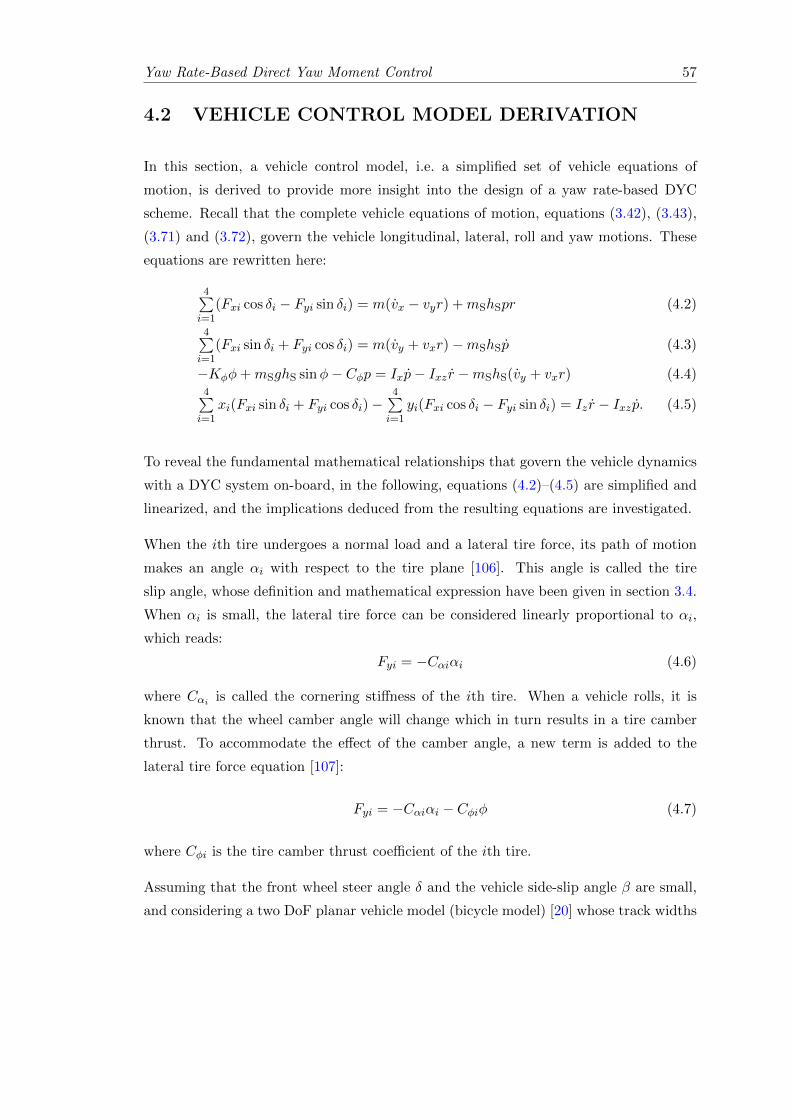
Yaw Rate-Based Direct Yaw Moment Control 57
4.2 VEHICLE CONTROL MODEL DERIVATION
In this section, a vehicle control model, i.e. a simplified set of vehicle equations of
motion, is derived to provide more insight into the design of a yaw rate-based DYC
scheme. Recall that the complete vehicle equations of motion, equations (3.42), (3.43),
(3.71) and (3.72), govern the vehicle longitudinal, lateral, roll and yaw motions. These
equations are rewritten here:
4∑i=1
(Fxi cos δi − Fyi sin δi) = m(vx − vyr) +mShSpr (4.2)
4∑i=1
(Fxi sin δi + Fyi cos δi) = m(vy + vxr)−mShSp (4.3)
−Kφφ+mSghS sinφ− Cφp = Ixp− Ixz r −mShS(vy + vxr) (4.4)4∑i=1
xi(Fxi sin δi + Fyi cos δi)−4∑i=1
yi(Fxi cos δi − Fyi sin δi) = Iz r − Ixz p. (4.5)
To reveal the fundamental mathematical relationships that govern the vehicle dynamics
with a DYC system on-board, in the following, equations (4.2)–(4.5) are simplified and
linearized, and the implications deduced from the resulting equations are investigated.
When the ith tire undergoes a normal load and a lateral tire force, its path of motion
makes an angle αi with respect to the tire plane [106]. This angle is called the tire
slip angle, whose definition and mathematical expression have been given in section 3.4.
When αi is small, the lateral tire force can be considered linearly proportional to αi,
which reads:
Fyi = −Cαiαi (4.6)
where Cαi is called the cornering stiffness of the ith tire. When a vehicle rolls, it is
known that the wheel camber angle will change which in turn results in a tire camber
thrust. To accommodate the effect of the camber angle, a new term is added to the
lateral tire force equation [107]:
Fyi = −Cαiαi − Cφiφ (4.7)
where Cφi is the tire camber thrust coefficient of the ith tire.
Assuming that the front wheel steer angle δ and the vehicle side-slip angle β are small,
and considering a two DoF planar vehicle model (bicycle model) [20] whose track widths

Yaw Rate-Based Direct Yaw Moment Control 58
are neglected, the mathematical expressions of the tire slip angles (equations (3.87)–
(3.90)) can be simplified to
α1 = α2 ≈vy + lfr
vx− δ − Cδfφ ≈ β +
lfr
vx− δ − Cδfφ (4.8)
α3 = α4 ≈vy − lrrvx
− Cδrφ ≈ β −lrr
vx− Cδrφ. (4.9)
Substituting equations (4.8) and (4.9) in equation (4.7), the following lateral tire force
expressions for the four wheels are obtained:
Fy1 = −Cα1(β +lfr
vx− δ − Cδfφ)− Cφ1φ (4.10)
Fy2 = −Cα2(β +lfr
vx− δ − Cδfφ)− Cφ2φ (4.11)
Fy3 = −Cα3(β −lrr
vx− Cδrφ)− Cφ3φ (4.12)
Fy4 = −Cα4(β −lrr
vx− Cδrφ)− Cφ4φ. (4.13)
It is assumed that the longitudinal tire forces are symmetric, i.e. Fx1 = Fx2 and Fx3 =
Fx4, and that the front wheel steer angle δ and the sprung mass roll angle φ are both
small (thus sin δ ≈ 0, cos δ ≈ 1 and sinφ ≈ φ). Then, substituting equations (4.10)–
(4.13) in the left-hand side terms in equations (4.2)–(4.5) leads to:
∑Fx = Fx1 + Fx2 + Fx3 + Fx4 (4.14)
∑Fy = −Cαf(β +
lfr
vx− δ − Cδfφ)− Cφfφ− Cαr(β −
lrr
vx− Cδrφ)− Cφrφ (4.15)
MPx = −Kφφ+mSghSφ− Cφp (4.16)
MPz = −lf[Cαf(β +
lfr
vx− δ − Cδfφ) + Cφfφ
]+ lr
[Cαr(β −
lrr
vx− Cδrφ) + Cφrφ
](4.17)
where Cαf = Cα1 + Cα2 and Cαr = Cα3 + Cα4 are the sums of the left and right tire
cornering stiffnesses for the front tires and rear tires, respectively, and Cφf = Cφ1 +Cφ2
and Cφr = Cφ3 + Cφ4 are the sums of the left and right tire camber thrust coefficients
for the front tires and rear tires, respectively.
To retain the linearity of the equations of motion, in the following analysis, the vehicle
longitudinal dynamics is neglected (assuming vx is constant). Note that the vehicle
longitudinal motion is generated due to traction and braking without direct relation
to steering, thus this motion is not directly connected to the vehicle lateral and yaw
motions which are generated by steering the vehicle [96]. Hence, it is a common practice
to neglect the vehicle longitudinal dynamics when the focus is on the vehicle lateral and
yaw behaviors [108, 109].
Yaw Rate-Based Direct Yaw Moment Control 59
Equation (4.14) is no more considered as the vehicle longitudinal dynamics is neglected,
then equations (4.15)–(4.17) are rearranged as follows:
∑Fy = aββ + arr + aφφ+ aδδ (4.18)
MPx = bφφ+ bpp (4.19)
MPz = cββ + crr + cφφ+ cδδ, (4.20)
where,
aβ = −Cαf − Cαr (4.21)
ar = −Cαflfvx
+ Cαrlrvx
(4.22)
aφ = CαfCδf − Cφf + CαrCδr − Cφr (4.23)
aδ = Cαf (4.24)
bφ = −Kφ +mSghS (4.25)
bp = −Cφ (4.26)
cβ = −lfCαf + lrCαr (4.27)
cr = −Cαfl2fvx− Cαr
l2rvx
(4.28)
cφ = lfCαfCδf − lfCφf − lrCαrCδr + lrCφr (4.29)
cδ = lfCαf . (4.30)
Thus, equations (4.3)–(4.5) which govern the vehicle lateral, roll and yaw motions can
be rewritten as:
aββ + arr + aφφ+ aδδ = m(vy + vxr)−mShSp (4.31)
bφφ+ bpp = Ixp− Ixz r −mShS(vy + vxr) (4.32)
cββ + crr + cφφ+ cδδ = Iz r − Ixz p. (4.33)
The simplified vehicle equations of motion (4.31)–(4.33) constitute the vehicle control
model, and they will be adopted in the next section to derive the control law for the
proposed yaw rate-based DYC system.
So far, the small angle assumption has been employed several times in the above deriva-
tions. It is important to justify that the usage of the small angle assumption retains the
validity of the above simplified vehicle equations of motion (4.31)–(4.33).
The application of the small angle assumption to α can be justified by an example
in [110], a typical racing tire inflated at 31 psi for a given load of 1800 lb. This Goodyear
racing tire provides the maximum lateral force at a tire slip angle of about 6.5◦ after
Yaw Rate-Based Direct Yaw Moment Control 60
which the tire enters an unstable frictional range. Notice that 6.5◦ is only about 0.1 rad
and the tire normally operates in the range below 6.5◦, which allows a safe application
of the small angle assumption to α in the linearization.
As for δ, assuming a steering ratio of 1:12, a small front wheel steer angle of 0.2 rad
is corresponding to a steering wheel/column angle of about 138◦. At a medium vehicle
speed, say 60 km/h, this steer angle is a typical marginal magnitude beyond which the
vehicle tends to lose stability. So in the stable region, the vehicle will mostly operate
with a smaller steer angle at that speed, which in turn makes it justified to apply the
small angle assumption to the front wheel steer angle δ.
Furthermore, when both α and δ are assumed to be small, the associated vehicle side-slip
angle β becomes small as well. Summing up the above points, the vehicle control model
(i.e. the simplified vehicle equations of motion (4.31)–(4.33)) obtained by means of small
angle assumptions are practically valid and can capture the major characteristics of the
vehicle dynamics. As can be seen in the next section, this model is utilized to derive the
relationship between the steady-state yaw rate and the left-right motor torque difference,
based on which the proposed DYC system is designed.
4.3 YAW RATE-BASED DYC DESIGN
The proposed design, as a direct yaw moment control system, is based on independently
generating different torque commands to the two driving motors. Different motor torques
are intuitively expected to generate different longitudinal tire forces on the driving wheels
to produce a yaw moment. In this section, using the vehicle control model obtained in
section 4.2, an equation showing a direct relationship between the steady-state yaw rate
and the torque difference between the left and right driving motors is derived. Based
on this mathematical relationship, a yaw rate-based DYC system is proposed to achieve
the ideal steer characteristic, neutral steer.
With a DYC system on-board, there can be a difference between the longitudinal tire
forces of the two rear driving wheels. Denoting this difference by ∆Fx = Fx3−Fx4, it can
be seen that the effect of ∆Fx is equivalent to an additional moment ∆M = ∆Fx × d/2applied on the rear axle plus a force ∆Fx exerted at the center of the rear axle, as
illustrated in Figure 4.1. Thus, in presence of the difference between the tire forces, only
equation (4.33) needs to be modified as follows:
cββ + crr + cφφ+ cδδ +dr2·∆Fx = Iz r − Ixz p. (4.34)
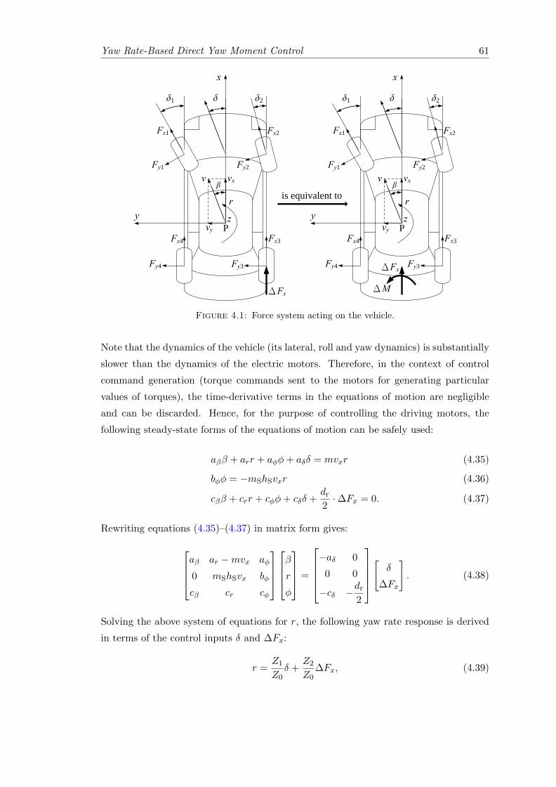
Yaw Rate-Based Direct Yaw Moment Control 61
Fy1
Fx1 Fx2
Fy2
Fx4
Fy4 Fy3
Fx3
x
yP
δ2δ1
vx
vy
r
δ
z
βv
Fy1
Fx1 Fx2
Fy2
Fx4
Fy4 Fy3
Fx3
x
yP
δ2δ1
vx
vy
r
δ
z
βv
is equivalent to
ΔFx
ΔFx
ΔM
Figure 4.1: Force system acting on the vehicle.
Note that the dynamics of the vehicle (its lateral, roll and yaw dynamics) is substantially
slower than the dynamics of the electric motors. Therefore, in the context of control
command generation (torque commands sent to the motors for generating particular
values of torques), the time-derivative terms in the equations of motion are negligible
and can be discarded. Hence, for the purpose of controlling the driving motors, the
following steady-state forms of the equations of motion can be safely used:
aββ + arr + aφφ+ aδδ = mvxr (4.35)
bφφ = −mShSvxr (4.36)
cββ + crr + cφφ+ cδδ +dr2·∆Fx = 0. (4.37)
Rewriting equations (4.35)–(4.37) in matrix form gives:
aβ ar −mvx aφ
0 mShSvx bφ
cβ cr cφ
β
r
φ
=
−aδ 0
0 0
−cδ −dr2
[δ
∆Fx
]. (4.38)
Solving the above system of equations for r, the following yaw rate response is derived
in terms of the control inputs δ and ∆Fx:
r =Z1
Z0δ +
Z2
Z0∆Fx, (4.39)
Yaw Rate-Based Direct Yaw Moment Control 62
where,
Z0 = aβbφcr − arbφcβ + bφcβmvx − aβcφmShSvx + aφcβmShSvx (4.40)
Z1 = bφ(aδcβ − aβcδ) (4.41)
Z2 = −1
2aβbφdr. (4.42)
Equation (4.39) shows a direct relationship between the steady-state yaw rate and the
longitudinal tire force difference ∆Fx.
As mentioned earlier, compared to the dynamics of the electric motors, the dynamics of
the mechanical parts is very slow. Particularly, during each sampling time of the elec-
tronic control system, the variation of the wheel angular velocity is negligible. Besides,
the tire pneumatic trail is normally quite small. Thus, neglecting the wheel angular
acceleration and the tire pneumatic trail simplifies equation (3.73) to:
T = FxR. (4.43)
This shows that the longitudinal tire forces (and their difference) can be directly con-
trolled by tuning the torque commands sent to the driving motors.
Substituting equation (4.43) in equation (4.39) leads to:
r =Z1
Z0δ +
Z2
Z0R∆T. (4.44)
Equation (4.44) clearly demonstrates a direct relationship between the steady-state yaw
rate and the difference between the two motor torques, ∆T . This implies that by
controlling the two motor torques, the vehicle steady-state yaw rate can be tuned to
attain its desired value.
To calculate the desired yaw rate, the main criterion for neutral steer behavior is con-
sidered: the vehicle’s instantaneous turning radius should not change with speed, as
introduced in section 2.3. Kinematically, the turning radius is known as L = v/r, where
v is the vehicle velocity at point P, as shown in Figure 1.4. Because the lateral com-
ponent of v is considerably smaller than its longitudinal component vx, so the tuning
radius can be approximated by L = vx/r.
Replacing vx with rL in the numerator of the fraction in equation (2.5), and solving for
L lead to:
L =l(1 +Kvx
2)
δ. (4.45)
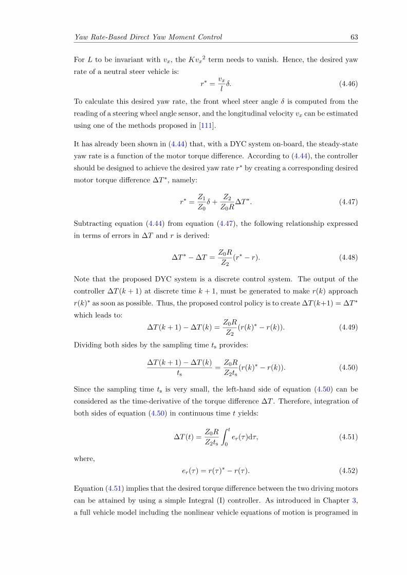
Yaw Rate-Based Direct Yaw Moment Control 63
For L to be invariant with vx, the Kvx2 term needs to vanish. Hence, the desired yaw
rate of a neutral steer vehicle is:
r∗ =vxlδ. (4.46)
To calculate this desired yaw rate, the front wheel steer angle δ is computed from the
reading of a steering wheel angle sensor, and the longitudinal velocity vx can be estimated
using one of the methods proposed in [111].
It has already been shown in (4.44) that, with a DYC system on-board, the steady-state
yaw rate is a function of the motor torque difference. According to (4.44), the controller
should be designed to achieve the desired yaw rate r∗ by creating a corresponding desired
motor torque difference ∆T ∗, namely:
r∗ =Z1
Z0δ +
Z2
Z0R∆T ∗. (4.47)
Subtracting equation (4.44) from equation (4.47), the following relationship expressed
in terms of errors in ∆T and r is derived:
∆T ∗ −∆T =Z0R
Z2(r∗ − r). (4.48)
Note that the proposed DYC system is a discrete control system. The output of the
controller ∆T (k + 1) at discrete time k + 1, must be generated to make r(k) approach
r(k)∗ as soon as possible. Thus, the proposed control policy is to create ∆T (k+1) = ∆T ∗
which leads to:
∆T (k + 1)−∆T (k) =Z0R
Z2(r(k)∗ − r(k)). (4.49)
Dividing both sides by the sampling time ts provides:
∆T (k + 1)−∆T (k)
ts=Z0R
Z2ts(r(k)∗ − r(k)). (4.50)
Since the sampling time ts is very small, the left-hand side of equation (4.50) can be
considered as the time-derivative of the torque difference ∆T . Therefore, integration of
both sides of equation (4.50) in continuous time t yields:
∆T (t) =Z0R
Z2ts
∫ t
0er(τ)dτ, (4.51)
where,
er(τ) = r(τ)∗ − r(τ). (4.52)
Equation (4.51) implies that the desired torque difference between the two driving motors
can be attained by using a simple Integral (I) controller. As introduced in Chapter 3,
a full vehicle model including the nonlinear vehicle equations of motion is programed in
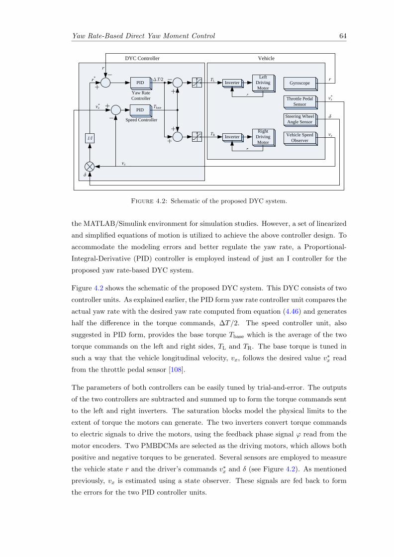
Yaw Rate-Based Direct Yaw Moment Control 64
PID
PIDLeft
Driving Motor
Gyroscope
Throttle Pedal Sensor
Inverter
Right Driving Motor
Inverter
Yaw Rate Controller
Speed Controller
ΔT/2
Tbase
TL
TR
Steering Wheel Angle Sensor
Vehicle Speed Observer1/l
r
δ
vx
δ
r*
r
DYC Controller Vehicle
vx
vx*
vx*
Figure 4.2: Schematic of the proposed DYC system.
the MATLAB/Simulink environment for simulation studies. However, a set of linearized
and simplified equations of motion is utilized to achieve the above controller design. To
accommodate the modeling errors and better regulate the yaw rate, a Proportional-
Integral-Derivative (PID) controller is employed instead of just an I controller for the
proposed yaw rate-based DYC system.
Figure 4.2 shows the schematic of the proposed DYC system. This DYC consists of two
controller units. As explained earlier, the PID form yaw rate controller unit compares the
actual yaw rate with the desired yaw rate computed from equation (4.46) and generates
half the difference in the torque commands, ∆T/2. The speed controller unit, also
suggested in PID form, provides the base torque Tbase which is the average of the two
torque commands on the left and right sides, TL and TR. The base torque is tuned in
such a way that the vehicle longitudinal velocity, vx, follows the desired value v∗x read
from the throttle pedal sensor [108].
The parameters of both controllers can be easily tuned by trial-and-error. The outputs
of the two controllers are subtracted and summed up to form the torque commands sent
to the left and right inverters. The saturation blocks model the physical limits to the
extent of torque the motors can generate. The two inverters convert torque commands
to electric signals to drive the motors, using the feedback phase signal ϕ read from the
motor encoders. Two PMBDCMs are selected as the driving motors, which allows both
positive and negative torques to be generated. Several sensors are employed to measure
the vehicle state r and the driver’s commands v∗x and δ (see Figure 4.2). As mentioned
previously, vx is estimated using a state observer. These signals are fed back to form
the errors for the two PID controller units.
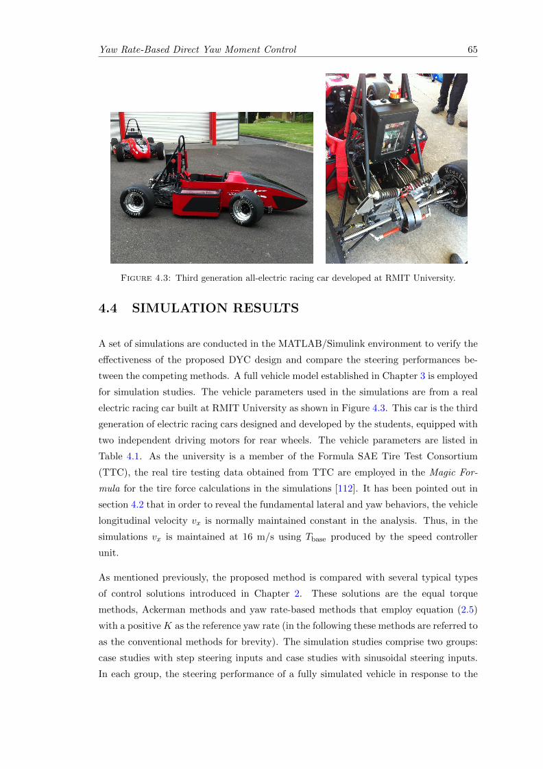
Yaw Rate-Based Direct Yaw Moment Control 65
Figure 4.3: Third generation all-electric racing car developed at RMIT University.
4.4 SIMULATION RESULTS
A set of simulations are conducted in the MATLAB/Simulink environment to verify the
effectiveness of the proposed DYC design and compare the steering performances be-
tween the competing methods. A full vehicle model established in Chapter 3 is employed
for simulation studies. The vehicle parameters used in the simulations are from a real
electric racing car built at RMIT University as shown in Figure 4.3. This car is the third
generation of electric racing cars designed and developed by the students, equipped with
two independent driving motors for rear wheels. The vehicle parameters are listed in
Table 4.1. As the university is a member of the Formula SAE Tire Test Consortium
(TTC), the real tire testing data obtained from TTC are employed in the Magic For-
mula for the tire force calculations in the simulations [112]. It has been pointed out in
section 4.2 that in order to reveal the fundamental lateral and yaw behaviors, the vehicle
longitudinal velocity vx is normally maintained constant in the analysis. Thus, in the
simulations vx is maintained at 16 m/s using Tbase produced by the speed controller
unit.
As mentioned previously, the proposed method is compared with several typical types
of control solutions introduced in Chapter 2. These solutions are the equal torque
methods, Ackerman methods and yaw rate-based methods that employ equation (2.5)
with a positive K as the reference yaw rate (in the following these methods are referred to
as the conventional methods for brevity). The simulation studies comprise two groups:
case studies with step steering inputs and case studies with sinusoidal steering inputs.
In each group, the steering performance of a fully simulated vehicle in response to the
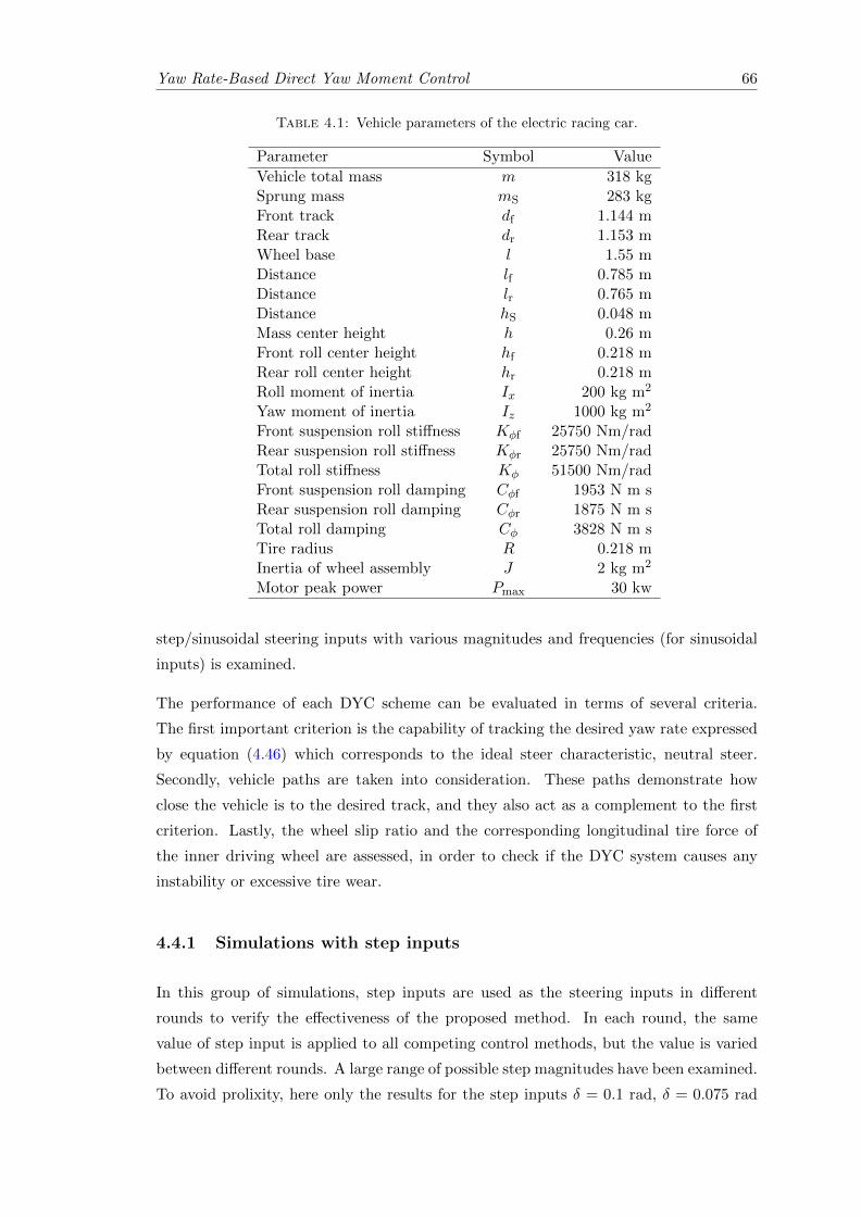
Yaw Rate-Based Direct Yaw Moment Control 66
Table 4.1: Vehicle parameters of the electric racing car.
Parameter Symbol Value
Vehicle total mass m 318 kgSprung mass mS 283 kgFront track df 1.144 mRear track dr 1.153 mWheel base l 1.55 mDistance lf 0.785 mDistance lr 0.765 mDistance hS 0.048 mMass center height h 0.26 mFront roll center height hf 0.218 mRear roll center height hr 0.218 mRoll moment of inertia Ix 200 kg m2
Yaw moment of inertia Iz 1000 kg m2
Front suspension roll stiffness Kφf 25750 Nm/radRear suspension roll stiffness Kφr 25750 Nm/radTotal roll stiffness Kφ 51500 Nm/radFront suspension roll damping Cφf 1953 N m sRear suspension roll damping Cφr 1875 N m sTotal roll damping Cφ 3828 N m sTire radius R 0.218 mInertia of wheel assembly J 2 kg m2
Motor peak power Pmax 30 kw
step/sinusoidal steering inputs with various magnitudes and frequencies (for sinusoidal
inputs) is examined.
The performance of each DYC scheme can be evaluated in terms of several criteria.
The first important criterion is the capability of tracking the desired yaw rate expressed
by equation (4.46) which corresponds to the ideal steer characteristic, neutral steer.
Secondly, vehicle paths are taken into consideration. These paths demonstrate how
close the vehicle is to the desired track, and they also act as a complement to the first
criterion. Lastly, the wheel slip ratio and the corresponding longitudinal tire force of
the inner driving wheel are assessed, in order to check if the DYC system causes any
instability or excessive tire wear.
4.4.1 Simulations with step inputs
In this group of simulations, step inputs are used as the steering inputs in different
rounds to verify the effectiveness of the proposed method. In each round, the same
value of step input is applied to all competing control methods, but the value is varied
between different rounds. A large range of possible step magnitudes have been examined.
To avoid prolixity, here only the results for the step inputs δ = 0.1 rad, δ = 0.075 rad
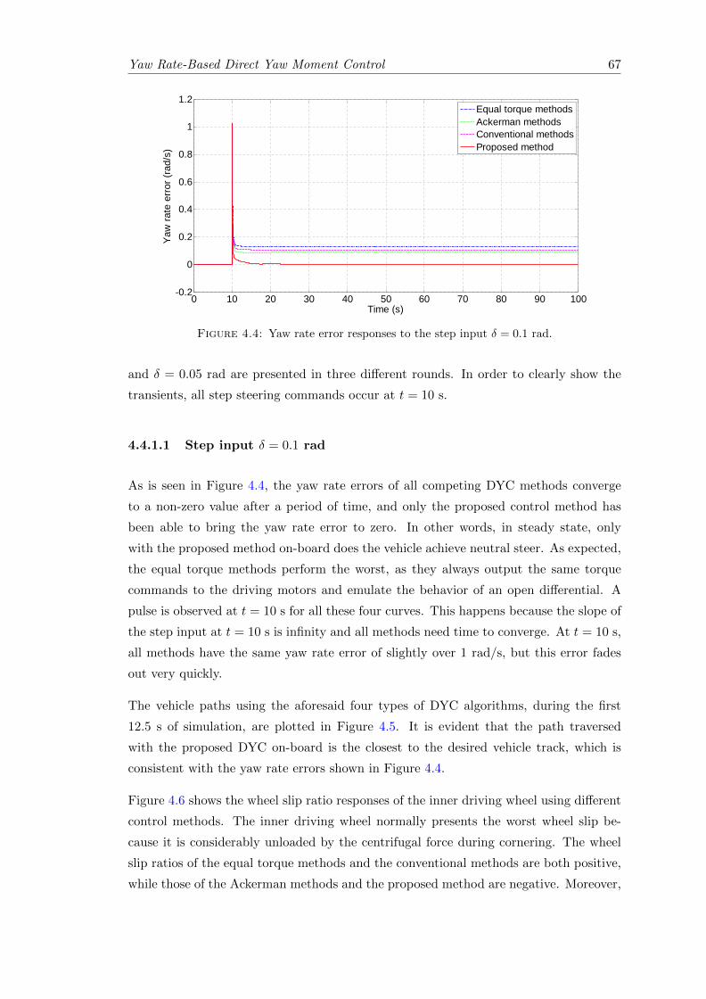
Yaw Rate-Based Direct Yaw Moment Control 67
0 10 20 30 40 50 60 70 80 90 100-0.2
0
0.2
0.4
0.6
0.8
1
1.2
Time (s)
Yaw
rate
erro
r (ra
d/s)
Equal torque methodsAckerman methodsConventional methodsProposed method
Figure 4.4: Yaw rate error responses to the step input δ = 0.1 rad.
and δ = 0.05 rad are presented in three different rounds. In order to clearly show the
transients, all step steering commands occur at t = 10 s.
4.4.1.1 Step input δ = 0.1 rad
As is seen in Figure 4.4, the yaw rate errors of all competing DYC methods converge
to a non-zero value after a period of time, and only the proposed control method has
been able to bring the yaw rate error to zero. In other words, in steady state, only
with the proposed method on-board does the vehicle achieve neutral steer. As expected,
the equal torque methods perform the worst, as they always output the same torque
commands to the driving motors and emulate the behavior of an open differential. A
pulse is observed at t = 10 s for all these four curves. This happens because the slope of
the step input at t = 10 s is infinity and all methods need time to converge. At t = 10 s,
all methods have the same yaw rate error of slightly over 1 rad/s, but this error fades
out very quickly.
The vehicle paths using the aforesaid four types of DYC algorithms, during the first
12.5 s of simulation, are plotted in Figure 4.5. It is evident that the path traversed
with the proposed DYC on-board is the closest to the desired vehicle track, which is
consistent with the yaw rate errors shown in Figure 4.4.
Figure 4.6 shows the wheel slip ratio responses of the inner driving wheel using different
control methods. The inner driving wheel normally presents the worst wheel slip be-
cause it is considerably unloaded by the centrifugal force during cornering. The wheel
slip ratios of the equal torque methods and the conventional methods are both positive,
while those of the Ackerman methods and the proposed method are negative. Moreover,
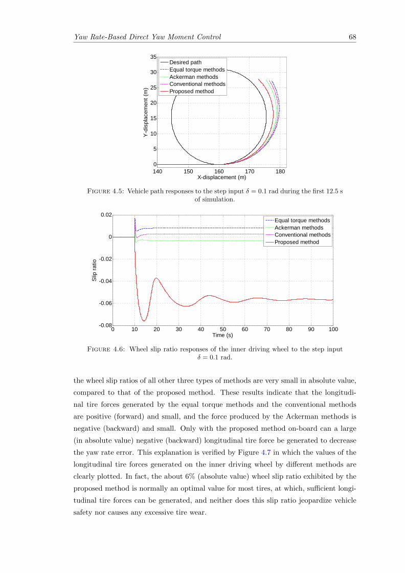
Yaw Rate-Based Direct Yaw Moment Control 68
140 150 160 170 1800
5
10
15
20
25
30
35
X-displacement (m)
Y-di
spla
cem
ent (
m)
Desired pathEqual torque methodsAckerman methodsConventional methodsProposed method
Figure 4.5: Vehicle path responses to the step input δ = 0.1 rad during the first 12.5 sof simulation.
0 10 20 30 40 50 60 70 80 90 100-0.08
-0.06
-0.04
-0.02
0
0.02
Time (s)
Slip
ratio
Equal torque methodsAckerman methodsConventional methodsProposed method
Figure 4.6: Wheel slip ratio responses of the inner driving wheel to the step inputδ = 0.1 rad.
the wheel slip ratios of all other three types of methods are very small in absolute value,
compared to that of the proposed method. These results indicate that the longitudi-
nal tire forces generated by the equal torque methods and the conventional methods
are positive (forward) and small, and the force produced by the Ackerman methods is
negative (backward) and small. Only with the proposed method on-board can a large
(in absolute value) negative (backward) longitudinal tire force be generated to decrease
the yaw rate error. This explanation is verified by Figure 4.7 in which the values of the
longitudinal tire forces generated on the inner driving wheel by different methods are
clearly plotted. In fact, the about 6% (absolute value) wheel slip ratio exhibited by the
proposed method is normally an optimal value for most tires, at which, sufficient longi-
tudinal tire forces can be generated, and neither does this slip ratio jeopardize vehicle
safety nor causes any excessive tire wear.
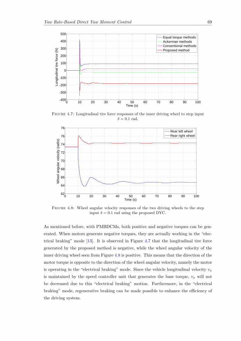
Yaw Rate-Based Direct Yaw Moment Control 69
0 10 20 30 40 50 60 70 80 90 100-400
-300
-200
-100
0
100
200
300
400
500
Time (s)
Long
itudi
nal t
ire fo
rce
(N)
Equal torque methodsAckerman methodsConventional methodsProposed method
Figure 4.7: Longitudinal tire force responses of the inner driving wheel to step inputδ = 0.1 rad.
0 10 20 30 40 50 60 70 80 90 10062
64
66
68
70
72
74
76
78
Time (s)
Whe
el a
ngul
ar v
eloc
ity (r
ad/s
)
Rear left wheelRear right wheel
Figure 4.8: Wheel angular velocity responses of the two driving wheels to the stepinput δ = 0.1 rad using the proposed DYC.
As mentioned before, with PMBDCMs, both positive and negative torques can be gen-
erated. When motors generate negative torques, they are actually working in the “elec-
trical braking” mode [13]. It is observed in Figure 4.7 that the longitudinal tire force
generated by the proposed method is negative, while the wheel angular velocity of the
inner driving wheel seen from Figure 4.8 is positive. This means that the direction of the
motor torque is opposite to the direction of the wheel angular velocity, namely the motor
is operating in the “electrical braking” mode. Since the vehicle longitudinal velocity vx
is maintained by the speed controller unit that generates the base torque, vx will not
be decreased due to this “electrical braking” motion. Furthermore, in the “electrical
braking” mode, regenerative braking can be made possible to enhance the efficiency of
the driving system.
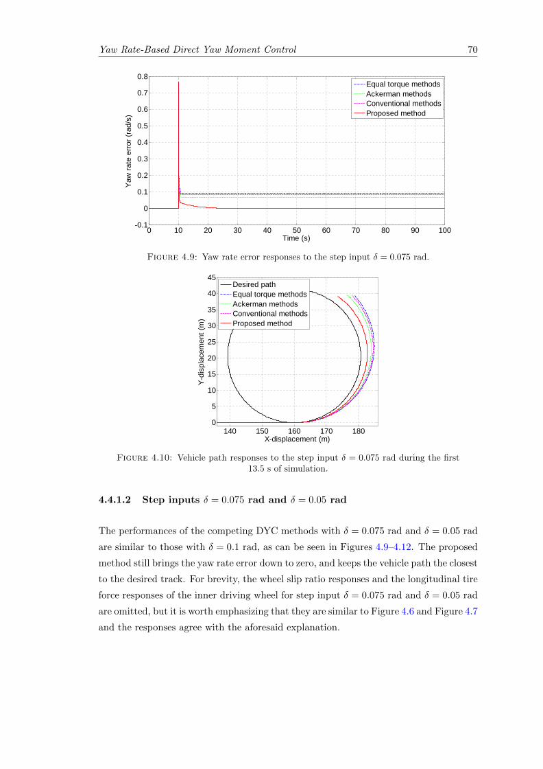
Yaw Rate-Based Direct Yaw Moment Control 70
0 10 20 30 40 50 60 70 80 90 100-0.1
0
0.1
0.2
0.3
0.4
0.5
0.6
0.7
0.8
Time (s)
Yaw
rate
erro
r (ra
d/s)
Equal torque methodsAckerman methodsConventional methodsProposed method
Figure 4.9: Yaw rate error responses to the step input δ = 0.075 rad.
140 150 160 170 1800
5
10
15
20
25
30
35
40
45
X-displacement (m)
Y-di
spla
cem
ent (
m)
Desired pathEqual torque methodsAckerman methodsConventional methodsProposed method
Figure 4.10: Vehicle path responses to the step input δ = 0.075 rad during the first13.5 s of simulation.
4.4.1.2 Step inputs δ = 0.075 rad and δ = 0.05 rad
The performances of the competing DYC methods with δ = 0.075 rad and δ = 0.05 rad
are similar to those with δ = 0.1 rad, as can be seen in Figures 4.9–4.12. The proposed
method still brings the yaw rate error down to zero, and keeps the vehicle path the closest
to the desired track. For brevity, the wheel slip ratio responses and the longitudinal tire
force responses of the inner driving wheel for step input δ = 0.075 rad and δ = 0.05 rad
are omitted, but it is worth emphasizing that they are similar to Figure 4.6 and Figure 4.7
and the responses agree with the aforesaid explanation.
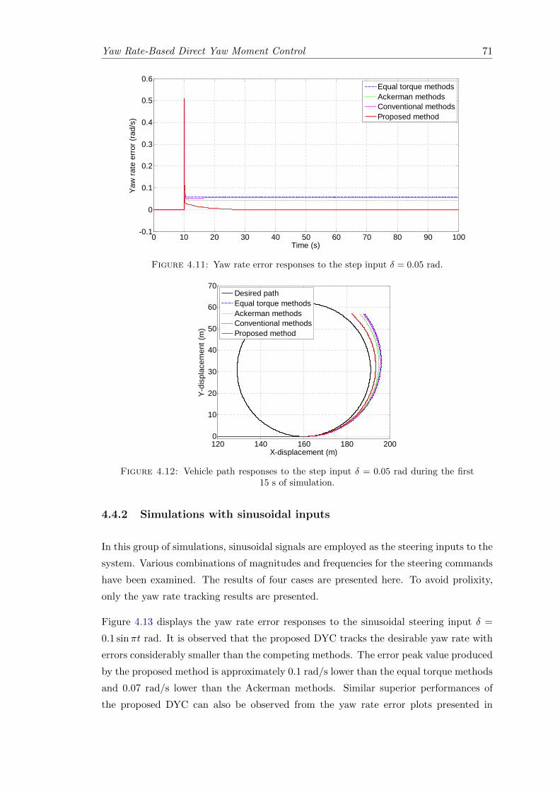
Yaw Rate-Based Direct Yaw Moment Control 71
0 10 20 30 40 50 60 70 80 90 100-0.1
0
0.1
0.2
0.3
0.4
0.5
0.6
Time (s)
Yaw
rate
erro
r (ra
d/s)
Equal torque methodsAckerman methodsConventional methodsProposed method
Figure 4.11: Yaw rate error responses to the step input δ = 0.05 rad.
120 140 160 180 2000
10
20
30
40
50
60
70
X-displacement (m)
Y-di
spla
cem
ent (
m)
Desired pathEqual torque methodsAckerman methodsConventional methodsProposed method
Figure 4.12: Vehicle path responses to the step input δ = 0.05 rad during the first15 s of simulation.
4.4.2 Simulations with sinusoidal inputs
In this group of simulations, sinusoidal signals are employed as the steering inputs to the
system. Various combinations of magnitudes and frequencies for the steering commands
have been examined. The results of four cases are presented here. To avoid prolixity,
only the yaw rate tracking results are presented.
Figure 4.13 displays the yaw rate error responses to the sinusoidal steering input δ =
0.1 sinπt rad. It is observed that the proposed DYC tracks the desirable yaw rate with
errors considerably smaller than the competing methods. The error peak value produced
by the proposed method is approximately 0.1 rad/s lower than the equal torque methods
and 0.07 rad/s lower than the Ackerman methods. Similar superior performances of
the proposed DYC can also be observed from the yaw rate error plots presented in
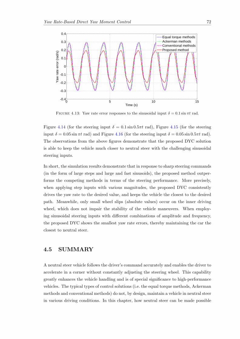
Yaw Rate-Based Direct Yaw Moment Control 72
0 5 10 15-0.4
-0.3
-0.2
-0.1
0
0.1
0.2
0.3
0.4
Time (s)
Yaw
rate
erro
r (ra
d/s)
Equal torque methodsAckerman methodsConventional methodsProposed method
Figure 4.13: Yaw rate error responses to the sinusoidal input δ = 0.1 sinπt rad.
Figure 4.14 (for the steering input δ = 0.1 sin 0.5πt rad), Figure 4.15 (for the steering
input δ = 0.05 sinπt rad) and Figure 4.16 (for the steering input δ = 0.05 sin 0.5πt rad).
The observations from the above figures demonstrate that the proposed DYC solution
is able to keep the vehicle much closer to neutral steer with the challenging sinusoidal
steering inputs.
In short, the simulation results demonstrate that in response to sharp steering commands
(in the form of large steps and large and fast sinusoids), the proposed method outper-
forms the competing methods in terms of the steering performance. More precisely,
when applying step inputs with various magnitudes, the proposed DYC consistently
drives the yaw rate to the desired value, and keeps the vehicle the closest to the desired
path. Meanwhile, only small wheel slips (absolute values) occur on the inner driving
wheel, which does not impair the stability of the vehicle maneuvers. When employ-
ing sinusoidal steering inputs with different combinations of amplitude and frequency,
the proposed DYC shows the smallest yaw rate errors, thereby maintaining the car the
closest to neutral steer.
4.5 SUMMARY
A neutral steer vehicle follows the driver’s command accurately and enables the driver to
accelerate in a corner without constantly adjusting the steering wheel. This capability
greatly enhances the vehicle handling and is of special significance to high-performance
vehicles. The typical types of control solutions (i.e. the equal torque methods, Ackerman
methods and conventional methods) do not, by design, maintain a vehicle in neutral steer
in various driving conditions. In this chapter, how neutral steer can be made possible
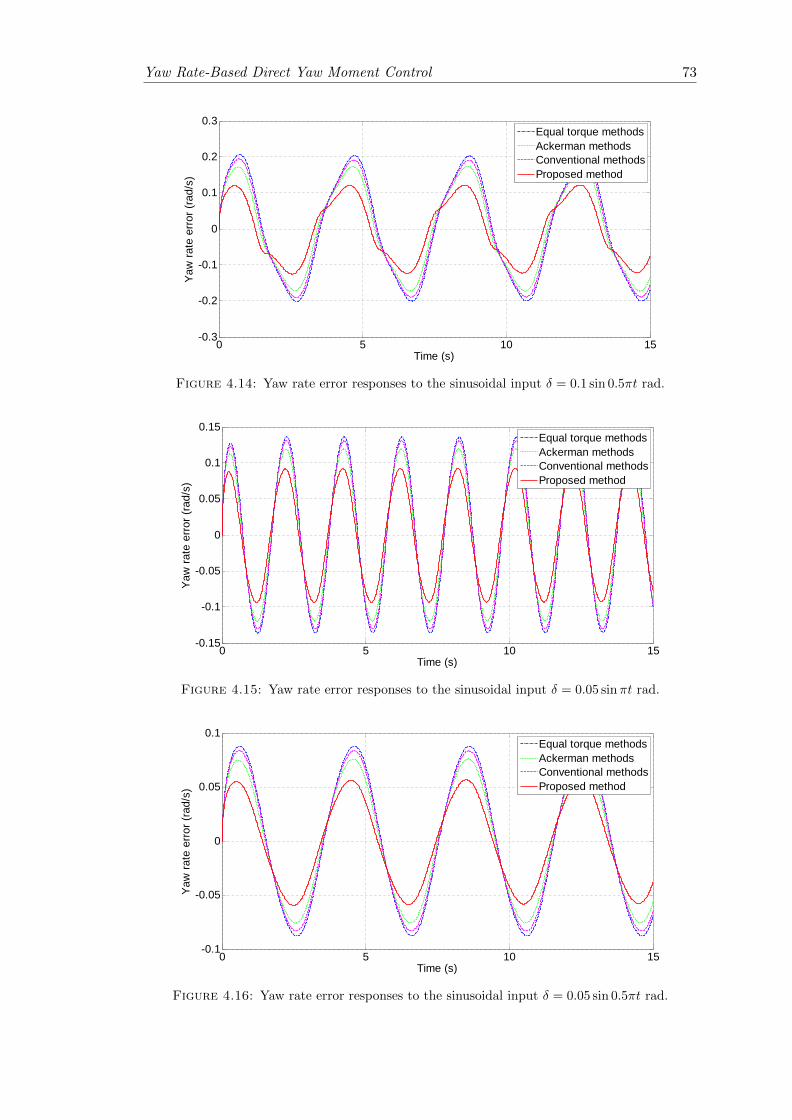
Yaw Rate-Based Direct Yaw Moment Control 73
0 5 10 15-0.3
-0.2
-0.1
0
0.1
0.2
0.3
Time (s)
Yaw
rate
erro
r (ra
d/s)
Equal torque methodsAckerman methodsConventional methodsProposed method
Figure 4.14: Yaw rate error responses to the sinusoidal input δ = 0.1 sin 0.5πt rad.
0 5 10 15-0.15
-0.1
-0.05
0
0.05
0.1
0.15
Time (s)
Yaw
rate
erro
r (ra
d/s)
Equal torque methodsAckerman methodsConventional methodsProposed method
Figure 4.15: Yaw rate error responses to the sinusoidal input δ = 0.05 sinπt rad.
0 5 10 15-0.1
-0.05
0
0.05
0.1
Time (s)
Yaw
rate
erro
r (ra
d/s)
Equal torque methodsAckerman methodsConventional methodsProposed method
Figure 4.16: Yaw rate error responses to the sinusoidal input δ = 0.05 sin 0.5πt rad.
Yaw Rate-Based Direct Yaw Moment Control 74
for vehicles with independent motors using the proposed yaw rate-based DYC system
has been mathematically and graphically demonstrated.
Simulation results manifest that with the challenging steering inputs, using the proposed
DYC method, the vehicle closely tracks the desired yaw rate that corresponds to neutral
steer, namely, a close-to-neutral steer characteristic is achieved. It is also shown in the
simulations that in various challenging steering scenarios, the proposed DYC outper-
forms the competing control solutions in terms of tracking the desired yaw rate and
desired vehicle path.
Chapter 5
Vehicle Side-Slip-Based Direct
Yaw Moment Control
In this chapter, similar to Chapter 4, a mathematical relationship is derived from a set
of simplified vehicle equations of motion. This relationship reveals that the steady-state
vehicle side-slip directly depends on the torque difference between the left and right
driving motors, therefore, it can be directly controlled by tuning this torque difference
to track a reference value. On the basis of this relationship, a vehicle side-slip-based DYC
solution is proposed to achieve zero vehicle side-slip. Simulation results manifest that
the proposed DYC method keeps the vehicle side-slip close to zero in various challenging
steering scenarios. Also, the proposed DYC solution outperforms two typical types of
control schemes in terms of the vehicle side-slip responses.
5.1 BACKGROUND
As introduced in Chapter 1, the vehicle side-slip β is the angle between the vehicle
heading direction (the positive direction of the x-axis in the vehicle local coordinate
x-y-z) and the velocity vector v of the point P, as shown in Figure 1.4. The vehicle
side-slip is also a crucial vehicle state which requires to be controlled. Ideally, it needs
to be minimized, for two reasons: Firstly, due to the nonlinear tire characteristics, as
the vehicle side-slip increases to large values, the tire cornering stiffnesses decrease and
the yaw moment generated by the lateral tire forces descends [21]. When the vehicle
side-slip is sufficiently large, the generated yaw moment becomes negligible and it can
hardly be increased by changing the steer angle. As a result, the vehicle tends to lose its
stability. Secondly, the vehicle side-slip is normally non-zero during cornering, and the
driver intuitively assumes that the vehicle heading direction is the direction where the
75
Vehicle Side-Slip-Based Direct Yaw Moment Control 76
vehicle is going. This wrong assumption can mislead the driver into performing excessive
or insufficient steering actions. A small vehicle side-slip angle implies a consistency of
the vehicle heading direction with the velocity vector v, which provides the driver with
superior sense of control during cornering [22].
In the following, a direct relationship between the steady-state vehicle side-slip and
the motor torque difference is first derived from the same simplified vehicle equations
of motion as in Chapter 4. Based on this relationship, a vehicle side-slip-based DYC
method is then devised to maintain the vehicle side-slip magnitude as small as possible.
Namely, the proposed DYC aims to maintain the vehicle heading direction consistent
with the velocity vector v. The merits of having small vehicle side-slip magnitude greatly
enhance the vehicle stability and driver’s sense of control. Besides, the proposed DYC
maintains the wheel slip ratio of the inner driving wheel at low magnitudes so that
excessive tire wear is prevented and the vehicle stability is further guaranteed.
The effectiveness of the proposed vehicle side-slip-based DYC is validated through sim-
ulation studies. Similar to Chapter 4, two typical types of control solutions, the equal
torque methods and Ackerman methods, are employed for comparison purposes in the
simulations.
5.2 VEHICLE SIDE-SLIP-BASED DYC DESIGN
5.2.1 Controller design
In Chapter 4, a vehicle control model, i.e., a set of linearized and simplified equations
of motion was derived to achieve the yaw rate-based DYC scheme. In this chapter, the
same control model is utilized again to derive the control law for the proposed vehicle
side-slip-based DYC.
In steady state, the vehicle control model can be expressed by equation (4.38), which is
rewritten as follows:
aβ ar −mvx aφ
0 mShSvx bφ
cβ cr cφ
β
r
φ
=
−aδ 0
0 0
−cδ −dr2
[δ
∆Fx
]. (5.1)
In Chapter 4, the above equation was solved for the yaw rate r. Here, solving this
equation for β leads to the following steady-state vehicle side-slip response in terms of
Vehicle Side-Slip-Based Direct Yaw Moment Control 77
the control inputs δ and ∆Fx:
β =Z3
Z0δ +
Z4
Z0∆Fx, (5.2)
where Z0 remains the same as in Chapter 4 and
Z3 = −aδbφcr + arbφcδ − bφcδmvx + aδcφmShSvx − aφcδmShSvx (5.3)
Z4 =dr2
(arbφ − bφmvx − aφmShSvx). (5.4)
Equation (5.2) shows that, similar to equation (4.39), the steady-state vehicle side-slip
directly depends on the longitudinal tire force difference ∆Fx.
Substituting equation (4.43) in equation (5.2) leads to:
β =Z3
Z0δ +
Z4
Z0R∆T. (5.5)
Equation (5.5) clearly demonstrates a direct relationship between the steady-state vehi-
cle side-slip and the difference between the two motor torques, ∆T . This implies that,
by properly controlling the two motor torques, the steady-state vehicle side-slip can be
tuned to attain its desired value.
According to equation (5.5), for a certain steer angle δ, the controller should be designed
to achieve a desired vehicle side-slip β∗ by creating a corresponding desired motor torque
difference ∆T ∗, namely:
β∗ =Z3
Z0δ +
Z4
Z0R∆T ∗. (5.6)
Equation (5.6) lays the theoretical foundation for the following controller design.
Subtracting equation (5.5) from equation (5.6) produces the following relationship ex-
pressed in terms of the errors in ∆T and β:
∆T ∗ −∆T =Z0R
Z4(β∗ − β). (5.7)
Note that the proposed DYC system is a discrete control system. The output of the
controller ∆T (k + 1) at discrete time k + 1, must be generated to make β(k) approach
β(k)∗ as soon as possible. Therefore, the proposed control strategy is to generate ∆T (k+
1) = ∆T ∗, which yields:
∆T (k + 1)−∆T (k) =Z0R
Z4(β(k)∗ − β(k)). (5.8)
Vehicle Side-Slip-Based Direct Yaw Moment Control 78
Dividing both sides by the sampling time ts leads to:
∆T (k + 1)−∆T (k)
ts=Z0R
Z4ts(β(k)∗ − β(k)). (5.9)
The sampling time ts of the control system is fairly short, so, the left-hand side of
equation (5.9) can be considered as the time-derivative of the torque difference ∆T .
Thus, integration of both sides of equation (5.9) in continuous time t provides:
∆T (t) =Z0R
Z4ts
∫ t
0eβ(τ)dτ, (5.10)
where,
eβ(τ) = β(τ)∗ − β(τ). (5.11)
As explained previously in section 5.1, the vehicle side-slip β should be minimized, which
means β(τ)∗ ≡ 0. Thus equation (5.11) reduces to:
eβ(τ) = −β(τ). (5.12)
Equation (5.10) indicates that the ideal torque difference between the two driving mo-
tors can be achieved by simply using an I controller. Similar to Chapter 4, the full
vehicle model introduced in Chapter 3 with the nonlinear vehicle equations of motion
is employed in the MATLAB/Simulink environment to produce the simulation results.
However, a set of linearized and simplified equations of motion is adopted to achieve
the above DYC design. To accommodate the modeling errors and better regulate the
vehicle side-slip, a PID type controller, instead of a simple I controller, is chosen for the
proposed vehicle side-slip-based DYC system.
5.2.2 Controller effect on yaw rate
Notice that the steady-state vehicle control model, equation (4.38), was solved in Chap-
ter 4 to achieve the steady-state yaw rate response, equation (4.44). Again, the same
equation is solved in this chapter to obtain the steady-state vehicle side-slip response,
equation (5.5).
Equations (4.44) and (5.5) imply that when ∆T is tuned to obtain a certain steady-state
vehicle side-slip, the steady-state yaw rate is also influenced, and vice versa. Therefore,
when designing a DYC system to regulate the vehicle side-slip, the control parameters
have to be carefully tuned in such a way that not only is a satisfactory vehicle side-slip
performance achieved, but also the yaw rate performance is not compromised. This tun-
ing involves appropriate trade-off between the vehicle side-slip and yaw rate responses.
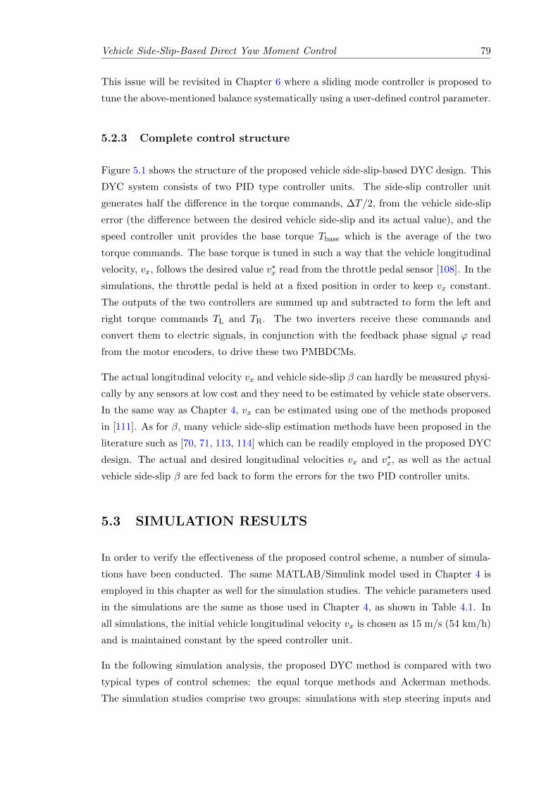
Vehicle Side-Slip-Based Direct Yaw Moment Control 79
This issue will be revisited in Chapter 6 where a sliding mode controller is proposed to
tune the above-mentioned balance systematically using a user-defined control parameter.
5.2.3 Complete control structure
Figure 5.1 shows the structure of the proposed vehicle side-slip-based DYC design. This
DYC system consists of two PID type controller units. The side-slip controller unit
generates half the difference in the torque commands, ∆T/2, from the vehicle side-slip
error (the difference between the desired vehicle side-slip and its actual value), and the
speed controller unit provides the base torque Tbase which is the average of the two
torque commands. The base torque is tuned in such a way that the vehicle longitudinal
velocity, vx, follows the desired value v∗x read from the throttle pedal sensor [108]. In the
simulations, the throttle pedal is held at a fixed position in order to keep vx constant.
The outputs of the two controllers are summed up and subtracted to form the left and
right torque commands TL and TR. The two inverters receive these commands and
convert them to electric signals, in conjunction with the feedback phase signal ϕ read
from the motor encoders, to drive these two PMBDCMs.
The actual longitudinal velocity vx and vehicle side-slip β can hardly be measured physi-
cally by any sensors at low cost and they need to be estimated by vehicle state observers.
In the same way as Chapter 4, vx can be estimated using one of the methods proposed
in [111]. As for β, many vehicle side-slip estimation methods have been proposed in the
literature such as [70, 71, 113, 114] which can be readily employed in the proposed DYC
design. The actual and desired longitudinal velocities vx and v∗x, as well as the actual
vehicle side-slip β are fed back to form the errors for the two PID controller units.
5.3 SIMULATION RESULTS
In order to verify the effectiveness of the proposed control scheme, a number of simula-
tions have been conducted. The same MATLAB/Simulink model used in Chapter 4 is
employed in this chapter as well for the simulation studies. The vehicle parameters used
in the simulations are the same as those used in Chapter 4, as shown in Table 4.1. In
all simulations, the initial vehicle longitudinal velocity vx is chosen as 15 m/s (54 km/h)
and is maintained constant by the speed controller unit.
In the following simulation analysis, the proposed DYC method is compared with two
typical types of control schemes: the equal torque methods and Ackerman methods.
The simulation studies comprise two groups: simulations with step steering inputs and
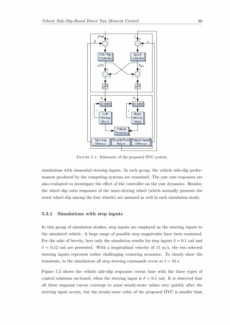
Vehicle Side-Slip-Based Direct Yaw Moment Control 80
Figure 5.1: Schematic of the proposed DYC system.
simulations with sinusoidal steering inputs. In each group, the vehicle side-slip perfor-
mances produced by the competing systems are examined. The yaw rate responses are
also evaluated to investigate the effect of the controller on the yaw dynamics. Besides,
the wheel slip ratio responses of the inner-driving wheel (which normally presents the
worst wheel slip among the four wheels) are assessed as well in each simulation study.
5.3.1 Simulations with step inputs
In this group of simulation studies, step inputs are employed as the steering inputs to
the simulated vehicle. A large range of possible step magnitudes have been examined.
For the sake of brevity, here only the simulation results for step inputs δ = 0.1 rad and
δ = 0.12 rad are presented. With a longitudinal velocity of 15 m/s, the two selected
steering inputs represent rather challenging cornering scenarios. To clearly show the
transients, in the simulations all step steering commands occur at t = 10 s.
Figure 5.2 shows the vehicle side-slip responses versus time with the three types of
control solutions on-board, when the steering input is δ = 0.1 rad. It is observed that
all three response curves converge to some steady-state values very quickly after the
steering input occurs, but the steady-state value of the proposed DYC is smaller than
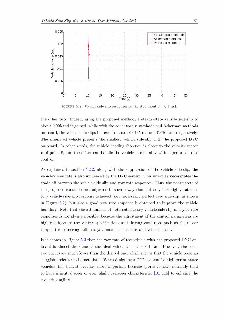
Vehicle Side-Slip-Based Direct Yaw Moment Control 81
0 5 10 15 20 25 30 35 40 45 500
0.005
0.01
0.015
0.02
0.025
Time (s)
Vehi
cle
side
-slip
(rad
)
Equal torque methodsAckerman methodsProposed method
Figure 5.2: Vehicle side-slip responses to the step input δ = 0.1 rad.
the other two. Indeed, using the proposed method, a steady-state vehicle side-slip of
about 0.005 rad is gained, while with the equal torque methods and Ackerman methods
on-board, the vehicle side-slips increase to about 0.0135 rad and 0.016 rad, respectively.
The simulated vehicle presents the smallest vehicle side-slip with the proposed DYC
on-board. In other words, the vehicle heading direction is closer to the velocity vector
v of point P, and the driver can handle the vehicle more stably with superior sense of
control.
As explained in section 5.2.2, along with the suppression of the vehicle side-slip, the
vehicle’s yaw rate is also influenced by the DYC system. This interplay necessitates the
trade-off between the vehicle side-slip and yaw rate responses. Thus, the parameters of
the proposed controller are adjusted in such a way that not only is a highly satisfac-
tory vehicle side-slip response achieved (not necessarily perfect zero side-slip, as shown
in Figure 5.2), but also a good yaw rate response is obtained to improve the vehicle
handling. Note that the attainment of both satisfactory vehicle side-slip and yaw rate
responses is not always possible, because the adjustment of the control parameters are
highly subject to the vehicle specifications and driving conditions such as the motor
torque, tire cornering stiffness, yaw moment of inertia and vehicle speed.
It is shown in Figure 5.3 that the yaw rate of the vehicle with the proposed DYC on-
board is almost the same as the ideal value, when δ = 0.1 rad. However, the other
two curves are much lower than the desired one, which means that the vehicle presents
sluggish understeer characteristic. When designing a DYC system for high-performance
vehicles, this benefit becomes more important because sports vehicles normally tend
to have a neutral steer or even slight oversteer characteristic [16, 115] to enhance the
cornering agility.
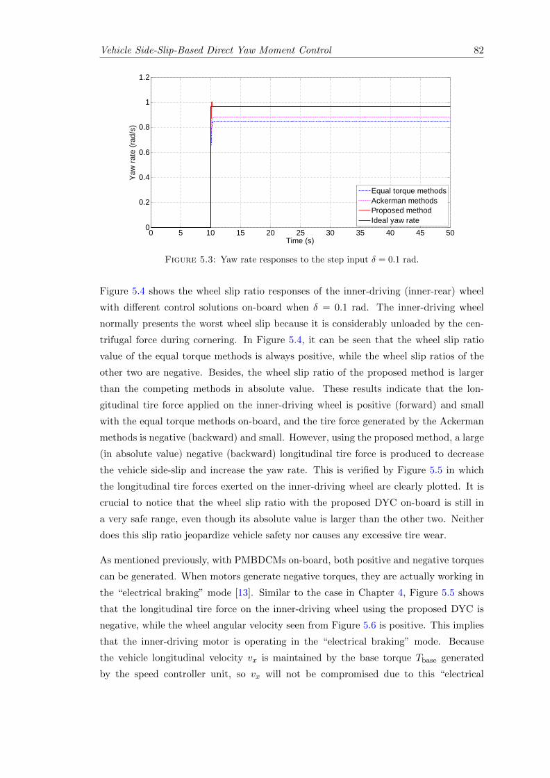
Vehicle Side-Slip-Based Direct Yaw Moment Control 82
0 5 10 15 20 25 30 35 40 45 500
0.2
0.4
0.6
0.8
1
1.2
Time (s)
Yaw
rate
(rad
/s)
Equal torque methodsAckerman methodsProposed methodIdeal yaw rate
Figure 5.3: Yaw rate responses to the step input δ = 0.1 rad.
Figure 5.4 shows the wheel slip ratio responses of the inner-driving (inner-rear) wheel
with different control solutions on-board when δ = 0.1 rad. The inner-driving wheel
normally presents the worst wheel slip because it is considerably unloaded by the cen-
trifugal force during cornering. In Figure 5.4, it can be seen that the wheel slip ratio
value of the equal torque methods is always positive, while the wheel slip ratios of the
other two are negative. Besides, the wheel slip ratio of the proposed method is larger
than the competing methods in absolute value. These results indicate that the lon-
gitudinal tire force applied on the inner-driving wheel is positive (forward) and small
with the equal torque methods on-board, and the tire force generated by the Ackerman
methods is negative (backward) and small. However, using the proposed method, a large
(in absolute value) negative (backward) longitudinal tire force is produced to decrease
the vehicle side-slip and increase the yaw rate. This is verified by Figure 5.5 in which
the longitudinal tire forces exerted on the inner-driving wheel are clearly plotted. It is
crucial to notice that the wheel slip ratio with the proposed DYC on-board is still in
a very safe range, even though its absolute value is larger than the other two. Neither
does this slip ratio jeopardize vehicle safety nor causes any excessive tire wear.
As mentioned previously, with PMBDCMs on-board, both positive and negative torques
can be generated. When motors generate negative torques, they are actually working in
the “electrical braking” mode [13]. Similar to the case in Chapter 4, Figure 5.5 shows
that the longitudinal tire force on the inner-driving wheel using the proposed DYC is
negative, while the wheel angular velocity seen from Figure 5.6 is positive. This implies
that the inner-driving motor is operating in the “electrical braking” mode. Because
the vehicle longitudinal velocity vx is maintained by the base torque Tbase generated
by the speed controller unit, so vx will not be compromised due to this “electrical
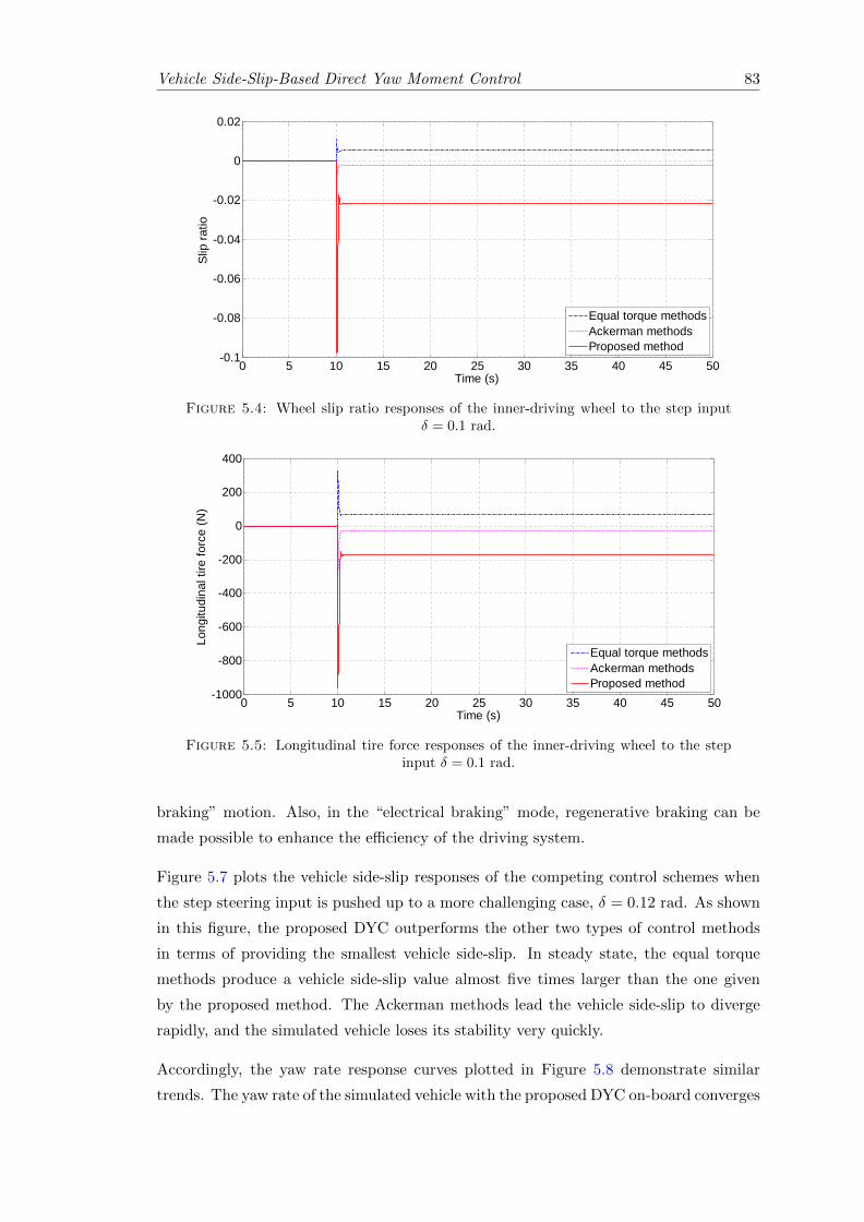
Vehicle Side-Slip-Based Direct Yaw Moment Control 83
0 5 10 15 20 25 30 35 40 45 50-0.1
-0.08
-0.06
-0.04
-0.02
0
0.02
Time (s)
Slip
ratio
Equal torque methodsAckerman methodsProposed method
Figure 5.4: Wheel slip ratio responses of the inner-driving wheel to the step inputδ = 0.1 rad.
0 5 10 15 20 25 30 35 40 45 50-1000
-800
-600
-400
-200
0
200
400
Time (s)
Long
itudi
nal t
ire fo
rce
(N)
Equal torque methodsAckerman methodsProposed method
Figure 5.5: Longitudinal tire force responses of the inner-driving wheel to the stepinput δ = 0.1 rad.
braking” motion. Also, in the “electrical braking” mode, regenerative braking can be
made possible to enhance the efficiency of the driving system.
Figure 5.7 plots the vehicle side-slip responses of the competing control schemes when
the step steering input is pushed up to a more challenging case, δ = 0.12 rad. As shown
in this figure, the proposed DYC outperforms the other two types of control methods
in terms of providing the smallest vehicle side-slip. In steady state, the equal torque
methods produce a vehicle side-slip value almost five times larger than the one given
by the proposed method. The Ackerman methods lead the vehicle side-slip to diverge
rapidly, and the simulated vehicle loses its stability very quickly.
Accordingly, the yaw rate response curves plotted in Figure 5.8 demonstrate similar
trends. The yaw rate of the simulated vehicle with the proposed DYC on-board converges
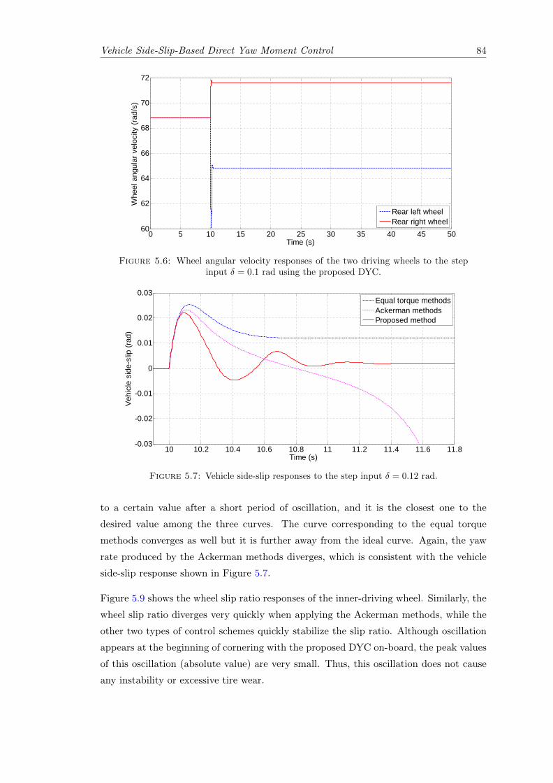
Vehicle Side-Slip-Based Direct Yaw Moment Control 84
0 5 10 15 20 25 30 35 40 45 5060
62
64
66
68
70
72
Time (s)
Whe
el a
ngul
ar v
eloc
ity (r
ad/s
)
Rear left wheelRear right wheel
Figure 5.6: Wheel angular velocity responses of the two driving wheels to the stepinput δ = 0.1 rad using the proposed DYC.
10 10.2 10.4 10.6 10.8 11 11.2 11.4 11.6 11.8-0.03
-0.02
-0.01
0
0.01
0.02
0.03
Time (s)
Vehi
cle
side
-slip
(rad
)
Equal torque methodsAckerman methodsProposed method
Figure 5.7: Vehicle side-slip responses to the step input δ = 0.12 rad.
to a certain value after a short period of oscillation, and it is the closest one to the
desired value among the three curves. The curve corresponding to the equal torque
methods converges as well but it is further away from the ideal curve. Again, the yaw
rate produced by the Ackerman methods diverges, which is consistent with the vehicle
side-slip response shown in Figure 5.7.
Figure 5.9 shows the wheel slip ratio responses of the inner-driving wheel. Similarly, the
wheel slip ratio diverges very quickly when applying the Ackerman methods, while the
other two types of control schemes quickly stabilize the slip ratio. Although oscillation
appears at the beginning of cornering with the proposed DYC on-board, the peak values
of this oscillation (absolute value) are very small. Thus, this oscillation does not cause
any instability or excessive tire wear.
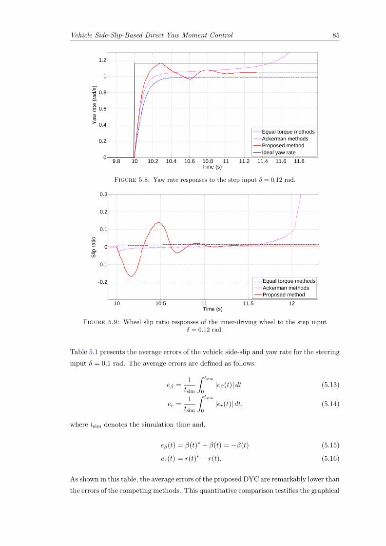
Vehicle Side-Slip-Based Direct Yaw Moment Control 85
9.8 10 10.2 10.4 10.6 10.8 11 11.2 11.4 11.6 11.80
0.2
0.4
0.6
0.8
1
1.2
Time (s)
Yaw
rate
(rad
/s)
Equal torque methodsAckerman methodsProposed methodIdeal yaw rate
Figure 5.8: Yaw rate responses to the step input δ = 0.12 rad.
10 10.5 11 11.5 12
-0.2
-0.1
0
0.1
0.2
0.3
Time (s)
Slip
ratio
Equal torque methodsAckerman methodsProposed method
Figure 5.9: Wheel slip ratio responses of the inner-driving wheel to the step inputδ = 0.12 rad.
Table 5.1 presents the average errors of the vehicle side-slip and yaw rate for the steering
input δ = 0.1 rad. The average errors are defined as follows:
eβ =1
tsim
∫ tsim
0|eβ(t)| dt (5.13)
er =1
tsim
∫ tsim
0|er(t)| dt, (5.14)
where tsim denotes the simulation time and,
eβ(t) = β(t)∗ − β(t) = −β(t) (5.15)
er(t) = r(t)∗ − r(t). (5.16)
As shown in this table, the average errors of the proposed DYC are remarkably lower than
the errors of the competing methods. This quantitative comparison testifies the graphical
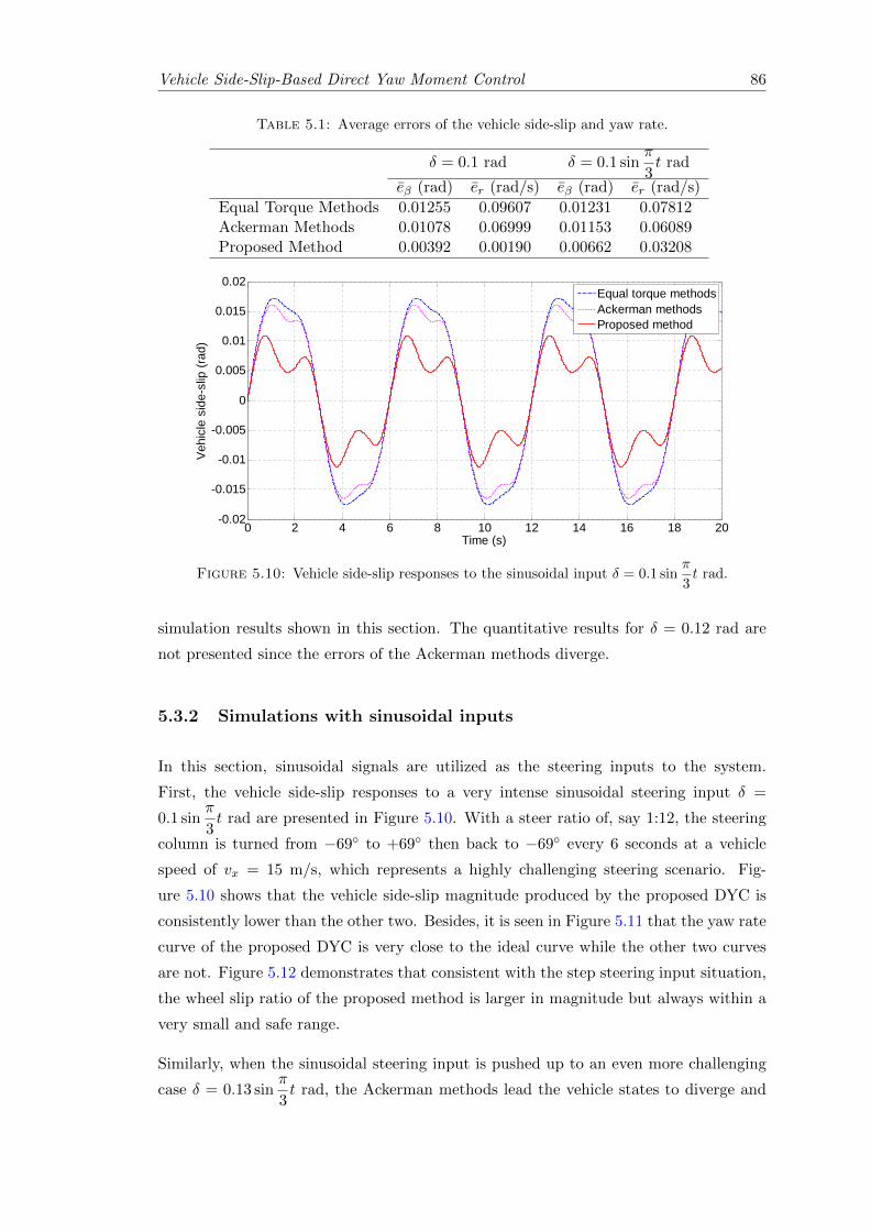
Vehicle Side-Slip-Based Direct Yaw Moment Control 86
Table 5.1: Average errors of the vehicle side-slip and yaw rate.
δ = 0.1 rad δ = 0.1 sinπ
3t rad
eβ (rad) er (rad/s) eβ (rad) er (rad/s)
Equal Torque Methods 0.01255 0.09607 0.01231 0.07812Ackerman Methods 0.01078 0.06999 0.01153 0.06089Proposed Method 0.00392 0.00190 0.00662 0.03208
0 2 4 6 8 10 12 14 16 18 20-0.02
-0.015
-0.01
-0.005
0
0.005
0.01
0.015
0.02
Time (s)
Vehi
cle
side
-slip
(rad
)
Equal torque methodsAckerman methodsProposed method
Figure 5.10: Vehicle side-slip responses to the sinusoidal input δ = 0.1 sinπ
3t rad.
simulation results shown in this section. The quantitative results for δ = 0.12 rad are
not presented since the errors of the Ackerman methods diverge.
5.3.2 Simulations with sinusoidal inputs
In this section, sinusoidal signals are utilized as the steering inputs to the system.
First, the vehicle side-slip responses to a very intense sinusoidal steering input δ =
0.1 sinπ
3t rad are presented in Figure 5.10. With a steer ratio of, say 1:12, the steering
column is turned from −69◦ to +69◦ then back to −69◦ every 6 seconds at a vehicle
speed of vx = 15 m/s, which represents a highly challenging steering scenario. Fig-
ure 5.10 shows that the vehicle side-slip magnitude produced by the proposed DYC is
consistently lower than the other two. Besides, it is seen in Figure 5.11 that the yaw rate
curve of the proposed DYC is very close to the ideal curve while the other two curves
are not. Figure 5.12 demonstrates that consistent with the step steering input situation,
the wheel slip ratio of the proposed method is larger in magnitude but always within a
very small and safe range.
Similarly, when the sinusoidal steering input is pushed up to an even more challenging
case δ = 0.13 sinπ
3t rad, the Ackerman methods lead the vehicle states to diverge and
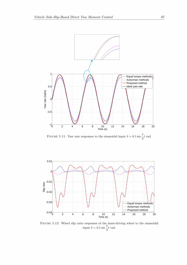
Vehicle Side-Slip-Based Direct Yaw Moment Control 87
0 2 4 6 8 10 12 14 16 18 20-1
-0.5
0
0.5
1
Time (s)
Yaw
rat
e (r
ad/s
)
Equal torque methodsAckerman methodsProposed methodIdeal yaw rate
Figure 5.11: Yaw rate responses to the sinusoidal input δ = 0.1 sinπ
3t rad.
0 2 4 6 8 10 12 14 16 18 20-0.04
-0.03
-0.02
-0.01
0
0.01
Time (s)
Slip
ratio
Equal torque methodsAckerman methodsProposed method
Figure 5.12: Wheel slip ratio responses of the inner-driving wheel to the sinusoidal
input δ = 0.1 sinπ
3t rad.
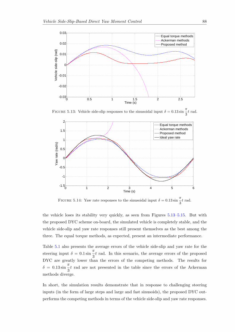
Vehicle Side-Slip-Based Direct Yaw Moment Control 88
0 0.5 1 1.5 2 2.5-0.03
-0.02
-0.01
0
0.01
0.02
0.03
Time (s)
Vehi
cle
side
-slip
(rad
)
Equal torque methodsAckerman methodsProposed method
Figure 5.13: Vehicle side-slip responses to the sinusoidal input δ = 0.13 sinπ
3t rad.
0 1 2 3 4 5 6-1.5
-1
-0.5
0
0.5
1
1.5
2
Time (s)
Yaw
rate
(rad
/s)
Equal torque methodsAckerman methodsProposed methodIdeal yaw rate
Figure 5.14: Yaw rate responses to the sinusoidal input δ = 0.13 sinπ
3t rad.
the vehicle loses its stability very quickly, as seen from Figures 5.13–5.15. But with
the proposed DYC scheme on-board, the simulated vehicle is completely stable, and the
vehicle side-slip and yaw rate responses still present themselves as the best among the
three. The equal torque methods, as expected, present an intermediate performance.
Table 5.1 also presents the average errors of the vehicle side-slip and yaw rate for the
steering input δ = 0.1 sinπ
3t rad. In this scenario, the average errors of the proposed
DYC are greatly lower than the errors of the competing methods. The results for
δ = 0.13 sinπ
3t rad are not presented in the table since the errors of the Ackerman
methods diverge.
In short, the simulation results demonstrate that in response to challenging steering
inputs (in the form of large steps and large and fast sinusoids), the proposed DYC out-
performs the competing methods in terms of the vehicle side-slip and yaw rate responses.
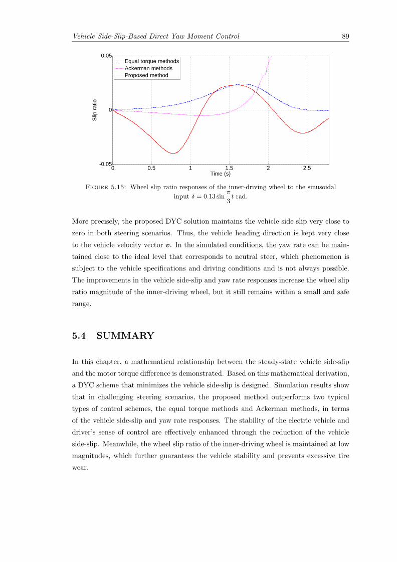
Vehicle Side-Slip-Based Direct Yaw Moment Control 89
0 0.5 1 1.5 2 2.5-0.05
0
0.05
Time (s)
Slip
ratio
Equal torque methodsAckerman methodsProposed method
Figure 5.15: Wheel slip ratio responses of the inner-driving wheel to the sinusoidal
input δ = 0.13 sinπ
3t rad.
More precisely, the proposed DYC solution maintains the vehicle side-slip very close to
zero in both steering scenarios. Thus, the vehicle heading direction is kept very close
to the vehicle velocity vector v. In the simulated conditions, the yaw rate can be main-
tained close to the ideal level that corresponds to neutral steer, which phenomenon is
subject to the vehicle specifications and driving conditions and is not always possible.
The improvements in the vehicle side-slip and yaw rate responses increase the wheel slip
ratio magnitude of the inner-driving wheel, but it still remains within a small and safe
range.
5.4 SUMMARY
In this chapter, a mathematical relationship between the steady-state vehicle side-slip
and the motor torque difference is demonstrated. Based on this mathematical derivation,
a DYC scheme that minimizes the vehicle side-slip is designed. Simulation results show
that in challenging steering scenarios, the proposed method outperforms two typical
types of control schemes, the equal torque methods and Ackerman methods, in terms
of the vehicle side-slip and yaw rate responses. The stability of the electric vehicle and
driver’s sense of control are effectively enhanced through the reduction of the vehicle
side-slip. Meanwhile, the wheel slip ratio of the inner-driving wheel is maintained at low
magnitudes, which further guarantees the vehicle stability and prevents excessive tire
wear.
Chapter 6
Simultaneous Control of Yaw
Rate and Vehicle Side-Slip
The potential problems of controlling one vehicle state only (either the yaw rate or vehicle
side-slip) have been pointed out in section 2.5.1. To eliminate the potential downsides
and combine the benefits of controlling the yaw rate and vehicle side-slip individually,
numerous recent DYC designs adopt both states simultaneously as the control variables.
In these works, the sliding mode control technique is commonly employed to generate
the target yaw moment. This chapter proposes a new sliding mode-based DYC method
for tracking both the desired yaw rate and vehicle side-slip. This DYC scheme employs
a novel switching function, a linear combination of the normalized absolute values of the
yaw rate and vehicle side-slip errors, to guarantee the simultaneous convergences of both
vehicle states. Also, instead of the linearized and simplified vehicle control model, the
complete nonlinear vehicle equations of motion established in Chapter 3 are employed
in the control system design, which helps to construct a more effective control law.
Comparative simulation results demonstrate that the proposed DYC design outperforms
the competing methods in terms of tracking the reference yaw rate, vehicle path and
vehicle side-slip in various challenging driving scenarios.
6.1 BACKGROUND
As shown in the preceding chapters, the yaw rate and vehicle side-slip present themselves
as the fundamental states that govern the vehicle handling and stability. In Chapters 4
and 5, two DYC system for controlling the yaw rate or vehicle side-slip individually are
proposed. However, the improvements in control performance by taking into account
both vehicle states have not been discussed yet so far. In this chapter, a new sliding mode
90
Simultaneous Control of Yaw Rate and Vehicle Side-Slip 91
control scheme is proposed to regulate the yaw rate and vehicle side-slip simultaneously,
aiming at eliminating the imperfections and limitations of the existing sliding mode-
based DYC systems.
A vehicle is a nonlinear system which undergoes various ambient disturbances. Be-
sides, the vehicle models are never perfectly accurate and some model uncertainties are
always present. Since the sliding mode control technique provides robustness against
disturbances and uncertainties when controlling nonlinear systems [75–77], it is widely
used in vehicle stability and handling control and has become the most popular control
technique in the latest DYC solutions.
In the recent DYC solutions, the most common sliding mode control design employs a
linear combination of the yaw rate and vehicle side-slip errors as the switching function
which takes the following form [17, 23, 24, 78–81]:
s = r − r∗ + ξ(β − β∗), (6.1)
where r∗ and β∗ are the same desired (reference) yaw rate and vehicle side-slip as in
Chapters 4 and 5, and ξ is a positive design parameter.
The above popular switching function presents two limitations. Firstly, in some certain
circumstances, this switching function cannot guarantee simultaneous convergences of
both errors to zero. In sliding mode control, the objective is to drive the system trajec-
tories towards the sliding surface s = 0 and then maintain the trajectories on it. With
the above switching function, if the yaw rate error r − r∗ and the vehicle side-slip error
β − β∗ have the same sign, when the sliding surface s = 0 is reached, these two errors
are guaranteed to vanish. However, since the signs of the errors may change in various
driving conditions, s = 0 can also hold when one error is positive and the other is nega-
tive with the right ξ. As a result, the sliding mode controller may fail. This limitation
is exposed in a simulation case study in Section 6.3 where the two errors present oppo-
site signs and the common sliding mode controller using the above switching function
produces inferior control performance to the competing methods. Secondly, the design
parameter ξ, intuitively, is expected to represent the emphasis between the two error
terms. However, the yaw rate error r − r∗ and the vehicle side-slip error β − β∗ have
different dimensions. In order for the addition in equation (6.1) to be valid, the param-
eter ξ cannot be dimensionless. Thus, it cannot represent the emphasis between the two
errors. These two limitations may jeopardize the robustness of DYC systems and bring
about confusions in the course of DYC design.
Many existing DYC solutions (e.g. [23, 51, 66, 79]) are designed based on the well-known
two DoF bicycle model [20] and/or linear tire model [116], which neglect the vehicle roll
Simultaneous Control of Yaw Rate and Vehicle Side-Slip 92
motion and tire cornering stiffness nonlinearity, respectively. In high lateral acceleration
scenarios, significant vehicle body roll and lateral load transfer lead to the change of tire
cornering stiffnesses and in turn, vehicle dynamics. Thus, the bicycle model and linear
tire model cannot accurately describe the vehicle responses in high lateral acceleration
scenarios [116]. As a result, the control systems based on such models may produce
unexpected vehicle responses [109].
In this chapter, the complete nonlinear vehicle equations of motion derived in Chapter 3
are used to devise a novel sliding mode DYC method. The proposed DYC scheme is
designed based on a new switching function, a linear combination of the normalized abso-
lute values of the yaw rate and vehicle side-slip errors, to eliminate the above-mentioned
limitations with the commonly used switching function, equation (6.1). Extensive com-
parative simulations show that the proposed DYC solution outperforms the competing
methods in terms of tracking the desired (reference) yaw rate, vehicle path and vehicle
side-slip in different challenging driving scenarios.
6.2 PROPOSED DYC DESIGN
In this section, a DYC system based on sliding mode control is designed to track the
desired yaw rate and vehicle side-slip simultaneously. The same desired (reference) yaw
rate and vehicle side-slip used in Chapters 4 and 5 are employed, which are rewritten as
follows:
r∗ =vxlδ (6.2)
β∗ = 0. (6.3)
As mentioned in Chapter 4, δ is computed from the reading of a steering wheel angle
sensor, and vx can be estimated using one of the methods proposed in [111]. Note that
these desired values can be altered according to the driver’s preference, which does not
change the basic properties of the proposed controller.
The control objective is to track the desired yaw rate and vehicle side-slip simultaneously.
To achieve this goal by means of sliding mode control, one critical step is to appropri-
ately design a switching function. In this design, instead of equation (6.1), a linear
combination of the normalized absolute values of errors is proposed as the switching
function:
s =ρ
|∆r|max|r − r∗|+ 1− ρ
|∆β|max|β − β∗|, (6.4)
Simultaneous Control of Yaw Rate and Vehicle Side-Slip 93
where ρ ∈ [0, 1] is a design parameter, and |∆r|max and |∆β|max are the maximum
absolute values of the yaw rate error and vehicle side-slip error defined by the designer,
respectively.
Due to the absolute values, the proposed switching function (6.4) becomes zero only
when r converges to r∗ and β converges to β∗ simultaneously, regardless of the signs of
the yaw rate and vehicle side-slip errors. Besides, the two error terms are normalized,
so the design parameter ρ is dimensionless and it represents the emphasis on the yaw
rate error (while 1− ρ represents the emphasis on the vehicle side-slip error).
Since the target vehicle side-slip is zero, equation (6.4) reduces to:
s =ρ
|∆r|max|r − r∗|+ 1− ρ
|β|max|β|, (6.5)
and the derivative of the switching function (6.5) is given by:
s =ρ
|∆r|max(r − r∗) sgn(r − r∗) +
1− ρ|β|max
β sgn(β). (6.6)
Following the fundamental principle in sliding mode control, to drive the system trajec-
tories to the sliding surface s = 0, the following sliding condition should be satisfied [77]:
1
2
d
dts2 = ss 6 −η|s|, (6.7)
where η is a strictly positive constant. Since outside the sliding surface, s > 0, the above
condition simplifies to:
s 6 −η. (6.8)
In order to investigate s, according to equation (6.6), the expression of the yaw accel-
eration r is required. Rearrangement of equation (3.72) yields the following expression
for r:
r =1
Iz
(Ixz p+
4∑i=1
xi(Fxi sin δi + Fyi cos δi)−2∑i=1
yi(Fxi cos δi − Fyi sin δi) + ∆M), (6.9)
with ∆M =dr2
(Fx3 − Fx4). Note that this ∆M is the yaw moment generated by the
difference between the rear longitudinal tire forces.
To satisfy the sliding condition (6.8), the following corrective yaw moment command is
proposed as the control input to the vehicle system:
∆M = ∆Meq − k sgn(r − r∗), (6.10)
Simultaneous Control of Yaw Rate and Vehicle Side-Slip 94
where k is a design parameter, and ∆Meq is the term called “equivalent control” in the
sliding mode control theory. In this application, ∆Meq is given by:
∆Meq = Iz
(r∗ − |∆r|max
|β|max
1− ρρ
β sgn((r − r∗)β
))
−4∑i=1
xi(Fxi sin δi + Fyi cos δi) +2∑i=1
yi(Fxi cos δi − Fyi sin δi). (6.11)
This ∆Meq would maintain s = 0 if all states in expression (6.11) were exactly known.
Substituting the above control input ∆M in equation (6.9), and substituting the result-
ing r in equation (6.6), the following expression for s can be derived:
s =ρ
Iz|∆r|max
(f sgn(r − r∗)− k
), (6.12)
with f = Ixz p. Substituting equation (6.12) in the sliding condition (6.8) necessitates
the design parameter k to satisfy:
k > f sgn(r − r∗) +ηIz|∆r|max
ρ. (6.13)
Since Ixz is constant and the roll acceleration p is practically constrained, it can be
assumed that the term f is bounded, i.e. |f | 6 Ixz pmax. In practice, a user-defined
constant bound F > Ixz pmax is applied. Therefore, to guarantee that the above condition
(hence the sliding condition) is met, k can be chosen as:
k = F +ηIz|∆r|max
ρ. (6.14)
The computation of the proposed control input ∆M requires the knowledge of some
vehicle states including the yaw rate, vehicle side-slip and tire forces. The yaw rate
can be measured by an on-board gyroscope with reasonable accuracy, and the vehicle
side-slip can be estimated using one of the techniques proposed in [69–74]. Besides, the
estimation of tire forces is addressed in [69, 70, 100, 101].
It is important to note that the measurement or estimation errors can be compensated
for by appropriately increasing the chosen value of F . How this is the case for the force
estimation error is shown in the following. Denoting the estimated longitudinal and
lateral tire forces of the ith wheel by Fxi and Fyi, respectively, the equivalent control
∆Meq is computed as follows:
∆Meq = Iz
(r∗ − |∆r|max
|β|max
1− ρρ
β sgn((r − r∗)β
))
−4∑i=1
xi(Fxi sin δi + Fyi cos δi) +2∑i=1
yi(Fxi cos δi − Fyi sin δi), (6.15)
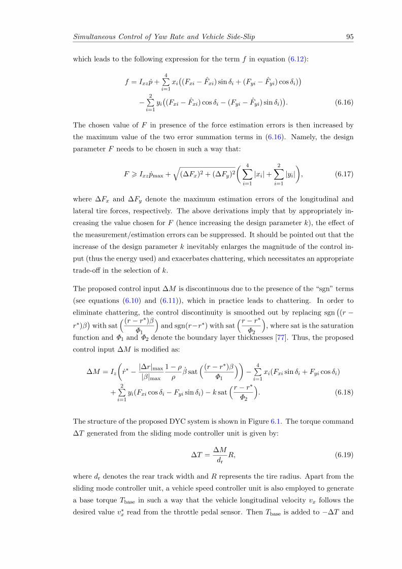
Simultaneous Control of Yaw Rate and Vehicle Side-Slip 95
which leads to the following expression for the term f in equation (6.12):
f = Ixz p+4∑i=1
xi((Fxi − Fxi) sin δi + (Fyi − Fyi) cos δi)
)
−2∑i=1
yi((Fxi − Fxi) cos δi − (Fyi − Fyi) sin δi)
). (6.16)
The chosen value of F in presence of the force estimation errors is then increased by
the maximum value of the two error summation terms in (6.16). Namely, the design
parameter F needs to be chosen in such a way that:
F > Ixz pmax +√
(∆Fx)2 + (∆Fy)2( 4∑
i=1
|xi|+2∑
i=1
|yi|), (6.17)
where ∆Fx and ∆Fy denote the maximum estimation errors of the longitudinal and
lateral tire forces, respectively. The above derivations imply that by appropriately in-
creasing the value chosen for F (hence increasing the design parameter k), the effect of
the measurement/estimation errors can be suppressed. It should be pointed out that the
increase of the design parameter k inevitably enlarges the magnitude of the control in-
put (thus the energy used) and exacerbates chattering, which necessitates an appropriate
trade-off in the selection of k.
The proposed control input ∆M is discontinuous due to the presence of the “sgn” terms
(see equations (6.10) and (6.11)), which in practice leads to chattering. In order to
eliminate chattering, the control discontinuity is smoothed out by replacing sgn((r −
r∗)β)
with sat((r − r∗)β
Φ1
)and sgn(r−r∗) with sat
(r − r∗Φ2
), where sat is the saturation
function and Φ1 and Φ2 denote the boundary layer thicknesses [77]. Thus, the proposed
control input ∆M is modified as:
∆M = Iz
(r∗ − |∆r|max
|β|max
1− ρρ
β sat((r − r∗)β
Φ1
))−
4∑i=1
xi(Fxi sin δi + Fyi cos δi)
+2∑i=1
yi(Fxi cos δi − Fyi sin δi)− k sat(r − r∗
Φ2
). (6.18)
The structure of the proposed DYC system is shown in Figure 6.1. The torque command
∆T generated from the sliding mode controller unit is given by:
∆T =∆M
drR, (6.19)
where dr denotes the rear track width and R represents the tire radius. Apart from the
sliding mode controller unit, a vehicle speed controller unit is also employed to generate
a base torque Tbase in such a way that the vehicle longitudinal velocity vx follows the
desired value v∗x read from the throttle pedal sensor. Then Tbase is added to −∆T and
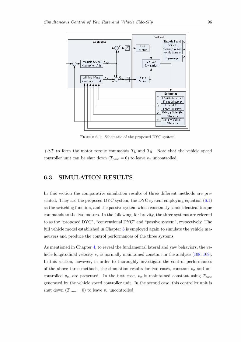
Simultaneous Control of Yaw Rate and Vehicle Side-Slip 96
Figure 6.1: Schematic of the proposed DYC system.
+∆T to form the motor torque commands TL and TR. Note that the vehicle speed
controller unit can be shut down (Tbase = 0) to leave vx uncontrolled.
6.3 SIMULATION RESULTS
In this section the comparative simulation results of three different methods are pre-
sented. They are the proposed DYC system, the DYC system employing equation (6.1)
as the switching function, and the passive system which constantly sends identical torque
commands to the two motors. In the following, for brevity, the three systems are referred
to as the “proposed DYC”, “conventional DYC” and “passive system”, respectively. The
full vehicle model established in Chapter 3 is employed again to simulate the vehicle ma-
neuvers and produce the control performances of the three systems.
As mentioned in Chapter 4, to reveal the fundamental lateral and yaw behaviors, the ve-
hicle longitudinal velocity vx is normally maintained constant in the analysis [108, 109].
In this section, however, in order to thoroughly investigate the control performances
of the above three methods, the simulation results for two cases, constant vx and un-
controlled vx, are presented. In the first case, vx is maintained constant using Tbase
generated by the vehicle speed controller unit. In the second case, this controller unit is
shut down (Tbase = 0) to leave vx uncontrolled.
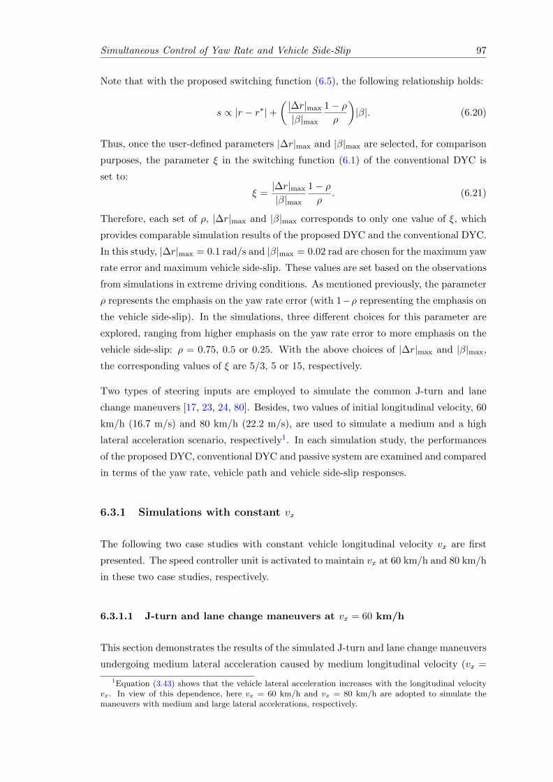
Simultaneous Control of Yaw Rate and Vehicle Side-Slip 97
Note that with the proposed switching function (6.5), the following relationship holds:
s ∝ |r − r∗|+( |∆r|max
|β|max
1− ρρ
)|β|. (6.20)
Thus, once the user-defined parameters |∆r|max and |β|max are selected, for comparison
purposes, the parameter ξ in the switching function (6.1) of the conventional DYC is
set to:
ξ =|∆r|max
|β|max
1− ρρ
. (6.21)
Therefore, each set of ρ, |∆r|max and |β|max corresponds to only one value of ξ, which
provides comparable simulation results of the proposed DYC and the conventional DYC.
In this study, |∆r|max = 0.1 rad/s and |β|max = 0.02 rad are chosen for the maximum yaw
rate error and maximum vehicle side-slip. These values are set based on the observations
from simulations in extreme driving conditions. As mentioned previously, the parameter
ρ represents the emphasis on the yaw rate error (with 1−ρ representing the emphasis on
the vehicle side-slip). In the simulations, three different choices for this parameter are
explored, ranging from higher emphasis on the yaw rate error to more emphasis on the
vehicle side-slip: ρ = 0.75, 0.5 or 0.25. With the above choices of |∆r|max and |β|max,
the corresponding values of ξ are 5/3, 5 or 15, respectively.
Two types of steering inputs are employed to simulate the common J-turn and lane
change maneuvers [17, 23, 24, 80]. Besides, two values of initial longitudinal velocity, 60
km/h (16.7 m/s) and 80 km/h (22.2 m/s), are used to simulate a medium and a high
lateral acceleration scenario, respectively1. In each simulation study, the performances
of the proposed DYC, conventional DYC and passive system are examined and compared
in terms of the yaw rate, vehicle path and vehicle side-slip responses.
6.3.1 Simulations with constant vx
The following two case studies with constant vehicle longitudinal velocity vx are first
presented. The speed controller unit is activated to maintain vx at 60 km/h and 80 km/h
in these two case studies, respectively.
6.3.1.1 J-turn and lane change maneuvers at vx = 60 km/h
This section demonstrates the results of the simulated J-turn and lane change maneuvers
undergoing medium lateral acceleration caused by medium longitudinal velocity (vx =
1Equation (3.43) shows that the vehicle lateral acceleration increases with the longitudinal velocityvx. In view of this dependence, here vx = 60 km/h and vx = 80 km/h are adopted to simulate themaneuvers with medium and large lateral accelerations, respectively.
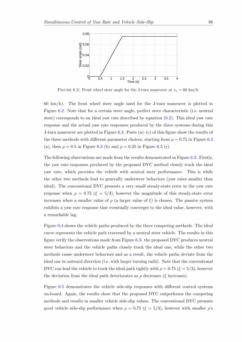
Simultaneous Control of Yaw Rate and Vehicle Side-Slip 98
0 0.5 1 1.5 2 2.5 3 3.5 40
0.02
0.04
0.06
0.08
Time (s)St
eer a
ngle
(rad
)
Figure 6.2: Front wheel steer angle for the J-turn maneuver at vx = 60 km/h.
60 km/h). The front wheel steer angle used for the J-turn maneuver is plotted in
Figure 6.2. Note that for a certain steer angle, perfect steer characteristic (i.e. neutral
steer) corresponds to an ideal yaw rate described by equation (6.2). This ideal yaw rate
response and the actual yaw rate responses produced by the three systems during this
J-turn maneuver are plotted in Figure 6.3. Parts (a)–(c) of this figure show the results of
the three methods with different parameter choices, starting from ρ = 0.75 in Figure 6.3
(a), then ρ = 0.5 in Figure 6.3 (b) and ρ = 0.25 in Figure 6.3 (c).
The following observations are made from the results demonstrated in Figure 6.3. Firstly,
the yaw rate responses produced by the proposed DYC method closely track the ideal
yaw rate, which provides the vehicle with neutral steer performance. This is while
the other two methods lead to generally understeer behaviors (yaw rates smaller than
ideal). The conventional DYC presents a very small steady-state error in the yaw rate
response when ρ = 0.75 (ξ = 5/3), however the magnitude of this steady-state error
increases when a smaller value of ρ (a larger value of ξ) is chosen. The passive system
exhibits a yaw rate response that eventually converges to the ideal value, however, with
a remarkable lag.
Figure 6.4 shows the vehicle paths produced by the three competing methods. The ideal
curve represents the vehicle path traversed by a neutral steer vehicle. The results in this
figure verify the observations made from Figure 6.3: the proposed DYC produces neutral
steer behaviors and the vehicle paths closely track the ideal one, while the other two
methods cause understeer behaviors and as a result, the vehicle paths deviate from the
ideal one in outward direction (i.e. with larger turning radii). Note that the conventional
DYC can lead the vehicle to track the ideal path tightly with ρ = 0.75 (ξ = 5/3), however
the deviation from the ideal path deteriorates as ρ decreases (ξ increases).
Figure 6.5 demonstrates the vehicle side-slip responses with different control systems
on-board. Again, the results show that the proposed DYC outperforms the competing
methods and results in smaller vehicle side-slip values. The conventional DYC presents
good vehicle side-slip performance when ρ = 0.75 (ξ = 5/3), however with smaller ρ’s
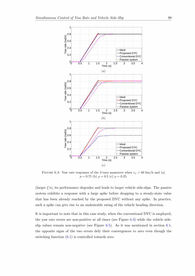
Simultaneous Control of Yaw Rate and Vehicle Side-Slip 99
0 0.5 1 1.5 2 2.5 3 3.5 40
0.2
0.4
0.6
0.8
1
Time (s)Ya
w ra
te (r
ad/s
)
IdealProposed DYCConventional DYCPassive system
(a)
0 0.5 1 1.5 2 2.5 3 3.5 40
0.2
0.4
0.6
0.8
1
Time (s)
Yaw
rate
(rad
/s)
IdealProposed DYCConventional DYCPassive system
(b)
0 0.5 1 1.5 2 2.5 3 3.5 40
0.2
0.4
0.6
0.8
1
Time (s)
Yaw
rate
(rad
/s)
IdealProposed DYCConventional DYCPassive system
(c)
Figure 6.3: Yaw rate responses of the J-turn maneuver when vx = 60 km/h and (a)ρ = 0.75 (b) ρ = 0.5 (c) ρ = 0.25.
(larger ξ’s), its performance degrades and leads to larger vehicle side-slips. The passive
system exhibits a response with a large spike before dropping to a steady-state value
that has been already reached by the proposed DYC without any spike. In practice,
such a spike can give rise to an undesirable swing of the vehicle heading direction.
It is important to note that in this case study, when the conventional DYC is employed,
the yaw rate errors are non-positive at all times (see Figure 6.3) while the vehicle side-
slip values remain non-negative (see Figure 6.5). As it was mentioned in section 6.1,
the opposite signs of the two errors defy their convergences to zero even though the
switching function (6.1) is controlled towards zero.
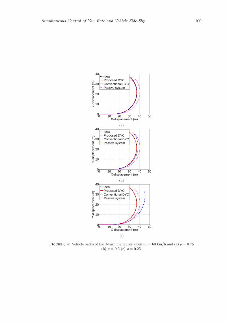
Simultaneous Control of Yaw Rate and Vehicle Side-Slip 100
0 10 20 30 40 500
10
20
30
40
X-displacement (m)
Y-di
spla
cem
ent (
m)
IdealProposed DYCConventional DYCPassive system
(a)
0 10 20 30 40 500
10
20
30
40
X-displacement (m)
Y-di
spla
cem
ent (
m)
IdealProposed DYCConventional DYCPassive system
(b)
0 10 20 30 40 500
10
20
30
40
X-displacement (m)
Y-di
spla
cem
ent (
m)
IdealProposed DYCConventional DYCPassive system
(c)
Figure 6.4: Vehicle paths of the J-turn maneuver when vx = 60 km/h and (a) ρ = 0.75(b) ρ = 0.5 (c) ρ = 0.25.
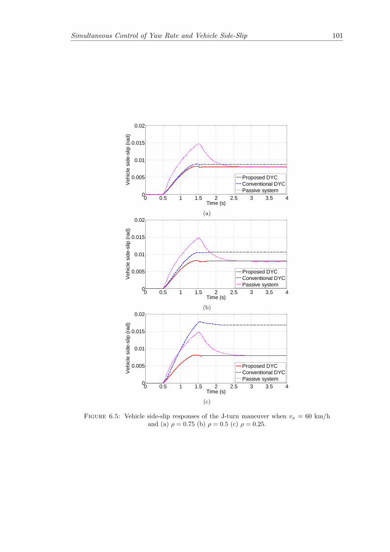
Simultaneous Control of Yaw Rate and Vehicle Side-Slip 101
0 0.5 1 1.5 2 2.5 3 3.5 40
0.005
0.01
0.015
0.02
Time (s)
Vehi
cle
side
-slip
(rad
)
Proposed DYCConventional DYCPassive system
(a)
0 0.5 1 1.5 2 2.5 3 3.5 40
0.005
0.01
0.015
0.02
Time (s)
Vehi
cle
side
-slip
(rad
)
Proposed DYCConventional DYCPassive system
(b)
0 0.5 1 1.5 2 2.5 3 3.5 40
0.005
0.01
0.015
0.02
Time (s)
Vehi
cle
side
-slip
(rad
)
Proposed DYCConventional DYCPassive system
(c)
Figure 6.5: Vehicle side-slip responses of the J-turn maneuver when vx = 60 km/hand (a) ρ = 0.75 (b) ρ = 0.5 (c) ρ = 0.25.
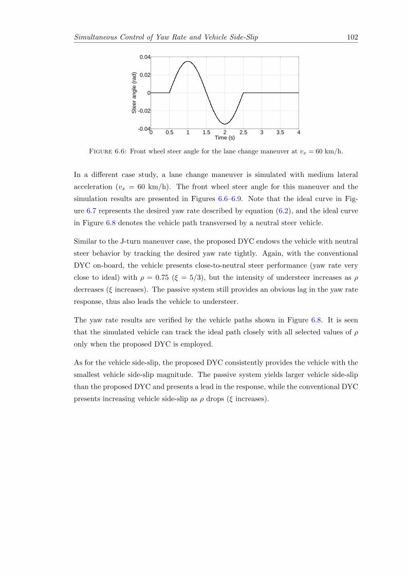
Simultaneous Control of Yaw Rate and Vehicle Side-Slip 102
0 0.5 1 1.5 2 2.5 3 3.5 4-0.04
-0.02
0
0.02
0.04
Time (s)St
eer a
ngle
(rad
)
Figure 6.6: Front wheel steer angle for the lane change maneuver at vx = 60 km/h.
In a different case study, a lane change maneuver is simulated with medium lateral
acceleration (vx = 60 km/h). The front wheel steer angle for this maneuver and the
simulation results are presented in Figures 6.6–6.9. Note that the ideal curve in Fig-
ure 6.7 represents the desired yaw rate described by equation (6.2), and the ideal curve
in Figure 6.8 denotes the vehicle path transversed by a neutral steer vehicle.
Similar to the J-turn maneuver case, the proposed DYC endows the vehicle with neutral
steer behavior by tracking the desired yaw rate tightly. Again, with the conventional
DYC on-board, the vehicle presents close-to-neutral steer performance (yaw rate very
close to ideal) with ρ = 0.75 (ξ = 5/3), but the intensity of understeer increases as ρ
decreases (ξ increases). The passive system still provides an obvious lag in the yaw rate
response, thus also leads the vehicle to understeer.
The yaw rate results are verified by the vehicle paths shown in Figure 6.8. It is seen
that the simulated vehicle can track the ideal path closely with all selected values of ρ
only when the proposed DYC is employed.
As for the vehicle side-slip, the proposed DYC consistently provides the vehicle with the
smallest vehicle side-slip magnitude. The passive system yields larger vehicle side-slip
than the proposed DYC and presents a lead in the response, while the conventional DYC
presents increasing vehicle side-slip as ρ drops (ξ increases).
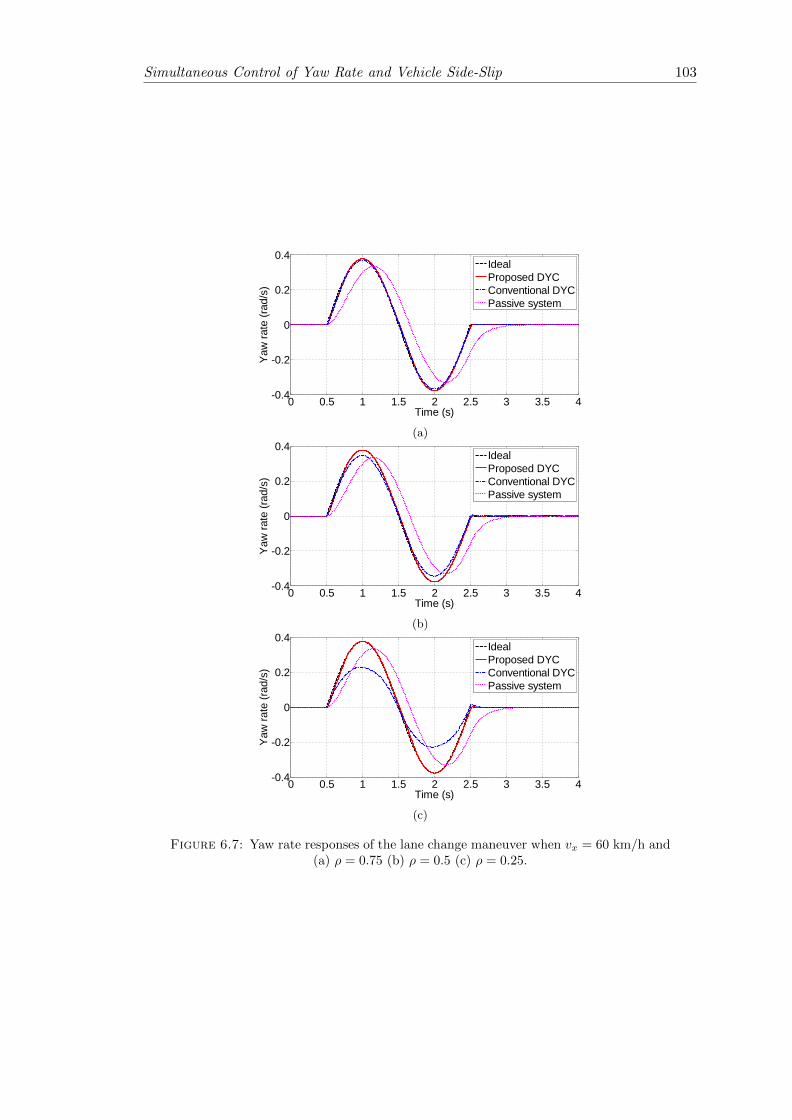
Simultaneous Control of Yaw Rate and Vehicle Side-Slip 103
0 0.5 1 1.5 2 2.5 3 3.5 4-0.4
-0.2
0
0.2
0.4
Time (s)
Yaw
rate
(rad
/s)
IdealProposed DYCConventional DYCPassive system
(a)
0 0.5 1 1.5 2 2.5 3 3.5 4-0.4
-0.2
0
0.2
0.4
Time (s)
Yaw
rate
(rad
/s)
IdealProposed DYCConventional DYCPassive system
(b)
0 0.5 1 1.5 2 2.5 3 3.5 4-0.4
-0.2
0
0.2
0.4
Time (s)
Yaw
rate
(rad
/s)
IdealProposed DYCConventional DYCPassive system
(c)
Figure 6.7: Yaw rate responses of the lane change maneuver when vx = 60 km/h and(a) ρ = 0.75 (b) ρ = 0.5 (c) ρ = 0.25.
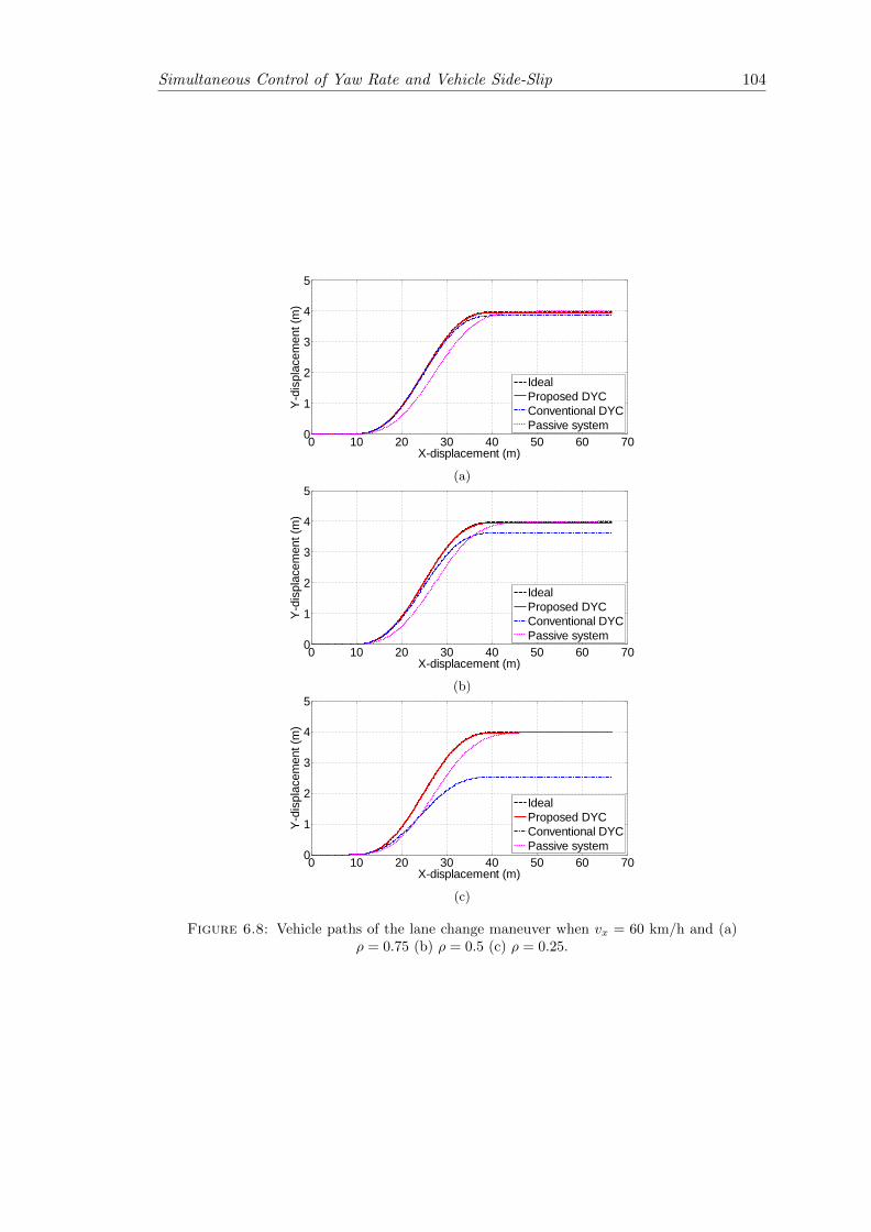
Simultaneous Control of Yaw Rate and Vehicle Side-Slip 104
0 10 20 30 40 50 60 700
1
2
3
4
5
X-displacement (m)
Y-di
spla
cem
ent (
m)
IdealProposed DYCConventional DYCPassive system
(a)
0 10 20 30 40 50 60 700
1
2
3
4
5
X-displacement (m)
Y-di
spla
cem
ent (
m)
IdealProposed DYCConventional DYCPassive system
(b)
0 10 20 30 40 50 60 700
1
2
3
4
5
X-displacement (m)
Y-di
spla
cem
ent (
m)
IdealProposed DYCConventional DYCPassive system
(c)
Figure 6.8: Vehicle paths of the lane change maneuver when vx = 60 km/h and (a)ρ = 0.75 (b) ρ = 0.5 (c) ρ = 0.25.
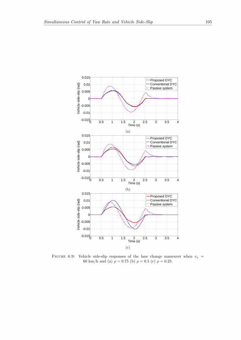
Simultaneous Control of Yaw Rate and Vehicle Side-Slip 105
0 0.5 1 1.5 2 2.5 3 3.5 4-0.015
-0.01
-0.005
0
0.005
0.01
0.015
Time (s)
Vehi
cle
side
-slip
(rad
)
Proposed DYCConventional DYCPassive system
(a)
0 0.5 1 1.5 2 2.5 3 3.5 4-0.015
-0.01
-0.005
0
0.005
0.01
0.015
Time (s)
Vehi
cle
side
-slip
(rad
)
Proposed DYCConventional DYCPassive system
(b)
0 0.5 1 1.5 2 2.5 3 3.5 4-0.015
-0.01
-0.005
0
0.005
0.01
0.015
Time (s)
Vehi
cle
side
-slip
(rad
)
Proposed DYCConventional DYCPassive system
(c)
Figure 6.9: Vehicle side-slip responses of the lane change maneuver when vx =60 km/h and (a) ρ = 0.75 (b) ρ = 0.5 (c) ρ = 0.25.
Simultaneous Control of Yaw Rate and Vehicle Side-Slip 106
6.3.1.2 J-turn and lane change maneuvers at vx = 80 km/h
This section presents the results of the simulated J-turn and lane change maneuvers in
presence of high lateral acceleration caused by high longitudinal velocity (vx = 80 km/h).
Figure 6.10 shows the steering input used to simulate the J-turn maneuver. The yaw
rate responses, vehicle paths and vehicle side-slip responses during this J-turn maneuver
are presented in Figures 6.11, 6.12 and 6.13, respectively. It is observed that in this
high speed maneuver, the proposed DYC still leads the vehicle to track the desired yaw
rate closely, and in turn makes the vehicle traverse in a path very close to the ideal one.
Meanwhile, the passive system causes an obvious lag in the yaw rate response, deviating
the vehicle path outward. The conventional DYC produces oversteer performance (yaw
rate larger than ideal) and bends the vehicle path inward, which behavior deteriorates
with smaller ρ values (larger ξ values).
In terms of the vehicle side-slip, it can be seen in Figure 6.13 that with the conventional
DYC on-board, the vehicle side-slip remains small when ρ is large (ξ is small), however
it diverges and the vehicle tends to spin as ρ decreases (ξ increase). In addition, the
passive system exhibits a very slow oscillation: the vehicle side-slip climbs up slowly and
then drops sluggishly. This slow convergence and the change of sign in vehicle side-slip
do harm to the driver’s sense of control. The proposed DYC produces fast convergence
and small vehicle side-slip magnitude for all ρ values.
The steering command and vehicle responses for the lane change maneuver with high
lateral acceleration (vx = 80 km/h) are shown in Figures 6.14–6.17. The observations
are similar to the case study of J-turn maneuver at high speed: with the proposed
DYC on-board, the vehicle closely follows the ideal path, with its yaw rate tracking the
ideal value tightly and its vehicle side-slip magnitude being generally less than the other
methods. The conventional DYC results in intensifying oversteer behavior as well as
increasing vehicle side-slip, with decreasing ρ (increasing ξ). The passive system causes
a lag in the yaw rate response which gives rise to understeer performance. In the vehicle
side-slip response, the passive system presents a remarkable phase difference from the
other two, with a spike at the end of the steering command (t = 2.5 s).
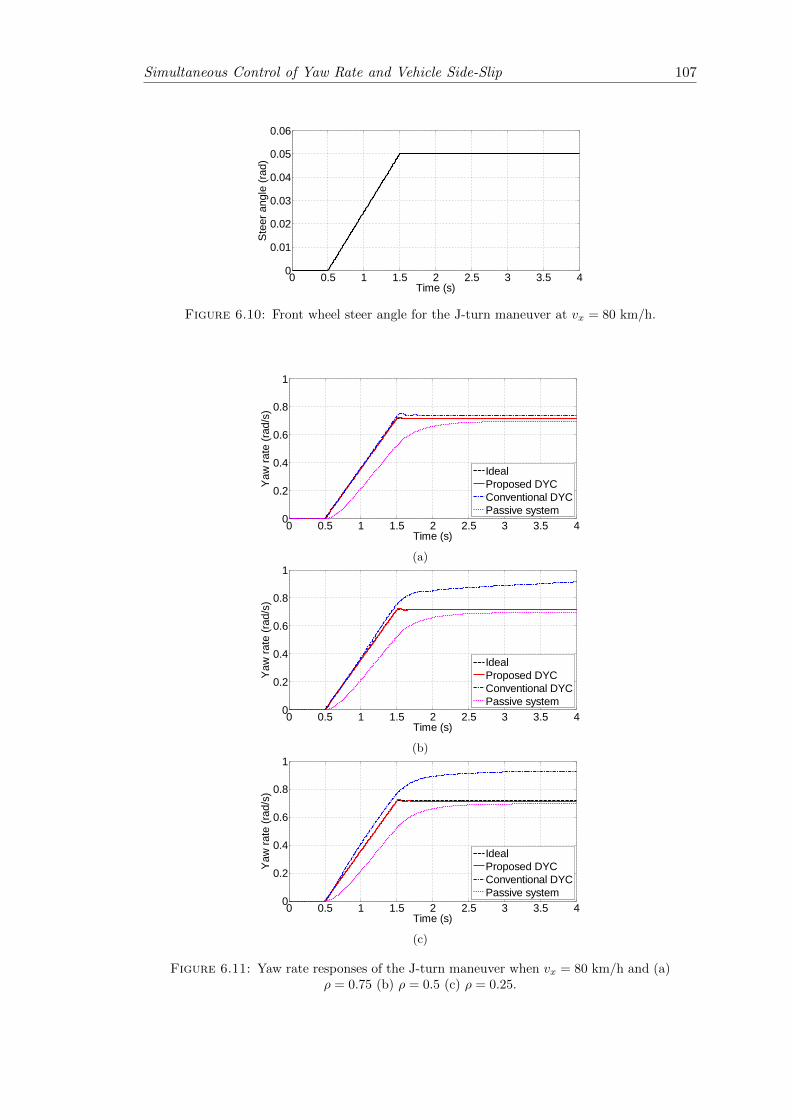
Simultaneous Control of Yaw Rate and Vehicle Side-Slip 107
0 0.5 1 1.5 2 2.5 3 3.5 40
0.01
0.02
0.03
0.04
0.05
0.06
Time (s)
Stee
r ang
le (r
ad)
Figure 6.10: Front wheel steer angle for the J-turn maneuver at vx = 80 km/h.
0 0.5 1 1.5 2 2.5 3 3.5 40
0.2
0.4
0.6
0.8
1
Time (s)
Yaw
rate
(rad
/s)
IdealProposed DYCConventional DYCPassive system
(a)
0 0.5 1 1.5 2 2.5 3 3.5 40
0.2
0.4
0.6
0.8
1
Time (s)
Yaw
rate
(rad
/s)
IdealProposed DYCConventional DYCPassive system
(b)
0 0.5 1 1.5 2 2.5 3 3.5 40
0.2
0.4
0.6
0.8
1
Time (s)
Yaw
rate
(rad
/s)
IdealProposed DYCConventional DYCPassive system
(c)
Figure 6.11: Yaw rate responses of the J-turn maneuver when vx = 80 km/h and (a)ρ = 0.75 (b) ρ = 0.5 (c) ρ = 0.25.
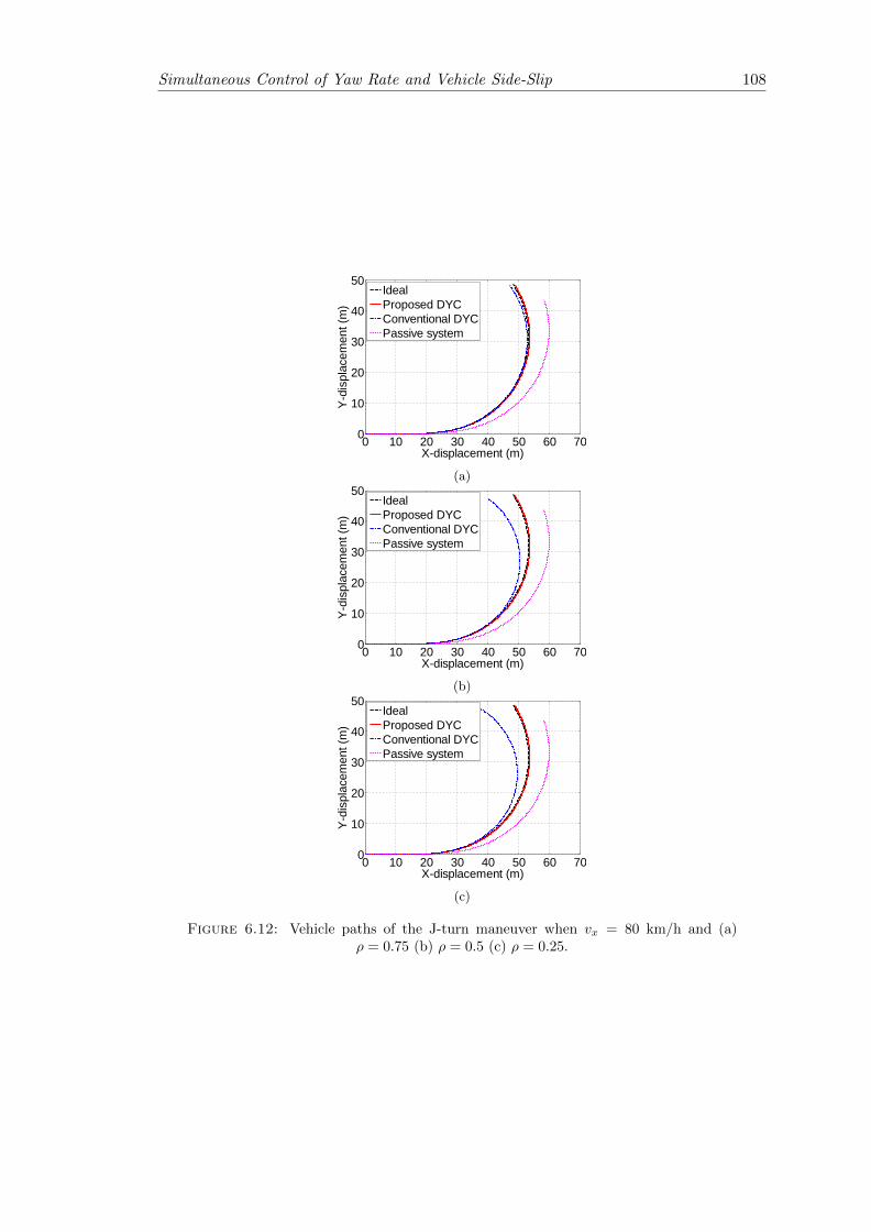
Simultaneous Control of Yaw Rate and Vehicle Side-Slip 108
0 10 20 30 40 50 60 700
10
20
30
40
50
X-displacement (m)
Y-di
spla
cem
ent (
m)
IdealProposed DYCConventional DYCPassive system
(a)
0 10 20 30 40 50 60 700
10
20
30
40
50
X-displacement (m)
Y-di
spla
cem
ent (
m)
IdealProposed DYCConventional DYCPassive system
(b)
0 10 20 30 40 50 60 700
10
20
30
40
50
X-displacement (m)
Y-di
spla
cem
ent (
m)
IdealProposed DYCConventional DYCPassive system
(c)
Figure 6.12: Vehicle paths of the J-turn maneuver when vx = 80 km/h and (a)ρ = 0.75 (b) ρ = 0.5 (c) ρ = 0.25.
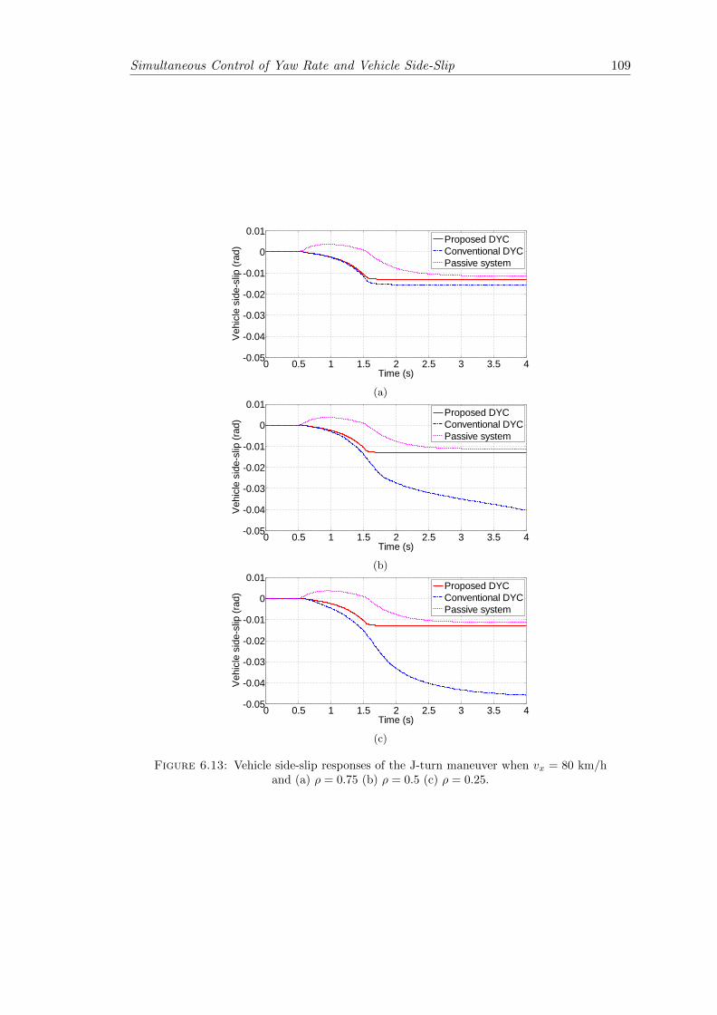
Simultaneous Control of Yaw Rate and Vehicle Side-Slip 109
0 0.5 1 1.5 2 2.5 3 3.5 4-0.05
-0.04
-0.03
-0.02
-0.01
0
0.01
Time (s)
Vehi
cle
side
-slip
(rad
)
Proposed DYCConventional DYCPassive system
(a)
0 0.5 1 1.5 2 2.5 3 3.5 4-0.05
-0.04
-0.03
-0.02
-0.01
0
0.01
Time (s)
Vehi
cle
side
-slip
(rad
)
Proposed DYCConventional DYCPassive system
(b)
0 0.5 1 1.5 2 2.5 3 3.5 4-0.05
-0.04
-0.03
-0.02
-0.01
0
0.01
Time (s)
Vehi
cle
side
-slip
(rad
)
Proposed DYCConventional DYCPassive system
(c)
Figure 6.13: Vehicle side-slip responses of the J-turn maneuver when vx = 80 km/hand (a) ρ = 0.75 (b) ρ = 0.5 (c) ρ = 0.25.
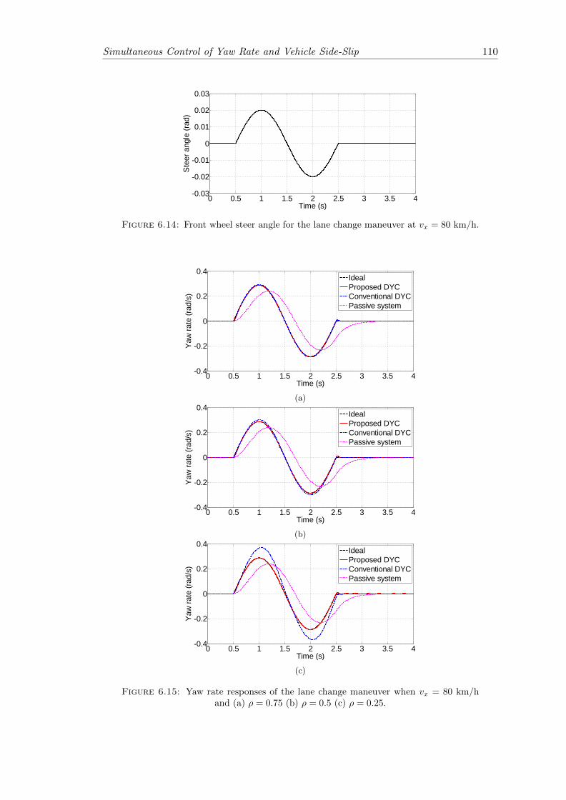
Simultaneous Control of Yaw Rate and Vehicle Side-Slip 110
0 0.5 1 1.5 2 2.5 3 3.5 4-0.03
-0.02
-0.01
0
0.01
0.02
0.03
Time (s)
Stee
r ang
le (r
ad)
Figure 6.14: Front wheel steer angle for the lane change maneuver at vx = 80 km/h.
0 0.5 1 1.5 2 2.5 3 3.5 4-0.4
-0.2
0
0.2
0.4
Time (s)
Yaw
rate
(rad
/s)
IdealProposed DYCConventional DYCPassive system
(a)
0 0.5 1 1.5 2 2.5 3 3.5 4-0.4
-0.2
0
0.2
0.4
Time (s)
Yaw
rate
(rad
/s)
IdealProposed DYCConventional DYCPassive system
(b)
0 0.5 1 1.5 2 2.5 3 3.5 4-0.4
-0.2
0
0.2
0.4
Time (s)
Yaw
rate
(rad
/s)
IdealProposed DYCConventional DYCPassive system
(c)
Figure 6.15: Yaw rate responses of the lane change maneuver when vx = 80 km/hand (a) ρ = 0.75 (b) ρ = 0.5 (c) ρ = 0.25.
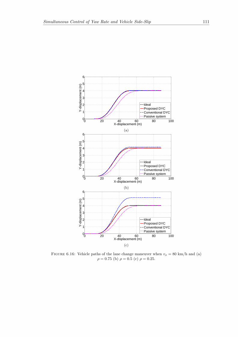
Simultaneous Control of Yaw Rate and Vehicle Side-Slip 111
0 20 40 60 80 1000
1
2
3
4
5
6
X-displacement (m)
Y-di
spla
cem
ent (
m)
IdealProposed DYCConventional DYCPassive system
(a)
0 20 40 60 80 1000
1
2
3
4
5
6
X-displacement (m)
Y-di
spla
cem
ent (
m)
IdealProposed DYCConventional DYCPassive system
(b)
0 20 40 60 80 1000
1
2
3
4
5
6
X-displacement (m)
Y-di
spla
cem
ent (
m)
IdealProposed DYCConventional DYCPassive system
(c)
Figure 6.16: Vehicle paths of the lane change maneuver when vx = 80 km/h and (a)ρ = 0.75 (b) ρ = 0.5 (c) ρ = 0.25.
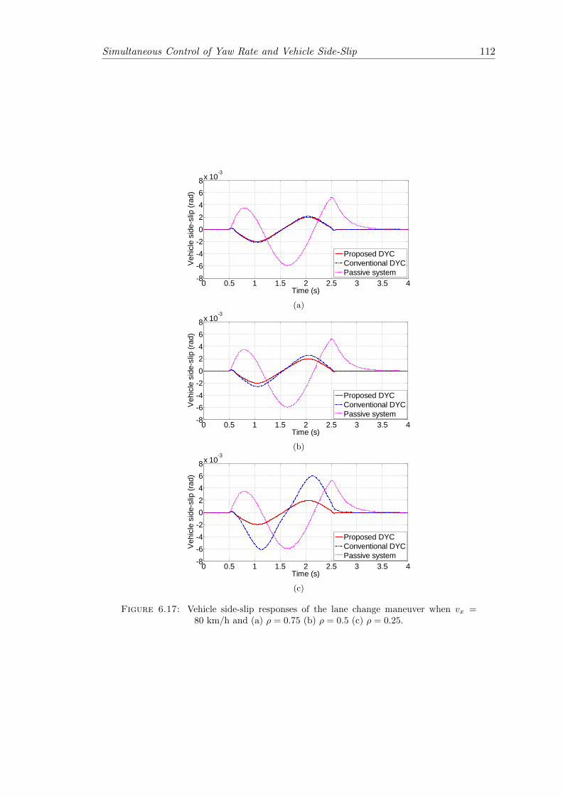
Simultaneous Control of Yaw Rate and Vehicle Side-Slip 112
0 0.5 1 1.5 2 2.5 3 3.5 4-8-6-4-202468x 10
-3
Time (s)
Vehi
cle
side
-slip
(rad
)
Proposed DYCConventional DYCPassive system
(a)
0 0.5 1 1.5 2 2.5 3 3.5 4-8-6-4-202468x 10
-3
Time (s)
Vehi
cle
side
-slip
(rad
)
Proposed DYCConventional DYCPassive system
(b)
0 0.5 1 1.5 2 2.5 3 3.5 4-8-6-4-202468x 10
-3
Time (s)
Vehi
cle
side
-slip
(rad
)
Proposed DYCConventional DYCPassive system
(c)
Figure 6.17: Vehicle side-slip responses of the lane change maneuver when vx =80 km/h and (a) ρ = 0.75 (b) ρ = 0.5 (c) ρ = 0.25.
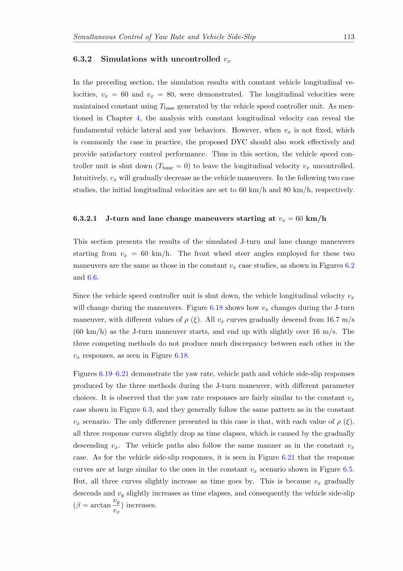
Simultaneous Control of Yaw Rate and Vehicle Side-Slip 113
6.3.2 Simulations with uncontrolled vx
In the preceding section, the simulation results with constant vehicle longitudinal ve-
locities, vx = 60 and vx = 80, were demonstrated. The longitudinal velocities were
maintained constant using Tbase generated by the vehicle speed controller unit. As men-
tioned in Chapter 4, the analysis with constant longitudinal velocity can reveal the
fundamental vehicle lateral and yaw behaviors. However, when vx is not fixed, which
is commonly the case in practice, the proposed DYC should also work effectively and
provide satisfactory control performance. Thus in this section, the vehicle speed con-
troller unit is shut down (Tbase = 0) to leave the longitudinal velocity vx uncontrolled.
Intuitively, vx will gradually decrease as the vehicle maneuvers. In the following two case
studies, the initial longitudinal velocities are set to 60 km/h and 80 km/h, respectively.
6.3.2.1 J-turn and lane change maneuvers starting at vx = 60 km/h
This section presents the results of the simulated J-turn and lane change maneuvers
starting from vx = 60 km/h. The front wheel steer angles employed for these two
maneuvers are the same as those in the constant vx case studies, as shown in Figures 6.2
and 6.6.
Since the vehicle speed controller unit is shut down, the vehicle longitudinal velocity vx
will change during the maneuvers. Figure 6.18 shows how vx changes during the J-turn
maneuver, with different values of ρ (ξ). All vx curves gradually descend from 16.7 m/s
(60 km/h) as the J-turn maneuver starts, and end up with slightly over 16 m/s. The
three competing methods do not produce much discrepancy between each other in the
vx responses, as seen in Figure 6.18.
Figures 6.19–6.21 demonstrate the yaw rate, vehicle path and vehicle side-slip responses
produced by the three methods during the J-turn maneuver, with different parameter
choices. It is observed that the yaw rate responses are fairly similar to the constant vx
case shown in Figure 6.3, and they generally follow the same pattern as in the constant
vx scenario. The only difference presented in this case is that, with each value of ρ (ξ),
all three response curves slightly drop as time elapses, which is caused by the gradually
descending vx. The vehicle paths also follow the same manner as in the constant vx
case. As for the vehicle side-slip responses, it is seen in Figure 6.21 that the response
curves are at large similar to the ones in the constant vx scenario shown in Figure 6.5.
But, all three curves slightly increase as time goes by. This is because vx gradually
descends and vy slightly increases as time elapses, and consequently the vehicle side-slip
(β = arctanvyvx
) increases.
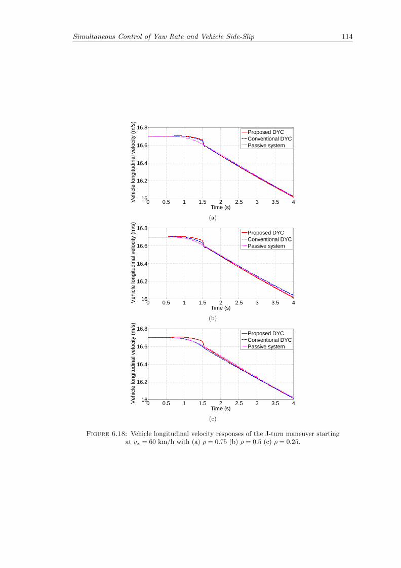
Simultaneous Control of Yaw Rate and Vehicle Side-Slip 114
0 0.5 1 1.5 2 2.5 3 3.5 416
16.2
16.4
16.6
16.8
Time (s)
Vehi
cle
long
itudi
nal v
eloc
ity (m
/s)
Proposed DYCConventional DYCPassive system
(a)
0 0.5 1 1.5 2 2.5 3 3.5 416
16.2
16.4
16.6
16.8
Time (s)
Vehi
cle
long
itudi
nal v
eloc
ity (m
/s)
Proposed DYCConventional DYCPassive system
(b)
0 0.5 1 1.5 2 2.5 3 3.5 416
16.2
16.4
16.6
16.8
Time (s)
Vehi
cle
long
itudi
nal v
eloc
ity (m
/s)
Proposed DYCConventional DYCPassive system
(c)
Figure 6.18: Vehicle longitudinal velocity responses of the J-turn maneuver startingat vx = 60 km/h with (a) ρ = 0.75 (b) ρ = 0.5 (c) ρ = 0.25.
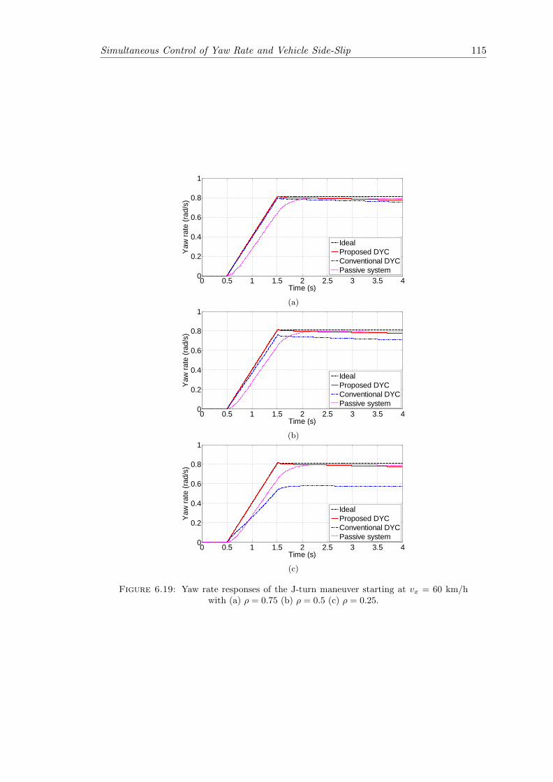
Simultaneous Control of Yaw Rate and Vehicle Side-Slip 115
0 0.5 1 1.5 2 2.5 3 3.5 40
0.2
0.4
0.6
0.8
1
Time (s)
Yaw
rate
(rad
/s)
IdealProposed DYCConventional DYCPassive system
(a)
0 0.5 1 1.5 2 2.5 3 3.5 40
0.2
0.4
0.6
0.8
1
Time (s)
Yaw
rate
(rad
/s)
IdealProposed DYCConventional DYCPassive system
(b)
0 0.5 1 1.5 2 2.5 3 3.5 40
0.2
0.4
0.6
0.8
1
Time (s)
Yaw
rate
(rad
/s)
IdealProposed DYCConventional DYCPassive system
(c)
Figure 6.19: Yaw rate responses of the J-turn maneuver starting at vx = 60 km/hwith (a) ρ = 0.75 (b) ρ = 0.5 (c) ρ = 0.25.
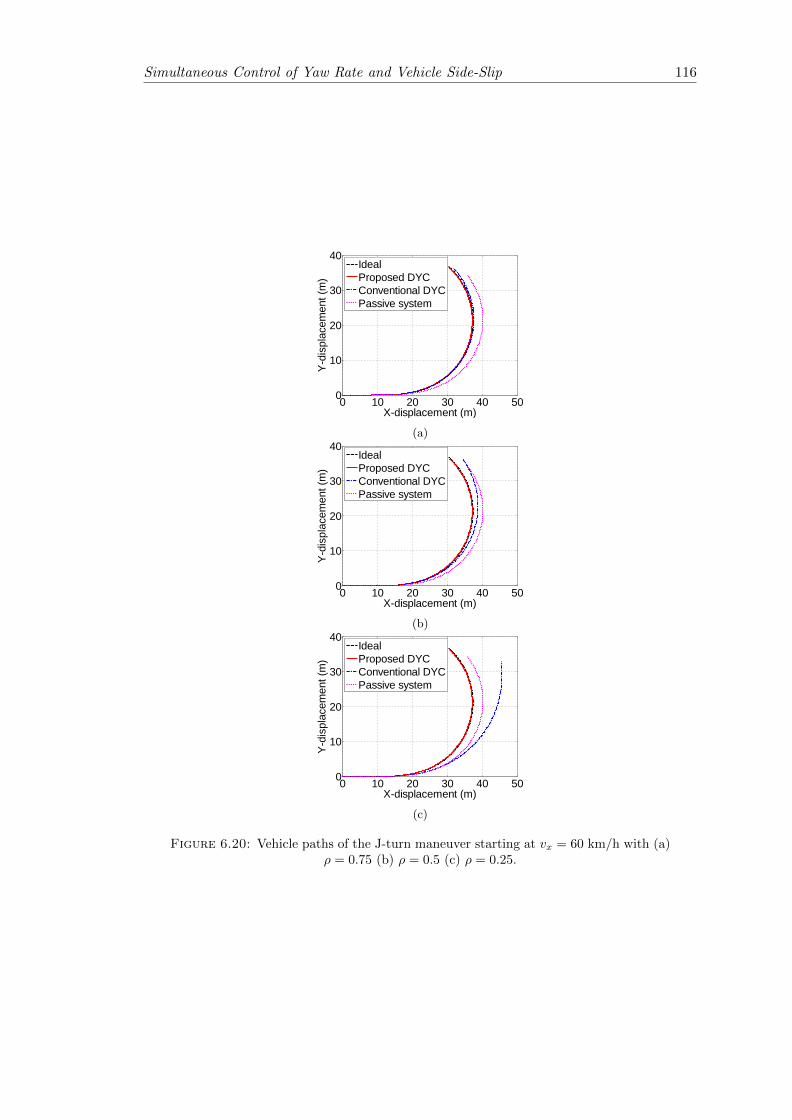
Simultaneous Control of Yaw Rate and Vehicle Side-Slip 116
0 10 20 30 40 500
10
20
30
40
X-displacement (m)
Y-di
spla
cem
ent (
m)
IdealProposed DYCConventional DYCPassive system
(a)
0 10 20 30 40 500
10
20
30
40
X-displacement (m)
Y-di
spla
cem
ent (
m)
IdealProposed DYCConventional DYCPassive system
(b)
0 10 20 30 40 500
10
20
30
40
X-displacement (m)
Y-di
spla
cem
ent (
m)
IdealProposed DYCConventional DYCPassive system
(c)
Figure 6.20: Vehicle paths of the J-turn maneuver starting at vx = 60 km/h with (a)ρ = 0.75 (b) ρ = 0.5 (c) ρ = 0.25.
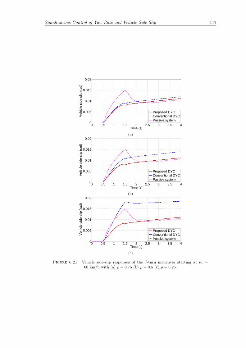
Simultaneous Control of Yaw Rate and Vehicle Side-Slip 117
0 0.5 1 1.5 2 2.5 3 3.5 40
0.005
0.01
0.015
0.02
Time (s)
Vehi
cle
side
-slip
(rad
)
Proposed DYCConventional DYCPassive system
(a)
0 0.5 1 1.5 2 2.5 3 3.5 40
0.005
0.01
0.015
0.02
Time (s)
Vehi
cle
side
-slip
(rad
)
Proposed DYCConventional DYCPassive system
(b)
0 0.5 1 1.5 2 2.5 3 3.5 40
0.005
0.01
0.015
0.02
Time (s)
Vehi
cle
side
-slip
(rad
)
Proposed DYCConventional DYCPassive system
(c)
Figure 6.21: Vehicle side-slip responses of the J-turn maneuver starting at vx =60 km/h with (a) ρ = 0.75 (b) ρ = 0.5 (c) ρ = 0.25.
Simultaneous Control of Yaw Rate and Vehicle Side-Slip 118
Figure 6.22 shows how vx changes during the lane change maneuver, starting from vx =
60 km/h with different values of ρ (ξ). During this maneuver, with each value of ρ (ξ),
the three response curves present slight decreases with some oscillations. The proposed
DYC generally produces the largest oscillation, but this does not impair the vehicle
performance as the magnitude of this oscillation is very small. With the conventional
DYC on-board, the vx oscillation gradually abates as ρ drops (ξ increases). The passive
system, on the other hand, produces the smoothest vx response.
Figures 6.23–6.25 demonstrate the yaw rate, vehicle path and vehicle side-slip responses
during the lane change maneuver, employing different parameter choices. It can be seen
that these three types of vehicle responses are almost the same as the responses in the
constant vx case presented in Figures 6.7–6.9. This similarity is easily comprehensible:
even though vx in general drops with all three methods on-board, yet the magnitudes
of the vx variations are quite small.
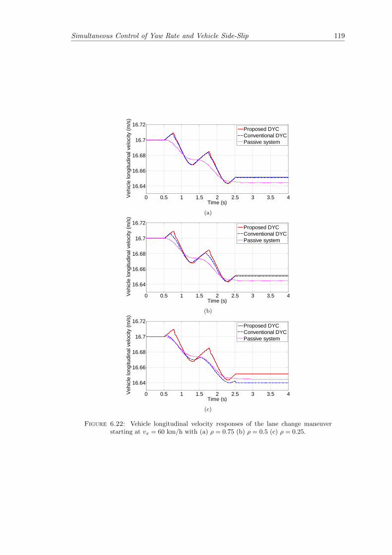
Simultaneous Control of Yaw Rate and Vehicle Side-Slip 119
0 0.5 1 1.5 2 2.5 3 3.5 4
16.64
16.66
16.68
16.7
16.72
Time (s)
Vehi
cle
long
itudi
nal v
eloc
ity (m
/s)
Proposed DYCConventional DYCPassive system
(a)
0 0.5 1 1.5 2 2.5 3 3.5 4
16.64
16.66
16.68
16.7
16.72
Time (s)
Vehi
cle
long
itudi
nal v
eloc
ity (m
/s)
Proposed DYCConventional DYCPassive system
(b)
0 0.5 1 1.5 2 2.5 3 3.5 4
16.64
16.66
16.68
16.7
16.72
Time (s)
Vehi
cle
long
itudi
nal v
eloc
ity (m
/s)
Proposed DYCConventional DYCPassive system
(c)
Figure 6.22: Vehicle longitudinal velocity responses of the lane change maneuverstarting at vx = 60 km/h with (a) ρ = 0.75 (b) ρ = 0.5 (c) ρ = 0.25.
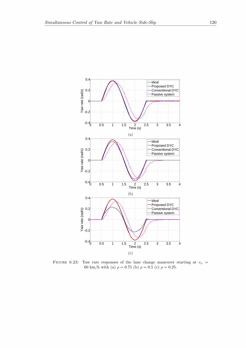
Simultaneous Control of Yaw Rate and Vehicle Side-Slip 120
0 0.5 1 1.5 2 2.5 3 3.5 4-0.4
-0.2
0
0.2
0.4
Time (s)
Yaw
rate
(rad
/s)
IdealProposed DYCConventional DYCPassive system
(a)
0 0.5 1 1.5 2 2.5 3 3.5 4-0.4
-0.2
0
0.2
0.4
Time (s)
Yaw
rate
(rad
/s)
IdealProposed DYCConventional DYCPassive system
(b)
0 0.5 1 1.5 2 2.5 3 3.5 4-0.4
-0.2
0
0.2
0.4
Time (s)
Yaw
rate
(rad
/s)
IdealProposed DYCConventional DYCPassive system
(c)
Figure 6.23: Yaw rate responses of the lane change maneuver starting at vx =60 km/h with (a) ρ = 0.75 (b) ρ = 0.5 (c) ρ = 0.25.
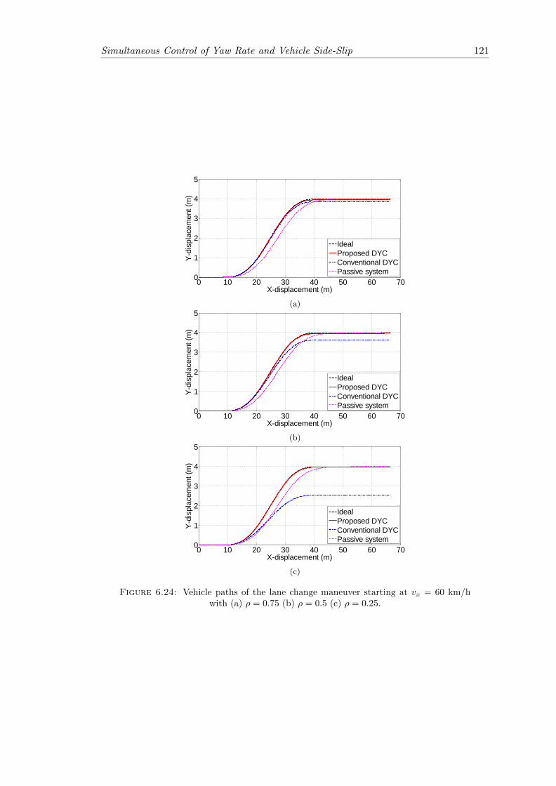
Simultaneous Control of Yaw Rate and Vehicle Side-Slip 121
0 10 20 30 40 50 60 700
1
2
3
4
5
X-displacement (m)
Y-di
spla
cem
ent (
m)
IdealProposed DYCConventional DYCPassive system
(a)
0 10 20 30 40 50 60 700
1
2
3
4
5
X-displacement (m)
Y-di
spla
cem
ent (
m)
IdealProposed DYCConventional DYCPassive system
(b)
0 10 20 30 40 50 60 700
1
2
3
4
5
X-displacement (m)
Y-di
spla
cem
ent (
m)
IdealProposed DYCConventional DYCPassive system
(c)
Figure 6.24: Vehicle paths of the lane change maneuver starting at vx = 60 km/hwith (a) ρ = 0.75 (b) ρ = 0.5 (c) ρ = 0.25.
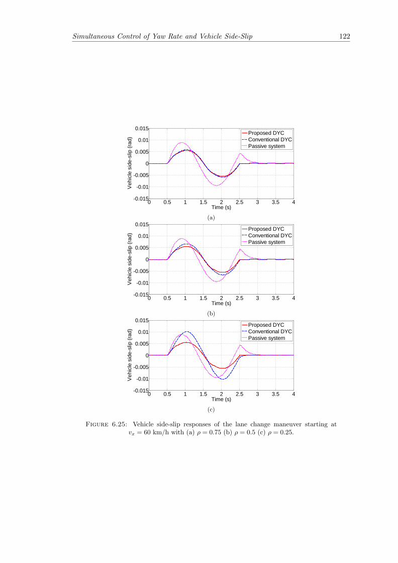
Simultaneous Control of Yaw Rate and Vehicle Side-Slip 122
0 0.5 1 1.5 2 2.5 3 3.5 4-0.015
-0.01
-0.005
0
0.005
0.01
0.015
Time (s)
Vehi
cle
side
-slip
(rad
)
Proposed DYCConventional DYCPassive system
(a)
0 0.5 1 1.5 2 2.5 3 3.5 4-0.015
-0.01
-0.005
0
0.005
0.01
0.015
Time (s)
Vehi
cle
side
-slip
(rad
)
Proposed DYCConventional DYCPassive system
(b)
0 0.5 1 1.5 2 2.5 3 3.5 4-0.015
-0.01
-0.005
0
0.005
0.01
0.015
Time (s)
Vehi
cle
side
-slip
(rad
)
Proposed DYCConventional DYCPassive system
(c)
Figure 6.25: Vehicle side-slip responses of the lane change maneuver starting atvx = 60 km/h with (a) ρ = 0.75 (b) ρ = 0.5 (c) ρ = 0.25.
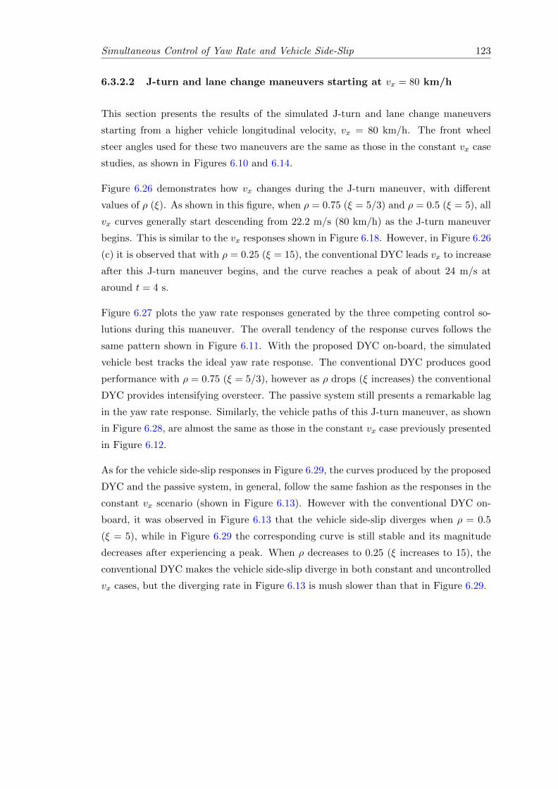
Simultaneous Control of Yaw Rate and Vehicle Side-Slip 123
6.3.2.2 J-turn and lane change maneuvers starting at vx = 80 km/h
This section presents the results of the simulated J-turn and lane change maneuvers
starting from a higher vehicle longitudinal velocity, vx = 80 km/h. The front wheel
steer angles used for these two maneuvers are the same as those in the constant vx case
studies, as shown in Figures 6.10 and 6.14.
Figure 6.26 demonstrates how vx changes during the J-turn maneuver, with different
values of ρ (ξ). As shown in this figure, when ρ = 0.75 (ξ = 5/3) and ρ = 0.5 (ξ = 5), all
vx curves generally start descending from 22.2 m/s (80 km/h) as the J-turn maneuver
begins. This is similar to the vx responses shown in Figure 6.18. However, in Figure 6.26
(c) it is observed that with ρ = 0.25 (ξ = 15), the conventional DYC leads vx to increase
after this J-turn maneuver begins, and the curve reaches a peak of about 24 m/s at
around t = 4 s.
Figure 6.27 plots the yaw rate responses generated by the three competing control so-
lutions during this maneuver. The overall tendency of the response curves follows the
same pattern shown in Figure 6.11. With the proposed DYC on-board, the simulated
vehicle best tracks the ideal yaw rate response. The conventional DYC produces good
performance with ρ = 0.75 (ξ = 5/3), however as ρ drops (ξ increases) the conventional
DYC provides intensifying oversteer. The passive system still presents a remarkable lag
in the yaw rate response. Similarly, the vehicle paths of this J-turn maneuver, as shown
in Figure 6.28, are almost the same as those in the constant vx case previously presented
in Figure 6.12.
As for the vehicle side-slip responses in Figure 6.29, the curves produced by the proposed
DYC and the passive system, in general, follow the same fashion as the responses in the
constant vx scenario (shown in Figure 6.13). However with the conventional DYC on-
board, it was observed in Figure 6.13 that the vehicle side-slip diverges when ρ = 0.5
(ξ = 5), while in Figure 6.29 the corresponding curve is still stable and its magnitude
decreases after experiencing a peak. When ρ decreases to 0.25 (ξ increases to 15), the
conventional DYC makes the vehicle side-slip diverge in both constant and uncontrolled
vx cases, but the diverging rate in Figure 6.13 is mush slower than that in Figure 6.29.
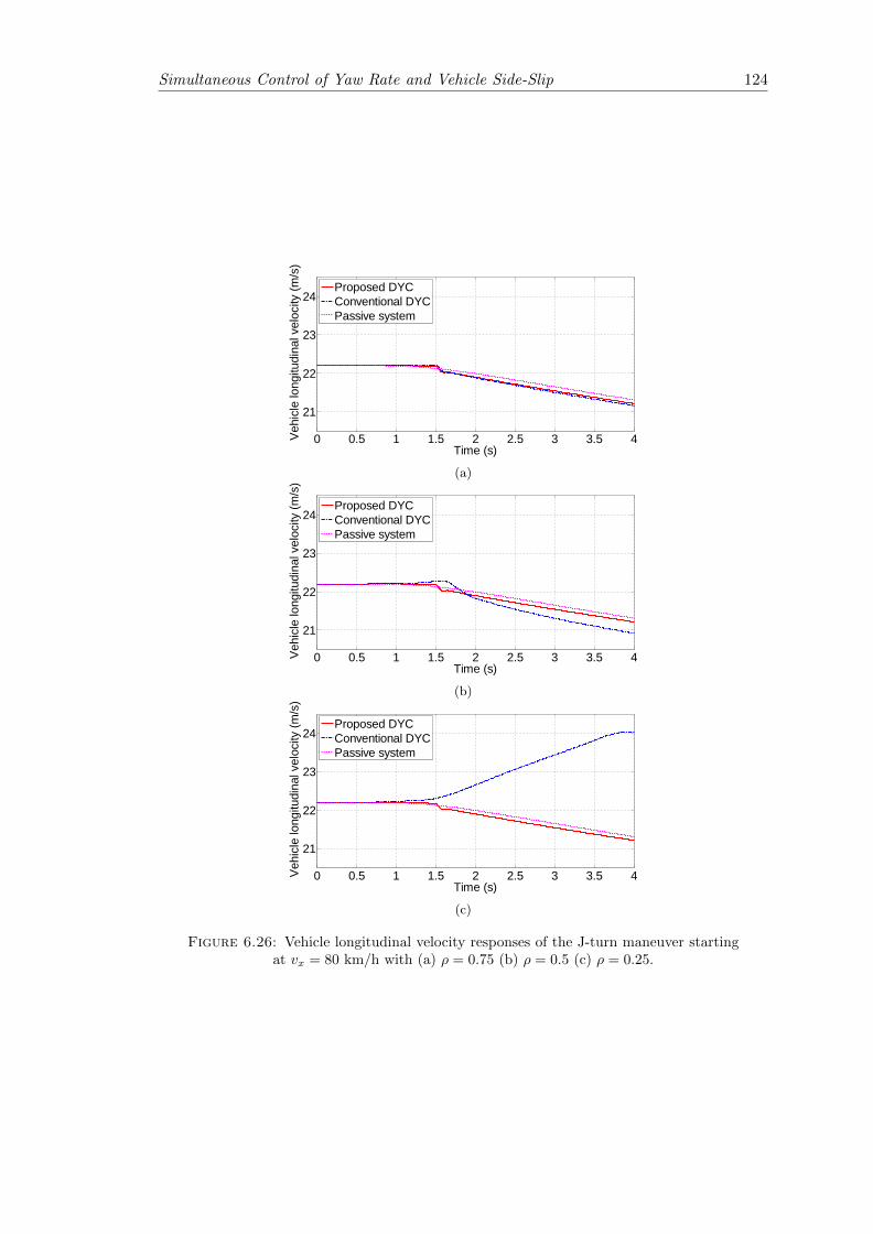
Simultaneous Control of Yaw Rate and Vehicle Side-Slip 124
0 0.5 1 1.5 2 2.5 3 3.5 4
21
22
23
24
Time (s)
Vehi
cle
long
itudi
nal v
eloc
ity (m
/s)
Proposed DYCConventional DYCPassive system
(a)
0 0.5 1 1.5 2 2.5 3 3.5 4
21
22
23
24
Time (s)
Vehi
cle
long
itudi
nal v
eloc
ity (m
/s)
Proposed DYCConventional DYCPassive system
(b)
0 0.5 1 1.5 2 2.5 3 3.5 4
21
22
23
24
Time (s)
Vehi
cle
long
itudi
nal v
eloc
ity (m
/s)
Proposed DYCConventional DYCPassive system
(c)
Figure 6.26: Vehicle longitudinal velocity responses of the J-turn maneuver startingat vx = 80 km/h with (a) ρ = 0.75 (b) ρ = 0.5 (c) ρ = 0.25.
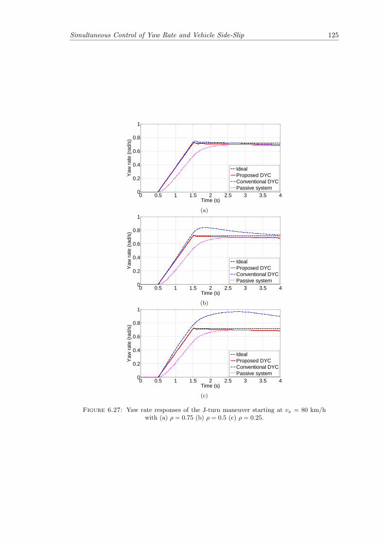
Simultaneous Control of Yaw Rate and Vehicle Side-Slip 125
0 0.5 1 1.5 2 2.5 3 3.5 40
0.2
0.4
0.6
0.8
1
Time (s)
Yaw
rate
(rad
/s)
IdealProposed DYCConventional DYCPassive system
(a)
0 0.5 1 1.5 2 2.5 3 3.5 40
0.2
0.4
0.6
0.8
1
Time (s)
Yaw
rate
(rad
/s)
IdealProposed DYCConventional DYCPassive system
(b)
0 0.5 1 1.5 2 2.5 3 3.5 40
0.2
0.4
0.6
0.8
1
Time (s)
Yaw
rate
(rad
/s)
IdealProposed DYCConventional DYCPassive system
(c)
Figure 6.27: Yaw rate responses of the J-turn maneuver starting at vx = 80 km/hwith (a) ρ = 0.75 (b) ρ = 0.5 (c) ρ = 0.25.
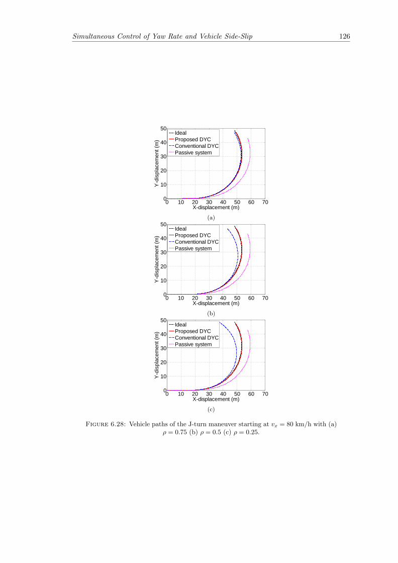
Simultaneous Control of Yaw Rate and Vehicle Side-Slip 126
0 10 20 30 40 50 60 700
10
20
30
40
50
X-displacement (m)
Y-di
spla
cem
ent (
m)
IdealProposed DYCConventional DYCPassive system
(a)
0 10 20 30 40 50 60 700
10
20
30
40
50
X-displacement (m)
Y-di
spla
cem
ent (
m)
IdealProposed DYCConventional DYCPassive system
(b)
0 10 20 30 40 50 60 700
10
20
30
40
50
X-displacement (m)
Y-di
spla
cem
ent (
m)
IdealProposed DYCConventional DYCPassive system
(c)
Figure 6.28: Vehicle paths of the J-turn maneuver starting at vx = 80 km/h with (a)ρ = 0.75 (b) ρ = 0.5 (c) ρ = 0.25.
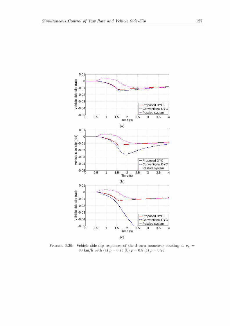
Simultaneous Control of Yaw Rate and Vehicle Side-Slip 127
0 0.5 1 1.5 2 2.5 3 3.5 4-0.05
-0.04
-0.03
-0.02
-0.01
0
0.01
Time (s)
Vehi
cle
side
-slip
(rad
)
Proposed DYCConventional DYCPassive system
(a)
0 0.5 1 1.5 2 2.5 3 3.5 4-0.05
-0.04
-0.03
-0.02
-0.01
0
0.01
Time (s)
Vehi
cle
side
-slip
(rad
)
Proposed DYCConventional DYCPassive system
(b)
0 0.5 1 1.5 2 2.5 3 3.5 4-0.05
-0.04
-0.03
-0.02
-0.01
0
0.01
Time (s)
Vehi
cle
side
-slip
(rad
)
Proposed DYCConventional DYCPassive system
(c)
Figure 6.29: Vehicle side-slip responses of the J-turn maneuver starting at vx =80 km/h with (a) ρ = 0.75 (b) ρ = 0.5 (c) ρ = 0.25.
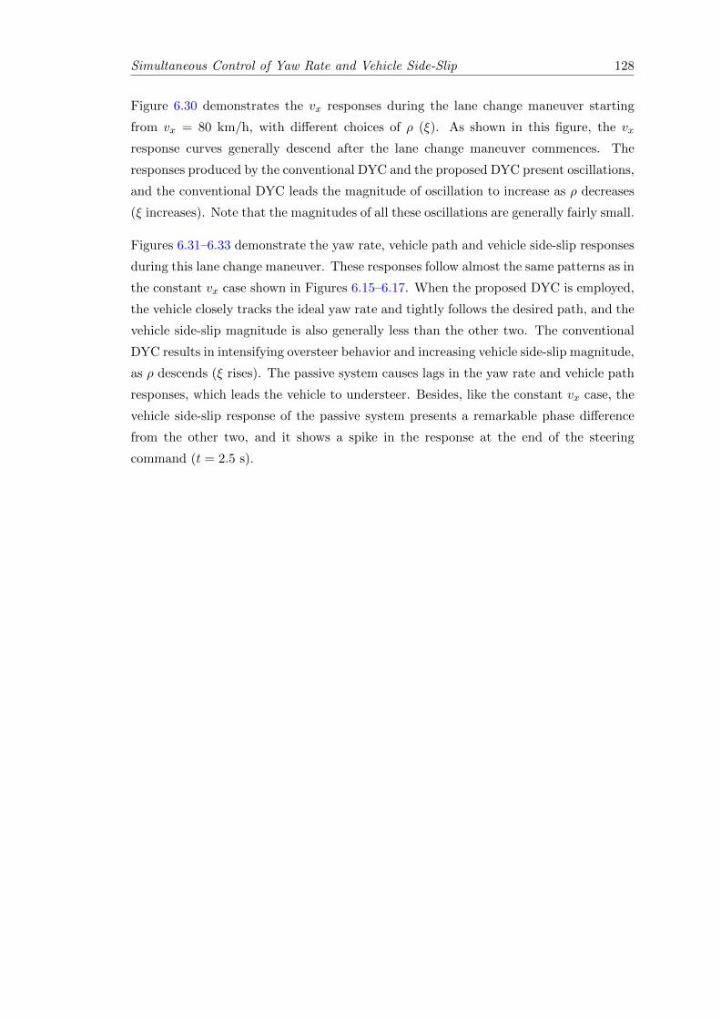
Simultaneous Control of Yaw Rate and Vehicle Side-Slip 128
Figure 6.30 demonstrates the vx responses during the lane change maneuver starting
from vx = 80 km/h, with different choices of ρ (ξ). As shown in this figure, the vx
response curves generally descend after the lane change maneuver commences. The
responses produced by the conventional DYC and the proposed DYC present oscillations,
and the conventional DYC leads the magnitude of oscillation to increase as ρ decreases
(ξ increases). Note that the magnitudes of all these oscillations are generally fairly small.
Figures 6.31–6.33 demonstrate the yaw rate, vehicle path and vehicle side-slip responses
during this lane change maneuver. These responses follow almost the same patterns as in
the constant vx case shown in Figures 6.15–6.17. When the proposed DYC is employed,
the vehicle closely tracks the ideal yaw rate and tightly follows the desired path, and the
vehicle side-slip magnitude is also generally less than the other two. The conventional
DYC results in intensifying oversteer behavior and increasing vehicle side-slip magnitude,
as ρ descends (ξ rises). The passive system causes lags in the yaw rate and vehicle path
responses, which leads the vehicle to understeer. Besides, like the constant vx case, the
vehicle side-slip response of the passive system presents a remarkable phase difference
from the other two, and it shows a spike in the response at the end of the steering
command (t = 2.5 s).
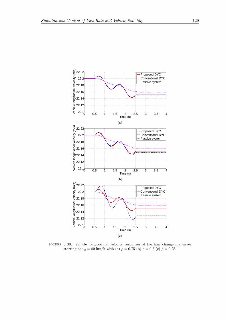
Simultaneous Control of Yaw Rate and Vehicle Side-Slip 129
0 0.5 1 1.5 2 2.5 3 3.5 422.1
22.12
22.14
22.16
22.18
22.2
22.22
Time (s)
Vehi
cle
long
itudi
nal v
eloc
ity (m
/s)
Proposed DYCConventional DYCPassive system
(a)
0 0.5 1 1.5 2 2.5 3 3.5 422.1
22.12
22.14
22.16
22.18
22.2
22.22
Time (s)
Vehi
cle
long
itudi
nal v
eloc
ity (m
/s)
Proposed DYCConventional DYCPassive system
(b)
0 0.5 1 1.5 2 2.5 3 3.5 422.1
22.12
22.14
22.16
22.18
22.2
22.22
Time (s)
Vehi
cle
long
itudi
nal v
eloc
ity (m
/s)
Proposed DYCConventional DYCPassive system
(c)
Figure 6.30: Vehicle longitudinal velocity responses of the lane change maneuverstarting at vx = 80 km/h with (a) ρ = 0.75 (b) ρ = 0.5 (c) ρ = 0.25.
Simultaneous Control of Yaw Rate and Vehicle Side-Slip 130
0 0.5 1 1.5 2 2.5 3 3.5 4-0.4
-0.2
0
0.2
0.4
Time (s)
Yaw
rate
(rad
/s)
IdealProposed DYCConventional DYCPassive system
(a)
0 0.5 1 1.5 2 2.5 3 3.5 4-0.4
-0.2
0
0.2
0.4
Time (s)
Yaw
rate
(rad
/s)
IdealProposed DYCConventional DYCPassive system
(b)
0 0.5 1 1.5 2 2.5 3 3.5 4-0.4
-0.2
0
0.2
0.4
Time (s)
Yaw
rate
(rad
/s)
IdealProposed DYCConventional DYCPassive system
(c)
Figure 6.31: Yaw rate responses of the lane change maneuver starting at vx =80 km/h with (a) ρ = 0.75 (b) ρ = 0.5 (c) ρ = 0.25.
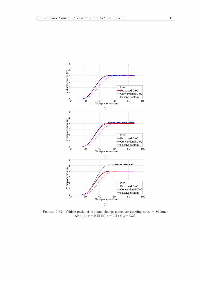
Simultaneous Control of Yaw Rate and Vehicle Side-Slip 131
0 20 40 60 80 1000
1
2
3
4
5
6
X-displacement (m)
Y-di
spla
cem
ent (
m)
IdealProposed DYCConventional DYCPassive system
(a)
0 20 40 60 80 1000
1
2
3
4
5
6
X-displacement (m)
Y-di
spla
cem
ent (
m)
IdealProposed DYCConventional DYCPassive system
(b)
0 20 40 60 80 1000
1
2
3
4
5
6
X-displacement (m)
Y-di
spla
cem
ent (
m)
IdealProposed DYCConventional DYCPassive system
(c)
Figure 6.32: Vehicle paths of the lane change maneuver starting at vx = 80 km/hwith (a) ρ = 0.75 (b) ρ = 0.5 (c) ρ = 0.25.
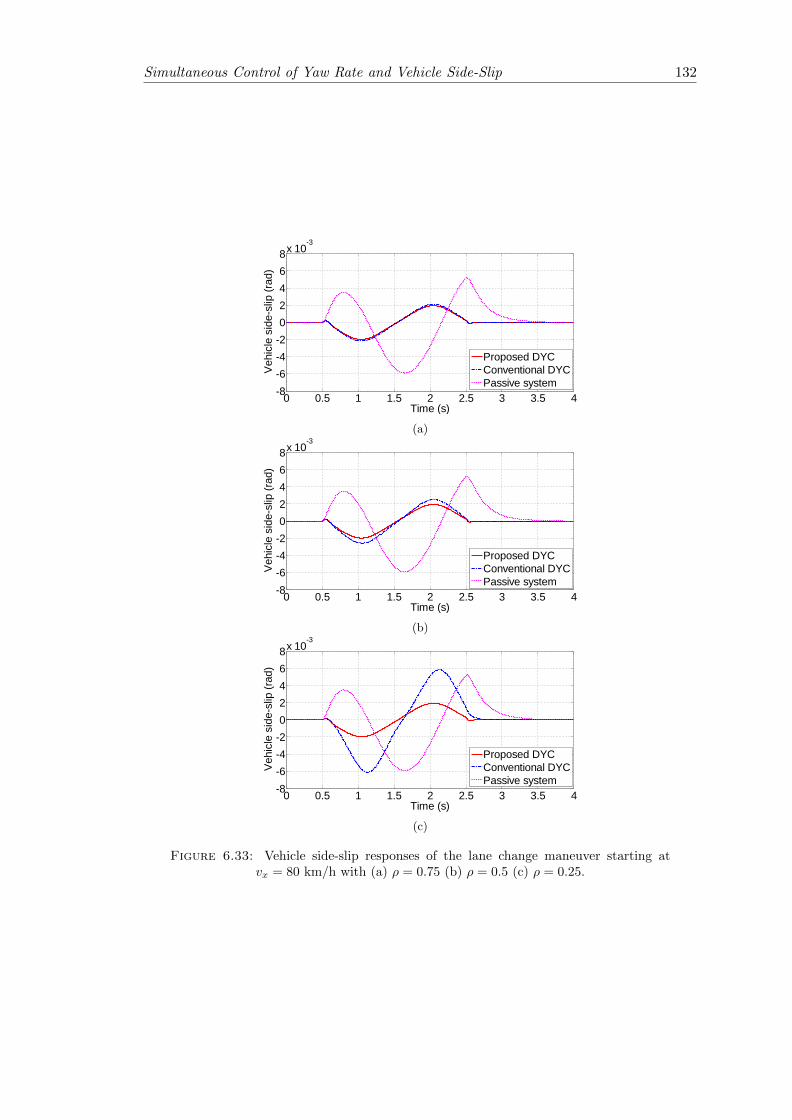
Simultaneous Control of Yaw Rate and Vehicle Side-Slip 132
0 0.5 1 1.5 2 2.5 3 3.5 4-8-6-4-202468x 10
-3
Time (s)
Vehi
cle
side
-slip
(rad
)
Proposed DYCConventional DYCPassive system
(a)
0 0.5 1 1.5 2 2.5 3 3.5 4-8-6-4-202468x 10
-3
Time (s)
Vehi
cle
side
-slip
(rad
)
Proposed DYCConventional DYCPassive system
(b)
0 0.5 1 1.5 2 2.5 3 3.5 4-8-6-4-202468x 10
-3
Time (s)
Vehi
cle
side
-slip
(rad
)
Proposed DYCConventional DYCPassive system
(c)
Figure 6.33: Vehicle side-slip responses of the lane change maneuver starting atvx = 80 km/h with (a) ρ = 0.75 (b) ρ = 0.5 (c) ρ = 0.25.
Simultaneous Control of Yaw Rate and Vehicle Side-Slip 133
6.4 SUMMARY
In this chapter, a novel sliding mode DYC design for simultaneous control of the yaw
rate and vehicle side-slip is presented. The proposed sliding mode controller employs a
linear combination of the normalized absolute values of the yaw rate and vehicle side-slip
errors as the switching function. The complete nonlinear vehicle equations of motion
derived in Chapter 3 are employed to formulate the sliding mode control command.
Extensive comparative simulations are conducted to verify the effectiveness of the pro-
posed DYC scheme. In the simulation studies, the vehicle undergoes the J-turn and lane
change maneuvers with constant or uncontrolled vehicle longitudinal velocities. The
simulation results demonstrate that the proposed DYC solution clearly outperforms the
compared methods in terms of achieving close-to-neutral steer characteristic, tracking
the ideal vehicle path, and obtaining smaller magnitude of vehicle side-slip.
Chapter 7
Conclusions and
Recommendations
7.1 CONCLUSIONS
Direct yaw moment control systems produce a corrective yaw moment to achieve en-
hanced vehicle handling and stability, by means of individual control of longitudinal tire
forces (braking and/or traction forces). Conventionally, DYC systems were commonly
realized in the form of braking-based VSC systems or active differentials, either of which
presents certain types of downsides. Since the advent of electric vehicles (or hybrid ve-
hicles) equipped with independent driving motors, the latest type of DYC using electric
motors to generate the corrective yaw moment has become a research focus. This new
DYC type presents several apparent advantages over the conventional DYC schemes,
and its effectiveness in enhancing the vehicle handling and stability has been verified by
the published works.
Most existing DYC schemes adopt the yaw rate and/or vehicle side-slip as the main
control variable(s), as these two vehicle states are known to be the fundamental states
that govern the vehicle handling and stability. The scope of this study has been focused
on the analysis and design of the latest DYC type for electric vehicles (or hybrid vehicles)
with independent driving motors, employing the yaw rate and/or vehicle side-slip as the
control variable(s).
This thesis has looked into a wide range of existing vehicle dynamics control designs,
ranging from the basic and straightforward solutions to the state-of-the-art DYC schemes.
In a detailed literature review, the theories used in the control techniques were explained
and the characteristics of each control scheme were highlighted. Then, a full vehicle
134
Conclusions and Recommendations 135
model including the vehicle equivalent mechanical model, vehicle equations of motion,
wheel equation of motion and Magic Formula tire model was established. On the basis
of the literature review and full vehicle model, three types of DYC systems have been
proposed with detailed design processes and simulation verifications. These systems are
the yaw rate-based DYC, vehicle side-slip-based DYC and simultaneous control of the
yaw rate and vehicle side-slip.
To clarify the basic question on how the corrective yaw moment generated by a DYC
system changes the vehicle dynamics, a mathematical relationship was derived from the
vehicle equations of motion to show how the steady-state yaw rate response depends on
the torque difference between the two driving motors (i.e. the corrective yaw moment).
This relationship implies that the steady-state yaw rate can be directly controlled by
tuning the torque difference to achieve a reference value. Based on this relationship, a
yaw rate-based DYC system was designed to track the desired neutral steer yaw rate
response. Comparative simulation results show that the vehicle closely traces the desired
yaw rate with the proposed DYC on-board, and the vehicle handling is significantly
improved.
Similarly, another mathematical relationship was derived to reveal the effect of a DYC
system on the other crucial vehicle state, vehicle side-slip. This relationship demon-
strates that the steady-state vehicle side-slip is a function of the torque difference be-
tween the left and right driving motors. On the basis of this relationship, a vehicle
side-slip-based DYC solution was proposed to achieve zero vehicle side-slip. Simulation
results manifest that the vehicle side-slip is minimized by the proposed DYC system.
As a result, the vehicle stability and driver’s sense of control are greatly enhanced.
After dealing with the yaw rate and vehicle side-slip individually, an integrated sliding
mode control scheme which employs the yaw rate and vehicle side-slip simultaneously as
the control variables was devised. This design introduces a novel switching function that
guarantees the simultaneous convergences of both the yaw rate and vehicle side-slip er-
rors to zero, and eliminates the limitations presented in the common sliding mode DYC
solutions. Extensive simulations demonstrate that the proposed sliding mode DYC ap-
proach is effective in suppressing both the yaw rate and vehicle side-slip errors in various
driving scenarios, and it outperforms the common sliding mode DYC schemes in terms
of tracking the desired yaw rate, vehicle path and vehicle side-slip. The simultaneous
regulation of the yaw rate and vehicle side-slip by the proposed DYC method effectively
enhances both the vehicle handling and stability.
Conclusions and Recommendations 136
7.2 RECOMMENDATIONS
Throughout this thesis, all research questions raised in Chapter 1 have been answered
and the research objectives have been achieved. However, in the light of the work carried
out in this study, some possible areas are thought worthy of further investigation.
It is recommended that experimentation be performed to validate and improve the pro-
posed schemes further. For each control method, firstly, Hardware-In-the-Loop (HIL)
simulations should be conducted to check and regulate the control law in the Electronic
Control Unit (ECU). Then, field tests should be performed using the same vehicle ma-
neuvers as in the simulations to evaluate the control scheme thoroughly. Based on the
HIL simulation and field testing results, possible adjustments and improvements can be
made to the control design.
The scope of this study has been narrowed down to the DYC systems for electric vehi-
cles (or hybrid vehicles) with two rear independent driving motors. The control schemes
proposed in this thesis can also be applied to 4WD electric vehicles. With four inde-
pendent driving motors on-board, the problem of appropriate distribution of the motor
torques to generate a certain corrective yaw moment needs to be tackled. The proposed
DYC methods for 2-Wheel-Drive (2WD) vehicles, also known as the upper level control,
can be employed to compute the target corrective yaw moment for 4WD vehicles. Then
this yaw moment should be realized by allocating an appropriate torque to each driving
motor based on the torque distribution strategy. So far, a large number of upper level
control methods have been proposed, however there are not sufficient torque distribution
strategies available in the literature. It is suggested that further research be conducted
to design an effective torque distribution strategy, in order to extend the proposed upper
level control schemes to 4WD electric vehicles.
In the recent literature, some control solutions integrate DYC system with other types
of vehicle dynamics control systems such as AFS, 4WS and ARCS. It is known that a
certain vehicle dynamics control system is most effective in a specific region. The inte-
grated control systems take advantage of each type of vehicle dynamics control system,
and ensure satisfactory control performance in a wide range of driving condition. The
proposed DYC methods in this thesis are able to work in tandem with other vehicle
dynamics control systems, and the design of an appropriate integrating strategy should
be studied in the future.
Furthermore, a challenge confronted in this study is that different vehicle equations of
motion and tire models are available in the literature, and they need to be carefully
selected, combined and possibly modified to establish a suitable full vehicle model. The
experience learned from this challenge is that the subsystems in the full vehicle model
Conclusions and Recommendations 137
must be mathematically and physically compatible, i.e. they do not contradict each
other. It is also suggested that computer simulations of different full vehicle models
be performed, and the simulation results be compared with the field test data to check
the validity of these vehicle models. By this means, an optimal full vehicle model can
possibly be found out.
Last but not least, there are not sufficient review articles available in the literature
introducing DYC designs for electric and hybrid vehicles with independent motors. It is
recommended that comprehensive review papers be written to sum up the state-of-the-
art DYC designs, in order to facilitate further research in this field.
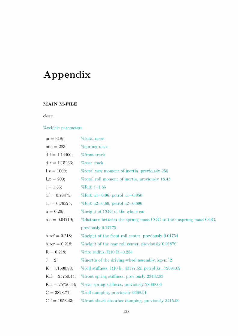
Appendix
MAIN M-FILE
clear;
%vehicle parameters
m = 318; %total mass
m s = 283; %sprung mass
d f = 1.14400; %front track
d r = 1.15266; %rear track
I z = 1000; %total yaw moment of inertia, previously 250
I x = 200; %total roll moment of inertia, previously 18.43
l = 1.55; %R10 l=1.65
l f = 0.78475; %R10 a1=0.96, petrol a1=0.850
l r = 0.76525; %R10 a2=0.69, petrol a2=0.696
h = 0.26; %height of COG of the whole car
h s = 0.04719; %distance between the sprung mass COG to the unsprung mass COG,
previously 0.27175
h rcf = 0.218; %height of the front roll center, previously 0.01754
h rcr = 0.218; %height of the rear roll center, previously 0.01876
R = 0.218; %tire radius, R10 R=0.254
J = 2; %inertia of the driving wheel assembly, kg∗mˆ2
K = 51500.88; %roll stiffness, R10 k=40177.52, petrol kr=72694.02
K f = 25750.44; %front spring stiffness, previously 23432.83
K r = 25750.44; %rear spring stiffness, previously 28068.06
C = 3828.71; %roll damping, previously 6668.91
C f = 1953.43; %front shock absorber damping, previously 3415.09
138
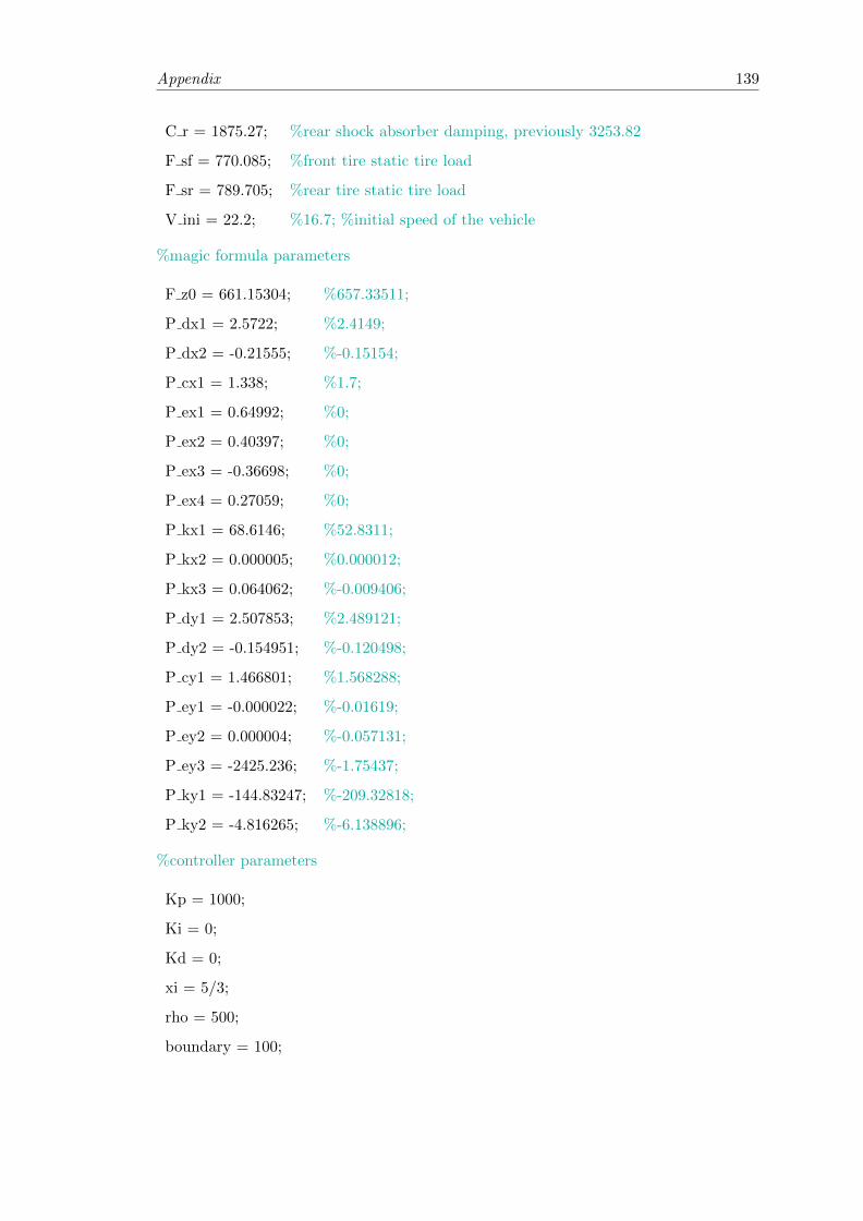
Appendix 139
C r = 1875.27; %rear shock absorber damping, previously 3253.82
F sf = 770.085; %front tire static tire load
F sr = 789.705; %rear tire static tire load
V ini = 22.2; %16.7; %initial speed of the vehicle
%magic formula parameters
F z0 = 661.15304; %657.33511;
P dx1 = 2.5722; %2.4149;
P dx2 = -0.21555; %-0.15154;
P cx1 = 1.338; %1.7;
P ex1 = 0.64992; %0;
P ex2 = 0.40397; %0;
P ex3 = -0.36698; %0;
P ex4 = 0.27059; %0;
P kx1 = 68.6146; %52.8311;
P kx2 = 0.000005; %0.000012;
P kx3 = 0.064062; %-0.009406;
P dy1 = 2.507853; %2.489121;
P dy2 = -0.154951; %-0.120498;
P cy1 = 1.466801; %1.568288;
P ey1 = -0.000022; %-0.01619;
P ey2 = 0.000004; %-0.057131;
P ey3 = -2425.236; %-1.75437;
P ky1 = -144.83247; %-209.32818;
P ky2 = -4.816265; %-6.138896;
%controller parameters
Kp = 1000;
Ki = 0;
Kd = 0;
xi = 5/3;
rho = 500;
boundary = 100;

Appendix 140
%start simulation
open system(‘new control model 7.mdl’);
sim(‘new control model 7.mdl’);
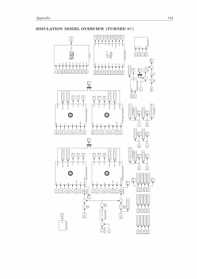
Appendix 141
SIMULATION MODEL OVERVIEW (TURNED 90◦)
V_x
V_y
r delta V
ehic
le P
ath
delta
F_x1
F_x2
F_x3
F_x4
F_y1
F_y2
F_y3
F_y4
V_x
V_y
r p
phi
beta
F_xs
um F_yf
F_yr
Veh
icle
Dyn
amic
s
r_ne
w_0
75_5
00_1
00
To
Wor
kspa
ce3
V_x
_new
_075
_500
_100
To
Wor
kspa
ce2
beta
_new
_075
_500
_100
To
Wor
kspa
ce1
Out
1
Ste
erin
g A
ngle
erro
rB
ase
Torq
ue
Spe
ed C
ontro
ller
1
Slid
erG
ain2
1
Slid
erG
ain11
Slid
erG
ain
Sat
urat
ion1
Sat
urat
ion
V_x
V_y
r phi
p F_xs
um
F_yr
mot
or to
rque
F_x3
F_y3
F_z3
slip
_rat
io
side
_slip
omeg
a
Rea
r Rig
ht T
ire D
ynam
ics
V_x
V_y
r phi
p F_xs
um
F_yr
mot
or to
rque
omeg
a
slip
_rat
io
side
_slip
F_z4
F_x4
F_y4
Rea
r Lef
t Tire
Dyn
amic
s
V_i
ni
Initi
al S
peed
[p]
[r_d]
[F_y
3]
[F_x
3]
[F_y
4]
[F_x
4]
[r]
[F_y
r]
[F_y
f]
[F_x
sum
]
[bet
a]
[V_y
]
[F_y
1]
[F_z
3]
[F_y
2]
[F_x
2]
[F_z
2]
[phi
]
[F_z
4][F
_z1]
[F_x
1]
[del
ta_T
]
[V_x
]
[del
ta]
xi Gai
n
delta
V_x
V_y
r phi
p F_xs
um
F_yf
F_x2
F_y2
F_z2
slip
_rat
io
side
_slip
omeg
a
Fron
t Rig
ht T
ire D
ynam
ics
delta
V_x
V_y
r phi
p F_xs
um
F_yf
omeg
a
slip
_rat
io
side
_slip
F_z1
F_x1
F_y1
Fron
t Lef
t Tire
Dyn
amic
s
[r]
[r]
[del
ta]
[F_y
4]
[F_y
3]
[F_y
2]
[F_y
1]
[phi
]
[del
ta_T
]
[del
ta_T
]
[F_x
2]
[F_x
1]
[bet
a]
[r_d][r]
[r]
[V_x
]
[V_y
]
[p]
[V_y
]
[bet
a]
[F_x
1]
[F_x
sum
]
[F_x
sum
]
[F_y
r]
[F_y
r]
[V_x
]
[F_y
f]
[r]
[del
ta]
[F_x
sum
]
[F_y
f]
[V_x
]
[F_y
4]
[F_y
3]
[F_x
sum
]
[F_y
2]
[F_y
1]
[F_x
4]
[F_x
3]
[F_z
4]
[F_z
3]
[F_z
2]
[V_x
]
[F_y
4]
[F_y
3]
[F_y
2]
[F_y
1][p
]
[p]
[V_x
]
[p]
[phi
]
[phi
][V
_x]
[F_z
1]
[F_x
2]
[phi
]
[p]
[F_x
4]
[F_x
3]
[F_x
2]
[F_x
1]
[r]
[V_y
]
[bet
a]
[del
ta]
[V_x
]
[r]
[V_y
]
[del
ta]
[V_x
]
[del
ta]
[phi
]
[r]
[V_y
]
[V_y
][d
elta
]
delta
V_x
r_d
Des
ired
Yaw
Rat
e
r r_d
beta
delta
F_x1
F_x2
F_y1
F_y2
F_y3
F_y4
delta
_T
Con
trolle
r
|u|
Abs
1
|u|
Abs
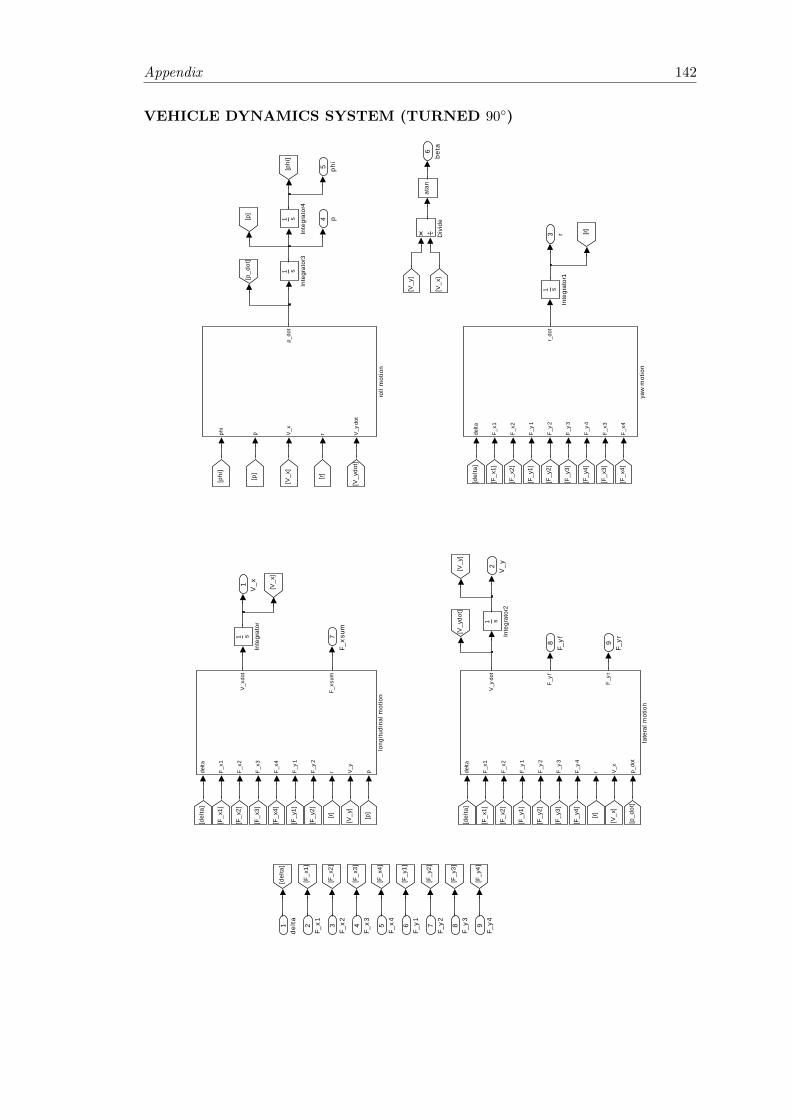
Appendix 142
VEHICLE DYNAMICS SYSTEM (TURNED 90◦)
9F_
yr8F_
yf7F_
xsum
6be
ta
5 phi
4 p
3 r
2V
_y
1V
_x
delta
F_x
1
F_x
2
F_y1
F_y2
F_y3
F_y4
F_x
3
F_x
4
r_do
t
yaw
mot
ion
phi
p V_x
r V_y
dot
p_do
t
roll
mot
ion
delta
F_x
1
F_x
2
F_x
3
F_x
4
F_y1
F_y2
r V_y
p
V_x
dot
F_x
sum
long
itudi
nal m
otio
n
delta
F_x
1
F_x
2
F_y1
F_y2
F_y3
F_y4
r V_x
p_do
t
V_y
dot
F_yf
F_yr
late
ral m
otio
n
atan
1 s
Inte
grat
or4
1 s
Inte
grat
or3
1 s
Inte
grat
or2
1 s
Inte
grat
or1
1 s
Inte
grat
or
[F_x
3]
[F_x
2]
[F_x
1]
[del
ta]
[p]
[phi
]
[V_x
]
[V_y
][V
_ydo
t]
[p_d
ot]
[F_y
4]
[F_y
3]
[F_y
2]
[F_y
1]
[F_x
4]
[r]
[F_y
2]
[F_y
1]
[F_x
2]
[F_x
1]
[F_x
2]
[p_d
ot]
[F_y
1]
[p]
[F_x
4]
[F_x
3][V
_x]
[r]
[F_y
4]
[F_y
3]
[F_x
2]
[del
ta]
[F_y
4]
[F_y
3]
[F_y
2]
[del
ta]
[V_x
]
[V_y
]
[F_y
2]
[V_y
]
[r]
[F_x
1]
[V_y
dot]
[del
ta]
[phi
]
[p]
[V_x
]
[r]
[F_y
1]
[F_x
4]
[F_x
3]
[F_x
1]
Div
ide
9F_
y48F_
y37F_
y26F_
y15F_
x44F_
x33F_
x22F_
x11de
lta
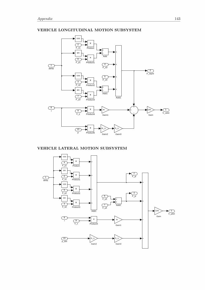
Appendix 143
VEHICLE LONGITUDINAL MOTION SUBSYSTEM
2F_xsum
1V_xdot
sin
cos
sin
cos
Product5
Product4
Product3
Product2
Product1
Product
h_s
Gain3
m_s
Gain2
m
Gain1
1/m
Gain
Add2
Add1
Add
10p
9V_y
8r
7F_y2
6F_y1
5F_x4
4F_x3
3F_x2
2F_x1
1delta
VEHICLE LATERAL MOTION SUBSYSTEM
3F_yr
2F_yf
1V_ydot
sin
cos
sin
cos
Product4
Product3
Product2
Product1
Product
h_s
Gain3
m_s
Gain2
m
Gain1
1/m
Gain
Add2
Add1
10p_dot
9V_x
8r
7F_y4
6F_y3
5F_y2
4F_y1
3F_x2
2F_x1
1delta
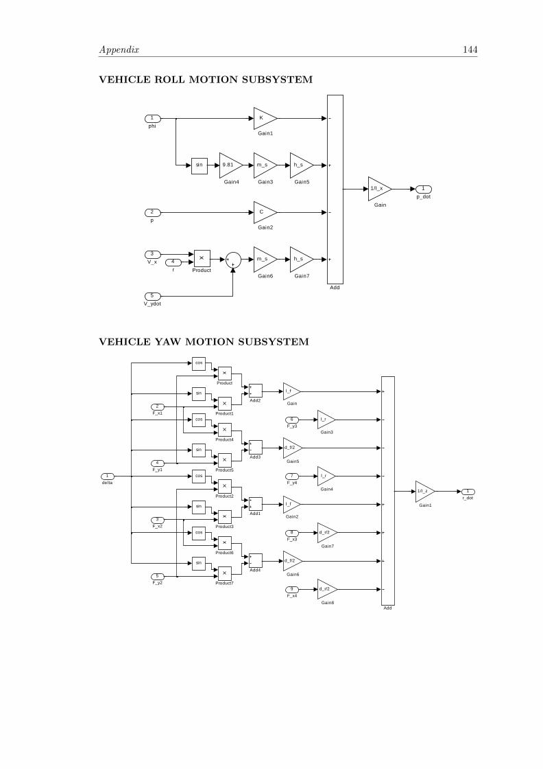
Appendix 144
VEHICLE ROLL MOTION SUBSYSTEM
1p_dot
sin
Product
h_s
Gain7
m_s
Gain6
h_s
Gain5
9.81
Gain4
m_s
Gain3
C
Gain2
K
Gain1
1/I_x
Gain
Add5
V_ydot
4r
3V_x
2p
1phi
VEHICLE YAW MOTION SUBSYSTEM
1r_dot
sin
cos
sin
cos
sin
cos
sin
cos
Product7
Product6
Product5
Product4
Product3
Product2
Product1
Product
d_r/2
Gain8
d_r/2
Gain7
d_f/2
Gain6
d_f/2
Gain5
l_r
Gain4
l_r
Gain3
l_f
Gain2
1/I_z
Gain1
l_f
Gain
Add4
Add3
Add2
Add1
Add
9F_x4
8F_x3
7F_y4
6F_y3
5F_y2
4F_y1
3F_x2
2F_x1
1delta
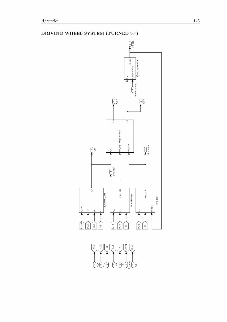
Appendix 145
DRIVING WHEEL SYSTEM (TURNED 90◦)
6F_
y4 5F_
x4
4F_
z4
3si
de_s
lip
2sl
ip_r
atio
1om
ega
F_x
mo
tor
torq
ue
om
ega
Whe
el d
ynam
ics
V_x
r om
ega
slip
_ra
tio
Tire
Slip
V_y
V_x
r
side
_slip
Tire
Sid
eslip
F_x
sum
F_yr
phi
p
F_z4
RL_
Nor
mal
_Loa
d
[F_y
r]
[p]
[phi
]
[r]
[V_y
]
[F_x
sum
]
[V_x
]
[F_y
r]
[r]
[V_x
]
[r]
[V_x
]
[V_y
]
[F_x
sum
]
[phi
]
[p]
F_z
side
_slip
slip
_rat
io
F_y
F_x
Mag
ic_F
orm
ula
8m
otor
tor
que
7F_
yr6F_
xsum5 p4 phi
3 r2V
_y1V
_x
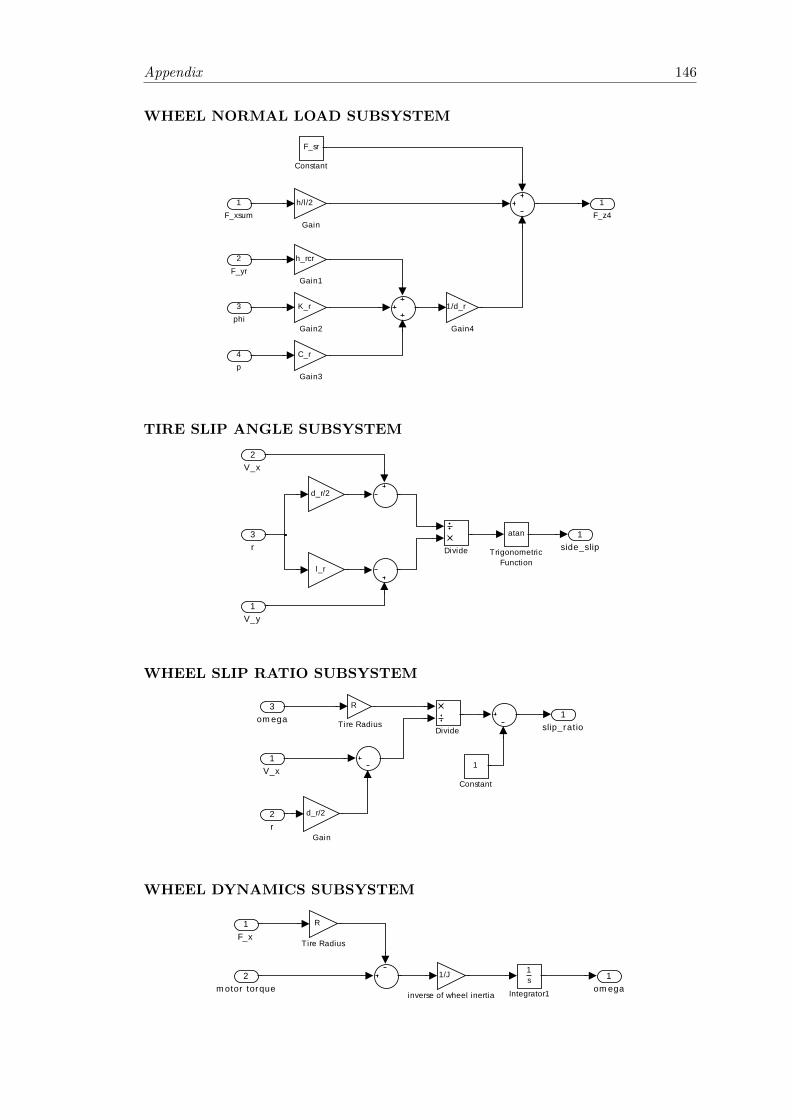
Appendix 146
WHEEL NORMAL LOAD SUBSYSTEM
1F_z4
1/d_r
Gain4
C_r
Gain3
K_r
Gain2
h_rcr
Gain1
h/l/2
Gain
F_sr
Constant
4p
3phi
2F_yr
1F_xsum
TIRE SLIP ANGLE SUBSYSTEM
1side_slip
atan
TrigonometricFunction
l_r
d_r/2
Divide
3r
2V_x
1V_y
WHEEL SLIP RATIO SUBSYSTEM
1slip_ratio
R
Tire Radius
d_r/2
Gain
Divide
1
Constant
3omega
2r
1V_x
WHEEL DYNAMICS SUBSYSTEM
1omega
1/J
inverse of wheel inertia
R
Tire Radius
1s
Integrator1
2motor torque
1F_x
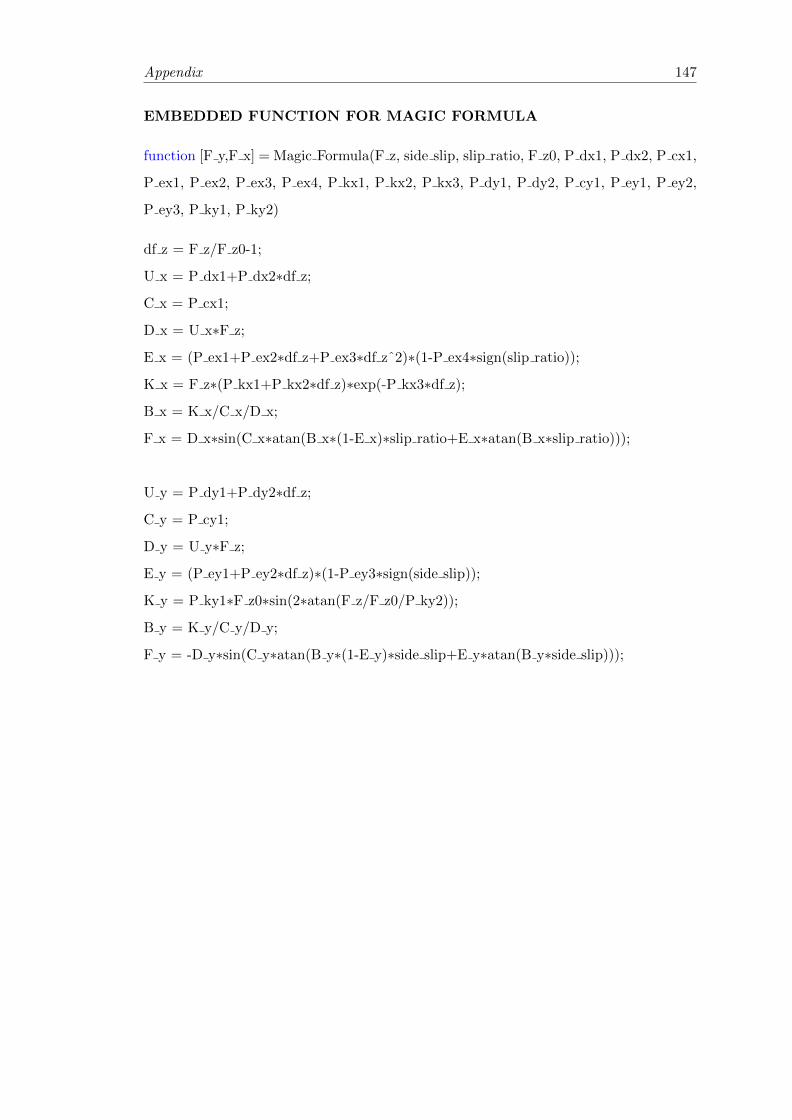
Appendix 147
EMBEDDED FUNCTION FOR MAGIC FORMULA
function [F y,F x] = Magic Formula(F z, side slip, slip ratio, F z0, P dx1, P dx2, P cx1,
P ex1, P ex2, P ex3, P ex4, P kx1, P kx2, P kx3, P dy1, P dy2, P cy1, P ey1, P ey2,
P ey3, P ky1, P ky2)
df z = F z/F z0-1;
U x = P dx1+P dx2∗df z;
C x = P cx1;
D x = U x∗F z;
E x = (P ex1+P ex2∗df z+P ex3∗df zˆ2)∗(1-P ex4∗sign(slip ratio));
K x = F z∗(P kx1+P kx2∗df z)∗exp(-P kx3∗df z);
B x = K x/C x/D x;
F x = D x∗sin(C x∗atan(B x∗(1-E x)∗slip ratio+E x∗atan(B x∗slip ratio)));
U y = P dy1+P dy2∗df z;
C y = P cy1;
D y = U y∗F z;
E y = (P ey1+P ey2∗df z)∗(1-P ey3∗sign(side slip));
K y = P ky1∗F z0∗sin(2∗atan(F z/F z0/P ky2));
B y = K y/C y/D y;
F y = -D y∗sin(C y∗atan(B y∗(1-E y)∗side slip+E y∗atan(B y∗side slip)));
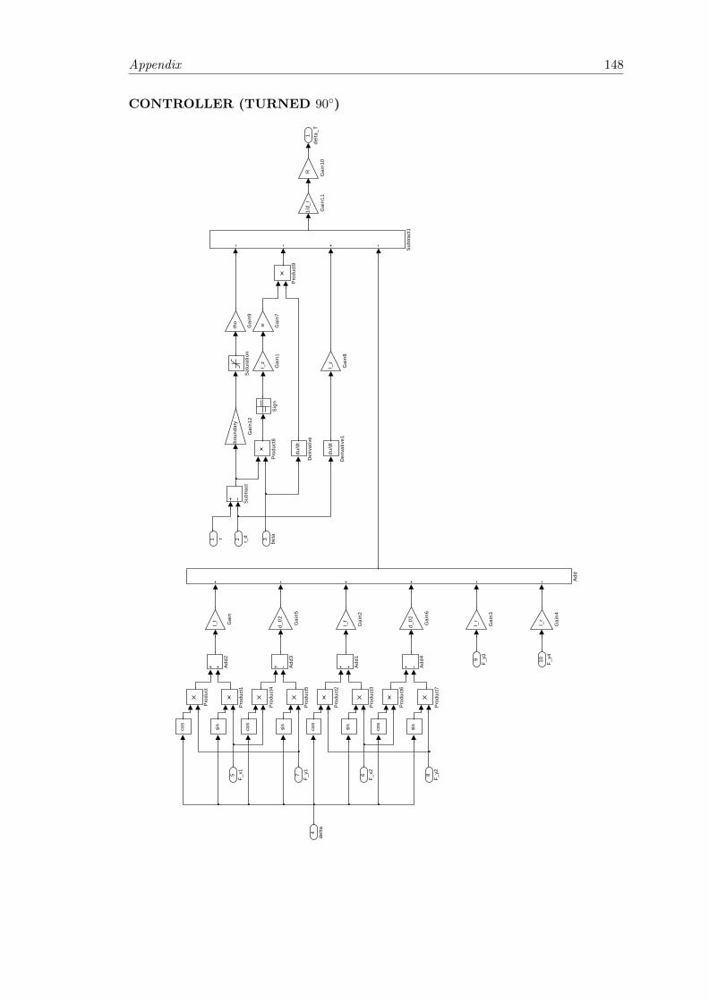
Appendix 148
CONTROLLER (TURNED 90◦)
1de
lta_T
sin
cos
sin
cos
sin
cos
sin
cos
Sub
tract
1
Sub
tract
Sig
n
Sat
urat
ion
Pro
duct
9
Pro
duct
8
Pro
duct
7
Pro
duct
6
Pro
duct
5
Pro
duct
4
Pro
duct
3
Pro
duct
2
Pro
duct
1
Pro
duct
rho
Gai
n9
I_z
Gai
n8
xi Gai
n7
d_f/2
Gai
n6
d_f/2
Gai
n5
l_r
Gai
n4
l_r
Gai
n3
l_f
Gai
n2
boun
dary
Gai
n12
1/d_
r
Gai
n11
R Gai
n10
I_z
Gai
n1
l_f Gai
n
du/d
t
Der
ivat
ive1
du/d
t
Der
ivat
ive
Add
4
Add
3
Add
2
Add
1
Add
10 F_y49
F_y3
8F_
y27F_
y1 6F_
x25F_
x1
4de
lta
3be
ta2 r_d1 r
Bibliography
[1] M. Nagai, Y. Hirano, and S. Yamanaka, “Integrated control of active rear wheel
steering and direct yaw moment control,” Vehicle System Dynamics, vol. 27, no.
5-6, pp. 357–370, 1997.
[2] M. Aga and A. Okada, “Analysis of vehicle stability control (VSC)’s effectiveness
from accident data,” in Proceedings - 18th International Technical Conference on
the Enhanced Safety of Vehicles, ESV 2003, no. 541, Wahington, DC, United
States, 2003.
[3] A. Lie, C. Tingvall, M. Krafft, and A. Kullgren, “The effectiveness of electronic
stability control (ESC) in reducing real life crashes and injuries,” Traffic Injury
Prevention, vol. 7, no. 1, pp. 38–43, 2006.
[4] A. Chouinard and J.-F. Lecuyer, “A study of the effectiveness of electronic
stability control in canada,” Accident Analysis and Prevention, vol. 43, no. 1, pp.
451–460, 2011.
[5] E. K. Liebemann, K. Meder, J. Schuh, and G. Nenninger, “Safety and
performance enhancement: The bosch electronic stability control (ESP),” SAE
Technical Paper 2004-21-0060, 2004.
[6] A. T. van Zanten, “Bosch ESP systems: 5 years of experience,” SAE Technical
Paper 2000-01-1633, 2000.
[7] B. Mashadi, S. Mostaani, and M. Majidi, “Vehicle stability enhancement by
using an active differential,” Proceedings of the Institution of Mechanical
Engineers. Part I: Journal of Systems and Control Engineering, vol. 225, no. 8,
pp. 1098–1114, 2011.
149
Bibliography 150
[8] M. Hancock, R. Williams, E. Fina, and M. Best, “Yaw motion control via active
differentials,” Transactions of the Institute of Measurement and Control, vol. 29,
no. 2, pp. 137–157, 2007.
[9] M. Canale, L. Fagiano, A. Ferrara, and C. Vecchio, “Vehicle yaw control via
second-order sliding-mode technique,” IEEE Transactions on Industrial
Electronics, vol. 55, no. 11, pp. 3908–3916, 2008.
[10] M. Hancock, R. Williams, T. Gordon, and M. Best, “A comparison of braking
and differential control of road vehicle yaw-sideslip dynamics,” Proceedings of the
Institution of Mechanical Engineers, Part D: Journal of Automobile Engineering,
vol. 219, no. 3, pp. 309–327, 2005.
[11] M. Canale, L. Fagiano, M. Milanese, and P. Borodani, “Robust vehicle yaw
control using an active differential and imc techniques,” Control Engineering
Practice, vol. 15, no. 8, pp. 923–941, 2007.
[12] Y. Ushiroda, K. Sawase, N. Takahashi, K. Suzuki, and K. Manabe, “Development
of super AYC,” Mitsubishi Motors Technical Review, vol. 15, pp. 73–76, 2003.
[13] N. Mutoh, “Driving and braking torque distribution methods for front- and
rear-wheel-independent drive-type electric vehicles on roads with low friction
coefficient,” IEEE Transactions on Industrial Electronics, vol. 59, no. 10, pp.
3919 – 3933, 2012.
[14] C. Fu, R. Hoseinnezhad, A. Bab-Hadiashar, and R. N. Jazar, “Direct yaw
moment control for electric and hybrid vehicles with independent motors,”
International Journal of Vehicle Design, 2014, accepted.
[15] Y. Chen, J. Hedrick, and K. Guo, “A novel direct yaw moment controller for
in-wheel motor electric vehicles,” Vehicle System Dynamics, vol. 51, no. 6, pp.
925–942, 2013.
[16] C. Fu, R. Hoseinnezhad, A. Bab-Hadiashar, R. N. Jazar, and S. Watkins,
“Electronic differential for high-performance electric vehicles with independent
driving motors,” International Journal of Electric and Hybrid Vehicles, vol. 6,
no. 2, pp. 108–132, 2014.
Bibliography 151
[17] K. Uematsu and J. C. Gerdes, “A comparison of several sliding surfaces for
stability control,” in Proceedings - 6th International Symposium on Advanced
Vehicle Control, AVEC 2002, Hiroshima, Japan, 2002, pp. 601–608.
[18] A. T. van Zanten, R. Erhardt, G. Pfaff, F. Kost, U. Hartmann, and T. Ehret,
“Control aspects of the bosch-VDC,” in Proceedings - 3rd International
Symposium on Advanced Vehicle Control, AVEC 1996, Aachen, Germany, 1996,
pp. 573–608.
[19] A. T. van Zanten, R. Erhardt, and G. Pfaff, “VDC, the vehicle dynamics control
system of bosch,” SAE Technical Paper 950759, 1995.
[20] R. N. Jazar, Vehicle Dynamics: Theory and Application. Springer, 2008, ch. 10,
pp. 597–631.
[21] Y. Shibahata, K. Shimada, and T. Tomari, “Improvement of vehicle
maneuverability by direct yaw moment control,” Vehicle System Dynamics,
vol. 22, no. 5-6, pp. 465–481, 1993.
[22] C. Fu, R. Hoseinnezhad, R. Jazar, A. Bab-Hadiashar, and S. Watkins,
“Electronic differential design for vehicle side-slip control,” in Proceedings - 2012
International Conference on Control, Automation and Information Sciences,
ICCAIS 2012, Ho Chi Minh City, Vietnam, 2012, pp. 306 – 310.
[23] K. Yi, T. Chung, J. Kim, and S. Yi, “An investigation into differential braking
strategies for vehicle stability control,” Proceedings of the Institution of
Mechanical Engineers, Part D: Journal of Automobile Engineering, vol. 217,
no. 12, pp. 1081–1093, 2003.
[24] R. Tchamna and I. Youn, “Yaw rate and side-slip control considering vehicle
longitudinal dynamics,” International Journal of Automotive Technology, vol. 14,
no. 1, pp. 53–60, 2013.
[25] K. R. Buckholtz, “Use of fuzzy logic in wheel slip assignment - part I: Yaw rate
control,” SAE Technical Paper 2002-01-1221, 2002.
[26] ——, “Use of fuzzy logic in wheel slip assignment - part II: Yaw rate control with
sideslip angle limitation,” SAE Technical Paper 2002-01-1220, 2002.
Bibliography 152
[27] G. A. Magallan, C. H. De Angelo, G. Bisheimer, and G. Garcıa, “A
neighborhood electric vehicle with electronic differential traction control,” in
Proceedings - 34th Annual Conference of the IEEE Industrial Electronics Society,
IECON 2008, Orlando, FL, United states, 2008, pp. 2757–2763.
[28] G. Magallan, C. De Angelo, and G. Garcıa, “A neighbourhood-electric vehicle
development with individual traction on rear wheels,” International Journal of
Electric and Hybrid Vehicles, vol. 2, no. 2, pp. 115–136, 2009.
[29] P. M. Kelecy and R. D. Lorenz, “Control methodology for single inverter,
parallel connected dual induction motor drives for electric vehicles,” in
Proceedings - Power Electronics Specialists Conference, PESC’94 Record., 25th
Annual IEEE, vol. 2, Taipei, Taiwan, 1994, pp. 987–991.
[30] F. Profumo, Z. Zhang, and A. Tenconi, “Axial flux machines drives: A new
viable solution for electric cars,” IEEE Transactions on Industrial Electronics,
vol. 44, no. 1, pp. 39–45, 1997.
[31] D. Platt and B. Smith, “Twin rotor drive for an electric vehicle,” IEE
Proceedings B: Electric Power Applications, vol. 140, no. 2, pp. 131–138, 1993.
[32] ——, “A twin, composite, axial flux induction machine for an electric vehicle
drive,” in Proceedings - Electric Energy Conference 1987: An International
Conference on Electric Machines and Drives, Adelaide, Australia, 1987, pp.
53–56.
[33] B. Smith and D. Platt, “Compound, series, axial flux induction machines. single
phase analogy,” IEE Proceedings B: Electric Power Applications, vol. 137, no. 4,
pp. 265–272, 1990.
[34] R. N. Jazar, Vehicle Dynamics: Theory and Application. Springer, 2008, ch. 7,
pp. 379–395.
[35] M. Abe and W. Manning, Vehicle Handling Dynamics: Theory and Application,
1st ed. Oxford, UK: Butterworth-Heinemann, 2009, ch. 3, pp. 47–117.
[36] B. Jin, X. Zhang, and Q. Yang, “Low speed steering differential control model
for pure electric vehicle,” Beijing Jiaotong Daxue Xuebao/Journal of Beijing
Jiaotong University, vol. 37, no. 4, pp. 158–161, 2013.
Bibliography 153
[37] H. Yu, M. Huang, and Z. Zhang, “Experimental research of electronic differential
control for in-wheel motor drive electric vehicle,” Wuhan Ligong Daxue
Xuebao/Journal of Wuhan University of Technology, vol. 33, no. 5, pp. 147–151,
2011.
[38] K. Hartani, M. Bourahla, Y. Miloud, and M. Sekkour, “Direct torque control of
an electronic differential for electric vehicle with separate wheel drives,” Journal
of Automation and Systems Engineering, vol. 2, no. 2, 2008.
[39] A. Cordeiro, D. Foito, and M. Guerreiro, “A sensolrless speed control system for
an electric vehicle without mechanical differential gear,” in Proceedings - 2006
IEEE Mediterranean Electrotechnical Conference, MELECON 2006, Malaga,
Spain, 2006, pp. 1174–1177.
[40] A. Haddoun, M. E. H. Benbouzid, D. Diallo, R. Abdessemed, J. Ghouili, and
K. Srairi, “Modeling, analysis, and neural network control of an EV electrical
differential,” IEEE Transactions on Industrial Electronics, vol. 55, no. 6, pp.
2286–2294, 2008.
[41] A. Haddoun, M. Benbouzid, D. Diallo, R. Abdessemed, J. Ghouili, and K. Srairi,
“Design and implementation of an electric differential for traction application,”
in Proceedings - 2010 IEEE Vehicle Power and Propulsion Conference, VPPC
2010, Lille, France, 2010, pp. 1–6.
[42] Y.-e. Zhao and J. Zhang, “Modelling and simulation of the electronic differential
system for an electric vehicle with two-motor-wheel drive,” International Journal
of Vehicle Systems Modelling and Testing, vol. 4, no. 1-2, pp. 117–131, 2009.
[43] Y. Zhao, J. Zhang, and X. Guan, “Modeling and simulation of electronic
differential system for an electric vehicle with two-motor-wheel drive,” in
Proceedings - 2009 IEEE Intelligent Vehicles Symposium, Xi’an, China, 2009, pp.
1209–1214.
[44] F. J. Perez-Pinal, I. Cervantes, and A. Emadi, “Stability of an electric
differential for traction applications,” IEEE Transactions on Vehicular
Technology, vol. 58, no. 7, pp. 3224 – 3233, 2009.
Bibliography 154
[45] A. Nasri, A. Hazzab, I. Bousserhane, S. Hadjeri, and P. Sicard, “Fuzzy logic
speed control stability improvement of lightweight electric vehicle drive,” Journal
of Electrical Engineering and Technology, vol. 5, no. 1, pp. 129–139, 2010.
[46] Y. Zhou, S. Li, X. Zhou, and Z. Fang, “The control strategy of electronic
differential for EV with four in-wheel motors,” in Proceedings - 2010 Chinese
Control and Decision Conference, CCDC 2010, Xuzhou, China, 2010, pp.
4190–4195.
[47] C. Doniselli, G. Mastinu, and R. Cal, “Traction control for front-wheel-drive
vehicles,” Vehicle System Dynamics, vol. 23, no. SUPPL, pp. 87–104, 1994.
[48] F. Tahami, R. Kazemi, S. Farhanghi, and B. Samadi, “Fuzzy based stability
enhancement system for a four-motor-wheel electric vehicle,” SAE Technical
Paper 2002-01-1588, 2002.
[49] S. Motoyama, H. Uki, K. Isoda, and H. Yuasa, “Effect of traction force
distribution control on vehicle dynamics,” Vehicle System Dynamics, vol. 22, no.
5-6, pp. 455–464, 1993.
[50] H. Zhou and Z. Liu, “Vehicle yaw stability-control system design based on sliding
mode and backstepping control approach,” IEEE Transactions on Vehicular
Technology, vol. 59, no. 7, pp. 3674–3678, 2010.
[51] K. Nam, S. Oh, H. Fujimoto, and Y. Hori, “Design of adaptive sliding mode
controller for robust yaw stabilization of in-wheel-motor-driven electric vehicles,”
in Proceedings - 26th Electric Vehicle Symposium 2012, EVS 2012, vol. 2, Los
Angeles, United States, 2012, pp. 1013–1022.
[52] M. Yamamoto, “Active control strategy for improved handling and stability,”
SAE Technical Paper 911902, 1991.
[53] K. Guo and H. Guan, “Modelling of driver/vehicle directional control system,”
Vehicle System Dynamics, vol. 22, no. 3-4, pp. 141–184, 1993.
[54] A. Goodarzi, E. Esmailzadeh, and G. Vossoughi, “Direct yaw moment control for
motorized wheel electric vehicles,” in Proceedings of the ASME Design
Engineering Technical Conference, vol. 6 A, Pittsburgh, United States, 2001, pp.
215–222.
Bibliography 155
[55] Y. lkushima and K. Sawase, “A study on the effects of the active yaw moment
control,” SAE Technical Paper 950303, 1995.
[56] F. Tahami, S. Farhangi, and R. Kazemi, “A fuzzy logic direct yaw-moment
control system for all-wheel-drive electric vehicles,” Vehicle System Dynamics,
vol. 41, no. 3, pp. 203–221, 2004.
[57] M. Abe, N. Ohkubo, and Y. Kano, “A direct yaw moment control for improving
limit performance of vehicle handling - comparison and cooperation with 4WS,”
Vehicle System Dynamics, vol. 25, no. SUPPL., pp. 3–23, 1996.
[58] S. Inagaki, I. Kshiro, and M. Yamamoto, “Analysis on vehicle stability in critical
cornering using phase-plane method,” in Proceedings of the International
Symposium on Advanced Vehicle Control 1994, Tsukuba-shi, Japan, 1994, pp.
287–292.
[59] K. Koibuchi, M. Yamamoto, Y. Fukada, and S. Inagaki, “Vehicle stability control
in limit cornering by active brake,” SAE Technical Paper 960487, 1996.
[60] Y. Yasui, K. Tozu, N. Hattori, and M. Sugisawa, “Improvement of vehicle
directional stability for transient steering maneuvers using active brake control,”
SAE Technical Paper 960485, 1996.
[61] Y. Yasui, K. Tozu, N. Hattori, and M. Nishii, “Vehicle stability enhancement
system using brake control,” in Proceedings of the FISITA 1996 World
Automotive Congress, Prague, Czech Republic, 1996, pp. 1–6.
[62] J. Tian, Y. Wang, and N. Chen, “Research on vehicle stability based on DYC
and AFS integrated controller,” Applied Mechanics and Materials, vol. 278-280,
pp. 1510–1515, 2013.
[63] J. He, D. Crolla, M. Levesley, and W. Manning, “Coordination of active steering,
driveline, and braking for integrated vehicle dynamics control,” Proceedings of
the Institution of Mechanical Engineers, Part D: Journal of Automobile
Engineering, vol. 220, no. 10, pp. 1401–1421, 2006.
[64] Y. Furukawa and M. Abe, “Direct yaw moment control with estimating side-slip
angle by using on-board-tire-model,” in Proceedings - 4th International
Bibliography 156
Symposium on Advanced Vehicle Control, AVEC 1998, Nagoya, Japan, 1998, pp.
431–436.
[65] ——, “On-board-tire-model reference control for cooperation of 4WS and direct
yaw moment control for improving active safety of vehicle handling,” in
Proceedings - 3rd International Symposium on Advanced Vehicle Control, AVEC
1996, Aachen, Germany, 1996, pp. 507–526.
[66] M. Abe, Y. Kano, K. Suzuki, Y. Shibahata, and Y. Furukawa, “Side-slip control
to stabilize vehicle lateral motion by direct yaw moment,” JSAE Review, vol. 22,
no. 4, pp. 413–419, 2001.
[67] M. Abe, Y. Kano, Y. Shibahata, and Y. Furukawa, “Improvement of vehicle
handling safety with vehicle side-slip control by direct yaw moment,” Vehicle
System Dynamics, vol. 33, no. SUPPL., pp. 665–679, 1999.
[68] M. Abe, “Vehicle dynamics and control for improving handling and active safety:
From four-wheel steering to direct yaw moment control,” Proceedings of the
Institution of Mechanical Engineers, Part K: Journal of Multi-body Dynamics,
vol. 213, no. 2, pp. 87–101, 1999.
[69] G. Baffet, A. Charara, and G. Dherbomez, “An observer of tire-road forces and
friction for active security vehicle systems,” IEEE/ASME Transactions on
Mechatronics, vol. 12, no. 6, pp. 651–661, 2007.
[70] M. Doumiati, A. Victorino, A. Charara, and D. Lechner, “Onboard real-time
estimation of vehicle lateral tire-road forces and sideslip angle,” IEEE/ASME
Transactions on Mechatronics, vol. 16, no. 4, pp. 601–614, 2011.
[71] Y. Fukada, “Slip-angle estimation for vehicle stability control,” Vehicle System
Dynamics, vol. 32, no. 4, pp. 375–388, 1999.
[72] F. Lin and C. Huang, “State-of-the-art of vehicle side slip angle estimation,”
Zhongguo Jixie Gongcheng/China Mechanical Engineering, vol. 24, no. 1, pp.
135–141, 2013.
[73] K. Nam, S. Oh, H. Fujimoto, and Y. Hori, “Estimation of sideslip and roll angles
of electric vehicles using lateral tire force sensors through RLS and Kalman filter
Bibliography 157
approaches,” IEEE Transactions on Industrial Electronics, vol. 60, no. 3, pp.
988–1000, 2013.
[74] H. Tseng, B. Ashrafi, D. Madau, T. Brown, and D. Recker, “The development of
vehicle stability control at Ford,” IEEE/ASME Transactions on Mechatronics,
vol. 4, no. 3, pp. 223–234, 1999.
[75] A. Fazeli, M. Zeinali, and A. Khajepour, “Application of adaptive sliding mode
control for regenerative braking torque control,” IEEE/ASME Transactions on
Mechatronics, vol. 17, no. 4, pp. 745–755, 2012.
[76] R. Kazemi and A. Janbakhsh, “Nonlinear adaptive sliding mode control for
vehicle handling improvement via steer-by-wire,” International Journal of
Automotive Technology, vol. 11, no. 3, pp. 345–354, 2010.
[77] J.-J. E. Slotine and W. Li, Applied Nonlinear Control. Prentice-Hall, 1991,
ch. 7, pp. 276–307.
[78] J. Li and X. Cui, “Steering stability improvement of electric vehicle by DYC
based on new target defination,” in Proceedings - IEEE International Conference
on Intelligent Computing and Intelligent Systems, ICIS 2009, vol. 2, Shanghai,
China, 2009, pp. 457–461.
[79] S. Yim and K. Yi, “Design of active roll control system and integrated chassis
control for hybrid 4WD vehicles,” in Proceedings - 14th International IEEE
Conference on Intelligent Transportation Systems, ITSC 2011, Washington, DC,
USA, 2011, pp. 1193–1198.
[80] B. Mashadi and M. Majidi, “Integrated AFS/DYC sliding mode controller for a
hybrid electric vehicle,” International Journal of Vehicle Design, vol. 56, no. 1-4,
pp. 246–269, 2011.
[81] H. Zhang and J. Zhang, “Yaw torque control of electric vehicle stability,” in
Proceedings - IEEE 6th International Conference on Information and
Automation for Sustainability, ICIAfS 2012, Beijing, China, 2012, pp. 318–322.
[82] Y. e Zhao and J. Zhang, “Yaw stability control of a four-independent-wheel drive
electric vehicle,” International Journal of Electric and Hybrid Vehicles, vol. 2,
no. 1, pp. 64–76, 2009.
Bibliography 158
[83] O. Mokhiamar and M. Abe, “Simultaneous optimal distribution of lateral and
longitudinal tire forces for the model following control,” Journal of Dynamic
Systems, Measurement and Control, Transactions of the ASME, vol. 126, no. 4,
pp. 753–763, 2004.
[84] B. Kwak and Y. Park, “Robust vehicle stability controller based on multiple
sliding mode control,” SAE Technical Paper 2001-01-1060, 2001.
[85] T. Yoshioka, T. Adachi, T. Butsuen, H. Okazaki, and H. Mochizuki,
“Application of sliding-mode control to control vehicle stability,” in Proceedings -
4th International Symposium on Advanced Vehicle Control, AVEC 1998, Nagoya,
Japan, 1998, pp. 455–460.
[86] ——, “Application of sliding-mode theory to direct yaw-moment control,” JSAE
review, vol. 20, no. 4, pp. 523–529, 1999.
[87] R. Chumsamutr and T. Fujioka, “Improvement of electric vehicle’s cornering
performance by direct yaw moment control,” in Proceedings - 5th International
Symposium on Advanced Vehicle Control, AVEC 2000, Ann Arbor, Michigan,
USA, 2000, pp. 49–55.
[88] A. Goodarzi, B. Naderkhani, and E. Esmailzadeh, “Direct yaw moment
controller design for vehicle dynamic control systems,” in Proceedings of the
IASTED International Conference on Modelling, Simulation and Optimatization,
Banff, Alberta, Canada, 2003, pp. 120–124.
[89] C. Geng, L. Mostefai, M. Denai, and Y. Hori, “Direct yaw-moment control of an
in-wheel-motored electric vehicle based on body slip angle fuzzy observer,” IEEE
Transactions on Industrial Electronics, vol. 56, no. 5, pp. 1411–1419, 2009.
[90] M. Shino, N. Miyamoto, Y. Wang, and M. Nagai, “Traction control of electric
vehicles considering vehicle stability,” in Proceedings - 6th International
Workshop on Advanced Motion Control, AMC 2000, Nagoya, Japan, 2000, pp.
311–316.
[91] M. Shino and M. Nagai, “Yaw-moment control of electric vehicle for improving
handling and stability,” JSAE Review, vol. 22, no. 4, pp. 473–480, 2001.
Bibliography 159
[92] M. Nagai, M. Shino, and F. Gao, “Study on integrated control of active front
steer angle and direct yaw moment,” JSAE Review, vol. 23, no. 3, pp. 309–315,
2002.
[93] Y. Zhao, Y. Zhang, and Y. Zhao, “Stability control system for
four-in-wheel-motor drive electric vehicle,” in Proceedings - 6th International
Conference on Fuzzy Systems and Knowledge Discovery, FSKD 2009, vol. 4,
Tianjin, China, 2009, pp. 171–175.
[94] D. Kim, S. Hwang, and H. Kim, “Vehicle stability enhancement of
four-wheel-drive hybrid electric vehicle using rear motor control,” IEEE
Transactions on Vehicular Technology, vol. 57, no. 2, pp. 727–735, 2008.
[95] T. Sun, H. Guo, J.-y. Cao, L.-j. Chai, and Y.-d. Sun, “Study on integrated
control of active front steering and direct yaw moment based on vehicle lateral
velocity estimation,” Mathematical Problems in Engineering, vol. 2013, 2013.
[96] M. Abe and W. Manning, Vehicle Handling Dynamics: Theory and Application,
1st ed. Oxford, UK: Butterworth-Heinemann, 2009, ch. 1, pp. 1–3.
[97] ——, Vehicle Handling Dynamics: Theory and Application, 1st ed. Oxford, UK:
Butterworth-Heinemann, 2009, ch. 6, pp. 165–198.
[98] H. Baruh, Analytical Dynamics. WCB/McGraw-Hill, 1999, ch. 2, pp. 97–127.
[99] ——, Analytical Dynamics. WCB/McGraw-Hill, 1999, ch. 8, pp. 431–443.
[100] R. Rajamani, G. Phanomchoeng, D. Piyabongkarn, and J. Lew, “Algorithms for
real-time estimation of individual wheel tire-road friction coefficients,”
IEEE/ASME Transactions on Mechatronics, vol. 17, no. 6, pp. 1183–1195, 2012.
[101] C. Lee, K. Hedrick, and K. Yi, “Real-time slip-based estimation of maximum
tire-road friction coefficient,” IEEE/ASME Transactions on Mechatronics, vol. 9,
no. 2, pp. 454–458, 2004.
[102] K. Nam, H. Fujimoto, and Y. Hori, “Advanced motion control of electric vehicles
based on robust lateral tire force control via active front steering,” IEEE/ASME
Transactions on Mechatronics, vol. 19, no. 1, pp. 289–299, 2014.
Bibliography 160
[103] H. B. Pacejka and I. J. M. Besselink, “Magic formula tyre model with transient
properties,” Vehicle System Dynamics, vol. 27, no. Suppl, pp. 234–249, 1997.
[104] H. B. Pacejka, Tire and Vehicle Dynamics, 3rd ed. SAE International, 2012,
ch. 2, pp. 61–68.
[105] L. Segel, “Theoretical prediction and experimental substantiation of the response
of the automobile to steering control,” Proceedings of the Institution of
Mechanical Engineers: Automobile Division, vol. 10, no. 1, pp. 310–330, 1956.
[106] R. N. Jazar, Vehicle Dynamics: Theory and Application. Springer, 2008, ch. 3,
pp. 135–145.
[107] ——, Vehicle Dynamics: Theory and Application. Springer, 2008, ch. 11, pp.
666–684.
[108] I. Karogal and B. Ayalew, “Independent torque distribution strategies for vehicle
stability control,” SAE Technical Paper 2009-01-0456, 2009.
[109] D. E. Smith and J. M. Starkey, “Effects of model complexity on the performance
of automated vehicle steering controllers: controller development and
evaluation,” Vehicle System Dynamics, vol. 23, no. 8, pp. 627–645, 1994.
[110] W. F. Milliken and D. L. Milliken, Race Car Vehicle Dynamics. Warrendale,
PA, U.S.A.: SAE International c1995, 1995, ch. 2, pp. 24–25.
[111] L. Imsland, T. Johansen, T. Fossen, H. Fjær Grip, J. Kalkkuhl, and A. Suissa,
“Vehicle velocity estimation using nonlinear observers,” Automatica, vol. 42,
no. 12, pp. 2091–2103, 2006.
[112] E. M. Kasprzak and D. Gentz, “The formula SAE tire test consortium-tire
testing and data handling,” SAE Technical Paper 2006-01-3606, 2006.
[113] D. Piyabongkarn, R. Rajamani, J. A. Grogg, and J. Y. Lew, “Development and
experimental evaluation of a slip angle estimator for vehicle stability control,”
IEEE Transactions on Control Systems Technology, vol. 17, no. 1, pp. 78–88,
2009.
[114] D. W. Pi, N. Chen, J. X. Wang, and B. J. Zhang, “Design and evaluation of
sideslip angle observer for vehicle stability control,” International Journal of
Automotive Technology, vol. 12, no. 3, pp. 391–399, 2011.
Bibliography 161
[115] C. Fu, R. Hoseinnezhad, S. Watkins, and R. Jazar, “Direct torque control for
electronic differential in an electric racing car,” in Proceedings - 4th International
Conference on Sustainable Automotive Technologies 2012, ICSAT 2012,
Melbourne, Australia, 2012, pp. 177–183.
[116] D. E. Smith and J. M. Starkey, “Effects of model complexity on the performance
of automated vehicle steering controllers: model development, validation and
comparison,” Vehicle System Dynamics, vol. 24, no. 2, pp. 163–181, 1995.


![Design of a Yaw Positioning Control System for 100kW ... · not being equipped with active yaw controller [2]. However, to reduce structural dynamic loads, continuous yaw control](https://img.pdfslide.us/doc/110x75/5e5c2543a021bf014778ffe9/design-of-a-yaw-positioning-control-system-for-100kw-not-being-equipped-with.jpg)