Embed Size (px)
Citation preview
8/13/2019 Simulink Yaw damping model
http://slidepdf.com/reader/full/simulink-yaw-damping-model 1/71
The University of the Witwatersrand
School of Mechanical, Aeronautical and Industrial Engineering
Research Project: Simulink Yaw Damping Model
i
RESEARCH PROJECT
Final year project report
Project title: Simulink Yaw Damping Model of Heavy Motor vehicle
Project supervisor: Dr. F. Kienhofer
Date: 18 October 2012
Student: Darryn Frerichs
Student number: 0600945H
8/13/2019 Simulink Yaw damping model
http://slidepdf.com/reader/full/simulink-yaw-damping-model 2/71
The University of the Witwatersrand
School of Mechanical, Aeronautical and Industrial Engineering
Research Project: Simulink Yaw Damping Model
ii
Declaration
University of the Witwatersrand, Johannesburg
School of Mechanical, Industrial and Aeronautical Engineering
Name: Darryn Frerichs Student no: 0600945H
Course no: MECN4006 Course Name: Research Project
Submission Date: 18 October 2012 Project Title: Simulink Yaw Damping Model of Heavy
Motor Vehicle
I hereby declare the following:
I am aware that plagiarism (the use of someone else’s work without their permission and/or withoutacknowledging the original source) is wrong;
I confirm that the work submitted herewith for assessment in the above course is my own unaided work
except where the I have explicitly indicated otherwise;
This task has not been submitted before, either individually or jointly, for any course requirement,
examination or degree at this or any other tertiary education institution;
I have followed the required conventions in referencing the thoughts and ideas of others;
I understand that the University of the Witwatersrand may take disciplinary action against me if it can be
shown that this task is not my own unaided work or that I have failed to acknowledge the sources of the
ideas or words in my writing in this task.
Signature: ___________________________ Date: _________________
8/13/2019 Simulink Yaw damping model
http://slidepdf.com/reader/full/simulink-yaw-damping-model 3/71
The University of the Witwatersrand
School of Mechanical, Aeronautical and Industrial Engineering
Research Project: Simulink Yaw Damping Model
iii
Abstract
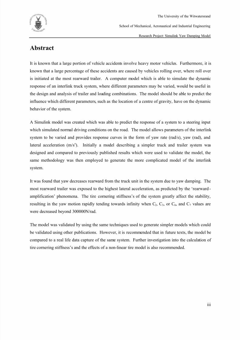
It is known that a large portion of vehicle accidents involve heavy motor vehicles. Furthermore, it is
known that a large percentage of these accidents are caused by vehicles rolling over, where roll over
is initiated at the most rearward trailer. A computer model which is able to simulate the dynamic
response of an interlink truck system, where different parameters may be varied, would be useful in
the design and analysis of trailer and loading combinations. The model should be able to predict the
influence which different parameters, such as the location of a centre of gravity, have on the dynamic
behavior of the system.
A Simulink model was created which was able to predict the response of a system to a steering input
which simulated normal driving conditions on the road. The model allows parameters of the interlink
system to be varied and provides response curves in the form of yaw rate (rad/s), yaw (rad), and
lateral acceleration (m/ss). Initially a model describing a simpler truck and trailer system was
designed and compared to previously published results which were used to validate the model, the
same methodology was then employed to generate the more complicated model of the interlink
system.
It was found that yaw decreases rearward from the truck unit in the system due to yaw damping. The
most rearward trailer was exposed to the highest lateral acceleration, as predicted by the ‘rearward -
amplification’ phenomena. The tir e cornering stiffness’s of the system greatly affect the stability,
resulting in the yaw motion rapidly tending towards infinity when C2, C3, or C6, and C7 values are
were decreased beyond 300000N/rad.
The model was validated by using the same techniques used to generate simpler models which could
be validated using other publications. However, it is recommended that in future texts, the model be
compared to a real life data capture of the same system. Further investigation into the calculation of
tire cornering stiffness’s and the effects of a non-linear tire model is also recommended.
8/13/2019 Simulink Yaw damping model
http://slidepdf.com/reader/full/simulink-yaw-damping-model 4/71
The University of the Witwatersrand
School of Mechanical, Aeronautical and Industrial Engineering
Research Project: Simulink Yaw Damping Model
iv
Table of Contents
Declaration .............................................................................................................................................. ii
Abstract .................................................................................................................................................. iii
Table of Contents ................................................................................................................................... iv
List of Figures ....................................................................................................................................... vii
List of Tables .......................................................................................................................................... x
1 Introduction .................................................................................................................................... 1
1.1 Motivation for Research.......................................................................................................... 1
2 Objectives ....................................................................................................................................... 3
3 Literature Review ........................................................................................................................... 4
3.1 Dynamic yaw response ........................................................................................................... 4
3.2 Two degree-of-freedom model ............................................................................................... 4
3.3 Understeer gradient ................................................................................................................. 5
3.4 Transfer functions ................................................................................................................... 5
3.5 Stability analysis ..................................................................................................................... 5
3.6 Tire cornering stiffness ........................................................................................................... 6
3.7 Stability ................................................................................................................................... 6
3.7.1 Root-locus plots .............................................................................................................. 6
3.7.2 Bode plots ....................................................................................................................... 6
8/13/2019 Simulink Yaw damping model
http://slidepdf.com/reader/full/simulink-yaw-damping-model 5/71
The University of the Witwatersrand
School of Mechanical, Aeronautical and Industrial Engineering
Research Project: Simulink Yaw Damping Model
v
3.7.3 Nyquist plots ................................................................................................................... 6
4 Analysis .......................................................................................................................................... 7
4.1 Single Vehicle Yaw Simulink Model ..................................................................................... 7
4.1.1 Assumptions .................................................................................................................... 7
4.1.2 Bicycle Model ................................................................................................................. 8
4.1.3 Equations of motion ........................................................................................................ 9
4.1.4 Simulink model ............................................................................................................... 9
4.2 Truck and trailer yaw simulink model .................................................................................. 10
4.2.1 Assumptions .................................................................................................................. 10
4.2.2 Bicycle model ............................................................................................................... 11
4.2.3 Equations of motion ...................................................................................................... 12
4.2.4 Simulink simulation model of truck and trailer system ................................................ 13
5 Experimentation ........................................................................................................................... 17
5.1 Assumptions .......................................................................................................................... 17
5.2 Bicycle model ....................................................................................................................... 18
5.3 Equations of motion .............................................................................................................. 20
5.4 Simulink model ..................................................................................................................... 24
5.5 Linear simulation of model ................................................................................................... 26
5.5.1 Parameters ..................................................................................................................... 26
5.5.2 Simulation results .......................................................................................................... 27
8/13/2019 Simulink Yaw damping model
http://slidepdf.com/reader/full/simulink-yaw-damping-model 6/71
The University of the Witwatersrand
School of Mechanical, Aeronautical and Industrial Engineering
Research Project: Simulink Yaw Damping Model
vi
5.6 Simulink model optimization ................................................................................................ 38
5.6.1 State space simulink model ........................................................................................... 38
5.6.2 Transfer function simulink model ................................................................................. 40
5.7 Stability ................................................................................................................................. 41
6 Discussion .................................................................................................................................... 47
7 Conclusion and Recommendations .............................................................................................. 53
8 Bibliography ................................................................................................................................. 55
9 References .................................................................................................................................... 56
Appendix A ........................................................................................................................................... 57
A.1 Derivation of equations of motion of one vehicle model ...................................................... 57
A.2 Derivation of equations of motion of truck and trailer model............................................... 58
Appendix B ........................................................................................................................................... 61
8/13/2019 Simulink Yaw damping model
http://slidepdf.com/reader/full/simulink-yaw-damping-model 7/71
The University of the Witwatersrand
School of Mechanical, Aeronautical and Industrial Engineering
Research Project: Simulink Yaw Damping Model
vii
List of Figures
Figure 1: Bicycle model [1] .................................................................................................................... 4
Figure 2: Single vehicle system .............................................................................................................. 7
Figure 3: 2-D.O.F. Bicycle model of single vehicle ............................................................................... 8
Figure 4: Yaw rate response of single vehicle system to chirp input .................................................... 10
Figure 5: Truck and trailer system ........................................................................................................ 10
Figure 6: Bicycle model of truck and trailer system ............................................................................. 11
Figure 7: Truck and trailer system vehicle lateral velocity response to sinusoidal input ..................... 14
Figure 8: Truck and trailer system vehicle yaw rate response to sinusoidal input ................................ 14
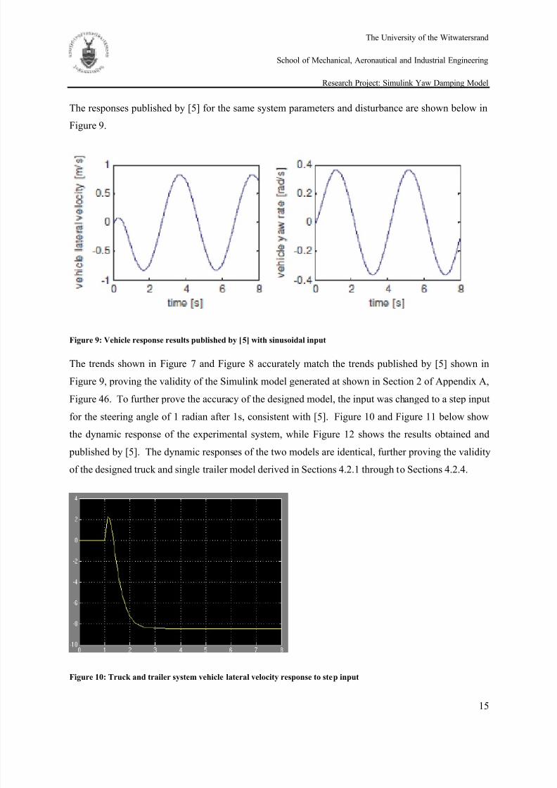
Figure 9: Vehicle response results published by [5] with sinusoidal input ........................................... 15
Figure 10: Truck and trailer system vehicle lateral velocity response to step input ............................. 15
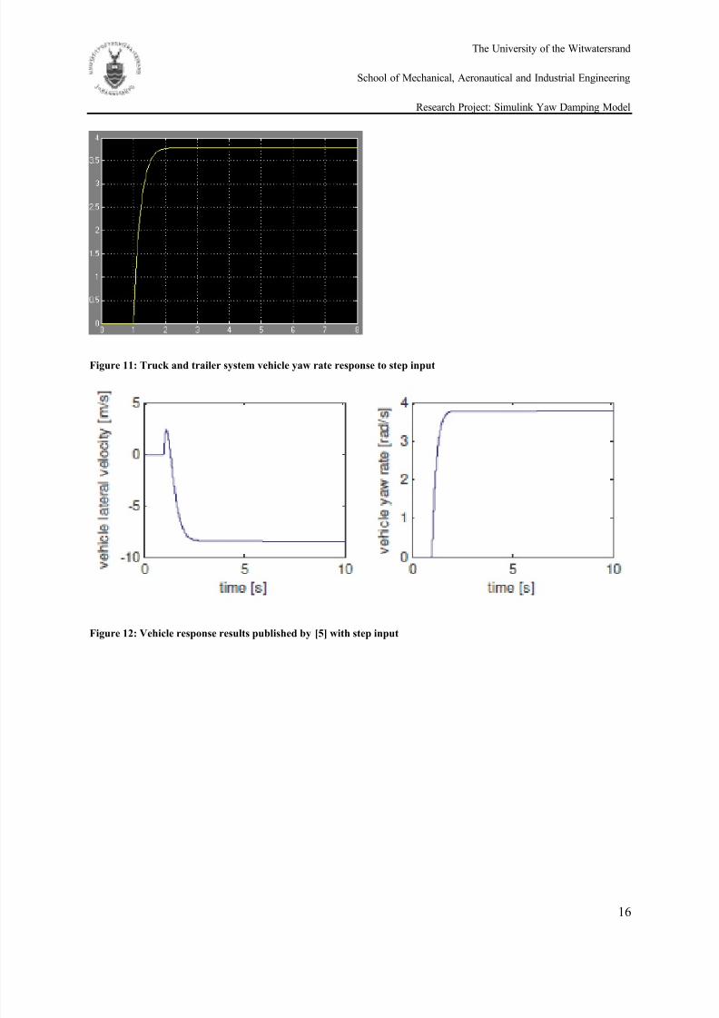
Figure 11: Truck and trailer system vehicle yaw rate response to step input ....................................... 16
Figure 12: Vehicle response results published by [5] with step input .................................................. 16
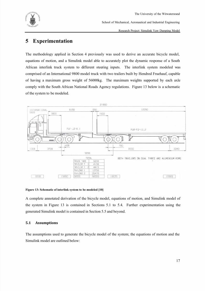
Figure 13: Schematic of interlink system to be modelled [10] ............................................................. 17
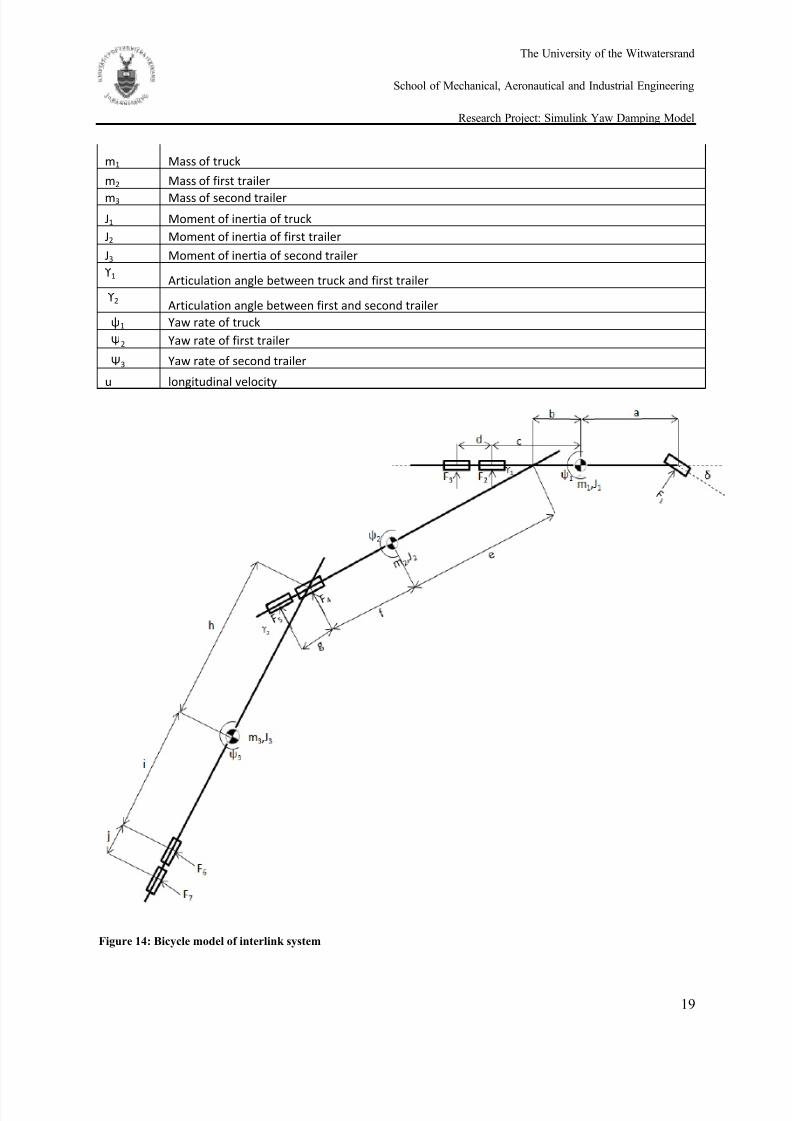
Figure 14: Bicycle model of interlink system ....................................................................................... 19
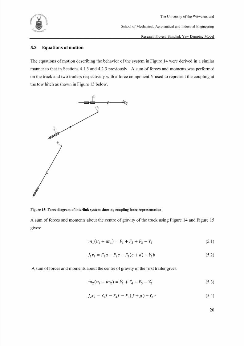
Figure 15: Force diagram of interlink system showing coupling force representation ......................... 20
Figure 16: Simulink model of interlink system .................................................................................... 25
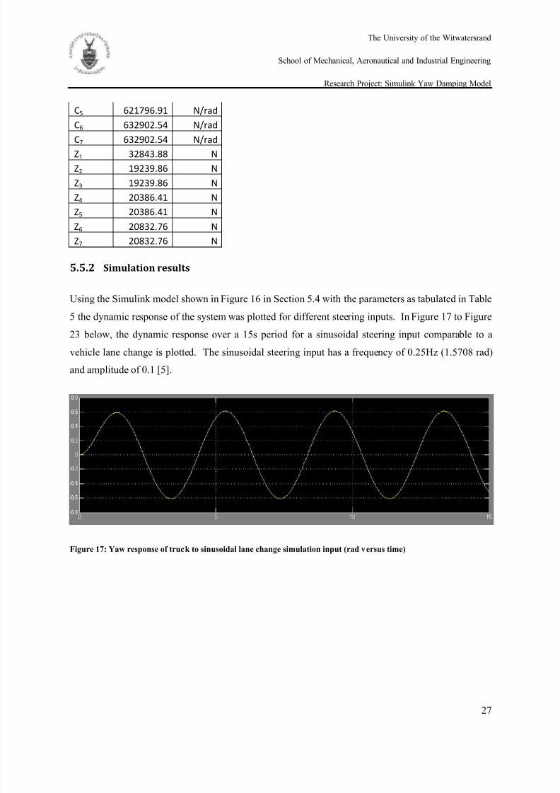
Figure 17: Yaw response of truck to sinusoidal lane change simulation input (rad versus time) ......... 27
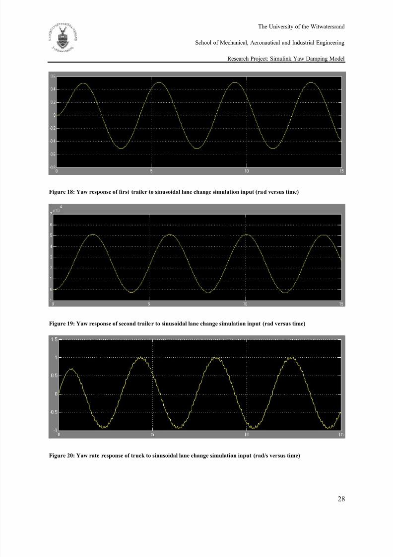
Figure 18: Yaw response of first trailer to sinusoidal lane change simulation input (rad versus time) 28
8/13/2019 Simulink Yaw damping model
http://slidepdf.com/reader/full/simulink-yaw-damping-model 8/71
The University of the Witwatersrand
School of Mechanical, Aeronautical and Industrial Engineering
Research Project: Simulink Yaw Damping Model
viii
Figure 19: Yaw response of second trailer to sinusoidal lane change simulation input (rad versus time)
.............................................................................................................................................................. 28
Figure 20: Yaw rate response of truck to sinusoidal lane change simulation input (rad/s versus time) 28
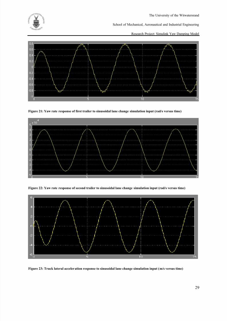
Figure 21: Yaw rate response of first trailer to sinusoidal lane change simulation input (rad/s versus
time) ...................................................................................................................................................... 29
Figure 22: Yaw rate response of second trailer to sinusoidal lane change simulation input (rad/s versus
time) ...................................................................................................................................................... 29
Figure 23: Truck lateral acceleration response to sinusoidal lane change simulation input (m/s versus
time) ...................................................................................................................................................... 29
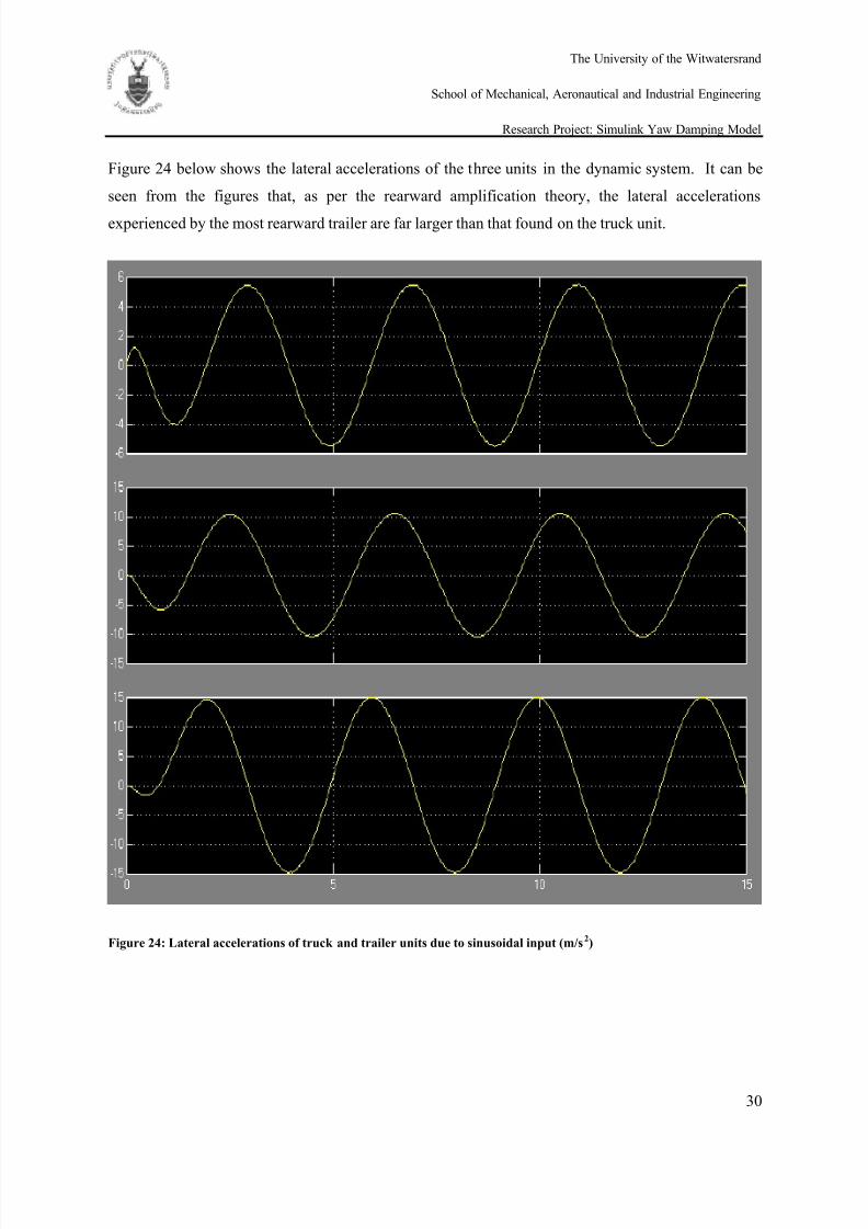
Figure 24: Lateral accelerations of truck and trailer units due to sinusoidal input (m/s2)..................... 30
Figure 25: System yaw response to chirp input .................................................................................... 31
Figure 26: System yaw rate response to sinusoidal input with first and second trailers same length
(rad/s) .................................................................................................................................................... 32
Figure 27: System yaw response to sinusoidal input with first and second trailers same length (rad) . 33
Figure 28: System lateral acceleration response to sinusoidal input with first and second trailers same
length (m/s2) .......................................................................................................................................... 33
Figure 29: System yaw rate response to sinusoidal input with first and second trailers swapped (rad/s)
.............................................................................................................................................................. 34
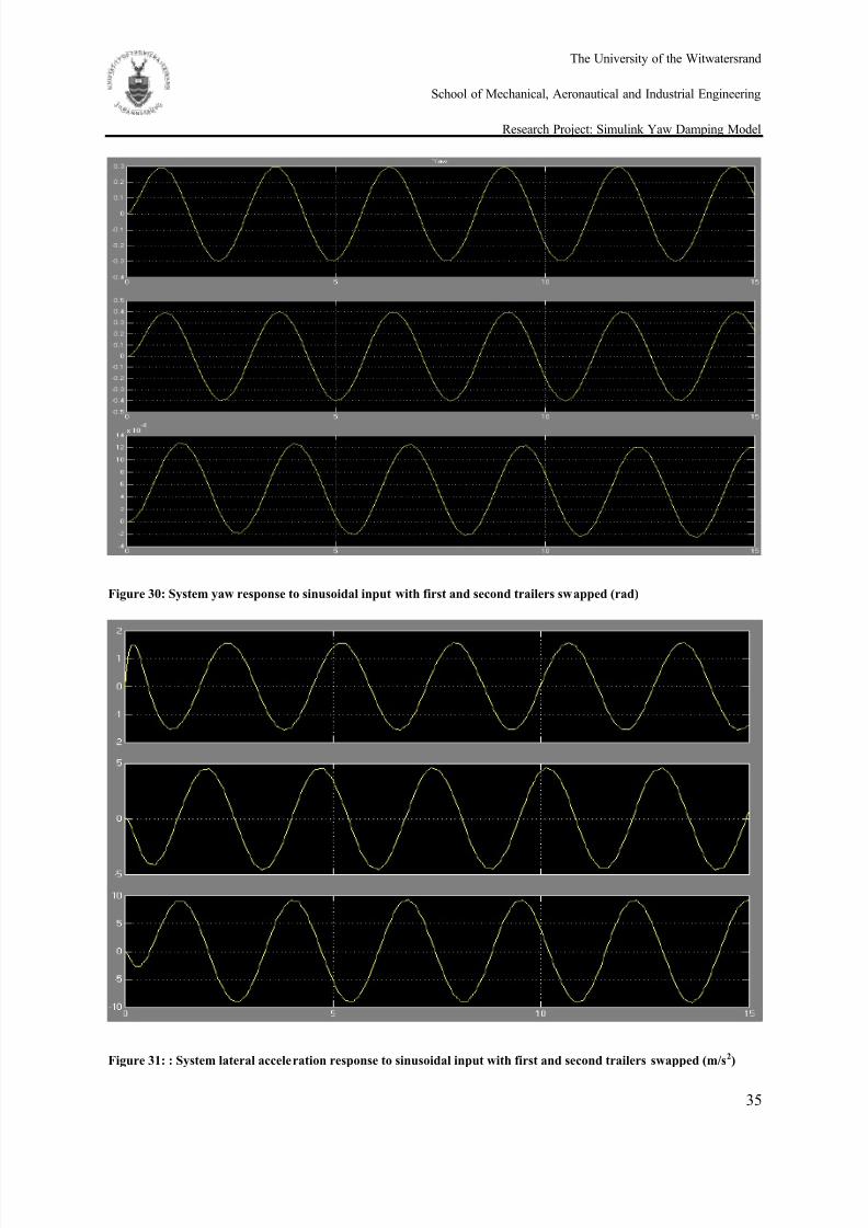
Figure 30: System yaw response to sinusoidal input with first and second trailers swapped (rad) ...... 35
Figure 31: : System lateral acceleration response to sinusoidal input with first and second trailers
swapped (m/s2) ...................................................................................................................................... 35
Figure 32: System yaw rate response to sinusoidal input with 25% original tire stiffnesses (rad/s) .... 36
Figure 33: System yaw response to sinusoidal input with 25% original tire stiffnesses (rad) .............. 37
8/13/2019 Simulink Yaw damping model
http://slidepdf.com/reader/full/simulink-yaw-damping-model 9/71
The University of the Witwatersrand
School of Mechanical, Aeronautical and Industrial Engineering
Research Project: Simulink Yaw Damping Model
ix
Figure 34: System yaw rate response to sinusoidal input with longitudinal velocity of 34m/s (rad/s) . 37
Figure 35: System yaw response to sinusoidal input with longitudinal velocity of 34m/s (rad) .......... 38
Figure 36: State space representation of interlink model ...................................................................... 39
Figure 37: State space model truck lateral acceleration response to sinusoidal input .......................... 39
Figure 38: State space model truck yaw response to sinusoidal input .................................................. 40
Figure 39: State space model second trailer yaw response to sinusoidal input..................................... 40
Figure 40: Transfer function model truck lateral acceleration response to sinusoidal input ................ 41
Figure 41: Root-locus plot of unstable system due to smaller C2 and C3 values .................................. 43
Figure 42: Yaw response of unstable system due to smaller C2 and C3 values .................................... 43
Figure 43: Root-locus plot of unstable system due to smaller C6 and C7 values .................................. 44
Figure 44: Root locus plot of the unstable system due to further forward centre of gravity on first
trailer ..................................................................................................................................................... 45
Figure 45: Root-locus plot of stable system due to swapping of first and second trailer parameters ... 46
Figure 46: Simulink model of truck and trailer ..................................................................................... 60
8/13/2019 Simulink Yaw damping model
http://slidepdf.com/reader/full/simulink-yaw-damping-model 10/71
8/13/2019 Simulink Yaw damping model
http://slidepdf.com/reader/full/simulink-yaw-damping-model 11/71
The University of the Witwatersrand
School of Mechanical, Aeronautical and Industrial Engineering
Research Project: Simulink Yaw Damping Model
1
1 Introduction
1.1
Motivation for Research
The dynamic instability in articulated vehicles is the cause of about 30% of accidents involving heavy
motor vehicles (HMVs) in New Zealand [1]. Most of the accidents are a result of vehicles rolling
over which is known to occur from the most rearward trailer rolling first, which in turn rolls the entire
vehicle onto its side [1]. The rolling over of the vehicle is a result of the rearward amplification of the
lateral acceleration of the trailers as a result of the turning frequency generated by the driver in a lane
change or evasive maneuver.
Motor vehicle accidents, in general, cause a large number of fatalities world-wide. Furthermore,
instability in an interlink HMV system (truck towing two trailers) may result in up to 56 tones
traveling out of control on the worlds highways with the potential to kill hundreds of people. In
addition to the fatalities caused, the loads carried by many of the vehicles are hazardous and may
contaminate the environment as a direct result of an accident. Finally, the traffic jams caused by
HMV accidents affect the economy of the country.
The poor state of the South African railway service has resulted in a large increase in the use of trucks
as the form of transport from the harbors to inland cities such as Johannesburg. The road from
Johannesburg to Durban is well maintained but the topology is not conducive to safe traveling for
HMVs as the winding and sharp descents on passes such as Van Reenen’s pass promote large steering
inputs of a high, regular frequency which can be exceptionally dangerous in an unstable HMV system.
The demand increase for trucks in South Africa has resulted in many new, inexperienced operators
taking to the road to take advantage of the market trend, however, the lack of experience and
knowledge of these operators could have catastrophic implications on the number of road accidents in
the country. The payload of a system is the mass of the load that the truck transports which the
supplier pays for, therefore, a larger payload on a system produces a larger turnover for the operator
per load transported. Unfortunately, a lack of knowledge of system characteristics results in loads
being placed dangerously on trailers and, although the policing of axle weights and loads is quite good
in the form of weigh bridges on all major traffic routes, the systems can be bypassed, and operators
are doing so, endangering the lives of all road users.
A simulation model where vehicle parameters can easily be changed to determine their influence on a
HMV system would be advantageous when designing a system or determining the best configuration
8/13/2019 Simulink Yaw damping model
http://slidepdf.com/reader/full/simulink-yaw-damping-model 12/71
The University of the Witwatersrand
School of Mechanical, Aeronautical and Industrial Engineering
Research Project: Simulink Yaw Damping Model
2
for a system in operation. Operators could use the model to understand the effects of the loadings on
the trailers and optimize their systems to attain the safest and most economical configuration for
themselves individually.
8/13/2019 Simulink Yaw damping model
http://slidepdf.com/reader/full/simulink-yaw-damping-model 13/71
The University of the Witwatersrand
School of Mechanical, Aeronautical and Industrial Engineering
Research Project: Simulink Yaw Damping Model
3
2 Objectives
Develop a simplified force model of an interlink South African truck and trailer system with
valid assumptions for force and impulse analysis:
o Constant friction on the tires
o No delay of input force
o The road surface is flat and level
o No aerodynamic forces influence the system
From the model, generate a model using Simulink to generate response curves relative to the
input frequency (steering):o Yaw rate and angle versus time
o Vehicle lateral acceleration versus time
Determine the yaw damping ratio of the system
Evaluate the influence of different vehicle parameters on the yaw motion of the system:
o Position and magnitude of centre of gravity of load
o Tire stiffness of vehicle
o Length of trailers
o Longitudinal velocity of vehicle
Make comparisons to other yaw damping models
8/13/2019 Simulink Yaw damping model
http://slidepdf.com/reader/full/simulink-yaw-damping-model 14/71
The University of the Witwatersrand
School of Mechanical, Aeronautical and Industrial Engineering
Research Project: Simulink Yaw Damping Model
4
3 Literature Review
3.1
Dynamic yaw response
A property that dominates the performance of the dynamic yaw response of a multi-articulated vehicle
is that known as rearward amplification. Other studies have found that during a transient turning
maneuver, the rear unit of the HMV may experience lateral accelerations far greater than that
experienced by the towing unit. The rearward amplification described is believed to be the property
which leads HMVs to roll from the rear trailer first. [3]
Rearward amplification is a frequency-sensitive phenomenon and seems to be more prominent when
the steering input has a high frequency. Multi articulated HMVs are multi-degree-of-freedom systems
with several lightly damped dynamic modes of oscillation and system excitement, due to evasive
maneuvers, in close proximity to these natural frequencies will cause an uncontrolled resonant
response. [4]
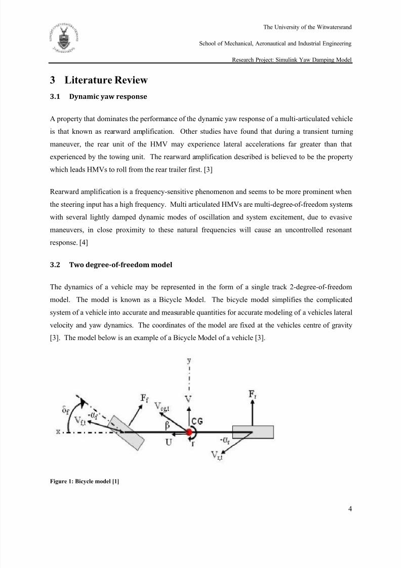
3.2 Two degree-of-freedom model
The dynamics of a vehicle may be represented in the form of a single track 2-degree-of-freedom
model. The model is known as a Bicycle Model. The bicycle model simplifies the complicated
system of a vehicle into accurate and measurable quantities for accurate modeling of a vehicles lateral
velocity and yaw dynamics. The coordinates of the model are fixed at the vehicles centre of gravity
[3]. The model below is an example of a Bicycle Model of a vehicle [3].
Figure 1: Bicycle model [1]
8/13/2019 Simulink Yaw damping model
http://slidepdf.com/reader/full/simulink-yaw-damping-model 15/71
The University of the Witwatersrand
School of Mechanical, Aeronautical and Industrial Engineering
Research Project: Simulink Yaw Damping Model
5
3.3 Understeer gradient
The understeer gradient is used to relate a vehicles weight distribution to its tires’ force generating
abilities. The understeer gradient is determined by modeling the bicycle model during a high speed
steady state turn and performing a sum of the forces and moments acting on the model. A vehicle
with a positive understeer gradient is known as an understeer vehicle and requires an increase in
steering input to negotiate a steady state turn as the speed of the vehicle increases. A vehicle with a
negative understeer gradient is known as an oversteer vehicle and the converse applies to that of an
understeer vehicle. [3]
3.4 Transfer functions
A multiply articulated vehicle is dynamically decoupled at the tow hitch if; for trains with more than
one full trailer results are consistent in that the two modes associated with a given full trailer tend to
be lightly damped and the addition of more trailers does not affect the dynamic behavior of units
ahead of the added trailers and the modes of motion associated with each full trailer become less and
less damped moving rearward. [4] The decoupling phenomenon allows each trailer unit to be
analyzed individually. The overall transfer function can be determined by multiplying the localized
transfer functions between centers of gravity and tow points along the length of the system in thisdecoupled system. [4]
3.5 Stability analysis
The state space form of the system can be used to calculate the stability parameters of the system.
The natural frequency of the undamped system (ωo), the natural frequency (ωn) and the damping ratio
(ξ) can be computed with use of the eigenvalues (λ ) of matrix A due to the time-independence of the
system matrices- forward velocity and tire cornering stiffness assumed constant. The parameters
necessary for a stability analysis can be calculated using Equations 3.1, 3.2, and 3.3 below [5]:
√ (3.1)
(3.2)
√ (3.3)
8/13/2019 Simulink Yaw damping model
http://slidepdf.com/reader/full/simulink-yaw-damping-model 16/71
The University of the Witwatersrand
School of Mechanical, Aeronautical and Industrial Engineering
Research Project: Simulink Yaw Damping Model
6
3.6 Tire cornering stiffness
The tire reactant force from the tire can be approximated to be a linear force with reference to the
stiffness coefficient of the tire, and the slip angle [4 – 9]. The tire cornering stiffness can be
approximated by Equation 3.4 below [8, 9]:
(3.4)
Where is the vertical load on the tire in Newtons [8, 9].
3.7 Stability
Linear systems are deemed to be unstable if either the real part of any one pole is positive, or any one
repeated pole has zero real parts, otherwise it is stable. Furthermore, a stable linear system having all
poles with negative real parts is asymptotically stable. [11]
3.7.1 Root-locus plots
Root-locus plots are used to plot the system roots over the range of a variable to determine if the
system becomes unstable. Positive real parts of roots will result in terms that grow exponentially and
become unstable while complex roots make a system oscillate. [12]
3.7.2 Bode plots
Bode plots are a useful way to represent the gain and phase of a system as a function of frequency,
known as the frequency-domain behavior of a system. The frequency response is shown with two
plots; one for magnitude, and one for phase. The phasor representation of the transfer function can be
easily determined at any frequency. The magnitude of the output is the magnitude of the phasor
representation of the transfer function (at a given frequency) multiplied by the magnitude of the input.
The phase of the output is the phase of the transfer function added to the phase of the input. [13]
3.7.3 Nyquist plots
Nyquist plots display both amplitude and phase angle on a single plot, using frequency as a parameter
in the plot. It is a polar plot of the frequency response of a system. [14]
8/13/2019 Simulink Yaw damping model
http://slidepdf.com/reader/full/simulink-yaw-damping-model 17/71
The University of the Witwatersrand
School of Mechanical, Aeronautical and Industrial Engineering
Research Project: Simulink Yaw Damping Model
7
4 Analysis
Yaw damping models describing the yaw motion of vehicle systems are available for different vehicle
system configurations in other research papers. Simulink models were initially created for a 1-vehicle
system followed by a truck and trailer system with the same properties as described in [3] and [5]
respectively and comparisons were made between the new Simulink model results and the results
published by [3] and [5] in order to validate the modeling method. The techniques used to build the
validated models described in Sections 4.1 and 4.2 below were used to generate a model describing
the behavior of an interlink South African truck system, discussed in Section 5.
4.1 Single Vehicle Yaw Simulink Model
A Simulink model describing the yaw characteristics of a single vehicle system was developed with
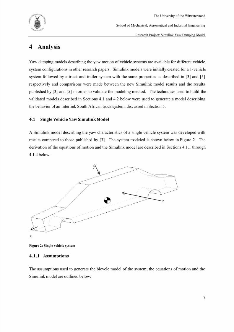
results compared to those published by [3]. The system modeled is shown below in Figure 2. The
derivation of the equations of motion and the Simulink model are described in Sections 4.1.1 through
4.1.4 below.
Figure 2: Single vehicle system
4.1.1 Assumptions
The assumptions used to generate the bicycle model of the system; the equations of motion and the
Simulink model are outlined below:
y
z
x
8/13/2019 Simulink Yaw damping model
http://slidepdf.com/reader/full/simulink-yaw-damping-model 18/71
The University of the Witwatersrand
School of Mechanical, Aeronautical and Industrial Engineering
Research Project: Simulink Yaw Damping Model
8
Vehicle mass and tire forces are symmetric about the x-z plane. Therefore, the vehicle can be
modelled as a single tracked vehicle where two front and two rear wheels can be represented
together as a single front and single rear wheel.
Longitudinal velocity is constant.
Tires roll without slipping in the longitudinal direction (no acceleration or braking forces).
Front and rear tires produce lateral forces which are linearly proportional to their respective
cornering stiffness’s (linear tire model).
Small angle approximations are valid: cosθ≈1, sinθ≈0.
4.1.2 Bicycle Model
The planar dynamics modeling of the vehicle were represented in the form of a single track, two-
degree of freedom model known as a ‘bicycle model’, consistent with the assumptions outlined in
Section 4.1.1 above. The bicycle model is an accurate model of the vehicles lateral velocity and yaw
dynamics and is described by a body-fixed coordinate system centered at the centre of gravity of the
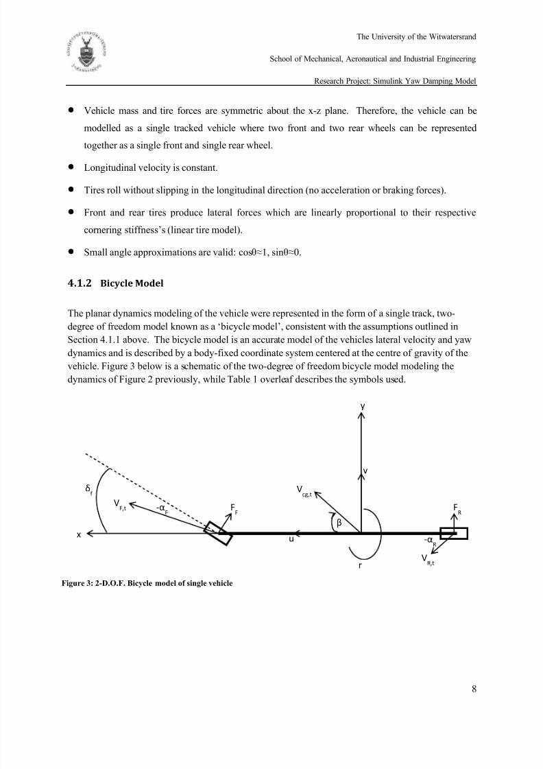
vehicle. Figure 3 below is a schematic of the two-degree of freedom bicycle model modeling the
dynamics of Figure 2 previously, while Table 1 overleaf describes the symbols used.
δf
y
Vcg,t
u
v
FR
VR,t
-αR x
VF,t
-αF
β
FF
r
Figure 3: 2-D.O.F. Bicycle model of single vehicle
8/13/2019 Simulink Yaw damping model
http://slidepdf.com/reader/full/simulink-yaw-damping-model 19/71
The University of the Witwatersrand
School of Mechanical, Aeronautical and Industrial Engineering
Research Project: Simulink Yaw Damping Model
9
Table 1: Single vehicle list of symbols
Symbol Description
Vcg,t
Total velocity vector at centre of gravity
u Longitudinal velocity
v Lateral velocity
r Yaw about z-axis
β Side slip angle
δf Front wheel steering angle
αF Front wheel slip angle
VF,t
Total velocity vector at front tire
FF Lateral force generated at front tire
αR Rear tire slip angle
VR,t
Total velocity vector at rear tire
FR Lateral force generated at rear tire
4.1.3 Equations of motion
The full derivation of the equations of motion of the one-vehicle system is shown in Section 1 of
Appendix A. Meaningful expressions of the equations are listed below in Equations X and Y.
(4.1) (4.2)
The standard state matrix representation of the equations is shown below:
[
]
4.1.4 Simulink model
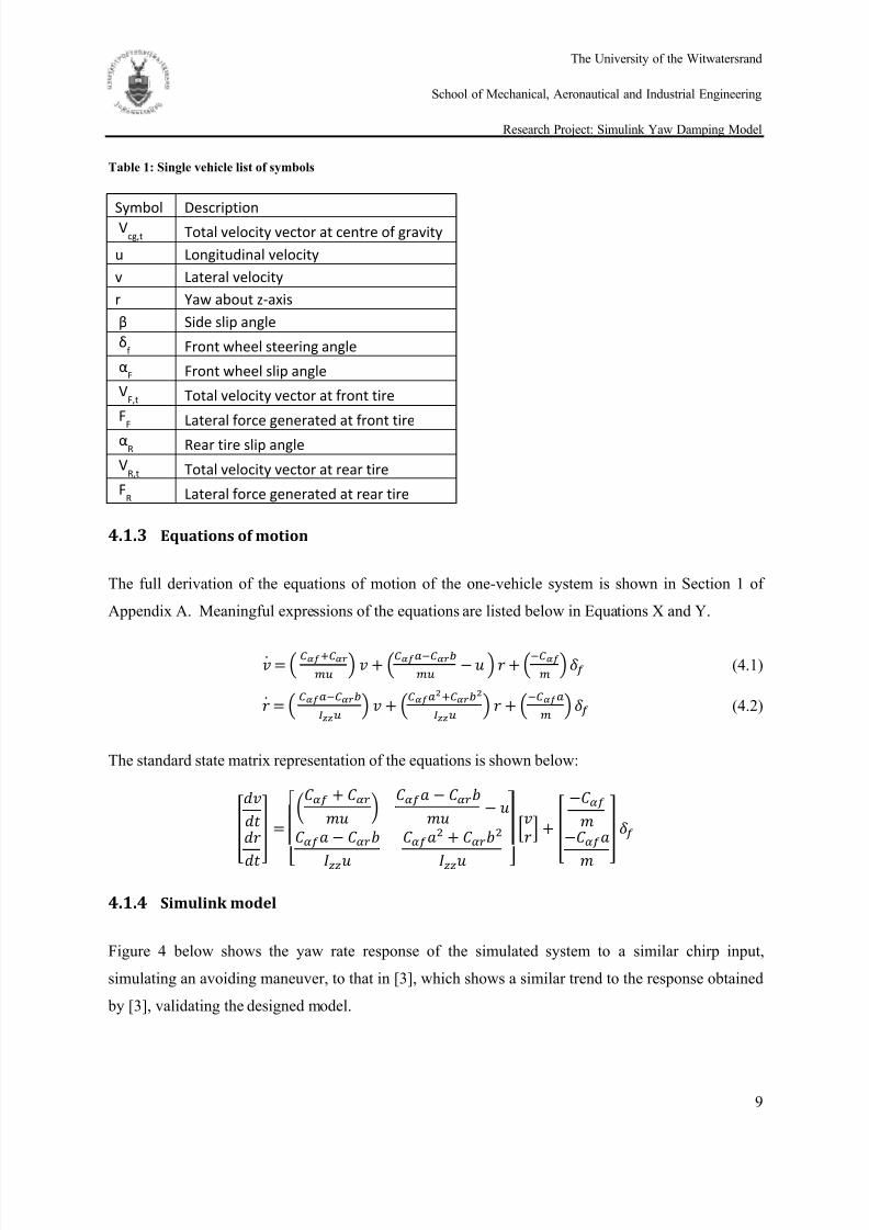
Figure 4 below shows the yaw rate response of the simulated system to a similar chirp input,
simulating an avoiding maneuver, to that in [3], which shows a similar trend to the response obtained
by [3], validating the designed model.
8/13/2019 Simulink Yaw damping model
http://slidepdf.com/reader/full/simulink-yaw-damping-model 20/71
The University of the Witwatersrand
School of Mechanical, Aeronautical and Industrial Engineering
Research Project: Simulink Yaw Damping Model
10
Figure 4: Yaw rate response of single vehicle system to chirp input
4.2 Truck and trailer yaw simulink model
The methods used to create the single vehicle model described in Section 4.1, previously, were
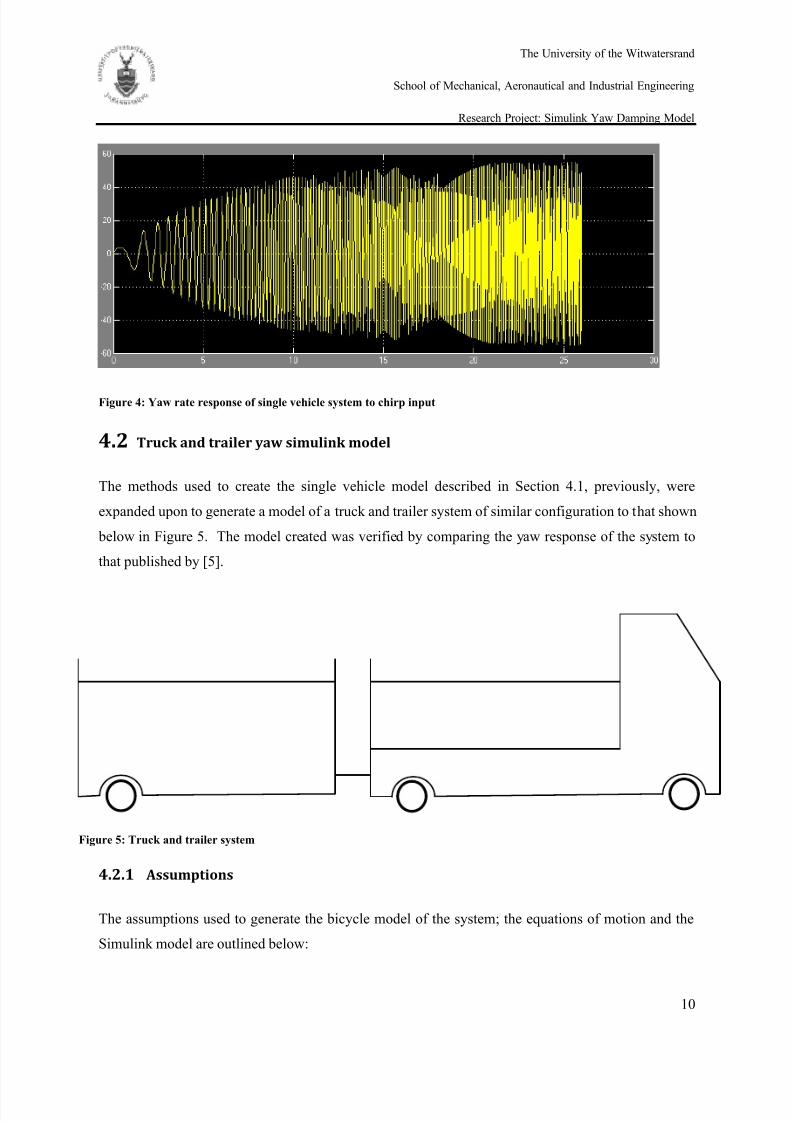
expanded upon to generate a model of a truck and trailer system of similar configuration to that shown
below in Figure 5. The model created was verified by comparing the yaw response of the system to
that published by [5].
4.2.1 Assumptions
The assumptions used to generate the bicycle model of the system; the equations of motion and the
Simulink model are outlined below:
Figure 5: Truck and trailer system
8/13/2019 Simulink Yaw damping model
http://slidepdf.com/reader/full/simulink-yaw-damping-model 21/71
The University of the Witwatersrand
School of Mechanical, Aeronautical and Industrial Engineering
Research Project: Simulink Yaw Damping Model
11
Vehicle mass and tire forces are symmetric about the x-z plane. Therefore, the vehicle can be
modelled as a single tracked vehicle where two front and two rear wheels can be represented
together as a single front and single rear wheel.
Longitudinal velocity is constant.
Tires roll without slipping in the longitudinal direction (no acceleration or braking forces).
Front and rear tires produce lateral forces which are linearly proportional to their respective
cornering stiffness’s (linear tire model).
The connection between the truck and trailer is solid (does not bend) and operates without
friction. Small angle approximations are valid: cosθ≈1, sinθ≈0.
4.2.2 Bicycle model
The assumptions outlined in Section 4.2.1 above were used to simplify the system described by Figure
5 into an accurate bicycle model describing the planar dynamic behavior of the coupled system.
Figure 6 below is a schematic of the bicycle model which was used to determine the equations of
motion of the system described in Section 4.2.3.
Figure 6: Bicycle model of truck and trailer system
Table 2 overleaf describes the symbols used and their description in the model and during the
derivation of the equations of motion in Section 4.2.3 below.
8/13/2019 Simulink Yaw damping model
http://slidepdf.com/reader/full/simulink-yaw-damping-model 22/71
The University of the Witwatersrand
School of Mechanical, Aeronautical and Industrial Engineering
Research Project: Simulink Yaw Damping Model
12
Table 2: Truck and trailer system list of symbols
Symbol Description
a Distance between the centre of gravity (C.O.G) of truck and the front steering wheel axle
b Distance between the C.O.G of the truck and the truck rear axle
c Distance between the C.O.G of the truck and the first tow hitch
d Distance between the C.O.G of the first trailer and the first tow hitch
e Distance between the C.O.G of the first trailer and the trailer axle
F1 Force generated by the front tires of the truck
F2 Force generated by the rear tires of the truck
F3 Force generated by the trailer tires
m1 Mass of the truckm2 Mass of the trailer
J1 Moment of inertia of the truck about its C.O.G
J2 Moment of inertia of the trailer about its centre of gravity
ψ Yaw angle of truck
ϒ Articulation angle
δ Steering angle
αi Tire side slip angle
Ci Tire cornering stiffness
4.2.3 Equations of motion
The full derivation of the equations of motion of the truck and trailer system is shown in Section 2 of
Appendix A. Meaningful expressions of the equations are listed below in Equations 4.3, 4.4 and 4.5.
(4.3)
(4.4)
() (4.5)
The linear tire model approximation was used to calculate the force components applied by each tire:
, (4.6)
where i=1, 2, 3, for each individual tire.
8/13/2019 Simulink Yaw damping model
http://slidepdf.com/reader/full/simulink-yaw-damping-model 23/71
The University of the Witwatersrand
School of Mechanical, Aeronautical and Industrial Engineering
Research Project: Simulink Yaw Damping Model
13
The matrix form of the system can be written in the form , where j is the input
(steering input), as shown below:
[
]
4.2.4 Simulink simulation model of truck and trailer system
A simulink model was generated to determine the vehicle behavior when subjected to a steering input
using the assumptions and equations of motion outlined in preceding sections. The input parameters
chosen for the simulation were taken from [5] in order to validate the modeling technique and
derivations performed. Table 3 below is taken from [5] and shows the parameters used in the
Simulink simulation.
Table 3: Truck and trailer simulink model vehicle parameters [5]
Parameter Unit Value
a m 2.062
b m 2.723
c m 2.539
d m 7.483
e m 3.76
C1 N/rad 381930C2 N/rad 733390
C3 N/rad 881440
m1 kg 8812
m2 kg 16484
J1 kg.m2 46100
J2 kg.m2 452010
A schematic of the Simulink model designed is contained in Section 2 of Appendix A in Figure 46.
8/13/2019 Simulink Yaw damping model
http://slidepdf.com/reader/full/simulink-yaw-damping-model 24/71
The University of the Witwatersrand
School of Mechanical, Aeronautical and Industrial Engineering
Research Project: Simulink Yaw Damping Model
14
A sinusoidal steering input with a frequency of 0.25 Hz and amplitude 0.1 radians to simulate a lane
change was applied as the steering input, consistent with the values used by [5], furthermore, a
longitudinal velocity component (u) was selected to be 20m/s. The dynamic response of the system
was plotted using scopes in the Simulink environment. The vehicle lateral velocity (m/s) and vehicle
yaw rate (rad/s) dynamic responses over an 8s simulation period are shown below in Figure 7 and
Figure 8 respectively.
Figure 7: Truck and trailer system vehicle lateral velocity response to sinusoidal input
Figure 8: Truck and trailer system vehicle yaw rate response to sinusoidal input
8/13/2019 Simulink Yaw damping model
http://slidepdf.com/reader/full/simulink-yaw-damping-model 25/71
The University of the Witwatersrand
School of Mechanical, Aeronautical and Industrial Engineering
Research Project: Simulink Yaw Damping Model
15
The responses published by [5] for the same system parameters and disturbance are shown below in
Figure 9.
Figure 9: Vehicle response results published by [5] with sinusoidal input
The trends shown in Figure 7 and Figure 8 accurately match the trends published by [5] shown in
Figure 9, proving the validity of the Simulink model generated at shown in Section 2 of Appendix A,
Figure 46. To further prove the accuracy of the designed model, the input was changed to a step input
for the steering angle of 1 radian after 1s, consistent with [5]. Figure 10 and Figure 11 below show
the dynamic response of the experimental system, while Figure 12 shows the results obtained and
published by [5]. The dynamic responses of the two models are identical, further proving the validity
of the designed truck and single trailer model derived in Sections 4.2.1 through to Sections 4.2.4.
Figure 10: Truck and trailer system vehicle lateral velocity response to step input
8/13/2019 Simulink Yaw damping model
http://slidepdf.com/reader/full/simulink-yaw-damping-model 26/71
The University of the Witwatersrand
School of Mechanical, Aeronautical and Industrial Engineering
Research Project: Simulink Yaw Damping Model
16
Figure 11: Truck and trailer system vehicle yaw rate response to step input
Figure 12: Vehicle response results published by [5] with step input
8/13/2019 Simulink Yaw damping model
http://slidepdf.com/reader/full/simulink-yaw-damping-model 27/71
The University of the Witwatersrand
School of Mechanical, Aeronautical and Industrial Engineering
Research Project: Simulink Yaw Damping Model
17
5 Experimentation
The methodology applied in Section 4 previously was used to derive an accurate bicycle model,
equations of motion, and a Simulink model able to accurately plot the dynamic response of a South
African interlink truck system to different steering inputs. The interlink system modeled was
comprised of an International 9800 model truck with two trailers built by Hendred Fruehauf, capable
of having a maximum gross weight of 56000kg. The maximum weights supported by each axle
comply with the South African National Roads Agency regulations. Figure 13 below is a schematic
of the system to be modeled.
Figure 13: Schematic of interlink system to be modeled [10]
A complete annotated derivation of the bicycle model, equations of motion, and Simulink model of
the system in Figure 13 is contained in Sections 5.1 to 5.4. Further experimentation using the
generated Simulink model is contained in Section 5.5 and beyond.
5.1 Assumptions
The assumptions used to generate the bicycle model of the system; the equations of motion and the
Simulink model are outlined below:
8/13/2019 Simulink Yaw damping model
http://slidepdf.com/reader/full/simulink-yaw-damping-model 28/71
The University of the Witwatersrand
School of Mechanical, Aeronautical and Industrial Engineering
Research Project: Simulink Yaw Damping Model
18
Vehicle mass and tire forces are symmetric about the x-z plane. Therefore, the vehicle can be
modelled as a single tracked vehicle where two front and two rear wheels can be represented
together as a single front and single rear wheel.
Longitudinal velocity is constant.
Tires roll without slipping in the longitudinal direction (no acceleration or braking forces).
Front and rear tires produce lateral forces which are linearly proportional to their respective
cornering stiffness’s (linear tire model).
The connection between the truck and trailer is solid (does not bend) and operates without
friction. The centre of gravity location in the trailers can be approximated to be in the middle of the load.
i.e. the trailers are loaded symmetrically.
Small angle approximations are valid: cosθ≈1, sinθ≈0.
5.2 Bicycle model
The assumptions outlined in Section 5.1 above were used to simplify the system described by Figure
13 into an accurate bicycle model describing the planar dynamic behavior of the coupled system.
Figure 14 overleaf is a force diagram of the bicycle model which was used to determine the equations
of motion of the system described in Section 5.3, while Table 4: Description of symbols used in
interlink model is a nomenclature of the symbols used.
Table 4: Description of symbols used in interlink model
Symbol Description
a Distance between centre of gravity (C.O.G) of truck and front tire
b Distance between C.O.G of truck and first hitch point
c Distance between C.O.G of truck and first axle of truck
d Distance between first and second truck axles
e Distance between C.O.G of first trailer and first hitch point
f Distance between C.O.G of first trailer and second hitch point/first axle on first trailer
g Distance between first and second axles on first trailer
h Distance between C.O.G of second trailer and second hitch point
i Distance between C.O.G of second trailer and first axle on second trailer
j Distance between first and second axle on second trailer
Fi Force generated by tires
8/13/2019 Simulink Yaw damping model
http://slidepdf.com/reader/full/simulink-yaw-damping-model 29/71
The University of the Witwatersrand
School of Mechanical, Aeronautical and Industrial Engineering
Research Project: Simulink Yaw Damping Model
19
m1 Mass of truck
m2 Mass of first trailer
m3 Mass of second trailer
J1 Moment of inertia of truck
J2 Moment of inertia of first trailer
J3 Moment of inertia of second trailer
ϒ1 Articulation angle between truck and first trailer
ϒ2 Articulation angle between first and second trailer
ψ1 Yaw rate of truck
Ψ2 Yaw rate of first trailer
Ψ3 Yaw rate of second trailer
u longitudinal velocity
Figure 14: Bicycle model of interlink system
8/13/2019 Simulink Yaw damping model
http://slidepdf.com/reader/full/simulink-yaw-damping-model 30/71
8/13/2019 Simulink Yaw damping model
http://slidepdf.com/reader/full/simulink-yaw-damping-model 31/71
The University of the Witwatersrand
School of Mechanical, Aeronautical and Industrial Engineering
Research Project: Simulink Yaw Damping Model
21
A sum of forces and moments about the centre of gravity of the second trailer gives:
(5.5)
(5.6)
Solving for Y1 using Equation 5.2 and substituting into Equation 5.1:
(5.7)
Solving for Y2 using Equations 5.1 and 5.5 and substituting into Equation 5.3:
(5.8)
Equation 5.8 can be written in terms of the trucks C.O.G coordinate system using:
(5.9)
(5.10)
Substituting Equations 5.9 and 5.10 into 5.8:
( ) (5.11)
Further combinations of the above equations produce the final two equations of motion:
(5.12)
(5.13)
The reactant force generated in the tires was again approximated to be linear:
8/13/2019 Simulink Yaw damping model
http://slidepdf.com/reader/full/simulink-yaw-damping-model 32/71
The University of the Witwatersrand
School of Mechanical, Aeronautical and Industrial Engineering
Research Project: Simulink Yaw Damping Model
22
The slip angles for each tire are given by:
(5.14)
(5.15)
(5.16)
(5.17)
(5.18)
(5.19)
(5.20)
The articulation rates were calculated as follows:
(5.21)
(5.22)
The tire stiffness constant Ci was calculated using the following from [8, 9]:
(5.23)
where zi is the load supported by the tire.
As in Section 4.2.3, the equations can be represented in matrix form where:
M = bm1 I1 0 0 0 0
m1+m2+m3 -b(m2+m3) -f(m2+m3)-m3e m3h 0 0
fm1-em3 em3b m3e(f+e)+I2 m3eh 0 0
hm3 m3bh m3h(f+e) m3(h2)-I3 0 0
0 0 0 0 1 0
0 0 0 0 0 1
8/13/2019 Simulink Yaw damping model
http://slidepdf.com/reader/full/simulink-yaw-damping-model 33/71
The University of the Witwatersrand
School of Mechanical, Aeronautical and Industrial Engineering
Research Project: Simulink Yaw Damping Model
23
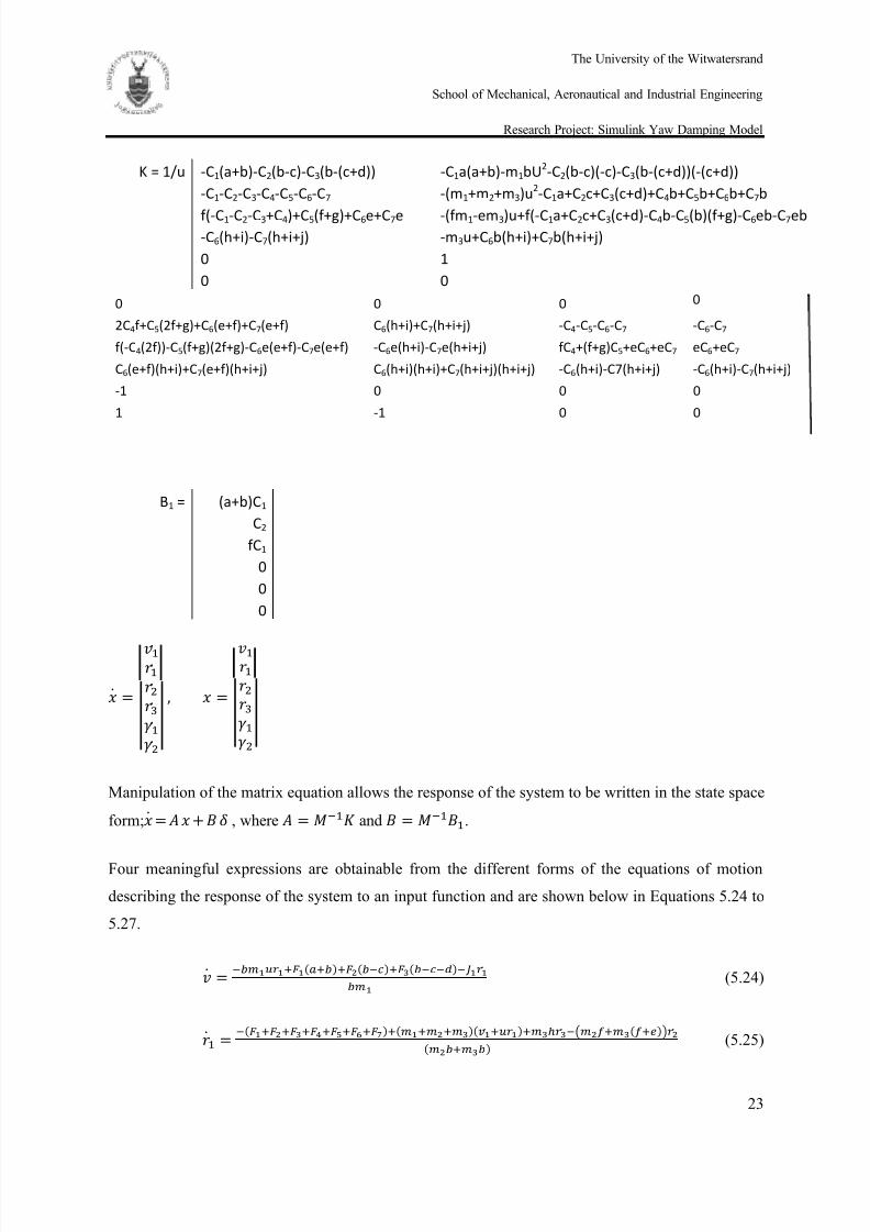
K = 1/u -C1(a+b)-C2(b-c)-C3(b-(c+d)) -C1a(a+b)-m1bU2-C2(b-c)(-c)-C3(b-(c+d))(-(c+d))
-C1-C2-C3-C4-C5-C6-C7 -(m1+m2+m3)u2-C1a+C2c+C3(c+d)+C4b+C5b+C6b+C7b
f(-C1-C2-C3+C4)+C5(f+g)+C6e+C7e -(fm1-em3)u+f(-C1a+C2c+C3(c+d)-C4b-C5(b)(f+g)-C6eb-C7eb-C6(h+i)-C7(h+i+j) -m3u+C6b(h+i)+C7b(h+i+j)
0 1
0 0
0 0 0 0
2C4f+C5(2f+g)+C6(e+f)+C7(e+f) C6(h+i)+C7(h+i+j) -C4-C5-C6-C7 -C6-C7
f(-C4(2f))-C5(f+g)(2f+g)-C6e(e+f)-C7e(e+f) -C6e(h+i)-C7e(h+i+j) fC4+(f+g)C5+eC6+eC7 eC6+eC7
C6(e+f)(h+i)+C7(e+f)(h+i+j) C6(h+i)(h+i)+C7(h+i+j)(h+i+j) -C6(h+i)-C7(h+i+j) -C6(h+i)-C7(h+i+j)
-1 0 0 0
1 -1 0 0
B1 = (a+b)C1
C2
fC1
0
0
0
| | |
|
Manipulation of the matrix equation allows the response of the system to be written in the state space
form; , where and .
Four meaningful expressions are obtainable from the different forms of the equations of motion
describing the response of the system to an input function and are shown below in Equations 5.24 to
5.27.
(5.24)
() (5.25)
8/13/2019 Simulink Yaw damping model
http://slidepdf.com/reader/full/simulink-yaw-damping-model 34/71
The University of the Witwatersrand
School of Mechanical, Aeronautical and Industrial Engineering
Research Project: Simulink Yaw Damping Model
24
(5.26)
(5.27)
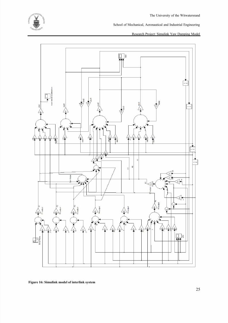
5.4 Simulink model
The equations of motion were used to build a Simulink model of the interlink system. The model was
designed to replicate the behavior of the real life system with given parameters in response to a
steering input over a time period. The Simulink model created is based on the idealized bicycle
model described in Section 5.2 and the derived equations of motion in Section 5.3 and is shown
overleaf in Figure 16.
8/13/2019 Simulink Yaw damping model
http://slidepdf.com/reader/full/simulink-yaw-damping-model 35/71
The University of the Witwatersrand
School of Mechanical, Aeronautical and Industrial Engineering
Research Project: Simulink Yaw Damping Model
25
Figure 16: Simulink model of interlink system
8/13/2019 Simulink Yaw damping model
http://slidepdf.com/reader/full/simulink-yaw-damping-model 36/71
The University of the Witwatersrand
School of Mechanical, Aeronautical and Industrial Engineering
Research Project: Simulink Yaw Damping Model
26
5.5 Linear simulation of model
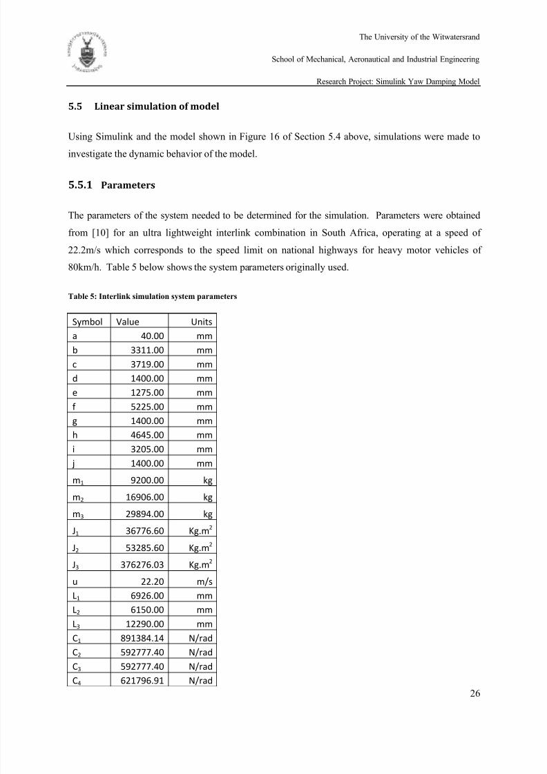
Using Simulink and the model shown in Figure 16 of Section 5.4 above, simulations were made to
investigate the dynamic behavior of the model.
5.5.1 Parameters
The parameters of the system needed to be determined for the simulation. Parameters were obtained
from [10] for an ultra lightweight interlink combination in South Africa, operating at a speed of
22.2m/s which corresponds to the speed limit on national highways for heavy motor vehicles of
80km/h. Table 5 below shows the system parameters originally used.
Table 5: Interlink simulation system parameters
Symbol Value Units
a 40.00 mm
b 3311.00 mm
c 3719.00 mm
d 1400.00 mm
e 1275.00 mm
f 5225.00 mmg 1400.00 mm
h 4645.00 mm
i 3205.00 mm
j 1400.00 mm
m1 9200.00 kg
m2 16906.00 kg
m3 29894.00 kg
J1 36776.60 Kg.m2
J2 53285.60 Kg.m2
J3 376276.03 Kg.m2
u 22.20 m/s
L1 6926.00 mm
L2 6150.00 mm
L3 12290.00 mm
C1 891384.14 N/rad
C2 592777.40 N/rad
C3 592777.40 N/rad
C4 621796.91 N/rad
8/13/2019 Simulink Yaw damping model
http://slidepdf.com/reader/full/simulink-yaw-damping-model 37/71
The University of the Witwatersrand
School of Mechanical, Aeronautical and Industrial Engineering
Research Project: Simulink Yaw Damping Model
27
C5 621796.91 N/rad
C6 632902.54 N/rad
C7 632902.54 N/radZ1 32843.88 N
Z2 19239.86 N
Z3 19239.86 N
Z4 20386.41 N
Z5 20386.41 N
Z6 20832.76 N
Z7 20832.76 N
5.5.2 Simulation results
Using the Simulink model shown in Figure 16 in Section 5.4 with the parameters as tabulated in Table
5 the dynamic response of the system was plotted for different steering inputs. In Figure 17 to Figure
23 below, the dynamic response over a 15s period for a sinusoidal steering input comparable to a
vehicle lane change is plotted. The sinusoidal steering input has a frequency of 0.25Hz (1.5708 rad)
and amplitude of 0.1 [5].
Figure 17: Yaw response of truck to sinusoidal lane change simulation input (rad versus time)
8/13/2019 Simulink Yaw damping model
http://slidepdf.com/reader/full/simulink-yaw-damping-model 38/71
8/13/2019 Simulink Yaw damping model
http://slidepdf.com/reader/full/simulink-yaw-damping-model 39/71
The University of the Witwatersrand
School of Mechanical, Aeronautical and Industrial Engineering
Research Project: Simulink Yaw Damping Model
29
Figure 21: Yaw rate response of first trailer to sinusoidal lane change simulation input (rad/s versus time)
Figure 22: Yaw rate response of second trailer to sinusoidal lane change simulation input (rad/s versus time)
Figure 23: Truck lateral acceleration response to sinusoidal lane change simulation input (m/s versus time)
8/13/2019 Simulink Yaw damping model
http://slidepdf.com/reader/full/simulink-yaw-damping-model 40/71
8/13/2019 Simulink Yaw damping model
http://slidepdf.com/reader/full/simulink-yaw-damping-model 41/71
The University of the Witwatersrand
School of Mechanical, Aeronautical and Industrial Engineering
Research Project: Simulink Yaw Damping Model
31
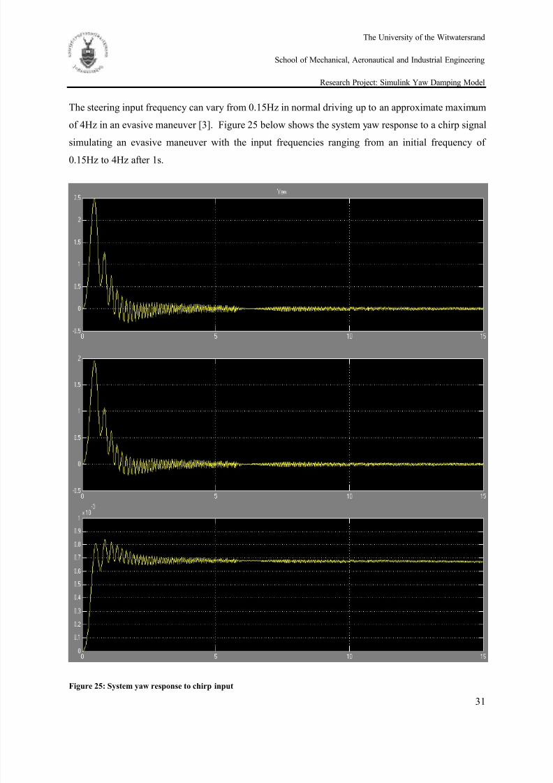
The steering input frequency can vary from 0.15Hz in normal driving up to an approximate maximum
of 4Hz in an evasive maneuver [3]. Figure 25 below shows the system yaw response to a chirp signal
simulating an evasive maneuver with the input frequencies ranging from an initial frequency of
0.15Hz to 4Hz after 1s.
Figure 25: System yaw response to chirp input
8/13/2019 Simulink Yaw damping model
http://slidepdf.com/reader/full/simulink-yaw-damping-model 42/71
8/13/2019 Simulink Yaw damping model
http://slidepdf.com/reader/full/simulink-yaw-damping-model 43/71
The University of the Witwatersrand
School of Mechanical, Aeronautical and Industrial Engineering
Research Project: Simulink Yaw Damping Model
33
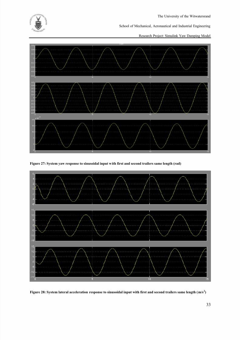
Figure 27: System yaw response to sinusoidal input with first and second trailers same length (rad)
Figure 28: System lateral acceleration response to sinusoidal input with first and second trailers same length (m/s2)
8/13/2019 Simulink Yaw damping model
http://slidepdf.com/reader/full/simulink-yaw-damping-model 44/71
The University of the Witwatersrand
School of Mechanical, Aeronautical and Industrial Engineering
Research Project: Simulink Yaw Damping Model
34
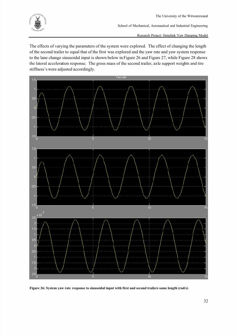
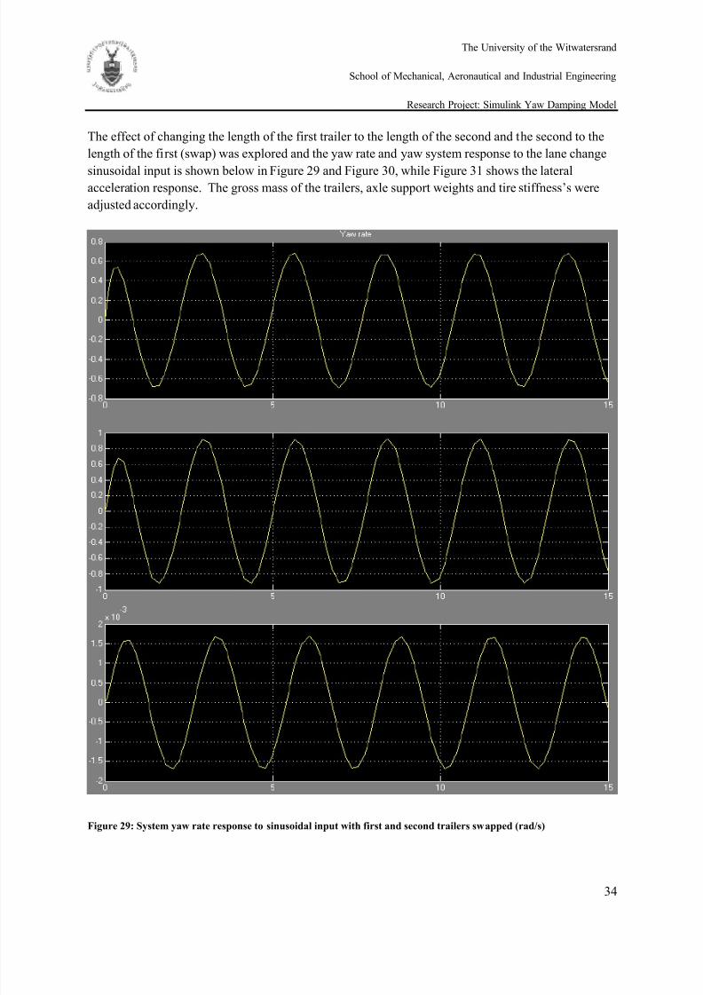
The effect of changing the length of the first trailer to the length of the second and the second to the
length of the first (swap) was explored and the yaw rate and yaw system response to the lane change
sinusoidal input is shown below in Figure 29 and Figure 30, while Figure 31 shows the lateralacceleration response. The gross mass of the trailers, axle support weights and tire stiffness’s were
adjusted accordingly.
Figure 29: System yaw rate response to sinusoidal input with first and second trailers swapped (rad/s)
8/13/2019 Simulink Yaw damping model
http://slidepdf.com/reader/full/simulink-yaw-damping-model 45/71
The University of the Witwatersrand
School of Mechanical, Aeronautical and Industrial Engineering
Research Project: Simulink Yaw Damping Model
35
Figure 30: System yaw response to sinusoidal input with first and second trailers swapped (rad)
Figure 31: : System lateral acceleration response to sinusoidal input with first and second trailers swapped (m/s2)
8/13/2019 Simulink Yaw damping model
http://slidepdf.com/reader/full/simulink-yaw-damping-model 46/71
The University of the Witwatersrand
School of Mechanical, Aeronautical and Industrial Engineering
Research Project: Simulink Yaw Damping Model
36
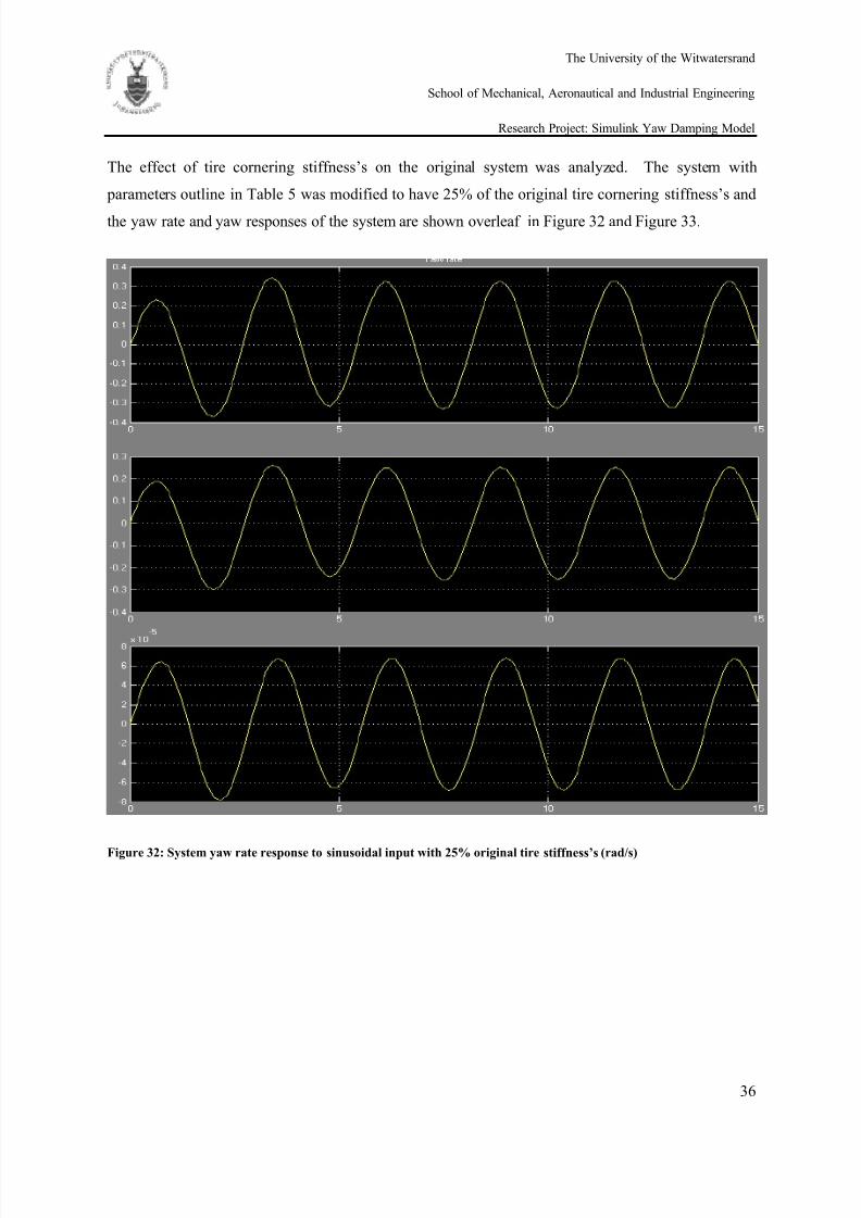
The effect of tire cornering stiffness’s on the original system was analyzed. The system with
parameters outline in Table 5 was modified to have 25% of the original tire cornering stiffness’s and
the yaw rate and yaw responses of the system are shown overleaf in Figure 32 and Figure 33.
Figure 32: System yaw rate response to sinusoidal input with 25% original tire stiffness’s (rad/s)
8/13/2019 Simulink Yaw damping model
http://slidepdf.com/reader/full/simulink-yaw-damping-model 47/71
The University of the Witwatersrand
School of Mechanical, Aeronautical and Industrial Engineering
Research Project: Simulink Yaw Damping Model
37
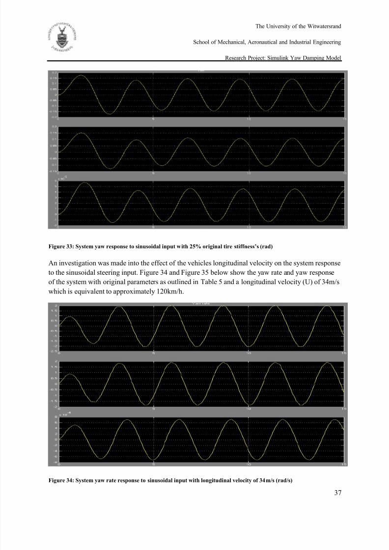
Figure 33: System yaw response to sinusoidal input with 25% original tire stiffness’s (rad)
An investigation was made into the effect of the vehicles longitudinal velocity on the system response
to the sinusoidal steering input. Figure 34 and Figure 35 below show the yaw rate and yaw response
of the system with original parameters as outlined in Table 5 and a longitudinal velocity (U) of 34m/s
which is equivalent to approximately 120km/h.
Figure 34: System yaw rate response to sinusoidal input with longitudinal velocity of 34m/s (rad/s)
8/13/2019 Simulink Yaw damping model
http://slidepdf.com/reader/full/simulink-yaw-damping-model 48/71
The University of the Witwatersrand
School of Mechanical, Aeronautical and Industrial Engineering
Research Project: Simulink Yaw Damping Model
38
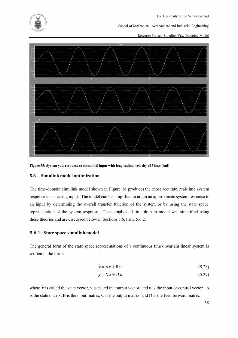
Figure 35: System yaw response to sinusoidal input with longitudinal velocity of 34m/s (rad)
5.6
Simulink model optimization
The time-domain simulink model shown in Figure 16 produces the most accurate, real-time system
response to a steering input. The model can be simplified to attain an approximate system response to
an input by determining the overall transfer function of the system or by using the state space
representation of the system response. The complicated time-domain model was simplified using
these theories and are discussed below in Sections 5.6.1 and 5.6.2.
5.6.1 State space simulink model
The general form of the state space representations of a continuous time-invariant linear system is
written in the form:
(5.28) (5.29)
where
is called the state vector, y is called the output vector, and u is the input or control vector. A
is the state matrix, B is the input matrix, C is the output matrix, and D is the feed forward matrix.
8/13/2019 Simulink Yaw damping model
http://slidepdf.com/reader/full/simulink-yaw-damping-model 49/71
The University of the Witwatersrand
School of Mechanical, Aeronautical and Industrial Engineering
Research Project: Simulink Yaw Damping Model
39
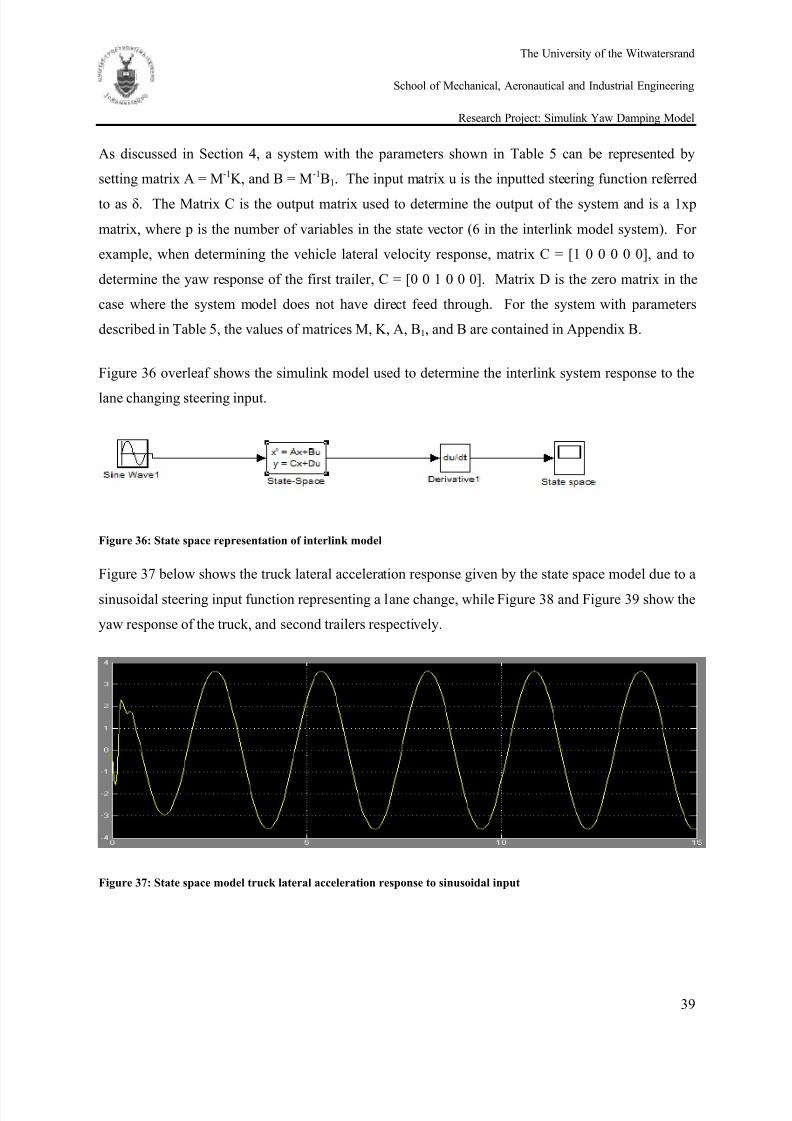
As discussed in Section 4, a system with the parameters shown in Table 5 can be represented by
setting matrix A = M-1K, and B = M-1B1. The input matrix u is the inputted steering function referred
to as δ. The Matrix C is the output matrix used to determine the output of the system and is a 1xp
matrix, where p is the number of variables in the state vector (6 in the interlink model system). For
example, when determining the vehicle lateral velocity response, matrix C = [1 0 0 0 0 0], and to
determine the yaw response of the first trailer, C = [0 0 1 0 0 0]. Matrix D is the zero matrix in the
case where the system model does not have direct feed through. For the system with parameters
described in Table 5, the values of matrices M, K, A, B1, and B are contained in Appendix B.
Figure 36 overleaf shows the simulink model used to determine the interlink system response to the
lane changing steering input.
Figure 36: State space representation of interlink model
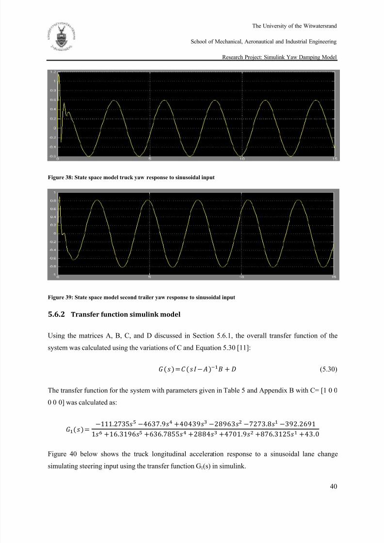
Figure 37 below shows the truck lateral acceleration response given by the state space model due to a
sinusoidal steering input function representing a lane change, while Figure 38 and Figure 39 show the
yaw response of the truck, and second trailers respectively.
Figure 37: State space model truck lateral acceleration response to sinusoidal input
8/13/2019 Simulink Yaw damping model
http://slidepdf.com/reader/full/simulink-yaw-damping-model 50/71
The University of the Witwatersrand
School of Mechanical, Aeronautical and Industrial Engineering
Research Project: Simulink Yaw Damping Model
40
Figure 38: State space model truck yaw response to sinusoidal input
Figure 39: State space model second trailer yaw response to sinusoidal input
5.6.2 Transfer function simulink model
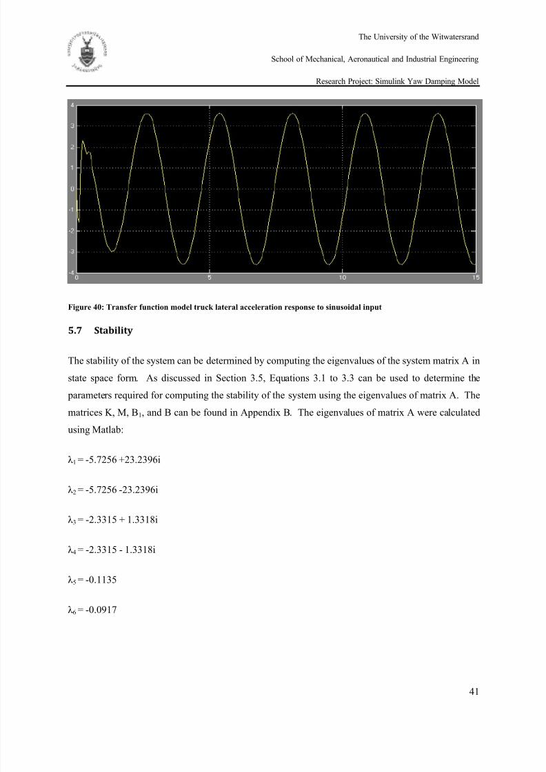
Using the matrices A, B, C, and D discussed in Section 5.6.1, the overall transfer function of the
system was calculated using the variations of C and Equation 5.30 [11]:
(5.30)
The transfer function for the system with parameters given in Table 5 and Appendix B with C= [1 0 0
0 0 0] was calculated as:
Figure 40 below shows the truck longitudinal acceleration response to a sinusoidal lane change
simulating steering input using the transfer function G1(s) in simulink.
8/13/2019 Simulink Yaw damping model
http://slidepdf.com/reader/full/simulink-yaw-damping-model 51/71
8/13/2019 Simulink Yaw damping model
http://slidepdf.com/reader/full/simulink-yaw-damping-model 52/71
The University of the Witwatersrand
School of Mechanical, Aeronautical and Industrial Engineering
Research Project: Simulink Yaw Damping Model
42
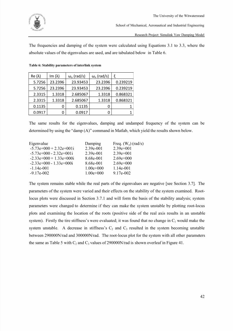
The frequencies and damping of the system were calculated using Equations 3.1 to 3.3, where the
absolute values of the eigenvalues are used, and are tabulated below in Table 6.
Table 6: Stability parameters of interlink system
Re (λ) Im (λ) ωo (rad/s) ωn (rad/s) ξ
5.7256 23.2396 23.93453 23.2396 0.239219
5.7256 23.2396 23.93453 23.2396 0.239219
2.3315 1.3318 2.685067 1.3318 0.868321
2.3315 1.3318 2.685067 1.3318 0.868321
0.1135 0 0.1135 0 1
0.0917 0 0.0917 0 1
The same results for the eigenvalues, damping and undamped frequency of the system can be
determined by using the “damp (A)” command in Matlab, which yield the results shown below.
Eigenvalue Damping Freq. (Wo) (rad/s)-5.73e+000 + 2.32e+001i 2.39e-001 2.39e+001-5.73e+000 - 2.32e+001i 2.39e-001 2.39e+001-2.33e+000 + 1.33e+000i 8.68e-001 2.69e+000-2.33e+000 - 1.33e+000i 8.68e-001 2.69e+000-1.14e-001 1.00e+000 1.14e-001
-9.17e-002 1.00e+000 9.17e-002
The system remains stable while the real parts of the eigenvalues are negative [see Section 3.7]. The
parameters of the system were varied and their effects on the stability of the system examined. Root-
locus plots were discussed in Section 3.7.1 and will form the basis of the stability analysis; system
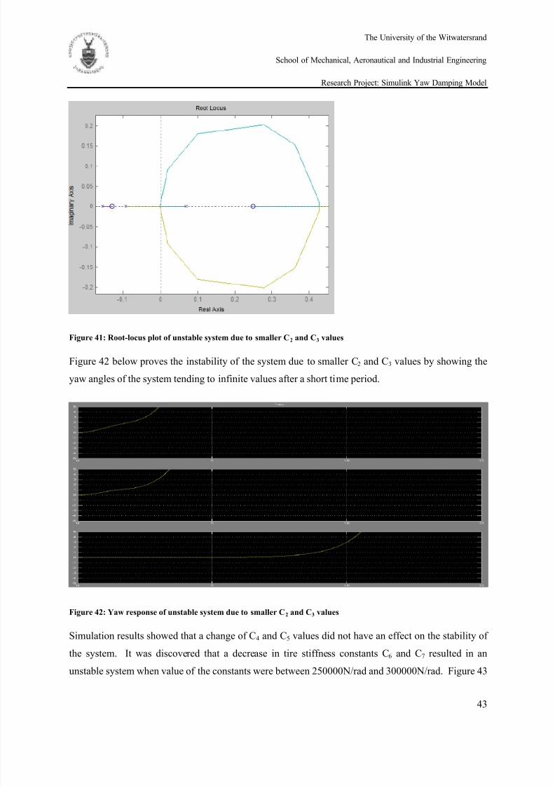
parameters were changed to determine if they can make the system unstable by plotting root-locus
plots and examining the location of the roots (positive side of the real axis results in an unstable
system). Firstly the tire stiffness’s were evaluated; it was found that no change in C1 would make the
system unstable. A decrease in stiffness’s C2 and C3 resulted in the system becoming unstable
between 290000N/rad and 300000N/rad. The root-locus plot for the system with all other parameters
the same as Table 5 with C2 and C3 values of 290000N/rad is shown overleaf in Figure 41.
8/13/2019 Simulink Yaw damping model
http://slidepdf.com/reader/full/simulink-yaw-damping-model 53/71
The University of the Witwatersrand
School of Mechanical, Aeronautical and Industrial Engineering
Research Project: Simulink Yaw Damping Model
43
Figure 41: Root-locus plot of unstable system due to smaller C2 and C3 values
Figure 42 below proves the instability of the system due to smaller C2 and C3 values by showing the
yaw angles of the system tending to infinite values after a short time period.
Figure 42: Yaw response of unstable system due to smaller C2 and C3 values
Simulation results showed that a change of C4 and C5 values did not have an effect on the stability of
the system. It was discovered that a decrease in tire stiffness constants C6 and C7 resulted in an
unstable system when value of the constants were between 250000N/rad and 300000N/rad. Figure 43
8/13/2019 Simulink Yaw damping model
http://slidepdf.com/reader/full/simulink-yaw-damping-model 54/71
The University of the Witwatersrand
School of Mechanical, Aeronautical and Industrial Engineering
Research Project: Simulink Yaw Damping Model
44
shows the root-locus plot of the unstable system with two roots marginally on the right hand side of
the plane.
Figure 43: Root-locus plot of unstable system due to smaller C6 and C7 values
The longitudinal velocity of the truck was increased to 34m/s which corresponds to just over120km/h. It was found that the system did not become unstable due to this increase; however, the
damping ratio has decreased, as well as the undamped frequency of the system as shown below:
Eigenvalue Damping Freq. (Wo) (rad/s)
-1.10e+001 + 1.38e+001i 6.23e-001 1.76e+001-1.10e+001 - 1.38e+001i 6.23e-001 1.76e+001
-1.37e+000 + 1.11e+000i 7.77e-001 1.77e+000-1.37e+000 - 1.11e+000i 7.77e-001 1.77e+000-9.35e-002 1.00e+000 9.35e-002-1.15e-001 1.00e+000 1.15e-001
An analysis into the effect of the masses of the components on the system showed that instability
occurs when m1 is decreased to almost 1000kg, which is an unrealistic mass of a truck unit. Neither
lowering the mass of the first trailer to 4156kg, which is the mass of the empty trailer, nor did
increasing it to 36000kg render the system unstable. Neither a decrease in m3 to 4415kg, which is the
empty load mass of the second trailer, nor an increase in m3 was found to affect the stability of the
system.
8/13/2019 Simulink Yaw damping model
http://slidepdf.com/reader/full/simulink-yaw-damping-model 55/71
The University of the Witwatersrand
School of Mechanical, Aeronautical and Industrial Engineering
Research Project: Simulink Yaw Damping Model
45
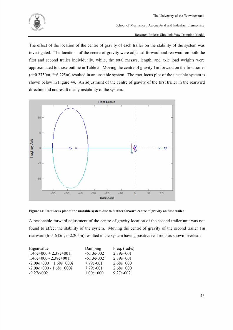
The effect of the location of the centre of gravity of each trailer on the stability of the system was
investigated. The locations of the centre of gravity were adjusted forward and rearward on both the
first and second trailer individually, while, the total masses, length, and axle load weights were
approximated to those outline in Table 5. Moving the centre of gravity 1m forward on the first trailer
(e=0.2750m, f=6.225m) resulted in an unstable system. The root-locus plot of the unstable system is
shown below in Figure 44. An adjustment of the centre of gravity of the first trailer in the rearward
direction did not result in any instability of the system.
Figure 44: Root locus plot of the unstable system due to further forward centre of gravity on first trailer
A reasonable forward adjustment of the centre of gravity location of the second trailer unit was not
found to affect the stability of the system. Moving the centre of gravity of the second trailer 1m
rearward (h=5.645m, i=2.205m) resulted in the system having positive real roots as shown overleaf:
Eigenvalue Damping Freq. (rad/s)1.46e+000 + 2.38e+001i -6.13e-002 2.39e+0011.46e+000 - 2.38e+001i -6.13e-002 2.39e+001-2.09e+000 + 1.68e+000i 7.79e-001 2.68e+000-2.09e+000 - 1.68e+000i 7.79e-001 2.68e+000-9.27e-002 1.00e+000 9.27e-002
8/13/2019 Simulink Yaw damping model
http://slidepdf.com/reader/full/simulink-yaw-damping-model 56/71
The University of the Witwatersrand
School of Mechanical, Aeronautical and Industrial Engineering
Research Project: Simulink Yaw Damping Model
46
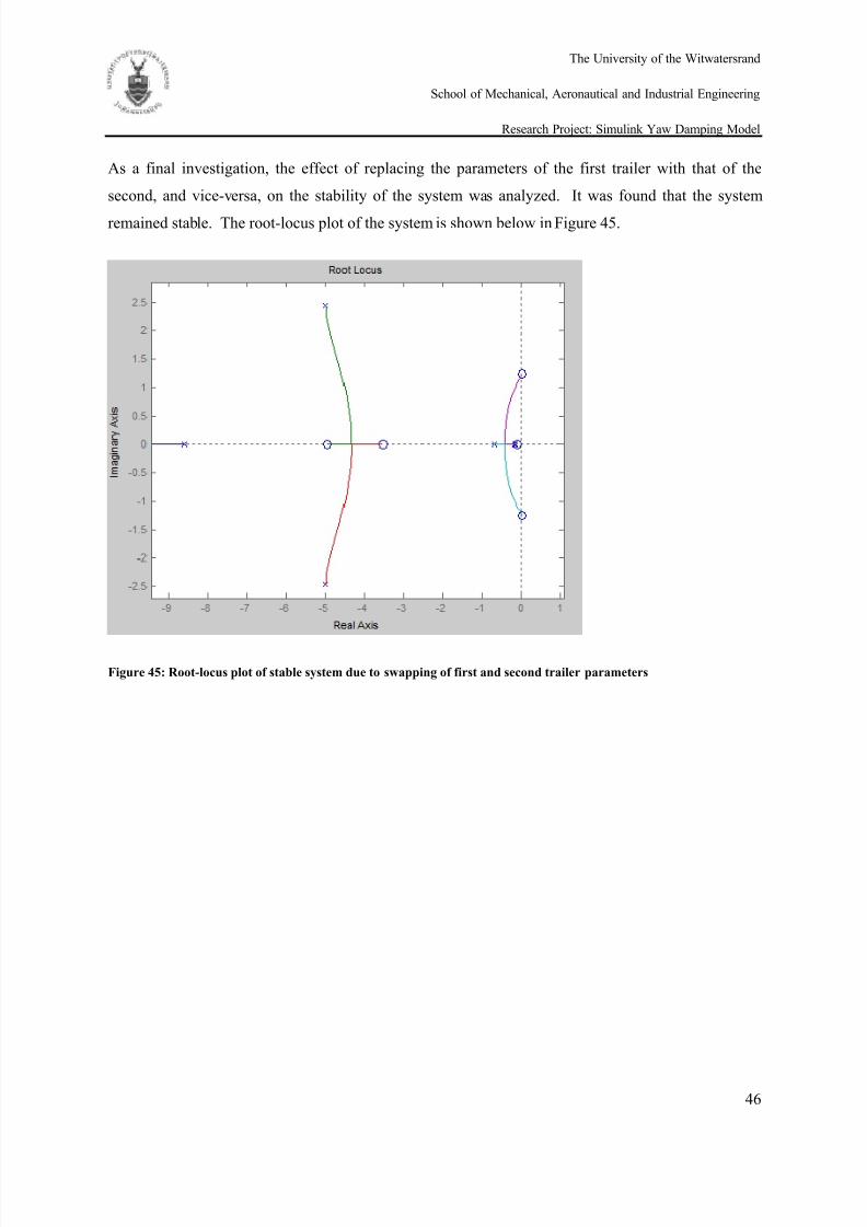
As a final investigation, the effect of replacing the parameters of the first trailer with that of the
second, and vice-versa, on the stability of the system was analyzed. It was found that the system
remained stable. The root-locus plot of the system is shown below in Figure 45.
Figure 45: Root-locus plot of stable system due to swapping of first and second trailer parameters
8/13/2019 Simulink Yaw damping model
http://slidepdf.com/reader/full/simulink-yaw-damping-model 57/71
The University of the Witwatersrand
School of Mechanical, Aeronautical and Industrial Engineering
Research Project: Simulink Yaw Damping Model
47
6 Discussion
The model derived in Section 5.2 of the interlink system shown in Figure 13 was based heavily on the
models derived in Section 4 of smaller, simpler systems. The model of a one truck and trailer system
derived in Section 4.2 produced identical simulation results to those published by [5],and this was
used to validate the designed simulink model of this system. The bicycle and Simulink model of the
interlink system was designed using the same methodology as that used to produce the valid model in
Section 4.2, and it was because of this, that the designed interlink Simulink model was determined to
be valid. No other validating texts of similar interlink model simulations could be found to verify the
model and no real life simulation were investigated, therefore, the entire model validation relies on the
model in Section 4.2 being valid.
The assumptions outlined in Section 5.1 were used to greatly simplify the real-life interlink system to
allow the simple bicycle model in Section 5.2 to be derived in order to be able to design a Simulink
model to, as accurately as possible, replicate the dynamic behaviour of the system due to a steering
input. The assumption about the symmetry of the vehicle mass and tire forces can be approximated to
be quite valid as a uniform load on a trailer would produce a symmetric mass distribution and, ideally,
the resultant reactant forces supplied by the tires would be the same. In a swerving manoeuvre, the
trailer would tend to roll from left to right in the restrictions of the suspension system which would
move the apparent centre of gravity of the load and decrease the accuracy of the model. The variation
of the longitudinal velocity of the vehicle was approximated to be negligible, which would hold
relatively true in situations where the magnitudes of the lateral velocities of the units are small relative
to the longitudinal velocity. The tires were assumed to roll without slipping in the longitudinal
direction which is true as the vehicle experienced no acceleration or breaking in this direction. The
lateral resultant forces from the tires was assumed to be linear which has some degree of accuracy
during small steering angles, however, some advanced texts have shown greater accuracy ofsimulation results by using a far more complicated non-linear tire model. The fixed connection
assumed at the kingpin between towing units is valid; however, a frictionless joint assumption could
prove to be far less accurate and should be investigated in further experimentation. The values of the
tire stiffness constants were calculated using Equation 5.23 published by [8] and [9], which makes use
of the loading supported by the tire. Without further means of calculating this value, the published
equation was deemed to be quite an accurate approximation, however, it is understood that different
tires may produce different stiffness’s which could change non-linearly over a range of loading
weights and, as discussed later, it was found that the stability of the system is to a large extent
8/13/2019 Simulink Yaw damping model
http://slidepdf.com/reader/full/simulink-yaw-damping-model 58/71
The University of the Witwatersrand
School of Mechanical, Aeronautical and Industrial Engineering
Research Project: Simulink Yaw Damping Model
48
dependent on the tire stiffness’s, therefore, a better analysis of these values should be performed in
future texts.
The bicycle model in Section 5.2 was used to derive equations of motion of the system detailed in
Section 5.3. The equations of motion were used to design the Simulink model to be used to
investigate the yaw rate, yaw angle, and lateral acceleration responses of the system to a steering
input. Furthermore, an investigation into the effects of varying the system parameters was performed
in Sections 5.5 and 5.7. The most accurate simulation results would be produced by a model in the
time-domain, which is shown in Figure 16. In addition to the time-domain model, far simpler
Simulink models were created using the state-space equations (Equations 5.28 and 5.29), and the
overall transfer functions of the system. Figure 23 shows the lateral acceleration response of the truck
to a sinusoidal steering input simulating a vehicle lane change produced by the time-domain model,
while Figures 37 and 40 show the same parameter response using the state space and transfer function
models respectively. It can be seen from the figures that the state-space and transfer function models
produce almost identical curves to the time-domain model after 0.5s of simulation, with magnitudes
being marginally different. A large instability and inaccuracy was noted in the initial response of the
simpler models as the initial conditions were inputted as zero; however, the steady state response was
only marginally inaccurate.
The first investigation performed was on the original interlink system with parameters as outlined in
Table 5. Figures 17, 18, and 19 show the yaw response of the system, over a 15s interval, to a
sinusoidal input with a frequency of 1.5Hz and amplitude of 0.1 which was deemed to simulate a lane
change by [5]. From the figures it can be concluded that the yaw angle amplitudes experienced by the
truck and the first trailer were similar with the trailer being marginally less. The yaw amplitudes
experienced by the second trailer were noticeably much smaller than the other two vehicles due to its
longer length and existence of yaw damping in the system. Interestingly, it is noted that the truck and
trailer were predicted to yaw symmetrically ‘left’ and ‘right’, while the second trailer has a tendency
to have a larger yaw magnitude in one direction than the other. The yaw rate responses shown in
Figures 20 to 22 are consistent with the yaw response curves with yaw acceleration decreasing
rearward along the system. With regards to the symmetry of the yaw experienced by the second
trailer, Figure 22 shows that the trailer experiences symmetrical yaw accelerations from 4 to -4x10⁻⁴
rad/s and it is therefore predicted that the phase difference between the yaw angles of the units results
in the second trailer not experiencing symmetrical yaw motion. As discussed in Section 3.1, the
lateral accelerations experienced by each unit are known to increase rearward from the towing unit,
8/13/2019 Simulink Yaw damping model
http://slidepdf.com/reader/full/simulink-yaw-damping-model 59/71
The University of the Witwatersrand
School of Mechanical, Aeronautical and Industrial Engineering
Research Project: Simulink Yaw Damping Model
49
known as the ‘rearward-amplification’ phenomena. The ‘rearward- amplification’ phenomena was
observed in the lateral acceleration responses produced by the interlink Simulink model, as shown in
Figure 24. The figure shows the lateral accelerations experienced by the truck (top curve) and the
first and second trailer units (second and third curves) in m/s2. From Figure 24, it was observed that
the truck experiences a maximum of approximately 5m/s acceleration in the lateral direction, while
the first trailer experiences marginally over 10m/s2 lateral acceleration and the third trailer
experiences a large maximum of 15m/s2 lateral acceleration from a simple lane change steering input
simulation. The rearward-amplification of the lateral acceleration responses shown in the figure is
consistent with known theory and results and can further be used to validate the accuracy of the
created Simulink model. It is known that the rolling over of heavy motor vehicles occurs initially
with the most rearward trailer rolling over first, this can be explained by the results shown in Figure
24 as the trailer with the largest mass is exposed to the largest lateral accelerations (more than twice
that of the towing unit), therefore, the momentum of the second trailer could easily cause the truck to
roll over in an evasive manoeuvre. As a final analysis, it is noted that the lateral acceleration response
curves are out of phase with one another and the second trailer experiences its largest acceleration
before the preceding units, even though the yaw response curves in Figures 17 to 19 only show a
marginal phase difference; again this is known to be due to the ‘rearward-amplification’ phenomena.
The steering input can vary from 0.15Hz in a normal lane change situation to approximately 4Hz in an
evasive manoeuvre [3]. A chirp signal in Simulink was used to vary a sinusoidal function linearly
over time from 0.15Hz to 4Hz to simulate the system response to an evasive manoeuvre. Figure 25
shows the yaw response of the system to this type of input over a 15s time period. From the figure, it
was noted that the yaw angle experienced by each unit again decreases rearward from the towing unit
and that the response decreases over time due to the damping of the system.
After the investigations of the dynamic responses of the initial system were completed, the effects of
varying different parameters of the system were explored. Firstly, the length of the second trailer was
changed to equal that of the first trailer, with masses and tire stiffness’s adjusted accordingly. Figure
26 shows the yaw rate response of the adjusted system to the same sinusoidal input as in Figures 20,
21, and 22 while Figure 27 shows the yaw response and 28 shows the lateral acceleration response.
Comparing Figures 26 and 27 to 20, 21, 22 and 17, 18, 19 it was noted that the truck and first trailer
experienced marginally lower yaw angles and yaw accelerations than in the original system, but the
second trailer experienced much larger accelerations and angles due to its decrease in length, mass
and tire stiffness’s. Furthermore, the lateral accelerations experienced by the truck and first trailer
8/13/2019 Simulink Yaw damping model
http://slidepdf.com/reader/full/simulink-yaw-damping-model 60/71
The University of the Witwatersrand
School of Mechanical, Aeronautical and Industrial Engineering
Research Project: Simulink Yaw Damping Model
50
were found not to have changed, while the lateral accelerations experienced by the second trailer were
found to have decreased, which would increase the stability of the system in a dynamic manoeuvre, as
shown by Figures 24 and 28. The consistency in the lateral accelerations experienced by the first two
units while the parameters of the third unit were varied show that a parameter change in rearward
units does not affect the lateral velocities experienced by leading units, there is therefore no feed
forward phenomenon and the lateral velocity systems can be said to be uncoupled.
The effects of increasing the length of first trailer to equal that of the second trailer and the second
trailer to equal that of the first (swapped) and adjusting masses and tire cornering stiffness’s
accordingly were also investigated. Figures 29, 30 and 31 show the dynamic responses of this system
to the sinusoidal lane change input. The most notable change in the system response can be found in
the lateral acceleration response curve in Figure 30, where it was noted that both the first and second
trailer experienced a large decrease in lateral acceleration (first trailer almost half) when compared
with the response shown in Figure 24. In terms of t a yaw angle analysis, it was noted that the
swapping of the trailers resulted in the second trailer experiencing almost twice the yaw angle than it
did in the original system with much larger yaw accelerations.
The tire cornering stiffness’s provide the reaction responses due to steering angles of the tires. As
discussed above, the stiffness’s were approximated using Equation 5.23. An investigation into the
effect that the tire cornering stiffness’s have on the dynamic response of the system was performed on
the original system with the parameters as outline in Table 5, but tire stiffness’s equal to 25% of the
originally estimated value. Figures 32 and 33 show the yaw rate and yaw response of the system to
the sinusoidal lane changing simulation. The yaw angles were found to decrease when compared to
the results in Figures 17, 18, and 19, while the yaw rates were found to increase due to the reduction
in tire cornering stiffness’s, resulting in the frequency of the yaw cycle to be increased. Furthermore,
instability can be seen during the initial part of the simulation until a steady state response was
attained. The tire cornering stiffness’s were predicted to have a large influence on the stability of the
system and it is noted that further experimentation should be performed to accurately calculate the
exact tire cornering stiffness’s of the model to validate the use of Equation 5.23.
Finally, an investigation into response of the system with a longitudinal velocity (u) of 34m/s
(approximately 120km/h) as opposed to 22.2m/s (approximately 80km/h) was performed. The yaw
rate response of the system with an increase in longitudinal velocity, subjected to the sinusoidal
steering input, is shown in Figure 34. Comparing the response to that shown in Figures 20, 21, and 22
shows a large increase in the yaw rate experienced by all units, while comparison of Figure 35 to
8/13/2019 Simulink Yaw damping model
http://slidepdf.com/reader/full/simulink-yaw-damping-model 61/71
The University of the Witwatersrand
School of Mechanical, Aeronautical and Industrial Engineering
Research Project: Simulink Yaw Damping Model
51
Figures 17, 18, and 19 show the corresponding increases in yaw angle experienced by the units with
the truck yaw angle increasing initially from approximately a maximum of 0.6rad to almost 1rad. The
first and second trailers have similar increases. Although it does not appear that the system has
become unstable due to the velocity increase, there is definitely a noticeable difference in the dynamic
behaviour of the system.
The system in comprised of many different parameters such as lengths and masses. The different
dynamic responses of the system that were observed during the experimentation when parameters
were changed led to the understanding that the changing of certain system parameters may render the
system to become unstable. A stability analysis was performed on the system with variable
configurations as outline in Section 5.7. Stability was summarised in Section 3.7 and root-locus plots
were used to determine the effect of the varying of different system parameters on the systems
stability. An observation of the root-locus plots while one parameter of the system was varied and
others were kept constant was performed to test whether the real part of the roots of the system
(marked with an ‘x’ on the figures) could become positive, or fall into the right hand side of the plane.
Firstly, the effect of the tire stiffness’s on the stability of the system was investigated because of the
prediction made previously that the system may become unstable due to a reduction in tire stiffness’s.
It was found that no amount of adjustment of stiffness C1 would make the system unstable. A
simultaneous decrease in stiffness’s C2 and C3, however, resulted in the root-locus plot shown in
Figure 41 which clearly shows a root in the right hand side of the plane and therefore an unstable
system. It was found that the system became unstable when C2 and C3 were decreased beyond
290000 and 300000N/rad. The time-domain Simulink model of the interlink system was used to test
the theory of the system becoming unstable with these parameters. It can be seen in Figure 42 that the
yaw response of the system due to the sinusoidal steering input rapidly tends to infinity after a short
period of time, proving that the system is thus unstable. Furthermore, the root-locus plot was
generated using the overall transfer function of the system discussed in Section 5.6.2 while the system
response plot was generated using the time-domain Simulink model, the correspondence between the
two completely separate methods again proves that very similar results can be attained from either
methodology. Simulation results showed that different values of stiffness’s C4 and C5 did not affect
the stability of the system, while Figure 43 shows that the system becomes unstable when C 6 and C7
were simultaneously reduced to between 250000 and 300000N/rad.
8/13/2019 Simulink Yaw damping model
http://slidepdf.com/reader/full/simulink-yaw-damping-model 62/71
The University of the Witwatersrand
School of Mechanical, Aeronautical and Industrial Engineering
Research Project: Simulink Yaw Damping Model
52
The increasing of the longitudinal velocity from 22.2m/s to 34m/s did not make the system unstable,
but the overall damping and damped natural frequency of the system were found to have decreased,
which would increase the susceptibility of the system instability if excited at a dangerous frequency.
An investigation into the effect that the mass of each unit has on the system was performed. The
moments of inertia and tire stiffness’s were adjusted accordingly. It was discovered that the mass of
the truck would have to be decreased beyond 1000kg to produce an unstable system, while the system
would remain stable under all other realistic loading situations where the masses could not be less
than that of an empty trailer or greater than that of any realistic value.
The positions of the centres of gravity on the trailers were altered and their effects on the stability of
the system recorded. The total mass of the load as well as the axle load weights and corresponding
tire stiffness’s were assumed to be unchanged from those outlined in Table 5 for simplicity. It was
discovered that moving the centre of gravity on the first trailer 1m forward resulted in an unstable
system as shown in the root-locus plot in Figure 44, while moving the centre of gravity 1m rearward
on the second trailer resulted in positive real roots and therefore an unstable system.
As a final investigation, the parameters of the trailers were swapped and the stability of the system
was analysed. Figure 45 shows the root-locus plot of the stable system produced which correspondsto the stability shown in Figures 29, 30, and 31 of the dynamic responses of the system with the
trailers swapped around.
8/13/2019 Simulink Yaw damping model
http://slidepdf.com/reader/full/simulink-yaw-damping-model 63/71
The University of the Witwatersrand
School of Mechanical, Aeronautical and Industrial Engineering
Research Project: Simulink Yaw Damping Model
53
7 Conclusion and Recommendations
The interlink truck system in Figure 13 was able to be accurately modeled in a simplified form of a
bicycle model as shown in Figures 14 and 15. The bicycle model was able to be created by making
assumptions with regards the behavior of the system and its surroundings. The model created was
used to be able to predict the dynamic response of the system with derived equations of motion with a
high degree of accuracy as discussed in Section 6.
The bicycle model of the interlink system was generated using the same methodology as that used to
generate the models of the one truck and truck and trailer systems as shown in Figures 3 and 6
respectively. The bicycle models shown in Figures 3 and 6 were used to accurately replicate the
dynamic responses of those systems using Simulink models and comparing the results to those
published by [3] and [5]. On the basis of the models generated in Sections 4.1 and 4.2 being accurate,
a Simulink model to predict the dynamic response of the interlink system was built using the bicycle
model in Figure 14 and validated methodology. The Simulink model created was able to predict the
yaw rate (rad/s), yaw angle (rad), and lateral acceleration (m/ss) responses of a system with the
parameters in Table 5 to different steering inputs simulating real driving conditions.
The yaw damping ratio of the system with parameters outlined in Table 5 operating at a longitudinal
velocity of 22.2m/s was able to be calculated. The yaw damping ratio between the truck and first
trailer was calculated to be 0.833, while the yaw damping ratio between the first and second trailer
was calculated to be 0.00102.
The time-domain Simulink model built in Section 5 was used to predict the dynamic behavior of the
system to steering inputs with different parameters to those outlined in Table 5. It was observed that
shortening the length and reducing the load mass of the second trailer increased the yaw response of
the second trailer to a sinusoidal input but decreased the lateral acceleration to which the unit was
exposed from 15m/ss to 12m/s
2. Replacing the first trailer with the properties of the second trailer and
vice versa, it was observed that the first trailer experienced marginally less yaw motion while the
second trailer yaw motion approximately doubled. The swapping of the trailers produced a reduction
in lateral accelerations to which the trailers were subjected to. A decrease in tire cornering stiffness’s
to 25% of the predicted value resulted in a large decrease in yaw experienced by the units, and the
system was able to be made unstable when the cornering stiffness’s C2, C3, C6, and C7 were decreased
beyond 300000N/rad as shown by the locus-plots in Figures 41 and 43 respectively. An increase in
8/13/2019 Simulink Yaw damping model
http://slidepdf.com/reader/full/simulink-yaw-damping-model 64/71
8/13/2019 Simulink Yaw damping model
http://slidepdf.com/reader/full/simulink-yaw-damping-model 65/71
8/13/2019 Simulink Yaw damping model
http://slidepdf.com/reader/full/simulink-yaw-damping-model 66/71
The University of the Witwatersrand
School of Mechanical, Aeronautical and Industrial Engineering
Research Project: Simulink Yaw Damping Model
56
9 References
1. Meuller, T.H., J.J., P.H., 1999. Heavy vehicle stability versus crash rates. 10-19.
2. Gerdes, J.C., 2002. Safety Performance and Robustness of Heavy Vehicle AVCS. California
PATH Program, w, 5-22.
3. Martini, R D, 2006. The Pennsylvania State University The Graduate School Department of
Mechanical and Nuclear Engineering- GPS/INS SENSING COORDINATION FOR VEHICLE
STATE IDENTIFICATION AND ROAD GRADE POSITIONING, 1, 22-30, 54-70.
4. Fancher, P.S., Segel, L., Winkler, C.B., Ervin, R.D. , 1984. Tracking and stability of multi-
unit truck combinations, UMTRI-84-25, 3-23, 50.
5. Maas, J. W. L. H. , 2006. Jackknife stability of a tractor semi-trailer combination. 9-11, 17-
25.
6. Dahlberg, E., Wideberg, J. P., 2004. INFLUENCE OF THE FIFTH-WHEEL LOCATION . 5-
11.
7. Ei-Gindy, M., N., X., 2001. Sensitivity of rearward amplification control of a truck/full trailer
to tire cornering stiffness variations. Journal of Automobile Engineering , Part D, 1-11.
8. Fancher, P.S., Generic Data for Representing Truck Tire Characteristics in Simulations of a
Braking and Braking-in-a-Turn Maneuvers. 1995, University of
Michigan Transport Research Institute (UMTRI).
9. Fancher, P.S., Bernard, J., Clover, C., Winkler, C., Representing Truck Tire Characteristics in
Simulations of Braking and Braking-in-a-Turn Maneuvers. Vehicle
System Dynamics, 1997. 27(Supp.): p. 207-220.
10. Henred Fruehauf, 2003. 6 and 12m Ultra lightweight Interlink Combination (All Steel).
11. Tewari, A, 2003. Modern Control Design with Matlab and Simulink . 1st ed. England: John
Wiley and Sons.
12. Claymore Engineering. 2004. Root Locus Analysis. [ONLINE] Available at:
http://claymore.engineer.gvsu.edu/~jackh/books/model/chapters/rootlocus.pdf.
[Accessed 10 September 12].
13. Cannon, R.H., Dynamics of Physical Systems, McGraw-Hill, 1967
14. Bucknell . 1818. Nyquist Plots. [ONLINE] Available at:
http://www.facstaff.bucknell.edu/mastascu/econtrolhtml/Freq/Freq6.html. [Accessed 05
September 12].
8/13/2019 Simulink Yaw damping model
http://slidepdf.com/reader/full/simulink-yaw-damping-model 67/71
The University of the Witwatersrand
School of Mechanical, Aeronautical and Industrial Engineering
Research Project: Simulink Yaw Damping Model
57
Appendix A
A.1 Derivation of equations of motion of one vehicle model
Σ forces in lateral direction:
Σ moments about z-axis:
Linear tire model approximation:
Slip angles (tire vector diagram):
ζ
y
x
Vf t
-αf
δf
Vf t
Vf
Vf x
ζ
8/13/2019 Simulink Yaw damping model
http://slidepdf.com/reader/full/simulink-yaw-damping-model 68/71
The University of the Witwatersrand
School of Mechanical, Aeronautical and Industrial Engineering
Research Project: Simulink Yaw Damping Model
58
Lateral velocity vector of front tire:
Longitudinal velocity vector:
Combining the above equations:
The rear tire has no steering angle, therefore:
Equations of motion with tire forces become:
Lateral acceleration in body-fixed coordinates:
Therefore, meaningful expressions of equations are given by:
A.2 Derivation of equations of motion of truck and trailer model
Performing a sum of forces and moments on the system produces three coupled equations of
motion:
( )
( )
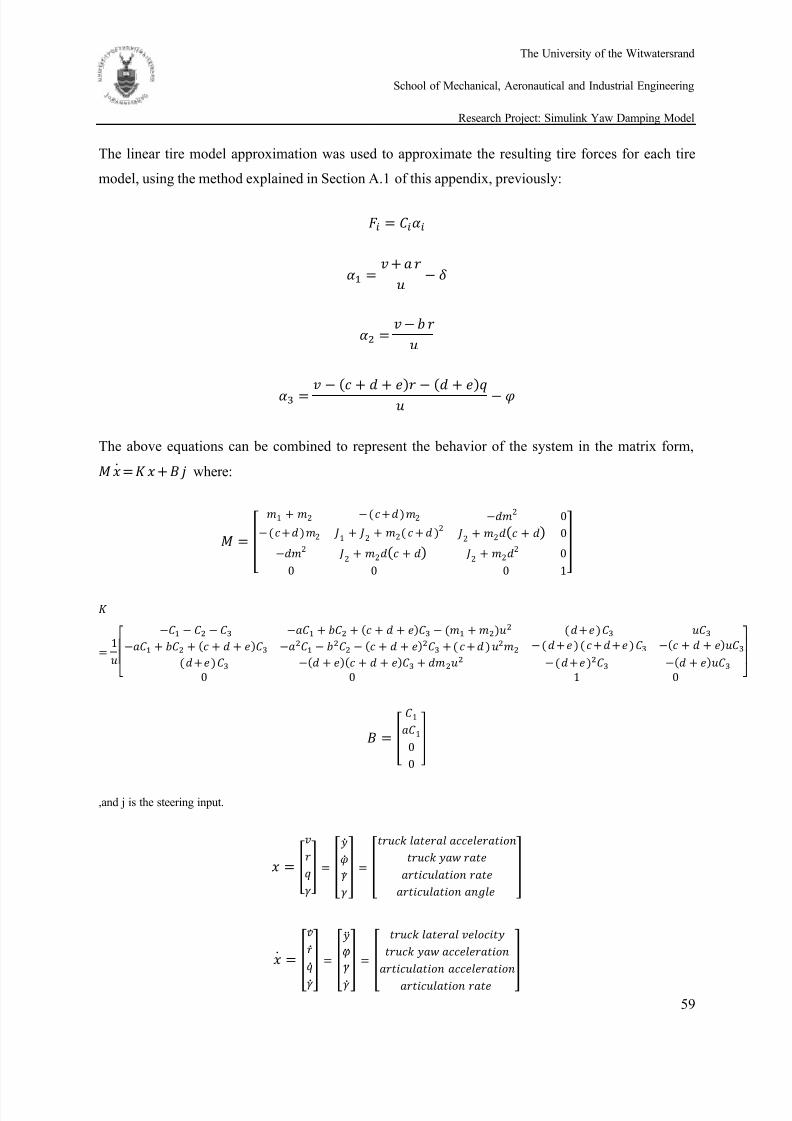
8/13/2019 Simulink Yaw damping model
http://slidepdf.com/reader/full/simulink-yaw-damping-model 69/71
The University of the Witwatersrand
School of Mechanical, Aeronautical and Industrial Engineering
Research Project: Simulink Yaw Damping Model
59
The linear tire model approximation was used to approximate the resulting tire forces for each tire
model, using the method explained in Section A.1 of this appendix, previously:
The above equations can be combined to represent the behavior of the system in the matrix form, where:
,and j is the steering input.
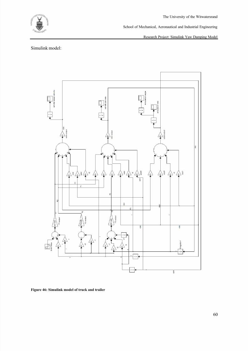
8/13/2019 Simulink Yaw damping model
http://slidepdf.com/reader/full/simulink-yaw-damping-model 70/71
The University of the Witwatersrand
School of Mechanical, Aeronautical and Industrial Engineering
Research Project: Simulink Yaw Damping Model
60
Simulink model:
Figure 46: Simulink model of truck and trailer
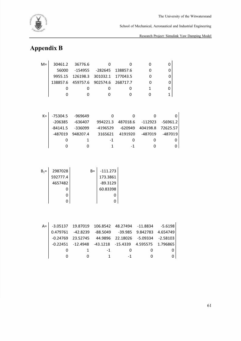
8/13/2019 Simulink Yaw damping model
http://slidepdf.com/reader/full/simulink-yaw-damping-model 71/71
The University of the Witwatersrand
School of Mechanical, Aeronautical and Industrial Engineering
Research Project: Simulink Yaw Damping Model
Appendix B
M= 30461.2 36776.6 0 0 0 0
56000 -154955 -282645 138857.6 0 0
9955.15 126198.3 301032.1 177043.5 0 0
138857.6 459757.6 902574.6 268717.7 0 0
0 0 0 0 1 0
0 0 0 0 0 1
K= -75304.5 -969649 0 0 0 0
-206385 -636407 994221.3 487018.6 -112923 -56961.2
-84141.5 -336099 -4196529 -620949 404198.8 72625.57
-487019 948207.4 3165621 4191920 -487019 -487019
0 1 -1 0 0 0
0 0 1 -1 0 0
B= -111.273
173.3861
-89.3129
60.83398
0
0
A= -3.05137 19.87019 106.8542 48.27494 -11.8834 -5.6198
0.479761 -42.8239 -88.5049 -39.985 9.842783 4.654749
-0.24769 23.52745 44.9896 22.18026 -5.09334 -2.58103-0.22451 -12.4948 -43.1218 -15.4339 4.595575 1.796865
0 1 -1 0 0 0
0 0 1 -1 0 0
B1= 2987028
592777.4
4657482
0
0
0