Diophantine equations in the primes

Invent. math.DOI 10.1007/s00222-014-0508-1

Diophantine equations in the primes

Brian Cook · Ákos Magyar

Received: 31 August 2013 / Accepted: 30 December 2013© Springer-Verlag Berlin Heidelberg 2014

Abstract Let p = (p1, . . . , pr ) be a system of r polynomials with integercoefficients of degree d in n variables x = (x1, . . . , xn). For a given r -tuple ofintegers, say s, a general local to global type statement is shown via classicalHardy-Littlewood type methods which provides sufficient conditions for thesolubility of p(x) = s under the condition that each of the xi ’s is prime.

Mathematics Subject Classfication (1991) 11D72 · 11P32

1 Background and main results

Let p = (p1, . . . , pr ) be a system of polynomials with integer coefficientsof degree d in the n variables x = (x1, . . . , xn). Our primary concern isfinding solutions with each coordinate prime, which we call prime solutionsto the system of equations p(x) = s, where s ∈ Z

r is a fixed element. In more

Ákos Magyar is supported by NSERC grant 22R44824 and ERC-AdG. 321104.

B. CookDepartment of Mathematics, University of Wisconsin–Madison, Madison,WI 53706-1325, USAe-mail: [email protected]

Á. Magyar (B)Department of Mathematics, The University of British Columbia, 1984 Mathematics Road,Vancouver, BC V6T 1Z2, Canadae-mail: [email protected]

123

B. Cook, A. Magyar

geometric terms, our task is to count prime points on the complex affine varietydefined by this equation, which we will denote by Vp,s.

If p is composed entirely of linear forms the known results may be split intoa classical regime and a modern one. With p being a system of r linear forms,define the rank of p to be the minimum number of nonzero coefficients in anon-trivial linear combination

λ1p1 + · · · + λrpr ,

and denote this quantity by B1(p). This quantity is of course positive if andonly if the forms are linearly independent. The classical results on the largescale distribution of prime points on Vp,s are conditional on the rank beingsufficiently large in terms of r (for example, 2r + 1 follows from what isshown here). In this realm are many well known results such as the ones dueto Vinogradov [18], van der Corput, and more recently Balog [1]. The modernresults are mostly summed up in the work of Green and Tao [7], where thelarge scale distribution of prime points on Vp,s is determined only on thecondition that B1(p) is at least three, a quantity independent of r . These resultscover all scenarios that do not reduce to a binary problem. However, the mostrecent result is due to Zhang. He has shown, by extending the already stunningresults of Goldston et al. [5], that one of the equations1 x1 − x2 = 2i, i =1, . . . , 35 × 106 does have infinitely many prime solutions [19].

The scenario for systems involving higher degree forms in certainly lessclean cut [4], and even the study of integral points on Vp,s is a non-trivialproblem. General results for the lag scale distribution of integral points areprovided by Birch [2] and Schmidt [17], which again require the system to belarge with respect to c notions of rank (with respect to the number and degreesof the forms involved). Working within the limitations of these results, oneshould expect to bable to understand the large scale distribution of prime pointsas well. For systems of forms which are additive, for instance the single forma1xd

1 +· · ·+anxdn , this is something that has been done and the primary result

here is due to Hua [11]. On the opposite end, if the system of forms is a bilinearsystem, or even contains a large bilinear piece, one can also provide similarresults, a particular instance of which is given by Liu [15] for a quadraticform. However, there have previously been no results for general systems ofnonlinear polynomials. Providing such a result is the aim of this work.

Before continuing it is worth discussing this problem from the point viewof some recent results in sieve theory. Let � ⊂ GLn(Z) be a finitely generatedsubgroup, O = �b be the orbit for some b ∈ Z

n , and g be an integral polyno-mial in n variables. Bourgain et al. in [3] initiated the study of a sieve method

1 The number of needed equations has been reduced by a poly-math project.

123


for finding points y ∈ O such that g(y) has few prime factors, provided ofcourse there are no obvious constraints. In particular they prove for suitablegroups that the almost prime points of the orbit form a Zariski dense subset,taking g to be the monomial form g(y) = y1 . . . yn . In case if a form f ispreserved by a sufficiently large group of transformations � ⊂ GLn(Z), thelevel sets Vf,s are partitioned into orbits of � and the methods of [3] show theexistence of almost prime solutions. The advantage is that one does not needthe largeness of the rank of the form, however, apart from quadratic forms,examples of such forms are quite rare (e.g. determinant forms), see [16] forthe study of integer solutions for such forms. Liu and Sarnak in [14] carryout this idea for indefinite quadratic forms in three variables, with � being thesubgroup of the special orthogonal group which preserves f. In particular, theyprove that one can find points on certain level sets of such quadratic formswhere each coordinate has at most 30 prime factors.

Returning to the problem at hand, for a fixed system of polynomials p letus define for each prime p the quantity

μp = limt→∞

(pt)r

M(

pt)

φn (pt ),

provided the limit exists, where M(

pt)

represents the number of solutions tothe equation p(x) = s in the multiplicative group of reduced residue classesmod pt , denoted by U n

pt , and φ is Euler’s totient function. A general heuristicargument suggests that we should have

Mp,s(N ) :=∑

x∈[N ]n

�(x)1Vp,s(x)

≈ μ∞(N , s)∏

p prime

μp(s) N n−D, (1.1)

where μ∞(N , s) is the singular integral that appears in the study of integralpoints on Vp,s, see [2], [17], � denotes the von Mangoldt function, D = dr ,and �(x) = �(x1)...�(xn).

What is actually shown here is a precise result of this form for systems ofpolynomials of common degree provided that the system has large rank inthe sense of Birch for the nonlinear forms and in the sense described abovefor linear forms. Let us be given a system of homogeneous polynomials f =(f1, . . . , fr ) with integer coefficients of degree exactly d. Define the singularvariety, over C

n , associated to the forms f to be the collection of x such that

123

B. Cook, A. Magyar

the Jacobian of f at x, given by the matrix of partial derivatives

Jac f(x) =[∂fk

∂x j(x)]r,n

k=1, j=1,

has rank strictly less than r . This collection is labeled as V ∗f . The Birch rank

Bd(f) is defined for d > 1 and is given by codim(

V ∗f

), provided that r �= 0. If

r = 0 then we simply assign the value ∞. This notion is extended to a generalpolynomial system p of degree d by defining the rank by Bd(p) = Bd(f),where f is the system of forms consisting of the highest degree homogeneousparts of the polynomials p. In particular, if the a system of forms has positiveBirch rank then the systems of forms f is a linearly independent system.

The main result that is shown here is the following.

Theorem 1 For given positive integers r and d, there exists a constant χ(r, d)such that the following holds:

Let p = p(d) be a given system of integral polynomials with r polynomialsof degree d in n variables, and set D = dr. If we have Bd(p) ≥ χ(r, d) thenfor the equation p(x) = s we have an asymptotic of the form

Mp,s(N ) =∏

p

μp(s) μ∞(N , s) N n−D + O(

N n−D(log N )−1)

Moreover, if p(x) = s has a nonsingular solution in Up, the p-adic integerunits, for all primes p, then

∏

p

μp(s) > 0.

Note that the singular integral μ∞(N , s) is the same as in the work of Birchand Schmidt (see [17], Sec.9 and [2], Sec.6). It is positive provided that thevariety Vf,N−d s has a nonsingular real point in the open cube (0, 1)n , and isbounded from below independently of N if there is a nonsingular real pointin the cube (ε, 1 − ε)n for some ε > 0. Indeed, the singular integral has therepresentation

∫

Vf,t∩[0,1]n

dσf(x), (1.2)

where t = N−d s, and dσf(x) is a positive measure on Vf,t\V ∗f which is

absolutely continuous with respect to the Euclidean surface area measure, seeBirch [2], Sec.6.

123


The quantitative aspects of the constants χ(r, d) are in general extremelypoor. The terms χ(r, 1) may be taken to be 2r + 1. The case for quadraticforms is still somewhat reasonable, for systems of quadratics one can show

χ(r, 2) ≤ 22Cr2

(to be compared to r(r+1) for the integral analogue). However,the constants χ(1, d) already exhibit tower type behavior in d (to be comparedto d2d for the integral analogue), and the situation further worsens from there.

A more detailed analysis of the singular series can be carried out it certaininstances to provide more concrete statements. This is not done here, howeverthere are some circumstances that have previously been considered. Borrowingthe results in this direction from Hua and Vinogradov gives the followingknown results (which are weaker than the best known for d > 1) for diagonalforms as a corollary. Note that for a diagonal form f of degree d in n variableswe have Bd(f) = n.

Corollary 1 Theorem 1 applies to diagonal integral forms f(x) = a1xd1 +

a2xd2 + · · · + anxd

n , a1a2 . . . an �= 0, when n ≥ 3 + (d − 1)2d . In particularif d = 1 and a1 = a2 = a3 = 1 one recovers the well known fact thatevery sufficiently large odd integer is a sum of three primes; if d = 2 anda1 = a2 = . . . = a7 = 1 then every sufficiently large integer congruent to 7modulo 24 is a sum of seven squares of primes.

Liu provides a general scenario to guarantee that the singular series is pos-itive for a single quadratic form. A quadratic form Q has the representation〈x, Ax〉 for some symmetric integral n × n matrix A. The Jacobian of theform is 2Ax, giving that the singular variety V ∗

Q is the null space of A, and soB(Q) = rank(A). A general condition for Q to be well behaved with respectto each prime modulus is that pn−2 does not divide det(A) for any prime p, asthen a simple consideration of eigenvalues shows that the matrix A has rankat least three when viewed over the finite field with p elements.

Corollary 2 Let Q(x) = 〈x, Ax〉 be an indefinite integral quadratic form in nvariables with rank(A) ≥ χ(2, 1) and pn−2

� det(A) for any prime p. ThenQ(x) = 0 has a solution in Up for all p if and only if Q(x) = 0 has a solutionwith xi prime for each i .

The value of χ(2, 1) can be worked out in directly with what is done in thispaper with minimal difficulty, and previously a value of 34 has been providedby the first author. Applying the results of Liu, as mentioned in the followingsection, is however more efficient and gives a value of 21. For the relatedproblem of finding integer solutions to a single quadratic equation Q(x) = 0in a set of positive upper density A ⊆ Z, Keil in [13] has recently obtained therank condition rank(Q) ≥ 17. The analogous statement for the integers is thefamous Hasse–Minkowski Theorem which requires no conditions on the rankor the determinant, and of course only looks at solubility in Zp and not Up.

123

B. Cook, A. Magyar

2 Overview

The primary technique used in the proof of Theorem 1 is the circle method,and the argument is an adaptation of the following mean value approach. If asingle integral form F of degree d in n variables takes the shape

F(x) = xd1 + F1(y)+ F2(z), (2.1)

where x = (x1, y, z), then we have the representation

MF,0 =1∫

0

⎛

⎝∑

x1∈[N ]�(x1)e

(αxd

1

)⎞

⎠

⎛

⎝∑

y∈[N ]m

�(y)e(αF1(y))

⎞

⎠

×⎛

⎝∑

z∈[N ]n−1−m

�(z)e(αF2(z))

⎞

⎠ dα :=1∫

0

S0(α)S1(α)S2(α)dα.

An application of the Cauchy–Schwarz inequality then gives

M2F,0 ≤ ||S0||2∞||S1||22||S2||22 ≤ ||S0||2∞(log N )2n−2Y (N )Z(N ),

where Y (N ) is the number of solutions to the equation F1(y) = F1(y′) withy, y′ ∈ [N ]m and Z(N ) is the number of solutions to the equation F2(z) =F2(z′) with z, z′ ∈ [N ]n−1−m . If F1 and F2 are assumed to have large rank,then Y (N )Z(N ) = O

(N 2m−d

)O(N 2(n−1−m)−d

) = O(N 2n−2−2d

). More

generally, for any measurable subset u ⊂ [0, 1] we have

∫

u

S0(α)S1(α)S2(α)dα = O(||S0||∞(u)(log N )n−1 N n−1−d

), (2.2)

where ||S0||∞(u) denotes the supremum of |S0(α)| for α ∈ u.Then a partition into so-called major arcs M(C) and minor arcs m(C),

depending on a parameter C (see Sect. 5 for the precise definitions), becomesuseful due to the following fundamental estimate of Hua and Vinogradov

Lemma 1 [11] Given c > 0, there exists a constant C > 0 such that||S0||∞(m(C)) ≤ N (log N )−c.

This, together with Eq. 2.2, in turn gives the bound

∫

m(C)

S0(α)S1(α)S2(α)dα = O((log N )−1 N n−d

), (2.3)

123


and one is left with the task of approximating the integral over the major arcs

∫

M(C)

∑

x∈[N ]n

e(αF(x))dα.

Without going into the details here, let us remark that the major arcs consist ofvery small intervals (or boxes) centered at rational points with small denomina-tors, and the integral essentially depends only on the distribution of the valuesof the polynomials F(x) in small residue classes. Then the approximation canbe done via standard methods in this area, similarly as in the diagonal case[11].

Now let us look at the case of a general form F of degree 2. If we introducea splitting of the variables x = (x1, y, z), we induce a decomposition of theshape

F(x) = ax21 + g(1)(y, z)x1 + F1(y)+ F2(z)+ g(2)(y, z)

for a form g(2) which is bilinear in y and z, and a linear form g(1). There aretwo possible approaches to adapting the above argument to this case.

The first involves a dichotomized argument based on the rank of g(2). If wehave that g(2) has large rank, one can obtain good bounds on the exponentialsum

∑

y∈[N ]m

∑

z∈[N ]n−1−m

�(y)�(z)e(α(F1(y)+ F2(z)+ g(2)(y, z)+ x1g(1)(y, z))))

by simply removing the contribution of the von Mangoldt function with twoapplications of the Cauchy–Schwarz inequality. During this process the x1variable differences out, and the x1 summation may be treated trivially. In thiscase the methods of Birch [2] are applicable (and the rank bounds are compa-rable, see [15]). If g(2) has small rank, then it must be the case that F1 and F2each have large rank for appropriately chosen splitting of the variables. Writeg(2)(y, z) = 〈y, Bz〉 for an appropriately sized matrix B whose rank is small,and split g(1)(y, z) = l1(y)+ l2(z). The above argument can then be run on theintersection of the level sets of l1(y), l2(z), and Bz, as the form F(x) takes thediagonal shape given in (2.1), and both F1 and F2 have large rank on this smallco-dimensional affine linear space. On such an intersection we get an extrapower gain, which is equal to its codimension which then compensates for theloss of originally applying the Cauchy–Schwarz inequality on each level set.Thus summing the estimates over all such level sets gives an appropriate bound.

The second approach, to be fair, is simply a streamlined version of the firstwhich removes the need for a dichotomized approach, and this is the one we

123

B. Cook, A. Magyar

shall follow. The main requirement here is an appropriate decomposition of Fin the form

F(x) = ax21 + g(1)(y, z)x1 + F1(y)+ F2(z)+ g(2)(y, z)

such that the rank of F1 + g(2) is sufficiently large, the number of variables ofcomposing y, say m, is controlled, and the rank of F2 is large with respect to m.As before, we wish to fix l1(y), l2(z), and Bz. The difference is that we have noassumption on the rank of B. However, by controlling the value of m, we havea way to control the number of linear equations in z. Running the argumentas before and summing over the level sets reduces the minor arcs estimates toproviding an appropriate bound for the number of solutions to the system

F1(y)+ g(2)(y, z) = F1(y′)+ g(2)(y′, z)

l1(y) = l1(y′)F2(z) = F2(z′) (2.4)

l2(z) = l2(z′)Bz = Bz′

with y, y′ ∈ [N ]m and z, z′ ∈ [N ]n−1−m . This is achieved by the rank assump-tions of F1 + g(2) and F2 in the original decomposition.

The strategy for forms of higher degree starts by a similar decompositionof the form

F(x) = axd1 + g(1)(y, z)xd−1

1 + · · · + g(d−1)(y, z)x1

+F1(y)+ F2(z)+ g(d)(y, z),

where the g(i) are forms of degree i , and F1(y), F2(z), g(d) are forms of degreed. Again we require that the rank of F1 + g(d) is large with respect to g(i) foreach i < d, the number of variables m composing y is small, and the rank of F2is large with respect to m. That such a decomposition is possible is the subjectof Sect. 4. Then we view each form g(i), 1 ≤ i ≤ d, as a sum of forms in y withcoefficients that are forms in z, and the number of these coefficients is boundedin terms of m and d. On each of the level sets of this new system of forms in zwe have a system of forms in y, the number of which is bounded in terms ofd. Now passing to the further level of sets of these forms y provides a placeto carry out the simple Cauchy–Schwarz argument at the beginning of thissection. Summing back over the level sets then provides a system analogousto the one above.

The only problem with this so far is that the system we end up with containsat least a portion of each form g(i)(y, z) for i = 1, . . . , d, and we have no

123


control on the rank of these forms at all and therefore have no way of dealingwith the terminal system. The solution to this problem is found in the workof Schmidt [17]. His results provide a way of partitioning the level sets of aform by the level sets of a system of forms that does have high rank in eachdegree. Section 3 is dedicated to this. Working with this more regular systemas opposed to the g(i)’s does provide a manageable terminal system, and allowsfor a bound on the minor arc integral.

Extending this method to systems of forms is relatively straightforward atthis point, and is of course carried out below. The major technical difficultyhere is the need to isolate larger number of suitable variables x1, . . . , xK toget the logarithmic gain on the minor arcs, as opposed to a randomly chosensingle variable x1.

2.1 Outline and notation

The outline for the rest of the paper is as follows. Sections 3 and 4 are asdescribed above. The completion of the bound for the integral over the minorarcs is going to be carried out in Sect. 5. The major arcs are dealt with in Sect. 6,where the asymptotic formula is shown. Section 7 is dedicated to the proof ofTheorem 1. The final section concludes the work with a few further remarks.

Remarks on notation The symbols Z, Q, R, and C denote the integers, therational numbers, the real numbers, and the complex numbers, respectively.The r -dimensional flat torus R

r/Zr is denoted by Tr . The p-adic integers

are denoted by Zp, and the units of Zp are denoted by Up. The symbol Z Nrepresents shorthand for the groups Z/NZ. Also, the shorthand for the multi-plicative group reduced residue classes Z∗

N is UN .For a given measurable set X ⊆ T

r we shall use the notation || f ||p(X)to denote the L p norm of the function 1X f with the normalized Lebesguemeasure on the r -dimensional flat torus. If X is omitted it is assumed thatX = T

r . Here, and in general, 1X denotes a characteristic function for Xin a specified ambient space, and, on occasion, the set X is replaced by aconditional statement which defines it.

The Landau o and O notation is used throughout the work. The notationf � g is sometimes used to replace f = O(g). The implied constants areindependent of N and s, but may depend on all other parameters such as d, r ,n, and p.

3 A regularity lemma

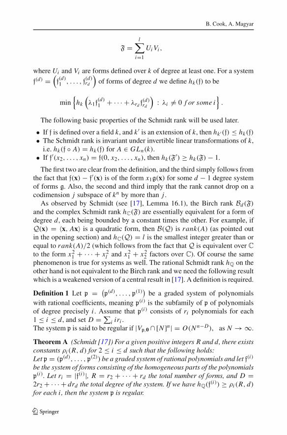
In [17], Schmidt provides an alternative definition of rank for a form. For asingle form F of degree at least 2 defined over a field k, define the Schmidt rankhk(F) to be the minimum value of l such that there exists a decomposition

123

B. Cook, A. Magyar

F =l∑

i=1

Ui Vi ,

where Ui and Vi are forms defined over k of degree at least one. For a system

f(d) =(f(d)1 , . . . , f

(d)rd

)of forms of degree d we define hk(f) to be

min{

hk

(λ1f

(d)1 + · · · + λrd f

(d)rd

): λi �= 0 f or some i

}.

The following basic properties of the Schmidt rank will be used later.

• If f is defined over a field k, and k′ is an extension of k, then hk′(f) ≤ hk(f)• The Schmidt rank is invariant under invertible linear transformations of k,

i.e. hk(f ◦ A) = hk(f) for A ∈ GLn(k).• If f′(x2, . . . , xn) = f(0, x2, . . . , xn), then hk(F

′) ≥ hk(F)− 1.

The first two are clear from the definition, and the third simply follows fromthe fact that f(x) − f′(x) is of the form x1g(x) for some d − 1 degree systemof forms g. Also, the second and third imply that the rank cannot drop on acodimension j subspace of kn by more than j .

As observed by Schmidt (see [17], Lemma 16.1), the Birch rank Bd(F)and the complex Schmidt rank hC(F) are essentially equivalent for a form ofdegree d, each being bounded by a constant times the other. For example, ifQ(x) = 〈x, Ax〉 is a quadratic form, then B(Q) is rank(A) (as pointed outin the opening section) and hC(Q) = l is the smallest integer greater than orequal to rank(A)/2 (which follows from the fact that Q is equivalent over C

to the form x21 + · · · + x2

l and x21 + x2

2 factors over C). Of course the samephenomenon is true for systems as well. The rational Schmidt rank hQ on theother hand is not equivalent to the Birch rank and we need the following resultwhich is a weakened version of a central result in [17]. A definition is required.

Definition 1 Let p = (p(d), . . . , p(1)

)be a graded system of polynomials

with rational coefficients, meaning p(i) is the subfamily of p of polynomialsof degree precisely i . Assume that p(i) consists of ri polynomials for each1 ≤ i ≤ d, and set D =∑i iri .The system p is said to be regular if |Vp,0 ∩ [N ]n| = O(N n−D), as N → ∞.

Theorem A (Schmidt [17]) For a given positive integers R and d, there existsconstants ρi (R, d) for 2 ≤ i ≤ d such that the following holds:Let p = (p(d), . . . , p(2)) be a graded system of rational polynomials and let f(i)

be the system of forms consisting of the homogeneous parts of the polynomialsp(i). Let ri = |f(i)|, R = r2 + · · · + rd the total number of forms, and D =2r2 + · · · + drd the total degree of the system. If we have hQ(f

(i)) ≥ ρi (R, d)for each i , then the system p is regular.

123


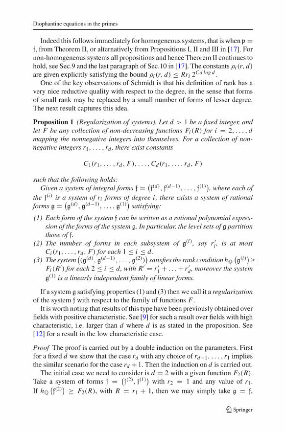
Indeed this follows immediately for homogeneous systems, that is when p =f, from Theorem II, or alternatively from Propositions I, II and III in [17]. Fornon-homogeneous systems all propositions and hence Theorem II continues tohold, see Sec.9 and the last paragraph of Sec.10 in [17]. The constants ρi (r, d)are given explicitly satisfying the bound ρi (r, d) ≤ Rri 2Cd log d .

One of the key observations of Schmidt is that his definition of rank has avery nice reductive quality with respect to the degree, in the sense that formsof small rank may be replaced by a small number of forms of lesser degree.The next result captures this idea.

Proposition 1 (Regularization of systems). Let d > 1 be a fixed integer, andlet F be any collection of non-decreasing functions Fi (R) for i = 2, . . . , dmapping the nonnegative integers into themselves. For a collection of non-negative integers r1, . . . , rd , there exist constants

C1(r1, . . . , rd , F), . . . ,Cd(r1, . . . , rd , F)

such that the following holds:Given a system of integral forms f = (f(d), f(d−1), . . . , f(1)

), where each of

the f(i) is a system of ri forms of degree i , there exists a system of rationalforms g = (g(d), g(d−1), . . . , g(1)

)satisfying:

(1) Each form of the system f can be written as a rational polynomial expres-sion of the forms of the system g. In particular, the level sets of g partitionthose of f.

(2) The number of forms in each subsystem of g(i), say r ′i , is at most

Ci (r1, . . . , rd , F) for each 1 ≤ i ≤ d.(3) The system

((g(d), g(d−1), . . . , g(2))

)satisfies the rank condition hQ

(g(i))≥

Fi (R′) for each 2 ≤ i ≤ d, with R′ = r ′1 + . . .+ r ′

d , moreover the systemg(1) is a linearly independent family of linear forms.

If a system g satisfying properties (1) and (3) then we call it a regularizationof the system f with respect to the family of functions F .

It is worth noting that results of this type have been previously obtained overfields with positive characteristic. See [9] for such a result over fields with highcharacteristic, i.e. larger than d where d is as stated in the proposition. See[12] for a result in the low characteristic case.

Proof The proof is carried out by a double induction on the parameters. Firstfor a fixed d we show that the case rd with any choice of rd−1, . . . , r1 impliesthe similar scenario for the case rd + 1. Then the induction on d is carried out.

The initial case we need to consider is d = 2 with a given function F2(R).Take a system of forms f = (

f(2), f(1))

with r2 = 1 and any value of r1.If hQ

(f(2)) ≥ F2(R), with R = r1 + 1, then we may simply take g = f,

123

B. Cook, A. Magyar

otherwise f(2) = ∑li=1 Ui Vi for some rational linear forms Ui and Vi where

l < F2(R). We may then adjoin the linear forms U1, . . . , Vl to the systemf(1) to obtain the system g(1), and let g be a maximal linearly independentsubsystem of g(1). Properties (1) and (2) are easily verified for this system,and property (3) is immediate.

Now for a fixed value of d assume that the result holds for all systemswith maximal degree d for any given collection of functions F when rd = jand rd−1, . . . , r1 are arbitrary. Consider now a fixed collection of functionsF and a system f = (

f(d), . . . , f(1))

with rd = j + 1. Let f′ be the system(f(d−1), . . . , f(1)

). By the induction hypothesis, there is a system g′ of rational

forms which is a regularization of f′ with respect to F ′i (R) := Fi (R + ( j +1))

for i = 2, . . . , (d − 1).Now let g′ = (

f(d), g′). If g′ fails to be the regularization of f with respectto the family of functions F , then hQ

(f(d))< Fd

(Rg′ + ( j + 1)

), where

Rg′ is the number of forms of the system g′. As before, in this case theremust exist homogeneous rational polynomials Ui and Vi , i = 1, . . . , l <Fd(Rg′ + ( j + 1)), such that

λ1f(d)1 + . . . λ j+1f

(d)j+1 =

∑

i≤l

Ui Vi ,

where without loss of generality we may assume that λ j+1 �= 0. Now let g′′ beg′ adjoined with the those forms Ui and Vi which are not linear combinationsof forms already in g′, and set

g′′ =((

f(d)1 , . . . , f

(d)j

), g′′) .

By the induction hypothesis there is a system g which is the regularization of g′′with respect to initial collection of functions F . It is clear from the constructionof the system g that all forms of the initial system are polynomial expressionsof the ones in g, and the number of forms in each subsystem g(i) is expressiblein terms of r1, . . . , rd , and d. Thus the system g is the regularization of fsatisfying conditions (1), (2) and (3). The induction argument to go from d tod + 1 is simply the above argument carried out with j = 0. ��

We will need a stronger version of the above proposition relative to a parti-tion of the variables x = (y, z). To state it let us introduce a modified versionof the Schmidt rank. For a single form F(y, z) of degree at least 2 defined overa field k, we define its Schmidt rank with respect to the variables z, hk(F; z)to be the minimum value of l such that there exists a decomposition

123


F(y, z) =l∑

i=1

Ui (y, z)Vi (y, z)+ W (z),

where Ui and Vi are forms defined over k of degree at least one. For a system

f(d) =(f(d)1 , . . . , f

(d)rd

)of forms of degree d we define hk(f; z) to be

min{

hk

(λ1f

(d)1 + · · · + λrd f

(d)rd

; z)

: λi �= 0 f or some i},

and set hk(f; z) = ∞ if f = ∅. Note that hk(f; z) ≤ hk(f) and hk(f; z) = 0 ifand only if a non-trivial linear combination of the forms in f depends only onthe variables z.

Proposition 1’ (Regularization of systems, parametric version). Let d > 1be a fixed integer, and let F be any collection of non-decreasing functionsFi (R) for i = 2, . . . , d mapping the nonnegative integers into themselves. Fora collection of non-negative integers r1, . . . , rd , there exist constants

C1(r1, . . . , rd , F), . . . ,Cd(r1, . . . , rd , F)

such that the following holds:Given a system of integral forms f = (f(d), f(d−1), . . . , f(1)

)where each of the

f(i) is a system of ri forms of degree i and a partition of the variables x = (y, z),there exists a system of rational forms g = (g(d), g(d−1), . . . , g(1)

)satisfying:

(1) Each form of the system f can be written as a rational polynomial expres-sion of the forms of the system g. In particular, the level sets of g partitionthose of f.

(2) The number of forms in each subsystem of g(i), say r ′i , is at most

Ci (r1, . . . , rd , F) for each 1 ≤ i ≤ d.(3) The system

(g(d), g(d−1), . . . , g(2)

)satisfies the rank condition hQ(g

(i)) ≥Fi (R′) for each 2 ≤ i ≤ d, with R′ = r ′

1 + . . .+ r ′d , moreover the system

g(1) is a linearly independent family of linear forms.(4) The system

(g(d), g(d−1), . . . , g(2)

)satisfies the modified rank condition

hQ

(g(i); z

) ≥ Fi (R′) for each 2 ≤ i ≤ d, where the subsystem g(i) isobtained from the system g(i) by removing the forms depending only onthe z variables.

We call a system g satisfying the conclusions of Proposition 1’ to be a strongregularization of the system f with respect to the variables z.

Proof The argument is a slight modification of the proof of Proposition 1. To agiven system f = (f(d), f(d−1), . . . , f(1)

)we assign its index which is the triple

123

B. Cook, A. Magyar

(d, rd , r ′d), where rd = ∣

∣f(d)∣∣ resp. rd = ∣

∣f(d)∣∣ are the number of degree d

forms resp. the number of degree d forms depending on at least one of the yvariables. We will proceed via induction on the lexicographic ordering of theindexes. To be precise we deem (d, rd , rd) ≺ (e, re, re) if d < e, d = e butrd < re, or d = e, rd = re but rd < re.

If d = 1 all one needs to do is to choose maximal linearly independentsubsystem of f = f(1). So assume d ≥ 2 (and rd ≥ 1), I = (d, rd , rd) is afixed index and the result holds for any system with index I ′ ≺ I . Again, letf′ = (f(d−1), . . . , f(1)

)and let g′ be a strong regularization of f′ with respect to

the functions F ′i (R) = Fi (R + rd) (i = 2, . . . , d − 1) and the variables z. Let

g′ = (f(d), g′). If g′ fails to be a strong regularization of f with respect to the

family of functions F and the variables z, then there are two possible cases.Either hQ

(f(d))< Fd(Rg′ + rd), where Rg′ is the number of forms of the

system g′. As before, in this case one can replace the system g′ with with asystem g′′ of index I ′′ ≺ I . Then by the induction hypotheses there is a systemg which is a strong regularization of g′′ with respect to initial collection offunctions F and the variables z. The system g will satisfy the claims of theproposition.

Otherwise rd ≥ 1 and we have hQ

(f(d); z

)< Fd(Rg′ + rd), hence there

must exist homogeneous rational polynomials Ui and Vi , i = 1, . . . , l <Fd(Rg′ + rd), and a form Q(z) of degree d such that

λ1f(d)1 +. . . λrd f

(d)rd

=∑

i≤l

Ui (y, z)Vi (y, z)+Q(z),(f(d)=

(f(d)1 , . . . , f

(d)rd

))

where without loss of generality we may assume that λrd �= 0. Now let g′′ beg′ adjoined with the those forms Ui and Vi which are not linear combinationsof forms already in g′, and set

g′′ =((

f(d)\f(d)rd, Q), g′′) .

Note that we have replaced the form f(d)rd(y, z) with the form Q(z) hence the

index of g′′ is the triple I ′′ = (d, rd , rd − 1) ≺ I . Again, there is a systemg which is a strong regularization of g′′ with respect to initial collection offunctions F and the variables z. As explained before the system g satisfies theclaims of the proposition. Note that the procedure depends on the partition x =(y, z), however since there only finitely many ways to partition the variablesx, the constants Ci (r1, . . . , rd , F) can be taken independent of the partition. ��

Applying Proposition 1’ with the functions being given by the values of theSchmidt constants ρi (R, d) then provides the following.

123


Corollary 3 Let f = (f(d), . . . , f(2)

)be given system of rational forms with

ri forms of degree i composing each subsystem f(i) and let x = (y, z) be apartition of the independent variables. There exists a regular system of formsg satisfying the conclusions of Proposition 1’.

Proof For fixed d, let g be a strong regularization of the system f with respectto the functions Fi (R) := ρi (R, d) + R and the variables z. We show that|Vg,0 ∩ [N ]n| = O(N n−R).

Let H := Vg(1),0 be the nullset of the system g(1), and let A ∈ GLn(Q)

be a linear transformation such that M := A(H) is coordinate subspace ofcodimension r1. It is easy to see that A([N ]n) ⊆ K −1

1 · [−K2 N , K2 N ]n forsome constants K1 and K2, where by λ · x we mean a dilation of the point xby a factor λ. Let g′ = g ◦ A−1, then Vg′,0 = A(Vg,0), thus by homogeneitywe have that

|Vg,0 ∩ [N ]n| ≤ |Vg′,0 ∩ [−K N , K N ]n|, (3.1)

with K = K1K2. We have that hQ

(g′(i)) = hQ

(g(i)) ≥ Fi (R), and hence

hQ

(g′(i)|M

) ≥ ρi (R, d), for i = 2, . . . , d, where R denotes the total numberforms of g′. The quantity on the right side of (3.1) is the number of integralpoints x in M ∩ [−K N , K N ]n = [−K N , K N ]n−r1 such that g′(i)(x) = 0for i = 2, . . . , d. Since the system

(g′(d), . . . , g′(2)) satisfies the conditions of

Theorem A, we have that |Vg′,0 ∩ [−K N , K N ]n| = O(N n−R

). This proves

the corollary. ��The somewhat technical last conclusion in Proposition 1’ is utilized in the

following lemma which will play an important role in our minor arcs estimates.

Lemma 2 Let g(k)(y, z) =(g(k)1 (y, z), . . . , g(k)s (y, z)

)be system of homoge-

neous forms of degree k. Then for the system g(k)(y, y′, z) = (g(k)(y, z), g(k)

(y′, z))

we have that

hQ

(g(k); z

)= hQ

(g(k); z

).

Here y, y′ and z represent distinct sets of variables.

Proof Since g(k) is a subsystem of g(k) it is clear that hQ

(g(k); z

) ≤hQ

(g(k); z

). Now let λ, μ be s-tuples of rational numbers not all 0. Using

the short hand notation λ · g(k) =∑i λig(k)i assume that we have a decompo-

sition

λ · g(k)(y, z)+ μ · g(k)(y′, z) =h∑

i=1

Ui (y, y′, z)Vi (y, y′, z)+ Q(z), (3.2)

123

B. Cook, A. Magyar

where all forms Ui , Vi have positive degree. We argue that h ≥ hQ(g(k)).

Assuming without loss of generality that λ �= 0 and substituting y′ = 0 into(3.2) we have

λ · g(k)(y, z) =h∑

i=1

Ui (y, 0, z)Vi (y, 0, z)+ Q′(z),

with Q′(z) = Q(z) − μ · g(k)(0, z). For each 1 ≤ i ≤ h the termUi (y, 0, z)Vi (y, 0, z) vanishes identically or both forms Ui (y, 0, z) andVi (y, 0, z) have positive degrees, thus by the definition of the modified Schmidtrank we have that h ≥ hQ(g

(k); z). ��

4 A decomposition of forms

For I ⊂ [n], let y = (yi )i∈I be the vector with components yi = xi for i ∈ I .Also let z be the vector defined similarly for the set [n]\I . Note that (y, z) = x.To such a partition of the variables there corresponds a unique decompositionof a form f

f(x) = f1(y)+ g(y, z)+ f2(z),

where f1(y) is the sum of all monomials in f which depends only on y variables,g(y, z) is the sum of the monomials depending both on y and z, and f2(z) isthe sum of the remaining terms. The decomposition extends to a system f inthe obvious manner. The aim of this section is to prove the following result.

Proposition 2 Let positive integers C1 and C2 be given. Let f be given systemof r rational forms with Bd(f) sufficiently large with respect to C1, C2, r andd ≥ 1. There exists an I ⊂ [n] such that |I | ≤ C1r and the associateddecomposition

f(x) = f1(y)+ f2(z)+ g(y, z)

satisfies Bd(f1 + g) ≥ C1 and Bd(f2) ≥ C2.

The proof of this result is carried out at the end of this section, and is doneso by dealing directly with the Jacobian matrices. Some notation is helpful.Let M = M(x) be a i × j matrix whose entries depend on x. The notationM � M ′ is used to imply that M is a submatrix of M ′ obtained by the deletionof columns, so that M is an i × j ′ matrix with j ′ ≤ j . Let V ∗

M be the collectionof x where M = M(x) has rank strictly less than i . Clearly one has that ifM � M ′, then V ∗

M ′ ⊆ V ∗M .

123


Lemma 3 If f is a system of r integral forms of degree d > 1 in n variables,then the restriction of f to the hyperplane defined by xn = 0 has rank at leastBd(f)− r . In the case d = 1 we have the improved lower bound B1(f)− 1.

Proof First we consider the case d > 1. Denote the restriction of f to thesubspace defined by xn = 0 as F . The matrix JacF is then the matrix Jacf

with the last column deleted and restricted to the space xn = 0. It follows thatV ∗

F ∩H ⊆ V ∗f ∩{xn = 0}, where H denotes the variety where the last column of

Jacf has all entries equal to zero. As H is defined by at most r equations, it hasco-dimension at most r ([10], Ch. 7). In turn it follows from the sub-additivityof the dimension of intersection of varieties that Bd(F)+ r ≥ Bd(f).

Now let f = (f1, . . . , fr ) be a system of r linear forms, and F =(F1, . . . ,Fr ) be the system of forms obtained by setting xn = 0. We havefor any λ1, . . . , λr

λ1f(x)+· · ·+λr fr (x)=λ1F(x)+· · ·+λrFr (x)+(λ1a1,n +· · ·+λr ar,n)xn,

where ai,n is the xn coefficient in fi (x). From this the result is clear from thedefinition of B1. ��

Note that the Birch rank of a system of forms F is invariant under invertiblelinear transformations via the multivariate chain rule, and this fact remainstrue for a non-homogeneous system, as its rank is defined to be the rank of itshomogeneous part. Thus we have more generally

Corollary 4 If H is an affine linear space of co-dimension m, then the restric-tion of f to H has rank at least Bd(f)− mr when d > 1. In the case d = 1 wehave the improved lower bound B1(f)− m.

Now define Cf(k) to be the minimal value of m such that there exists a matrixvalued function M � Jacf of size r × m such that V ∗

M has dimension at mostn − k. This is defined to be infinite if no such value exists. Thus Cf(k) ≤ l ifone can select l columns of the Jacobian matrix Jacf forming a matrix M sothat V ∗

M has co-dimension at least k.

Lemma 4 For a system f of r forms of degree d > 1, one has that Cf(k) ≤ kras long as (k − 1)((d − 1)r)k−1 < B(f).Proof Write the singular variety V ∗

f as an intersection of varieties VI , whereVI is a the zero set of the determinant of the r × r minor coming from theselecting the columns I = {i1, . . . , ir } ⊂ [n]. Let In,r denote the family ofr -element subsets of [n].

Proceeding inductively, we show that one can select index sets I1, . . . , Il ,

I j ∈ In,r , so that codim(⋂l

j=1 VI j

)= l, as long as Bd(f) is sufficiently

123

B. Cook, A. Magyar

large with respect to l, d and r . Indeed, assume that this is true for a givenl and let V (l) := ⋂l

j=1 VI j . The degree of each hypersurface VI is at most

r(d − 1), and hence by the basic properties of the degree, see [10], Ch.7, V (l)

has at most ((d − 1)r)l irreducible components. Label the components withdimension precisely n − l as Y1, . . . , YJ , where J ≤ ((d − 1)r)l .

For each Y j , set N ( j) to be the set of I ⊆ In,r such that Y j ⊆ VI . If thereis an index set I such that I /∈⋃J

j=1 N ( j), then dim(VI ∩ V (l)) = n − l − 1,

and one can choose Il+1 = I . Otherwise it follows that ∪Jj=1 N ( j) = In,r . In

this case, we have V ∗f = ∩J

j=1(∩I∈N ( j)VI ) , and in turn

codim(V ∗f ) ≤

J∑

j=1

codim

⎛

⎝⋂

I∈N ( j)

VI

⎞

⎠ ≤J∑

j=1

codim(Y j ) ≤ l((d − 1)r)l,

which cannot happen if l((d −1)r)l < Bd(f). Thus one can choose a Il+1 suchthat V (l+1) has co-dimension l +1. Now let I ′ := ∪l

j=1 I j and let M = MI ′ bethe associated submatrix of Jacf obtained by selecting the columns belongingto I ′. It is clear that V ∗

M ⊆ ∩lj=1VI j and hence codim(V ∗

M) ≥ l while |I ′| ≤ lr .��

Proof of Proposition 2 The proof is carried out separately for the cases d = 1and d > 1, starting with the latter. We have Bd(f) = Bd

(f(d))

so we mayassume that f consists of forms of degree d. Start by applying Lemma 4with k = C1, valid by assuming that Bd( f ) is sufficiently large. Then thereare at most C1r columns of Jacf providing a sub-matrix M � Jacf withcodim (V ∗

M) ≥ C1. Let I denote the collection of the indices of these columns,noting that m := |I | ≤ C1r . Let y = (xi )i∈I and z = (xi )i /∈I and f(x) =f(y, z) = f1(y)+g(y, z)+f2(z) be the associated decomposition of the systemf. It is easily seen that M � Jacf1+g, and it follows that V ∗

f1+g ⊆ V ∗M , and

hence B(f1 + g) ≥ C1.Now look at the the matrix W = W (y, z) obtained by deleting the columns

of M from Jacf. One now has Jacf2(z) = W (0, z) as ∂f/∂z (0, z) =∂f2/∂z (z). Let H denote the variety of points z so that M(0, z) = 0, then

we have that Vf∗2 ∩ H ⊆{

z; (0, z) ∈ V ∗f

}hence

codim(V ∗

f2

)+ C1r2 ≥ Bd(f)− C1r,

as codim (H) ≤ C1r2 and m ≤ C1r . Thus assumingBd(f) ≥ C2+C1(r2 + r

)

provides the bound Bd(f2) ≥ C2 as required.When d = 1 write the linear system f as Ax for some integral matrix A of

size r ×n. Note that the term g does not appear in this case, and we are simply

123


looking for a block decomposition A = [A1|A2], where each Ai is an r × nimatrix with n1 + n2 = n . If the linear system has B1(f) at least C1r +C2 thenthere is an r × r submatrix B1 which has full rank. Now write A = [B1|A′] .By Corollary 4 we have that the linear system defined by A′ in the variables(xr+1, . . . , xn) has rank at least (C1 −1)r +C2. Repeating this process gives ablock decomposition A = [B1|B2|...|BC1 |A2] where each Bi is r × r full rankmatrix. We now set A1 := [B1|...|BCr ]. As each Bi has full rank, it follows therank of the linear system defined by A1 in the variables x1, .., xrC1 has rankat least C1 because any non-trivial linear combination of the associated formsmust contain at least one non-zero coefficient for one variable from each of thesets {x jr+1, . . . , x( j+1)r } for 0 ≤ j ≤ C1 − 1. Applying Corollary 4 showsthat the system defined by A2 in the remaining variables has rank at least C2.

��

5 The minor arcs

Assume now throughout this section that we have a fixed system of integralpolynomials p = (p1, . . . , pr ), where each pi is of degree d. The system f isagain the highest degree homogenous parts of p.

For a given value of C > 0 and an integer q ≤ (log N )C , define a majorarc

Ma,q(C) ={α ∈ [0, 1]r : max

1≤i≤r|αi − ai/q| ≤ N−d(log N )C

}

for each a = (a1, . . . , ar ) ∈ Urq . When q = 1 it is to be understood that

U1 = {0}. These arcs are disjoint, and the union

⋃

q≤(log N )C

⋃

a∈Urq

Ma,q(C)

defines the major arcs M(C). The minor arcs are then given by

m(C) = [0, 1]r\M(C).

The main result in this section is to deal with the integral representation onthe minor arcs.

Proposition 3 There exists constant χ(r, d) such that if we have Bd(p) ≥χ(r, d), then the following holds. To any given value c > 0 there exists aC > 0 such that

123

B. Cook, A. Magyar

∫

m(C)

e(−s · α)∑

x∈[N ]n

�(x)e(p(x) · α) dα = O(

N n−D(log N )−c), (5.1)

with an implied constant independent of s.

Another set of minor arcs is also required for an exponential sum estimate.For each 1 ≤ i ≤ d, define for a(i) ∈ Uq the major arc

N(i)a(i),q

(C) ={

xi (i) ∈ T :∣∣∣∣∣xi (i) − a(i)

q

∣∣∣∣∣≤ N−i (log N )C

}

.

Set

Na,q(C) = N(d)a(d),q

(C)× ...× N(1)a(1),q

(C),

where a = a(d) × · · · × a(1). The major arcs are now

N(C) =⋃

q≤(log N )C

⋃

a∈U dq

Na,q(C).

Let n(C) denote a set of minor arcs n(C) = [0, 1]d\N(C).Define the exponential sum

S0(β) =∑

x∈[N ]�(x)e

(βd xd + · · · + β1x

)

for (βd , . . . , β1) ∈ Td .

Lemma 5 (Hua) Given c > 0, there exists a C such that ||S0||∞(n(C)) =O(N (log N )−c).

For a proof the reader is referred to [11] (Ch. 10, §5, Lemma 10.8).

Proof of Proposition 3 Our first goal is to pick an appropriate splitting of thevariables of the form x = (x1, . . . , xK , y, z) which then induces a decompo-sition of the form

p(x) = p0(x1, . . . , xK , y, z)+ p1(y)+ g(y, z)+ p2(z)

such that three things hold: First we need x1, . . . , xK selected which are usefulfor applying Lemma 5. Secondly we need y consisting of m variables chosenso that p1 + g has large rank with respect to K . Lastly we need the rank of

123


p2 to be large with respect to K and m. The last two conditions are going tobe achieved by an application of Proposition 2 assuming that the rank of p issufficiently large.

We select the variables x1, . . . , xK first; we consider the associated systemof forms f of degree d. We collect the r coefficients of each term xi1 ...xid intoa vector bi1,...,id . We select r of these which are linearly independent, this ispossible as the system f is linearly independent. The total number of indicesinvolved is our value of K , in this choice is at most dr , and we assume that thecorresponding variables to be the first 1 ≤ i ≤ K . The variables x1, . . . , xKhave now been selected.

For any choice of y and z, i.e. any generic splitting of the variables(xK+1, . . . , xn), we have a decomposition of the shape

p(x1, . . . , xK , y, z) = p(x1, . . . , xK , 0, . . . , 0)

+d−1∑

j=1

∑

1≤i1<...<i j ≤K

⎛

⎝d− j∑

k=1

G(k)i1,...,i j

(y, z)

⎞

⎠ xi1 ...xi j

+d−1∑

κ=1

∑

1≤ι1<...<ικ≤m

(d−κ∑

k=1

H(k)0;ι1,...,ικ (z)

)

yι1 . . . yικ

+p1(0, . . . , 0, y, 0)+ p2(0, . . . , 0, 0, z), (5.2)

where for each appropriate set of indices the G(k)i1,...,i j

and the H(k)0;ι1,...,ικ are

systems of at most r integral forms of degree k in the appropriate variables.We write p1(y) for p1(0, . . . , 0, y, 0), and similarly p2(z) for p2(0, . . . , 0, 0, z).

Let G be the collection of all the forms G(k)i1,...,i j

. These are independent of

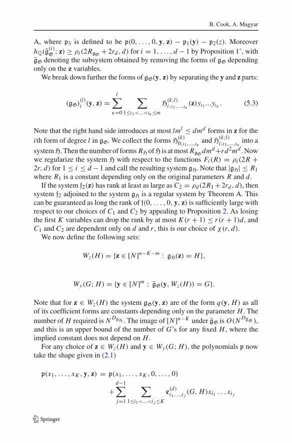
the choice of the (y, z) partition and there are crudely at most RG ≤ d2 K dr ≤dd+2rd+1 of them. By Proposition 1’, there is a system gG which is a strongregularization of G with respect to the functions Fi (R) = ρi (2R + 2rd , d)(i = 1, . . . , d−1) and the variables z so that the number of forms of degree i ingG is bounded in terms of r and d independently of the choice of the partitionof the variables. Correspondingly for any choice of the variables (y, z)we haveRgG ≤ R0 for an appropriate constant R0 = R0(r, d).

The variables y, and thus z as well, are now chosen by Proposition 2 withthe choice of C1 = 2d−1ρd(2R0 + 2rd , d) so that the forms

f(0, . . . , 0, y, z) = f1(y)+ g(y, z)+ f2(z)

have Bd(f1(y)+g(y, z)) ≥ C1 with the number of y variables, m, being at mostC1r . With this choice we have that the system obtained by adjoining eitherof the systems f1 + g or p1 + p3 to the gG is a regular system by Theorem

123

B. Cook, A. Magyar

A, where p3 is defined to be p(0, . . . , 0, y, z) − p1(y) − p2(z). MoreoverhQ(g

(i)G ; z) ≥ ρi (2RgG + 2rd , d) for i = 1, . . . , d − 1 by Proposition 1’, with

gG denoting the subsystem obtained by removing the forms of gG dependingonly on the z variables.

We break down further the forms of gG(y, z) by separating the y and z parts:

(gG)(l)i (y, z) =

l∑

κ=0

∑

1≤ι1<...<ικ≤m

H(k;l)i;ι1,...,ικ (z)yι1 ...yικ . (5.3)

Note that the right hand side introduces at most lml ≤ dmd forms in z for thei th form of degree l in gG. We collect the forms H

(k)0;ι1,...,ικ and H

(k;l)i;ι1,...,ικ into a

system H. Then the number of forms RH of H is at most RgGdmd+rd2md . Nowwe regularize the system H with respect to the functions Fi (R) = ρi (2R +2r, d) for 1 ≤ i ≤ d − 1 and call the resulting system gH. Note that |gH| ≤ R1where R1 is a constant depending only on the original parameters R and d.

If the system f2(z) has rank at least as large as C2 = ρd(2R1 +2rd , d), thensystem f2 adjoined to the system gH is a regular system by Theorem A. Thiscan be guaranteed as long the rank of f(0, . . . , 0, y, z) is sufficiently large withrespect to our choices of C1 and C2 by appealing to Proposition 2. As losingthe first K variables can drop the rank by at most K (r + 1) ≤ r(r + 1)d, andC1 and C2 are dependent only on d and r , this is our choice of χ(r, d).

We now define the following sets:

Wz(H) = {z ∈ [N ]n−K−m : gH(z) = H},

Wy(G; H) = {y ∈ [N ]m : gG(y,Wz(H)) = G}.

Note that for z ∈ Wz(H) the system gG(y, z) are of the form q(y, H) as allof its coefficient forms are constants depending only on the parameter H . Thenumber of H required is N DgH . The image of [N ]n−K under gG is O(N DgG ),and this is an upper bound of the number of G’s for any fixed H , where theimplied constant does not depend on H .

For any choice of z ∈ Wz(H) and y ∈ Wy(G; H), the polynomials p nowtake the shape given in (2.1)

p(x1, . . . , xK , y, z) = p(x1, . . . , xK , 0, . . . , 0)

+d−1∑

j=1

∑

1≤i1<...<i j ≤K

c(d)i1,...,i j(G, H)xi1 . . . xi j

123


+d−1∑

κ=1

∑

1≤ι1<...<ικ≤m

c(d)0;i1,...,i j(H)yι1 . . . yικ

+p1(0, . . . , 0, y, 0)+ p2(0, . . . , 0, 0, z)

:= P0(x1, . . . , xK ,G, H)+ P1(y, H)+ p2(z). (5.4)

Indeed on the level set Wz(H) the values of the forms gH and in turn thoseof the forms H are fixed, including the forms of gG depending only on the zvariables. Then for y ∈ Wy(G; H) the values of the forms gG and hence thevalues of the all forms in gG are fixed, which in turn fix the values of coefficientforms G. Define the exponential sums

S0(α,G, H) =∑

x1,...,xK ∈[N ]�(x1) . . . �(xK )e(α · P0(x1, . . . , xk,G, H)).

S1(α,G, H) =∑

y∈Wy(G;H)

�(y)e(α · P1(y, H)).

S2(α, H) =∑

z∈Wz(H)

�(z)e(α · p2(z)).

Now we have to bound the expression

EC(N ) =∑

H

∑

G

∫

m(C)

S0(α,G, H)S1(α,G, H)S2(α, H)e(−s · α)dα.

Proceeding as in Sect. 2.1, we obtain

(EC(N ))2 �

(

(log N )2n N DgG+DgH sup

H,G||S0(·,G, H)||2∞(m(C))

)

×∑

H

∑

G

||S1(·,G, H)||22||S2(·, H)||22 (5.5)

The summands on the right hand side can be expressed as the number ofsolutions of P1(y, H) = P1(y′, H) for y, y′ ∈ Wy(G; H) times the number ofsolutions to p2(z) = p2(z′) for z, z′ ∈ Wz(H). The conditions z, z′ ∈ Wz(H)may be replaced by the conditions z, z′ ∈ [N ](n−K−m) and gH(z) = gH(z′) =H . The conditions y, y′ ∈ W2(G; H) may be replaced by the conditionsy, y′ ∈ [N ]m and gG(y, z) = gG(y′, z) = G for any z ∈ Wz(H).

123

B. Cook, A. Magyar

In short, we are summing over all G and H the number of solutions to thesystem

P1(y, H) = P1(y′, H)

gG(y, z) = gG(y′, z) = G

p2(z) = p2(z′)gH(z) = gH(z′) = H

for y, y′ ∈ [N ]m and z, z′ ∈ [N ](n−K−m). With a little rearrangement thisbecomes

P1(y, gH(z)) = P1(y′, gH(z))

gG(y, gH(z)) = gG(y′, gH(z)) = G

p2(z) = p2(z′)gH(z) = gH(z′) = H,

and summing over G and H now simply removes two of the equalities. Andafter doing so, by removing gH as an argument puts us in the final form

p1(y)+ p3(y, z) = p1(y′)+ p3(y′, z)

gG(y, z) = gG(y′, z)

p2(z) = p2(z′) (5.6)

gH(z) = gH(z′),

for y, y′ ∈ [N ]m and z, z′ ∈ [N ](n−K−m). Let us call the number of solutionsto the system (5.6) W . Then (5.5) takes the form

(EC(N ))2 ≤ O

(

(log N )2nW N DgG+DgH sup

H,G||S0(·,G, H)||2∞(m(C))

)

.

(5.7)Proposition 3 follows immediately from the following two claims.

Claim 1: Given c>0, there is a C such that the bound

||S0(·,G, H)||∞(m(C)) = O((log N )−c N K ) (5.8)

holds uniformly in G and H.Claim 2: With the rank of p1(y) + p3(y, z) and p2(z) sufficiently large, thebound

W = O(

N 2(n−K )−2Dp−DgH−DgG

)(5.9)

holds.

123


Let us start with claim 1. We look at α · P0(x1, . . . , xK ,G, H), focusingon the coefficients of terms of the form xi1 ...xid for 1 ≤ i j ≤ K . From ourchoice of x1, . . . , xK , there is a collection of indices, say

(iκ1 , . . . , iκd

)for each

1 ≤ κ ≤ r , such that the collection {biκ1 ,...,iκd} is linearly independent. Let M

denote the r × r matrix of these coefficient vectors as rows. The coefficientof xiκ1

...xiκdin α · P0(x1, . . . , xK ,G, H) is (Mα)κ . Because M has full rank,

there is some term of the form xiκ1...xiκd

with a coefficient β where β ∈ m(C ′)for some slightly larger C ′.

If it happens to be the case that the indices iκ1 , . . . , iκd are equal, say all 1, thenthe bound follows directly from the bound in Lemma 5 for the x1 summation,and claim 1 follows by treating the other sums trivially. Otherwise we assumethat xiκ1

...xiκd= xγ1

1 ..., xγll where

∑γi = d and l < d. Now look at the sum

S0 in the form

∑

xl+1,...,xK ∈[N ]�(xl+1)...�(xK )

×∑

x1,...,xl∈[N ]�(x1)...�(xl)e(βxγ1

1 ...xγll + Q(x1, . . . , xK ,G, H))

where Q(x1, . . . , xK ,G, H) is viewed as a polynomial in x1, . . . , xl of degreeless than d with coefficients in the other xi and the G and the H . We proceedby using the Weyl differencing method, that is applying the Cauchy–Schwarzinequality γi times to the inner sum T0 for each of the variables xi . This givesthe upper bound

|T0|2d ≤ (log N )d2dN 2dl−d−l

∑

x1,...,xl

∑

w11,...,w

1γ1

...∑

wl1...w

1γl

×(

l∏

i=1

�wi1,...,w

iγl

1xi ∈[N ]

)

e(βw1

1...wlγl

),

where �w f (x) = f (x + w) f (x) is the multiplicative differencing operator,and�w1,w2 = �w2(�w1), and so on. For a fixed value of x-variables, the innersum is taken over a convex set K(x) ⊆ [−N , N ]d . Renaming the w-variablesas w = (w1, . . . , wd) and fixingw1, . . . , wd−1, the sum inwd is taken over aninterval of length at most 2N of a phase which is linear inwd and is estimated

by min(

2N , 1‖βw1...wd−1‖

). Here ‖γ ‖ denotes the distance of a real number

123

B. Cook, A. Magyar

γ to the nearest integer. Thus we have that

|T0|2d ≤ (log N )d2dN 2dl−d

×∑

(w1,...,wd−1)∈[−N ,N ]d−1

min

(2N ,

1

‖βw1 . . . wd−1‖).

At this point we proceed as in [2] Sec.2, see Lemmas 2.1–2.4, however as ourcontext is slightly different we briefly describe the argument below. First notethat by the multi-linearity of the expression in the denominator, we have thatthe sum in the w-variables is bounded by 2N log N -times the cardinality ofthe set

AN :={

w = (w1, . . . wd−1) ∈ [−N , N ]d−1; ‖βw1 . . . wd−1‖ ≤ 1

N

}.

For given 1 ≤ M < N define the sets

AN ,M :={

w = (w1, . . . wd−1) ∈[− N

M,

N

M

]d−1

;

‖βw1 . . . wd−1‖ ≤ 1

N Md−1

}

.

Applying Lemma 2.3 in [2]—a result from the geometry of numbers - succes-sively in the variables wi , we have that

|AN | � Md−1 |AN ,M |.Choose M := N (log N )−C ′′

with C ′′ = C ′/d, and notice if there is a vectorw = (w1, . . . , wd−1) ∈ AN ,M so that q := |w1 . . . wd−1| ≥ 1, then ‖qβ‖ ≤N−d (log N )C

′and hence β would be in the major arcs M(C ′) contradicting

our assumption. Thus all vectors w ∈ AN ,M have at least one zero coordinatewhich implies that |AN ,M | � (log N )(d−2)C ′′

, which gives the upper bound

|T0|2d � N 2dl (log N )d2d+1−C ′′ ≤ N 2dl (log N )−C ′′/2,

if C , and hence C ′ and C ′′, is chosen sufficiently large with respect to d. Claim1 follows by taking the 2d th root and summing trivially in xl+1, . . . , xK .

We turn to the proof of claim 2. One may write W =∑z T1(z)T2(z)where,for fixed z, T1(z) is the number of solutions y, y′ ∈ [N ]m to the system

p1(y)+ p3(y, z) = p1(y′)+ p3(y′, z)

gG(y, z) = gG(y′, z),

123


while T2(z) is the number of solutions z′ ∈ [N ]n−K−m to

p2(z) = p2(z′)gH(z) = gH(z′),

By the Cauchy–Schwarz inequality we have that W2 ≤ (∑z T1(z)2) (∑

z T2

(z)2) =: W1W2.

Now, W1 is the number of y, y′,u,u′ ∈ [N ]m and z ∈ [N ]n−K−m satisfyingthe equations

p1(y)+ p3(y, z)− p1(y′)− p3(y′, z) = 0

p1(u)+ p3(u, z)− p1(u′)− p3(u′, z) = 0

gG(y, z)− gG(y′, z) = 0, (5.10)

gG(u, z)− gG(u′, z) = 0,

and W2 is the number of z, z′, v′ ∈ [N ]n−K−m satisfying

p2(z)−p2(z′) = 0, p2(z)−p2(v′) = 0gH(z)−gH(z′) = 0, gH(z)−gH(v′) = 0(5.11)

First we consider the system in (5.10), and estimate the rank of the familyof degree d forms. For given λ,μ ∈ Q

r assume we have the decomposition

λ · (f1(y)+ g(y, z)− f1(y′)− g(y′, z))+ μ · (f1(u)

+g(u, z)− f1(u′)− g(u′, z)) =h∑

i=1

Ui Vi ,

where Ui (y, y′,u,u′, z) and Vi (y, y′,u,u′, z) are homogeneous forms of pos-itive degree. Using the facts that f1(0) = 0 and g(0, z) vanishes identically,substituting y′ = u = u′ = 0 gives

λ · (f1(y)+ g(y, z)) =h∑

i=1

U ′i (y, z)V ′

i (y, z),

thus h ≥ hQ(f1 + g) ≥ 21−dBd(f1 + g) ≥ ρd(2RgG + 2rd). Here we usedthe fact that hQ(f) ≥ hC(f) ≥ 21−dBd(f) for a homogeneous form f of degreed, see [17], Lemma 16.1. To estimate the rank of the degree i forms for given

123

B. Cook, A. Magyar

2 ≤ i ≤ d − 1 we invoke Lemma 2. We have that

hQ

((g(i)G (y, z)− g

(i)G (y

′, z), g(i)G (u, z)− g(i)G (u

′, z))

; z)

= hQ

(g(i)G (y, z)− g

(i)G (y

′, z); z)

≥≥ hQ

(g(i)G (y, z), g(i)G (y

′, z); z)

= hQ

(g(i)G (y, z); z

)≥ ρi

(2RgG + 2rd

)

Since hQ( f (y, z)) ≥ hQ( f (y, z); z) for any system of forms f and the totalnumber of forms of system (5.10) is 2RgG + 2rd , one has by Theorem A

W1 = O(

N 4m+n−K−m−2Dp−2DgG

).

For system (5.11) the estimates are simpler. Similarly as above it is easyto see directly from the definition that forms of this system of degree i haveSchmidt rank at least ρi (2RgH + 2rd , d). Indeed, suppose for λ,μ ∈ Q

r withsay λ �= 0

λ · (f2(z)− f2(z′))+ μ · (f2(z)− f2(v′)) =h∑

i=1

Ui (z, z′v, )Vi (z, z′v, ).

Substituting z′ = v′ = 0 we have λ · f2(z) = ∑hi=1 U ′

i (z) V ′i (z) and as not

all terms in the sum can be zero and for each non-zero term U ′i (z)V

′i (z) both

forms have positive degrees we have that h ≥ hQ(f2). The rank of the systemsg(i)H are estimated the same way. The system (5.11) hence

W2 = O(

N 3(n−K−m)−2Dp−2DgH

).

Putting these estimates together

W ≤ √W1W2 = O(

N 2(n−K )−2Dp−DgG−DgH

).

This proves claim 2 and Proposition 3 follows. ��

6 The major arcs

The treatment of the major arcs is fairly standard and differs little from thescenario with diagonal equations (see Hua [11]). Recall that the major arcsare a union of boxes of the form Ma,q(C), where q ≤ (log N )C and C isnow a fixed constant chosen large enough so that Lemma 3 holds with c = 1.

123


For a fixed a and q, the small size of the associated major arc means that theexponential sum

Tp(α) =∑

x∈[N ]n

�(x)e(p(x) · α)

can be replaced by any approximation that has a sufficiently large logarithmicpower gain in the error.

Upon the actual fixing of a q ≤ (log N )C and an a ∈ U nq , one has2

Tp(α) =∑

x∈[N ]n

�(x)e(p(x) · α)

=∑

g∈Znq

∑

x∈[N ]n

1x≡g (q)�(x)e(a · p(g)/q)e(p(x) · τ)

=∑

g∈Znq

e(p(g) · a/q)∫

X∈NJe(p(X) · τ)dψg(X), (6.1)

where the notations introduced here are τi = αi − ai/q, and ψg(X) =ψg1(X1)...ψgn (Xn) with

ψl(v) =∑

t≤v, t≡l (q)

�(t),

and J is the unit cube [0, 1]n ⊂ Rn .

Lemma 6 For any given a constant c, the estimate∫

X∈NJe(p(X)·τ)dψg(X)=1g∈U n

qφ(q)−n

∫

z∈NJe(p(z)·τ)dz+O((log N )−c N n)

(6.2)holds on each major arc Ma,q(C) provided that C is sufficiently large.

Proof Define for a fixed l the one dimensional signed measure dνl = dψl −dωl , where dωl is the Lebesgue measure multipled by the reciprocal of thetotient of q if l ∈ Uq , and is zero otherwise. For a continuous function f onethen has

N∫

0

f (X)dνl(X) =∑

x∈[N ], x≡l (q)

�(x) f (x)− φ(q)−1

N∫

0

f (z)dz.

2 There is some ambiguity in the case where N is a prime power, however, there is no harm inassuming that this is not so due to the fact that the prime powers are sparse.

123

B. Cook, A. Magyar

Now set d|νl | = dωl + dψl , so that

∫

X∈NJe(p(X) · τ)dψg(X) =

∫

X∈NJe(p(X) · τ)

n∏

i=1

(dνgi (Xi )+ dωgi (Xi )

).

Expanding out the product in the last integral gives the form

∫

X∈NJe(p(X) · τ)dωg(X)+

2n−1∑

i=1

∫

X∈NJe(p(X) · τ)dμi,g(X),

where dμi,g runs over all of the corresponding product measures, barring thedωg(X) term.

Consider ∫

X∈NJe(p(X) · τ)dμi,g(X)

for some fixed i . Assume without loss of generality that dμi,y is of the form

dνg1(X1)dσg(X2, . . . , Xn),

where dσg may be signed in some variables and is independent of g1. The rangeof integration for the X1 variable is a copy of the continuous interval [0, N ],and is to be split into smaller disjoint intervals of size N 1(log N )−c′

. Here c′is chosen to be between (c+C) and 2(c+C) such that (log N )c

′is an integer,

say B. The equality [0, N ] =⋃Bj=1 I j follows. Also set J ′

j = I j ×[0, N ]n−1,which absorbs the factor of N .

Now, for a fixed interval I j , select some t ∈ I j . Then write

∫

X∈J ′j

e(p(X) · τ )dμi,g =∫

X∈J ′j

e(p(t, X2, . . . , Xn) · τ)dνg1(X1)dσg(X2, . . . , Xn)

+∫

X∈B|

(e(p(X1, . . . , Xn) · τ)− e(p(t, X2, . . . , Xn) · τ))

×dνg1(X1)dσg(X2, . . . , Xn)

:= E1 + E2

The first error term satisfies

|E1| ≤∫

X2,...,Xn∈[0,N ]|∫

I j

dνg1(X1)| d|σg|(X2, . . . , Xn)= O(

N ne−c0√

log N)

123


for some positive constant c0 by the Siegel–Walfisz theorem, as q ≤ (log N )C .To bound E2, note that on I j the integrand is

O(|p(X1, . . . , Xn)− p(t, X2, . . . , Xn) · τ |) = O((log N )C−c′)

.

In turn,

|E2| = O((log N )C−c′))

∫

X∈J ′j

d|νg1 |(X1)d|σg|(X2, . . . , Xn)

= O(N n(log N )C−2c′)).

There are 2n −1 error terms on each interval, so summing over the (log N )c′

intervals completes the proof. ��The integral appearing in the last result has a quick reduction, namely

∫

NJe(p(X)τ )dX =

∫

NJe(f(X)τ )dX + O(N n−1+ε),

recalling that f is the highest degree part of p. Following along with the workof Birch, ∫

NJe(f(X)τ )dX = N n

∫

ζ∈Je(f(ζ ) · N 2τ)dζ,

is denoted by N nI(J , N dτ) in [2]. This function is independent of a and q.Thus the integral over any major arc yields the common integral

∫

|τ |≤(log N )C

I(J , N dτ)e(−s · τ)dτ.

With μ = N−ds, set

J (μ;�) =∫

|τ |≤�I(J , τ )e(−μ · τ)dτ,

andJ (μ) = lim

�→∞ J (μ;�).The following is Lemma 5.3 in [2].

123

B. Cook, A. Magyar

Lemma 7 The function J (μ) is continuous and uniformly bounded in μ.Moreover,

|J (μ)− J (μ,�)| � �− 12

holds uniformly in μ.

By definingWa,q =

∑

g∈U nq

e(p(g) · a/q),

one then has

Lemma 8 For any given c > 0, the estimate∫

Ma,q (C)

Tp(α)e(−s · α)dα = N n−drφ(q)−nWa,qe(−s · a/q)J (μ)

+O(N n−dr (log N )−c),

where μ = N−2s, holds on each major arc Ma,q(C).

The measure of the major arcs is easily at most N−dr (log N )K for someconstant K . By defining

B(s, q) =∑

a∈Urq

φ(q)−nWa,qe(−s · a/q)

S(s, N ) =∑

q≤(log N )C

B(s, q),

it then follows that

Lemma 9 The estimate

Mp,s(N ) = S(s, N )J (μ)N n−dr + O((log N )−c N n−dr ) (6.3)

holds for any chosen value of c.

7 The singular series

Following the outline of Hua ([11], chapter VIII, §2, Lemma 8.1), one can showthat B(s, q) is multiplicative as a function of q. This leads to consideration ofthe formal identity

S(s) := limN→∞ S(s, N ) =

∏

p<∞

(

1 +∞∑

t=1

B(s, pt )

)

. (7.1)

123


Lemma 10 If q = pt is a prime power, then

B(s, q) = O(

qr−B(p)/((d−1)2dr)+ε) (7.2)

holds uniformly in s as t → ∞. The implied constants can be made indepen-dent of p.

Proof It is shown here that

Wa,q = O(

qn−B(p)/((d−1)2dr)+ε) ,

uniformly for a ∈ U nq , which clearly implies the result by the definition of

B(s, q) and the fact that qn/φ(q)n ≤ 2n independent of p.The inclusion-exclusion principle is used to bound Wa,q when q = pt when

t ≤ d. Let such a t be fixed, and note that the characteristic function of Upt

decomposes as1Upt (x) = 1 −

∑

h∈Z pt−1

1x=hp.

Applying this in the definition gives

Wa,q =∑

g∈U nq

e(p(g) · a/q)

=∑

g∈Znq

n∏

i=1

⎛

⎜⎝1 −

∑

hi ∈Z pt−1

1gi =hi p

⎞

⎟⎠ e(p(g) · a/q)

=∑

I⊆[n](−1)|I |

∑

h∈Z |I |pt−1

∑

g∈Znq

FI (g; h)e(p(g) · a/q), (7.3)

whereFI (g; h) =

∏

i∈I

1gi =phi

for h ∈ Z |I |p . In other words, FI is the characteristic function of the set HI,h =

{g : gi = phi ∀ i ∈ I }.The sets I ⊆ [n] divided into two categories according to whether |I | ≤

B(p)/(r + 1) or not. If I is a set fitting into the latter category, then the trivial

123

B. Cook, A. Magyar

estimate is

∣∣∣∣∣∣∣∣

∑

h∈Z |I |pt−1

∑

g∈Znq

FI (g; h)e(p(g) · a/q)

∣∣∣∣∣∣∣∣

= p(t−1)|I |(pt )n−|I |

= (pt )n−|I |/t ≤ qn−B(p)/(tr+t) ≤ qn−B(p)/((d−1)2dr).

Now let I be a fixed subset of [n] with |I | ≤ B(p)/(r + 1). For each h therestriction of p to the set HI,h has Birch rank at least B(p) − |I |(r + 1) bycorollary 4. By the work of Birch ([2], Lemma 5.4) it follows that

∑

h∈Z (t−1)|I |p

∣∣∣∣∣∣

∑

g∈Znq

FI (g; h)e(p(g) · a/q)

∣∣∣∣∣∣

� q(t−1)|I |/t qn−|I |−(B(p)−|I |(r+1))/((d−1)2d−1r)+ε

� qn−B(p)/((d−1)2dr)+ε.

Summing over all I yields the bound.Now let q = pt for t > d. Going back to the definition gives

Wa,q =∑

g∈U nq

e(p(g) · a/q)

=∑

g∈U np

∑

h∈Znpt−1

e(p(g + ph) · a/q).

The system of forms in the exponent can be expanded for each fixed g as

p(g + ph) = pdp(h)+ fg(h)

for some polynomial fg of degree at most d − 1. Then it follows that

|Wa,q | ≤∑

g∈U np

∣∣∣∣∣∣∣

∑

h∈Znpt−1

e( fg(h)+ pdp(h)) · a/q)

∣∣∣∣∣∣∣. (7.4)

The inner sum is now bounded uniformly in g by an application of theexponential sum estimates in [2] as follows.

123


Set P = pt−1 and q1 = pt−d . Then, for each i = 1, . . . , r ,

2|q ′ai − a′i q1| ≤ P−(d−1)+(d−1)rθ

and1 ≤ q ′ ≤ P(d−1)rθ

cannot be satisfied if θ < 1/(d − 1)r . Then, by Lemma 4.3 of [2],

∑

h∈Znpt−1

e((pdp(h)) · a/q + f (h)) = O(Pn−B(p)/((d−1)2dr)+ε)

for any polynomial f (h) of degree strictly less than d. In turn,

|Wa,q | ≤∑

g∈U np

O(Pn−B(p)/((d−1)2dr)+ε) = O(qn−B(p)/((d−1)2dr)+ε),

which is what is needed to complete the proof in this last and final case. ��Now define the local factor for a finite prime p as

μp = 1 +∞∑

t=1

B(s, pt )), (7.5)

which is well defined as the series is absolutely convergent provided thatB(p) > (d − 1)2dr(r + 1). The following result is again an straight forwardextension of the results for a single form.

Lemma 11 For each finite prime p, the local factor may be represented as

μp = limt→∞

(pt )R M(pt )

φn(pt ), (7.6)

where M(pt ) represents the number of solutions to Eq. 2.2 in the multiplicativegroup Upt .

At our disposal now is the fact that the μp are positive, which then easilygives the following.

Lemma 12 If B(p) > (d − 1)2dr(r + 1) then the local factor for each finiteprime satisfies the estimate

μp = 1 + O(p−(1+δ))

for some positive δ, and therefore the product in Eq. 7.1 is absolutely convergentand thusly is in fact well defined.

123

B. Cook, A. Magyar

The observation that

|S(s, N )− S(s)| = o(1)

gives the final form of the asymptotic

Mp,s(N ) = S(s)J (μ)N n−dr + O((log N )−c N n−dr ).

This proves our main result, Theorem 1. The non-vanishing of local factorsfollows from the exact same lifting argument as when dealing with integersolutions [2].

8 Further remarks

There are further possible refinements of the main result of this paper. It isexpected, similarly to the case of integer solutions [17], that Theorem 1 holdsassuming only the largeness of the rational Schmidt rank of the system. Toprove this one needs to find a suitable analogue of Proposition 2 for the rationalSchmidt rank instead of the Birch rank. The tower type bounds on the ranksare due to the regularization process expressed in Proposition 1. It is expectedthat exponential type lower bounds on the rank of the system are sufficient. Itmight be possible that there are “transfer principles” for higher degree forms,to allow a more direct transition to find solutions in the primes.

The methods of this paper may extend to other special sequences not justthe primes. For example for a translation invariant system of forms one mightmodify our arguments to show the existence of solutions chosen from a set Aof upper positive density. Indeed, assuming that A is sufficiently uniform, oneexpects that an analogue of Lemma 5 and hence our main estimate Proposi-tion 3 holds, with the minor arcs replaced by [0, 1]r . Otherwise the balancedfunction of A should correlate with a polynomial phase function which natu-rally leads to a standard density increment argument. Note that the existenceof solutions in the set A already follows from known results, Szemerédi’s the-orem [8] together with the main result of Birch [2], providing though weakerquantitative bounds on the density. We do not pursue these matters here.

References

1. Balog, A.: Linear equations in primes. Mathematika 39(2), 367–378 (1992)2. Birch, B.: Forms in many variables. Proc. Royal Soc. Lond. Ser. A. 265(1321), 245–263

(1962)3. Bourgain, J., Gamburd, A., Sarnak, P.: Afne linear sieve, expanders, and sum-product.

Invent. Math. 179, 559644 (2010)

123


4. Brdern, J., Dietmann, J., Liu, J., Wooley, T.: A Birch–Goldbach theorem. Archiv der Math-ematik 94(1), 53–58 (2010)

5. Goldston, D., Pintz, J.: Yildirim, Primes in tuples I. Ann. Math. 170, 819–862 (2009)6. Golsefidy, A.S., Sarnak, P.: The affine sieve. J. Am. Math. Soc. 26(4), 1085–1105 (2013)7. Green, B., Tao, T.: Linear equations in the primes. Ann. Math. (2) 171(3), 1753–1850

(2010)8. Green, B., Tao, T.: Yet another proof of Szemerédi’s theorem. An irregular mind, pp. 335–

342. Springer, Berlin Heidelberg, (2010)9. Green, B., Tao, T.: The distribution of polynomials over finite fields, with applications to

the Gowers Norms. Contrib. Discret. Math. 4, 1–36 (2009)10. Hartshorne, R.: Algebraic geometry, Graduate Texts in Mathematics, vol. 52. Springer,

Verlag (1977)11. Hua, L.K.: Additive theory of prime numbers, Translations of Mathematical Monographs,

vol. 13”. Am. Math. Soc., Providence (1965)12. Kaufman, T., Lovett, S.: Worst case to average case reductions for polynomials. In: 49th

Annual IEEE Symposium on Foundations of Computer, Science, pp. 166–175, (2008)13. Keil, E.: Translation invariant quadratic forms in dense variables, preprint14. Liu, J., Sarnak, P.: Integral points on quadrics in three variables whose coordinates have

few prime factors. Israel J. Math. 178, 393–426 (2010)15. Liu, J.: Integral points on quadrics with prime coordinates. Monats. Math. 164(4), 439–465

(2011)16. Duke, W., Rudnick, Z., Sarnak, P.: Density of integer points on affine homogeneous vari-

eties. Duke Math. J. 71(1), 143–179 (1993)17. Schmidt, W.: The density of integral points on homogeneous varieties. Acta. Math. 154(3),

243–296 (1985)18. Vinogradov, I.M.: Representations of an odd integer as a sum of three primes Goldbach

Conjecture 4, 61 (2002)19. Zhang, Y.:Bounded gaps between primes. Ann. Math., to appear

123

Documents

Diophantine equations in the primes