Embed Size (px)
Citation preview
Diophantine equations Cubic equations FLT Pell’s equation Elliptic curves Back to FLT
Diophantine equations
Henri Darmon
McGill University
CRM-ISM Colloquium, UQAM, January 8, 2010
Diophantine equations Cubic equations FLT Pell’s equation Elliptic curves Back to FLT
1 Diophantine equations
2 Cubic equations
3 FLT
4 Pell’s equation
5 Elliptic curves
6 Back to FLT
Diophantine equations Cubic equations FLT Pell’s equation Elliptic curves Back to FLT
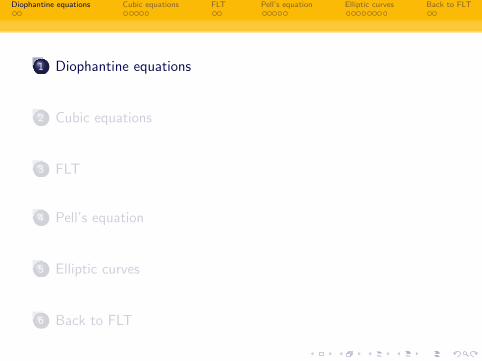
Definition
A Diophantine equation is a system of polynomial equations withinteger coefficients:
f1(x1, . . . , xm) = · · · = fn(x1, . . . , xm) = 0,
in which one is solely interested in the integer solutions.
Some examples:
1 Cubic equations, like y2 = x3 + 1;
2 The Fermat-Pell equation: x2 − Dy2 = 1;
3 Fermat’s equation: xn + yn = zn;
4 x19y3 − 198z713 + 15xyz3 = 1098w2001.
A large part of number theory is concerned with the study ofDiophantine equations.
Diophantine equations Cubic equations FLT Pell’s equation Elliptic curves Back to FLT
Some questions a number theorist might be asked
This is the 21st century. Are there still questions about wholenumbers that we don’t know how to answer?
Isn’t the study of Diophantine equations just a recreationalpursuit?
Claim: Diophantine equations lie beyond the realm of recreationalmathematics, because their study draws on a rich panoply ofmathematical ideas. These ideas, and the new questions they leadto, are just as interesting (perhaps more!) than the equationswhich might have led to their discovery.
Diophantine equations Cubic equations FLT Pell’s equation Elliptic curves Back to FLT
1 Diophantine equations
2 Cubic equations
3 FLT
4 Pell’s equation
5 Elliptic curves
6 Back to FLT
Diophantine equations Cubic equations FLT Pell’s equation Elliptic curves Back to FLT
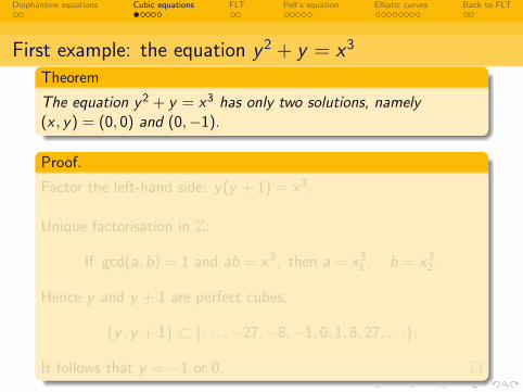
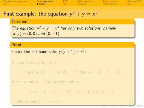
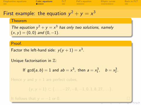
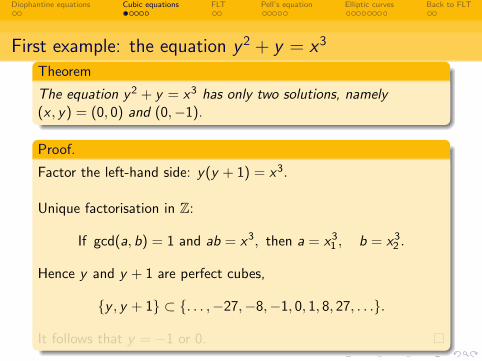
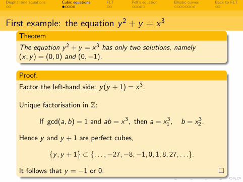
First example: the equation y 2 + y = x3
Theorem
The equation y2 + y = x3 has only two solutions, namely(x , y) = (0, 0) and (0,−1).
Proof.
Factor the left-hand side: y(y + 1) = x3.
Unique factorisation in Z:
If gcd(a, b) = 1 and ab = x3, then a = x31 , b = x3
2 .
Hence y and y + 1 are perfect cubes,
{y , y + 1} ⊂ {. . . ,−27,−8,−1, 0, 1, 8, 27, . . .}.
It follows that y = −1 or 0.
Diophantine equations Cubic equations FLT Pell’s equation Elliptic curves Back to FLT
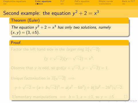
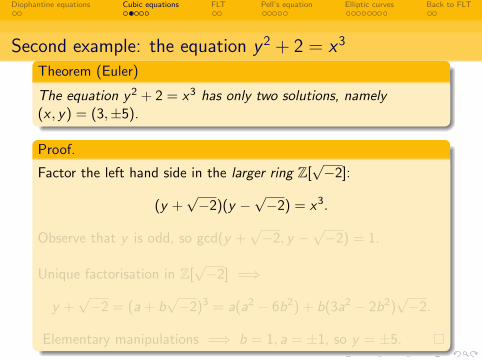
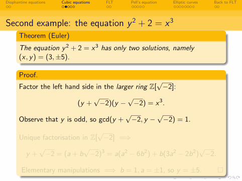
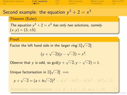
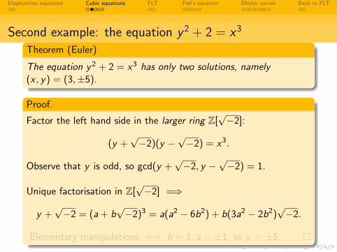
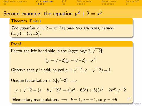
Second example: the equation y 2 + 2 = x3
Theorem (Euler)
The equation y2 + 2 = x3 has only two solutions, namely(x , y) = (3,±5).
Proof.
Factor the left hand side in the larger ring Z[√−2]:
(y +√−2)(y −
√−2) = x3.
Observe that y is odd, so gcd(y +√−2, y −
√−2) = 1.
Unique factorisation in Z[√−2] =⇒
y +√−2 = (a + b
√−2)3 = a(a2 − 6b2) + b(3a2 − 2b2)
√−2.
Elementary manipulations =⇒ b = 1, a = ±1, so y = ±5.
Diophantine equations Cubic equations FLT Pell’s equation Elliptic curves Back to FLT
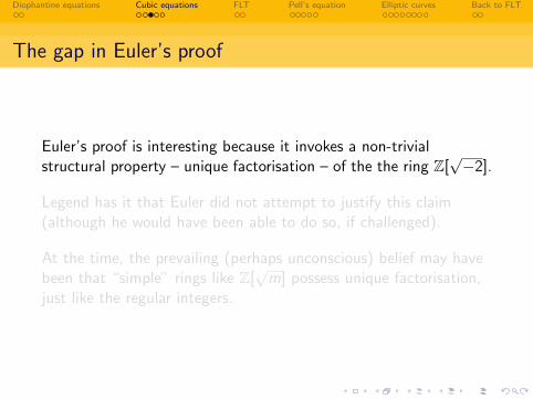
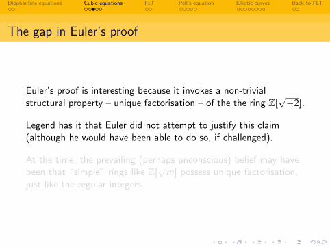
The gap in Euler’s proof
Euler’s proof is interesting because it invokes a non-trivialstructural property – unique factorisation – of the the ring Z[
√−2].
Legend has it that Euler did not attempt to justify this claim(although he would have been able to do so, if challenged).
At the time, the prevailing (perhaps unconscious) belief may havebeen that “simple” rings like Z[
√m] possess unique factorisation,
just like the regular integers.
Diophantine equations Cubic equations FLT Pell’s equation Elliptic curves Back to FLT
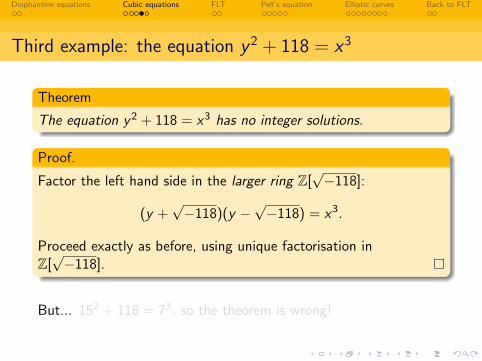
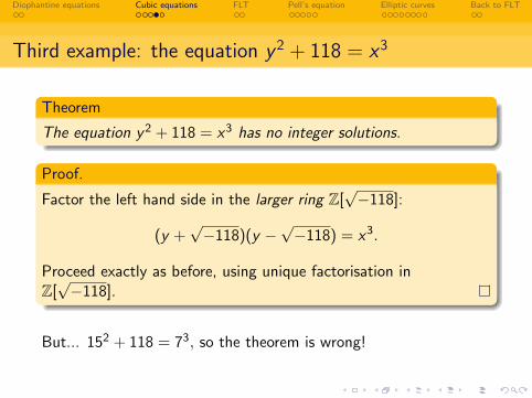
Third example: the equation y 2 + 118 = x3
Theorem
The equation y2 + 118 = x3 has no integer solutions.
Proof.
Factor the left hand side in the larger ring Z[√−118]:
(y +√−118)(y −
√−118) = x3.
Proceed exactly as before, using unique factorisation inZ[√−118].
But... 152 + 118 = 73, so the theorem is wrong!
Diophantine equations Cubic equations FLT Pell’s equation Elliptic curves Back to FLT
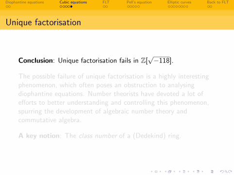
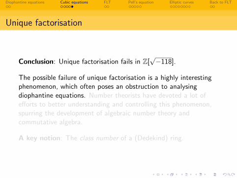
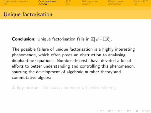
Unique factorisation
Conclusion: Unique factorisation fails in Z[√−118].
The possible failure of unique factorisation is a highly interestingphenomenon, which often poses an obstruction to analysingdiophantine equations. Number theorists have devoted a lot ofefforts to better understanding and controlling this phenomenon,spurring the development of algebraic number theory andcommutative algebra.
A key notion: The class number of a (Dedekind) ring.
Diophantine equations Cubic equations FLT Pell’s equation Elliptic curves Back to FLT
1 Diophantine equations
2 Cubic equations
3 FLT
4 Pell’s equation
5 Elliptic curves
6 Back to FLT
Diophantine equations Cubic equations FLT Pell’s equation Elliptic curves Back to FLT
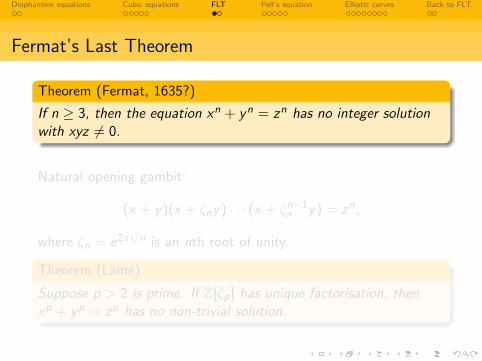
Fermat’s Last Theorem
Theorem (Fermat, 1635?)
If n ≥ 3, then the equation xn + yn = zn has no integer solutionwith xyz 6= 0.
Natural opening gambit:
(x + y)(x + ζny) · · · (x + ζn−1n y) = zn,
where ζn = e2πi/n is an nth root of unity.
Theorem (Lame)
Suppose p > 2 is prime. If Z[ζp] has unique factorisation, thenxp + yp = zp has no non-trivial solution.
Diophantine equations Cubic equations FLT Pell’s equation Elliptic curves Back to FLT
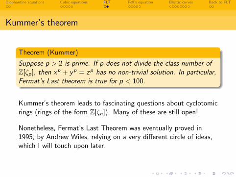
Kummer’s theorem
Theorem (Kummer)
Suppose p > 2 is prime. If p does not divide the class number ofZ[ζp], then xp + yp = zp has no non-trivial solution. In particular,Fermat’s Last theorem is true for p < 100.
Kummer’s theorem leads to fascinating questions about cyclotomicrings (rings of the form Z[ζn]). Many of these are still open!
Nonetheless, Fermat’s Last Theorem was eventually proved in1995, by Andrew Wiles, relying on a very different circle of ideas,which I will touch upon later.
Diophantine equations Cubic equations FLT Pell’s equation Elliptic curves Back to FLT
1 Diophantine equations
2 Cubic equations
3 FLT
4 Pell’s equation
5 Elliptic curves
6 Back to FLT
Diophantine equations Cubic equations FLT Pell’s equation Elliptic curves Back to FLT
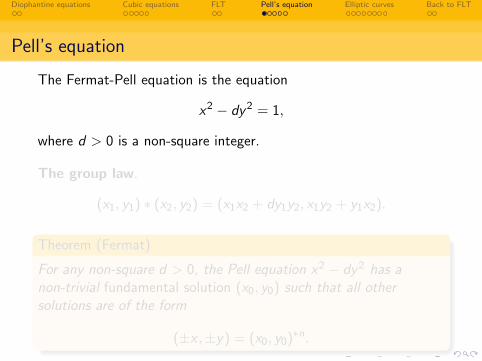
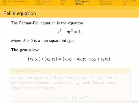
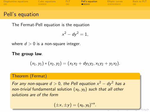
Pell’s equation
The Fermat-Pell equation is the equation
x2 − dy2 = 1,
where d > 0 is a non-square integer.
The group law.
(x1, y1) ∗ (x2, y2) = (x1x2 + dy1y2, x1y2 + y1x2).
Theorem (Fermat)
For any non-square d > 0, the Pell equation x2 − dy2 has anon-trivial fundamental solution (x0, y0) such that all othersolutions are of the form
(±x ,±y) = (x0, y0)∗n.
Diophantine equations Cubic equations FLT Pell’s equation Elliptic curves Back to FLT
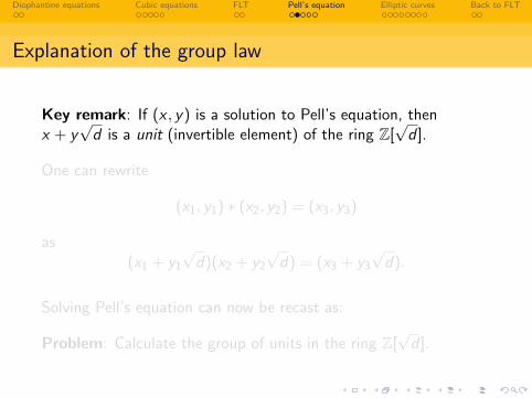
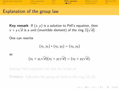
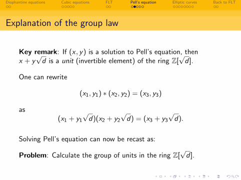
Explanation of the group law
Key remark: If (x , y) is a solution to Pell’s equation, thenx + y
√d is a unit (invertible element) of the ring Z[
√d ].
One can rewrite
(x1, y1) ∗ (x2, y2) = (x3, y3)
as(x1 + y1
√d)(x2 + y2
√d) = (x3 + y3
√d).
Solving Pell’s equation can now be recast as:
Problem: Calculate the group of units in the ring Z[√
d ].
Diophantine equations Cubic equations FLT Pell’s equation Elliptic curves Back to FLT
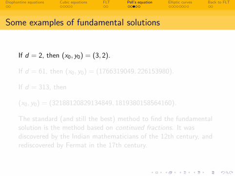
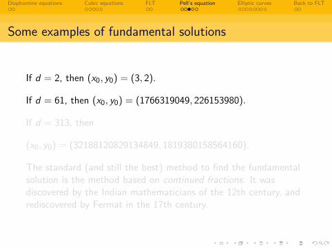
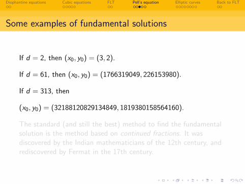
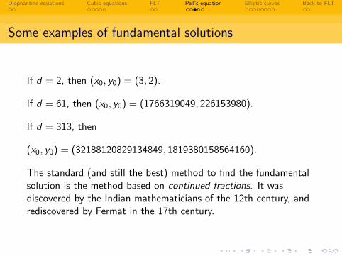
Some examples of fundamental solutions
If d = 2, then (x0, y0) = (3, 2).
If d = 61, then (x0, y0) = (1766319049, 226153980).
If d = 313, then
(x0, y0) = (32188120829134849, 1819380158564160).
The standard (and still the best) method to find the fundamentalsolution is the method based on continued fractions. It wasdiscovered by the Indian mathematicians of the 12th century, andrediscovered by Fermat in the 17th century.
Diophantine equations Cubic equations FLT Pell’s equation Elliptic curves Back to FLT
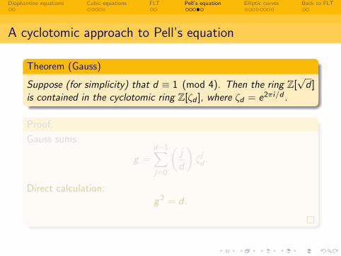
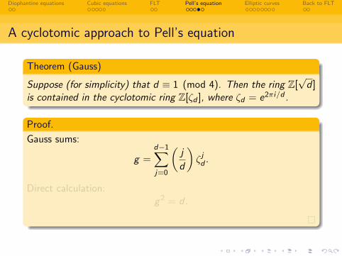
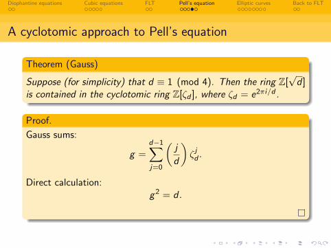
A cyclotomic approach to Pell’s equation
Theorem (Gauss)
Suppose (for simplicity) that d ≡ 1 (mod 4). Then the ring Z[√
d ]is contained in the cyclotomic ring Z[ζd ], where ζd = e2πi/d .
Proof.
Gauss sums:
g =d−1∑j=0
(j
d
)ζ jd .
Direct calculation:g2 = d .
Diophantine equations Cubic equations FLT Pell’s equation Elliptic curves Back to FLT
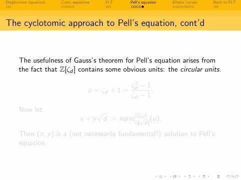
The cyclotomic approach to Pell’s equation, cont’d
The usefulness of Gauss’s theorem for Pell’s equation arises fromthe fact that Z[ζd ] contains some obvious units: the circular units.
u = ζd + 1 =ζ2d − 1
ζd − 1.
Now letx + y
√d := norm
Z[ζd ]
Z[√
d ](u).
Then (x , y) is a (not necessarily fundamental!) solution to Pell’sequation.
Diophantine equations Cubic equations FLT Pell’s equation Elliptic curves Back to FLT
1 Diophantine equations
2 Cubic equations
3 FLT
4 Pell’s equation
5 Elliptic curves
6 Back to FLT
Diophantine equations Cubic equations FLT Pell’s equation Elliptic curves Back to FLT
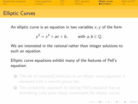
Elliptic Curves
An elliptic curve is an equation in two variables x , y of the form
y2 = x3 + ax + b, with a, b ∈ Q.
We are interested in the rational rather than integer solutions tosuch an equation.
Elliptic curve equations exhibit many of the features of Pell’sequation:
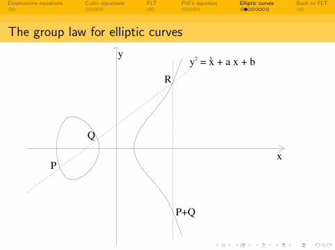
1 The set of (rational) solutions to an elliptic curve equation isequipped with a natural group law;
2 The cyclotomic approach to solving Pell’s equation has aninteresting (and quite deep) counterpart for elliptic curves.
Diophantine equations Cubic equations FLT Pell’s equation Elliptic curves Back to FLT
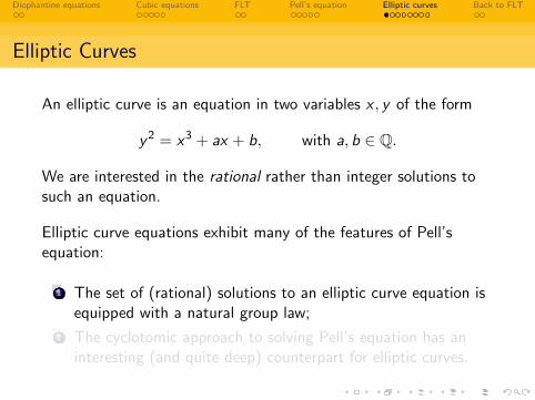
Elliptic Curves
An elliptic curve is an equation in two variables x , y of the form
y2 = x3 + ax + b, with a, b ∈ Q.
We are interested in the rational rather than integer solutions tosuch an equation.
Elliptic curve equations exhibit many of the features of Pell’sequation:
1 The set of (rational) solutions to an elliptic curve equation isequipped with a natural group law;
2 The cyclotomic approach to solving Pell’s equation has aninteresting (and quite deep) counterpart for elliptic curves.
Diophantine equations Cubic equations FLT Pell’s equation Elliptic curves Back to FLT
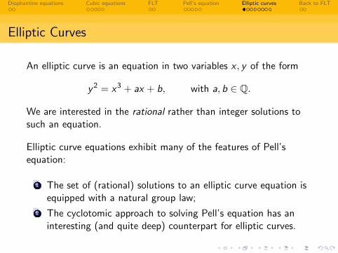
Elliptic Curves
An elliptic curve is an equation in two variables x , y of the form
y2 = x3 + ax + b, with a, b ∈ Q.
We are interested in the rational rather than integer solutions tosuch an equation.
Elliptic curve equations exhibit many of the features of Pell’sequation:
1 The set of (rational) solutions to an elliptic curve equation isequipped with a natural group law;
2 The cyclotomic approach to solving Pell’s equation has aninteresting (and quite deep) counterpart for elliptic curves.
Diophantine equations Cubic equations FLT Pell’s equation Elliptic curves Back to FLT
The group law for elliptic curves
x
y y = x + a x + b2 3
P
Q
R
P+Q
Diophantine equations Cubic equations FLT Pell’s equation Elliptic curves Back to FLT
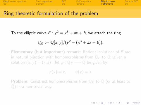
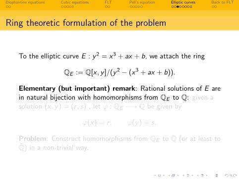
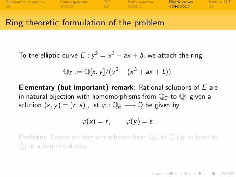
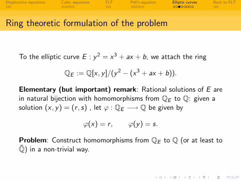
Ring theoretic formulation of the problem
To the elliptic curve E : y2 = x3 + ax + b, we attach the ring
QE := Q[x , y ]/(y2 − (x3 + ax + b)).
Elementary (but important) remark: Rational solutions of E arein natural bijection with homomorphisms from QE to Q: given asolution (x , y) = (r , s) , let ϕ : QE −→ Q be given by
ϕ(x) = r , ϕ(y) = s.
Problem: Construct homomorphisms from QE to Q (or at least toQ) in a non-trivial way.
Diophantine equations Cubic equations FLT Pell’s equation Elliptic curves Back to FLT
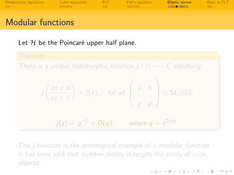
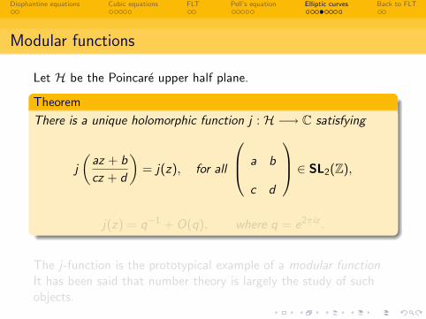
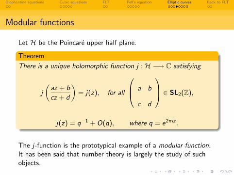
Modular functions
Let H be the Poincare upper half plane.
Theorem
There is a unique holomorphic function j : H −→ C satisfying
j
(az + b
cz + d
)= j(z), for all
a b
c d
∈ SL2(Z),
j(z) = q−1 + O(q), where q = e2πiz .
The j-function is the prototypical example of a modular function.It has been said that number theory is largely the study of suchobjects.
Diophantine equations Cubic equations FLT Pell’s equation Elliptic curves Back to FLT
Modular functions
Let H be the Poincare upper half plane.
Theorem
There is a unique holomorphic function j : H −→ C satisfying
j
(az + b
cz + d
)= j(z), for all
a b
c d
∈ SL2(Z),
j(z) = q−1 + O(q), where q = e2πiz .
The j-function is the prototypical example of a modular function.It has been said that number theory is largely the study of suchobjects.
Diophantine equations Cubic equations FLT Pell’s equation Elliptic curves Back to FLT
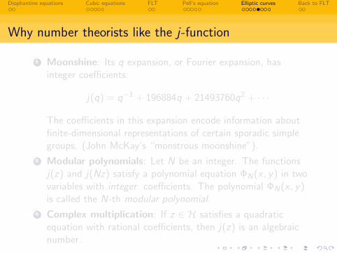
Why number theorists like the j-function
1 Moonshine: Its q expansion, or Fourier expansion, hasinteger coefficients:
j(q) = q−1 + 196884q + 21493760q2 + · · ·
The coefficients in this expansion encode information aboutfinite-dimensional representations of certain sporadic simplegroups. (John McKay’s “monstrous moonshine”).
2 Modular polynomials: Let N be an integer. The functionsj(z) and j(Nz) satisfy a polynomial equation ΦN(x , y) in twovariables with integer coefficients. The polynomial ΦN(x , y)is called the N-th modular polynomial.
3 Complex multiplication: If z ∈ H satisfies a quadraticequation with rational coefficients, then j(z) is an algebraicnumber.
Diophantine equations Cubic equations FLT Pell’s equation Elliptic curves Back to FLT
Modular rings
Using the modular polynomial ΦN(x , y), we can associate to eachN a ring of modular functions
QN := Q[x , y ]/(ΦN(x , y)) = Q(j(z), j(Nz)).
The ring QN will be called the modular ring of level N. Modularrings play the same role in the study of elliptic curves ascyclotomic rings in the study of Pell’s equation.
Diophantine equations Cubic equations FLT Pell’s equation Elliptic curves Back to FLT
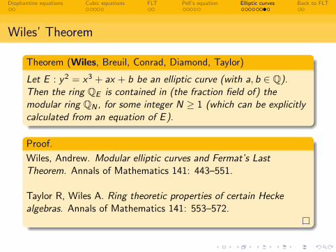
Wiles’ Theorem
Theorem (Wiles, Breuil, Conrad, Diamond, Taylor)
Let E : y2 = x3 + ax + b be an elliptic curve (with a, b ∈ Q).Then the ring QE is contained in (the fraction field of) themodular ring QN , for some integer N ≥ 1 (which can be explicitlycalculated from an equation of E ).
Proof.
Wiles, Andrew. Modular elliptic curves and Fermat’s LastTheorem. Annals of Mathematics 141: 443–551.
Taylor R, Wiles A. Ring theoretic properties of certain Heckealgebras. Annals of Mathematics 141: 553–572.
Diophantine equations Cubic equations FLT Pell’s equation Elliptic curves Back to FLT
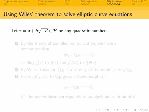
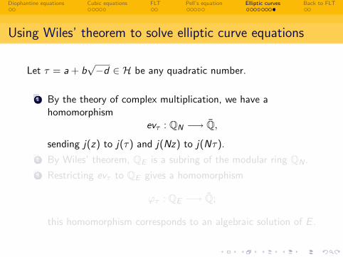
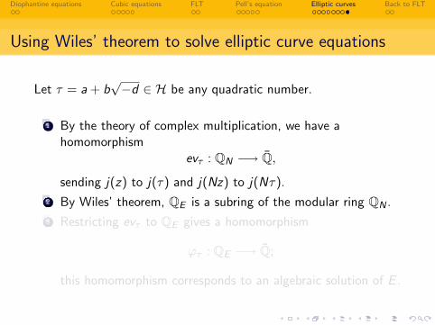
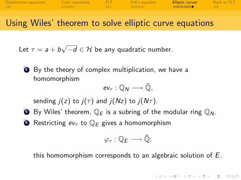
Using Wiles’ theorem to solve elliptic curve equations
Let τ = a + b√−d ∈ H be any quadratic number.
1 By the theory of complex multiplication, we have ahomomorphism
evτ : QN −→ Q,
sending j(z) to j(τ) and j(Nz) to j(Nτ).
2 By Wiles’ theorem, QE is a subring of the modular ring QN .
3 Restricting evτ to QE gives a homomorphism
ϕτ : QE −→ Q;
this homomorphism corresponds to an algebraic solution of E .
Diophantine equations Cubic equations FLT Pell’s equation Elliptic curves Back to FLT
1 Diophantine equations
2 Cubic equations
3 FLT
4 Pell’s equation
5 Elliptic curves
6 Back to FLT
Diophantine equations Cubic equations FLT Pell’s equation Elliptic curves Back to FLT
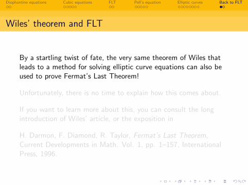
Wiles’ theorem and FLT
By a startling twist of fate, the very same theorem of Wiles thatleads to a method for solving elliptic curve equations can also beused to prove Fermat’s Last Theorem!
Unfortunately, there is no time to explain how this comes about.
If you want to learn more about this, you can consult the longintroduction of Wiles’ article, or the exposition in
H. Darmon, F. Diamond, R. Taylor, Fermat’s Last Theorem,Current Developments in Math. Vol. 1, pp. 1–157, InternationalPress, 1996.
Diophantine equations Cubic equations FLT Pell’s equation Elliptic curves Back to FLT
Better yet, come to Montreal and study number theory!