Embed Size (px)
Citation preview

DISCUSSION PAPER SERIES
IZA DP No. 12379
Robert A. Hart
Labor Productivity during the Great Depression in UK Manufacturing
MAY 2019

Any opinions expressed in this paper are those of the author(s) and not those of IZA. Research published in this series may include views on policy, but IZA takes no institutional policy positions. The IZA research network is committed to the IZA Guiding Principles of Research Integrity.The IZA Institute of Labor Economics is an independent economic research institute that conducts research in labor economics and offers evidence-based policy advice on labor market issues. Supported by the Deutsche Post Foundation, IZA runs the world’s largest network of economists, whose research aims to provide answers to the global labor market challenges of our time. Our key objective is to build bridges between academic research, policymakers and society.IZA Discussion Papers often represent preliminary work and are circulated to encourage discussion. Citation of such a paper should account for its provisional character. A revised version may be available directly from the author.
Schaumburg-Lippe-Straße 5–953113 Bonn, Germany
Phone: +49-228-3894-0Email: [email protected] www.iza.org
IZA – Institute of Labor Economics
DISCUSSION PAPER SERIES
ISSN: 2365-9793
IZA DP No. 12379
Labor Productivity during the Great Depression in UK Manufacturing
MAY 2019
Robert A. HartUniversity of Stirling and IZA
ABSTRACT
IZA DP No. 12379 MAY 2019
Labor Productivity during the Great Depression in UK Manufacturing*
This paper provides estimates of labor productivity for one-third of UK manufacturing
during the Great Depression. It covers engineering and allied industries, and metal working
industries. A unique data set of actual hours of work is combined with comparable
real output and employment statistics. It establishes that output per worker-hour was
countercyclical in the 1929-1932 peak-to-trough years of the Depression. This result has
also been found for US manufacturing over the same period. Working time is found to play
a crucial role the UK productivity response. Countercyclical productivity is discussed in terms
of (i) the strong final output and consumer price deflations of 1929 to 1934, (ii) an absence
of significant labor hoarding, and (c) diminishing returns to long weekly hours of work.
JEL Classification: O47, E32, N64
Keywords: labor productivity, Great Depression, diminishing returns to hours
Corresponding author:Robert A. HartDivision of EconomicsUniversity of StirlingStirling FK9 4LAUnited Kingdom
E-mail: [email protected]
* I thank Olaf Hübler and John Pencavel for helpful comments.

2
1. Introduction
Since the 1997/8 financial crisis, the most important UK labor market issue has
concerned the ‘productivity puzzle’ relating to a prolonged fall in labor productivity. Six
years after the onset of the crisis, productivity per hour was still 16% below its pre-crisis
trend growth path (Barnett et al. 2014). The Great Recession marked the severest economic
downturn since the Great Depression. Based on one-third of UK manufacturing industry, this
paper investigates the behavior of labor productivity during the Great Depression. The
contrast with recent experience is stark. I find that between 1929 and 1932, the peak-to-
trough years of the Depression cycle, labor productivity rose above and remained above its
initial peak. Output per worker-hour was countercyclical, a finding in line with US
manufacturing evidence over the same period (Bordo and Evans, 1993).
Analysis of UK labor in the inter-war years has been hampered by a scarcity of
adequate statistical background. This is principally due to a lack of data on actual hours of
work. The analysis here provides two interrelated advances. First, it makes use of a unique
data set of payroll records that provide detailed coverage of actual weekly hours worked by
timeworkers and pieceworkers. The records were compiled by member firms of the UK’s
largest manufacturing employers’ organisation, the Engineering Employers’ Federation
(EEF). These data are the best inter-war source of hours statistics in the UK.1 Second, it
establishes that changes in actual working time during the Great Depression were
fundatmentally important to the finding of countercyclical labor productivity.
The manufacturing activities of EEF member firms belong to the official industrial
classifications, Engineering and Allied Industries, and Metal Working Industries. The
1 The annual EEF payroll data cover the period 1914 to 1968.The current author and J. Elizabeth Roberts have assembled the complete data. See the UK Data Archive: (http://www.esds.ac.uk/findingData/snDescription.asp?sn=5569)
3
industries include iron foundries, iron and steel forgings, agricultural machinery, aircraft
manufacture, car and commercial vehicle production, boilers and boilerhouse plant,
construction engineering, electrical engineering, marine engineering, general engineering,
and machine tool manufacture. In order to derive measures of labor productivity, the hours
statistics are matched with published data on real output and employment for the same
industries.
I discuss three contributory factors that help to explain the productivity findings.
These are (i) a prevailing UK deflationary climate that were conducive to major reductions in
weekly hours from both demand and supply perspectives, (ii) a low propensity among
employers to hoard labor, and (iii) the likelihood that working time reductions entailed
increasing returns to hours.
The core analysis covers the critical years of the Great Depression cycle, from 1929 to
1935. In the sections dealing with the construction of the actual weekly hours measures
(Section 3) and with discussion of the subsequent labor productivity outcomes (Section 6),
the period is extended to the years 1927 to 1937 so as to include additional relevant
information.
2. Hours of work and labor productivity
There are two predominant measures of labor productivity, output per worker and
output per worker-hour. I begin by noting the difference between them. Let output per
worker be denoted Q1 = X/E, where X is output and E is employment. Let output per worker-
hour be given by Q2 = X/H, where H = E.h, the product of employment and average weekly
hours per worker. The proportionate (or log) change in Q1 is ΔQ1 = ΔX - ΔE. Similarly, ΔQ2
= ΔX - ΔE - Δh. The differences between the two productivity measures is ΔQ2 - ΔQ1 = -
Δh, or the negative of the proportionate change in average per worker weekly hours. I show
4
that the change in average weekly hours plays an essential role in determining the cyclical
behavior of the most commonly adopted measure of labor productivity, output per worker-
hour.
Suppose we wish to learn about the consequences of a short-run negative demand
shock on labor productivity in a given industry. As a very special case, if the industry
employed workers only for fixed, or standard, weekly hours then ΔQ1 = ΔX – ΔE would give
us complete information on the change in labor productivity. If, due to labor’s quasi-fixity,
employment falls less than proportionately to output, workers would be required to work less
intensively to the extent that the new output requirements are fulfilled.
Alternatively, suppose the industry can additionally cut weekly hours per worker in
response to the demand shock. Understanding the effect of working fewer hours depends
importantly on the shape of the production schedule mapping weekly output and weekly
hours. If the schedule is concave over the range of the observed output-hours changes - that
is, there exist diminishing returns to increases in weekly hours - then cuts in working time
would produce rises in both the marginal and average products of hours. A consequent
improved productivity per hour may have resulted from a reduction in fatigue as workers
spend less time at work. In contrast, what if hours exhibit increasing returns over the
observed range of output-hours changes? For example, longer weekly hours increase the
utilization of the capital stock and this may serve to reduce the per unit cost of capital
services due to proportionately lower increases in depreciation and interest charges
(Feldstein, 1967). It follows that a working time reduction in this event would be associated
with a fall in labor productivity.
Implicit in the foregoing arguments is that the measurement of output per worker-hour
requires accurate statistics on actual weekly hours of work. This introduces a difficulty in
5
respect of studying UK labor productivity during the Great Depression. In the inter-war
period, the UK Ministry of Labour’s statistics on hours of work were largely confined to ‘the
normal workweek’ (Hart and MacKay, 1975; Mitchell, 1988, p.96). Typically normal
weekly hours refer to standard weekly hours paid for at standard or basic hourly wage rates as
contractually agreed between employers and unions. During the Great Depression there were
radical changes in both overtime hours and short-time working. Measures of normal hours do
not reflect such abnormal volatility. For example, Mitchell (1988, Table 20) provides a
Ministry of Labour UK index of normal weekly hours of work for manual workers between
1920 and 1980. Between 1927 and 1937, covering the most dramatic manufacturing working
time fluctuations in UK modern history, average weekly normal hours are shown to vary
between 48.1 and 48.4.
3. Actual weekly hours and the EEF payroll data, 1927-1937
The EEF’s payroll statistics were collated in order to provide detailed wages and
hours material that informed EEF negotiations with the Confederation of Shipbuilding and
Engineering Unions (CSEU).2 In terms on the UK’s Standard Industrial Classification (SIC)
of 1948 (Central Statistical Office, 2018), the firms’ manufacturing activities coincide with
all the major industries listed in Sections V to IX (see Table 1).
From 1927 to 1937, there was an average of 1946 member firms represented by the
EEF, employing an average of 522 thousand workers (Wigham, 1973, Appendix J). The
payroll data cover a specimen week in October of each year and are representative of the
metal working and engineering industries sampled across a wide geographical UK spread of
2 By far the most important union was the Amalgamated Engineering Union (AEU) but, in total, workers in EEF member firms were represented by over 40 unions.

6
Table 1 Industries, Occupations, Engineering Sections and Engineering Districts covered in the EEF Payroll Returns
Industries (Using Ministry of Labour classifications) §
Heating and Ventilation Apparatus; Scientific & Photography; Motor Vehicles and Cycles; & Aircraft Manufacture and Repair; Metal Industries not separately specified; Constructional Engineering; Iron & Steel Tubes; Stove, Grate, Pipe etc & General Iron Founding; Explosives; Hand Tools, Cutlery, Saws, Files; Marine Engineering; Brass, Copper, Zinc, Tin, Lead etc.; General Engineering; Brass and Allied Metal Wares; Watches, Clocks, Plate, Jewellery etc.; Wire, Wire Netting, Wire Ropes; Steel Melting & Iron Puddling, Iron & Steel Rolling and Forging; Bolts, Nuts, Screws, Rivets, Nails etc.; Tin Plate; Carriages , Carts etc.
Occupations Coppersmiths; Fitters; Fitters (other than skilled); Fitters (skilled); Toolroom Fitters; Machinemen (rated at or above fitter's rate); Machinemen (rated below a fitter's rate); Moulders; Moulders (loose pattern); Patternmakers; Platers/Riveters/Caulkers; Sheet Metal Workers; Turners; Labourers.
Engineering Sections §
Agricultural engineering; Aircraft manufacture; Allied trades; Boilermakers; Brassfounders; Construction engineering; Coppersmiths; Drop forgers; Electrical engineering; Founders; Gas meter makers; General engineering (heavy); General engineering (light); Instrument makers; Lamp manufacture; Lift manufacture; Locomotive manufacture; Machine tool makers; Marine engineering; Miscellaneous;Motors: cars, cycles etc.; Motors (commercial); Scale, beam etc. makers; Sheet metal workers; Tank and gasholder makers; Telephone manufacure; Textile machinery makers; Vehicle builders;.
Engineering Districts §§
Aberdeen; Bedford, Birmingham, Blackburn; Bolton; Burton; Burnley; Coventry; Derby; Dundee; Halifax; Hull; Leicester; Lincoln; Liverpool; London; Manchester; North East Coast; Northern Ireland; North Staffs, North West Scotland, Nottingham; Oldham; Preston; Rochdale; St Helens; Sheffield; West Midlands; Wigan; Barrow; Belfast Marine; Birkenhead; Border Counties; Bradford; Cambridge; Chester; Doncaster; Dublin; East Anglia; East Scotland; Grantham; Heavy Woollen; Huddersfield; Keighley; Kilmarnock; Leeds; Otley; Outer London; Peterborough; Shropshire; Wakefield.
Notes: § EEF industrial activities covered virtually all the industries and sections listed in Sections V to IX of the 1948 Standard Industrial Classification (Central Statistical Office, 2018). §§ For the first 29 of the 51 districts (i.e. Aberdeen to Wigan), we have matching district male unemployment rates.
7
51 geographical districts (listed in Table 1). Traditional engineering industries (e.g. marine
engineering, heavy engineering, iron and steel rolling and forging, textile machinery) were
largely situated in UK districts in the north of England, Scotland and Northern Ireland. More
modern industries (e.g. aircraft manufacturing, electrical engineering, vehicle manufacture)
were principally located in southern or midland districts of England. The payroll data focus
on 14 blue-collar occupations (listed in Table 1) comprising skilled apprenticed workers3,
semi- skilled workers, and laborers. The workforce was dominated by full-time male
workers. Female employees accounted for 10.5% of total EEF employment in member firms.
Over the 1927 – 1937 period 47% of employees were on time rates and 53% on piece rates.
The EEF payroll statistics in this time-period average 357 pieceworkers and 316
timeworkers per district. The sample sizes vary from 1800 in London to 57 in Wigan. One
deficiency is that there is no information on which EEF member firms made returns in which
years. However, since these data are used to obtain a UK-wide weighted average of actual
weekly hours worked by timeworkers and pieceworkers, it is unlikely that this will result in
significant inaccuracies. There is evidence to support this contention. In 1940 the Ministry of
Labour (MoL) started to compute actual hours of work and it became possible to compare the
EEF payroll data with the MoL labor statistics in which actual hours mattered; that is, in the
constructions of average weekly and hourly earnings as well as average weekly hours.
Knowles and Hill (1954, Appendix A) show that, after some re-weighting to establish
compatibility EEF and MoL coverage, these three measures are very close between the two
sources for each year from 1948 to 1952 despite an MoL sample that was nearly three times
3 There was a high incidence of apprenticed labor among the skilled workforce. In 1925-1926 a large survey (Ministry of Labour 1928), based on 2,534 engineering firms of all sizes found that 32% of employees under the age of 21 were apprenticed in these years, compared with just 2.6% for manufacturing as a whole. An engineering apprenticeship lasted from 5 to 7 years.
8
the size of the EEF sample. Hart and MacKay (1975) find equally close EEF and MoL
agreement in respect of total weekly earnings of fitters and laborers in 1964 and 1968.
Figure 1 illustrates timeworkers’ weekly hours for a selection of EEF districts and for
a weighted average across 14 occupations and 51 districts. 4 Weekly hours in these industries
were long. The standard workweek was 47 hours. From 1927 to 1929, weekly hours of
timeworkers averaged 49.1 over all districts, a level regained in 1934 (49.6 hours) before
climbing to an average of 51.2 hours in 1937. Short-time working was both significant and
widespread during the Depression. At its depth in 1931 and 1932 the all-district weekly hours
of timeworkers averaged 45.4 in both years. For many districts short-time working was
considerably more severe, as shown in Figure 1 for Halifax and Hull in northern England and
for North West Scotland. 5 By contrast, in the prosperous districts of London in the south and
Coventry in the midlands, the average working week during the Depression years never fell
below the standard 47 hours and in fact averaged significant overtime working.
Pieceworkers’ average weekly hours were consistently below those of timeworkers.
From 1927 to 1937, pieceworkers averaged 47.5 weekly hours and timeworkers 49.1. Short-
time working was also a significant feature among pieceworkers when the Depression set in.
Figure 2 shows the all-district graphs of weekly hours for timeworkers, pieceworkers and
4 Aggregate annual weekly hours are constructed as follows. Let hidt represent average weekly hours for occupation i in district d at time t. Let widt equivalently represent average worker-hours (average weekly hours multiplied by number of workers). Then summing across all 14 occupations and 51 districts in Table 1, aggregate average weekly hours at time t is calculated as ht =∑ ∑ (𝑖𝑖𝑑𝑑 widt/wt) hidt where wt = ∑ ∑ (𝑖𝑖𝑑𝑑 widt). Average weekly hours for each district are weighted across occupations in each district. 5 Short-time working predominated in the large majority of districts during the depth of the depression. For example, in the first 29 districts listed in Table 1 (Aberdeen to Wigan) skilled fitters averaged short-time weekly hours in 23 out of 29 districts in 1931 and 1932 (Hart and MacKay, 1975, Table A.3).

9
combined timeworkers-pieceworkers. Clearly, hours changes between each payment method
were highly correlated.
Figure 1 Actual weekly hours of EEF timeworkers (selected districts and all districts) 1927 to 1937
Figure 2 Actual weekly hours of EEF timeworkers and pieceworkers (all districts), 1927 - 1937
42
44
46
48
50
52
54
56
1927 1928 1929 1930 1931 1932 1933 1934 1935 1936 1937All Districts LondonCoventry HalifaxLiverpool NW Scotland47 hours standard workweek
43
44
45
46
47
48
49
50
51
52
1927 1928 1929 1930 1931 1932 1933 1934 1935 1936 1937
Time Workers Piece Workers Time/Piece Combined
10
4. Real output, employment, and hours
As detailed in Table 1, the industries and sections of the EEF member firms cover
most of the industries/activities of Orders V to IX of the UK SIC for 1948.6 This allows us to
match the EEF sample payroll data on average actual weekly hours with the annual real
output indices for these SIC orders provided by Feinstein (1972, Table 59) and based on the
Index of Industrial Production. Feinstein’s output indices are provided separately for SIC
Order V (metal manufacture) and Orders VI-IX (engineering and allied industries). They are
combined by constructing a weighted average using the iron and steel employment numbers
for SIC Order V and the aggregated remaining employment numbers for SIC Orders VI-IX.
Feinstein also provides matching data from the Ministry of Labour that provides employment
numbers for the 1948 SIC Orders. These cover employment in iron and steel, electrical
goods, mechanical engineering and shipbuilding 7 , vehicles, and other metal industries.
Taken together these hours, output and employment annual statistics allow us to
obtain estimates of output per worker and output per worker-hours.
5. Labor productivity in engineering and metal working, 1929-35
The Great Depression in the UK started in late 1929. This year marked the peak of a
3-year boom period that itself climaxed a much longer business cycle in respect of both total
6 Over the depression cycle, 1929 to 1935, these engineering and metal working industries accounted for 34% of total UK total manufacturing employment and EEF member firms accounted for about 23% of total engineering and metal working employment. 7 Shipbuilding is not included in the EEF payroll data. In 1932 shipbuilding employed 66 thousand workers (Willey, 1956). It mainly took place in Scotland, Northern Ireland, and the north of England. The slump in shipbuilding in the early 1930s was among the most severe of all UK manufacturing industries (the workforce numbered 176 thousand in 1924). It is a relatively small industry in the current context. If we had been able to include it, the all-district average hours estimates would have fallen slightly more than shown in Figure 2 during the Depression years.

11
manufacturing in general and the industries studied here (Feinstein, 1972, Table 51).
Accordingly, I set 1929 as the starting point of the Great Depression cycle. The end of the
cycle is taken to be 1935, the year in which worker-hours and output had regained their 1929
levels.
Figure 2 shows that the aggregate time series of actual working hours of timeworkers
alone and combined timeworkers/pieceworkers are highly correlated over our period of
interest. Using actual weekly hours of either timeworkers or combined timeworkers/
pieceworkers in the construction of worker-hours provides very similar findings. Since I wish
to compare UK labor cyclicality with the US findings of Bordo and Evans (1993) I
concentrate on timeworkers.8 However, I also show the key labor productivity outcomes
resulting from incorporating combined timeworker/pieceworker actual weekly hours.
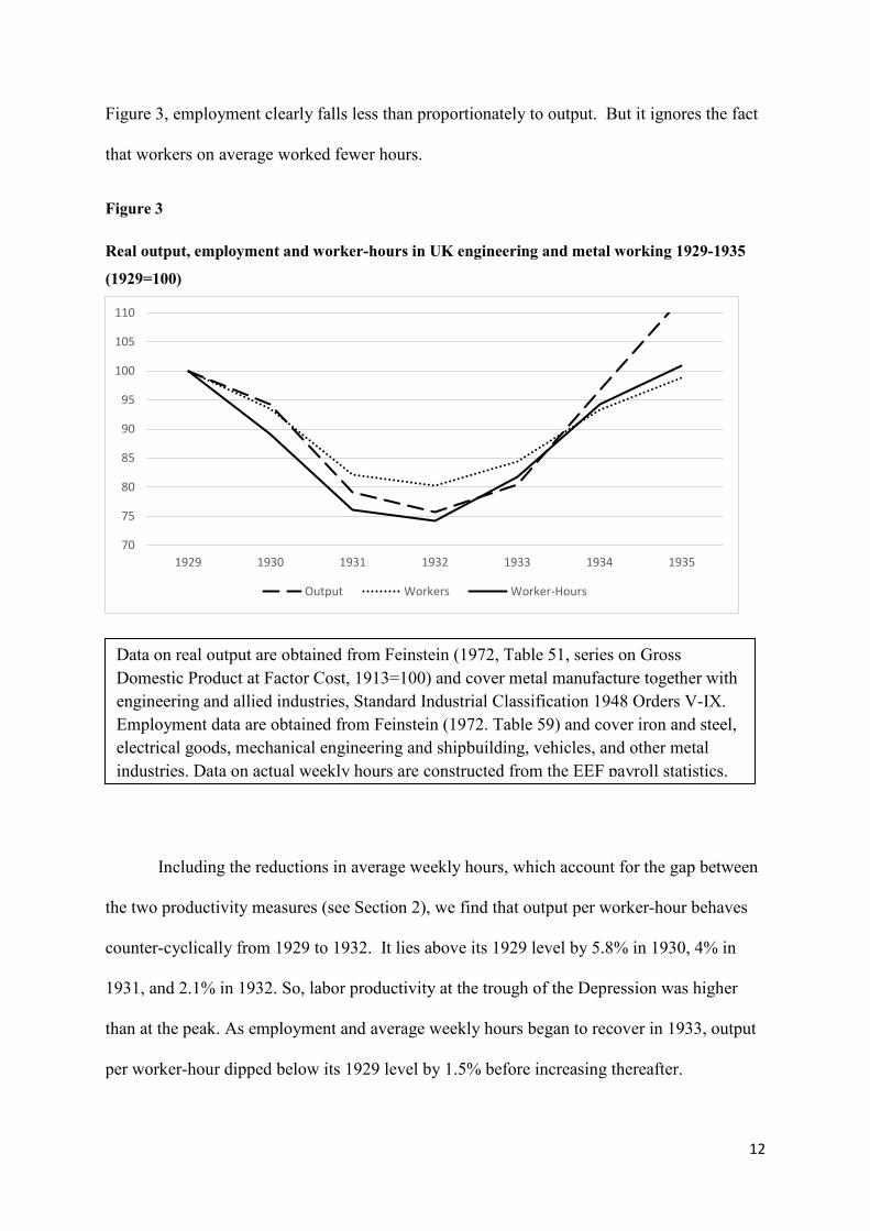
Figure 3 shows the movements of real output, employment and worker-hours from
1929 to 1935, with 1929=100. From 1929 to the 1932 trough, real output declined by 24%,
employment by 20%, and worker-hours by 26%. The relative steepness of the cutback in
worker-hours compared to employment in 1930 and 1931 reflects a comparatively speedier
adjustment of hours relative to jobs. 1932 marked a trough from which all three variables
started to rise. In the first recovery year, worker-hours rose more steeply than employment,
again indicative of speedier adjustment of hours relative to jobs. Thereafter there were strong
recoveries of both output and worker-hours. They regained their 1929 levels in 1935.
Figure 4 converts the information in Figure 3 to show the comparable movements of
output per worker and output per worker-hour (1929=100). After a slight rise of 0.9% in
1929-1930, output per worker is quite strongly procyclical, falling 5.6% between 1929 and
1932. Ignoring hours of work, this apparently indicates a classic labor hoarding story: from
8 These authors undertake their work on data from the interwar study of Bernanke and Parkinson (1991) that concentrates on wage earners.
12
Figure 3, employment clearly falls less than proportionately to output. But it ignores the fact
that workers on average worked fewer hours.
Figure 3
Real output, employment and worker-hours in UK engineering and metal working 1929-1935
(1929=100)
Figure 4
Including the reductions in average weekly hours, which account for the gap between
the two productivity measures (see Section 2), we find that output per worker-hour behaves
counter-cyclically from 1929 to 1932. It lies above its 1929 level by 5.8% in 1930, 4% in
1931, and 2.1% in 1932. So, labor productivity at the trough of the Depression was higher
than at the peak. As employment and average weekly hours began to recover in 1933, output
per worker-hour dipped below its 1929 level by 1.5% before increasing thereafter.
70
75
80
85
90
95
100
105
110
1929 1930 1931 1932 1933 1934 1935
Output Workers Worker-Hours
Data on real output are obtained from Feinstein (1972, Table 51, series on Gross Domestic Product at Factor Cost, 1913=100) and cover metal manufacture together with engineering and allied industries, Standard Industrial Classification 1948 Orders V-IX. Employment data are obtained from Feinstein (1972. Table 59) and cover iron and steel, electrical goods, mechanical engineering and shipbuilding, vehicles, and other metal industries. Data on actual weekly hours are constructed from the EEF payroll statistics.
13
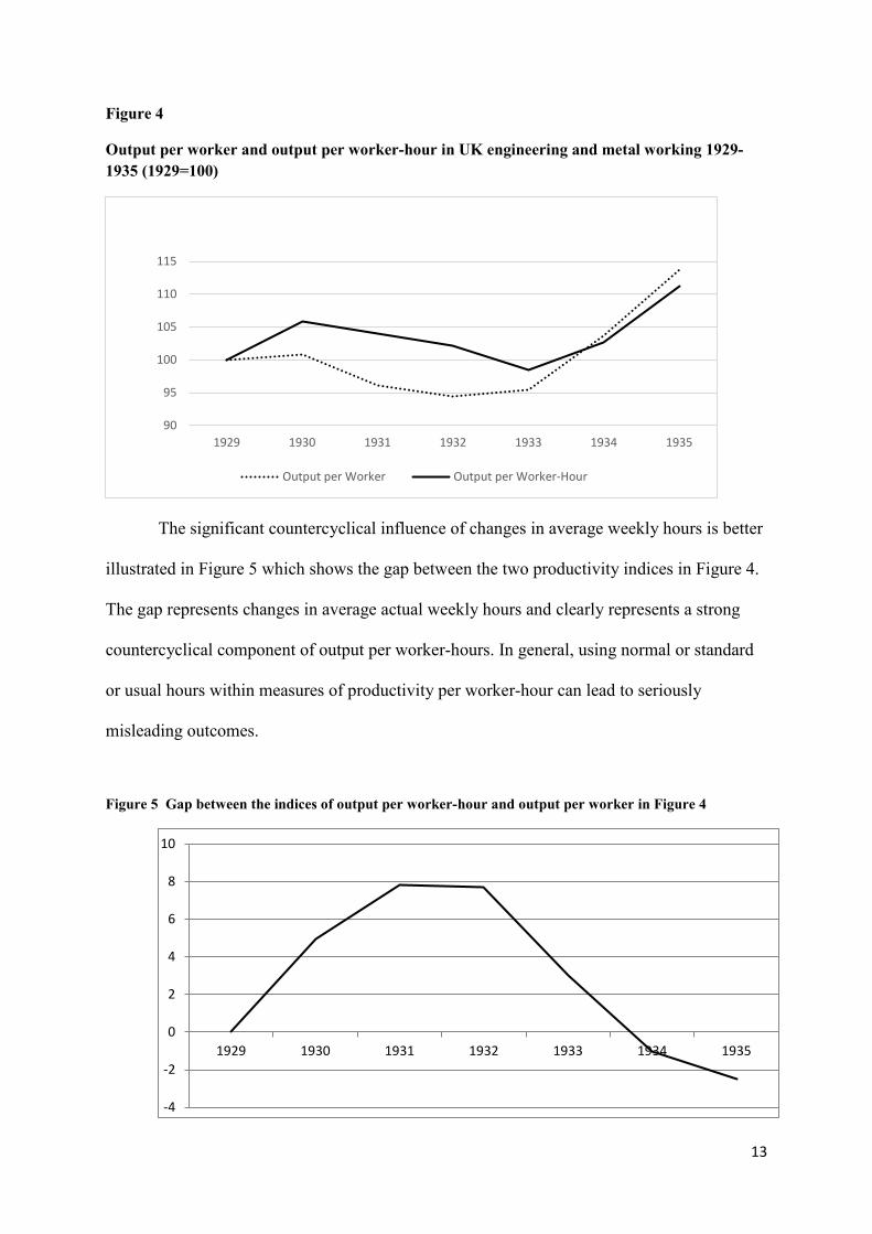
Figure 4
Output per worker and output per worker-hour in UK engineering and metal working 1929-1935 (1929=100)
The significant countercyclical influence of changes in average weekly hours is better
illustrated in Figure 5 which shows the gap between the two productivity indices in Figure 4.
The gap represents changes in average actual weekly hours and clearly represents a strong
countercyclical component of output per worker-hours. In general, using normal or standard
or usual hours within measures of productivity per worker-hour can lead to seriously
misleading outcomes.
Figure 5 Gap between the indices of output per worker-hour and output per worker in Figure 4
90
95
100
105
110
115
1929 1930 1931 1932 1933 1934 1935
Output per Worker Output per Worker-Hour
-4
-2
0
2
4
6
8
10
1929 1930 1931 1932 1933 1934 1935
14
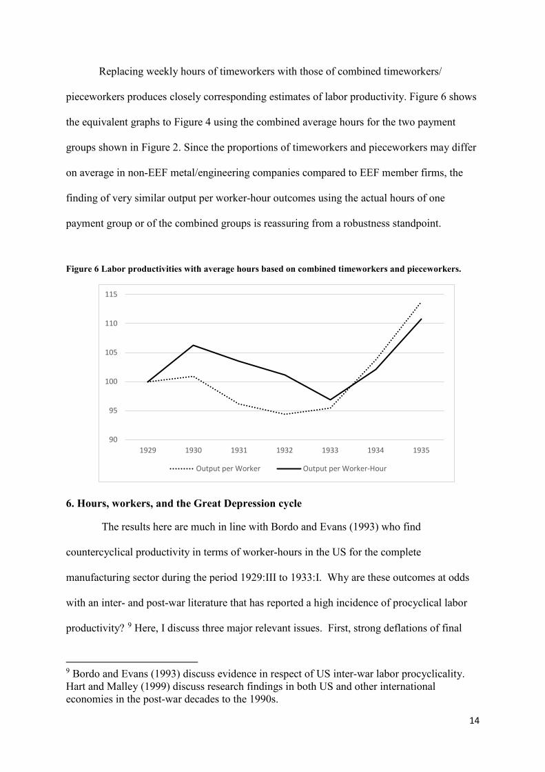
Replacing weekly hours of timeworkers with those of combined timeworkers/
pieceworkers produces closely corresponding estimates of labor productivity. Figure 6 shows
the equivalent graphs to Figure 4 using the combined average hours for the two payment
groups shown in Figure 2. Since the proportions of timeworkers and pieceworkers may differ
on average in non-EEF metal/engineering companies compared to EEF member firms, the
finding of very similar output per worker-hour outcomes using the actual hours of one
payment group or of the combined groups is reassuring from a robustness standpoint.
Figure 6 Labor productivities with average hours based on combined timeworkers and pieceworkers.
6. Hours, workers, and the Great Depression cycle
The results here are much in line with Bordo and Evans (1993) who find
countercyclical productivity in terms of worker-hours in the US for the complete
manufacturing sector during the period 1929:III to 1933:I. Why are these outcomes at odds
with an inter- and post-war literature that has reported a high incidence of procyclical labor
productivity? 9 Here, I discuss three major relevant issues. First, strong deflations of final
9 Bordo and Evans (1993) discuss evidence in respect of US inter-war labor procyclicality. Hart and Malley (1999) discuss research findings in both US and other international economies in the post-war decades to the 1990s.
90
95
100
105
110
115
1929 1930 1931 1932 1933 1934 1935
Output per Worker Output per Worker-Hour
15
output and consumer prices between 1929 and 1934 gave rise to an economic climate
conducive to significant hours’ reductions from both supply and demand perspectives.
Second, potential procyclical effects of labor hoarding were constrained by the sheer
magnitude of the peak-to-trough decline in production over a prolonged three-year period.
Third, long workweeks in interwar manufacturing were conducive to diminishing returns to
weekly hours.
(i) The demand and supply of hours
Starting in 1929 there was a period of severe price deflation in the UK. Between 1929 and
1934, final output prices fell by 13% while consumer goods and services prices fell by 11%
(Feldstein, 1972, Table 61).
On the demand side, falling product prices were associated with both employment and
working time reductions. In the case of working time, employers would have been motivated
by attempts to counter a fall in the marginal revenue product of hours by cuts in their
marginal cost. Given hourly earnings comprise a major element of marginal cost, an
especially important objective would have been to cut the high marginal costs associated with
overtime working.10 As illustrated in Figure 2, overtime was in important part of labor input
from 1927 to 1929. By 1931, overtime had been virtually eradicated in northern districts of
the UK. Given long weekly hours, increasing returns associated with cuts in working time
may have been realised over a range of hours covering overtime working and extending into
short-time working (see below). 10 Between 1920 and 1931, the overtime premium was paid at one and a half times the standard rate and at double the rate on Sundays. After 1931, the first 2 daily hours of overtime were paid at time and a third (Knowles and Hill, 1954 Appendix B). Both timeworkers and pieceworkers were eligible for overtime premium pay. Pieceworkers received their premium ‘mark-ups’ via a so-called minimum piecework standard (see Knowles and Hill, 1954).
16
The supply side of weekly hours in this period is more ambiguous. Average nominal
hourly wages of timeworkers during the Depression were flat while those of pieceworkers
were mildly procyclical (Hart and Roberts, 2013).11 The steep fall in consumer prices caused
real hourly earnings of both timeworkers and pieceworkers to rise significantly over the
depression years. Given high average weekly hours in the boom years of 1927 to 1929,
increasing real wages in 1928 and 1929 may well have produced income effects among many
workers leading to supply-side preferences to reduce weekly hours. As the Depression set in,
rising real hourly earnings would generally have served to softened resistance among workers
to employers desires to reduce weekly hours, especially when the threat of unemployment
was high.
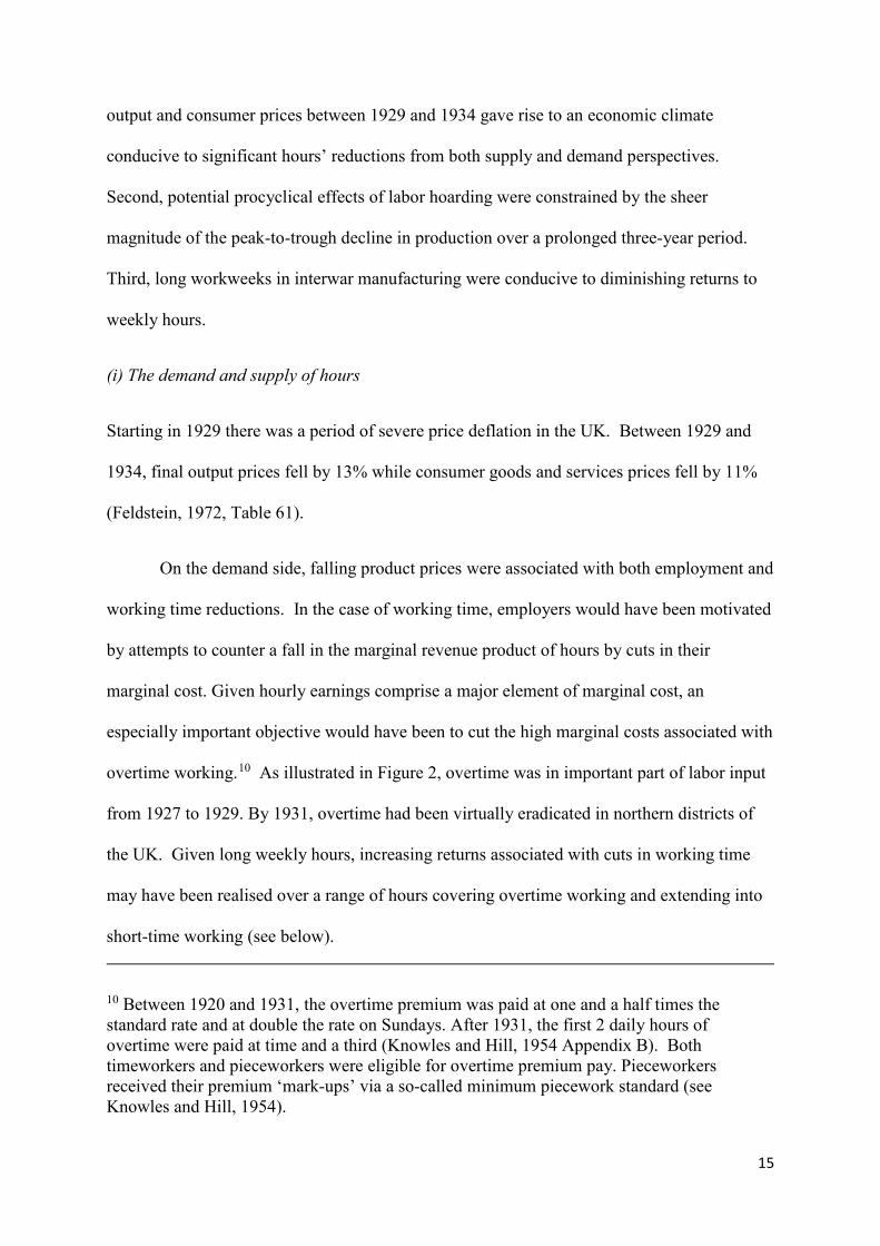
Figure 7a Real wages and real earnings of EEF timeworkers (1927-1937; 1927=100)
11 A downward movement of hourly earnings among piecework was due to an overt move in engineering to reduce the piecework-timework differentials. Earnings from piecework were linked to timework in the EEF. Up to mid-1931, piecework prices were generally set so that the average pieceworker earned at least one-third more than the equivalent time rate. After mid-1931 to 1943 this reduced to 25% (see Knowles and Hill (1954, p.281).
97
102
107
112
1927 1928 1929 1930 1931 1932 1933average hourly wage average hourly earnings
average weekly earnings
The hourly wage excludes overtime. Wages and earnings are deflated by the final output prices index (Feldstein, 1972, Table 61)
17
Table 7a shows the changes in real hourly wages, real hourly earnings, and weekly
real earnings of timeworkers in the EEF.12 Real hourly wages and earnings rose steeply
between 1928 and 1933. The lower rise in real hourly earnings relative to real hourly basic
wage rates reflects a fall in the share of premium overtime pay. In contrast, cuts in weekly
hours produced falls in real weekly earnings between 1929 and 1931. Note, however, over
the whole period of the Depression, real weekly earnings did not fall below their average
level of 1929 when the deflationary process started.
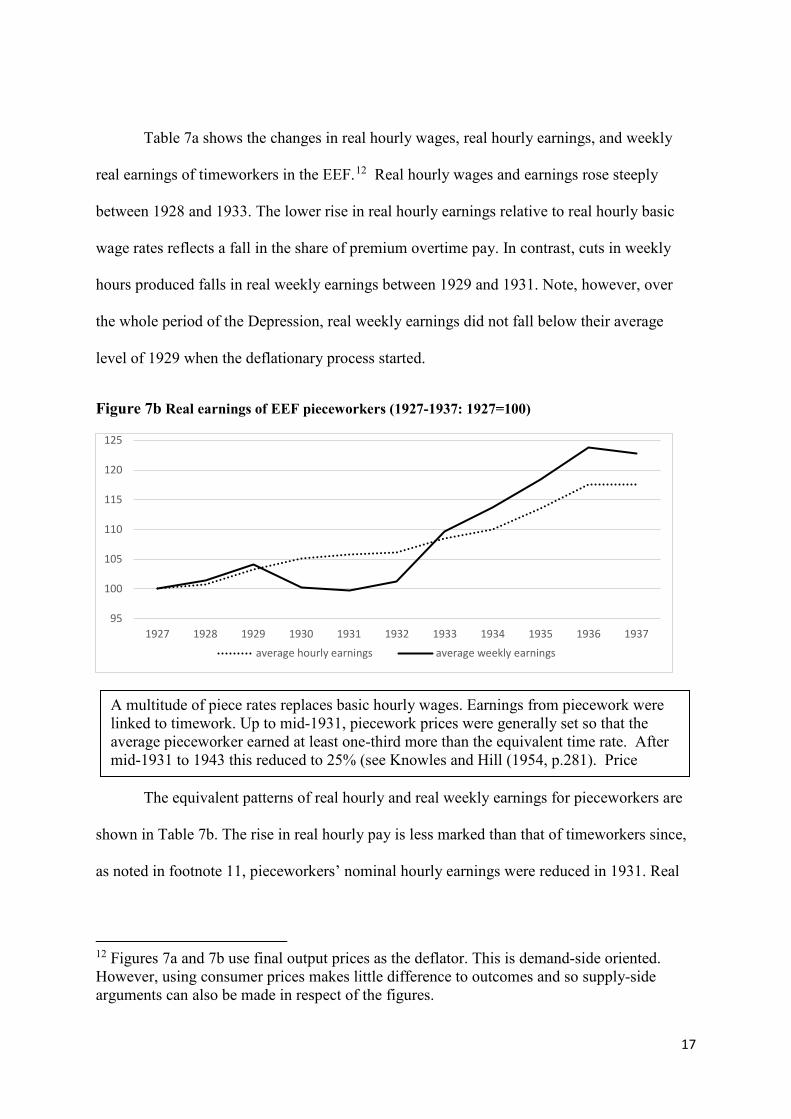
Figure 7b Real earnings of EEF pieceworkers (1927-1937: 1927=100)
The equivalent patterns of real hourly and real weekly earnings for pieceworkers are
shown in Table 7b. The rise in real hourly pay is less marked than that of timeworkers since,
as noted in footnote 11, pieceworkers’ nominal hourly earnings were reduced in 1931. Real
12 Figures 7a and 7b use final output prices as the deflator. This is demand-side oriented. However, using consumer prices makes little difference to outcomes and so supply-side arguments can also be made in respect of the figures.
95
100
105
110
115
120
125
1927 1928 1929 1930 1931 1932 1933 1934 1935 1936 1937
average hourly earnings average weekly earnings
A multitude of piece rates replaces basic hourly wages. Earnings from piecework were linked to timework. Up to mid-1931, piecework prices were generally set so that the average pieceworker earned at least one-third more than the equivalent time rate. After mid-1931 to 1943 this reduced to 25% (see Knowles and Hill (1954, p.281). Price
18
weekly pay fell by 4% between 1929 and 1930 and remained quite flat over the following
two years before staging a steep recovery in 1933.13
Final output price deflation helped to provide a strong stimulus for employers to
reduce both employment and weekly hours. The accompanying fall in consumer prices
served to temper supply-side resistance to shorter weekly hours.
(ii) Labor hoarding
A very common argument in studies that find support for procyclical labor
productivity features labor hoarding linked to labor’s quasi-fixity. An unanticipated negative
demand shock may lead to a drop in labor utilization as firms hold on to employees with
firm-specific skills and know-how, and who are generally reliable, productive, and well
matched to their job tasks. Short-term costs associated with underutilized labor resources are
traded-off against the expected longer term returns from future service flows from such
human assets. But labor hoarding is perhaps most suited to milder and shorter recessions
(Bordo and Evans, 1993). From its outset, the demand shock in late 1929 threatened seriously
to disrupt or put an end to future company business prospects. As stated by Bordo and Evans
for US manufacturing, “the length and severity of the Great Depression (1929-1933) suggests
that the costs of adjusting employment and honoring implicit long-term employment
contracts were second-order relative to the losses that many firms and industries
experienced”. Under these circumstances, a primary concern was to reduce the stock and
utilization of labour inputs while preserving productive performance. National averages do
not rule out pockets of labor hoarding but it is hard to imagine that these would have been
other than on a modest scale. 13 Based on the EEF data disaggregated by timework/piecework, occupations, and districts over the 1927-37 period, Hart and Roberts (2013) find that real hourly earnings were acyclical for timeworkers and mildly procyclical for pieceworkers. By contrast, real weekly earnings were strongly procyclical for both groups.
19
(iii) Diminishing returns to weekly hours
An absence of significant labor hoarding stops short of explaining countercyclical
labor productivity. We know from Figures 3 and 4 that if weekly hours had shown little
variation, then labor productivity would have been found to be procyclical. But actual hours
were highly variable and output per worker-hour turned out to be countercyclical. This at
least suggests that changes in hours of work over the Depression cycle played an important
role in explaining this outcome. A key question centres on the relationships in the production
function featuring changes in weekly output and weekly hours.14 A concave function would
indicate decreasing returns. For example, workers experiencing reductions in their fatigue
and stress levels when moving from 50-hour work weeks in 1927-1929 to 45 or fewer hours
in 1931 and 1932 may well have improved their hourly productive performances. An
alternative explanation for some workers over the same time interval is that an awareness of
rapidly growing layoffs and unemployment in their local engineering labor markets may have
encouraged improved work application and effort in order to reduce their own layoff
probabilities.15 Unfortunately, the EEF does not supply weekly output data and so such
effects cannot be directly tested.
Pencavel (2018) produces micro evidence of diminishing returns to weekly hours
based on British and US datasets. There are reasons for expecting that diminishing returns
14 It is perhaps reasonable to assume a more or less fixed capital stock over the early 1930s period. 15 Total male unemployment weighted across the first 29 districts shown in Figure 1 more than doubled between 1929 and 1932, from 11.7% to 25.3%. These districts account for 85% of the EEF workforce.

20
may especially occur within firms employing workers over very long weekly hours.16 In his
study of British munitions workers in WW1, diminishing returns are observed in respect of
weekly hours in excess of 44.17 To the extent that this finding might applied to the firms
included here18, especially in the traditional industries of the northern districts, at least we
know that many thousands of workers experienced working time reductions within the hours
interval consistent with Pencavel’s estimates supporting diminishing returns.
If diminishing returns to weekly hours played an important role in the observation of
improved output per worker-hour during the Depression, then why were long workweeks pre-
Depression a general labor market feature? Pencavel (2018) suggests that employers may not
have been aware of the possibility of enhanced returns to shorter hours. Extreme economic
circumstances forced many employers to cut working time in the early 1930s. The scale was
such that it is hard to imagine that they would have failed to observe increased productivity
per hour if diminishing returns to long hours had played an important role. Was a lesson
learned? The evidence is mixed. On the one hand, within a few years after the upturn in the
Depression cycle, long hours had been regained and remained very high up to and during
WW2. However this largely reflected the unusually intense pressure of demand for
16 Although diminishing returns can apply to relatively short-hourly schedules, especially where performance is closely monitored and work intensity is high. For example, using micro panel data for a call center in the Netherlands, Collewet and Sauermann (2017) find that a 1 percent increase in effective work time increases output by 0.9 percent in an environment where average effective daily hours are 4.6 hours. 17 This work is based on both an augmented Cobb-Douglas production function that allows the elasticity of output with respect to weekly hours to vary with hours (Pencavel, 2018, Figure 7) and on a standard Cobb-Douglas function subdivided into short-hours and long-hours regimes (Pencavel, 2018, Table 4.5). Hours above 44 are statistically consistent with diminishing returns while those between 43 and 33 hours are statistically consistent with the hypothesis that hours vary proportionately with output. See also Pencavel (2015). 18 Munitions production itself was undertaken in some EEF member firms, an activity that was to become especially important in the run-up to and during WW2.
21
engineering and metal working military-related hardware combined with a labor shortage due
to military call-up. On the other hand, the standard workweek in engineering and metal
working industries was reduced by 3 hours in 1946.
7. Conclusions
Job losses, reductions in hours, and unemployment increases among manufacturing
workers in the Great Depression were of a much higher order of magnitude than experienced
in the recent Great Recession. An extreme negative demand shock accompanied by sharp
reductions in product prices and rises in real hourly labor costs threatened the survival of
firms and served to rule out a significant recourse to labor hoarding. This reduced the
likelihood of procyclical labor productivity among manufacturing firms. Labor hoarding was
far less discouraged during Great Recession in the UK. Falling real wages were among
factors that helped to produce relatively milder employment reductions (Coulter, 2016).
In contrast to present times, long workweeks predominated during the inter-war
period in the manufacturing industries featured here. With the exception of modern industries
such as electrical engineering, aircraft manufacture, and vehicle manufacture, the great
majority of traditional manufacturing industries reduced working hours quite considerably.
This may well have been an important cause of the finding of countercyclical labor
productivity in the Great Depression. Increasing returns to shortened weekly hours combined
with considerable employment layoffs and a low propensity to hoard labor help account for
the absence of a labor productivity problem associated with Great Depression in contrast to
the long-term fall in labor productivity in the recent Great Recession.
22
References
Barnett, Alina, Sandra Batten, Adrian Chiu, Jeremy Franklin, and Maria Sebastiá-Barriel. 2014. The productivity puzzle. Bank of England Quarterly Bulletin Q2, 114-128.
Bernanke, Ben S. and Martin L. Parkinson. 1991. Procyclical labor productivity and competing theories of the business cycle: some evidence from interwar U.S. Journal of Political Economy 99, 439-459.
Bordo, Michael D. and Charles L. Evans. 1993. Labor productivity during the Great Depression. National Bureau of Economic Research, Cambridge, MA.
Central Statistical Office. 1948. Standard Industrial Classification. London: His Majesty’s Stationary Office.
Collewet, Marion and Jan Sauermann. 2017. Working hours and productivity. IZA Discussion Papers, No.10722
Coulter, Steve. 2016. The UK labor market and the ‘great recession’. In: Myant, M., S. Theodoropoulou, and A. Piasna (eds.). Unemployment, Internal Devaluation and Labour Market Deregulation in Europe: Brussels, Belgium, European Trade Union Institute, 197-227.
Feinstein, Charles, H. 1972. National Income, Expenditure and Output of the United Kingdom 1855-1965. Cambridge: Cambridge University Press.
Feldstein, Martin S. 1967. Specification of the labour input in the aggregate production function. Review of Economic Studies 34, 375-386.
Hart, Robert A. and Donald I. MacKay. 1975. Engineering earnings in Britain, 1914-1968. Journal of the Royal Statistical Society Series A 138, 32-50.
Hart, Robert A. and James R. Malley. 1999. Procyclical labor productivity: a closer look at a stylized fact. Economica 66, 533-550.
Hart, Robert A. and J. Elizabeth Roberts. 2013. Real wage cyclicality and the Great Depression: evidence from British engineering and metal working firms. Oxford Economic Papers 65, 197-218.
Knowles, K.G.J.C. and T.P. Hill. 1954. The structure of engineering earnings. Bulletin of the Oxford University Institute of Statistics, September/October, 272-328.
Ministry of Labour. 1928. Report of an enquiry into apprenticeship training. (Sections VI and VII). London: HMSO
Mitchell, B.R. 1988. British Historical Statistics. Cambridge: Cambridge University Press.
Pencavel, John. 2015. The productivity of working hours. Economic Journal 125, 2052-2076.
Pencavel, John. 2018. Diminishing returns at work. Oxford: Oxford University Press.
Wigham, E. 1973. The Power to Manage. A History of the Engineering Employers’ Federation. London: Macmillan.
Willey, F T. 1956. Plan for shipbuilding. London: Fabian Tract #299.