DISCUSSION PAPER SERIES

IZA DP No. 10779

Mark BorgschulteJacob Vogler

Run For Your Life?The Effect of Close Elections on theLife Expectancy of Politicians

MAY 2017

Any opinions expressed in this paper are those of the author(s) and not those of IZA. Research published in this series may include views on policy, but IZA takes no institutional policy positions. The IZA research network is committed to the IZA Guiding Principles of Research Integrity.The IZA Institute of Labor Economics is an independent economic research institute that conducts research in labor economics and offers evidence-based policy advice on labor market issues. Supported by the Deutsche Post Foundation, IZA runs the world’s largest network of economists, whose research aims to provide answers to the global labor market challenges of our time. Our key objective is to build bridges between academic research, policymakers and society.IZA Discussion Papers often represent preliminary work and are circulated to encourage discussion. Citation of such a paper should account for its provisional character. A revised version may be available directly from the author.

Schaumburg-Lippe-Straße 5–953113 Bonn, Germany

Phone: +49-228-3894-0Email: publications@iza.org www.iza.org

IZA – Institute of Labor Economics

DISCUSSION PAPER SERIES

IZA DP No. 10779

Run For Your Life?The Effect of Close Elections on theLife Expectancy of Politicians

MAY 2017

Mark BorgschulteUniversity of Illinois at Urbana-Champaign and IZA

Jacob VoglerUniversity of Illinois at Urbana-Champaign

ABSTRACT

MAY 2017IZA DP No. 10779

Run For Your Life?The Effect of Close Elections on theLife Expectancy of Politicians*

We use a regression discontinuity design to estimate the causal effect of election to political

office on natural lifespan. In contrast to previous findings of shortened lifespan among US

presidents and other heads of state, we find that US governors and other political office

holders live over one year longer than losers of close elections. The positive effects of

election appear in the mid-1800s, and grow notably larger when we restrict the sample to

later years. We also analyze heterogeneity in exposure to stress, the proposed mechanism

in the previous literature. We find no evidence of a role for stress in explaining differences

in life expectancy. Those who win by large margins have shorter life expectancy than either

close winners or losers, a fact which may explain previous findings.

JEL Classification: I10, M12, J14

Keywords: mortality, stress, regression discontinuity

Corresponding author:Mark BorgschulteDepartment of EconomicsUniversity of Illinois, Urbana-Champaign1407 W Gregory DriveUrbana, IL 61801USA

E-mail: markborg@illinois.edu

* We would like to thank Ernesto Dal Bo, Ronald Lee, Darren Lubotsky, Chris Tamborini and Rebecca Thornton, and seminar participants at University of Illinois at Urbana-Champaign and the Population Association of America Annual Meetings for comments and other assistance. Allen Gurdus, Carmen Ng, Megan Lindgren, Qinping Feng, Collin Schumock, Mya Khoury and Ben Moberly provided valuable re-search assistance.

Recent research finds that losing candidates in elections for head of state out-

live winners by large margins, suggesting a deleterious effect of political service

on longevity.1 The finding of harmful effects of service on life expectancy carries

immediate, but largely unexplored implications for both the selection of office-

holders and optimal incentives for politicians. In so far as these effects apply to

other individuals in similar executive leadership positions, such as CEOs, man-

agers of large organizations, and lesser political officeholders, they may explain

patterns in inequality and the compensation of superstars. And yet, despite the po-

tential wide-ranging significance of a loss of life expectancy from service as head

of state, the robustness, external validity, and mechanisms behind these estimates

remain unexplored. In particular, studies of US presidents and other heads of state

necessarily rely on small sample sizes, limiting more extensive analysis.

Aside from the implications for politicians and executives, findings in this area

engage with a long-standing medical and social science literature that hypothe-

sizes a role for stress arising from one’s relative position in social hierarchies in

creating health and lifespan differences.2 Theories of stress and life expectancy

associate decreased control over work tasks and surroundings with shorter life ex-

1US presidents die of natural causes around four years earlier than losing candidates (Linket al. 2013 and Borgschulte 2014); effects are somewhat smaller for a pooled sample of heads ofstate in Olenski et al. (2015). See also Olshansky (2011). The first comparison of winning andlosing presidential candidates we are aware of is Weyl (1973).

2Stress activates “fight or flight” physiological responses, which are understood to damagehealth with repeated exposure. For overviews of evidence on work-related stress and acceleratedaging, see McEwen (1998), Marmot (2004), Lupien et al. (2009), and Kivimaki et al. (2012).Work-related stress has been proposed as an explanation for countercyclical mortality (Ruhm2000, Ruhm 2005). Cutler et al. (2006) and Cutler et al. (2008) discuss stress-related theoriesof mortality and their relationship to economic factors.

2

pectancy. While exposure to this type of stress is usually thought to be negatively

correlated with rank in social hierarchies, a refinement of the theory suggests a U-

shaped exposure to stress, in which those at the top of a hierarchy may experience

a similar loss of health, particularly in response to instability in their position.3

A related literature in corporate finance points out that executives may use their

autonomy to live a “quiet life,” reducing their exposure to stress (Yen and Benham

1986, Bertrand and Mullainathan 2003). Despite the wide reach of these theories,

quasi-experimental evidence on the effects of prestige and stress is limited.4

In this paper, we estimate the causal effect of election to political office on

longevity, using a regression discontinuity (RD) model applied to a newly col-

lected dataset on winning and losing candidates for the offices of US governor

and senator, and representatives standing for re-election.5 A primary contribution

of the paper is the creation of a dataset that includes the dates of birth and death

and some biographical details on 100% of winning candidates and over 96% of

losing candidates in US history who fall within the appropriate RD bandwidth.6

The combined sample is over 100 times larger than that of presidents, with over

3Evidence on this theory largely comes from animal studies (Sapolsky, 2005).4Two quasi-experimental papers stand out: Anderson and Marmot (2012) finds a protective

effect of civil servant promotions induced by retirements, which they interpret as the effect ofrank; and Rablen and Oswald (2008) finds that Nobel prize winners outlive nominees, a protectiveeffect of prestige. Quasi-experimental evidence on the effects of stress specifically appears to bemore limited.

5We thank Ernesto Dal Bo for providing the representatives portion of the data. Data collectionfor candidates who never serve as representatives would be far more difficult than for governorsor senators.

6The rates we find candidates decline with the bandwidth, but we did find over 90% of can-didates within 20% of the margin of victory, and pass covariate and density tests at the threshold(McCrary, 2008).

3

50 times the sample within the RD bandwidth. The much larger sample size in our

dataset allow us to exclude candidates far from the margin of victory, greatly lim-

iting the scope for selection. In addition, we can use supplementary information

to test for heterogeneity in survival consistent with a role for stress.

Contrary to previous work on heads of state, we find that candidates who nar-

rowly win election experience an increase in natural life expectancy. The RD

model estimates that election is associated with 2.2 years of additional life, and

the result is significant at p < 0.01. When we add controls to the RD model,

suggested by Calonico et al. (2016) to improve efficiency, the effect falls to just

above a year of life gained. The effects are larger in both magnitude and signif-

icance after the mid-1800s.7 The RD design allows us to interpret our estimates

as the average causal effect of election to these offices for candidates who are

close to the margin of victory. The point estimates are similar across the three of-

fices, with larger and more significant effects for governors than representatives;

standard errors are too large to infer much about senators on their own.

Although our main estimates do not correspond with previous findings for

heads of state, we can use our larger sample size to test for heterogeneity con-

sistent with an effect of stress on life expectancy. It may be that the job of head

of state is considerably more stressful than the offices we study, however, if the

results from heads of state generalize to any group, we would expect to find some

evidence of differential survival among those who serve in the most stressful sit-

7Our primary cut to the later era is post-1908, as this was the year popular election of senatorsbegan. However, we also provide a non-parametric Lowess estimate of the difference betweenwinners and losers by year for our entire sample.

4

uations. We focus this analysis on US governors. As chief executives of their

state, governors are the most similar officeholders to US presidents; governors

are also the most likely individuals to win election as president.8 To proxy for

especially stressful periods of service, we identified a number of state character-

istics that would introduce challenges or uncertainty into the job.9 We also divide

candidates into different groups based on their likely vulnerability to stress.10 We

then fit interacted RD models that allowed differential effects of election in more

stressful situations.

We find no evidence that links stress experienced in office to the patterns of life

expectancy observed in the data. We take these results as suggestive, as most of

these characteristics reflect long-run trends in the states, and may induce selection

of more or less healthy individuals into candidacy. Despite this concern, it is

noteworthy that none of the characteristics we use to test for a role of stress shows

a significant negative effect on life expectancy. The evidence suggests that if there

is an important role for stress in explaining the lifespans of heads of state, the

effects are not experienced by similar executive officeholders, US governors. For

those who win close elections as governor, the effect of additional prestige and

income earned as a result of election appear to offset any loss of health due to

8An additional motivation for focusing on governors is practical — we could find biographicalinformation on a large number of both winning and losing candidates.

9The state characteristics we use in the main text are: the state population, total budget (rev-enues plus expenditures; we analyze these variables separately in the Appendix), a decrease in thestate population, and an indicator for divided government (i.e. the state legislature is controlled bya different party than the governor).

10The governor characteristics we use are indicators for being above age 50, first-time gover-nors, a change in party control in the governor’s office, no term limits, and the governor electedafter 1900.

5

service in office, even in the most stressful times.

We conclude with an analysis and discussion of reasons for the difference be-

tween our results and those for heads of state. Patterns in survival away from the

margin of victory call into question the assumption in previous work of an elec-

toral advantage for healthy candidates. Instead, we find that candidates who win

by a large margin have shorter life expectancy than those who win or lose close

elections. The negative relationship between vote share and survival is statistically

significant with and without controls, and is of similar magnitude to the (statisti-

cally insignificant) relationship between vote share and survival for US presidents.

This relationship could reflect selection and/or heterogeneity in the treatment ef-

fect. Selection would imply an electoral preference for less healthy candidates,

presumably due to a correlation with other desirable characteristics. Treatment

effect heterogeneity would imply that winning by large margins is worse for the

candidates’ health than a narrow victory; for example, this may occur if large-

margin victories predict longer careers, and career length is harmful. As the RD

model cannot inform us about these mechanisms, we leave detailed exploration of

these issue to future work.

1 Background and Data

1.1 Counterfactuals and Empirical Strategy

Our interest is in estimating the causal effect of winning a close election to po-

litical office on survival. The effect should be thought of as the combined conse-

6

quences of electoral victory, including not only the direct effects of service on the

health of the candidate (e.g. increased work and stress), but also the possibility

of future elections, promotion to higher political office, and increased prestige.

The election is treated as the randomization device, and survival is measured from

the date of the election. In the counterfactual, the candidate loses election, and

experiences the combined effects of this treatment.

Previous literature has relied on either life tables or losers to estimate the coun-

terfactual.11 The older literature compares the survival of presidents to statistical

life tables. This counterfactual likely understates the negative effects of service,

as elected officials are drawn from a wealthy, educated class of men with longer

life expectancy than the average. A more recent literature has attempted to esti-

mate the counterfactual through the comparison of winners and losers. This will

generate a lower bound on the negative effect of service under a “healthy winners”

assumption, wherein those with ex ante better health have an electoral advantage,

either through the direct preferences of the electorate or via their stamina during

the campaign.

In our analysis, we utilize a much larger sample of political candidates relative

to previous research to estimate a more compelling (and precise) counterfactual

by focusing on candidates who were close to victory or defeat.12 In our primary

11See Olshansky (2011) as a recent example of the life table method, and Link et al. (2013),Borgschulte (2014), Olenski et al. (2015), and Deuchert and Liebert (2016) as examples of thecomparison to losers. Deuchert and Liebert compares the survival of incumbent governors stand-ing for re-election in a regression discontinuity framework. See Appendix Section A for a longersummary and Appendix Table A1a and Appendix Table A1b for a list of papers dating back to1946.

12The RD design has been frequently employed to study close elections, as in Lee et al. (2004)

7

specification, we estimate a sharp regression discontinuity (RD) model for candi-

dates who have died before 2016. The model is:

Survivalit = β0 +β1Winnerit + f (Marginit)+g(Marginit)Winnerit + εit .

The outcome variable we consider is years of survival for candidate i following

election at date t. The running variable, Marginit , is defined as the difference in

vote share between what candidate i actually received and what was required to

win the election. Winnerit is our treatment variable, an indicator for winning the

election, and εit represents the error term. The main coefficient of interest is β1,

which we interpret as the causal impact of winning close political election on life

expectancy.

We implement local-linear regression for f and g, allowing for the slope of

the regression to be different on either side of the cutoff for victory. Robust, bias-

corrected standard errors are clustered at the state level to correct for likely corre-

lations across candidates and we use inference procedures developed by Calonico

et al. (2014) and Calonico et al. (2016). The sample included in our primary

analysis is composed of gubernatorial, senate, and congressional candidates, as

opposed to individuals, who receive a share of the vote within 20% of the mar-

gin of victory. In our primary specification, we pool candidates from all three

offices together and exclude candidates that died of accidents, assassinations, and

other violent causes.13. We assume these causes of death are random and likely

and Dal Bo et al. (2009).13We include candidates that committed suicide, as this cause of death may reflect stress brought

8

unrelated to theories of the stress-induced aging. We also present results from

specifications where we focus separately at candidates from each office type.

The RD framework uses a common Mean Square Error (MSE) optimal band-

width for candidates on either side of the cutoff for victory. A triangular kernel

weighting function is used to construct the point estimators. The results are robust

to alternative bandwidth selections and kernel choices.14 Following the literature,

our preferred specification estimates the model without including covariates, al-

though we also present estimates with controls that include quadratics in election

age and year, sex, state, political party, and both an indicator for previous service

in office and the total years served.15

To test for a role for stress on governors, we re-run our baseline RD model

with interactions between Winnerit and characteristics of the state that would re-

quire governors to exert more effort to govern, and candidate characteristics that

suggest greater susceptibility to stress. We set the bandwidth to be the same as the

baseline RD analysis using only the sample of governors, for reasons discussed

in the introduction. While the regression discontinuity model delivers unbiased

estimates (Lee and Lemieux (2010)), it comes at the cost of an increase in the

variance of the estimates relative to a model that utilizes all of the data in the

sample. Therefore, we compliment the RD results with estimates obtained from a

about from holding office14In particular, we experimented using Epanechnikov and uniform kernel functions, as well as

separate MSE-optimal bandwidth choices below and above the cutoff for victory.15Higher-order terms in age and year are not significant. The party variable takes 3 values, for

Democrat, Republican, and other party (such as Whig or Populist).

9

Tobit model specified as follows:

Survivalit = β0 +β1Winnerit +β2Zit +β3Winnerit ×Zit +XitB+ ε̃it .

Here, Zit represents a stressful state or candidate characteristic and we interpret

β3 as the causal effect of candidate i winning a close election and being exposed

to the stressful characteristic on survival. We treat candidates who are still alive

or died of violent and accidental causes as censored observations, and assume the

error follows the normal distribution, with the variance permitted to depend on the

age of the candidate at election. The sample includes all gubernatorial candidates

who receive a share of the vote within 20% of the margin of victory. In practice,

both the RD and Tobit models yield similar results when we test for the role of

stress.16

1.2 Data and Summary Statistics

Data on election results and the lives of US governors comes from Glashan (1979)

for candidates in elections from 1789-1960. Election data from later years is

taken from Congressional Quarterly. Election results for US senators and repre-

sentatives is gathered from ICPSR 3331: Database of Congressional Historical

Statistics. Senate election data includes the years 1908-1994 while data on repre-

sentatives is available from 1823-1994. The most challenging sourcing was data

on the birth and death dates (or whether the candidate is still living) of the losing

16A survival analysis yielded similar results to the RD and Tobit analysis.

10

gubernatorial and senate candidates. Biographical information for these candi-

dates comes from a variety of sources, including individual searches of historical

records. All biographical information were verified using as many sources as pos-

sible and checks to identify incorrect data entries were performed throughout the

data collection process.17 In sum, biographical information was found for 100%

of winning candidates and over 96% of losing candidates within the MSE-optimal

RD bandwidth.18

Summary statistics on age at election and age at death for candidates within the

optimal bandwidth of each sample are reported in Table 1. The table is restricted

to candidates that died of natural causes, and are nearly identical for the sample

including all candidates. In the pooled sample we find that winners and losers are

effectively balanced on age at election, with a statistically insignificant difference

of approximately .11 years between the groups. When looking specifically across

each office-type, we find a statistically insignificant difference in age at election

for both gubernatorial and congressional candidates. For senate candidates, the

average winner is 1.85 years older at election than the loser. This difference is

significant at the .05 level.

Turning to age at death, winning and losing candidates in the pooled sample

both survive about 23 years after the election, with the average age at death be-

17Online encyclopedias such as wikipedia.org proved useful starting points in the searches butwere not allowed to be used as the primary source. Any biographical information obtained fromsimilar resources were required to be verified using other sources. The Online Appendix providesmore information on the sources and construction of the dataset.

18Table C1 reports the percentages of candidates found within the pooled RD bandwidth. Ap-pendix Table C2 reports the percentages of found candidates within the 20% margin required forvictory, i.e. the total sample included in the RD analysis.

11

tween 73 and 74 years of age. There are no remarkable differences when examin-

ing average survival after election across office-types, however senate candidates

in the sample live about 5 to 6 years longer than gubernatorial and congressional

candidates. By comparison, US presidents stand for election, on average, at 56

years of age, and survive about 18 years when death is due to natural causes

(Borgschulte, 2014). The pooled sample size of 5711 candidates within the RD

bandwidth is also vastly larger than the total sample of 112 US presidential can-

didacies (counting only winners and runners-up) to date.

2 Survival of Political Candidates

We begin this section by discussing the estimated “first-stage” relationship be-

tween winning close political election and number of years served in office. When

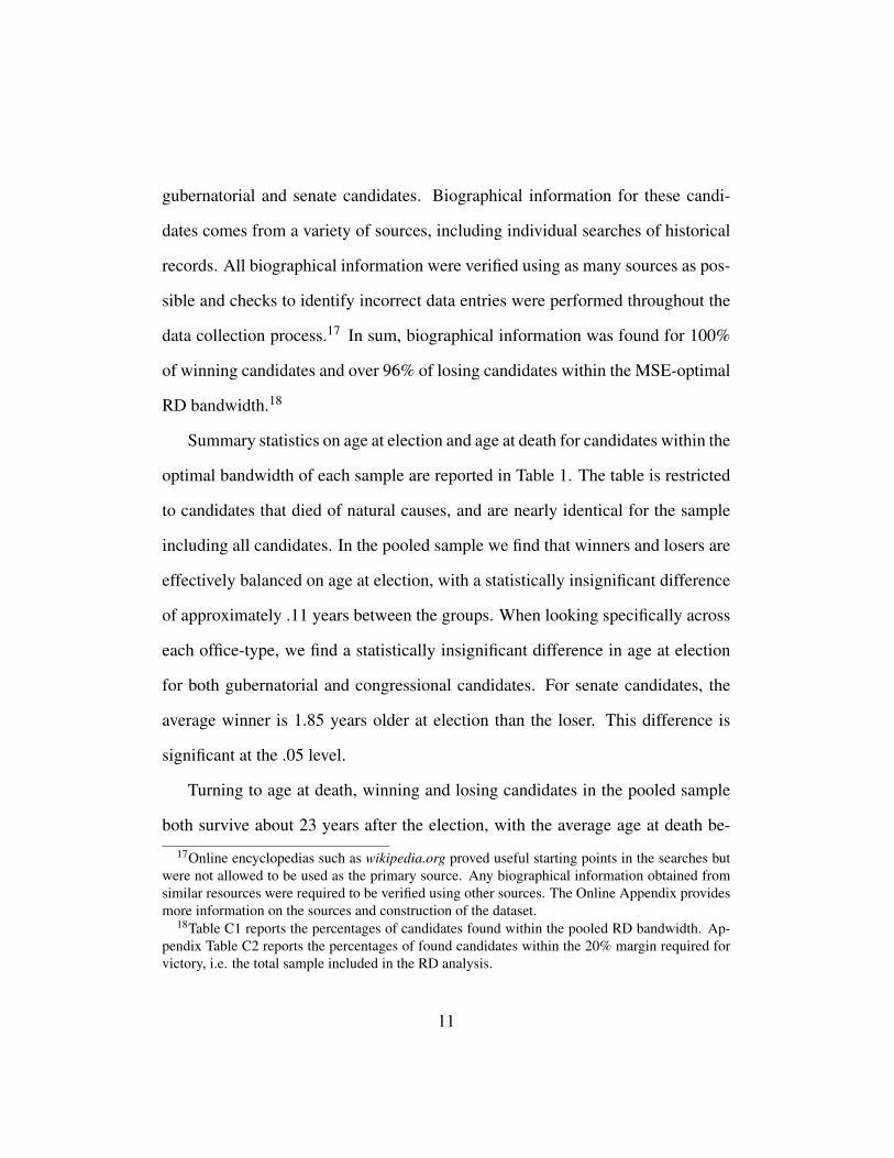
we pool candidates in our sample, Figure 1a shows winners of close political elec-

tions serve an average of 3.5 more years in office, with increasing slopes being

found on both sides of the cutoff for victory. This finding suggests a positive

relationship between number of votes received and total years of service. In Fig-

ure 1b, we find a similar upward sloping pattern on both sides of the cutoff when

we estimate the relationship between winning close political election and previous

years of service, though there is no detectable discontinuity.

Table 2 reports the results of the main RD longevity analysis for candidates

in the pooled sample. In Panel A we include all candidates that ran for office be-

tween 1789 and 2000. Column 1 presents baseline estimates without the inclusion

12

of covariates. We find winners in close elections live on average 2.22 years longer

than losers. This estimate is significant at the .01 level. The MSE-optimal band-

width includes candidates within 3.0% of the margin of victory, which is about

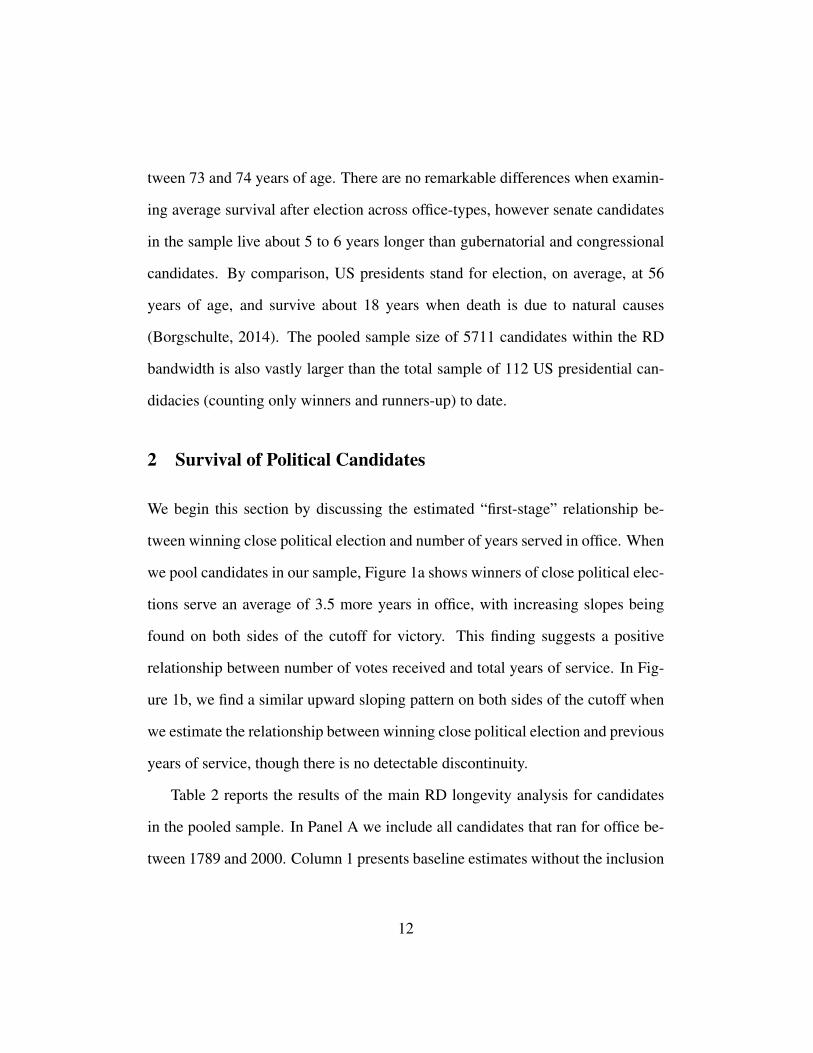
one-third of the nearly 21,000 candidates in our total pooled sample. Figure 2

depicts the estimated discontinuity in years of survival from Column 1. The local

linear functions show similar negative slopes on either side of the discontinuity,

and appear smooth.19

In Column 2 we add the full set of controls for age at election, year of election,

sex, party, state and previous service. The estimate of 1.18 years of longer life for

winners is smaller in magnitude than the baseline estimate, but remains significant

at the .05 level. The bandwidth also increases to include candidates within 3.5% of

the vote margin for victory. In Column 3, we remove controls and add candidates

who have died of violent or accidental causes, such as assassination or automo-

bile accidents. Excluding these individuals is especially important for analyses of

heads of state, as this is a unique risk faced by high-profile politicians, and unre-

lated to the broader question of the effects of executive service on health. Here,

only a small fraction of individuals have died of these causes, and the estimated

2.15 years of longer natural life for winners is very similar to results in Column

1. In Column 4, we include both controls and candidates that died of non-violent

and accidental causes. The estimated 1.08 of additional years of life for winners

19 Becker et al. (2008) find that retired players who narrowly miss election to the Major LeagueBaseball Hall of Fame have shorter survival than winners or those who do not approach the thresh-old for induction. We find no such “dip” in survival, once we account for the effect at the thresholdfor victory.

13

is marginally significant. In sum, we strongly reject the estimates in previous lit-

erature of significant loss of life due to service as head of state. Taken together,

our results suggest winners of close political races outlive losing candidates by

between 1 and 2 years after the election.20

When considering the implications of our findings for modern theories of life

expectancy, it may be more informative to focus on candidates who appear later

in our sample. In addition, our results in Panel A pool together our entire sample

of candidates, even though we have differing periods of coverage across the three

offices. With these concerns in mind, we re-estimate the model for candidates

that ran for election after 1908, the first year in which senators were popularly

elected and after which we have a nearly complete sample of all three offices. The

results appear in Panel B of Table 2. We find statistically significant estimates

that range between 2.0 and 3.4 years of longer life for winners in the post-1908

sample. The magnitude of the estimates in each specification are approximately

one year larger than the corresponding estimates in Panel A. Although it appears

the effect of winning a close election has increased over time, we cannot reject the

equality of the coefficients between the two panels.

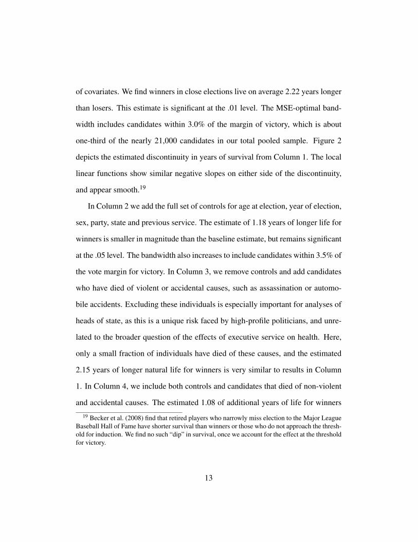
To better understand how survival between winning and losing candidates has

evolved over time, Figure 3 presents the average difference in survival between

winners and losers, by year of election, for candidates within the pooled sample

20By design, the RD specification does not differentiate between candidates that are still aliveand candidates that we were unable to find a date of death for. We might be concerned that the pointestimates are capturing some bias due to ignoring this difference. However, if election prolongslife, we would have slightly fewer candidates to the right of the cutoff. This would likely cause adownward bias on our point estimates.

14

MSE-optimal bandwidth. The non-parametric Lowess curve in the figure is fitted

to all of the data in sample, with 10-year binned markers scaled by the number of

observations within each bin. There are two important points to make here. First,

the figure shows losing candidates that ran prior to 1850 had longer average life

expectancies relative to winning candidates. However, for elections after 1850,

the average life expectancy for winners was consistently longer by approximately

one year. (Note that we do not include the RD polynomials here.) Second, the size

of the markers indicates that a large proportion of candidates in the sample died

after 1908, when candidates from each office type appear together. This further

motivates our restricting the sample in Panel B of Table 2.21

Considering the majority of candidates in our sample are representatives, we

might also be concerned that the main RD results are somehow biased as a result

of over-saturation of congressional candidates. We check the robustness of the

findings in Table 2 by restricting the sample to only gubernatorial and senate can-

didates. Across all specifications, we again find statistically significant evidence

that winning candidates outlive losing candidates by between 1.5 and 2.5 years

after the election.22

In Table 3, we extend the RD analysis by focusing separately on specific office

types. Columns 1 to 3 report results for gubernatorial candidates.23 In Column 1

the estimate suggests winning candidates live 1.15 years longer than losing candi-

21Figures C4, C5 and C5 depict the average difference in survival between winners and losersseparately by office-type.

22Results are presented in Appendix Table C3.23RD figures by office type appear in the Online Appendix.

15

dates, though the estimate is insignificant. When we include controls in Column 2

the estimated effect of winning increases to 1.63 years and becomes significant at

the .10 level. Including the few candidates that died of violent or accidental causes

in Column 3 does little to change the estimates. Overall, we find no evidence of

shorter lifespans for governors. Rather, the direction and magnitude of the point

estimates are in-line with our estimates using the pooled sample presented in Ta-

ble 2.

Columns 4 to 6 of Table 3 report results for candidates running for the office

of U.S. senator. In Column 4 the estimate suggests winners live 1.42 years longer

than losing candidates. This estimate is measured very imprecisely, with the stan-

dard error much larger than the point estimate. This is not necessarily surprising

considering the overall sample size used to construct the RD is only 1784 candi-

dates, of which only 687 observations lie within the MSE-optimal bandwidth. The

point estimate increases to 1.37 years of longer life for winners when we include

controls in Column 5 but remains insignificant. Including candidates that died of

violent or accidental causes reduces the size of the point estimate, although the

small sample size does not allow us to draw strong conclusions. In any case the

estimate is measured imprecisely with a standard error that is similar in magnitude

to Columns 4 and 5.

We present results for congressional representatives who stand for re-election

in Columns 7 and 8. The baseline estimate in Column 7 suggests winners outlive

losing incumbents by 1.86 years after the election. This estimate is marginally

significant. When we add controls to regression in Column 8, the point estimate

16

drops to three-quarters of an additional year of natural life for winners, and is no

longer statistically significant. Overall, we again find no evidence when examin-

ing representatives that winning close election to office decreases life expectancy

relative to losers. Rather, our estimates provide support for the opposite conclu-

sion, that winning a close election increases life expectancy.

2.1 RD Validity Tests

The validity of the estimates obtained using the RD design rest on the key assump-

tion that assignment to treatment near the cutoff for victory is essentially random.

If this assumption is true, then we can be confident that candidates who barely

lost an election are appropriate counterfactuals to candidates that barely won. A

potential threat to this assumption is if the construction of our sample generates

differences at the margin of victory threshold, in particular as winning candidates

are more likely to appear in the final dataset than losers. Another potential threat

to identification is if candidates can manipulate their treatment status. One exam-

ple of this would be if incumbent candidates in close elections have a systematic

advantage over their opponent.24 Importantly, both data construction and incum-

bency advantages would suggest excess mass to the right of the threshold.

With these potential threats in mind, we first test for evidence of violations of

the identifying assumption using the nonparametric test developed by McCrary

24Previous work has found evidence of manipulation in 20th century elections for representa-tives due to an apparent incumbency advantage. However, recent work by Eggers et al. (2015)suggests the potential for candidates to manipulate outcomes in close U.S. elections does not posea threat to the validity of RD designs in other electoral settings.

17

(2008). The general idea of the test in the context of our study is to examine the

density of observations near the cutoff for victory. If there is a discontinuity in

the density, then this may open the door to systematic differences between narrow

winners and losers, and biased estimates.25 Looking across all samples, we find

no evidence of discontinuities in the density. This greatly limits any potential

biases due to the construction of the data or the manipulation of close elections.

We further explore the validity of our RD design by testing whether the co-

variates included in relevant specifications are smooth through the cutoff. This

exercise is done for two main reasons. First, considering the RD design assumes

candidates that barely won are the same as candidates that barely lost, intuition

suggests that the candidates should not significantly differ based on observable

characteristics. Any discontinuity in survival that occurs as a result of assignment

to treatment, i.e. winning a close election, should not be explained by a disconti-

nuity in other observable characteristics. Second, if the observable covariates are

smooth throughout the cutoff, then inclusion of the these variables in the regres-

sion can be justified as simply increasing the precision of our estimates.

With this in mind, we conducted an additional RD analysis where the outcome

variable include pre-election measures, such as age at election, year of election,

gender, the number of previous years served, and and indicator for previous ser-

vice.26 Among all the estimates, we find only one marginally significant differ-

ence between winners and losers near the cutoff, for age at election in the pooled

25Appendix Table C4 provides results from the density test.26See Appendix Table C5.

18

sample. This is consistent with the reduction in magnitude of around 1 year when

we add controls to the regressions; age is naturally quite predictive of remaining

life expectancy. However, we argue this finding to be relatively inconsequential to

our main results considering the difference is only marginally significant and the

point estimate in the pooled RD analysis is robust to including age at election as

a control. We do not find evidence of significant differences in incumbency, the

most problematic variable identified by the previous literature. Overall, results

from the covariate test suggest discontinuities in observable characteristics do not

pose a major concern.

2.2 Heterogeneity by State and Governor Characteristics

The comparison of winning and losing candidates may differ from the effects for

presidents because of statistical issues in previous comparisons, or because the

jobs of these politicians are fundamentally different than that of heads of state.

The previous literature has pointed to an important role of stress in explaining

the apparently shortened lifespans of heads of state. We test for that channel by

examining heterogeneity in survival among governors based on the characteristics

of states and candidates.

To carryout this test, data was collected on a wide range of state and candidate

characteristics likely to be associated with higher levels of stress. For states, we

look at: state population with the idea being that larger states more closely resem-

ble the countries that are governed by heads of state and are therefore more stress-

ful to govern; size of the state government; percent change in the state population,

19

since decreasing populations likely signal a decline in state fortunes, therefore

being more stressful to govern; and an indicator for there being a divided gov-

ernment, i.e. when the state legislature is controlled by a different party than the

governor. For candidates, we examined: those above the age of 50 at election (the

mean election age) with stress predicted to be more harmful to older candidates;

those elected after 1900 as it is likely that serving in this period more closely re-

sembles the jobs performed by heads of state; those elected to their first term of

service; those elected from a different party than the previous governor; and those

elected that are not restricted to run again for re-election due to term limits.27

Panel A in Table 4 reports results for heterogeneity by stressful state charac-

teristics using the RD and Tobit models described in section 1.1.28 Columns 1 and

2 present results from the RD and Tobit specifications, respectively. Overall, we

find no evidence of shorter life expectancy for candidates elected to more stressful

positions. In the first two rows, we find larger states and larger government size

appear to increase the life expectancy of winners. The point estimates are similar

across both the RD and Tobit specifications. Larger states presumably present the

most comparable challenges to those faced by presidents and other heads of state,

so it is noteworthy that the estimated effect is of the opposite patterns as suggested

by the previous literature. In fact, this evidence is more consistent with a positive

prestige effect uncovered by previous researchers, than with an negative stress

effect (Rablen and Oswald 2008, Liu et al. 2015). The size of the state popula-

27See Appendix B for a detailed discussion of the data sources and construction of these vari-ables.

28Appendix Tables C6, C7 and C8 report the full results of the stress analysis.

20

tion and state budget are highly correlated, motivating us to examine a regression

including both terms. Results in the third row reveal that we cannot distinguish

whether population or size of government explains the larger-government effect.

In the fourth row, we find states with shrinking populations have governors who

live longer while estimates in last row of Panel A suggests governors who expe-

rience divided governments survive fewer years; none of these results are statisti-

cally significant. None of these results support the hypothesis that stressful states

harm their governors.

A similar pattern appears in Panel B of Table 4. In row 1 candidates elected

above the age of 50 show no evidence of shorter survival. In rows 2 and 3, the

point estimates for candidates serving in their first term and those elected from a

new party show the opposite pattern than hypothesized. In row 4, we find can-

didates that are not restricted from running again due to term limits live slightly

less, though both the RD and Tobit estimates are far from significant. Estimates

in row 5 shows candidates elected in the years after 1900 demonstrate superior

survival to winners in earlier periods, despite the growing populations and chal-

lenges across history. Consistent with the post-1908 analysis for all candidates,

estimates from the RD and Tobit specification range from 1.75 to 2.20 years of

longer life for winners elected after 1900. In sum, we find no evidence of shorter

lifespans among those who we theorize should be most vulnerable to the stresses

of holding office.

21

2.3 Revisiting the Evidence from US Presidential Candidates

We next turn to the question of why previous studies have found a shorter life

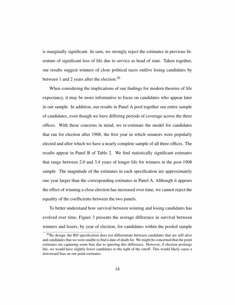
expectancy for presidents and other heads of state. In Figure 4 we plot the rela-

tionship between vote margin and survival for both US governors and presidents,

controlling for for age at election, year of election, and previous service. Both

presidents and governors exhibit a strong, negative relationship between the share

of the vote they receive and their subsequent survival. The slopes are nearly iden-

tical: an increase in vote margin by 10% is associated with 0.62 years reduced life

expectancy for presidential candidates, and 0.64 years reduced life expectancy for

gubernatorial candidates. The local linear RD terms are also negative for senators

and representatives. It appears the previous literature comparing election winners

to losers may have reached conclusions of a negative effect of service due to the

pooling of candidates near the margin of victory, who have similar survival to

those who narrowly lose, with candidates who win by large margins, who have

shorter survival.

As it is unlikely that the electorate prefers shorter-lived candidates, a natural

hypothesis is that candidates who win by large margins possess other character-

istics which make them especially electable, but are correlated with shorter lifes-

pans. Indeed, as Figure 1a and Figure 1b illustrate, not only do winners of close

political elections serve more years in office, but the increasing slopes on both

sides of the cutoff for victory suggest that candidates that win by large margins

tend to serve even longer.

We further investigated the possible sources of this negative selection on life

22

expectancy using the full set of covariates in our governors dataset, including

controls for state and party. The relationship between survival and vote margin

weakened to a slope of -0.50. We also found the change in slope was statisti-

cally significant for a number of covariates, including years of previous service

(estimate = -0.034) and age at election (estimate = -0.086). It appears age and

experience at least partially explain the issue of selection for governors, which is

not unexpected as many voters may prefer candidates that are older and more ex-

perienced to younger and inexperienced candidates. Still, we cannot fully account

for the life expectancy gradient in margin of victory. We surmise that there are

likely a host of other observable and unobservable characteristics that explain the

issue of selection on life expectancy.

3 Conclusion

Previous research finds that presidents and other heads of state suffer a loss of

health from their service, and assigns blame to the stress associated with the un-

certainty created by high-stakes decision-making and shifting political support.

This result has wide-ranging implications, should these effects be experienced by

other executives. We use the much larger sample sizes in our dataset of US guber-

natorial, senate, and congressional candidates to test whether these effects extend

to other, seemingly similar individuals. In contrast with the estimates of 4 years or

more of lost life found for presidents and other heads of state, we find that winning

close elections significantly increases life expectancy. As well, our larger dataset

23

allows for explicit tests for a role for stress among US governors, for which we

find no evidence along any of the dimensions we test. We conclude that the results

for presidents do not extend to other, similar individuals, and may reflect selection

rather than a causal effect of service.

We have focused our investigation of mechanisms on the role of stress in ex-

plaining life expectancy differences, as this channel may affect a wide range of

other individuals, and is relatively unexplored in the literature. However, alterna-

tive mechanisms may be at work. One possibility is that losing exerts a negative

effect on survival, if narrow losers experience profound disappointment or anxiety

from the experience. It is also possible that health losses to winning candidates

are offset by increases in prestige or income associated with service. While both

negative effects of losing and positive effects of increased prestige would pre-

sumably also be experienced by heads of state examined in previous studies, it is

nevertheless independently interesting to examine the evidence for among win-

ning political candidates. On the effects of losing, we find no “dip” in survival

for losing candidates near the discontinuity, but concede that losing may play an

important role in explaining our results. On the other hand, governors elected in

larger states and later in US history show signs of longer lives. These governors

presumably face increased job duties, but also may have more important roles in

the lives of their constituents and appointees. Taken together, our findings suggest

that prestige and other benefits of promotion to high offices more than offset any

health costs, even in the most stressful times.

24

References

Anderson, Michael and Michael Marmot (2012) “The Effects of Promotions on

Heart Disease: Evidence from Whitehall,” The Economic Journal, Vol. 121,

pp. 1–35, URL: http://dx.doi.org/10.1111/j.1468-0297.2011.02472.

x, DOI: http://dx.doi.org/10.1111/j.1468-0297.2011.02472.x.

Becker, David J., Kenneth Y. Chay, and Shailender Swaminathan (2008) “Mortal-

ity and the Baseball Hall of Fame: An Investigation into the Role of Status in

Life Expectancy,” Working Paper.

Bertrand, Marianne and Sendhil Mullainathan (2003) “Enjoying the Quiet Life?

Corporate Governance and Managerial Preferences,” Journal of Political Econ-

omy, Vol. 111, pp. 1043–1075.

Borgschulte, Mark (2014) “The Effect of Presidential Service on Life Ex-

pectancy,” First draft January 2012.

Calonico, Sebastian, Matias D Cattaneo, Max H Farrell, and Rocıo Titiunik (2016)

“Regression discontinuity designs using covariates,”Technical report, working

paper, University of Michigan.

Calonico, Sebastian, Matias D Cattaneo, and Rocio Titiunik (2014) “Robust

Nonparametric Confidence Intervals for Regression-Discontinuity Designs,”

Econometrica, Vol. 82, pp. 2295–2326.

Cutler, David, Angus Deaton, and Adriana Lleras-Muney (2006) “The Determi-

25

nants of Mortality,” Journal of Economic Perspectives, Vol. 20, pp. 97–120,

URL: http://www.aeaweb.org/articles.php?doi=10.1257/jep.20.3.

97, DOI: http://dx.doi.org/10.1257/jep.20.3.97.

Cutler, David M., Adriana Lleras-Muney, and Tom Vogl (2008) “Socioeconomic

Status and Health: Dimensions and Mechanisms,” Working Paper 14333, Na-

tional Bureau of Economic Research.

Dal Bo, Ernesto, Pedro Dal Bo, and Jason Snyder (2009) “Political Dynas-

ties,” The Review of Economic Studies, Vol. 76, pp. 115–142, URL: http://

restud.oxfordjournals.org/content/76/1/115.abstract, DOI: http:

//dx.doi.org/10.1111/j.1467-937X.2008.00519.x.

Deuchert, Eva and Helge Liebert (2016) “Aging faster in office? The Effect of

Extended Service in Political Office on Longevity,” Applied Economics Letters,

Vol. 23, pp. 510–515, DOI: http://dx.doi.org/10.1080/13504851.2015.

1083936.

Dubin, Michael J. (2010) United States Gubernatorial Elections, 1861-1911, The

Official Results by State and County: McFarland and Company.

(2013) United States Gubernatorial Elections, 1912-1931, The Official

Results by State and County: McFarland and Company.

Eggers, Andrew C, Anthony Fowler, Jens Hainmueller, Andrew B Hall, and

James M Snyder (2015) “On the validity of the regression discontinuity design

26

for estimating electoral effects: New evidence from over 40,000 close races,”

American Journal of Political Science, Vol. 59, pp. 259–274.

Glashan, Roy R. (1979) American Governors and Gubernatorial Elections, 1775-

1978: Mecklermedia Corporation.

Kivimaki, Mika, Solja T Nyberg, G David Batty, Eleonor I Fransson, Katri-

ina Heikkila, Lars Alfredsson, Jakob B Bjorner, Marianne Borritz, Hermann

Burr, Annalisa Casini, Els Clays, Dirk De Bacquer, Nico Dragano, Jane E Fer-

rie, Goedele A Geuskens, Marcel Goldberg, Mark Hamer, Wendela E Hooft-

man, Irene L Houtman, Matti Joensuu, Markus Jokela, France Kittel, Anders

Knutsson, Markku Koskenvuo, Aki Koskinen, Anne Kouvonen, Meena Ku-

mari, Ida EH Madsen, Michael G Marmot, Martin L Nielsen, Maria Nordin,

Tuula Oksanen, Jaana Pentti, Reiner Rugulies, Paula Salo, Johannes Siegrist,

Archana Singh-Manoux, Sakari B Suominen, Ari Vaananen, Jussi Vahtera,

Marianna Virtanen, Peter JM Westerholm, Hugo Westerlund, Marie Zins, An-

drew Steptoe, and Tores Theorell (2012) “Job strain as a risk factor for coronary

heart disease: a collaborative meta-analysis of individual participant data,” The

Lancet, Vol. 380, pp. 1491 – 1497, URL: http://www.sciencedirect.com/

science/article/pii/S0140673612609945, DOI: http://dx.doi.org/

http://dx.doi.org/10.1016/S0140-6736(12)60994-5.

Lee, David S. and Thomas Lemieux (2010) “Regression Discontinuity Designs in

Economics,” Journal of Economic Literature, Vol. 48, pp. 281–355.

Lee, David S., Enrico Moretti, and Matthew J. Butler (2004) “Do Voters Affect

27

or Elect Policies? Evidence from the U. S. House,” The Quarterly Journal of

Economics, Vol. 119, pp. 807–859.

Link, Bruce G., Richard M. Carpiano, and Margaret M. Weden (2013) “Can

Honorific Awards Give Us Clues about the Connection between Socioeco-

nomic Status and Mortality?” American Sociological Review, Vol. 78, pp. 192–

212, URL: http://asr.sagepub.com/content/78/2/192.abstract, DOI:

http://dx.doi.org/10.1177/0003122413477419.

Liu, Gordon G, Ohyun Kwon, Xindong Xue, and Belton M Fleisher (2015) “How

Much Does Social Status Matter to Longevity? Evidence from China’s Aca-

demician Election,” Health Economics.

Lupien, Sonia J, Bruce S McEwen, Megan R Gunnar, and Christine Heim (2009)

“Effects of stress throughout the lifespan on the brain, behaviour and cogni-

tion,” Nature Reviews Neuroscience, Vol. 10, pp. 434–445.

Marmot, Michael (2004) The Status Syndrome: How Social Standing Affects Our

Health and Longevity, New York: Holt.

McCrary, Justin (2008) “Manipulation of the running variable in the regression

discontinuity design: A density test,” Journal of Econometrics, Vol. 142, pp.

698–714.

McEwen, Bruce S. (1998) “Protective and Damaging Effects of Stress Media-

tors,” New England Journal of Medicine, Vol. 338, pp. 171–179, URL: http:

28

//www.nejm.org/doi/full/10.1056/NEJM199801153380307, DOI: http:

//dx.doi.org/10.1056/NEJM199801153380307.

Olenski, Andrew R, Matthew V Abola, and Anupam B Jena (2015) “Do Heads

of Government Age More Quickly? Observational Study Comparing Mor-

tality Between Elected Leaders and Runners-up in National Elections of 17

Countries,” British Medical Journal, Vol. 351, URL: http://www.bmj.com/

content/351/bmj.h6424, DOI: http://dx.doi.org/10.1136/bmj.h6424.

Olshansky, S. Jay (2011) “Aging of US Presidents,” JAMA: The Journal of

the American Medical Association, Vol. 306, pp. 2328–2329, URL: http://

jama.ama-assn.org/content/306/21/2328.2.short, DOI: http://dx.

doi.org/10.1001/jama.2011.1786.

Rablen, Matthew D. and Andrew J. Oswald (2008) “Mortality and Im-

mortality: The Nobel Prize as an Experiment into the Effect of Sta-

tus upon Longevity,” Journal of Health Economics, Vol. 27, pp. 1462

– 1471, URL: http://www.sciencedirect.com/science/article/pii/

S0167629608000775, DOI: http://dx.doi.org/10.1016/j.jhealeco.

2008.06.001.

Ruhm, Christopher J. (2000) “Are Recessions Good for Your Health?” The

Quarterly Journal of Economics, Vol. 115, pp. 617–650, URL: http://

qje.oxfordjournals.org/content/115/2/617.abstract, DOI: http://

dx.doi.org/10.1162/003355300554872.

29

Ruhm, Christopher J (2005) “Healthy Living in Hard Times,” Journal of Health

Economics, Vol. 24, pp. 341–363.

Sapolsky, Robert M. (2005) “The Influence of Social Hierarchy on Primate

Health,” Science, Vol. 308, pp. 648–652, URL: http://www.sciencemag.

org/content/308/5722/648.abstract, DOI: http://dx.doi.org/10.

1126/science.1106477.

Shavelle, Robert M, Scott J Kush, David R Paculdo, David J Strauss, and

Steven M Day (2008) “Underwriting the Presidents,” Journal of Insurance

Medicine, Vol. 40, pp. 120–123.

Weyl, Nathaniel (1973) “Letter to the Editor: Life Expectancy of Modern US

Presidents,” Perspectives in Biology and Medicine.

Yen, Gili and Lee Benham (1986) “The Best of All Monopoly Profits is a Quiet

Life,” Journal of Health Economics, Vol. 5, pp. 347–353.

30

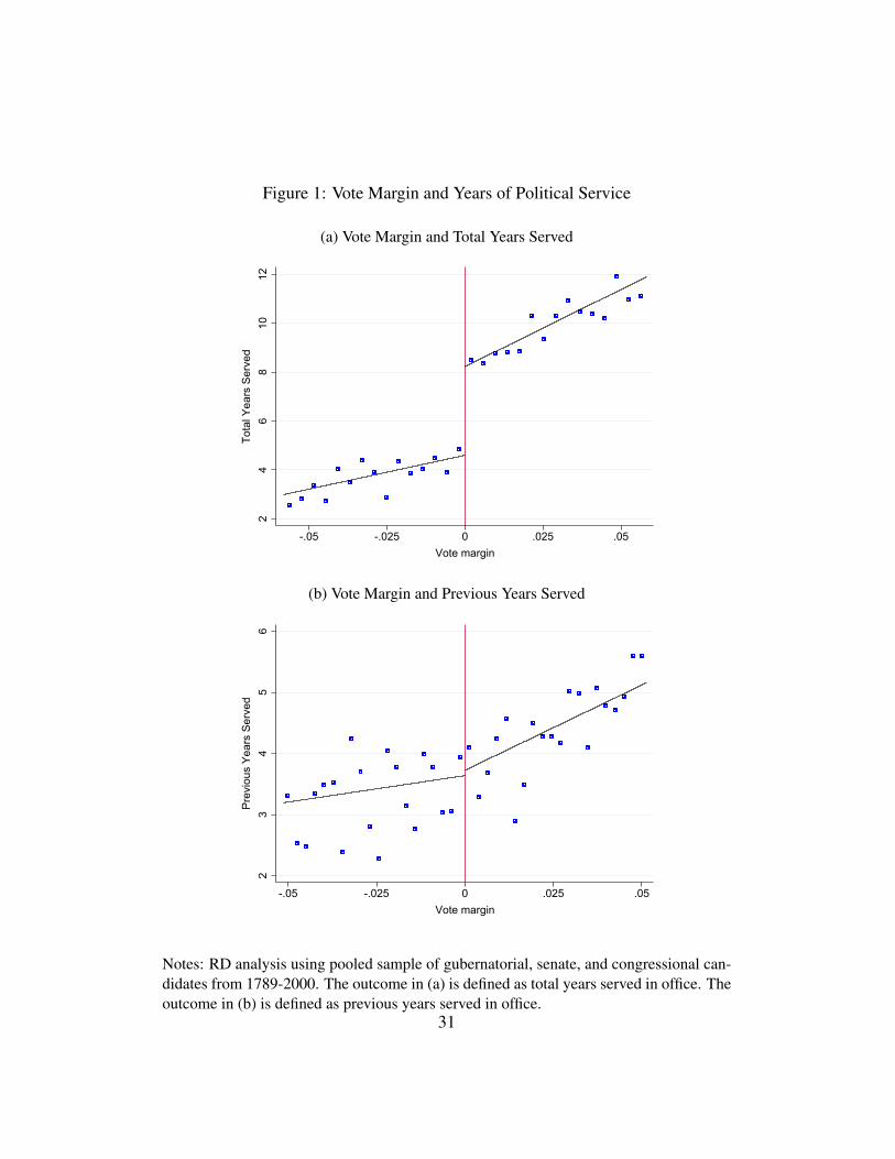
Figure 1: Vote Margin and Years of Political Service

(a) Vote Margin and Total Years Served

24

68

1012

Tota

l Yea

rs S

erve

d

-.05 -.025 0 .025 .05Vote margin

(b) Vote Margin and Previous Years Served

23

45

6Pr

evio

us Y

ears

Ser

ved

-.05 -.025 0 .025 .05Vote margin

Notes: RD analysis using pooled sample of gubernatorial, senate, and congressional can-didates from 1789-2000. The outcome in (a) is defined as total years served in office. Theoutcome in (b) is defined as previous years served in office.

31

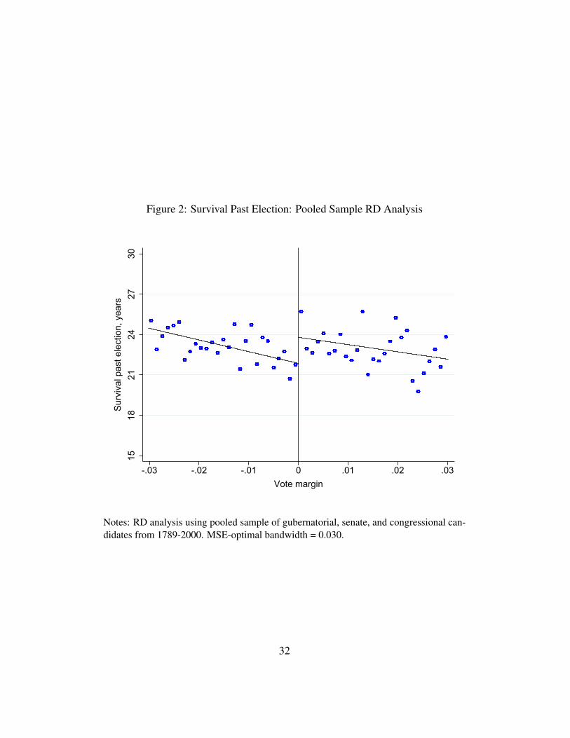
Figure 2: Survival Past Election: Pooled Sample RD Analysis

1518

2124

2730

Surv

ival

pas

t ele

ctio

n, y

ears

-.03 -.02 -.01 0 .01 .02 .03Vote margin

Notes: RD analysis using pooled sample of gubernatorial, senate, and congressional can-didates from 1789-2000. MSE-optimal bandwidth = 0.030.

32

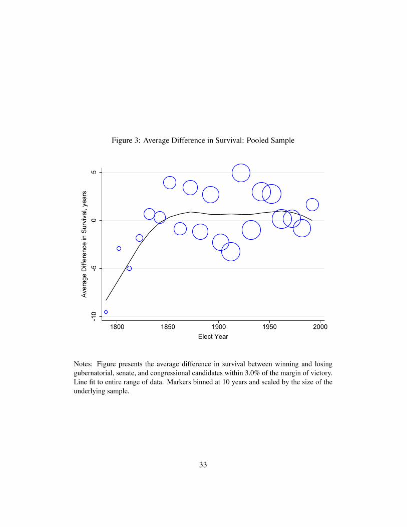
Figure 3: Average Difference in Survival: Pooled Sample

-10

-50

5Av

erag

e D

iffer

ence

in S

urvi

val,

year

s

1800 1850 1900 1950 2000Elect Year

Notes: Figure presents the average difference in survival between winning and losinggubernatorial, senate, and congressional candidates within 3.0% of the margin of victory.Line fit to entire range of data. Markers binned at 10 years and scaled by the size of theunderlying sample.

33

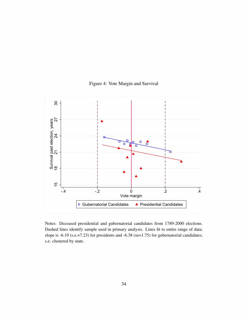
Figure 4: Vote Margin and Survival

1518

2124

2730

Surv

ival

pas

t ele

ctio

n, y

ears

-.4 -.2 0 .2 .4Vote margin

Gubernatorial Candidates Presidential Candidates

Notes: Deceased presidential and gubernatorial candidates from 1789-2000 elections.Dashed lines identify sample used in primary analysis. Lines fit to entire range of data;slope is -6.19 (s.e.=7.23) for presidents and -6.38 (se=1.75) for gubernatorial candidates;s.e. clustered by state.

34

Table 1: Summary Statistics: Age at Election and Death

Average SD NPooled

Age At Election 50.31 9.77 5711Winners Age At Election 50.27 9.75 3326Losers Age At Election 50.38 9.81 2385

Difference between winners and losers: 0.11 (p-value: 0.68 )Age At Death 73.32 11.89 5711Winners Age At Death 73.30 11.81 3326Losers Age At Death 73.36 12.01 2385

GovernorsAge At Election 50.24 9.02 2532Winners Age At Election 50.46 8.88 1290Losers Age At Election 50.00 9.16 1242

Difference between winners and losers: 0.46 (p-value: 0.20 )Age At Death 73.44 11.88 2532Winners Age At Death 73.46 11.98 1290Losers Age At Death 73.41 11.79 1242

SenatorsAge At Election 54.97 9.52 687Winners Age At Election 55.89 9.28 346Losers Age At Election 54.03 9.69 341

Difference between winners and losers: 1.85** (p-value: 0.01 )Age At Death 78.48 10.95 687Winners Age At Death 78.72 10.94 346Losers Age At Death 78.24 10.96 341

RepresentativesAge At Election 49.90 10.04 4523Winners Age At Election 49.83 9.93 2923Losers Age At Election 50.02 10.25 1600

Difference between winners and losers: 0.19 (p-value: 0.55 )Age At Death 72.73 11.88 4523Winners Age At Death 72.85 11.69 2923Losers Age At Death 72.51 12.23 1600

Notes: Summary statistics of age at election and death for gubernatorial, senate, andcongressional candidates who are within the relevant MSE-optimal bandwidth of eachsample. Candidates that are still alive or who died of accidents, assassinations, and otherviolent causes treated as censored observations. *, **, *** indicate significance levels of.10, .05, and .01, respectively.

35

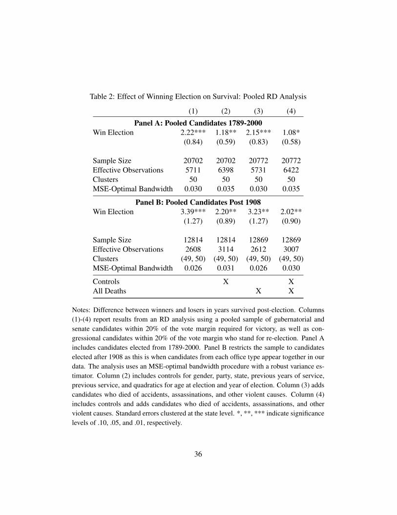
Table 2: Effect of Winning Election on Survival: Pooled RD Analysis

(1) (2) (3) (4)

Panel A: Pooled Candidates 1789-2000Win Election 2.22*** 1.18** 2.15*** 1.08*

(0.84) (0.59) (0.83) (0.58)

Sample Size 20702 20702 20772 20772Effective Observations 5711 6398 5731 6422Clusters 50 50 50 50MSE-Optimal Bandwidth 0.030 0.035 0.030 0.035

Panel B: Pooled Candidates Post 1908Win Election 3.39*** 2.20** 3.23** 2.02**

(1.27) (0.89) (1.27) (0.90)

Sample Size 12814 12814 12869 12869Effective Observations 2608 3114 2612 3007Clusters (49, 50) (49, 50) (49, 50) (49, 50)MSE-Optimal Bandwidth 0.026 0.031 0.026 0.030

Controls X XAll Deaths X X

Notes: Difference between winners and losers in years survived post-election. Columns(1)-(4) report results from an RD analysis using a pooled sample of gubernatorial andsenate candidates within 20% of the vote margin required for victory, as well as con-gressional candidates within 20% of the vote margin who stand for re-election. Panel Aincludes candidates elected from 1789-2000. Panel B restricts the sample to candidateselected after 1908 as this is when candidates from each office type appear together in ourdata. The analysis uses an MSE-optimal bandwidth procedure with a robust variance es-timator. Column (2) includes controls for gender, party, state, previous years of service,previous service, and quadratics for age at election and year of election. Column (3) addscandidates who died of accidents, assassinations, and other violent causes. Column (4)includes controls and adds candidates who died of accidents, assassinations, and otherviolent causes. Standard errors clustered at the state level. *, **, *** indicate significancelevels of .10, .05, and .01, respectively.

36

Table 3: Effect of Winning Election on Survival: RD Analysis by Office Type

Governors Senators Representatives(1789-2000) (1908-1994) (1823-1994)

(1) (2) (3) (4) (5) (6) (7) (8)

Win Election 1.15 1.63* 1.45* 1.42 1.37 -0.02 1.86* 0.77(1.08) (0.85) (0.83) (2.25) (1.97) (2.04) (1.00) (0.80)

Sample Size 4393 4393 4429 1784 1784 1818 14525 14525Effective Observations 2532 1987 2126 687 712 733 4523 5803Controls X X X X XAll Deaths X XClusters 50 50 50 48 48 48 (49, 50) (49, 50)MSE-Optimal Bandwidth 0.056 0.041 0.044 0.039 0.041 0.041 0.040 0.052

Notes: Difference between winners and losers in years survived post-election. Columns (1)-(3)report results for gubernatorial candidates in 1789-2000 within 20% of the margin required for vic-tory. Columns (4)-(6) report results for senate candidates in 1908-1994 within 20% of the marginrequired for victory. Columns (7)-(8) report results for representatives who stand for re-election in1823-1994. Each specification uses a MSE-optimal bandwidth with a robust variance estimator.Columns (2), (3), (5), (6), and (8) include controls for gender, party, state, previous service, andquadratics for age at election and year of election. Columns (3) and (6) adds candidates who diedof accidents, assassinations, and other violent causes. *, **, *** indicate significance levels of.10, .05, and .01, respectively.

37

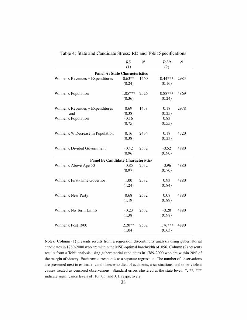
Table 4: State and Candidate Stress: RD and Tobit Specifications

RD N Tobit N(1) (2)

Panel A: State CharacteristicsWinner x Revenues + Expenditures 0.63** 1460 0.44*** 2983

(0.24) (0.16)

Winner x Population 1.05*** 2526 0.88*** 4869(0.36) (0.24)

Winner x Revenues + Expenditures 0.69 1458 0.18 2978and (0.38) (0.25)

Winner x Population -0.16 0.83(0.75) (0.55)

Winner x % Decrease in Population 0.16 2434 0.18 4720(0.38) (0.23)

Winner x Divided Government -0.42 2532 -0.52 4880(0.96) (0.90)

Panel B: Candidate CharacteristicsWinner x Above Age 50 -0.85 2532 -0.96 4880

(0.97) (0.70)

Winner x First-Time Governor 1.00 2532 0.93 4880(1.24) (0.84)

Winner x New Party 0.68 2532 0.08 4880(1.19) (0.89)

Winner x No Term Limits -0.23 2532 -0.20 4880(1.38) (0.98)

Winner x Post 1900 2.20** 2532 1.76*** 4880(1.04) (0.63)

Notes: Column (1) presents results from a regression discontinuity analysis using gubernatorialcandidates in 1789-2000 who are within the MSE-optimal bandwidth of .056. Column (2) presentsresults from a Tobit analysis using gubernatorial candidates in 1789-2000 who are within 20% ofthe margin of victory. Each row corresponds to a separate regression. The number of observationsare presented next to estimate. candidates who died of accidents, assassinations, and other violentcauses treated as censored observations. Standard errors clustered at the state level. *, **, ***indicate significance levels of .10, .05, and .01, respectively.

38

APPENDIX: FOR ONLINEPUBLICATION

A Previous Literature on Life Expectancy of Political Candi-

dates

The first article formalizing the study of the life expectancy of politicians appeared

in Metropolitan Statistical Bulletin in 1946. The Bulletin continued this line of

research for the next 4 decades, beginning a 1976 article on the longevity of US

presidents:

This year, as is usual in an election year, there has been renewed inter-

est in the question of the effect on longevity of the burdens of office

in what has been described as the world’s most demanding job —

President of the United States.

Here, we discuss the literature on politicians who served as president, governor or

head of government.29 The methods and conclusions of this research are summa-

rized in Tables 1a and 1b.

Early articles in this area, written between 1946 and 1980 and summarized in

Table 1a, generally compared presidents or governors to historical life tables. In

other words, adjustment was made for the expected survival of the candidate for

29 We should note that pre-1980 articles were somewhat difficult to uncover. Additional papersmay exist, especially in these earlier years.

their cohort of birth and age at election.30 This method often found that presidents

experienced shorter lives than expected. The first mention of the use of losing

candidates as the counterfactual appears in a 1973 Perspectives in Biology and

Medicine letter to the editor written by economist, journalist and author Nathaniel

Weyl. This was followed by several other comparisons of presidents (and some-

times vice-presidents, too) to unsuccessful candidates. This line of work con-

cluded that losing candidates outlived presidents, except in the case of the 1980

MetLife paper, which first adjusted for expected survival using a life table. Stan-

dard errors or confidence intervals are not reported in any of these papers.

More recently, the literature on the longevity of political executives has taken

a turn through the pages of the Journal of the American Medical Association,

American Sociological Review, and British Medical Journal; these papers are

summarized in Table 1b. Shavelle et al. (2008) and Olshansky (2011) update the

previous strategy of the MetLife Bulletin, using historical lifetables to compare

the longevity of US presidents to other men of their age and cohorts. Olshansky

(2011) finds that deceased presidents have survived slightly fewer years than ex-

pected; however, all surviving presidents have exceeded expected survival. On

the basis of this evidence, he concludes that presidential service does not reduce

life expectancy. Borgschulte (2014) points out that presidents are highly selected,

and the comparison to the general population ignores many factors which would

predict a longer life. Borgschulte uses a counterfactual of losing presidential can-

30 In general, it is unclear exactly which life tables were used in most of the papers. Presumably,the MetLife papers use tables maintained by the company for actuarial purposes.

40

didates, and find that presidents suffer a lost year of life for each year of service,

a difference which is statistically significant in most specifications. Link et al.

(2013) performs a similar analysis, combining presidents and vice-presidents in

their analysis of deaths from natural causes, finding that losing candidates ex-

hibit lower mortality risk than successful candidates. Most recently, Olenski et al.

(2015) compares the longevity of heads of state to losing electoral candidates,

finding similar, large losses to executive service. In sum, recent work using unsuc-

cessful candidates to estimate counterfactuals has found negative and significant

effects associated with service, with most estimates in the range of 1 year of life

lost for each year of service.

The study of the health effects of executive service is closely related to a

broader set of papers documenting the life expectancy of other groups of promi-

nent people. This literature is discussed in Borgschulte (2014) and Link et al.

(2013). Interested readers are referred to those papers.

A.1 Relationship to the Current Study

The primary problem in the identification of the causal effect of executive ser-

vice on longevity is the estimation of the counterfactual — how long would the

candidate have lived, absent election to office. The naive comparison of elected

executives to members of the unelected population—as in the life tables method—

combines the causal effect of service with the bias inherent in the non-random

selection into candidacy. As discussed by a number of papers in this literature, the

natural assumption is that elected executives are healthier than the general popu-

41

lation, given the robust findings of a large socio-economic gradient in health and

mortality for the last several hundred years.31 We can “solve” this problem (or at

least, greatly reduce the bias) by estimating counterfactual life expectancy using

a population of other privileged individuals drawn from the same time period and

social standing as the politicians. With this in mind, previous research has focused

on losing candidates as representative of the counterfactual population.

Despite the apparent improvement represented by the use of unsuccessful can-

didates to estimate the counterfactual, the comparison of winning and losing can-

didates may replace rather than resolve the selection problem. The selection

question now becomes whether electoral success, conditional on nomination to

the final round of balloting, is effectively unrelated to the life expectancy of the

candidates. Borgschulte (2014) discusses this issue in terms of “class versus grit”:

general election voters may prefer the candidate with some connection to the com-

mon man (grit), rather than the candidate with the highest social status (class).

If this is the case, then the comparison of winners to losers is biased towards a

negative effect of service. However, as healthier candidates possess many direct

advantages in campaigning, and research has documented a preference for healthy

leaders, previous work has proceeded with the assumption of an electoral bias for

healthier candidates.

A specific variation of the class versus grit issue emerges when comparing

incumbent or experienced candidates to electoral runners-up. If voters give sig-

31This bias is likely to grow with age, as older candidates will be evaluated for predictors ofshorter life expectancy in ways that younger candidates will not. This problem is discussed inBorgschulte (2014), and calls into question the use of life tables, even in a supplementary role.

42

nificant positive consideration to experience, then the weight placed on the candi-

date’s health may decline; experience may “crowd-out” health in the electorate’s

preferences.32 This issues is particularly salient in Olenski et al. (2015), which in-

cludes only the final electoral victory of heads-of-state in the sample, effectively

selecting a sample of politicians who are likely to have a non-longevity character-

istic (experience) which may crowd out the electoral preference for health. One

solution to this problem is the inclusion of controls for previous service. Con-

trolling for previous service will be an imperfect solution if what is preferred by

voters is not experience, but a willingness to sacrifice health and longevity in the

process of service (i.e. voters prefer a certain “type” of experienced candidate).

However, it is certainly preferable to control for previous experience, and dubious

to remove from the sample all but the final appearance or victory of the successful

candidates.

Behind these methodological issues lies a central obstacle: previous studies

have suffered from small sample sizes, preventing the direct assessment of their

assumptions and robustness to alternatives. Thus, the first contribution of this

paper to the literature is the sample size to test various assumptions.

B Data Appendix

A great deal of the biographical information for each candidate was found with

valuable help provided by research assistants (RAs). The RAs were given di-

32 This re-phrases the class versus grit issue to one of youth versus experience. Consider, forexample, the quite ill FDR, who was re-elected in 1944 on the basis of his experience in office.

43

rections to find birth and death dates for each candidate, gender, cause of death

(coded as violent/accidental or non-violent/non-accidental), primary occupation,

and birth state. Ideally, exact birth and death dates (day/month/year) were to be

coded. If the day of birth/death could not be found, we imputed the middle day of

the month of birth/death. If the day and month of birth/death could not be found,

we imputed the month and day to be July 2, the middle day of the year. For mem-

bers of congress we use only birth and death year. This was the format in which

we obtained the data and the large sample size prevented us from finding exact

birth/death dates for these candidates.

The RAs were instructed to use only creditable online or text resources. If the

candidate was found to still be alive, the RAs were instructed to note this under

a separate alive variable as well as indicate and cite the most recent date that the

candidate was known to still be living. For instances where cause of death was

not found, which in most cases occurred when searching for candidates who ran

for governor or senator in early years, we code the cause of death as being non-

violent/non-accidental.

By far the most challenging sourcing was data on the birth and death dates

of the losing candidates. Each of these candidates required an individual search,

with a research assistant instructed to record the source of the (usually online)

information. Dubin (2010) and Dubin (2013) provide first names for gubernatorial

candidates. In the best cases, the losing candidate was already in the dataset as

the winner of another election, in which case they could be either matched to their

biographical information in Glashan, or found on the webpage of the National

44

Governors’ Association. Similarly, candidates who served in the U.S. congress

appear in the Biographical Directory of the United States Congress, accessible at

bioguide.congress.gov. After these convenient sources were exhausted, a more

diverse set of online sources was used.

Political Graveyard is a website that tracks the life and death of US politi-

cians, and appears frequently in the sources. Find A Grave (findagrave.com) is a

website which photographs tombstones, and allows family members to enter bio-

graphical information about their loved ones. Google Books contains many books

that detail the history of individual states, such as “A History of Kentucky and

Kentuckians,” written by E. Polk Johnson and published in 1912. In some cases,

family genealogical records were required, accessible on the public portions of

Ancestry.com and Genealogy.com. In many cases, newspaper or election records

could supply crucial identifying information, such as the candidate’s wife’s name,

an unusual middle name or a date of birth, which could then be used to locate and

verify information regarding the candidate’s death. In a number of cases in early

US history, only a year or year and month of birth is available. In these cases, the

midpoint of the missing values is assumed.33

One concern with this type of project is that candidates who cannot be located

in the search have different life expectancies than those who are located. For this

sample, the potential bias is quite small. As well, the estimates are very similar

when using a more narrow window (i.e. 40-60%), where we found almost all

candidates.33The data and sources used in the paper will be posted at the time of publication.

45

The following presents details on the sources of supplementary state-level

data and variable construction:

State Population

The majority of the state population data was obtained from Population of States

and Counties of the United States: 1790-1990 (Forstall, 1996). Published in

1996 by the US Census Bureau, this report provides the populations of states

according to the twenty-one decennial U.S. censuses conducted from 1790 to

1990. Population data for the years 1990 and 2000 were obtained from individual

decennial censuses from the US Census Bureau. Population data is not available

for a very small number of observations where a gubernatorial election decided

by popular vote had taken place prior to there being an official state census. The

population variable used in our analysis is divided by 100,000 and logged. To

construct the variable for percent-change in population, we calculate the percent

change in population for each state using the state population 10 years prior.

Term Limits

Term Limit data was obtained from multiple sources, including Beasley and Case

(1995), Alt et al. (2011), and www.ballotpedia.org. Beasley and Case provide

governor term limits for each state for the years 1950 through 1986. Alt et al.

provide similar data that has been updated to include the years 1950 through

2000. The web resource www.ballotpedia.org proved very useful for obtaining

46

term limit data for the years prior to 1950. The website provides term limits

for each state along with citations from each state‘s constitutional amendment

that was created when a term limit was introduced or changed. The variable for

term limits is constructed as an indicator that takes the value 1 if a candidate is

prevented from running during the following Governor election due to state term

limit laws, and 0 otherwise. We then construct an interaction variable between

the term limit variable and the indicator variable for the winner of each election.

Expenditures and Revenues

State expenditure and revenue data was obtained from 3 sources. For early years,

we used the compiled dataset Sources and Uses of Funds in State and Local Gov-

ernments, 1790-1915 (Sylla et al., 1991). This dataset is available through ICPSR.

Total nominal revenue and expenditure data is available for the majority of years

and states from 1790 through 1915 (in some states the data is provided past 1915).

For later years, we combine data obtained directly from the US Census Bureau as

well as through the Urban Institute (available at taxpolicycenter.org). We adjust

the data to real terms ($ 2015) using the annual Consumer Price Index (available

at www.measuringworth.com).

A challenge was presented in creating relevant variables from the expenditure

and revenue data due to the candidate data being constructed at the election-year

level. Our strategy was to create variables that take into account revenue and

expenditure information over the course of all the years of a term, as opposed

to aggregate variables at the term level. To create a size of government variable

47

for each candidate, we sum annual real expenditures with annual real revenues

for each year of a particular term and average that amount across those years.

This gives us an approximate measure of the size of government for each year a

governor was in office. We then log this variable for our analysis. The variable for

fiscal deficits is constructed as a binary variable that takes the value 1 if over the

course of the years of a term, average annual total expenditures exceed average

annual total revenues, and 0 otherwise.

Divided Governments

We construct the variable for whether the governor experienced a divided govern-

ment using data obtained from Historical Party Affiliations of State Legislatures,

1796-2006, Dubin (2007). This resource contains state by state listings of the

party makeup for each state‘s legislature for every year since partisan contests

began and party affiliations were listed. The variable for divided government is

constructed as a binary variable that, for each candidate, takes the value 1 if at

least one of the state’s legislative body (House or Senate) was controlled by a

party that differs from the candidate‘s own party for the term years under consid-

eration, and 0 otherwise. Cases where control in a single legislative body is split

between two or more parties were coded as being divided. We then construct an

interaction variable between the divided government indicator and the indicator

variable for the winner of each election.

48

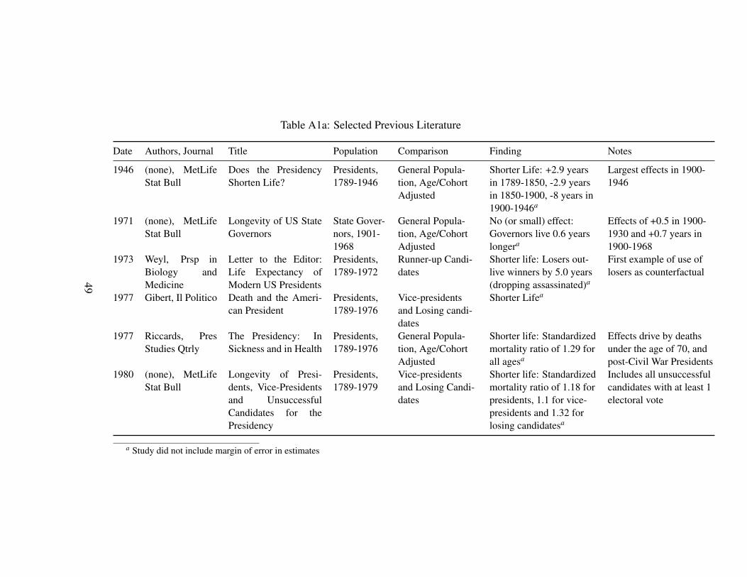
Table A1a: Selected Previous Literature

Date Authors, Journal Title Population Comparison Finding Notes

1946 (none), MetLifeStat Bull

Does the PresidencyShorten Life?

Presidents,1789-1946

General Popula-tion, Age/CohortAdjusted

Shorter Life: +2.9 yearsin 1789-1850, -2.9 yearsin 1850-1900, -8 years in1900-1946a

Largest effects in 1900-1946

1971 (none), MetLifeStat Bull

Longevity of US StateGovernors

State Gover-nors, 1901-1968

General Popula-tion, Age/CohortAdjusted

No (or small) effect:Governors live 0.6 yearslongera

Effects of +0.5 in 1900-1930 and +0.7 years in1900-1968

1973 Weyl, Prsp inBiology andMedicine

Letter to the Editor:Life Expectancy ofModern US Presidents

Presidents,1789-1972

Runner-up Candi-dates

Shorter life: Losers out-live winners by 5.0 years(dropping assassinated)a

First example of use oflosers as counterfactual

1977 Gibert, Il Politico Death and the Ameri-can President

Presidents,1789-1976

Vice-presidentsand Losing candi-dates

Shorter Lifea

1977 Riccards, PresStudies Qtrly

The Presidency: InSickness and in Health

Presidents,1789-1976

General Popula-tion, Age/CohortAdjusted

Shorter life: Standardizedmortality ratio of 1.29 forall agesa

Effects drive by deathsunder the age of 70, andpost-Civil War Presidents

1980 (none), MetLifeStat Bull

Longevity of Presi-dents, Vice-Presidentsand UnsuccessfulCandidates for thePresidency

Presidents,1789-1979

Vice-presidentsand Losing Candi-dates

Shorter life: Standardizedmortality ratio of 1.18 forpresidents, 1.1 for vice-presidents and 1.32 forlosing candidatesa

Includes all unsuccessfulcandidates with at least 1electoral vote

a Study did not include margin of error in estimates

49

Table A1b: Selected Previous Literature

Date Authors, Journal Title Population Comparison Finding Notes

2008 Shavelle, J Insur-ance Med

Underwriting thePresidents

Presidents,1789-2007

General Popula-tion, Age/CohortAdjusted

No effect: Standardizedmortality ratio of 1.07(95% CI: 0.76, 1.47)

Significantly shorter lifefor presidents elected in1845-1929 period

2011 Olshansky, Jof Amer MedAssoc

Aging of US Presi-dents

Presidents,1789-2009

General Popula-tion, Age/CohortAdjusted

No effect: Deceased pres-idents die 0.3 years ear-liera

Notes that living presi-dents have all exceededexpected survival

2014 Borgschulte,Unpub Mimeo

The Effect of Pres-idential Service onLife Expectancy

Presidents,1789-2012

Runner-up Candi-dates

Shorter life: CensoredTobit effect of -3.8 years(95%CI: -0.1, 7.5)

2014 Link et al, AmerSocio Review

Can Honorific AwardsGive Us Clues aboutthe Connection be-tween SocioeconomicStatus and Mortality?

Pres andVPs, 1789-2013

Runner-up Candi-dates

Shorter life: Hazardmodel effect of 1.53(p < 0.1) for naturalcauses, 1.66 for all causes(p < 0.05)

Combined sample ofpresidents and vice-presidents

2015 Olenski et al,Brit Med Journal

Do heads of gov-ernment age morequickly? Observa-tional study compar-ing mortality betweenelected leaders andrunners-up in nationalelections of 17 coun-tries

Heads ofgov’t, 1740-2015

Runner-up Candi-dates

Shorter life: Hazardmodel effect of 1.23(95% confidence inter-val 1.00 to 1.52) for all;loss of 2.7 years of life(95% CI from 0.6 to 4.8)for deceased

Does not drop assassi-nated subjects; drops allbut last election for win-ners

50

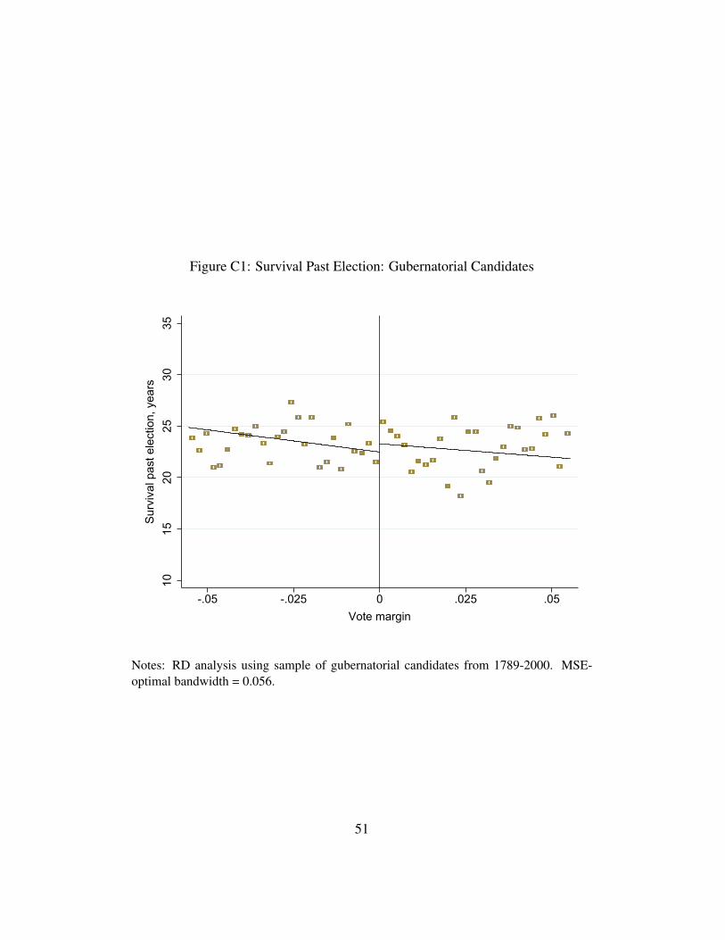
Figure C1: Survival Past Election: Gubernatorial Candidates

1015

2025

3035

Surv

ival

pas

t ele

ctio

n, y

ears

-.05 -.025 0 .025 .05Vote margin

Notes: RD analysis using sample of gubernatorial candidates from 1789-2000. MSE-optimal bandwidth = 0.056.

51

Figure C2: Survival Past Election: Senate Candidates

1520

2530

35Su

rviv

al p

ast e

lect

ion,

yea

rs

-.04 -.02 0 .02 .04Vote margin

Notes: RD analysis using sample of senate candidates from 1908-1994. MSE-optimalbandwidth = 0.039.

52

Figure C3: Survival Past Election: Congressional Candidates

1015

2025

30Su

rviv

al p

ast e

lect

ion,

yea

rs

-.04 -.02 0 .02 .04Vote margin

Notes: RD analysis using sample of congressional candidates from 1823-1994. MSE-optimal bandwidth = 0.040.

53

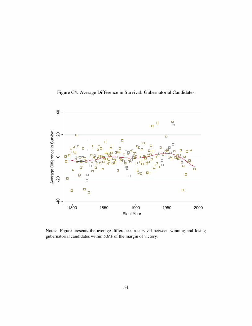
Figure C4: Average Difference in Survival: Gubernatorial Candidates

-40

-20

020

40Av

erag

e D

iffer

ence

in S

urvi

val

1800 1850 1900 1950 2000Elect Year

Notes: Figure presents the average difference in survival between winning and losinggubernatorial candidates within 5.6% of the margin of victory.

54

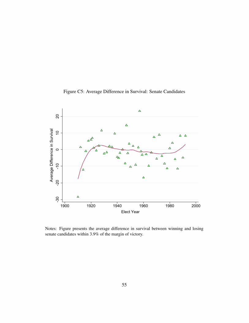
Figure C5: Average Difference in Survival: Senate Candidates

-30

-20

-10

010

20Av

erag

e D

iffer

ence

in S

urvi

val

1900 1920 1940 1960 1980 2000Elect Year

Notes: Figure presents the average difference in survival between winning and losingsenate candidates within 3.9% of the margin of victory.

55

Figure C6: Average Difference in Survival: Representatives

-20

-10

010

20Av

erag

e D

iffer

ence

in S

urvi

val

1800 1850 1900 1950 2000Elect Year

Notes: Figure presents the average difference in survival between winning and losingcongressional candidates within 4.0% of the margin of victory.

56

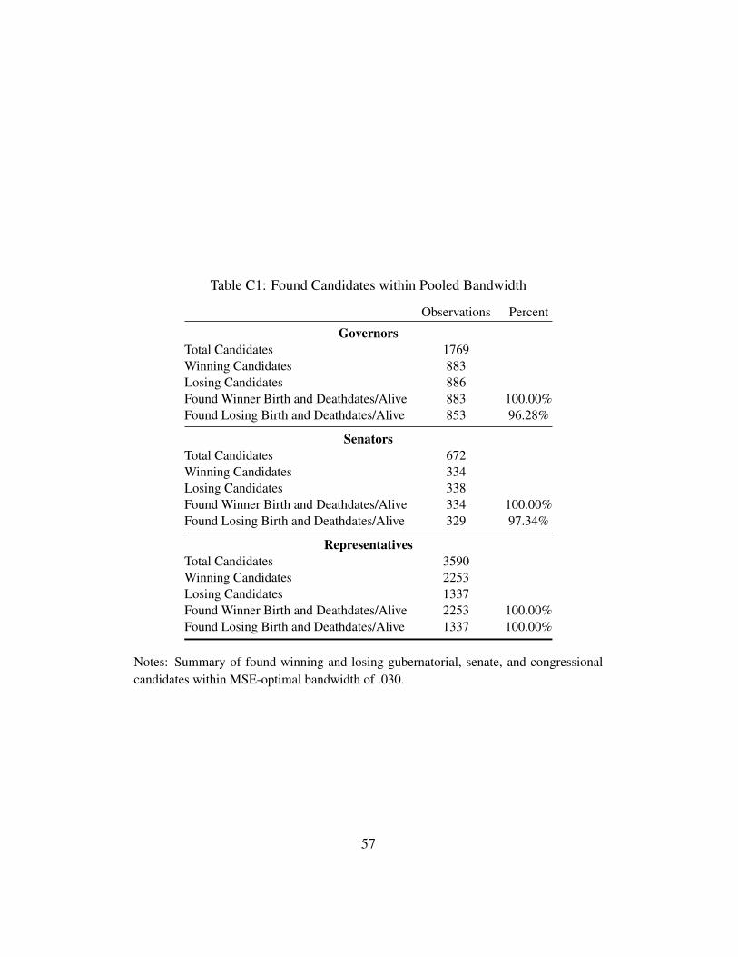
Table C1: Found Candidates within Pooled Bandwidth

Observations Percent

GovernorsTotal Candidates 1769Winning Candidates 883Losing Candidates 886Found Winner Birth and Deathdates/Alive 883 100.00%Found Losing Birth and Deathdates/Alive 853 96.28%

SenatorsTotal Candidates 672Winning Candidates 334Losing Candidates 338Found Winner Birth and Deathdates/Alive 334 100.00%Found Losing Birth and Deathdates/Alive 329 97.34%

RepresentativesTotal Candidates 3590Winning Candidates 2253Losing Candidates 1337Found Winner Birth and Deathdates/Alive 2253 100.00%Found Losing Birth and Deathdates/Alive 1337 100.00%

Notes: Summary of found winning and losing gubernatorial, senate, and congressionalcandidates within MSE-optimal bandwidth of .030.

57

Table C2: Found Candidates within 20% Margin

Observations Percent

GovernorsTotal Candidates 5155Winning Candidates 2513Losing Candidates 2642Found Winner Birth and Deathdates/Alive 2513 100.00%Found Losing Birth and Deathdates/Alive 2396 90.69%

SenatorsTotal Candidates 2367Winning Candidates 1185Losing Candidates 1182Found Winner Birth and Deathdates/Alive 1185 100.00%Found Losing Birth and Deathdates/Alive 1042 88.16%

RepresentativesTotal Candidates 16113Winning Candidates 13523Losing Candidates 2590Found Winner Birth and Deathdates/Alive 13523 100.00%Found Losing Birth and Deathdates/Alive 2590 100.00%

Notes: Summary of found winning and losing gubernatorial, senate, and congressionalcandidates who are within 20% of the margin of victory.

58

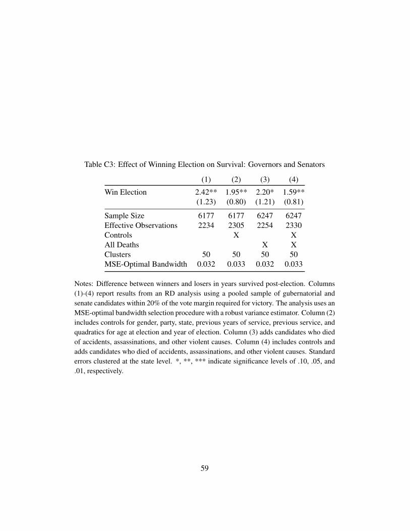
Table C3: Effect of Winning Election on Survival: Governors and Senators

(1) (2) (3) (4)

Win Election 2.42** 1.95** 2.20* 1.59**(1.23) (0.80) (1.21) (0.81)

Sample Size 6177 6177 6247 6247Effective Observations 2234 2305 2254 2330Controls X XAll Deaths X XClusters 50 50 50 50MSE-Optimal Bandwidth 0.032 0.033 0.032 0.033

Notes: Difference between winners and losers in years survived post-election. Columns(1)-(4) report results from an RD analysis using a pooled sample of gubernatorial andsenate candidates within 20% of the vote margin required for victory. The analysis uses anMSE-optimal bandwidth selection procedure with a robust variance estimator. Column (2)includes controls for gender, party, state, previous years of service, previous service, andquadratics for age at election and year of election. Column (3) adds candidates who diedof accidents, assassinations, and other violent causes. Column (4) includes controls andadds candidates who died of accidents, assassinations, and other violent causes. Standarderrors clustered at the state level. *, **, *** indicate significance levels of .10, .05, and.01, respectively.

59

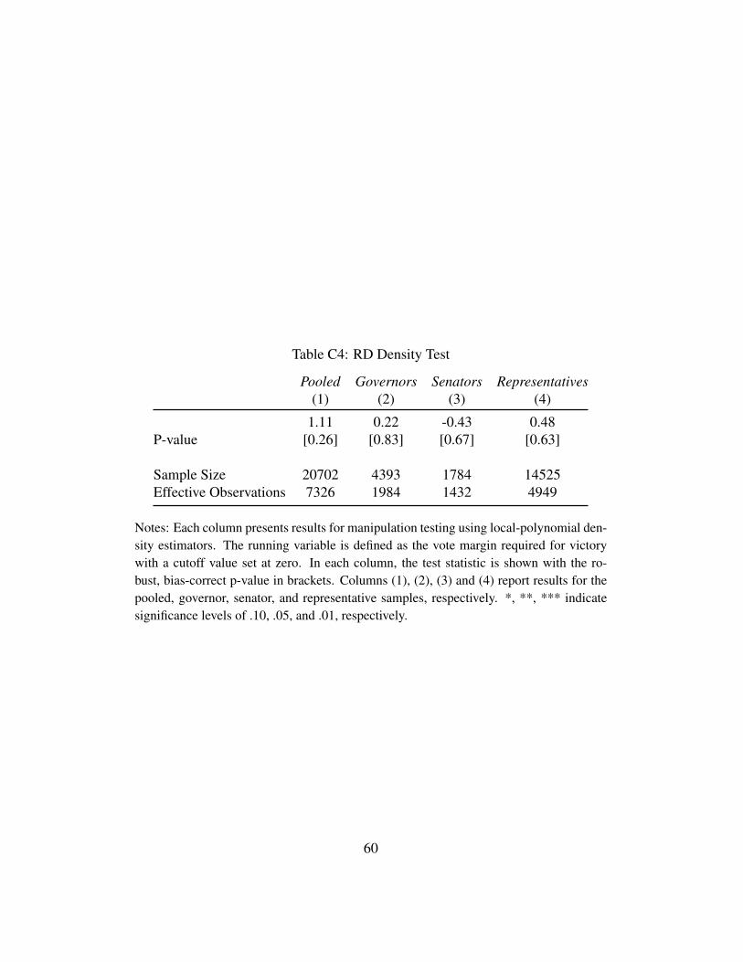
Table C4: RD Density Test

Pooled Governors Senators Representatives(1) (2) (3) (4)

1.11 0.22 -0.43 0.48P-value [0.26] [0.83] [0.67] [0.63]

Sample Size 20702 4393 1784 14525Effective Observations 7326 1984 1432 4949

Notes: Each column presents results for manipulation testing using local-polynomial den-sity estimators. The running variable is defined as the vote margin required for victorywith a cutoff value set at zero. In each column, the test statistic is shown with the ro-bust, bias-correct p-value in brackets. Columns (1), (2), (3) and (4) report results for thepooled, governor, senator, and representative samples, respectively. *, **, *** indicatesignificance levels of .10, .05, and .01, respectively.

60

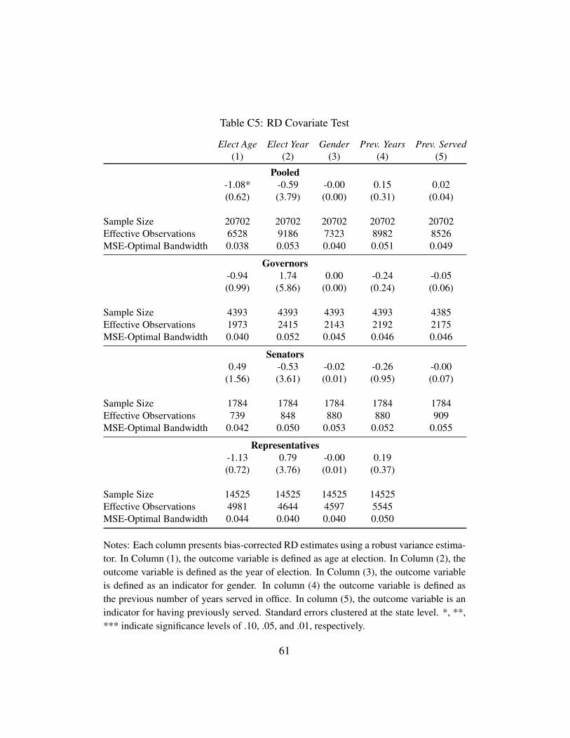
Table C5: RD Covariate Test

Elect Age Elect Year Gender Prev. Years Prev. Served(1) (2) (3) (4) (5)

Pooled-1.08* -0.59 -0.00 0.15 0.02(0.62) (3.79) (0.00) (0.31) (0.04)

Sample Size 20702 20702 20702 20702 20702Effective Observations 6528 9186 7323 8982 8526MSE-Optimal Bandwidth 0.038 0.053 0.040 0.051 0.049

Governors-0.94 1.74 0.00 -0.24 -0.05(0.99) (5.86) (0.00) (0.24) (0.06)

Sample Size 4393 4393 4393 4393 4385Effective Observations 1973 2415 2143 2192 2175MSE-Optimal Bandwidth 0.040 0.052 0.045 0.046 0.046

Senators0.49 -0.53 -0.02 -0.26 -0.00

(1.56) (3.61) (0.01) (0.95) (0.07)

Sample Size 1784 1784 1784 1784 1784Effective Observations 739 848 880 880 909MSE-Optimal Bandwidth 0.042 0.050 0.053 0.052 0.055

Representatives-1.13 0.79 -0.00 0.19(0.72) (3.76) (0.01) (0.37)

Sample Size 14525 14525 14525 14525Effective Observations 4981 4644 4597 5545MSE-Optimal Bandwidth 0.044 0.040 0.040 0.050

Notes: Each column presents bias-corrected RD estimates using a robust variance estima-tor. In Column (1), the outcome variable is defined as age at election. In Column (2), theoutcome variable is defined as the year of election. In Column (3), the outcome variableis defined as an indicator for gender. In column (4) the outcome variable is defined asthe previous number of years served in office. In column (5), the outcome variable is anindicator for having previously served. Standard errors clustered at the state level. *, **,*** indicate significance levels of .10, .05, and .01, respectively.

61

Table C6: Stressful State Characteristics: RD Analysis

Rev + Exp Population Rev/Exp + Pop Decrease in Pop Divided Govt.(1) (2) (3) (4) (5)

Winner 0.81 -0.20 0.78 0.08 0.05(1.03) (0.84) (1.04) (0.84) (1.03)

Win X Revenues + Expenditures 0.63** 0.69(0.24) (0.38)

Win X Population 1.05*** -0.16(0.36) (0.75)

Win X % Decrease in Population 0.16(0.38)

Win X Divided Government -0.42(0.96)

Observations 1460 2526 1458 2434 2532Controls X X X X XClusters 50 50 50 50 50

Notes: Results from RD analysis using Gubernatorial candidates in 1789-2000 who arewithin the MSE-optimal bandwidth of .056. Candidates who died of accidents, assassina-tions, and other violent causes are treated as censored observations. Column (1) includesan interaction between winner and the sum of state revenues and expenditures. Column(2) includes an interaction between winner and logged state population. Column (3) in-cludes an interaction between winner and the sum of state revenues and expenditures, andan interaction between winner and logged state population. Column (4) includes an in-teraction between winner and percent change in state population. Column (5) includes aninteraction between winner and an indicator for whether the winner experienced a dividedgovernment during a term in office. Standard errors clustered at the state level. *, **, ***indicate significance levels of .10, .05, and .01, respectively.

62

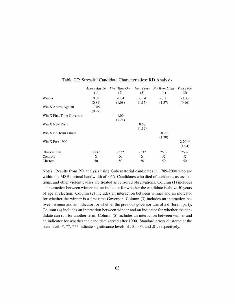
Table C7: Stressful Candidate Characteristics: RD Analysis

Above Age 50 First Time Gov New Party No Term Limit Post 1900(1) (2) (3) (4) (5)

Winner 0.09 -1.04 -0.54 - 0.11 -1.33(0.89) (1.08) (1.15) (1.37) (0.96)

Win X Above Age 50 -0.85(0.97)

Win X First Time Governor 1.00(1.24)

Win X New Party 0.68(1.19)

Win X No Term Limits -0.23(1.38)

Win X Post 1900 2.20**(1.04)

Observations 2532 2532 2532 2532 2532Controls X X X X XClusters 50 50 50 50 50

Notes: Results from RD analysis using Gubernatorial candidates in 1789-2000 who arewithin the MSE-optimal bandwidth of .056. Candidates who died of accidents, assassina-tions, and other violent causes are treated as censored observations. Column (1) includesan interaction between winner and an indicator for whether the candidate is above 50 yearsof age at election. Column (2) includes an interaction between winner and an indicatorfor whether the winner is a first time Governor. Column (3) includes an interaction be-tween winner and an indicator for whether the previous governor was of a different party.Column (4) includes an interaction between winner and an indicator for whether the can-didate can run for another term. Column (5) includes an interaction between winner andan indicator for whether the candidate served after 1900. Standard errors clustered at thestate level. *, **, *** indicate significance levels of .10, .05, and .01, respectively.

63

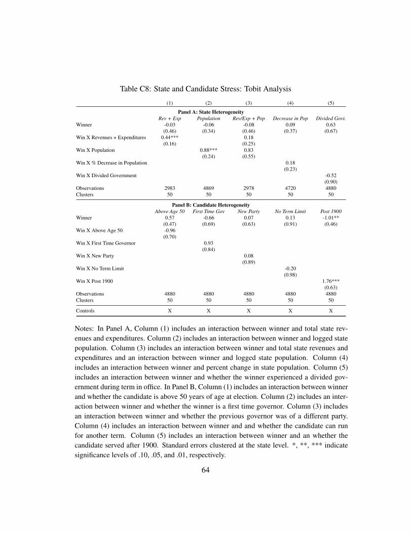
Table C8: State and Candidate Stress: Tobit Analysis

(1) (2) (3) (4) (5)

Panel A: State HeterogeneityRev + Exp Population Rev/Exp + Pop Decrease in Pop Divided Govt.

Winner -0.03 -0.06 -0.08 0.09 0.63(0.46) (0.34) (0.46) (0.37) (0.67)

Win X Revenues + Expenditures 0.44*** 0.18(0.16) (0.25)

Win X Population 0.88*** 0.83(0.24) (0.55)

Win X % Decrease in Population 0.18(0.23)

Win X Divided Government -0.52(0.90)

Observations 2983 4869 2978 4720 4880Clusters 50 50 50 50 50

Panel B: Candidate HeterogeneityAbove Age 50 First Time Gov New Party No Term Limit Post 1900

Winner 0.57 -0.66 0.07 0.13 -1.01**(0.47) (0.69) (0.63) (0.91) (0.46)

Win X Above Age 50 -0.96(0.70)

Win X First Time Governor 0.93(0.84)

Win X New Party 0.08(0.89)

Win X No Term Limit -0.20(0.98)

Win X Post 1900 1.76***(0.63)

Observations 4880 4880 4880 4880 4880Clusters 50 50 50 50 50

Controls X X X X X

Notes: In Panel A, Column (1) includes an interaction between winner and total state rev-enues and expenditures. Column (2) includes an interaction between winner and logged statepopulation. Column (3) includes an interaction between winner and total state revenues andexpenditures and an interaction between winner and logged state population. Column (4)includes an interaction between winner and percent change in state population. Column (5)includes an interaction between winner and whether the winner experienced a divided gov-ernment during term in office. In Panel B, Column (1) includes an interaction between winnerand whether the candidate is above 50 years of age at election. Column (2) includes an inter-action between winner and whether the winner is a first time governor. Column (3) includesan interaction between winner and whether the previous governor was of a different party.Column (4) includes an interaction between winner and and whether the candidate can runfor another term. Column (5) includes an interaction between winner and an whether thecandidate served after 1900. Standard errors clustered at the state level. *, **, *** indicatesignificance levels of .10, .05, and .01, respectively.

64