DISCUSSION PAPER SERIES

IZA DP No. 10802

Giuseppe ForteJonathan Portes

Macroeconomic Determinants of International Migration to the UK

MAY 2017

Any opinions expressed in this paper are those of the author(s) and not those of IZA. Research published in this series may include views on policy, but IZA takes no institutional policy positions. The IZA research network is committed to the IZA Guiding Principles of Research Integrity.The IZA Institute of Labor Economics is an independent economic research institute that conducts research in labor economics and offers evidence-based policy advice on labor market issues. Supported by the Deutsche Post Foundation, IZA runs the world’s largest network of economists, whose research aims to provide answers to the global labor market challenges of our time. Our key objective is to build bridges between academic research, policymakers and society.IZA Discussion Papers often represent preliminary work and are circulated to encourage discussion. Citation of such a paper should account for its provisional character. A revised version may be available directly from the author.

Schaumburg-Lippe-Straße 5–953113 Bonn, Germany

Phone: +49-228-3894-0Email: publications@iza.org www.iza.org

IZA – Institute of Labor Economics

DISCUSSION PAPER SERIES

IZA DP No. 10802

Macroeconomic Determinants of International Migration to the UK

MAY 2017

Giuseppe ForteKing’s College London

Jonathan PortesKing’s College London and IZA

ABSTRACT

MAY 2017IZA DP No. 10802

Macroeconomic Determinants of International Migration to the UK*

This paper examines the determinants of long-term international migration to the UK;

we explore the extent to which migration is driven by macroeconomic variables (GDP per

capita, unemployment rate) as well as law and policy (the existence of “free movement”

rights for EEA nationals). We find a very large impact from free movement within the

EEA. We also find that macroeconomic variables – UK GDP growth and GDP at origin –

are significant drivers of migration flows; evidence for the impact of the unemployment

rate in countries of origin, or of the exchange rate, however, is weak. We conclude that,

while future migration flows will be driven by a number of factors, macroeconomic and

otherwise, Brexit and the end of free movement will result in a large fall in immigration

from EEA countries to the UK.

JEL Classification: F22, J61, J68

Keywords: Brexit, EU, immigration, UK

Corresponding author:Jonathan PortesDepartment of Political EconomyKing’s College LondonStrand Campus London WC2R 2LSUnited Kingdom

E-mail: jonathan.portes@kcl.ac.uk

* This work was supported by Jonathan Portes’ Senior Fellowship of the UK in a Changing Europe programme, financed by the Economic and Social Research Council.

Contents

1 Introduction 1

2 Data: The International Passenger Survey 3

3 Theory 103.1 Grogger and Hanson (2011) and Beine et al. (2011) . . . . . . . . . . . 113.2 Ortega and Peri (2013) . . . . . . . . . . . . . . . . . . . . . . . . . . . 12

4 Results and Discussion 16

5 Improving immigration statistics 20

6 Conclusion 22

References 23

Annexes 27A National Insurance Registrations and IPS: a Comparison . . . . . . . . 27B List of countries analysed . . . . . . . . . . . . . . . . . . . . . . . . . . 29

List of Figures

1 Frequency of origin-year inflows, by magnitude . . . . . . . . . . . . . . 6A.1 Comparison of sources (from Office for National Statistics (2016c)) . . . 28

List of Tables

1 Migratory inflows by selected region and 4-year period (000’s) . . . . . 82 Summary statistics for main variables . . . . . . . . . . . . . . . . . . . 93 Regression estimates . . . . . . . . . . . . . . . . . . . . . . . . . . . . 18

i

1 Introduction

This paper examines the determinants of long-term international migration to the UK;

we explore the extent to which migration is driven by macroeconomic variables (GDP

per capita, unemployment rate) as well as law and policy (the existence of “free move-

ment” rights for EEA nationals). We focus on international migration as measured in

the International Passenger Survey (IPS), which is the main source for the Long-Term

International Migration (LTIM) series published by the Office for National Statistics

(ONS). LTIM is in turn the official measure of immigration to the UK, both for stat-

istical purposes and for the government’s target of reducing (net) immigration to the

“tens of thousands”1.

The use of the IPS has been much criticised by UK media and policymakers in re-

cent years (for instance, House of Commons (2013)) because of its alleged unreliability,

discussed in detail below. However, given its key role in the public and policy debate,

it is clearly important to examine whether it is possible to use IPS data to produce

meaningful analyses of the determinants of migration flows. In particular, there is a

vigorous political debate about whether Brexit will in fact make a significant contri-

bution to reducing migration, and in particular to hitting the government’s target, as

some argue (Migration Watch (2016)) or whether in fact immigration is driven primar-

ily by economic conditions, and largely unaffected by policy change (European Union

Committee (2017)).

Our analysis suggests that there are indeed serious issues with the use of the IPS

for the analysis of migration flows, particularly at a country level. The relatively small

sample sizes for long-term migrants, the discretionary nature of responses to the sur-1Home Secretary, HC Deb, 23 November 2010, col 169. URL: goo.gl/tck4H0

1

vey and various methodological changes (with associated revisions) over recent years

all introduce a considerable amount of noise and potential bias into the data. This

is clearly problematic from both a statistical perspective (given the use of the LTIM

figures for population estimates and projections) and from a policy one (since the of-

ficial government target for migration uses the net LTIM figure). Given the centrality

of immigration to the UK policy debate, both in the context of Brexit and beyond,

improvement (including much greater use of administrative data) is urgently required,

as the UK Statistics Authority has recently argued (UK Statistics Authority (2013a),

UK Statistics Authority (2013b); UK Statistics Authority (2016)).

Nevertheless, even given the data limitations, our analysis does produce meaningful

results, consistent both with theory and previous work. In particular:

• We find a very large impact from free movement within the EEA. Consistent

with our previous work using National Insurance number data (Portes and Forte

(2017)), we find that countries whose citizens have free movement rights see a

roughly six-fold increase in migration flows to the UK;

• We find that macroeconomic variables – in particular UK GDP per capita and

employment rate differential with country of origin – are significant drivers of

migration flows; evidence for the impact the unemployment rate in countries of

origin, or of the exchange rate, however, is weak.

We conclude that, as we argued previously (Portes and Forte (2017)), while future

migration flows will be driven by a number of factors, macroeconomic and otherwise,

Brexit and the end of free movement will result in a large fall in immigration from EEA

2

countries to the UK. As our earlier analysis showed, this is likely to have significant

negative impacts on the UK economy overall (in both GDP and GDP per capita terms),

while exerting only a very modest upward pressure on wages at the lower end of the

labour market.

The remainder of the paper is organised as follows: Section 2 presents the International

Passenger Survey and descriptive statistics for the 2000-2015 data; Section 3 presents a

theoretical model of international migration as well as our specification and estimator

of choice; in Section 4 we discuss our findings in relationship with the international

literature; Section 5 details briefly the necessity for improved immigration statistics;

Section 6 concludes and recapitulates the article.

2 Data: The International Passenger Survey

There is no one source of data on immigration to the UK. The Labour Force Sur-

vey (LFS) and the Annual Population Survey (APS) give information on the size,

demographics and labour market characteristics of the migrant population; the British

Household Panel Survey (BHPS) and, more recently, the UK Household Longitudinal

Study (Understanding Society) can be employed to analyse the dynamics of a broader

range of socio-economic characteristics of the immigrant sub-sample over time; the

Census gives much more detailed data on the resident population, but only once every

decade; and National Insurance Number (NINo) registrations have been used as prox-

ies for migrant inflows.

However, the Long Term International Migration (LTIM) estimates (Office for Na-

tional Statistics (2017)) are by far the most widely used as a measure of immigration,

emigration, and net migration; LTIM is in turn largely based on the IPS. The IPS

3

has been conducted by the ONS since 1961 to obtain information regarding incoming

(outgoing) travellers at their point of arrival (departure). The survey covers most im-

portant British airports and seaports, for a total coverage of around 95% of British

international passenger traffic, and identifies long-term migrants based on their de-

clared intention to change country of residence for at least a year (in line with United

Nations conventions).

The IPS does not account for passengers who change their mind about the length

of stay against their declared intentions, the so-called ‘migrant switchers’ (although ef-

forts are made to include their impact by imputing the importance of the phenomenon

using immigrants’ responses on their personal history). Moreover, it does not capture

immigrants crossing the Northern Ireland-EIRE border (Office for National Statistics

(2015a)), nor asylum-seekers. LTIM figures are the results of adjustments to include

estimates of ‘switchers’, asylum seekers and migrants from the Republic of Ireland.

On average, around 700000-800000 contacts take place every year, over 362 days from

6am to 10pm. In recent years, the number of individuals recorded as long-term mi-

grants has been ranging between 4000 and 5000 per annum2 (1 in 160-200 contacts at

selected borders), of which around 3000 immigrants and 1500-2000 emigrants.

Eight-stage weighting and seasonal adjustment are used to obtain nationally rep-

resentative statistics from the total number of IPS contacts; the number of long-term

immigrants are then obtained by further analysing the migration sub-sample of the

resulting total. That is, flow central values and confidence intervals are the results

of weighting applied to the entire IPS sample, plus specific weighting applied to the

5000 interviews with migrants. The survey methodology underwent significant changes2For comparison, 335500 interviews were used to produce Overseas Travel and Tourism estimates

in 2015 (Office for National Statistics (2016d)).

4

in 2009 in order to increase the statistical robustness for estimates of the number of

immigrants entering through airports other than Heathrow: while this caused minor

discontinuities between 2008 and 2009 immigration estimates, the magnitude of the

disruption is “no cause for concern” according to the ONS (Office for National Statist-

ics (2015a)).

Of more significant concern is the review of the 2001-2011 estimates that was con-

ducted by comparing IPS data with information from the 2011 Census. The published

follow-up document concludes that the IPS “missed a substantial amount of immigra-

tion of EU8 citizens that occurred between 2004 and 2008, prior to IPS improvements

in 2009” and it “underestimated the migration of children” (Office for National Statist-

ics (2014)); the number of working-age women is found to be severely under-reported as

well. This led the ONS to provide updated long-term international migration series for

the decade ending in 2011, with yearly corrections reaching 67000 immigrants mostly

relating to migration from the European Union. However, this update was only conduc-

ted for net migration, and at a high level of geographical aggregation, not for inflows

or outflows, nor at a country level. Office for National Statistics (2014, p. 56) states:

“Users who wish to see a more detailed breakdown of inflows and outflows [. . . ] by

variables such as reason for migration, age and sex, citizenship and country of birth

should continue to use the existing LTIM and IPS 1, 2 and 3 series tables, but should

bear in mind the caveat that the headline net migration estimates have now been revised

[. . . ]” (italics added). 3

3Note that this is not an isolated case: IPS estimates and methodology have historically beensubject to multiple revisions, a practice that inevitably hinders the credibility of the source for researchand policy use. For example, in addition to the 2009 discontinuity and the 2011 Census revision,another discontinuity between 1998 and 1999 measures resulted from changes to the measurement ofmigration to and from the Republic of Ireland (Office for National Statistics (2015b)).

5

In previous work (Portes and Forte (2017)), we used National Insurance number

registrations (by country and quarter) as a measure of migrant inflows. Annex A sets

out the key differences between the two data sources. For this study, we construct a

similar dataset using the IPS. Data for the dependent flow variable come from publicly

available ‘International Passenger Survey 4.06, country of birth by citizenship’ (Office

for National Statistics (2016b)) spreadsheets, which report yearly inflows by country

and relative confidence intervals.

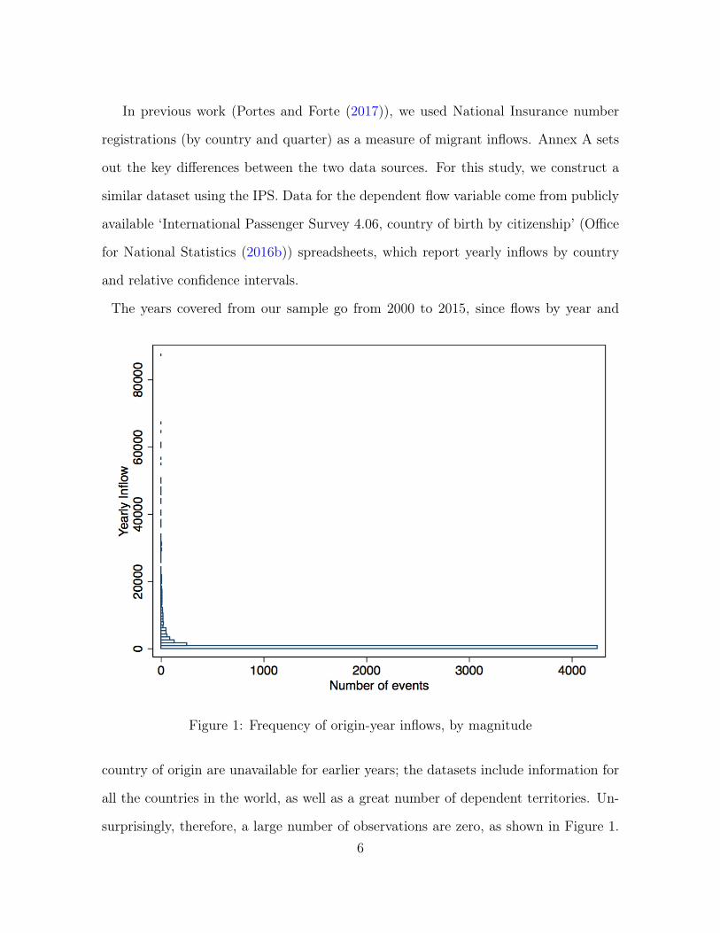
The years covered from our sample go from 2000 to 2015, since flows by year and

Figure 1: Frequency of origin-year inflows, by magnitude

country of origin are unavailable for earlier years; the datasets include information for

all the countries in the world, as well as a great number of dependent territories. Un-

surprisingly, therefore, a large number of observations are zero, as shown in Figure 1.6

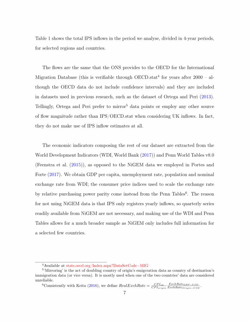
Table 1 shows the total IPS inflows in the period we analyse, divided in 4-year periods,

for selected regions and countries.

The flows are the same that the ONS provides to the OECD for the International

Migration Database (this is verifiable through OECD.stat4 for years after 2000 – al-

though the OECD data do not include confidence intervals) and they are included

in datasets used in previous research, such as the dataset of Ortega and Peri (2013).

Tellingly, Ortega and Peri prefer to mirror5 data points or employ any other source

of flow magnitude rather than IPS/OECD.stat when considering UK inflows. In fact,

they do not make use of IPS inflow estimates at all.

The economic indicators composing the rest of our dataset are extracted from the

World Development Indicators (WDI, World Bank (2017)) and Penn World Tables v8.0

(Feenstra et al. (2015)), as opposed to the NiGEM data we employed in Portes and

Forte (2017). We obtain GDP per capita, unemployment rate, population and nominal

exchange rate from WDI; the consumer price indices used to scale the exchange rate

by relative purchasing power parity come instead from the Penn Tables6. The reason

for not using NiGEM data is that IPS only registers yearly inflows, so quarterly series

readily available from NiGEM are not necessary, and making use of the WDI and Penn

Tables allows for a much broader sample as NiGEM only includes full information for

a selected few countries.

4Available at stats.oecd.org/Index.aspx?DataSetCode=MIG5‘Mirroring’ is the act of doubling country of origin’s emigcration data as country of destination’s

immigration data (or vice versa). It is mostly used when one of the two countries’ data are consideredunreliable.

6Consistently with Keita (2016), we define RealExchRate = CPIuk

CPIorigin

ExchRateGBP−USD

ExchRateOrigin−USD.

7

2000-2003 2004-2007 2008-2011 2012-2015

European Union 243.8 507.3 572.3 775.9

A2 8.3 16.6 40.5 135.9

A8 24.9 291.7 259.4 250.9

Rest of EU 210.6 199 272.4 389.1

Other Europe 15.4 26.6 24.8 37

Asia 382.4 635.6 771.1 586.6

China 89.3 69.4 113 168.7

India 57 209.2 241.4 148.1

Rest of Asia 236.1 357 416.7 269.8

North America 94.2 86.6 88.5 113.3

United States 59.7 59.6 52.4 66.8

Canada 22 15.1 26.5 30.2

Rest of North America 12.5 11.9 9.6 16.3

South America 14.7 21 23.9 24.1

Brazil 4.8 10.3 10.9 14.3

Oceania 136.4 110 59.7 72.8

Australia 94.6 67.5 44.9 58

Table 1: Migratory inflows by selected region and 4-year period (000’s)

8

VARIABLES N Mean St. Deviation Minimum Maximum

Origin-to-UK Migration 3,984 1.847 7.439 0 109.8

UK GDP per capita (2010 $) 3,984 38,887 1,664 35,250 41,188

Origin GDP per capita (2010$) 2,991 12,914 18,804 194.2 145,221

Origin Unemployment Rate (%) 2,595 8.678 6.178 0.100 38.60

Real Exchange Rate 2,407 0.255 0.394 1.04e-05 4.668

Free Movement 3,984 0.0921 0.289 0 1

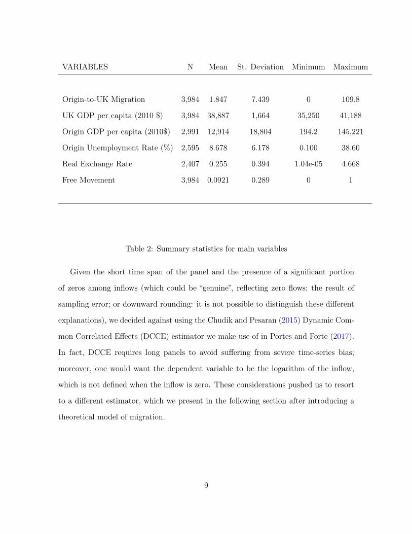
Table 2: Summary statistics for main variables

Given the short time span of the panel and the presence of a significant portion

of zeros among inflows (which could be “genuine”, reflecting zero flows; the result of

sampling error; or downward rounding: it is not possible to distinguish these different

explanations), we decided against using the Chudik and Pesaran (2015) Dynamic Com-

mon Correlated Effects (DCCE) estimator we make use of in Portes and Forte (2017).

In fact, DCCE requires long panels to avoid suffering from severe time-series bias;

moreover, one would want the dependent variable to be the logarithm of the inflow,

which is not defined when the inflow is zero. These considerations pushed us to resort

to a different estimator, which we present in the following section after introducing a

theoretical model of migration.

9

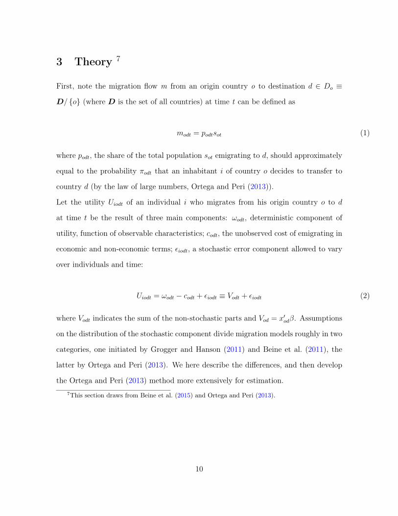
3 Theory 7

First, note the migration flow m from an origin country o to destination d ∈ Do ≡

D/ o (where D is the set of all countries) at time t can be defined as

modt = podtsot (1)

where podt, the share of the total population sot emigrating to d, should approximately

equal to the probability πodt that an inhabitant i of country o decides to transfer to

country d (by the law of large numbers, Ortega and Peri (2013)).

Let the utility Uiodt of an individual i who migrates from his origin country o to d

at time t be the result of three main components: ωodt, deterministic component of

utility, function of observable characteristics; codt, the unobserved cost of emigrating in

economic and non-economic terms; εiodt, a stochastic error component allowed to vary

over individuals and time:

Uiodt = ωodt − codt + εiodt ≡ Vodt + εiodt (2)

where Vodt indicates the sum of the non-stochastic parts and Vod = x′odβ. Assumptions

on the distribution of the stochastic component divide migration models roughly in two

categories, one initiated by Grogger and Hanson (2011) and Beine et al. (2011), the

latter by Ortega and Peri (2013). We here describe the differences, and then develop

the Ortega and Peri (2013) method more extensively for estimation.7This section draws from Beine et al. (2015) and Ortega and Peri (2013).

10

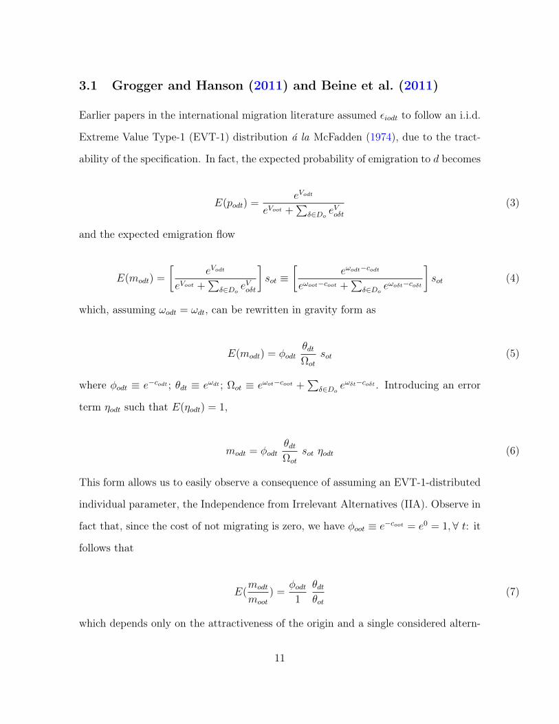
3.1 Grogger and Hanson (2011) and Beine et al. (2011)

Earlier papers in the international migration literature assumed εiodt to follow an i.i.d.

Extreme Value Type-1 (EVT-1) distribution á la McFadden (1974), due to the tract-

ability of the specification. In fact, the expected probability of emigration to d becomes

E(podt) =eVodt

eVoot +∑

δ∈Do eVoδt

(3)

and the expected emigration flow

E(modt) =

[eVodt

eVoot +∑

δ∈Do eVoδt

]sot ≡

[eωodt−codt

eωoot−coot +∑

δ∈Do eωoδt−coδt

]sot (4)

which, assuming ωodt = ωdt, can be rewritten in gravity form as

E(modt) = φodtθdtΩot

sot (5)

where φodt ≡ e−codt ; θdt ≡ eωdt ; Ωot ≡ eωot−coot +∑

δ∈Do eωδt−coδt . Introducing an error

term ηodt such that E(ηodt) = 1,

modt = φodtθdtΩot

sot ηodt (6)

This form allows us to easily observe a consequence of assuming an EVT-1-distributed

individual parameter, the Independence from Irrelevant Alternatives (IIA). Observe in

fact that, since the cost of not migrating is zero, we have φoot ≡ e−coot = e0 = 1,∀ t: it

follows that

E(modt

moot

) =φodt

1

θdtθot

(7)

which depends only on the attractiveness of the origin and a single considered altern-

11

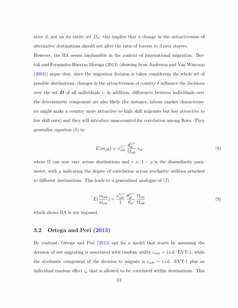
ative d, not on its entire set Do: this implies that a change in the attractiveness of

alternative destinations should not alter the ratio of leavers to d over stayers.

However, the IIA seems implausible in the context of international migration. Ber-

toli and Fernández-Huertas Moraga (2013) (drawing from Anderson and Van Wincoop

(2003)) argue that, since the migration decision is taken considering the whole set of

possible destinations, changes in the attractiveness of country δ influence the decisions

over the set D of all individuals i; in addition, differences between individuals over

the deterministic component are also likely (for instance, labour market characterist-

ics might make a country more attractive to high skill migrants but less attractive to

low skill ones) and they will introduce unaccounted-for correlation among flows. They

generalise equation (5) to

E(modt) = φ1/τodt

θ1/τdt

Ωodt

sot (8)

where Ω can now vary across destinations and τ ≡ 1 − ρ is the dissimilarity para-

meter, with ρ indicating the degree of correlation across stochastic utilities attached

to different destinations. This leads to a generalised analogue of (7)

E(modt

moot

) =φ1/τodt

1

θ1/τdt

θot

Ωoot

Ωodt

(9)

which shows IIA is not imposed.

3.2 Ortega and Peri (2013)

By contrast, Ortega and Peri (2013) opt for a model that starts by assuming the

decision of not migrating is associated with random utility εioot ∼ i.i.d. EVT-1, while

the stochastic component of the decision to migrate is εiodt ∼ i.i.d. EVT-1 plus an

individual random effect ζi that is allowed to be correlated within destinations. This

12

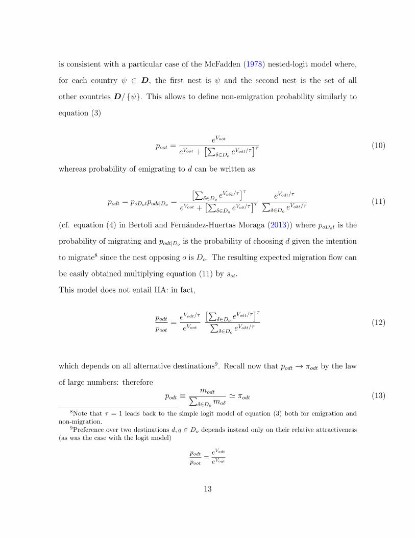
is consistent with a particular case of the McFadden (1978) nested-logit model where,

for each country ψ ∈ D, the first nest is ψ and the second nest is the set of all

other countries D/ ψ. This allows to define non-emigration probability similarly to

equation (3)

poot =eVoot

eVoot +[∑

δ∈Do eVoδt/τ

]τ (10)

whereas probability of emigrating to d can be written as

podt = poDotpodt|Do =

[∑δ∈Do e

Voδt/τ]τ

eVoot +[∑

δ∈Do eVoδ/τ

]τ eVodt/τ∑δ∈Do e

Voδt/τ(11)

(cf. equation (4) in Bertoli and Fernández-Huertas Moraga (2013)) where poDot is the

probability of migrating and podt|Do is the probability of choosing d given the intention

to migrate8 since the nest opposing o is Do. The resulting expected migration flow can

be easily obtained multiplying equation (11) by sot.

This model does not entail IIA: in fact,

podtpoot

=eVodt/τ

eVoot

[∑δ∈Do e

Voδt/τ]τ∑

δ∈Do eVoδt/τ

(12)

which depends on all alternative destinations9. Recall now that podt → πodt by the law

of large numbers: therefore

podt ≡modt∑δ∈Domoδ

' πodt (13)

8Note that τ = 1 leads back to the simple logit model of equation (3) both for emigration andnon-migration.

9Preference over two destinations d, q ∈ Do depends instead only on their relative attractiveness(as was the case with the logit model)

podtpoot

=eVodt

eVoqt

13

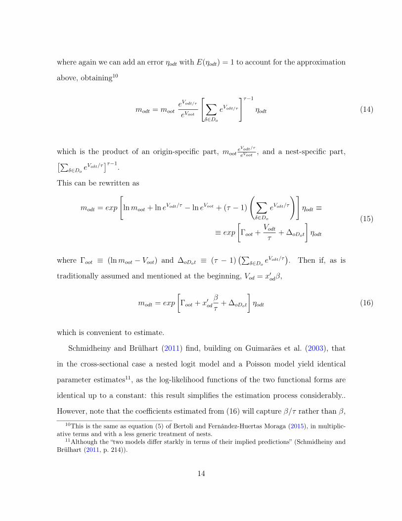
where again we can add an error ηodt with E(ηodt) = 1 to account for the approximation

above, obtaining10

modt = mooteVodt/τ

eVoot

[∑δ∈Do

eVoδt/τ

]τ−1ηodt (14)

which is the product of an origin-specific part, mooteVodt/τ

eVoot, and a nest-specific part,[∑

δ∈Do eVoδt/τ

]τ−1.This can be rewritten as

modt = exp

[lnmoot + ln eVodt/τ − ln eVoot + (τ − 1)

(∑δ∈Do

eVoδt/τ

)]ηodt ≡

≡ exp

[Γoot +

Vodtτ

+ ∆oDot

]ηodt

(15)

where Γoot ≡ (lnmoot − Voot) and ∆oDot ≡ (τ − 1)(∑

δ∈Do eVoδt/τ

). Then if, as is

traditionally assumed and mentioned at the beginning, Vod = x′odβ,

modt = exp

[Γoot + x′od

β

τ+ ∆oDot

]ηodt (16)

which is convenient to estimate.

Schmidheiny and Brülhart (2011) find, building on Guimarães et al. (2003), that

in the cross-sectional case a nested logit model and a Poisson model yield identical

parameter estimates11, as the log-likelihood functions of the two functional forms are

identical up to a constant: this result simplifies the estimation process considerably..

However, note that the coefficients estimated from (16) will capture β/τ rather than β,10This is the same as equation (5) of Bertoli and Fernández-Huertas Moraga (2015), in multiplic-

ative terms and with a less generic treatment of nests.11Although the “two models differ starkly in terms of their implied predictions” (Schmidheiny and

Brülhart (2011, p. 214)).

14

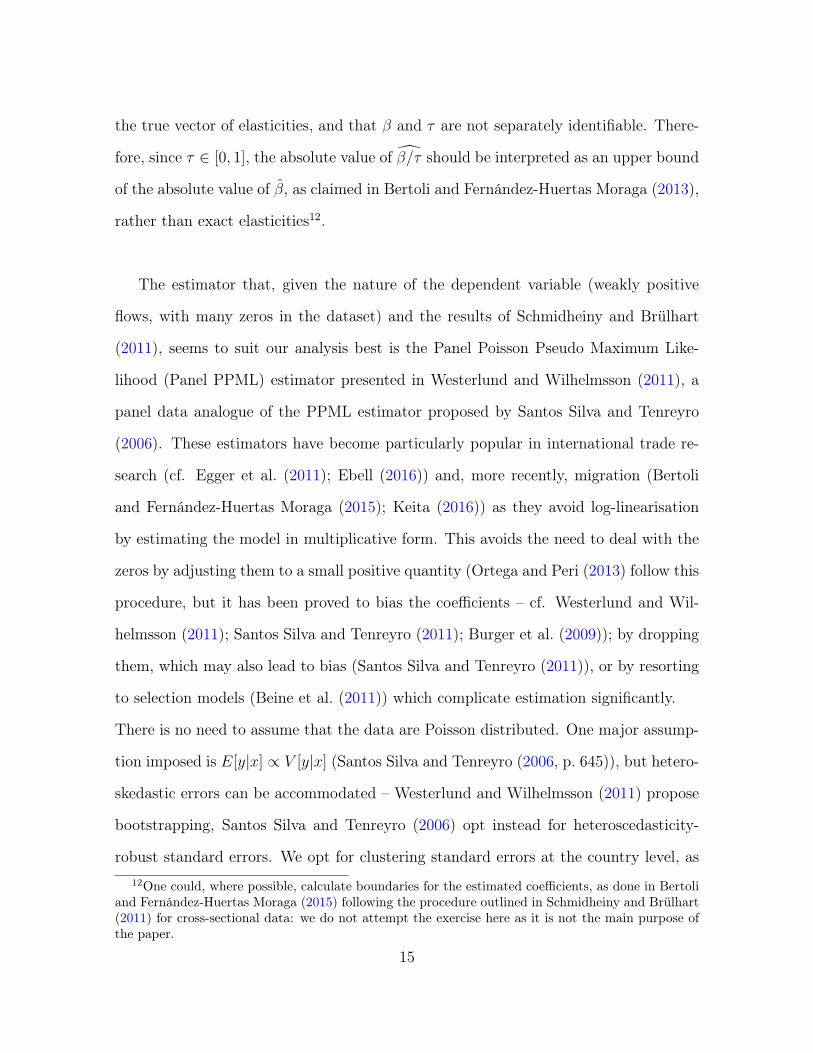
the true vector of elasticities, and that β and τ are not separately identifiable. There-

fore, since τ ∈ [0, 1], the absolute value of β/τ should be interpreted as an upper bound

of the absolute value of β, as claimed in Bertoli and Fernández-Huertas Moraga (2013),

rather than exact elasticities12.

The estimator that, given the nature of the dependent variable (weakly positive

flows, with many zeros in the dataset) and the results of Schmidheiny and Brülhart

(2011), seems to suit our analysis best is the Panel Poisson Pseudo Maximum Like-

lihood (Panel PPML) estimator presented in Westerlund and Wilhelmsson (2011), a

panel data analogue of the PPML estimator proposed by Santos Silva and Tenreyro

(2006). These estimators have become particularly popular in international trade re-

search (cf. Egger et al. (2011); Ebell (2016)) and, more recently, migration (Bertoli

and Fernández-Huertas Moraga (2015); Keita (2016)) as they avoid log-linearisation

by estimating the model in multiplicative form. This avoids the need to deal with the

zeros by adjusting them to a small positive quantity (Ortega and Peri (2013) follow this

procedure, but it has been proved to bias the coefficients – cf. Westerlund and Wil-

helmsson (2011); Santos Silva and Tenreyro (2011); Burger et al. (2009)); by dropping

them, which may also lead to bias (Santos Silva and Tenreyro (2011)), or by resorting

to selection models (Beine et al. (2011)) which complicate estimation significantly.

There is no need to assume that the data are Poisson distributed. One major assump-

tion imposed is E[y|x] ∝ V [y|x] (Santos Silva and Tenreyro (2006, p. 645)), but hetero-

skedastic errors can be accommodated – Westerlund and Wilhelmsson (2011) propose

bootstrapping, Santos Silva and Tenreyro (2006) opt instead for heteroscedasticity-

robust standard errors. We opt for clustering standard errors at the country level, as12One could, where possible, calculate boundaries for the estimated coefficients, as done in Bertoli

and Fernández-Huertas Moraga (2015) following the procedure outlined in Schmidheiny and Brülhart(2011) for cross-sectional data: we do not attempt the exercise here as it is not the main purpose ofthe paper.

15

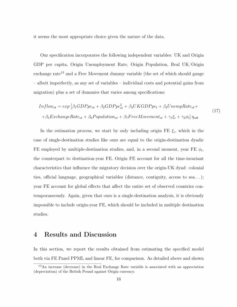
it seems the most appropriate choice given the nature of the data.

Our specification incorporates the following independent variables: UK and Origin

GDP per capita, Origin Unemployment Rate, Origin Population, Real UK/Origin

exchange rate13 and a Free Movement dummy variable (the set of which should gauge

– albeit imperfectly, as any set of variables – individual costs and potential gains from

migration) plus a set of dummies that varies among specifications:

Inflowot = exp[β1GDPpcot + β2GDPpc

2ot + β3UKGDPpct + β4UnempRateot+

+β5ExchangeRateot + β6Populationot + β7FreeMovementot + γ1ξi + γ2φt] ηodt

(17)

In the estimation process, we start by only including origin FE ξi, which in the

case of single-destination studies like ours are equal to the origin-destination dyadic

FE employed by multiple-destination studies, and, in a second moment, year FE φt,

the counterpart to destination-year FE. Origin FE account for all the time-invariant

characteristics that influence the migratory decision over the origin-UK dyad: colonial

ties, official language, geographical variables (distance, contiguity, access to sea. . . );

year FE account for global effects that affect the entire set of observed countries con-

temporaneously. Again, given that ours is a single-destination analysis, it is obviously

impossible to include origin-year FE, which should be included in multiple destination

studies.

4 Results and Discussion

In this section, we report the results obtained from estimating the specified model

both via FE Panel PPML and linear FE, for comparison. As detailed above and shown13An increase (decrease) in the Real Exchange Rate variable is associated with an appreciation

(depreciation) of the British Pound against Origin currency.

16

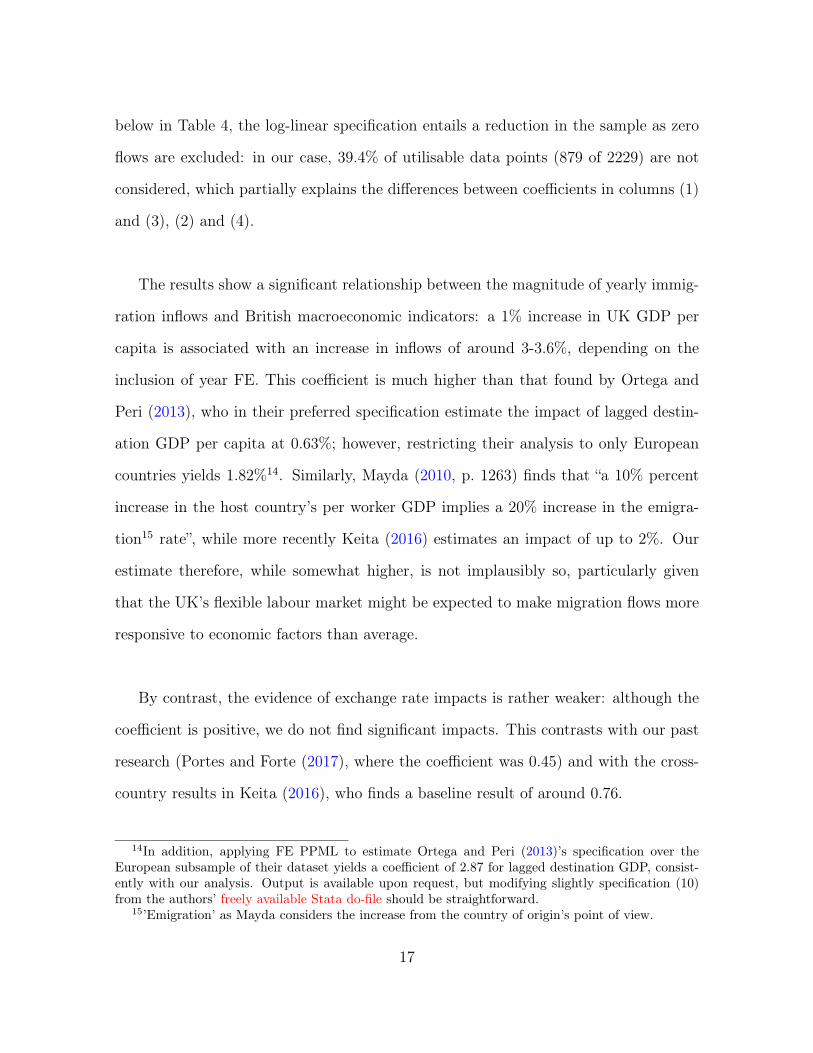
below in Table 4, the log-linear specification entails a reduction in the sample as zero

flows are excluded: in our case, 39.4% of utilisable data points (879 of 2229) are not

considered, which partially explains the differences between coefficients in columns (1)

and (3), (2) and (4).

The results show a significant relationship between the magnitude of yearly immig-

ration inflows and British macroeconomic indicators: a 1% increase in UK GDP per

capita is associated with an increase in inflows of around 3-3.6%, depending on the

inclusion of year FE. This coefficient is much higher than that found by Ortega and

Peri (2013), who in their preferred specification estimate the impact of lagged destin-

ation GDP per capita at 0.63%; however, restricting their analysis to only European

countries yields 1.82%14. Similarly, Mayda (2010, p. 1263) finds that “a 10% percent

increase in the host country’s per worker GDP implies a 20% increase in the emigra-

tion15 rate”, while more recently Keita (2016) estimates an impact of up to 2%. Our

estimate therefore, while somewhat higher, is not implausibly so, particularly given

that the UK’s flexible labour market might be expected to make migration flows more

responsive to economic factors than average.

By contrast, the evidence of exchange rate impacts is rather weaker: although the

coefficient is positive, we do not find significant impacts. This contrasts with our past

research (Portes and Forte (2017), where the coefficient was 0.45) and with the cross-

country results in Keita (2016), who finds a baseline result of around 0.76.

14In addition, applying FE PPML to estimate Ortega and Peri (2013)’s specification over theEuropean subsample of their dataset yields a coefficient of 2.87 for lagged destination GDP, consist-ently with our analysis. Output is available upon request, but modifying slightly specification (10)from the authors’ freely available Stata do-file should be straightforward.

15’Emigration’ as Mayda considers the increase from the country of origin’s point of view.

17

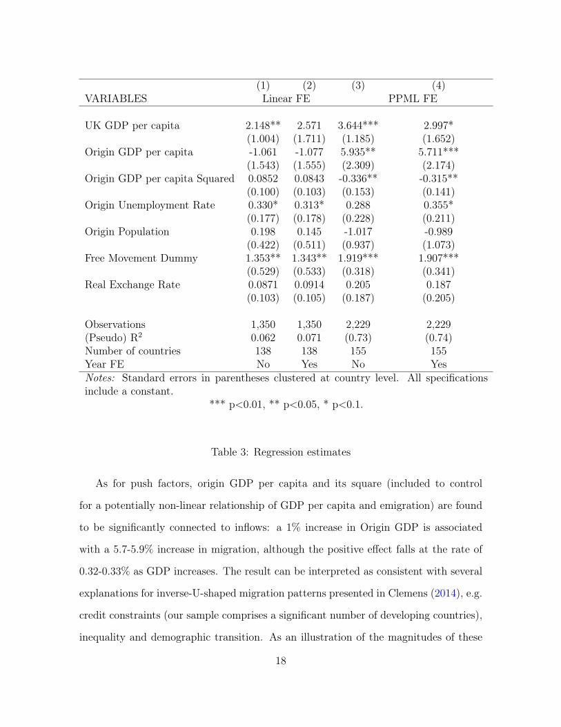
(1) (2) (3) (4)VARIABLES Linear FE PPML FE

UK GDP per capita 2.148** 2.571 3.644*** 2.997*(1.004) (1.711) (1.185) (1.652)

Origin GDP per capita -1.061 -1.077 5.935** 5.711***(1.543) (1.555) (2.309) (2.174)

Origin GDP per capita Squared 0.0852 0.0843 -0.336** -0.315**(0.100) (0.103) (0.153) (0.141)

Origin Unemployment Rate 0.330* 0.313* 0.288 0.355*(0.177) (0.178) (0.228) (0.211)

Origin Population 0.198 0.145 -1.017 -0.989(0.422) (0.511) (0.937) (1.073)

Free Movement Dummy 1.353** 1.343** 1.919*** 1.907***(0.529) (0.533) (0.318) (0.341)

Real Exchange Rate 0.0871 0.0914 0.205 0.187(0.103) (0.105) (0.187) (0.205)

Observations 1,350 1,350 2,229 2,229(Pseudo) R2 0.062 0.071 (0.73) (0.74)Number of countries 138 138 155 155Year FE No Yes No YesNotes: Standard errors in parentheses clustered at country level. All specificationsinclude a constant.

*** p<0.01, ** p<0.05, * p<0.1.

Table 3: Regression estimates

As for push factors, origin GDP per capita and its square (included to control

for a potentially non-linear relationship of GDP per capita and emigration) are found

to be significantly connected to inflows: a 1% increase in Origin GDP is associated

with a 5.7-5.9% increase in migration, although the positive effect falls at the rate of

0.32-0.33% as GDP increases. The result can be interpreted as consistent with several

explanations for inverse-U-shaped migration patterns presented in Clemens (2014), e.g.

credit constraints (our sample comprises a significant number of developing countries),

inequality and demographic transition. As an illustration of the magnitudes of these

18

impacts, the coefficients of GDPpcorigin and GDPpc2origin in column (4) imply that,

for the year 2008, an increase inGDPpc from Indian levels ($1157) to Romanian levels

($8873) would be associated with a 257.6% increase in immigration to the UK from that

country; conversely, an increase from Romanian GDPpc to French GDPpc ($41548)

would be associated with a fall in immigration of around 54%. Fluctuations in unem-

ployment in the source country also appear to have an (albeit less defined) impact on

the decision to migrate, suggesting any impact of origin country economic conditions

appears both through the labour market and wider macroeconomic conditions. Our

estimate implies that a 1% increase in the unemployment rate in the home country

reflects into an increase in immigration of around 0.35%, although the impact is only

significant at the 10% level.

Perhaps the most important and interesting result is that the coefficient associated

with Free Movement that emerges from the analysis of IPS data is almost identical to

that found in Portes and Forte (2017), despite the considerable differences between the

IPS and NINo data, as detailed in Annex A. The existence of free movement between

the UK and a source country is associated with a rise in immigration flows from that

country to the UK of between 570-580%16; this compares to a range of 483-489% found

in our analysis of NINo data. This suggests that, while the two series are very differ-

ent, they are both capturing a very large and consistent positive impact on measured

migration flows from free movement.

As we noted before, the impact of free movement on immigration flows is much

higher than the impact of trade liberalisation (tariff reductions or membership of a16This is calculated as Percentage Change = 100 [exp(β7)− 1]; the usual approximation centred

around ln(1+ε) ' 1+ε is only valid for very small ε and starts failing quite significantly for coefficientshigher than 0.1.

19

free trade area) on trade volumes found in the trade literature, reflecting the fact that

“absent free movement, barriers to labour mobility between countries are much higher

than trade barriers” (Portes and Forte (2017, p. S33)). Although we do not present

forecasts in this paper, our analysis here reaffirms and strengthens our earlier conclusion

that free movement led to a large rise in migration flows from other EU countries to

the UK; Brexit, and the associated end of free movement, is therefore likely to lead to

a very substantial reduction in such flows.

For the reasons set out in Portes (2016), this is likely to be the case even if the UK

adopts a relatively liberal approach to some categories of EU migrants (either by skill

level or by sector); and is likely to affect medium and high skilled migration as well

as low-skilled or low-paid migration. The negative economic consequences for the UK

could be large.

5 Improving immigration statistics

We are encouraged by the fact that our analysis of IPS data are consistent with both

theory and our previous work using National Insurance number data. However, this

does not negate the broader point that improvements to UK immigration data are

long overdue. Greater international mobility, particularly short-term migration of un-

certain duration, means that survey responses are inherently likely to be inaccurate;

this compounds the already existing problem that any sample survey based on pas-

sengers will only pick up a relatively small number of immigrants and emigrants, since

most passengers are tourists or business visitors. Hence, while the IPS gives a reas-

onably reliable assessment of the overall balance between high-level immigration and

emigration, granular analysis is very difficult. If the Government still stands by its aim

of reducing net immigration to the tens of thousands, it might prefer doing so using a

20

source that does not have a standard error in the order of the tens of thousands.

Alternative sources of migration flows (APS, NINo registrations) have been used

to support the findings of the IPS and maintain its credibility through changes and

revisions, but the rising availability of administrative data presents a great opportunity

for a shift in their importance. The ONS (Office for National Statistics (2016a)) has

attempted to reconcile administrative data with the IPS data (although not with the

APS), using data from the HMRC and the Department for Work and Pensions (DWP),

linked via National Insurance Numbers; but so far this was a one-off exercise and has

not fed into ongoing work. While previously access to large administrative datasets was

difficult for both legal and practical reasons, advances in technology and the passage

of the Digital Economy Bill mean that such barriers are much less of a constraint. As

the UK Statistics Authority puts it (UK Statistics Authority (2017)):

There are a range of migration-related datasets available across different

Government departments, including those from HMRC, DWP, ONS and

the Home Office. The key to a comprehensive picture lies in bringing these

datasets together.

Equally important is enabling access to administrative data for independent external

analysis. There is huge academic as well as policy interest in immigration; however,

research is heavily constrained – as this paper and our earlier one show – by the lack

of reliable, detailed disaggregated data. Enabling such access would benefit policy,

research and the UK’s highly charged immigration debate.

21

6 Conclusion

This paper contributes to the British debate on immigration by presenting evidence

on the factors that shape migratory inflows to the UK. It is akin to Portes and Forte

(2017) in this purpose, but it expands the state of knowledge by making use of flows

based on the International Passenger Survey rather than on National Insurance Regis-

trations, thus directly shedding light on the comparability (or lack thereof) of the two

sources.

First, our brief analysis of the IPS methodology and history puts on display the

major weakness of the survey, which has been highlighted in the policy debate: a small

sample, which causes large statistical uncertainty and is ill-suited to capture increas-

ingly more complex migration patterns. Since the LTIM (of which the IPS is a principal

component) nevertheless remains the official source for migration statistics, we analyse

the impact of both macroeconomic indicators and policy variables on migration using

a theoretically-consistent Poisson estimator.

The results are in line with theory and the existing literature: we find large impacts

of push (Origin GDP) and pull (UK GDP) factors, and tentative evidence of the impact

of Origin unemployment rate fluctuations. The large (compared to multiple-destination

analyses) impacts associated with some of the drivers may reflect the flexibility of the

UK labour markets. Interestingly, the six-fold increase in IPS inflows associated with

switching to Free Movement is quantitatively similar to the increase in NINos we found

in earlier research, suggesting our earlier conclusion that ending free movement will res-

ult in a substantial fall in migration is robust to the use of different data sources.

22

References

Anderson, James E and Eric Van Wincoop (2003). “Gravity with gravitas: a solution

to the border puzzle”. The American Economic Review 93.1, pp. 170–192.

Beine, Michel, Simone Bertoli and Jesús Fernández-Huertas Moraga (2015). “A prac-

titioners’ guide to gravity models of international migration”. The World Economy

39.4, pp. 496–512.

Beine, Michel, Pauline Bourgeon and Jean-Charles Bricogne (2013). “Aggregate fluc-

tuations and international migration”. CESifo Working Paper No.4379.

Beine, Michel, Frédéric Docquier and Çağlar Özden (2011). “Diasporas”. Journal of

Development Economics 95.1, pp. 30–41.

Bertoli, Simone and Jesús Fernández-Huertas Moraga (2013). “Multilateral resistance

to migration”. Journal of Development Economics 102, pp. 79–100.

— (2015). “The size of the cliff at the border”. Regional Science and Urban Economics

51, pp. 1–6.

Burger, Martijn, Frank Van Oort and Gert-Jan Linders (2009). “On the specification of

the gravity model of trade: zeros, excess zeros and zero-inflated estimation”. Spatial

Economic Analysis 4.2, pp. 167–190.

Chudik, Alexander and M Hashem Pesaran (2015). “Common correlated effects es-

timation of heterogeneous dynamic panel data models with weakly exogenous re-

gressors”. Journal of Econometrics 188.2, pp. 393–420.

Clemens, Michael A (2014). “Does development reduce migration?” International Hand-

book on Migration and Economic Development, pp. 152–185.

Ebell, Monique (2016). “Assessing the impact of trade agreements on trade”. National

Institute Economic Review 238.1, R31–R42.

23

Egger, Peter et al. (2011). “The trade effects of endogenous preferential trade agree-

ments”. American Economic Journal: Economic Policy 3.3, pp. 113–143.

European Union Committee (2017). Brexit: UK-EU movement of people. 14th Report

of Session 2016-17. url: goo.gl/Qk0L1S (visited on 07/03/2017).

Feenstra, Robert C, Robert Inklaar and Marcel P Timmer (2015). “The Next Genera-

tion of the Penn World Table”. American Economic Review 105.10, pp. 3150–3182.

url: ggdc.net/pwt.

Grogger, Jeffrey and Gordon H Hanson (2011). “Income maximization and the selection

and sorting of international migrants”. Journal of Development Economics 95.1,

pp. 42–57.

Guimarães, Paulo, Octávio Figueirdo and Douglas Woodward (2003). “A tractable

approach to the firm location decision problem”. The Review of Economics and

Statistics 85.1, pp. 201–204.

House of Commons (2013). Migration Statistics. Seventh Report of Session 2013-14.

url: goo.gl/VFlTc9 (visited on 07/03/2017).

Keita, Sekou (2016). “Bilateral real exchange rates and migration”. Applied Economics

48.31, pp. 2937–2951.

Mayda, Anna Maria (2010). “International migration: A panel data analysis of the

determinants of bilateral flows”. Journal of Population Economics 23.4, pp. 1249–

1274.

McFadden, Daniel (1974). “Conditional logit analysis of qualitative choice behavior”.

In: Frontiers in Econometrics. Ed. by P. Zarembka. New York: Academic Press,

pp. 105–142.

— (1978). “Modelling the choice of residential location”. In: Spatial Interaction: The-

ories and Models. Ed. by A. Karlgvist et al. Amsterdam: North Holland, pp. 75–

96.

24

Migration Watch (2016). UK immigration policy outside the EU. url: goo.gl/N3s5iE

(visited on 07/03/2017).

Office for National Statistics (2014). Quality of Long-Term International Migration

Estimates from 2001 to 2011. url: goo.gl/wsccqn (visited on 07/03/2017).

— (2015a). Long-Term International Migration Estimates - Methodology Document.

url: goo.gl/Na8qe5 (visited on 07/03/2017).

— (2015b). Travel Trends. url: goo.gl/VNWMQE (visited on 07/03/2017).

— (2016a). Comparing sources of international statistics: December 2016. url: goo.

gl/qHY30y (visited on 07/03/2017).

— (2016b). International Passenger Survey 4.06, country of birth by citizenship. url:

goo.gl/je6igU (visited on 07/03/2017).

— (2016c). Note on the difference between National Insurance number registrations

and the estimate of long-term international migration: 2016. url: goo.gl/6BSIOo

(visited on 07/03/2017).

— (2016d). Travel trends: 2015. url: goo.gl/wk6aut (visited on 07/03/2017).

— (2017). Long-Term International Migration - Quality and Methodology Information.

url: goo.gl/TrFSyw (visited on 07/03/2017).

Ortega, Francesc and Giovanni Peri (2013). “The effect of income and immigration

policies on international migration”. Migration Studies 1.1, pp. 47–74.

Portes, Jonathan (2016). “Immigration after Brexit”. National Institute Economic Re-

view 238.1, R13–R21.

Portes, Jonathan and Giuseppe Forte (2017). “The economic impact of Brexit-induced

reductions in migration”. Oxford Review of Economic Policy 33.S1, S31–S44.

Santos Silva, João and Silvana Tenreyro (2006). “The log of gravity”. The Review of

Economics and statistics 88.4, pp. 641–658.

25

Santos Silva, João and Silvana Tenreyro (2010). “On the existence of the maximum

likelihood estimates in Poisson regression”. Economics Letters 107.2, pp. 310–312.

— (2011). “Further simulation evidence on the performance of the Poisson pseudo-

maximum likelihood estimator”. Economics Letters 112.2, pp. 220–222.

Schmidheiny, Kurt and Marius Brülhart (2011). “On the equivalence of location choice

models: Conditional logit, nested logit and Poisson”. Journal of Urban Economics

69.2, pp. 214–222.

UK Statistics Authority (2013a). Review of the Robustness of the International Pas-

senger Survey. url: goo.gl/QoBfD3 (visited on 07/03/2017).

— (2013b). UK Statistics Authority response to Migration Statistics. url: goo . gl /

sCV5B3 (visited on 07/03/2017).

— (2016). Differences between DWP statistics on National Insurance Numbers alloc-

ated to adult overseas nationals and ONS migration figures. url: goo.gl/obvjbi

(visited on 07/03/2017).

— (2017). Migration Statistics. url: goo.gl/F9urbi (visited on 07/03/2017).

Westerlund, Joakim and Fredrik Wilhelmsson (2011). “Estimating the gravity model

without gravity using panel data”. Applied Economics 43.6, pp. 641–649.

World Bank (2017). World Development Indicators. url: data.worldbank.org/data-

catalog/world-development-indicators (visited on 07/03/2017).

26

Annexes

A National Insurance Registrations and IPS: a Comparison

Since we made use of National Insurance Number registrations17 in previous research as

a measure of high-frequency migration flows, it is sensible to focus on the similarities

and differences this source presents with IPS. Registering for a NINo is voluntary;

however, it is necessary for any non-British citizen who wishes to regularly work or

claim benefits. As set out in our earlier paper, there a number of reasons why migrant

flows as measured using NINos will differ from inflows in the IPS:

• Sampling and other errors in the IPS, as noted in Section 2;

• NINo registrants who are not long-term migrants for the purposes of the IPS

(that is, they do not intend to stay for more than 12 months);

• Immigrants recorded in the IPS who do not register for a NINO (because they do

not intend to work or claim benefits, or they work solely in the “black economy”)

In addition, there is no obligation to report leaving the country or to deregister with

DWP or HMRC; it is thus impossible to know how many of those migrants who have

registered for a NINos subsequently left the country (and if so when). However, lon-

gitudinal administrative data held by DWP and HMRC (on tax and NI contributions

and benefits claimed) could in principle provide considerable information on this.

Notwithstanding those differences, NINo registrations and IPS inflows appear to

move together: the correlation coefficient between origin-year NINo registrations and

IPS inflows for the broader dataset (i.e. not limited to the estimation sample) is 0.76,17By NINo registrations we refer to the stock of released NINos divided by country of worker

provenance and quarter of release. These figures are available through Stat-Xplore, the online gatewayto DWP’s publicly accessible statistics.

27

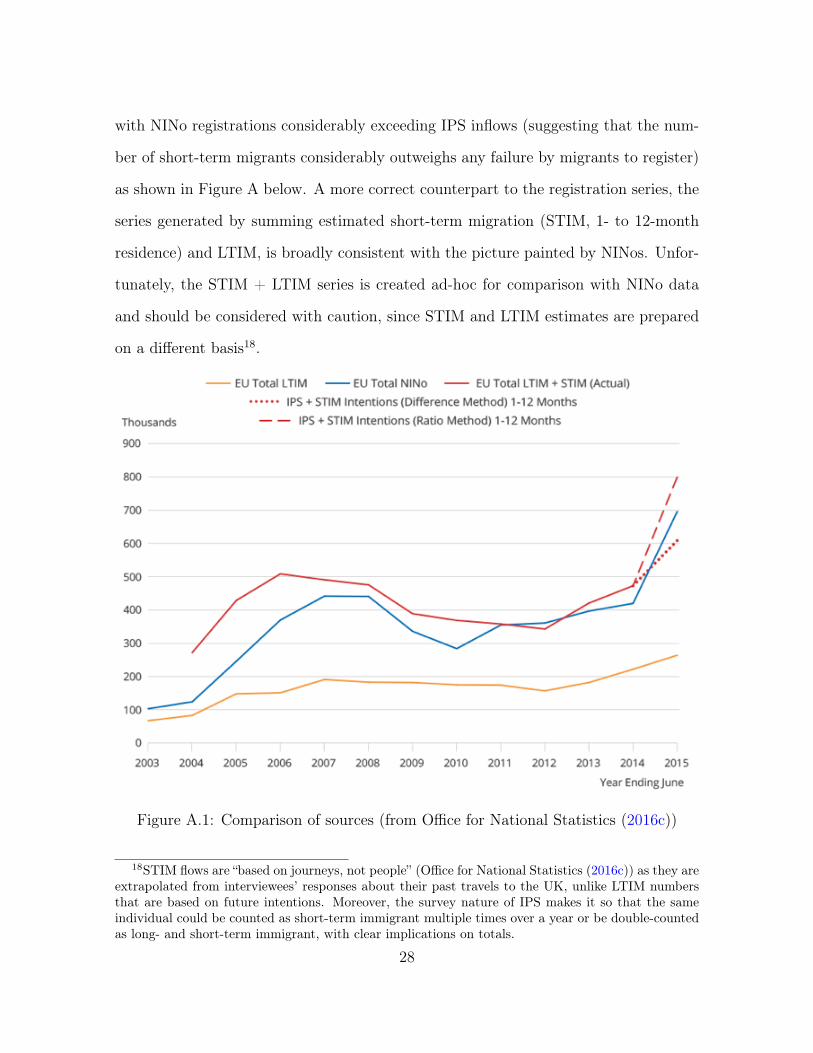
with NINo registrations considerably exceeding IPS inflows (suggesting that the num-

ber of short-term migrants considerably outweighs any failure by migrants to register)

as shown in Figure A below. A more correct counterpart to the registration series, the

series generated by summing estimated short-term migration (STIM, 1- to 12-month

residence) and LTIM, is broadly consistent with the picture painted by NINos. Unfor-

tunately, the STIM + LTIM series is created ad-hoc for comparison with NINo data

and should be considered with caution, since STIM and LTIM estimates are prepared

on a different basis18.

Figure A.1: Comparison of sources (from Office for National Statistics (2016c))

18STIM flows are “based on journeys, not people” (Office for National Statistics (2016c)) as they areextrapolated from interviewees’ responses about their past travels to the UK, unlike LTIM numbersthat are based on future intentions. Moreover, the survey nature of IPS makes it so that the sameindividual could be counted as short-term immigrant multiple times over a year or be double-countedas long- and short-term immigrant, with clear implications on totals.

28

The aforementioned issues do not take away from some clear advantages of quan-

tifying immigration using NINos: first, there is negligible (if at all) uncertainty about

the number of registrations that the DWP makes, as all records come from a unique

administrative source; second, applying for a NINo requires booking an appointment,

showing up at an assigned JobCentre Plus and potentially waiting weeks to obtain the

code, so it does not seem unfair to assume that it is a better indicator of immigration

than an intention-based discretionary survey upon arrival. As we discuss in Section

5, we believe NINo registrations are a thorough base that can be supplemented with

more administrative information to obtain a superior and more faceted source for both

short- and long-term immigration statistics.

B List of countries analysed

The IPS publishes yearly inflows and outflows (measured in thousands passengers) for

240 entities (countries and territories overseas). The WDI and Penn Tables only include

the information necessary to our analysis for a wide but limited sample of countries.

The countries included in the estimation sample are the following:

• Albania

• Algeria

• Angola

• Argentina

• Armenia

• Australia

• Austria

• Bahamas

• Bahrain

• Bangladesh

• Barbados

• Belgium

• Belize

• Benin

• Bhutan

• Bolivia

• Bosnia andHerzegovina

• Botswana

• Brazil

• Brunei

• Bulgaria

• Burkina

• Burma

• Burundi

• Cambodia

• Cameroon

• Canada

• Cape Verde

• CentralAfrican Re-public

• Chad

• Chile

• China

• Colombia

• Comoros

• Congo29

• D R of Congo

• Costarica

• Croatia

• Cyprus

• Czech Repub-lic

• Denmark

• DominicanRepublic

• Ecuador

• Egypt

• El Salvador

• EquatorialGuinea

• Estonia

• Ethiopia

• Fiji

• Finland

• France

• Gabon

• Gambia

• Georgia

• Germany

• Ghana

• Greece

• Guatemala

• Guinea

• Guinea Bissau

• Haiti

• Honduras

• Hong Kong

• Hungary

• Iceland

• India

• Indonesia

• Iran

• Iraq

• Ireland

• Israel

• Italy

• Ivory Coast

• Jamaica

• Japan

• Jordan

• Kazakhstan

• Kenya

• Kuwait

• Kyrgyzstan

• Laos

• Latvia

• Lebanon

• Lesotho

• Liberia

• Lithuania

• Luxembourg

• Macao

• Macedonia

• Madagascar

• Malawi

• Malaysia

• Maldives

• Mali

• Malta

• Mauritania

• Mauritius

• Mexico

• Moldova

• Mongolia

• Montenegro

• Morocco

• Mozambique

• Namibia

• Nepal

• Netherlands

• New Zealand

• Nicaragua

• Niger

• Nigeria

• Norway

• Oman

• Pakistan

• Panama

• Paraguay

• Peru

• Philippines

• Poland

• Portugal

• Qatar

• Romania

• Russia

• Rwanda

• Saudi Arabia

• Senegal

• Sierra Leone

• Singapore

• Slovakia

• Slovenia

• South Africa

• South Korea

• Spain

• Sri Lanka

• Sudan

• Suriname

• Swaziland

• Sweden

• Switzerland

• Tanzania30

• Thailand

• Togo

• Trinidad andTobago

• Tunisia

• Turkey

• Uganda

• Ukraine

• United ArabEmirates

• United States

• Uruguay

• Venezuela

• Vietnam

• Yemen

• Yugoslavia

• Zambia

• Zimbabwe

31