Visual-Hull Reconstructionfrom Uncalibrated and Unsynchronized Video Streams

Sudipta N. Sinha and Marc Pollefeys{ssinha,marc}@cs.unc.eduDepartment of Computer Science

University of North Carolina at Chapel Hill, USA.

Abstract

We present an approach for automatic reconstruction of adynamic event using multiple video cameras recording fromdifferent viewpoints. Those cameras do not need to be cal-ibrated or even synchronized. Our approach recovers allthe necessary information by analyzing the motion of thesilhouettes in the multiple video streams. The first stepconsists of computing the calibration and synchronizationfor pairs of cameras. We compute the temporal offset andepipolar geometry using an efficient RANSAC-based algo-rithm to search for the epipoles as well as for robustness.In the next stage the calibration and synchronization forthe complete camera network is recovered and then refinedthrough maximum likelihood estimation. Finally, a visual-hull algorithm is used to the recover the dynamic shape ofthe observed object. For unsynchronized video streams sil-houettes are interpolated to deal with subframe temporaloffsets. We demonstrate the validity of our approach byobtaining the calibration, synchronization and 3D recon-struction of a moving person from a set of 4 minute videosrecorded from 4 widely separated video cameras.

1. IntroductionIn surveillance camera networks, live video of a dynamicscene is often captured from multiple views. We aim to au-tomatically recover the 3D reconstruction of the dynamicevent, as well as the calibration and synchronization, usingonly the input videos. Different pairs of archived video se-quences may have a time-shift between them since record-ing would be triggered by moving objects, with differentcameras being activated at different instants in time. Ourmethod simultaneously recovers the synchronization andepipolar geometry of such a camera pair. This method isparticularly useful for shape-from-silhouette systems [3, 4,14] as visual-hulls can now be reconstructed from uncali-brated and unsynchronized video of moving objects.

Different existing structure-from-motion approaches us-ing silhouettes [21, 20, 22] either require good initializationor only work for certain camera configurations and most of

Figure 1: Synchronization, calibration and 3D visual-hullreconstruction from 4 video streams.

them require static scenes. Traditionally, calibration objectslike checkerboard patterns or LED’s have been used for cal-ibrating multi-camera systems [23] but this requires physi-cal access to the observed space. This is often impracticaland costly for surveillance applications and could be impos-sible for remote camera networks or networks deployed inhazardous environments. Our method can calibrate or recal-ibrate such cameras remotely and also handle wide-baselinecamera pairs, arbitrary camera configurations and a lack ofphotometric calibration.

At the core of our approach is a robust RANSAC [5]based algorithm that computes the epipolar geometry fromtwo video sequences of dynamic objects. This algorithmis based on the constraints arising from the correspondenceof frontier points and epipolar tangents [21, 13, 2] of sil-houettes in two views. These are points on an objects’ sur-face which project to points on the silhouette in two views.Epipolar lines passing through the images of a frontier pointmust correspond. Such epipolar lines are also tangent tothe silhouettes at the imaged frontier points. Previous workused those constraints to refine an existing epipolar geom-etry [13, 2]. Here we take advantage of the fact that videosequences of dynamic objects will contain many differentsilhouettes, yielding many constraints that must be satis-

����

����

��������

����������������

������

������

���

���

������

������

���

���

������

������

������

������

������

������ e 12

21e

1 2l lview 1

Π

C

C2

1

X

Yview 2

S S1 2

Figure 2: (a)Frontier Points and Epipolar Tangents.(b) TheTangent Envelope.

fied. We use RANSAC [5] not only to remove outliers insilhouette data but also to sample the space of unknown pa-rameters. We first demonstrate how the method works withsynchronized video. We then describe how pair-wise funda-mental matrices and frontier point can be used to compute aprojective reconstruction of the complete camera network,which is then refined to a metric reconstruction. An exten-sion of the RANSAC based algorithm allows us to recoverthe temporal offset between pairs of unsynchronized videosequences acquired at the same frame rate. A method tosynchronize the whole camera network is then presented.Finally, the deforming shape is reconstructed using a shape-from-silhouette approach taking subframe temporal offsetsinto account through interpolation.

In Sec. 2 we present the background theory. Sec. 3 de-scribes the algorithm that computes the epipolar geometryfrom dynamic silhouettes. Full camera network calibrationis discussed in Sec. 4 while Sec. 5 describes how we dealwith unsynchronized video. Section 6 described our recon-struction approach. Experimental results are presented indifferent sections of the paper and we conclude with scopefor future work in Sec. 7.

2. Background and Previous WorkOur algorithm exploits the constraints arising from the cor-respondence of frontier points and epipolar tangents [21,13]. Frontier points on an objects’ surface are 3D pointswhich project to points on the silhouette in the two views.In Fig. 2(a), X and Y are frontier points on the apparentcontours C1 and C2, which project to points on the silhou-ettes S1 and S2 respectively. The projection of Π, the epipo-lar plane tangent to X gives rise to corresponding epipolarlines l1 and l2 which are tangent to S1 and S2 at the imagesof X in the two images respectively. No other point on S1

and S2 other than the images of frontier points, X and Ycorrespond. Morever, the image of the frontier points cor-responding to the outer-most epipolar tangents [21] mustlie on the convex hull of the silhouette. The silhouettes arestored in a compact data structure called the tangent enve-lope, [16] (see Fig. 2(b)). We only need of the order of 500

Figure 3: (a) The 4D hypothesis of the epipoles (not in pic-ture). (b) All frontier points for a specific hypothesis and apair of transferred epipolar lines l1, l2.

bytes per frame.Video of dynamic objects contain many different silhou-ettes, yielding many constraints that are satisfied by the trueepipolar geometry. Unlike other algorithms, e.g. [6], whosearch for all possible frontier points and epipolar tangentson a single silhouette, we only search for the outermostfrontier points and epipolar tangents, but for many silhou-ettes. Only using the outermost epipolar tangents allowsus to be far more efficient because the data structures aresimpler and there are no self-occlusions. Sufficient motionof the object within the 3D observed space gives rise to agood spatial distribution of frontier points and increases theaccuracy of the fundamental matrix.

3. Computing the Epipolar Geometry

Computing the epipolar geometry from silhouettes is notas simple as computing it from points. The reason is thathaving two corresponding silhouettes doesn’t immediatelyyield usable equations. We first need to know where thefrontier points are and this is dependent on the epipolar ge-ometry. This is thus a typical “chicken and egg” problem.

However, this is not as bad as it seems. We do not need thefull epipolar geometry. The location of the epipoles (4 outof 7 parameters) is sufficient to determine the epipolar tan-gents and the frontier points. Our approach will thus consistof randomly generating epipole hypotheses and then verifythat the bundle of epipolar tangents to all the silhouettes areconsistent. One of the key elements to the success of our al-gorithm is to have a very efficient data representation and togenerate a proper distribution of epipoles in our samplingprocess. This approach is explained more in detail in theremainder of this section.

The RANSAC-based algorithm takes two sequences asinput, where the j th frame in sequence i is denoted by S j

i

and the corresponding tangent envelope by T (S ji ). Fij is

the fundamental matrix between view i and view j, (trans-fers points in view i to epipolar lines in view j) and e ij , theepipole in view j of camera center i. While a fundamen-tal matrix has 7 dof ’s, we only randomly sample in a 4Dspace because if the epipoles are known, the frontier pointscan be determined, and the remaining degrees of freedom ofthe epipolar geometry can be derived from them. The pen-cil of epipolar lines in each view centered on the epipoles,is considered as a 1D projective space [7] [ Ch.8, p.227 ].The epipolar line homography between two such 1D pro-jective spaces can be represented by a 2D homography tobe applied to the 2D representation of the lines. Know-ing the epipoles eij , eji and the epipolar line homographyfixes Fij . Three pairs of corresponding epipolar lines aresufficient to determine the epipolar line homography H −�

ij

so that it uniquely determines the transfer of epipolar lines(note that H−�

ij is only determined up to 3 remaining de-grees of freedom, but those do not affect the transfer ofepipolar lines). The fundamental matrix is then uniquelygiven by Fij = [eij ]×Hij .At every iteration, we randomly choose the rth frames fromeach of the two sequences. As shown in Fig. 3(a), we then,randomly sample independent directions l 1

1 from T (Sr1) and

l12 from T (Sr2) for the first pair of tangents in the two views.

We choose a second pair of directions l21 from T (Sr1) and l22

from T (Sr2) such that l2i = l1i − x for i = 1, 2 where x is

drawn from the normal distribution, N(180, σ)1. The inter-sections of the two pair of tangents produces the epipole hy-pothesis (e12 , e21). We next randomly pick another pair offrames q, and compute either the first pair of tangents or thesecond pair. Let us denote this third pair of lines by l 3

1 tan-gent to CH(Sq

1) and l32 tangent to CH(Sq2) (see Fig 3(a)).

Hij is computed from (lki ↔ lkj ; k = 1. . .3)2. The entities(eij ,eji ,Hij) form the model hypothesis for every iteration

1We use σ = 60 in our experiments. In case silhouettes are clipped inthis frame, the second pair of directions is chosen from another frame.

2For simplicity we assume that the first epipolar tangent pair corre-sponds as well as the second pair of tangents. This limitations could beeasily removed by verifying both hypotheses for every random sample.

of our algorithm.Once a model for the epipolar geometry is available, we

verify its accuracy. We do this by computing tangents fromthe hypothesized epipoles to the whole sequence of silhou-ettes in each of the two views. For unclipped silhouetteswe obtain two tangents per frame whereas for clipped sil-houettes, there may be one or even zero tangents. Everytangent in the pencil of the first view is transferred throughH−�

ij to the second view (see Fig. 3(b)) and the reprojec-tion error of the transferred line from the point of tangencyin that particular frame is computed. We count the outliersthat exceed a reprojection error threshold (we choose thisto be 5 pixels) and throw away our hypothesis if the outliercount exceeds a certain fraction of the total expected inliercount. This allows us to abort early whenever the modelhypothesis is completely inaccurate. Thus tangents to allthe silhouettes Sj

i , j ε 1 . . . M in view i, i = 1, 2 wouldbe computed only for a promising hypothesis. For all suchpromising hypotheses an inlier count is maintained using alower threshold (we choose this to be 1.25 pixels).

After a solution with a sufficiently high inlier fractionhas been found, or a preset maximum number of itera-tions has been exhausted, we select the solution with themost inliers and improve our estimate of F for this hypoth-esis through an iterative process of non-linear Levenberg-Marcquardt minimization while continuing to search for ad-ditional inliers. Thus, at every iteration of the minimization,we recompute the pencil of tangents for the whole silhou-ettes sequence Sj

i , j ε 1 . . . M in view i, i = 1, 2 untilthe inlier count converges. The cost function minimized isthe distance between the tangency point and the transferredepipolar line (see Fig. 3(b)) in both images. At this stage wealso recover the frontier point correspondences (the pointsof tangency) for the full sequence of silhouettes in the twoviews. An outline of the algorithm is given in Algorithm 1.

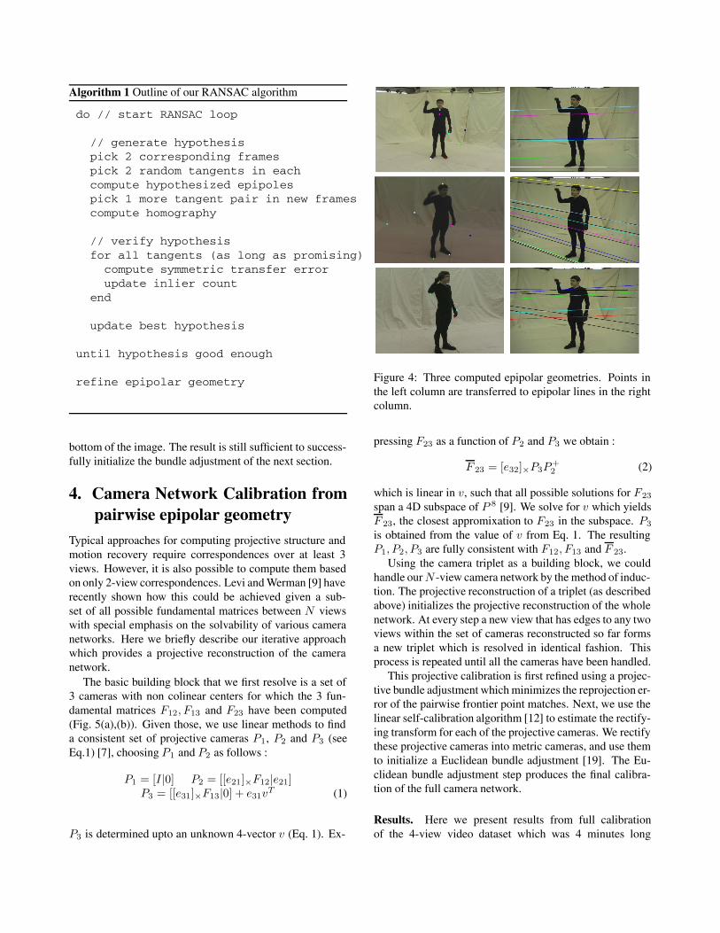
Results. This approach works well in practice and hasbeen demonstrated on multiple datasets recorded by ourselfand by others [16]. Here we show some results obtainedfrom the 4-view dataset that is used throughout this paper.In Figure 4 the computed epipolar geometry F14, F24 andF34 are shown. The black epipolar lines correspond to theinitial epipolar geometry computed as discussed in this sec-tion, the colored epipolar lines correspond to the epipolargeometry once it is made consistent over a triplet of cam-eras3. One can notice the significant improvement for pair2-4 once three-view consistency is enforced. The result forpair 3-4 is less accurate. This is due to clipping of the sil-houette at the feet in most of the frames, therefore onlyyielding a small number of extremal frontier points at the

3Note that the final epipolar geometry is refined even further throughbundle adjustment, see next section

Algorithm 1 Outline of our RANSAC algorithm

do // start RANSAC loop

// generate hypothesispick 2 corresponding framespick 2 random tangents in eachcompute hypothesized epipolespick 1 more tangent pair in new framescompute homography

// verify hypothesisfor all tangents (as long as promising)

compute symmetric transfer errorupdate inlier count

end

update best hypothesis

until hypothesis good enough

refine epipolar geometry

bottom of the image. The result is still sufficient to success-fully initialize the bundle adjustment of the next section.

4. Camera Network Calibration frompairwise epipolar geometry

Typical approaches for computing projective structure andmotion recovery require correspondences over at least 3views. However, it is also possible to compute them basedon only 2-view correspondences. Levi and Werman [9] haverecently shown how this could be achieved given a sub-set of all possible fundamental matrices between N viewswith special emphasis on the solvability of various cameranetworks. Here we briefly describe our iterative approachwhich provides a projective reconstruction of the cameranetwork.

The basic building block that we first resolve is a set of3 cameras with non colinear centers for which the 3 fun-damental matrices F12, F13 and F23 have been computed(Fig. 5(a),(b)). Given those, we use linear methods to finda consistent set of projective cameras P1, P2 and P3 (seeEq.1) [7], choosing P1 and P2 as follows :

P1 = [I|0] P2 = [[e21]×F12|e21]P3 = [[e31]×F13|0] + e31v

T (1)

P3 is determined upto an unknown 4-vector v (Eq. 1). Ex-

Figure 4: Three computed epipolar geometries. Points inthe left column are transferred to epipolar lines in the rightcolumn.

pressing F23 as a function of P2 and P3 we obtain :

F 23 = [e32]×P3P+2 (2)

which is linear in v, such that all possible solutions for F23

span a 4D subspace of P 8 [9]. We solve for v which yieldsF 23, the closest appromixation to F23 in the subspace. P3

is obtained from the value of v from Eq. 1. The resultingP1, P2, P3 are fully consistent with F12, F13 and F 23.

Using the camera triplet as a building block, we couldhandle our N -view camera network by the method of induc-tion. The projective reconstruction of a triplet (as describedabove) initializes the projective reconstruction of the wholenetwork. At every step a new view that has edges to any twoviews within the set of cameras reconstructed so far formsa new triplet which is resolved in identical fashion. Thisprocess is repeated until all the cameras have been handled.

This projective calibration is first refined using a projec-tive bundle adjustment which minimizes the reprojection er-ror of the pairwise frontier point matches. Next, we use thelinear self-calibration algorithm [12] to estimate the rectify-ing transform for each of the projective cameras. We rectifythese projective cameras into metric cameras, and use themto initialize a Euclidean bundle adjustment [19]. The Eu-clidean bundle adjustment step produces the final calibra-tion of the full camera network.

Results. Here we present results from full calibrationof the 4-view video dataset which was 4 minutes long

Figure 5: (a) Three non-degenerate views for which weestimate all F matrices. (b) The three-view case. F 23

is the closest approximation of F23 we compute. (c)&(d)The induction steps used to resolve larger graphs using ourmethod.

Figure 6: Recovered camera configuration and visual-hullreconstruction of person.

and captured at 30 fps [14] (see Fig. 6). We com-puted the projective cameras from the fundamental matri-ces F12, F13, F23, F14, F24. On average, we obtained onecorrect solution, one which converged to a global mini-mum after non-linear refinement for every 5000 hypothe-sis4. This took approximately 15 seconds of computationtime on a 3GHz PC with 1 GB RAM. Assuming a Poissondistribution, 15,000 hypothesis would yield approximately95% probability of finding the correct solution and 50,000hypothesis would yield 99.99% probability.

F23 and F24 had to be adjusted by the method describedin Section 4, which actually improved our initial estimates.The projective camera estimates were then refined through aprojective bundle adjustment (reducing the reprojection er-ror from 4.6 pixels to 0.44 pixels). The final reprojection er-ror after self-calibration and metric bundle adjustment was0.73 pixels.

In typical video, outermost frontier points and epipolartangents often remain stationary over a long time. Such

4For all different camera pairs we get respectively one in 5555, 4412,4168, 3409, 9375 and 5357. The frequency was computed over a total of150,000 hypothesis for each viewpair.

static frames are redundant and representative keyframesmust be chosen to make the algorithm faster. We do thisby considering hypothetical epipoles (at the 4 image cor-ners), pre-computing tangents to all the silhouettes in thewhole video and binning them and picking representativekeyframes such that at least one from each bin is selected.For the 4-view dataset, we ended up with 600-700 out of7500 frames.

5. Camera Network Synchronization

To deal with unsynchronized video, we modify our algo-rithm for computing the epipolar geometry of camera pairsas follows (see [17] for details). At the hypothesis step,in addition to making a random hypothesis for the twoepipoles in the 4D space of the pair of epipoles, we alsorandomly pick a temporal offset. The verification step ofthe RANSAC based algorithm now considers the hypothe-sized temporal offset for matching frames in the two viewsthroughout the video sequence. To make the algorithm ef-ficient we select keyframes differently. To allow a tempo-ral offset search within a large range we use a multi-scaleapproach. Frames containing slow moving and static sil-houettes allow to efficiently obtain an approximate synchro-nization. Therefore, the tangents accumulated in the an-gular bins during keyframe selection are sorted by angularspeed. While selecting the initial keyframes we select theones with the slowest silhouettes. Once a rough temporalalignment is obtained, a more exhaustive set of keyframesis used to recover the exact temporal offset within a smallsearch range and its variance along with the true epipolargeometry.

A N-view camera network with pairwise temporal off-sets, can be represented as a directed graph where each ver-tex represents a camera and its own clock and an edge rep-resents an estimate of the temporal offset between the twovertices it connects. Our method in general will not producea fully consistent graph, where the sum of temporal offsetsover all cycles is zero. Each edge in the graph contributesa single constraint: tij = xi − xj where tij is the temporaloffset and xi and xj are the unknown camera clocks. Torecover a Maximum Likelihood Estimate of all the cameraclock offsets, we set up a system of equations from con-straints provided by all the edges and use Weighted LinearLeast Squares (each edge estimate is inversely weighted byits variance) to obtain the optimal camera clock offsets. Anoutlier edge would have only significantly non-zero cyclesand could be easily detected and removed before solvingthe above mentioned system of equations. This method willproduce very robust estimates for complete graphs but willwork as long as a fully connected graph with at least N -1edges is available.

(a)

eij range tij σij tij t̂ije12 [-13,-3] -8.7 0.80 -8.50 -8.32e13 [-11,-1] -8.1 1.96 -8.98 -8.60e14 [-12,-2] -7.7 1.57 -7.89 -7.85e23 [-5,5] -0.93 1.65 -0.48 -0.28e24 [-5,5] 0.54 0.72 0.61 0.47e34 [-6,4] 1.20 1.27 1.09 0.75

Figure 7: (a) Results of camera network synchronization.(b) Typical sync. offset distribution. (c) Sample offset dis-tribution for rough alignment phase.

Results. We tried our approach on the same 4-view videodataset that was manually synchronized earlier (see Fig. 6).All six view-pairs were synchronized within a search rangeof 500 frames (a time-shift of 16.6 secs). The sub-framesynchronization offsets from the 1st to the 2nd, 3rd and 4thsequences were found to be 8.50, 8.98, 7.89 frames respec-tively, the corresponding ground truth offsets being 8.32,8.60, 7.85 frames. The offsets we compute are approxima-tively within 1

100s of the true temporal offsets. Fig. 7(a) tab-ulates for each view-pair, the +/-5 interval computed frominitial rough alignment, the estimates (tij ,σij ) computed bysearching within that interval, the Maximum Likelihood Es-timate of the consistent offset tij , and the ground truth t̂ij .Rough alignment required 1.3-2.9 million hypotheses, and60-120 seconds on a 3 GHz PC with 1 GB RAM.

For the pair of views, 2 & 3, Fig. 7(b) shows the offsetdistribution within +/-125 frames of the true offset for hy-potheses ranging between 1 to 5 million in count. The peakin the range [-5,5] represents the true offset. Smaller peaksindicate the presence of some periodic motion in parts of thesequence. Fig. 7(c) shows a typical distribution of offsetsobtained during a particular run and shows the converging

Figure 8: Visual-hull reprojection error (white) induced bysubframe temporal offset.

search intervals.

6. Visual Hull Reconstruction fromUnsynchronized Video Streams

Once the calibration and synchronization are available, itbecomes possible to reconstruct the shape of the observedperson using visual hull techniques [3, 10, 8]. However, oneremaining difficulty is that the temporal offset between themultiple video streams is in general not an integer numberof frames. Given a specific frame from one video stream,the closest frame in other 30Hz video streams could beas far of as 1

60s. While this might seems small at first,this can be significant for a moving person. This problemis illustrated in Figure 8 where the visual hull was recon-structed from the closest original frames in the sequence.The gray area represents what is inside the visual hull re-construction and the white area corresponds to the repro-jection error (points inside the silhouette carved away fromanother view). The motion of the arm and the leg that takesplace during the small temporal offset between the differentframes is sufficient to cause a significant error.

To deal with this problem, we propose to use temporalsilhouette interpolation. Given two frames i and i + 1, wecompute the distance di(x) and di+1(x) to the closest pointon each silhouette for every pixel x [15, 11]. For the pur-pose of interpolation we can limit ourselves to the convexhull of both silhouettes. Then we compute an interpolatedsilhouette for subframe temporal offset ∆ ∈ [0, 1] as the0-level set of S(x) = (1 − ∆)di(x) − ∆di+1(x).

Results. In Figure 9 an example is shown. Given threeconsecutive frames, we generate the frame in the middle offrames 1 and 3 and compare it to frame 2. The result itsatisfying.

We use this approach in combination with the subframetemporal offsets computed in the previous section to im-prove our visual hull reconstruction results. We choosesome frames recorded from view 3 as a reference and gen-erate interpolated silhouettes from the other viewpoints thatcorrespond to the appropriate temporal offset. From the ta-ble in Fig. 7 we obtain ∆0 = 0.98 (after taking into account

Figure 9: Silhouettes for frame 1 and 3 overlapping (left),interpolated silhouette for frame 2 (middle) and differencebetween interpolated and original frame 2 (right).

Figure 10: Reprojection error reduced from 2.9% to 1.3%of the pixels contained in the silhouette (834 to 367 pixel).The overall improvement for the 4 corresponding silhou-ettes was from 1.2% to 0.6% reprojection error.

an integer offset of 8 frames), ∆1 = 0.48, ∆3 = 0.09 (in-teger offset of 1 frame). In Figure 10 and 11 the visual hullreprojection error is shown with an without subframe sil-houette interpolation. We show an overal improvement bya factor of two or better of the reprojection error.

7. Conclusions and Future WorkIn this paper we have presented a complete approach to de-termine the 3D visual-hull of a dynamic object from sil-houettes extracted from multiple videos recorded using anuncalibrated and unsynchronized network of cameras. Thekey element of our approach is a robust algorithm that effi-ciently computes the temporal offset between two video se-quences and the corresponding epipolar geometry. The pro-posed method is robust and accurate and allows calibrationof camera networks without the need for acquiring specificcalibration data. This can be very useful for applicationswhere sending in technical personnel with calibration tar-gets for calibration or re-calibration is either infeasible orimpractical. We have shown that for visual-hull reconstruc-tions from unsycnhronized video streams subframe silhou-

Figure 11: Reprojection error reduced from 10.5% to 3.4%of the pixels contained in the silhouette (2785 to 932 pixel).The overall improvement for the 4 corresponding silhou-ettes was from 5.2% to 2.2% reprojection error.

ette interpolation allows to significantly improve the qualityof the results.

Further work is needed to develop a more general sil-houette interpolation scheme that can deal with faster vi-sual motion and/or lower frame rates and with some spe-cific topological degeneracies of our approach. We intendto explore the use of approaches such as [1]. Eventually, wewould also like to be able to deal with asynchronous imagestreams which do not have a fixed frame rate.

To record events in large environments we are explor-ing the possibility to extend this work to networks of activepan-tilt-zoom cameras [18]. In this case one has to solvesignificant additional challenges, e.g. background segmen-tation becomes harder, the observed events need to be ac-tively tracked and calibration needs to be maintained. How-ever, such a system would offer a far greater flexibility thanexisisting systems with fixed cameras.

Acknowledgements

We would like to thank Peter Sand [14] for providing us the4-view dataset from MIT. The partial support of the NSFCareer award IIS 0237533 is gratefully acknowledged.

References

[1] M. Alexa, D. Cohen-Or, and D. Levin. As-rigid-as-possible shape interpolation. In SIGGRAPH, 2000.

[2] K. Astrom, R. Cipolla, and P. Giblin. Generalisedepipolar constraints. In ECCV, pages II:97–108, 1996.

[3] C. Buehler, W. Matusik, and L. Mcmillan. Polyhedralvisual hulls for real-time rendering. In EurographicsWorkshop on Rendering, 2001.

[4] G.K.M. Cheung, S. Baker, and T. Kanade. Visual hullalignment and refinement across time: a 3d recon-struction algorithm combining shape-from-silhouettewith stereo. In CVPR03, pages II: 375–382, 2003.

Figure 12: 3D visual hull reconstruction from silhouettes extracted from original video frames (left) and from interpolatedvideo frames (right).

[5] M.A. Fischler and R.C. Bolles. A ransac-based ap-proach to model fitting and its application to findingcylinders in range data. In IJCAI81, pages 637–643,1981.

[6] Y. Furukawa, A. Sethi, J. Ponce, and D. David Krieg-man. Structure and motion from images of smoothtextureless objects. In ECCV, 2004.

[7] R.I. Hartley and A. Zisserman. Multiple View Geome-try in Computer Vision. Cambridge University Press,2000.

[8] A. Laurentini. The visual hull concept for silhouette-based image understanding. PAMI, 16(2):150–162,1994.

[9] N. Levi and M. Werman. The viewing graph. InCVPR03, pages I: 518–522, 2003.

[10] W. Matusik, C. Buehler, R. Raskar, S. Gortler, andL. McMillan. Image-based visual hulls. In Siggraph,pages 369–374, 2000.

[11] S. Mauch. Efficient Algorithms for Solving StaticHamilton-Jacobi Equations. PhD thesis, CaliforniaInstitute of Technology, 2003.

[12] M. Pollefeys, R. Koch, and L.J. Van Gool. Selfcalibration and metric reconstruction inspite of vary-ing and unknown intrinsic camera parameters. IJCV,32(1):7–25, August 1999.

[13] J. Porrill and S. Pollard. Curve matching and stereocalibration. IVC, 9:45–50, 1991.

[14] P. Sand, L. McMillan, and J. Popovic. Continuouscapture of skin deformation. In Siggraph, pages 578–586, 2003.

[15] J.A. Sethian. A fast marching level set method formonotonically advancing fronts. In Proc. Nat. Acad.Sci., volume 94, pages 1591–1595, 1996.

[16] S.N. Sinha and M. Pollefeys. Camera network cali-bration from dynamic silhouettes. In CVPR, 2004.

[17] S.N. Sinha and M. Pollefeys. Synchronization andcalibration of camera networks from silhouettes. InICPR, 2004.

[18] S.N. Sinha and M. Pollefeys. Towards calibrating apan-tilt-zoom camera network. In OMNIVIS, 2004.

[19] B. Triggs, P. McLauchlan, R. Hartley, and A. Fitzgib-bon. Bundle adjustment – A modern synthesis. In Vi-sion Algorithms: Theory and Practice, LNCS, pages298–375. Springer Verlag, 2000.

[20] B. Vijayakumar, D. Kriegman, and J. Ponce. Struc-ture and motion of curved 3d objects from monocularsilhouettes. In CVPR, pages 327–334, 1996.

[21] K.Y.K. Wong and R. Cipolla. Structure and motionfrom silhouettes. In ICCV01, pages II: 217–222, 2001.

[22] A.J. Yezzi and S. Soatto. Structure from motion forscenes without features. In CVPR, pages I: 525–532,2003.

[23] Z.Y. Zhang. Flexible camera calibration by viewinga plane from unknown orientations. In ICCV, pages666–673, 1999.