Embed Size (px)
Citation preview

Transfer matrix for the hexagonalself-avoiding walk
Tommi Laine
School of Science
Thesis submitted for examination for the degree of Master ofScience in Technology.Espoo 14.6.2016
Thesis supervisor:
Asst. Prof. Kalle Kytölä
Thesis advisors:
Asst. Prof. Kalle Kytölä
Univ. Lect. Harri Varpanen
aalto universityschool of science
abstract of themaster’s thesis
Author: Tommi Laine
Title: Transfer matrix for the hexagonal self-avoiding walk
Date: 14.6.2016 Language: English Number of pages: 5+53
Department of Mathematics and Systems Analysis
Professorship: Mathematics
Supervisor: Asst. Prof. Kalle Kytölä
Advisors: Asst. Prof. Kalle Kytölä, Univ. Lect. Harri Varpanen
In the thesis I show that a self-avoiding walk in the hexagonal lattice can be definedas a sequence of configurations indexed by height. Using these configurationsI introduce a transfer matrix formulation for self-avoiding walks in rectangularsubdomains of the lattice with endpoints fixed to the top and bottom of the domain.The transfer matrix allows me to calculate visiting probabilities of the self-avoidingwalk in an explicit form. The eigensystem of the transfer matrix makes it possibleto calculate the same probabilities in an infinitely high rectangle or vertical strip.I map the infinitely high vertical strip to the half-plane and compare the edgevisiting probabilities of the critical self-avoiding with the conjectured scaling limit,the conformally invariant stochastic Löwner evolution curve SLE8/3. I also recallthe proof of the connective constant of the hexagonal lattice that defines the criticalself-avoiding walk needed in the thesis.
Keywords: Self-avoiding walk, SAW, hexagonal lattice, connective constant,transfer matrix, SLE, conformal invariance, scaling limit, statisticalmechanics, probabilistic methods

aalto-yliopistoperustieteiden korkeakoulu
diplomityöntiivistelmä
Tekijä: Tommi Laine
Työn nimi: Siirtomatriisi itseään välttävälle kävelylle kuusikulmiohilassa
Päivämäärä: 14.6.2016 Kieli: Englanti Sivumäärä: 5+53
Matematiikan ja systeemianalyysin laitos
Professuuri: MatematiikkaTyön valvoja: Apulaisprof. Kalle Kytölä
Työn ohjaajat: Apulaisprof. Kalle Kytölä, yl. leht. Harri Varpanen
Osoitan diplomityössäni, että itseään välttävä kävely voidaan määritellä kuusi-kolmiohilassa korkeuden avulla indeksoituna konfiguraatiojonona. Esitän konfigu-raatioita hyödyntäen siirtomatriisiformulaation suorakulmion muotoisen alueenpohjasta ylälaitaan kulkeville itseään välttäville kävelyille. Siirtomatriisin avullapystyn laskemaan itseään välttävän kävelyn vierailutodennäköisyyksiä eksplisiit-tisesti. Siirtomatriisin ominaisavaruuden avulla pystyn laskemaan samat vierai-lutodennäköisyydet myös, kun suorakulmiota kasvatetaan äärettömän korkeaksiliuskaksi. Kuvaan kriittisen itseään välttävän kävelyn äärettömän korkeasta liuskas-ta konformisti puolitasolle ja vertaan reunavierailutodennäköisyyksiä konjekturoi-tuun skaalausrajaan, konformi-invarianttiin stokastiseen Löwner-evoluutiokäyräänSLE8/3. Kertaan myös todistuksen työssä tarvittavalle kriittisen itseään välttävänkävelyn määrittävälle hilavakiolle kuusikulmiohilassa.
Avainsanat: Itseään välttävä kävely, siirtomatriisi, todennäköisyys, kuusikulmio-hila, hilavakio, tilastollinen fysiikka, SLE, skaalausraja, konformi-invarianssi
iv
PrefaceI want to express my gratitude to Prof. Kalle Kytölä for introducing this interestingtopic to me and for his patient supervision. I also want to thank Univ. LecturerHarri Varpanen for the mentoring and the countless cups of tea he has offered meduring the recent years. Additionally Prof. Akira Sakai of Hokkaido Universitydeserves a special mention for giving me a wider perspective to the topic during myhalf-year exchange period in Sapporo, Japan.
Otaniemi, 31.5.2016
Tommi M. S. Laine

v
ContentsAbstract ii
Abstract (in Finnish) iii
Preface iv
Contents v
1 Introduction 1
2 Preliminaries 3
3 Complex analysis in the honeycomb lattice 83.1 Parafermionic observable . . . . . . . . . . . . . . . . . . . . . . . . . 83.2 Connective constant of the hexagonal lattice . . . . . . . . . . . . . . 13
4 Transfer matrices 204.1 The self-avoiding walk in strip domains . . . . . . . . . . . . . . . . . 204.2 A fundamental vector space . . . . . . . . . . . . . . . . . . . . . . . 234.3 Calculation of edge visit probabilities . . . . . . . . . . . . . . . . . . 274.4 Weak convergence to a limit measure . . . . . . . . . . . . . . . . . . 294.5 The Markov property of the limit measure . . . . . . . . . . . . . . . 36
5 Computations with the transfer matrix 385.1 Constructing the sets of possible configurations . . . . . . . . . . . . 385.2 Assembling the transfer matrix . . . . . . . . . . . . . . . . . . . . . 425.3 Computational results . . . . . . . . . . . . . . . . . . . . . . . . . . 47

1
1 IntroductionRecently there has been much interest in relating two-dimensional discrete models ofstatistical mechanics to conformally invariant Schramm-Löwner Evolution curves.Such results have been established for the loop-erased random walk [LSW04a], thecritical percolation [Smi01] and the Ising model [Smi06]. It has been conjecturedthat in the half-plane the continuum, or scaling, limit of the critical self-avoidingwalk is the chordal Schramm-Löwner curve SLE8/3 [LSW04b]. A motivation for thisthesis is to provide additional computational support for this conjecture.
To reach this aim I first introduce a probabilistic model called the self-avoidingwalk, and define the critical version of it. The critical self-avoiding walk (SAW)depends on a lattice-specific connective constant, which is generally not known,however the hexagonal lattice provides an exception due to recent efforts. I considerthe critical self-avoiding walk in vertical strip domains of the hexagonal lattice. Invertical strips, a self-avoiding walk γ conditioned to proceed from the bottom of thestrip to the top can be bijectively associated to a sequence of configurations (γh)h∈Zit assumes at heights h ∈ Z. This allows the expression of generating functions forthe SAW in terms of a transfer matrix defined for the basis of configurations. I provethat the probability of the walk hitting the right boundary of the strip at heights0 and h > 0 can be calculated using the largest eigenvalue and the correspondingeigenvectors of the transfer matrix. These can be numerically computed, which, aftermapping the strip to the half-plane, allows comparison with the two-point functionof the chordal SLE8/3. I conclude by presenting the results obtained for differentheights by combining data for strips of various mesh sizes.
Simply put, self-avoiding walks are walks on adjacent vertices of a lattice that neverreturn to points they have once visited. The scientific motivation for self-avoidingwalks (SAWs for short) first came from physical chemistry as Paul Flory[Flo53]idealized the formation of linear polymers in solvents. It is natural to think ofmolecules as objects taking up volume in space, thus monomers in a polymer chainare unable to overlap. However it should be noted that the presence of a good solventis a critical assumption in the model. Without a good solvent, intermolecular forcestend to coil up the polymer chains, making even the simple random walk a modelthat produces reasonable results. Self-avoiding walks have also been used to studyprotein folding. The development of fractures in materials, lightning bolts strikingground and the growth of vines along walls can also be thought of as self-avoidingwalks.
The probabilistic model for self-avoiding walks assumes that walks have a fixedstarting point, and that the probability of a walk is proportional to some variable zto the power of the length of the walk in steps. Walks of the same length are assumedto have equal probability. This model favours shorter walks when z is smaller thansome critical value or subcritical, longer walks when z is greater than the criticalvalue or supercritical, and gives almost uniform distribution of walk lengths when zequals the critical value zc. The self-avoiding walk model with z = zc is called thecritical self-avoiding walk.
The mathematical motivation for studying self-avoiding walks comes from the

2
efforts to prove the conjectured conformal invariance of the scaling limit, and fromthe fact that SAWs are one of the simplest poorly understood models of statisticalmechanics. For example even getting sharp estimates for the number cn of n-stepself-avoiding walks with a fixed starting point has proven to be a difficult questionsparking a lot of mathematical interest. This number can be shown to behave roughlyexponentially in terms of the lattice dependent constant µc = z−1
c , but the valueof the constant zc is usually unknown[Sla06]. Conformal invariance means that forevery simply connected domain Ω and every lattice approximation Ωδ of mesh size δof Ω, the measure Pzc,Ωdelta of self-avoiding walks γδ on Ωδ converges to some measureP′Ω of self-avoiding paths γ on the set Ω as δ goes to zero and if f is a conformalmapping, the probability measure of the paths f(γ) on f(Ω) is P′f(Ω).
The critical self-avoiding walk requires knowledge of the lattice-dependent constantµc = 1
zc, which was recently solved rigorously by Hugo Duminil-Copin and Stanislav
Smirnov for the hexagonal, or honeycomb lattice [DCS12]. After a review of theirproof in the third section the remainder of the thesis focuses on self-avoiding walkson the hexagonal lattice as the critical value zc has been established.
To compare the behaviour of the critical self-avoiding walk (SAW) to the half-plane SLE curve, a domain for the SAW that is conformally mapped to be half-planeneeds to be chosen. Since the scaling limit of the critical self-avoiding is conjecturedto be conformally invariant, in principle any simply connected set in the hexagonallattice that can be conformally mapped to the half-plane is suitable for analysis. Thefourth section of the thesis deals with self-avoiding walks in vertical strip domains.The choice of a vertical strip domain of finite height for analysing self-avoiding walkswith fixed end points at the bottom and top of the domain makes it to possible tobijectively associate to every SAW in the strip a sequence of configurations, indexedby height, that keep track of the trajectory of the SAW below that height. This thenmakes it possible to express generating functions as matrix products in the spaceof configurations, by using what is called a transfer matrix. It turns out that thetransfer matrix is essentially aperiodic and irreducible. Self-avoiding walks in aninfinitely tall strip can then be analyzed by numerically solving the largest eigenvaluesand corresponding eigenvectors of the transfer matrix.
In the final section I show how to assemble the basis of configurations and thetransfer matrix, and using the transfer matrix and the critical value zc, I compute theprobabilities of a self-avoiding walk visiting the right edge of the strip at height 0 andreturning to the right edge at higher height, and compare these with the two-pointfunction for SLE8/3 given by Kytölä, Jokela and Järvinen[JJK15].
3
2 PreliminariesDefinition 2.1. A lattice graph is a graph whose tiling forms a regular tiling whenembedded in an Euclidean space Rn. A lattice graph is from now on referred tosimply as a lattice.
Definition 2.2. Fix a lattice L, e.g. hypercubic lattice, triangular lattice or hexago-nal lattice: A self-avoiding walk is a self-avoiding sequence of adjacent vertices on thelattice. We denote adjacency of vertices by the symbol ∼. An n-step self-avoidingwalk(SAW for short) starting at vertex x is a sequence of vertices (γ(0), γ(1), . . . , γ(n))with γ(0) = x, γ(j + 1) ∼ γ(j), and γ(i) 6= γ(j) for i 6= j. Denote the number ofsteps, or length, of γ by l(γ) = n. Define the set of n-step self-avoiding walks from xto y by
Cn(x, y) := γ = (γ(0), γ(1), . . . , γ(n))| γ SAW, γ(0) = x, γ(n) = y,
and the number of n-step self-avoiding walks from x to y by
cn(x, y) := |Cn(x, y)|,
with the convention that c0(x, y) = δx,y. If the lattice L is placed such that the originis a vertex and V (L) denotes the set of vertices of L, by convention
cn(0, x) := cn(x),∑
x∈V (L)cn(x) := cn.
A fundamental, yet difficult problem is the number of n-step walks cn. Ever sinceFlory introduced the model in 1953 there has been interest in knowing the behaviourof cn as a function of n. The answer depends on the dimension and the lattice. It ishowever not difficult to prove exponential growth for cn by bounding it from aboveby the number of simple walks, allowed to self-intersect freely, and from below bywalks with a fixed propagation direction.
Any SAW of length n + m can be obtained by trying to attach a self-avoidingwalk of length n to the end of a SAW of length m, but the result is not alwaysself-avoiding. This implies that self-avoiding walks have the subadditivity property:
cm+n ≤ cmcn.
Lemma 2.3 (Fekete’s lemma). If a sequence of real numbers (an)n∈N is subadditive,i.e. am+n ≤ am + an, there exists a limit
limn→∞
ann
= Φ ∈ [−∞,+∞)
and for all n we have an ≥ nΦ.
Subadditivity for the logarithm of the number of walks cn implies by Fekete’slemma that there exists a limit
µc := limn→∞
n√cn.
4
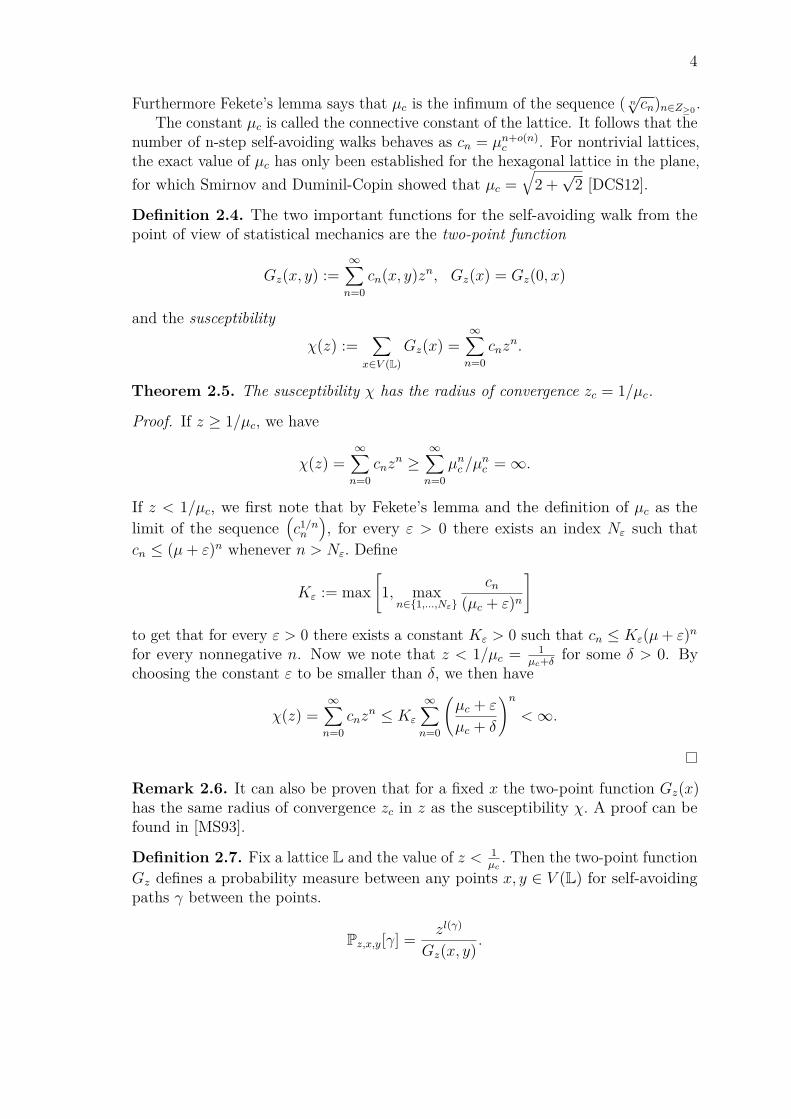
Furthermore Fekete’s lemma says that µc is the infimum of the sequence ( n√cn)n∈Z≥0 .
The constant µc is called the connective constant of the lattice. It follows that thenumber of n-step self-avoiding walks behaves as cn = µn+o(n)
c . For nontrivial lattices,the exact value of µc has only been established for the hexagonal lattice in the plane,for which Smirnov and Duminil-Copin showed that µc =
√2 +√
2 [DCS12].
Definition 2.4. The two important functions for the self-avoiding walk from thepoint of view of statistical mechanics are the two-point function
Gz(x, y) :=∞∑n=0
cn(x, y)zn, Gz(x) = Gz(0, x)
and the susceptibility
χ(z) :=∑
x∈V (L)Gz(x) =
∞∑n=0
cnzn.
Theorem 2.5. The susceptibility χ has the radius of convergence zc = 1/µc.
Proof. If z ≥ 1/µc, we have
χ(z) =∞∑n=0
cnzn ≥
∞∑n=0
µnc /µnc =∞.
If z < 1/µc, we first note that by Fekete’s lemma and the definition of µc as thelimit of the sequence
(c1/nn
), for every ε > 0 there exists an index Nε such that
cn ≤ (µ+ ε)n whenever n > Nε. Define
Kε := max[1, max
n∈1,...,Nε
cn(µc + ε)n
]
to get that for every ε > 0 there exists a constant Kε > 0 such that cn ≤ Kε(µ+ ε)nfor every nonnegative n. Now we note that z < 1/µc = 1
µc+δ for some δ > 0. Bychoosing the constant ε to be smaller than δ, we then have
χ(z) =∞∑n=0
cnzn ≤ Kε
∞∑n=0
(µc + ε
µc + δ
)n<∞.
Remark 2.6. It can also be proven that for a fixed x the two-point function Gz(x)has the same radius of convergence zc in z as the susceptibility χ. A proof can befound in [MS93].
Definition 2.7. Fix a lattice L and the value of z < 1µc. Then the two-point function
Gz defines a probability measure between any points x, y ∈ V (L) for self-avoidingpaths γ between the points.
Pz,x,y[γ] = zl(γ)
Gz(x, y) .

5
Definition 2.8. The mesh size of the lattice means the (largest) Euclidean distancebetween two neighbouring vertices of the lattice.
There is a version of definition 2.7 more suited to our needs.
Definition 2.9. Let Ω be a simply connected domain in Rd, with points x, y onthe boundary. For δ > 0 let Ωδ be the largest connected component of δL ∩ Ωand let xδ, yδ be the two sites closest to x and y. The triplet (Ωδ, xδ, yδ) is then anapproximation of (Ω, x, y).Let z > 0 and define the two-point function for Ωδ as
Gz,Ωδ(x, y) =∑
γ⊂Ωδ:xδ→yδzl(γ),
where the length of each walk γ is measured in the number of steps it takes in δL.The associated probability measure is
Pz,Ωδ,x,y[γ] = zl(γ)
Gz,Ωδ(x, y) .
Conjecture 2.10. The set of self-avoiding walks with probability distribution
Pzc,Ωδ,x,y[γ] = zl(γ)c
Gzc,Ωδ(x, y)
is called the critical self-avoiding walk. The critical SAW in the complex plane isconjectured to be conformally invariant as δ → 0. This means that there exists aprobability measure P′ on self-avoiding paths in C such that:
• For every Ω ( C and x, y ∈ ∂Ω the distribution Pzc,Ωδ,x,y[γ] converges toP′Ω,x,y[γ] as δ tends to zero.
• For every pair of open sets Ω,Ω′ ( C, boundary points x, y ∈ ∂Ω and conformalmapping f : Ω→ Ω′ we have that if γ has the law P′Ω,x,y, then f(γ) has the lawP′f(Ω),f(x),f(y). This is called conformal invariance.
The two propositions of the conjecture are illustrated in fig. 1.
Theorem 2.11. [LSW04b] If the two propositions of conjecture 2.10 are true, thenthe scaling limit of the critical self-avoiding walk is the chordal SLE8/3.
Proposition 2.12. The probability measure Pz,Ωδ,x,y[γ] exhibits a phase transitionas δ tends to 0. Here again the critical value zc is the same µ−1
c as before. Whenz < zc a walk is penalized by its length, and γδ converges to the geodesic betweenx and y as δ tends to 0 [Iof98]. When z > zc, a walk is favored by its length, andthe probability of γδ not intersecting any open set U ⊂ Ω tends to zero [DCKY14].Finally when z = zc, γδ converges to a simple random curve, and if the scaling limitof the SAW exists, this curve is the Schramm-Löwner evolution SLE8/3 [LSW04b].

6
δxδx
yδy
(Ωδ, xδ, yδ)
δ → 0
x
y
(Ω, x, y) f(x)
f(y)
(f(Ω), f(x), f(y))
f conformal
Figure 1: Conjectured conformal invariance: γδ ∼ Pzc,Ωδ,xδ,yδ −−→δ→0
γ ∼ P′Ω,x,y and if fis conformal, then the images f(γ) of the self-avoiding paths γ have the distributionthat one gets by taking the limit δ → 0 of Pzc,(f(Ω))δ,(f(x))δ,(f(y))δ : f(γ) ∼ P′f(Ω),f(x),f(y).
Figure 2: A self-avoiding walk γ on the edges of the square lattice and a self-avoidingwalk γ on the midedges of the lattice.
Definition 2.13. A midedge is the point halfway between two adjacent vertices onthe lattice, in the middle of the edge connecting these vertices.
Remark 2.14. To each N -step self-avoiding walk γ defined as above, it is possibleto associate an N − 1-step self-avoiding walk γ on midedges with
γ(i) = γ(i) + γ(i+ 1)2 , i = 0, 1, . . . , N − 1.
Between these points, the walk γ is drawn such that the walks γ and γ have thesame trajectory between points γ(0) and γ(N − 1). An example is shown in fig 2.This thesis deals with self-avoiding walks on midedges.
7
Remark 2.15. Let cn denote the number of n-step midedge-to-midedge self-avoidingwalks and let e be the number of edges adjacent to a vertex. By splitting the midedge-to-midedge walks into the first half edge, the last half edge and the n − 1-stepvertex-to-vertex midsection, one gets the bounds
2 · e− 1e
cn−1 ≤ cn ≤ 2 · e− 1e
cn−1 · (e− 1).
In particular this implies that the connective constant is the same for midedge-to-midedge and vertex-to-vertex self-avoiding walks.

8
C
vertex
midedge
Figure 3: A set of vertices V and emanating midedges
3 Complex analysis in the honeycomb latticeIn this section we introduce a parafermionic observable F , which is a weighted versionof the two-point function Gz,Ω of the self-avoiding walk, also called the partitionfunction or the generation function for an enumeration of walk lengths, in a simplyconnected region of a hexagonal discretization of the complex plane. It turns outthat discrete integrals of this observable F along the elementary contours of the duallattice vanish. This implies that the integral of F along any closed contour in thedual lattice vanishes. By choosing an appropriate contour to integrate along, wereview the proof of Nienhuis’ prediction[Nie82] that the connective constant µc forthe hexagonal lattice equals 1√
2+√
2by Smirnov and Duminil-Copin [DCS12].
3.1 Parafermionic observableConsider the complex plane C and the hexagonal lattice H with edge length 1embedded on it. Choose a set of vertices V from H such that the vertices and themidedges of the edges emanating from V form a simply connected graph Ω(V ).
Define the set Ω of midedges as follows: The midedge x belongs to Ω if at leastone of its adjacent vertices is in the set V and to the boundary ∂Ω of Ω if only oneof its adjacent vertices is in V . This makes the boundary ∂Ω a subset of Ω, meaning
9
q
p
r
v x
y
Wγ(x, y) = 0
y
x
Wγ(x, y) = 2π
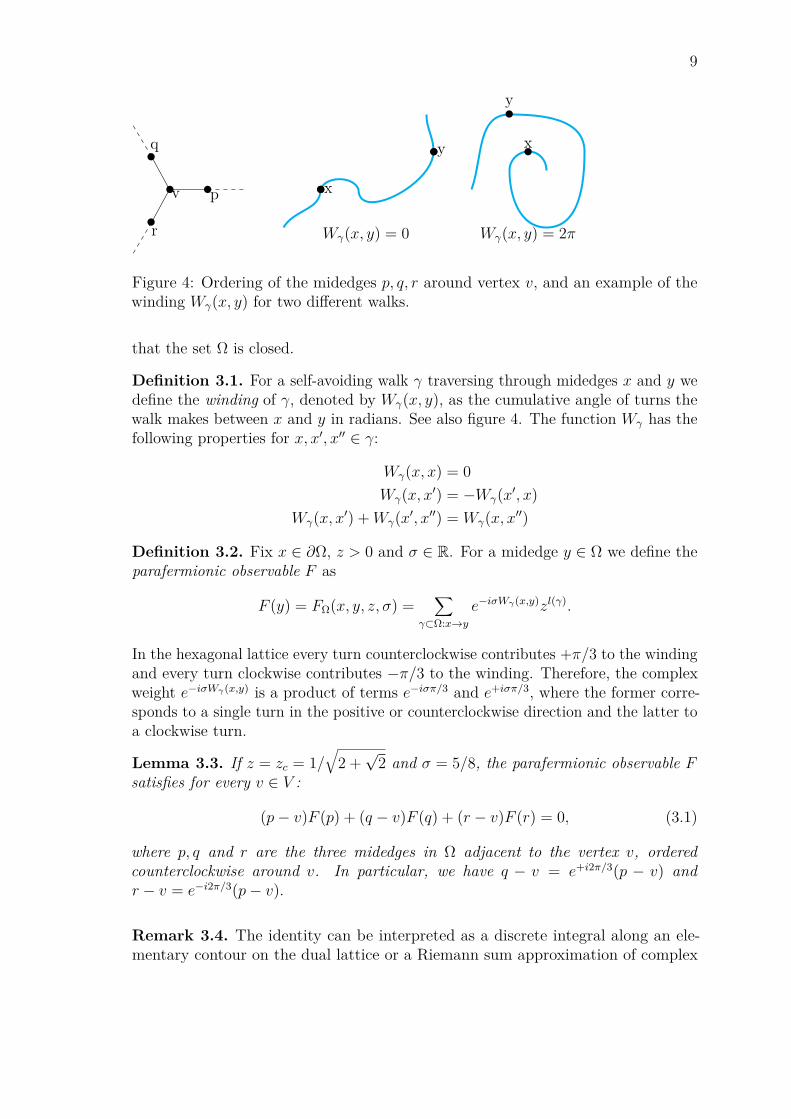
Figure 4: Ordering of the midedges p, q, r around vertex v, and an example of thewinding Wγ(x, y) for two different walks.
that the set Ω is closed.
Definition 3.1. For a self-avoiding walk γ traversing through midedges x and y wedefine the winding of γ, denoted by Wγ(x, y), as the cumulative angle of turns thewalk makes between x and y in radians. See also figure 4. The function Wγ has thefollowing properties for x, x′, x′′ ∈ γ:
Wγ(x, x) = 0Wγ(x, x′) = −Wγ(x′, x)
Wγ(x, x′) +Wγ(x′, x′′) = Wγ(x, x′′)
Definition 3.2. Fix x ∈ ∂Ω, z > 0 and σ ∈ R. For a midedge y ∈ Ω we define theparafermionic observable F as
F (y) = FΩ(x, y, z, σ) =∑
γ⊂Ω:x→ye−iσWγ(x,y)zl(γ).
In the hexagonal lattice every turn counterclockwise contributes +π/3 to the windingand every turn clockwise contributes −π/3 to the winding. Therefore, the complexweight e−iσWγ(x,y) is a product of terms e−iσπ/3 and e+iσπ/3, where the former corre-sponds to a single turn in the positive or counterclockwise direction and the latter toa clockwise turn.
Lemma 3.3. If z = zc = 1/√
2 +√
2 and σ = 5/8, the parafermionic observable Fsatisfies for every v ∈ V :
(p− v)F (p) + (q − v)F (q) + (r − v)F (r) = 0, (3.1)
where p, q and r are the three midedges in Ω adjacent to the vertex v, orderedcounterclockwise around v. In particular, we have q − v = e+i2π/3(p − v) andr − v = e−i2π/3(p− v).
Remark 3.4. The identity can be interpreted as a discrete integral along an ele-mentary contour on the dual lattice or a Riemann sum approximation of complex
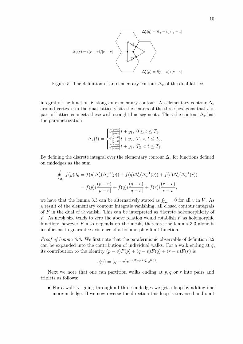
10
p
q
r
∆′v(p) = i(p− v)/|p− v|
∆′v(q) = i(q − v)/|q − v|
∆′v(r) = i(r − v)/|r − v|
Figure 5: The definition of an elementary contour ∆v of the dual lattice
integral of the function F along an elementary contour. An elementary contour ∆v
around vertex v in the dual lattice visits the centers of the three hexagons that v ispart of lattice connects these with straight line segments. Thus the contour ∆v hasthe parametrization
∆v(t) =
i (p−v)|p−v| t+ y1, 0 ≤ t ≤ T1,
i (q−v)|q−v| t+ y2, T1 < t ≤ T2,
i (r−v)|r−v| t+ y3, T2 < t ≤ T3.
By defining the discrete integral over the elementary contour ∆v for functions definedon midedges as the sum∮
∆v
f(y)dy = f(p)∆′v(∆−1v (p)) + f(q)∆′v(∆−1
v (q)) + f(r)∆′v(∆−1v (r))
= f(p)i(p− v)|p− v|
+ f(q)i(q − v)|q − v|
+ f(r)i(r − v)|r − v|
,
we have that the lemma 3.3 can be alternatively stated as∮
∆v= 0 for all v in V . As
a result of the elementary contour integrals vanishing, all closed contour integralsof F in the dual of Ω vanish. This can be interpreted as discrete holomorphicity ofF . As mesh size tends to zero the above relation would establish F as holomorphicfunction; however F also depends on the mesh, therefore the lemma 3.3 alone isinsufficient to guarantee existence of a holomorphic limit function.
Proof of lemma 3.3. We first note that the parafermionic observable of definition 3.2can be expanded into the contribution of individual walks. For a walk ending at q,its contribution to the identity (p− v)F (p) + (q − v)F (q) + (r − v)F (r) is
c(γ) = (q − v)e−iσWγ(x,q)zl(γ).
Next we note that one can partition walks ending at p, q or r into pairs andtriplets as follows:
• For a walk γ1 going through all three midedges we get a loop by adding onemore midedge. If we now reverse the direction this loop is traversed and omit

11
the last midedge of the reversed loop, we associate to γ1 a walk γ2 that hasthe same trajectory up to v and then goes through the loop from v to v in theother direction. Thus one can group the walks visiting all three midedges inpairs.
• If a walk γ1 visits only one of the midedges, we get walks γ2 and γ3 by prolongingthe walk with one step. The reverse is also true: a walk visiting two midedgesis naturally associated to a walk visiting only one midedge by erasing its laststep. Hence, walks visiting one or two midedges can be grouped in triplets.
The following step is to show that the contribution of every pair and triplet toequation (3.1) equals zero, which completes the proof of the lemma. For both pairsand triplets we can without loss of generality assume that the walk γ1 first visits themidedge p.
In the case of pairs: Let γ1 end at q and γ2 end at r. The walks γ1 and γ2 agreeuntil p after which they go through an almost complete loop in opposite directions.This implies that l(γ1) = l(γ2) andWγ1(x, q) = Wγ1(x, p)− 4π/3
Wγ2(x, r) = Wγ1(x, p) + 4π/3.
For the windings of γ1 and γ2 we have used the fact that x is on the boundary of thesimply connected set Ω, making it impossible for the walk to wind around x.
q
p
r
vγ1
q
p
r
vγ2
Figure 6: An illustration of a pair of walks visiting p, q and r.
The total contribution of the pair to relation (3.1) is
c(γ1) + c(γ2) = (q − v)e−iσWγ1 (x,q)zl(γ1) + (r − v)e−iσWγ2 (x,r)zl(γ2)
= (p− v)zl(γ1)e−iσWγ1 (x,p)(ei2π/3
(eiσπ/3
)4+ e−i2π/3
(e−iσπ/3
)4)
= C(ei2π/3eiσ4π/3 + e−i2π/3e−iσ4π/3
).
The sum of a complex number ξ and and its conjugate ξ vanishes exactly when ξ hasno real component. In order to guarantee that the sum cancels out we must choose
12
σ such that
ei2π/3eiσ4π/3 = ±i2π/3 + 4πσ/3 = π/2 + nπ, n ∈ Z
σ = 6n− 18 , n ∈ Z.
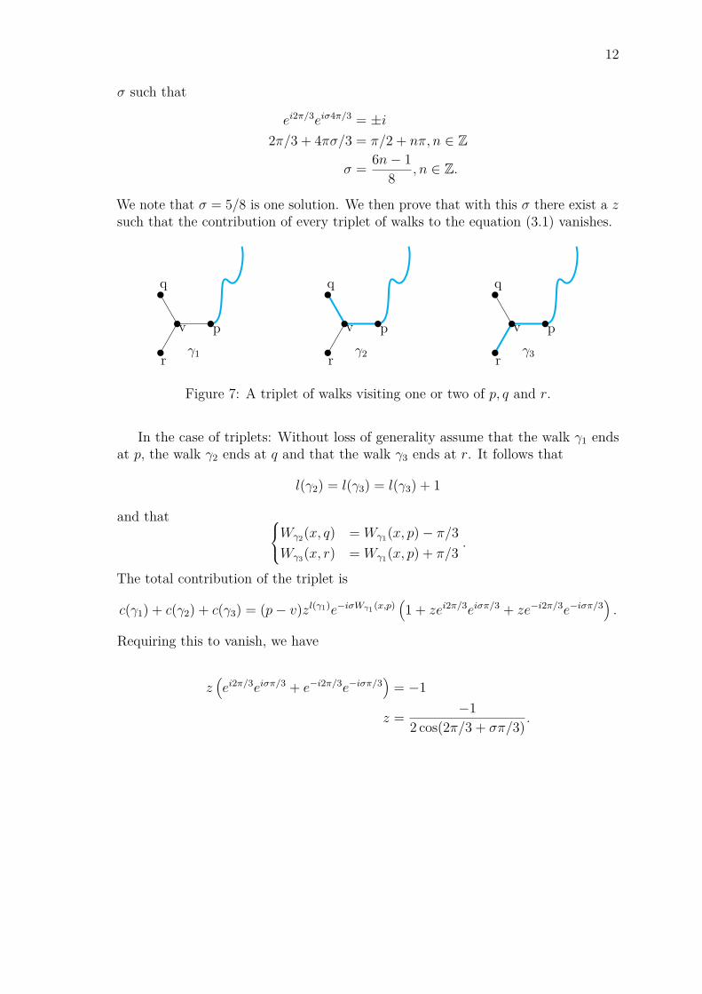
We note that σ = 5/8 is one solution. We then prove that with this σ there exist a zsuch that the contribution of every triplet of walks to the equation (3.1) vanishes.
q
p
r
vγ1
q
p
r
vγ2
q
p
r
vγ3
Figure 7: A triplet of walks visiting one or two of p, q and r.
In the case of triplets: Without loss of generality assume that the walk γ1 endsat p, the walk γ2 ends at q and that the walk γ3 ends at r. It follows that
l(γ2) = l(γ3) = l(γ3) + 1
and that Wγ2(x, q) = Wγ1(x, p)− π/3Wγ3(x, r) = Wγ1(x, p) + π/3
.
The total contribution of the triplet is
c(γ1) + c(γ2) + c(γ3) = (p− v)zl(γ1)e−iσWγ1 (x,p)(1 + zei2π/3eiσπ/3 + ze−i2π/3e−iσπ/3
).
Requiring this to vanish, we have
z(ei2π/3eiσπ/3 + e−i2π/3e−iσπ/3
)= −1
z = −12 cos(2π/3 + σπ/3) .
13
Plugging in σ = 6n−18 , n ∈ Z, we get a family of solutions
σ = 6n− 18 , z =
1√2−√
2, n ≡ 0 mod 8
1√2+√
2, n ≡ 1 mod 8
1√2+√
2, n ≡ 2 mod 8
1√2−√
2, n ≡ 3 mod 8
− 1√2−√
2, n ≡ 4 mod 8
− 1√2+√
2, n ≡ 5 mod 8
− 1√2+√
2, n ≡ 6 mod 8
− 1√2−√
2, n ≡ 7 mod 8
. (3.2)
z = 1/√
2 +√
2, σ = 5/8 is what we get when n equals 1, which completes theproof.
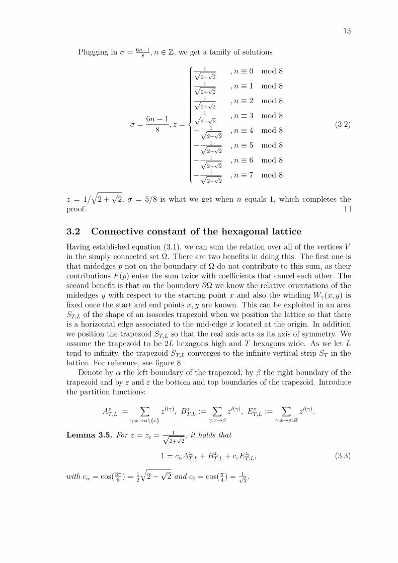
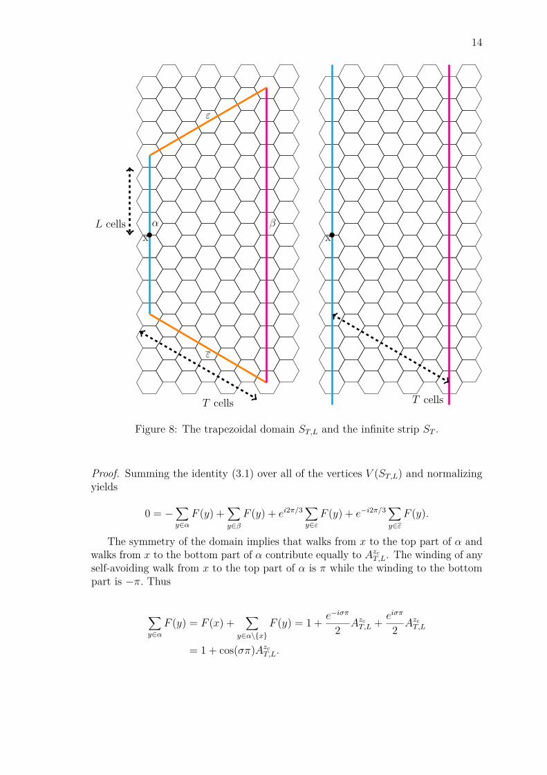
3.2 Connective constant of the hexagonal latticeHaving established equation (3.1), we can sum the relation over all of the vertices Vin the simply connected set Ω. There are two benefits in doing this. The first one isthat midedges p not on the boundary of Ω do not contribute to this sum, as theircontributions F (p) enter the sum twice with coefficients that cancel each other. Thesecond benefit is that on the boundary ∂Ω we know the relative orientations of themidedges y with respect to the starting point x and also the winding Wγ(x, y) isfixed once the start and end points x, y are known. This can be exploited in an areaST,L of the shape of an isosceles trapezoid when we position the lattice so that thereis a horizontal edge associated to the mid-edge x located at the origin. In additionwe position the trapezoid ST,L so that the real axis acts as its axis of symmetry. Weassume the trapezoid to be 2L hexagons high and T hexagons wide. As we let Ltend to infinity, the trapezoid ST,L converges to the infinite vertical strip ST in thelattice. For reference, see figure 8.
Denote by α the left boundary of the trapezoid, by β the right boundary of thetrapezoid and by ε and ε the bottom and top boundaries of the trapezoid. Introducethe partition functions:
AzT,L :=∑
γ:x→α\xzl(γ), Bz
T,L :=∑
γ:x→βzl(γ), Ez
T,L :=∑
γ:x→ε∪εzl(γ).
Lemma 3.5. For z = zc = 1√2+√
2, it holds that
1 = cαAzcT,L +Bzc
T,L + cεEzcT,L, (3.3)
with cα = cos(3π8 ) = 1
2
√2−√
2 and cε = cos(π4 ) = 1√2 .
14
α
ε
β
ε
xL cells
T cells T cells
x
Figure 8: The trapezoidal domain ST,L and the infinite strip ST .
Proof. Summing the identity (3.1) over all of the vertices V (ST,L) and normalizingyields
0 = −∑y∈α
F (y) +∑y∈β
F (y) + ei2π/3∑y∈ε
F (y) + e−i2π/3∑y∈ε
F (y).
The symmetry of the domain implies that walks from x to the top part of α andwalks from x to the bottom part of α contribute equally to AzcT,L. The winding of anyself-avoiding walk from x to the top part of α is π while the winding to the bottompart is −π. Thus
∑y∈α
F (y) = F (x) +∑
y∈α\xF (y) = 1 + e−iσπ
2 AzcT,L + eiσπ
2 AzcT,L
= 1 + cos(σπ)AzcT,L.
15
Above we have used the fact that the only self-avoiding walk from x to x is thetrivial one of length 0, hence F (x) = 1. Similarly to α, the winding from x to anymid-edge in β(resp. ε and ε) is 0( resp. 2π
3 and −2π3 ), therefore∑
y∈βF (y) = Bzc
T,L
and, since by symmetry ε and ε must contribute equally to EzcT,L,
ei2π/3∑y∈ε
F (y) + e−i2π/3∑y∈ε
F (y) = e−i(1−σ)2π/3
2 EzcT,L + ei(1−σ)2π/3
2 EzcT,L
= cos((1− σ)2π/3)EzcT,L.
Thus, the identity (3.1) leads us to the equation
1 = cos ((1− σ)π)AzcT,L +BzcT,L + cos ((1− σ)2π/3)Ezc
T,L,
where σ and zc belong to the solution family (3.2). In particular σ = 5/8,zc = 1/
√2 +√
2 gives the values cα, cε in the statement of the lemma.
Remark 3.6. The proof of the connective constant will rely on zc and cα beingpositive. These two conditions imply that only the solutions of (3.1) where n ≡ 1, 2mod 8 in (3.2) are possible. Looking at these solutions, we see that zc =
√2 +√
2−1
is uniquely determined.
Note that the sequences(AzT,L
)L>0
and(BzT,L
)L>0
are increasing in L and arebounded for z ≤ zc thanks to their monotonicity in z and the identity (3.3). Thereforethey have the limits
AzT := limL→∞
AzT,L, BzT := lim
L→∞BzT,L.
By identity (3.3) we can deduce that(EzcT,L
)L>0
decreases and converges to alimit Ezc
T := limL→∞EzcT,L. Letting L tend to infinity in the identity (3.3), we arrive
at1 = cαA
zcT +Bzc
T + cεEzcT . (3.4)
Proof of µ =√
2 +√
2. We prove first that χ(zc) = ∞, and hence µ ≥√
2 +√
2.Suppose first that for some T, Ezc
T > 0. As noted before, EzcT,L decreases in L and so
χ(zc) ≥∑L>0
EzcT,L ≥
∑L>0
EzcT = +∞.
Assuming on the contrary that EzcT = 0 for all T , the equation (3.4) renders to
1 = cαAzcT +Bzc
T .
16
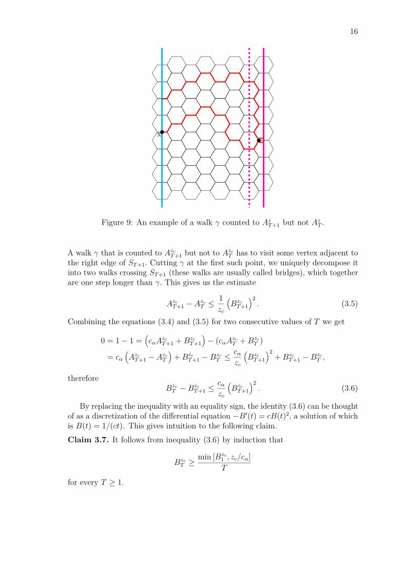
x
Figure 9: An example of a walk γ counted to AzT+1 but not AzT .
A walk γ that is counted to AzcT+1 but not to AzcT has to visit some vertex adjacent tothe right edge of ST+1. Cutting γ at the first such point, we uniquely decompose itinto two walks crossing ST+1 (these walks are usually called bridges), which togetherare one step longer than γ. This gives us the estimate
AzcT+1 − AzcT ≤1zc
(BzcT+1
)2. (3.5)
Combining the equations (3.4) and (3.5) for two consecutive values of T we get
0 = 1− 1 =(cαA
zcT+1 +Bzc
T+1
)− (cαAzcT +Bzc
T )
= cα(AzcT+1 − AzcT
)+Bzc
T+1 −BzcT ≤
cαzc
(BzcT+1
)2+Bzc
T+1 −BzcT ,
thereforeBzcT −Bzc
T+1 ≤cαzc
(BzcT+1
)2. (3.6)
By replacing the inequality with an equality sign, the identity (3.6) can be thoughtof as a discretization of the differential equation −B′(t) = cB(t)2, a solution of whichis B(t) = 1/(ct). This gives intuition to the following claim.Claim 3.7. It follows from inequality (3.6) by induction that
BzcT ≥
min [Bzc1 , zc/cα]T
for every T ≥ 1.
17
Proof of claim 3.7 Clearly Bzc1 ≥ min
[Bzc
1 ,zccα
]so the identity holds for T = 1.
Denote now min[Bzc
1 ,zccα
]by m and assume that the identity Bzc
T ≥ mTholds for some
T ≥ 1. Substituting m and the induction assumption into the inequality (3.6) wehave
m
T−Bzc
T+1 ≤
(BzcT+1
)2
m
Solving this with respect to BzcT+1 yields
BzcT+1 ≥ m
√ 1T
+ 14 −
12
.Finally note that
√1T
+ 14 −
12 ≥
1T+1 holds for T strictly greater than 0, thus
BzcT+1 ≥
m
T + 1 ,
proving the claim.
The claim 3.7 gives the estimate
χ(zc) ≥ m∑T>0
1T
= +∞.
This completes the proof for the estimate µ ≥ z−1c =
√2 +√
2.It remains to prove the opposite inequality µ ≤ z−1
c . To estimate the partitionfunction from above, we will decompose self-avoiding walks into bridges. A bridge ofwidth T is a self-avoiding walk in ST from one side to the opposite side, defined upto vertical translation. The partition function of bridges of width T is Bz
T , which isat most 1 by 3.4. Noting that a bridge of width T has length at least T , we obtainfor z < zc
BzT ≤
(z
zc
)TBzcT ≤
(z
zc
)T.
Thus for z < zc the sum ∑T>0B
zT converges and so does the product∏
T>0 (1 +BzT ) < ∏
T>0 eBzT . We will next use the fact that any self-avoiding walk
can be canonically decomposed into a sequence of bridges of widths T−i < . . . < T−1and T0 > . . . > Tj . In addition if one fixes the first midedge, the first vertex and thelast midedge visited by the walk, the decomposition uniquely determines the walk.Noting that in the hexagonal lattice the walk will take one step between the bridges
18
of the decomposition and that z < 1 we have
χ(z) ≤ 4∑
T−i<...<T−1T0>...>Tj
zi+j
j∏k=−i
BzTk
≤ 4∑
T−i<...<T−1T0>...>Tj
j∏k=−i
BzTk
= 4(∏T>0
1 +BzT
)2
<∞.
The procedure for decomposing the walk into bridges goes as follows. First assumethe walk γ is a half-plane self-avoiding walk, i.e. the starting point has extremal realpart. Without loss of generality assume the start has minimal real part. To get thefirst bridge γ0 of width T0, take the one visited last of the vertices with maximal realpart in γ. If this vertex is visited after N0 steps, the bridge γ0 consists of γ up to theN th
0 vertex and the midedge horizontally adjacent to it. To get the second bridge γ1of width T1 < T0, start from the N0 + 1th step γ(N0 + 1) and consider the last vertexin γ after that with a minimal real part, say the N th
1 vertex. The bridge γ1 will thenbe trajectory from γ(N0 + 1) to the N th
1 vertex in γ with a half-step extension in thenegative direction in the end. Now the part of γ starting from the point γ(N1 + 1) isa half-plane self-avoiding walk and we can repeat the steps performed before. Usingthis algorithm recursively yields a sequence of bridges of widths T0 > T1 > . . . > Tjthat characterizes the half-plane walk up to the last step. It should be noted that thetotal length of the bridges will be j steps less than the length of the original walk γ.
Finally note that any self-avoiding walk in the plane can be divided into twohalf-plane walks. Let the first vertex with the maximal real part in a walk γ in theplane be the N th one. This means that the walk γ up to the N th vertex extended byone half-step in the positive direction is a half-plane walk and the part of γ from theγ(N + 1) to the end is a half-plane walk. The procedure for decomposing half-planewalks into bridges can then be applied for both of these to get sequences of bridgesof widths T−i < Ti−1 < . . . < T−1 and T0 > T1 > . . . > Tj. The factor 4 in equation(3.2) is a result of the two options for the first vertex of the walk and the two optionsfor the last midedge of the walk, left undefined by the bridge decomposition. For anexample, see figure 10.

19
Figure 10: The decomposition of the walk on the left into bridges, on the right theblue bridges correspond to negative indices and the red ones to non-negative indices.In the example T−1 = 7 > T−2 = 2 > T−3 = 1 > T−4 = 0 and T0 = 8 > T1 = 4 >T2 = 3 > T3 = 1.
20
4 Transfer matricesThe idea of this chapter is to show that self-avoiding walks in vertical cylinder domainscan be canonically described by the sequence of configurations indexed by height thatthe walk assumes at different layers of the cylinder. We then express the generatingfunction Gz similar to the one in the first chapter in terms of a transfer matrix forthe set of configurations. Using the probability measure associated to the generatingfunction allows the calculation of edge visiting probabities in the cylinder sets. Inparticular the probability of the walk returning to the boundary of the cylinder canbe calculated using the generating matrix, and as the height of the cylinder tendsto infinity this probability converges to a value that can also be calculated. Thisprovides one way to approximate the scaling limit of the self-avoiding walk. We alsoshow that the limit measure on the set of walks conditioned to progress upward onthe infinite cylinder is Markovian. The idea of using matrices to express the partitionfunctions of SA walks in strips is not entirely new, for example Alm and Janson useda similar approach in 1990 [AJ90].
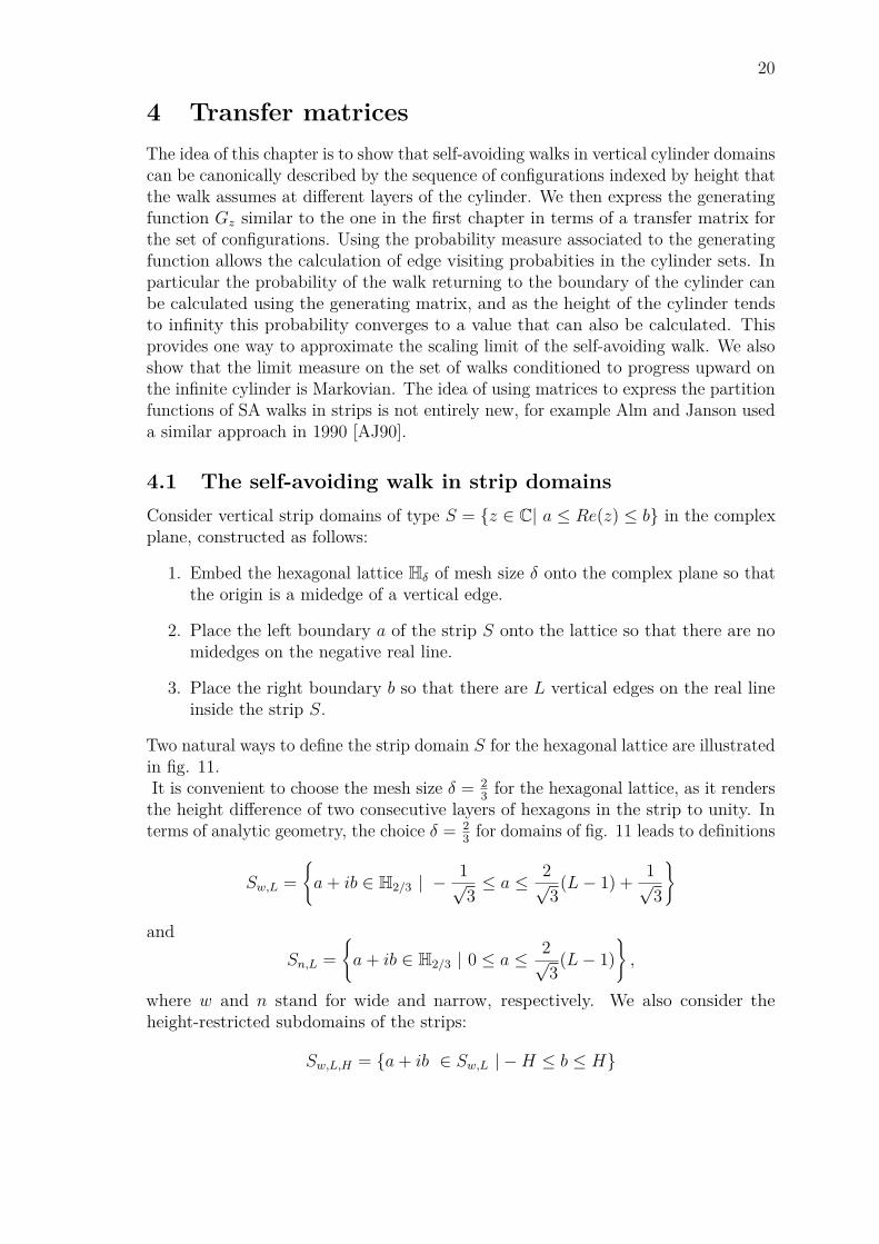
4.1 The self-avoiding walk in strip domainsConsider vertical strip domains of type S = z ∈ C| a ≤ Re(z) ≤ b in the complexplane, constructed as follows:
1. Embed the hexagonal lattice Hδ of mesh size δ onto the complex plane so thatthe origin is a midedge of a vertical edge.
2. Place the left boundary a of the strip S onto the lattice so that there are nomidedges on the negative real line.
3. Place the right boundary b so that there are L vertical edges on the real lineinside the strip S.
Two natural ways to define the strip domain S for the hexagonal lattice are illustratedin fig. 11.It is convenient to choose the mesh size δ = 2
3 for the hexagonal lattice, as it rendersthe height difference of two consecutive layers of hexagons in the strip to unity. Interms of analytic geometry, the choice δ = 2
3 for domains of fig. 11 leads to definitions
Sw,L =a+ ib ∈ H2/3 | −
1√3≤ a ≤ 2√
3(L− 1) + 1√
3
andSn,L =
a+ ib ∈ H2/3 | 0 ≤ a ≤ 2√
3(L− 1)
,
where w and n stand for wide and narrow, respectively. We also consider theheight-restricted subdomains of the strips:
Sw,L,H = a+ ib ∈ Sw,L | −H ≤ b ≤ H

21
Sn,L
−7i
−6i
−5i
−4i
−3i
−2i
−1i0i
1i
2i
3i
4i
5i
6i
7i
Sw,L
Figure 11: Examples of the strip domains Sn,L and Sw,L for L = 5.
22
andSn,L,H = a+ ib ∈ Sn,L |H ≤ b ≤ H .
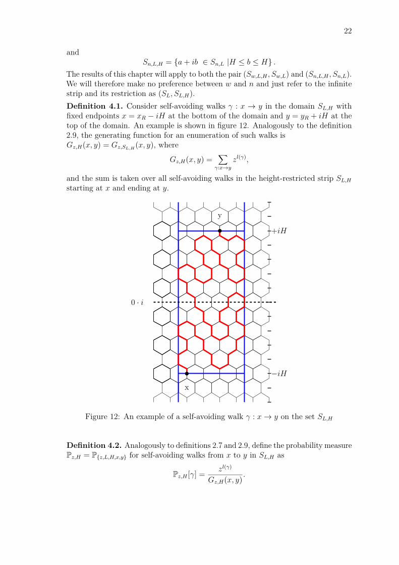
The results of this chapter will apply to both the pair (Sw,L,H , Sw,L) and (Sn,L,H , Sn,L).We will therefore make no preference between w and n and just refer to the infinitestrip and its restriction as (SL, SL,H).Definition 4.1. Consider self-avoiding walks γ : x → y in the domain SL,H withfixed endpoints x = xR − iH at the bottom of the domain and y = yR + iH at thetop of the domain. An example is shown in figure 12. Analogously to the definition2.9, the generating function for an enumeration of such walks isGz,H(x, y) = Gz,SL,H (x, y), where
Gz,H(x, y) =∑γ:x→y
zl(γ),
and the sum is taken over all self-avoiding walks in the height-restricted strip SL,Hstarting at x and ending at y.
0 · i
+iH
−iHx
y
Figure 12: An example of a self-avoiding walk γ : x→ y on the set SL,H
Definition 4.2. Analogously to definitions 2.7 and 2.9, define the probability measurePz,H = Pz,L,H,x,y for self-avoiding walks from x to y in SL,H as
Pz,H [γ] = zl(γ)
Gz,H(x, y) .

23
The main result of this chapter is:
Theorem 4.3. Fix z > 0 and L ∈ Z>0. Then there exists a vector space V , a linearoperator T = Tz : V → V and vectors vx, vy ∈ V such that
1. The generating function Gz,H can be expressed as
Gz,H(x, y) = vTy THvx.
2. For each midedge e = a+ ib, where b ∈ [−H,−H] and a is such that a+ ib isa midedge in SL,H , there exists a linear operator P (a) such that:
Pz,H [e ∈ γ] =vTy T
H−y2 P (a)T H+y
2 vx
vTy THvx
.
3. The sequence (Pz,H)H∈N converges weakly towards a limit measure Pz as Htends to infinity.
4. The limit measure Pz is Markovian in the sense specified in section 4.5.
By utilizing the results of this chapter, chapter 5 seeks to provide computationalsupport for conjecture 2.10, first formulated by physicists in the 1980s and refinedby theorem 2.11 by Lawler, Schramm and Werner in [LSW04b].
4.2 A fundamental vector spaceDefinition 4.4. A level is a horizontal line with an integer imaginary coordinate,i.e. ∪a∈R a+ ni | n ∈ Z. By the definitions of sets SL,H and SL, each level halvesa layer of hexagons in the lattice.
Definition 4.5. Consider self-avoiding walks in the set SL,H . At a level in SL,Hkeep track of
• the real coordinates of the edges the walk uses.
• the real coordinates of the pairs of edges joined by the trajectory of the walkbelow the level.
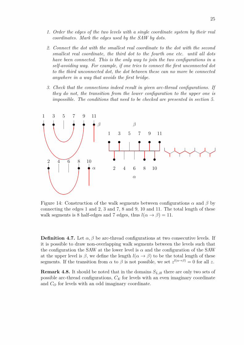
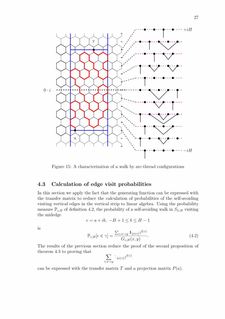
This results in an arc-thread configuration consisting of an edge and a possibly emptyset of pairs of edges, where the single edge, or thread, tells the place where the walkfirst intersected the level and the pairs of edges, or arcs, correspond to U-shapedloops in the trajectory of the walk below the level. An example of how to form anarc-thread configuration is illustrated in fig. 13. Figure 15 shows an example of thisprocedure applied to all levels of the set SL,H .
Proposition 4.6. The trajectory of a self-avoiding walk between two consecutivelevels in the vertical strip is uniquely determined by the arc-thread configurations ofthe levels.Proof. This results from the properties of the hexagonal lattice. The only possibleway of joining the configurations can be algorithmically expressed as follows:

24
−2i
+iH
−iHa
b
A)
−2i
−iH
B)
a
−2iC)
Figure 13: A)a SAW B)the same SAW with only the part below a level visible C)thearc-thread configuration of the SAW at that level
25
1. Order the edges of the two levels with a single coordinate system by their realcoordinates. Mark the edges used by the SAW by dots.
2. Connect the dot with the smallest real coordinate to the dot with the secondsmallest real coordinate, the third dot to the fourth one etc. until all dotshave been connected. This is the only way to join the two configurations in aself-avoiding way. For example, if one tries to connect the first unconnected dotto the third unconnected dot, the dot between these can no more be connectedanywhere in a way that avoids the first bridge.
3. Check that the connections indeed result in given arc-thread configurations. Ifthey do not, the transition from the lower configuration to the upper one isimpossible. The conditions that need to be checked are presented in section 5.
β
1 3 5 7 9 11
α
2 4 6 8 10
1 3 5 7 9 11
β
2 4 6 8 10α
Figure 14: Construction of the walk segments between configurations α and β byconnecting the edges 1 and 2, 3 and 7, 8 and 9, 10 and 11. The total length of thesewalk segments is 8 half-edges and 7 edges, thus l(α→ β) = 11.
Definition 4.7. Let α, β be arc-thread configurations at two consecutive levels. Ifit is possible to draw non-overlapping walk segments between the levels such thatthe configuration the SAW at the lower level is α and the configuration of the SAWat the upper level is β, we define the length l(α→ β) to be the total length of thesesegments. If the transition from α to β is not possible, we set zl(α→β) = 0 for all z.
Remark 4.8. It should be noted that in the domains SL,H there are only two sets ofpossible arc-thread configurations, CE for levels with an even imaginary coordinateand CO for levels with an odd imaginary coordinate.

26
Definition 4.9. We are now ready to define the transfer matrix T . Without lossof generality, consider only transitions between two consecutive even levels. Letα, β ∈ CE and vα, vβ be their vector forms in the set VE of formal linear combinationsof CE. The transfer matrix T = Tz is defined elementwise as the sum over allconfigurations in CO:
vTβ Tvα = T(β,α) =∑δ∈CO
zl(α→δ)zl(δ→β).
Note that the transfer matrix element T(β,α) is the generating, or partition, functionfor an enumeration of sets of walk segments connecting lower configuration α toconfiguration β two levels above α.
Definition 4.10. By swapping CE and CO in the above definition one can alsoconstruct a transfer matrix for two consecutive odd levels. For more detailed analysis,we define the transfer matrices between two consecutive levels. Let α, β ∈ CE, δ ∈ COand vα, vβ correspond to α, β in the set VE, vδ correspond to δ in the set VO of formallinear combinations of CO. Set the even-to-odd transfer matrix elements to be
T (e→ o)(δ,α) = T ?(δ,α) = vTδ T?vα = zl(α→δ)
and the odd-to-even transfer matrix elements to be
T (o→ e)(β,δ) = T (β,δ) = vTδ Tvβ = zl(δ→β).
By the definition of matrix product, this yields
T(β,α) = (T T ?)(β,α).
Now we are ready to prove the first part of theorem 4.3.
Proof for Gz,H(x, y) = vTy THvx:
Assume without loss of generality that H is even. Recall the proposition 4.6 andnote that it implies a walk in the strip SL,H is uniquely characterized by fixing itsarc-thread configurations at every level. Further note that length of the walk equalsthe sum of lengths of bridges the walk makes between consecutive levels. By usingthe short-hand x for the starting configuration with only a thread of real coordinatexR and y for the final configuration with only a thread of real coordinate yR, thefunction Gz,H = Gz,H(x, y) can be re-expressed as
Gz,H =∑γ:x→y
zl(γ)
=∑
α1,α2,...αH−1∈CEδ1,δ2,...,δH∈CO
zl(x→δ1)zl(δ1→α1)zl(α1→δ2) . . . zl(δH−1→αH−1)zl(αH−1→δH)zl(δH→y)
=∑
α1,α2,...αH−1∈CET(y,αH−1)T(αH−1,αH−2) . . . T(α2,α1)T(α1,x)
= TH(y,x) = vTy THvx.
(4.1)
27
0 · i
+iH
−iH
x
y
Figure 15: A characterization of a walk by arc-thread configurations
4.3 Calculation of edge visit probabilitiesIn this section we apply the fact that the generating function can be expressed withthe transfer matrix to reduce the calculation of probabilities of the self-avoidingvisiting vertical edges in the vertical strip to linear algebra. Using the probabilitymeasure Pz,H of definition 4.2, the probability of a self-avoiding walk in SL,H visitingthe midedge
e = a+ ib, −H + 1 ≤ b ≤ H − 1
isPz,H [e ∈ γ] =
∑γ:x→y 1[e∈γ]z
l(γ)
Gz,H(x, y) . (4.2)
The results of the previous section reduce the proof of the second proposition oftheorem 4.3 to proving that ∑
γ:x→y1[e∈γ]z
l(γ)
can be expressed with the transfer matrix T and a projection matrix P (a).

28
Proof of Thm. 4.3.2. For simplicity, assume that b and H are both even. We makethree remarks. The first remark is that according to definition 4.9 the argumentsfor the function Gz,H(·, ·) do not need to be points, they can be any arc-threadconfigurations. The second remark is that the generating function Gz,H is translationinvariant, if we move the cylinder domain SL,H an even number of levels up or downalong the vertical strip SL. The third remark is that the walk γ can be split intotwo parts, a self-avoiding set of walk segments γ(1) starting from x and ending insome arc-thread configuration, say α, below the level b and a self-avoiding set ofwalk segments γ(2) above the level b, starting from the configuration α and endingin y. By translating γ(1) and γ(2) to the sets SL,(H+b)/2 and SL,(H−b)/2, respectively,and applying the arguments of subsection 4.2, it follows that γ(1) has the generatingfunction T
H+b2
(α,x) and γ(2) has the generating function TH−b
2(y,α) . The numerator on the
right-hand side of the equation (4.2) can be expressed by summing the product ofpartition functions for walks γ(1) and γ(2) over all the configurations α at level b:
∑γ:x→y
1[e∈γ]zl(γ) =
∑(α:a∈α)
TH−b
2(y,α)T
H+b2
(α,x).
By introducing projection matrices P (a) for the set of configurations, defined entrywiseby
vTβ P (a)vα = P (a)(β,α) =
1, if β = α and a ∈ α0, else
the condition a ∈ α can be omitted from the sum:∑γ:x→y
1[e∈γ]zl(γ) =
∑α
TH−b
2(y,α)P (a)(α,α)T
H+b2
(α,x)
=∑α,β
TH−b
2(y,β)P (a)(β,α)T
H+b2
(α,x).
Finally using the definition of matrix product yields the result of theorem 4.3
Pz,H [e ∈ γ] =
(TH−b
2 P (a)T H+b2)
(y,x)
TH(y,x)
=vTy T
H−b2 P (a)T H+b
2 vx
vTy THvx
.
It is straightforward to generalize the probability formula for a pair of edges
e1 = a1 + ib1, e2 = a2 + ib2, b1 ≤ b2.
For simplicity assume that H, b1 and b2 are all even. The walk can now be dividedinto three sets of walk segments, γ(1) below the level b1, γ(2) between the levels b1
29
and b2 and γ(3) above the level b2. Using the same arguments as in the proof for theprobability of visiting single edge yields
Pz,H [e1, e2 ∈ γ] =vTy T
H−b22 P (a2)T
b2−b12 P (a1)T
H+b12 vx
vTy THvx
.
Remark 4.11. The same technique works for expressing the probability of visitingany set vertical of edges (ej)nj=1, ej = aj + ibj with the rule bj ≤ bj+1.
For the next section, we also need to consider the equation (4.2) with odd b.Recall the notation from definition 4.10 where T ? denotes the transfer matrix froman even level to the following odd one and T denotes the transfer matrix from anodd level to the following even one. By splitting the walk to the segments γ(1) belowlevel b − 1, γ(2) between levels b − 1 to b, γ(3) from b to b + 1 and γ(4) above levelb+ 1, the same reasoning as before yields for e = a+ ib
Pz,H [e ∈ γ] =vTy T
H−1−b2 T P (a)T ?T H−1+b
2 vx
vTy THvx
.
Finally we give the same formulas for e = a+ ib when H is odd. First when b iseven,
Pz,H [e ∈ γ] =vTy T
TH−1−b
2 P (a)T H−1+b2 T ?vx
vTy TTH−1T ?vx
,
and similarly when both b and H are odd:
Pz,H [e ∈ γ] =vTy T
TH−2−b
2 T ?P (a)T T H−2+b2 T ?vx
vTy TTH−1T ?vx
.
4.4 Weak convergence to a limit measureIn this section we first present a criterion that guarantees weak convergence for asequence of probability measures on a metric space X given that the probabilitiesconverge for a certain family that belongs to the Borel σ-algebra of X. We showthat the spaces SI with a finite set of values S and a countable number of indices Iare metric spaces, and in addition that they are separable and compact. We thenapply the first criterion to cylinder events and use Prokhorov’s theorem to provethat the convergence of probabilities of cylinder events in the sets SI characterizesweak convergence. Finally we prove that the sequence (Pz,H)H∈N converges to a limitmeasure Pz by showing that the probabilities of cylinder events converge.
Proposition 4.12. Let (X, ρ) be a metric space and B = B(X) its Borel σ-algebra.Suppose E ⊂ B is a collection such that
• E is stable under finite intersections, i.e. E1, E2 ∈ E implies E1 ∩ E2 ∈ E
• Any open set U ⊂ X is a countable union of sets from E:
U =⋃i∈N
Ei, where Ei ∈ E .

30
Then a sequence of probability measures (νh)h∈N of probability measures on X con-verges weakly to a probability measure ν if for all E ∈ E we have νh[E]→ ν[E].
Proof. If E1, E2, . . . Em ∈ E , then their intersection ⋂mi=1Ei is also in E . By the
inclusion-exclusion formula
νh[m⋃i=1
Ei] =∑
J⊂1,2,...,mJ 6=∅
(−1)|J |νh[⋂j∈J
Ej].
The finite intersections of sets in E belong to the family E and thus the inclusion-exclusion formula converges to
∑J⊂1,2,...,m
J 6=∅
(−1)|J |ν[⋂j∈J
Ej] = ν[m⋃i=1
Ei].
If a set U ⊂ X is open, by the second condition there is a countable union of setsin Ei in the collection E such that U = ⋃∞
i=1 Ei. Convergence of the sequence ofprobability measures for sets E ∈ E gives
ν[m⋃i=1
Ei] = limh→∞
νh[m⋃i=1
Ei] ≤ lim infh→∞
νh[U ].
On the other hand, (⋃mi=1Ei)m∈N is an increasing sequence in the sense that⋃mi=1Ei ⊂
⋃m+1i=1 Ei with limit U so the left hand side tends to ν[U ] by monotone
approximation of measures. The equation is now in a form that characterizes weakconvergence of νh to ν by the Portmanteau theorem.
Theorem 4.13 (Prokhorov’s theorem). [Shi95, p. 318] Let (S, ρ) be a separablemetric space. Then for every sequence (µn)n∈N of probability measures on (S, ρ) thereexists a weakly converging subsequence if and only if the set of probability measureson (S, ρ) is tight.
Remark 4.14. The set of probability measures on a metric separable space (S, ρ)is tight if the space is compact.
Lemma 4.15. Let S be a finite set of values and I a countable set of indices. Definethe metric ρ on SI as:
ρ(ω, ω′) =∑j∈I
2−j1[ωj 6=ω′j ] =∑
j:ωj 6=ω′j2−j.
This leads to a complete, separable and compact metric space(SI , ρ
).
Proof. It can be assumed without loss of generality that I = N.
• ρ is a metric on SI :By the definition of ρ, we have
0 ≤ ρ(ω, ω′) ≤∑i∈N
2−i = 1.
31
Thus ρ satisfies the non-negativity axiom of metrics and the space (SN, ρ) isbounded with diameter 1.To prove the identity of indiscernibles for ρ, note that by definition of ρ(ω, ω′) =0 is equivalent with ωi = ω′i for all i in N, which means that ω = ω′.It is obvious that ρ satisfies the symmetry axiom. If ωi 6= ω′i, then ω′i 6= ωi, i.e.
ρ(ω, ω′) = ρ(ω′, ω).
To prove the triangle inequality, let ω, ω′, ω′′ belong to SN. By simple reasoning
ρ(ω, ω′′) =∑
i∈N:ωi 6=ω′′i 2−i ≤
∑i∈N:ωi 6=ω′i
2−i+∑
i∈N:ω′i 6=ω′′i
2−i = ρ(ω, ω′)+ρ(ω′, ω′′).
This establishes the function ρ as a metric, as it satisfies the required axioms.Next we prove the properties of the space SI using the metric ρ.
• The projections πi : SI → S, πi(ω) = ωi are continuous:Let ω, ω′ ∈ SN be such that ρ(ω, ω′) < ∑∞
i=k 2−i = 2−(k−1), k ∈ N. This directlyimplies that
πi(ω) = ωi = ω′i = πi(ω′) for all i ≤ k.
Let us write this in the form of Weierstrass continuity
If ρ(ω, ω′) < 12k−1 , then πk(ω) = πk(ω′).
The above holds for all k ∈ N, which means that the projections π are allcontinuous.
• The space(SI , ρ
)is complete:
Define εk = 2−k+1 and let mk be the first index of the Cauchy sequence ofsequences
(ω(n)
)in SN subject to ρ(ω(n), ω(m)) < εk for all m,n ≥ mk. Then by
the continuity of projections πi it holds that ω(m)k = ω
(n)k for all m,n ≥ mk. Set-
ting now elementwise ωk = ω(mk)k results in a sequence ω such that ω(n)
j −→ ωj
for every j. Hence Cauchy sequences converge in(SN, ρ
), meaning that the
space is complete.
• The space(SI , ρ
)is separable:
Assume S is non-empty and pick any s∗ ∈ S. Define
D =ω ∈ SN|∃ N s.t. ωj = s∗ for all j ≥ N
.
ThenD =
⋃N∈N
SN × s∗N−N
|D| = |⋃N∈N
SN | = |N|,

32
since ⋃N∈N SN is a countable union of countable sets. Moreover, for everyω ∈ SN, we can define
ω(n)j =
ωj, j < ns∗, j ≥ n
when ω(n) ∈ D and ω(n) → ω. Since there is a countable subset of SN wherewe can have sequences converging to any sequence in SN, the space (SN, ρ) isseparable.
• The space(SI , ρ
)is compact:
Let (ω(n))n∈N be a sequence with elements (ω(n)i )i∈I ∈ SI . The finite set S
is compact, so for any i ∈ I we find subsequences (ω(nk))k∈N such that ω(nk)i
converges. Since I is countable, by diagonal extraction we find a subsequencesuch that ω(nk)
i converges for all i ∈ I. A componentwise limit is a limit.
Definition 4.16. Events C = ω ∈ SI |ωi1 ∈ S1, ..., ωin ∈ Sn, where S1, ..., Sn aresubsets of the finite set of values S, are called cylinder events. Cylinder events areboth open and closed.
Lemma 4.17. A sequence of probability measures (νh)h∈N on SI converges weakly ifand only if for every cylinder event C the limit limh→∞ νh[C] exists.
Proof of lemma 4.17.
• Weak convergence implies convergence for cylinder events:Suppose that the sequence (νh) of probability measures converges weakly to νand let C be a cylinder event. Then C is both open and closed, in particular∂C = ∅. Thus by the Portmanteau theorem the sequence νh[C] converges to alimit ν[C] as h tends to infinity.
• Convergence for cylinder events implies weak convergence:The collection of cylinder events is stable under finite intersections, and anyopen set is a countable union of cylinder sets. By the proposition (4.12), itis sufficient for weak convergence that νh[C] → ν[C] for all cylinder sets C,where ν is a probability measure on SI . Assume that α[C] = limh νh[C] existsfor all cylinders C, whereafter all that needs to be done is to show that α is aprobability measure.Recall that SI is compact and therefore the sequence of probability measures(νh)h∈N is automatically tight. By Prokhorov’s theorem for separable metricspaces there exists a subsequence (νhk)k∈N such that νhk converges weakly to aprobability measure ν as k tends to infinity. Clearly ν[C] = α[C]. This showsthat α is a probability measure.
33
In the sets SL,H we take the set of values to be S = 0, 1 and the set of indicesI to be an enumeration e1, e2, e3, ... of vertical edges in the hexagonal lattice. Wefurther interpret that γ(en) = 1 if the self-avoiding walk γ visits the edge en andγ(en) = 0 if the walk does not visit the edge en.Next we use the inclusion-exclusion principle to show that the probabilities of cylinderevents converge. A cylinder event in our case is a collection of edges E that the walkvisits and a collection of edges D that the walk does not visit, yielding the indicatorfunction
1[(⋂e∈E [e∈γ])∩(⋂d∈D[d/∈γ])] =∏e∈E
1[e∈γ]∏d∈D
1[d/∈γ]
=∏e∈E
1[e∈γ]∏d∈D
(1− 1[d∈γ]
)=∏e∈E
1[e∈γ]∑D′⊂D
∏d∈D′
(−1[d∈γ]
).
Using the probability measure 4.2, the probability of this event is
Pz,H
(⋂e∈E
[e ∈ γ])∩
⋂d∈D
[d /∈ γ]
=∑γ:x→y
∏e∈E 1[e∈γ]
∑D′⊂D
∏d∈D′
(−1[d∈γ]
)zl(γ)
Gz,H(x, y) .
Assume that the sets D and E are contained between levels [−N,N ] for someeven N and H > N . Split the walk into three parts: a lower part starting withconfiguration x at level −H and ending at an arbitrary configuration at level −N , anarbitrary middle part between levels −N and +N , and an upper part starting withan arbitrary configuration at level +N and ending in configuration y at level +H.By treating all the edges in the sets D′ and E of the sum analogously to how theprobability of visiting given two edges (4.3) was calculated in the previous section,one can define 2N -step combined transfer and projection matrices P (D,E) for themiddle part. For even H one then has:
Pz,H
(⋂e∈E
[e ∈ γ])∩
⋂d∈D
[d /∈ γ]
=∑γ:x→y
∏e∈E 1[e∈γ]
∑D′⊂D
∏d∈D′
(−1[d∈γ]
)zl(γ)
Gz,H(x, y)
=vTy T
H−N2 P (D,E)T H−N
2 vx
vTy THvx
,
(4.3)
while for odd H the same probability is given by
Pz,H
(⋂e∈E
[e ∈ γ])∩
⋂d∈D
[d /∈ γ]
=vTy T
TH−1−N
2 P (D,E)T H−1−N2 T ?vx
vTy TTH−1T ?vx
,
34
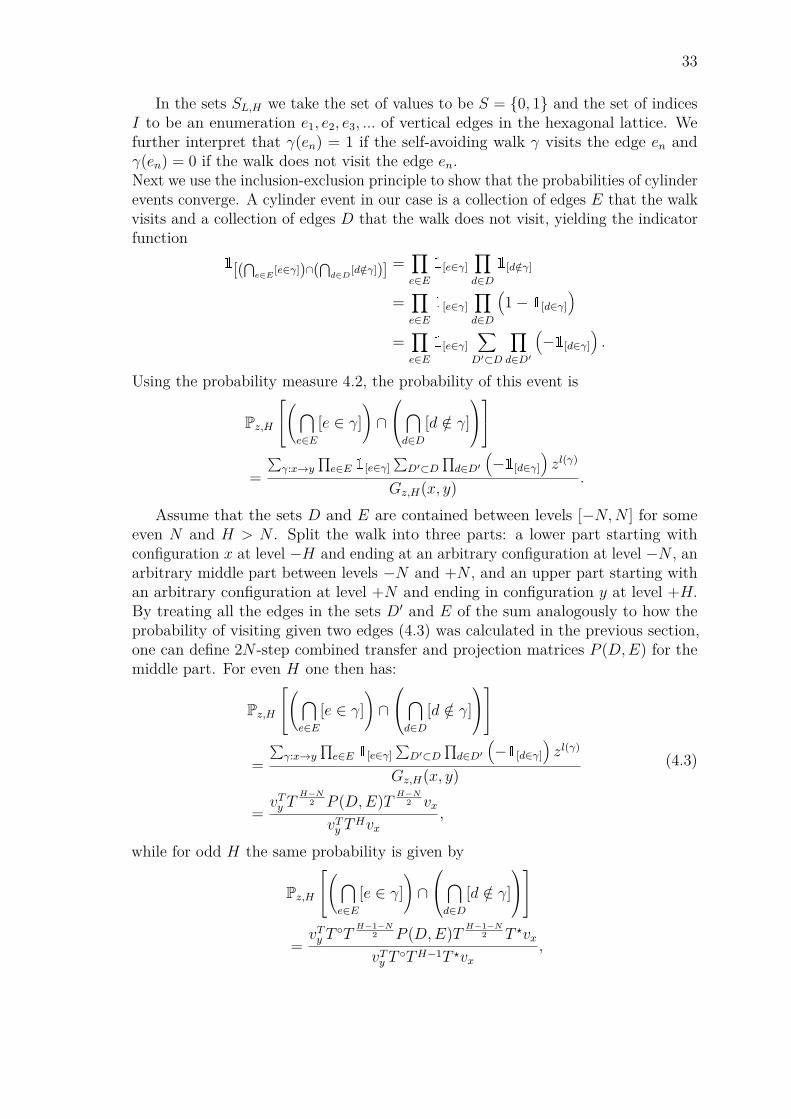
Figure 16: Transition from a configuration of no arcs to arbitrarily many arcs andback
where T ? again denotes the odd-to-even transfer matrix and T the even-to-oddtransfer matrix.
Proposition 4.18. In domains where the set of arc-thread configurations at levelh is the same as the one at level h + n for some n ∈ N and all h, all reachableconfigurations belong to the same communication class and the configurations areaperiodic. Therefore the Perron-Frobenius theorem applies to submatrices of reachableconfigurations of the corresponding n-step transfer matrices.
Proof. Let us start with a configuration of one thread and no arcs. To see thatall configurations belong to the same connection class, consider a transition to aconfiguration with m sets of arcs inside each other to added the right of the threadand n sets of arcs inside each other added to the left of the thread. To make thetransition to this system and back, we can make the walk traverse first through thearcs on the right, going each set from the outermost arc to the innermost arc andthen continuing to the next set. After all arcs on the right have been traversed,the walk goes straight to the left to the arc set closest to where the thread is andwhat happened on the right hand side is repeated. Finally the walk exits to thecenter, proving that also the transition back from the configuration with arcs to theconfiguration with no arcs is possible. This is shown in fig. 16. It is trivial that for aconfiguration with no arcs, the thread can stay where it was with a single transition,and the thread can be moved anywhere with a finite number of transitions, whichcompletes the proof.
In particular the proposition implies that there exists a triplet (λ,wT , v) suchthat
• λ is a unique positive eigenvalue of T
• v is a unique non-negative right eigenvector of T with positive entries vi forevery i corresponding to a reachable configuration αi.
35
• wT is a unique non-negative left eigenvector of T with positive entries wi forevery i corresponding to a reachable configuration αi.
• For every non-negative column vector u 6= 0 there are positive constants Au, Bu
such thatlimk→∞
T ku
λk= Auv, lim
k→∞
uTT k
λk= Buw
T .
Applying these identities to equation 4.3 for fixed D,E and any sequence of endpoints(xH , yH)H>N, we have
limH→∞
Pz,H
(⋂e∈E
[e ∈ γ])∩
⋂d∈D
[d /∈ γ]
= limH→∞
wTBλbH−N
2 cP (D,E)λbH−N2 cAv
wTBλbH−N
2 cTNλbH−N
2 cAv
= wTP (D,E)vwTλNv
This means that the probabilities of cylinder events converge as H tends to infinity,which in turn implies that there exists a limit measure Pz that the sequence (Pz,H)H∈Nconverges to.For the limit measure Pz we get the edge visiting probabilities by taking the limitand using properties of the matrix T for equations (4.3) and (4.3). Here we canwithout loss of generality assume that H is even. For the edge e = a+ ib
Pz[e ∈ γ]= lim
H→∞Pz,H [e ∈ γ]
= limH→∞
vTy TbH−b2 c(T )1[b odd]P (a)(T ?)1[b odd]T b
H+b2 cvx
vTy THvx
.
This is simplified similarly to the probability of a cylinder event, resulting in
Pz[e ∈ γ]
= limH→∞
vTy TbH−b2 c(T )1[b odd]P (a)(T ?)1[b odd]T b
H+b2 cvx
vTy TbH−b2 cT 1[b odd]T b
H+b2 cvx
= limH→∞
ABwTλbH−b
2 c(T )1[b odd]P (a)(T ?)1[b odd]λbH+b
2 cv
ABwλbH−b
2 cλ1[b odd]λbH+b
2 cv
= wT (T )1[b odd]P (a)(T ?)1[b odd]v
wλ1[y odd]v.
Likewise the limit of the probability 4.3 of visiting two edges
e1 = a1 + ib1, e2 = a2 + ib2
36
at heights b1 ≤ b2 can be calculatedPz[e1, e2 ∈ γ]= lim
H→∞Pz,H [e1, e2 ∈ γ]
= limH→∞
vTy TbH−b22 c(T )1[b2 odd]P (a2)(T ?)1[b2 odd]T b
b22 c−d
b12 e(T )1[b1 odd]P (a1)(T ?)1[b1 odd]T b
H+b12 cvx
vTy THvx
.
= wT (T )1[b2 odd]P (a2)(T ?)1[b2 odd]T bb22 c−d
b12 e(T )1[b1 odd]P (a1)(T ?)1[b1 odd]v
wTλ1[b1 odd]+1[b2 odd]+bb22 c−d
b12 ev
.
(4.4)
4.5 The Markov property of the limit measureNext we show that the limit measure Pz defines a Markovian process with respect tolevels. The probability measure Pz (respectively Pz,H) is a distribution on the set ofwalks γ. By proposition4.6 a walk γ can be characterized by the infinite (resp. finite)sequence of configurations (αh)h∈Z indexed by height. For a random self-avoidingwalk γ, the sequence (αh) can be thought of as a configuration-valued stochasticprocess indexed by h. This process turns out to be Markovian.Start with the two-edge visit probability (4.4) defined above, substitute b2 = b1 + 1and replace the projection matrices P (a1), P (a2) by matrices P (α), P (β) projectingonto configurations α and β, respectively. This renders the probability of the walkreaching configuration β at level h+ 1 and configuration α at level h to:Pz,H [γh+1 = β, γh = α]
=vTy T
bH−h−12 c(T )1[h+1 odd]P (β)(T ?)1[h+1 odd](T )1[h odd]P (α)(T ?)1[h odd]T b
H+h2 cvx
vTy THvx
.
Using the same technique on the single edge visit probability yields the probabilityof the walk reaching configuration α at level h.
Pz,H [γh = α] =vTy T
bH−h2 c(T )1[h odd]P (α)(T ?)1[h odd]T bH+h
2 cvx
vTy THvx
.
Combining these two, the conditional probability for the event γh+1 = β with thecondition γh = α is
Pz,H [γh+1 = β|γh = α] = Pz,H [γh+1 = β, γh = α]Pz,H [γh = α]
=vTy T
bH−h−12 c(T )1[h+1 odd]P (β)(T ?)1[h+1 odd](T )1[h odd]P (α)(T ?)1[h odd]T b
H+h2 cvx
vTy TbH−h2 c(T )1[h odd]P (α)(T ?)1[h odd]T b
H+h2 cvx
To simplify the equation, we will treat the cases h even, h odd separately. When his even
Pz,H [γh+1 = β|γh = α, h even]
=vTy T
H−h−22 T P (β)T ?P (α)T H+h
2 vx
vTy TH−h
2 P (α)T H+h2 vx
.

37
Taking the limit H →∞ yields
Pz[γh+1 = β|γh = α, h even] = wT P (β)T ?P (α)vwλP (α)v .
Doing the same calculations for odd h yields
Pz[γh+1 = β|γh = α, h odd] = wP (β)T P (α)T ?vwT P (α)T ?v .
In neither of these cases does the conditional probability depend on the trajectory ofthe walk below level h, thus we conclude that the limit measure Pz for infinitely longself-avoiding walks on the strip SL is Markovian with respect to the configurationsat integer levels. It should be noted however, that the measures Pz,H for walks onthe finite strip domains SL,H do not share this property.
38
5 Computations with the transfer matrixThe goal of this section is to provide computational support for the conjecturethat the scaling limit of the critical self-avoiding walk is conformally invariant. Weconsider the SAW in a vertical strip. Fixing the width of the strip and the fugacityz, we present a way to construct the sets of possible configurations CO, CE for bothdefinitions of SL and assemble the transfer matrices T , T ?. By taking the matrixproduct of these, we have the square matrix T , eigenvalues and eigenvectors ofwhich determine the limit measure PL. After computationally solving the largesteigenvalue and the associated eigenvectors of the matrix T , the idea is to compare theprobability of a self-avoiding walk in the infinite strip returning to the edge of stripwith the probability of the conformally invariant half-plane curve chordal SLE8/3returning to the real line. When the strip is conformally mapped to the half-planethe probabilities of the SAW and the SLE returning to the real line should convergeas the mesh size of the strip approaches zero.There are five steps to be done in this process:
• Constructing the sets of possible configurations CO, CE
• Assembling the transfer matrices T , T ?, T
• Solving the largest eigenvalue and corresponding left and right eigenvectors ofthe square matrix T
• Calculating the probabilities of a walk in the infinite strip returning to theright boundary of the strip
• Comparing these probabilities with the two-point function of chordal SLE8/3.
5.1 Constructing the sets of possible configurationsRecalling definition 4.5, the idea is to consider all ways to place the thread in thesystem of L edges. For all thread placements we want to calculate all possible waysto place arcs to the left of the edge and all ways to place arcs to the right of the edge.We then get the basis of arc-thread configurations by taking the union over all threadlocations for the cartesian product of the location of the thread, all ways to placearcs to the left of the thread and all ways to place arcs to the right of the thread .The task of constructing the basis for a level that is L− 1 hexagons, or L edges, widecan be reduced to
• Creating a function that calculates all possible ways fill an even number 2n ofedges [1, 2, . . . , 2n] with n arcs.
• Saving the full arc configurations on the interval [1, 2, . . . , 2n].
• Creating a function that returns all subsets with even number of members froma given interval
39
• Creating a function that replaces the indices [1, 2, . . . , 2n] of a precomputedfull arc configuration with the indices [i1, i2, . . . , i2n] of an arbitrary set of 2nedges
• Creating a function that places the thread in edge k in the system of l edgesindexed as 1, 2, . . . , L and calculates the set Lk of legitimate arc configurationsin the interval [1, . . . , k − 1] and the set Rk of legitimate arc configurations inthe interval [k + 1, . . . , L]
• Collecting the configurations associated to thread placement k by taking thecartesian product k × Lk ×Rk.
• Finally we get all configurations by looping k over 1, 2, ..., L and taking theunion
L⋃k=1k × Lk ×Rk.
cartesianProd[a_List, b_List] :=Map[a[[#[[1]]]], b[[#[[2]]]] &,Flatten[Table[i, j, i, 1, Length[a], j, 1, Length[b]], 1]];
As a preliminary function for the main loop we define a Cartesian product fortwo sets with lists of elements a and b as the collection of all pairs where first part ofthe pair comes from the first set, and the second part of the pair comes from thesecond set.
arcsList[0] = ;combineArcConfigs[p_, n_] :=
Map[Union[1, p, #] &,Map[Apply[Union, #] &,cartesianProd[arcsList[(p - 2)/2] + 1,arcsList[(2*n - p)/2] + p]]];
arcsList[n_Integer /; n > 0] :=Apply[Union, Map[combineArcConfigs[#, n] &, Range[2, 2*n, 2]]];
The function arcsList[n] gives all ways to fill edges [1, 2, . . . , 2n] with arcs.arcsList[0] is defined as the one-element set containing only the empty set. Forarguments n > 0, we use recursion. combineArcConfigs[p_ ,n_ ] is a functionthat gives union of the arc 1, p with the cartesian product of the possible ways tofill the interval [2, p− 1] with arcs and the possible ways to fill the interval [p+ 1, 2n]with arcs. Letting p run from 2 to 2n in steps of 2 and collecting the results, weget all ways to fill the the interval [1, 2n] with arcs. This is what the functionarcsList[n_Integer /; n > 0] does.
evenSubsets[a_List] :=Apply[Union, Map[Subsets[a, 2*#] &, Range[0, Length[a]/2]]];

40
The function evenSubsets does the second step in the algorithm of constructingthe basis, it gives all sublists of even parity for a list of edges.
confSubset[a_List] :=Module[conf = preCompArcs[[(Length[a]/2) + 1]], n,For[n = Length[a], n >= 1, n--, conf = conf /. n -> a[[n]]];conf];
The function confSubset does the third step in the algorithm. It takes in asargument a list i1, ..., i2m and starting from 2m replaces all instances of k by ik inthe set of precomputed full arc configurations for the interval 1, 2, ..., 2m. In otherwords it gives all ways to fill an arbitrary list of even parity with arcs.
Using functions evenSubsets and confSubset it is now possible to create thesets of admissible arc configurations Lk and Rk left and right to a thread placed inedge k. An example of the whole program to construct the basis is presented below.
basis[l_Integer, nl_Integer] :=Module[ basisv = ,(* l := number of edges*)(*nl := number of threads *)
preCompArcs =Table[arcsList[k], k, 0, Floor[(l - nl)/2]];(*Precompute and savefull arc configurations for the intervals [1,2m], m=0,1,2,...
l-nl is the largest possible length for the interval*)
grid = Range[l]; (* the set of edges 1,2,...,l*)
threadloc =Subsets[grid, nl]; (*all possible ways to place the nl thread(s)*)
For[i = 1, i <= Length[threadloc], i++,(* index the possible ways to place the thread(s) with i *)config[i] = ;(* config[i] := configurations associated to thread location i*)threadloc[[i]] = Union[0, threadloc[[i]], l + 1];
For[j = 1, j <= nl + 1, j++,
(*numerate the intervals between the threads by j*)
interval[i][j] =Range[threadloc[[i, j]] + 1, threadloc[[i, j + 1]] - 1];
(*Form the intervals*)
arcs[i][j] =Apply[Union, Map[confSubset[#] &, evenSubsets[interval[i][j]]]];
(*arcs[i][j] the arc configurations of the jth interval in the thread placement i*)
If[arcs[i][j] != && Length[config[i]] != 0,config[i] = cartesianProd[config[i], arcs[i][j]];]
If[Length[config[i]] == 0,config[i] = arcs[i][j];]
(*collect to config[i]:
41
all arc possibilities of the intervals j*)];
threadloc[[i]] = Most[Rest[threadloc[[i]]]];
config[i] = cartesianProd[threadloc[[i]], config[i]];
(*add the information about thread placement*)basisv = Union[basisv, config[i]](*add the configurations associated to the thread placement i to the union*)];
basisv];
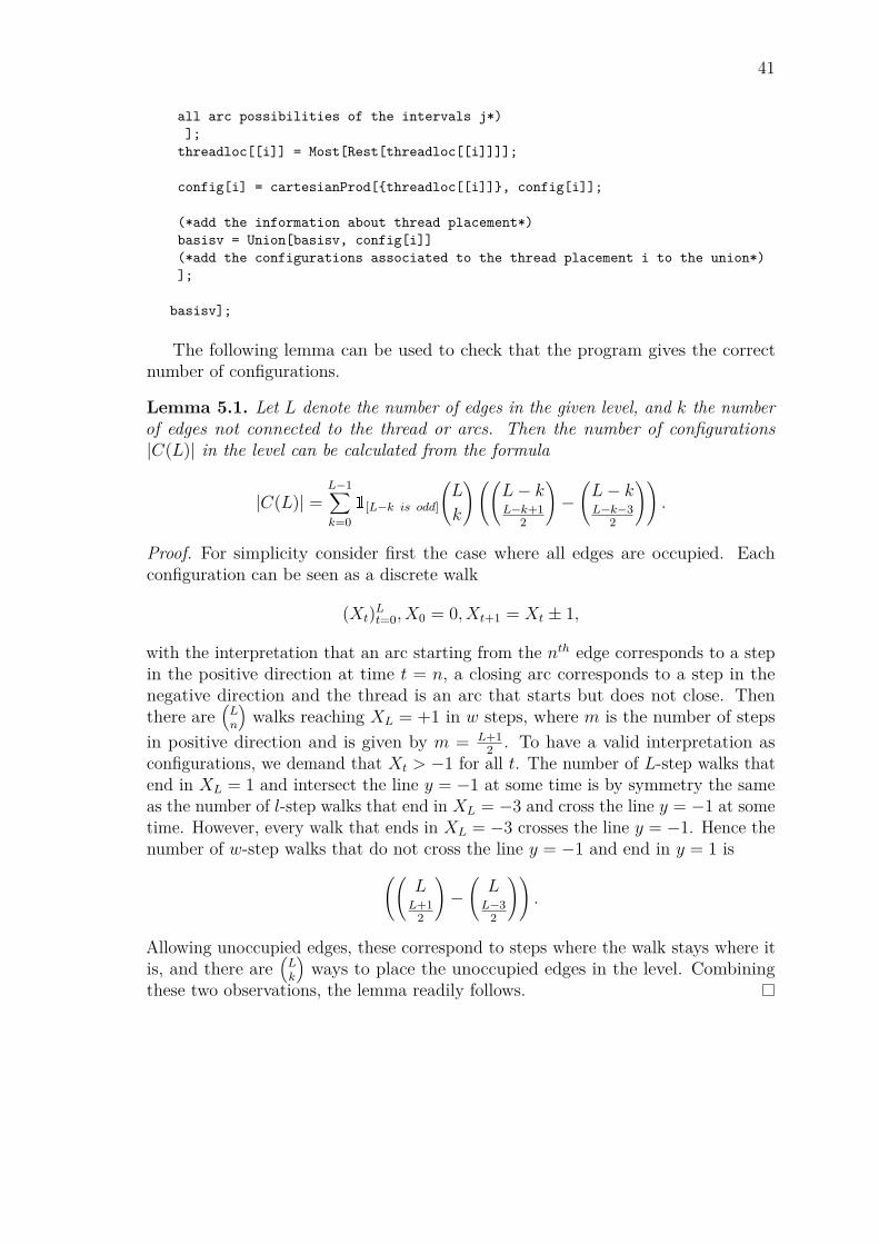
The following lemma can be used to check that the program gives the correctnumber of configurations.
Lemma 5.1. Let L denote the number of edges in the given level, and k the numberof edges not connected to the thread or arcs. Then the number of configurations|C(L)| in the level can be calculated from the formula
|C(L)| =L−1∑k=0
1[L−k is odd]
(L
k
)((L− kL−k+1
2
)−(L− kL−k−3
2
)).
Proof. For simplicity consider first the case where all edges are occupied. Eachconfiguration can be seen as a discrete walk
(Xt)Lt=0, X0 = 0, Xt+1 = Xt ± 1,
with the interpretation that an arc starting from the nth edge corresponds to a stepin the positive direction at time t = n, a closing arc corresponds to a step in thenegative direction and the thread is an arc that starts but does not close. Thenthere are
(Ln
)walks reaching XL = +1 in w steps, where m is the number of steps
in positive direction and is given by m = L+12 . To have a valid interpretation as
configurations, we demand that Xt > −1 for all t. The number of L-step walks thatend in XL = 1 and intersect the line y = −1 at some time is by symmetry the sameas the number of l-step walks that end in XL = −3 and cross the line y = −1 at sometime. However, every walk that ends in XL = −3 crosses the line y = −1. Hence thenumber of w-step walks that do not cross the line y = −1 and end in y = 1 is((
LL+1
2
)−(LL−3
2
)).
Allowing unoccupied edges, these correspond to steps where the walk stays where itis, and there are
(Lk
)ways to place the unoccupied edges in the level. Combining
these two observations, the lemma readily follows.
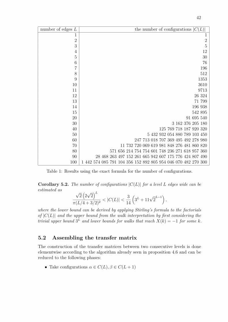
42
number of edges L the number of configurations |C(L)|1 12 23 54 125 306 767 1968 5129 135310 361011 971312 26 32413 71 79914 196 93815 542 89520 91 695 54030 3 162 376 205 18040 125 769 718 187 920 32050 5 432 932 054 880 789 103 45060 247 713 018 707 369 495 492 278 98070 11 732 720 069 619 981 848 276 481 860 82080 571 656 214 754 754 601 748 236 271 618 957 36090 28 468 263 497 152 261 665 942 607 175 776 424 807 490100 1 442 574 085 791 104 356 152 892 805 954 046 070 482 270 300
Table 1: Results using the exact formula for the number of configurations.
Corollary 5.2. The number of configurations |C(L)| for a level L edges wide can beestimated as √
2(2√
2)L
π(L/4 + 3/2)2 < |C(L)| < 314
(3L + 11
√2L−1
),
where the lower bound can be derived by applying Stirling’s formula to the factorialsof |C(L)| and the upper bound from the walk interpretation by first considering thetrivial upper bound 3L and lower bounds for walks that reach X(k) = −1 for some k.
5.2 Assembling the transfer matrixThe construction of the transfer matrices between two consecutive levels is doneelementwise according to the algorithm already seen in proposition 4.6 and can bereduced to the following phases:
• Take configurations α ∈ C(L), β ∈ C(L+ 1)

43
• Reindex the configuration of larger basis with the mapping x 7→ 2x− 1 andthe configuration of the smaller basis with the mapping x 7→ 2x.
• Take the union of the reindexed configurations, and form pairs such thatthe edge with the smallest coordinate in the union is paired with the secondsmallest, the third smallest with the fourth smallest etc. until all edges in theunion have been paired. These pairs have a direct interpretation as the set ofwalk segments that forms the part of the path the self-avoiding walk assumesbetween the configurations.
• Check the following conditions, and return 0 if any of them occur:
1. There is an upper configuration arc between the locations of the threads2. There is a walk segment from an end point of an arc of the upper configu-
ration to another arc of the upper configuration3. There is a walk segment from an end point of an arc of the upper configu-
ration to the thread of the upper configuration4. There is a closed system of arcs in the lower configurations that forms a
loop, i.e. there is an arc in the lower configuration such the left end of thearc starts a walk segment, the right end of the arc ends a walk segment
20 40 60 80 100 120 140
50
100
150
Figure 17: log |C(L)| plotted against L. The blue curve is the upper bound314
(3L + 11
√2L−1
)and the green curve is the lower bound
√2(2√
2)Lπ(L/4+3/2)2 .
44
and there is no arc in the upper configuration between the end points ofthe arc.
• If none of the above conditions are met, calculate the total length of the walksegments connecting the two configurations, i.e. the number of diagonal edgesin the walk segments plus the total number of edges in the configurations times1/2 one half corresponding to the half-edge steps in the walk segments.
• Returning the total length l(α→ β) and saving it in the matrix element T ?(β,α).
• Loop through all of C(L) × C(L + 1) to construct the complete matrix T ?.Similarly loop through all of C(L+ 1)× C(L) to construct the matrix T .
The number of configurations C(L) × C(L + 1) grows exponentially fast bycorollary 5.2, and saving the matrices became too memory-intensive for my hardwarewhen L reached the value 11. Checking the conditions 2, 3 and 4 above is slow, so itis more efficient to first drop out elements of the matrix that satisfy the condition 1.
width = 10;longb = 2*basis[width + 1, 1] - 1;shortb = 2*basis[width, 1];
First fix the width L and calculate the two bases C(L) and C(L+ 1), map thenarrower basis C(L) to a set of even indices and the wider basis C(L+ 1) to a set ofodd indices using the existing main loop basis of the previous section.
indexNW = Block[indices,indices = ;For[j = 1, j <= width + 1, j++,jpos = Flatten[Position[longb, 2*j - 1][[All, 1]]];For[i = 1, i <= width, i++,ijfree = ;Do[If[IntersectingQ[Flatten[longb[[jpos[[k]], 2]]],
Range[Min[2*i + 1, 2*j + 1], Max[2*i - 1, 2*j - 3], 2]] ==False, ijfree = Union[ijfree, jpos[[k]]]],k, 1, Length[jpos]];
indices =Union[indices,cartesianProd[ijfree[[Range[1, Length[ijfree]]]],Flatten[Position[shortb, 2*i][[All, 1]]]]];
];];
indices]; // Timing
Run through all thread positions jpos in the wider basis of configurations C(L+1)and for all configurations βj associated so jpos = j check all thread locations i ofthe narrower basis C(L). Collect to list ijfree all configurations in the upperconfiguration with nothing between i and j and take the cartesian product of ijfreeand the list of configurations αi in C(L) with the thread location i. This yields the
45
list of pairs of configurations (β, α) ∈ C(L + 1) × C(L) for which the transitionα→ β is plausible according to the first condition. The naming indexNW comes fromthe transition Narrow to Wide.
zcrit = N[1/Sqrt[2 + Sqrt[2]], 10];pairDiff[a_List] := Range[a[[1]], a[[2]]];
Use a ten-decimal numerical approximation for the critical constant zc = 1µ. Define
the function pairDiff as the difference of the two members of the pair.
cNW = Function[wind, nind,(*The transfer matrix element from the shorter basis to the longer one:a\[Rule]b corresponds to element (b,a)*)Block[longvect = Flatten[longb[[wind]]],
shortvect = Flatten[shortb[[nind]]], element,upp = Sort[longvect];path = Sort[Join[longvect, shortvect]];(*The start and end of the path*)pathden =Transpose[path[[Range[1, Length[path], 2]]],
path[[Range[2, Length[path], 2]]]];
The building of a transfer matrix NW from the narrow basis C(L) to the widebasis C(L + 1) begins with the initiation. wind is the configuration β ∈ C(L + 1)and nind is the configuration α ∈ C(L). The variables longvect associated to windand shortvect associated to nind keep track of occupied edges but nothing else.The union of shortvect and longvect is named path and the variable path has theinformation of the canonical way to connect the two walks with walk segments. Thevariable pathden is a list of the end points of these walk segments.
(*Checks that the upper conf. thread is notconnected to an upper conf. arc*)(*upper conf. arcs*)upc = longvect[[Range[2, Length[longvect]]]];longden =Transpose[upc[[Range[1, Length[upc], 2]]],
upc[[Range[2, Length[upc], 2]]]];overden = Complement[posProd[upp, upp], longden];(*Checks that the upper conf. arcs are not connected to each other*)
If[IntersectingQ[pathden, overden], element = 0. Break];
The variable upc is a list of edges occupied by the upper configuration arcs.longden is a list of the upper configuration arcs. overden is a list of all ways to formwalk segments between the edges of upc that are not arcs in the upper configuration.If some of the walk segments in overden is in the set pathden, the configurationscannot be joined and the program returns 0. This amounts to checking the conditions2 and 3.
46
(*The lower conf. arcs*)lowc = shortvect[[Range[2, Length[shortvect]]]];shoden =Transpose[lowc[[Range[1, Length[lowc], 2]]],
lowc[[Range[2, Length[lowc], 2]]]];
rottenarcs =Intersection[posProd[path[[Range[1, Length[path], 2]]],path[[Range[2, Length[path], 2]]]], shoden];
The variable lowc gives the edges occupied by the lower configuration arcs, whileshoden gives the arcs themselves. The variable rottenarcs gives the intersection ofthe lower configuration arcs with pairs formed by combining left endpoints of thewalk segments with the right endpoints of the walk segments, i.e. it gives the lowerconfiguration arcs whose left end is the left end of a walk segment and right end theright end of a walk segment. Every such arc must have an upper configuration arc inbetween its end points.
If[ rottenarcs == ||FreeQ[Map[IntersectingQ[pairDiff[#], upc] &, rottenarcs], False],
element =zcrit^(Length[path]/2 +
Total[path[[Range[2, Length[path], 2]]] -path[[Range[1, Length[path], 2]]]]), element = 0.
](*return z^length of the walk segments if the walk segments are OK, otherwise 0*)
]];
The final part of the code tests condition 4 and returns the combined lengthof the legitimate walk segments if none of the conditions are met. By running thesame process with every index in indexNW we have the transfer matrix from thenarrow basis to the wide basis. The program assembling the transfer matrix from thewide basis to the narrow has the same phases, with only minor changes in definingvariables.
Parallelize[nw1 = cNW[#[[1]], #[[2]]] & /@
indexNW[[1 ;; Floor[Length[indexNW]/4]]];nw2 = cNW[#[[1]], #[[2]]] & /@
indexNW[[Floor[Length[indexNW]/4] + 1 ;; Floor[Length[indexNW]/2]]];
nw3 = cNW[#[[1]], #[[2]]] & /@indexNW[[
47
Floor[Length[indexNW]/2] + 1 ;; Floor[3*Length[indexNW]/4]]];nw4 = cNW[#[[1]], #[[2]]] & /@
indexNW[[Floor[3*Length[indexNW]/4] + 1 ;; Length[indexNW]]];, Method -> "CoarsestGrained"]; // AbsoluteTiming
nwval = Catenate[nw1, nw2, nw3, nw4]; // Timing
nw = SparseArray[indexNW -> nwval];
Export["nw10.mat", nw]; // Timing
To reduce computation time, the matrix elements of viable indices are calculatedin four parts and then catenated together. The resulting matrix is not too sparse,which makes saving the transfer matrices for large widths problematic.
With the program code we are able to calculate the transfer matrices betweenconsecutive layers of the hexagonal lattice for SAWs of different values of z.
5.3 Computational resultsThe theory developed in previous sections for a self-avoiding walk in vertical stripsdoes not depend on the scale or location of the strip. Thus we can fix the left andright boundaries of the strips SL to be 0 and π, while keeping the lattice such thatthe real line is at the center of a layer. We get finer and finer approximations of avertical strip in the complex plane by increasing the number of edges L in a layer.In particular in the approximation SL the mesh size δ equals π
L−1 . As we increase Lwe get closer to the possible scaling limit of the SAW. The following conjecture isour main tool in comparing the SAW with its conjectured scaling limit.
Conjecture 5.3. [JJK15] Consider a simply connected domain Ω ( C and let a, bbe two points on the boundary ∂Ω. Furthermore assume that there are sections of theboundary perpendicular to either coordinate axis with points c1, c2, . . . , cn on thesesections. Approximate the set Ω and the points a, b according to definition 2.7 withthe triplet (Ωδ, aδ, bδ) and let Pzc,Ωδ,a,b be the law of self-avoiding walks on the set Ωδ.Denote by cδk, k = 1, 2 . . . , n the edge on Ωδ closest to the boundary point ck. See alsofig. 18. If the scaling limit of the critical self-avoiding walk exists and is conformallyinvariant, by theorem 2.11 it must be the chordal Schramm-Löwner evolution SLE8/3.Associating the self-avoiding walk with chordal SLEκ yields the following estimate:
1δnh
Pzc,Ωδ,a,b[γ visits cδ1, cδ2, . . . , cδn
]−−→δ→0
ζΩ(a, b, c1, . . . , cn), (5.1)

48
δ
b
a
c1
c2
c3
...
...
...
. . . . . . . . . cn−1cn
Figure 18: An example of a simply connected domain Ω, its lattice approximationΩδ and the set of edges cδ1, . . . , cδn (red line segments) approximating boundary pointsc1, . . . , cn on parts of the boundary ∂Ω perpendicular to the coordinate axes.
whereζΩ(a, b, c1, . . . , cn) = C
n∏j=1|g′(cj)|hζ(n)(g(c1), g(c2), . . . g(cn)),
g : Ω→ H is a conformal mapping onto the uppper halfplane H with g(a) = 0,g(b) =∞, C is a constant dependent on the choice of the lattice and the approximationand ζ(n) is an explicit function for SLE boundary visit amplitudes, universal for alllattice approximations of Ω by the theory of renormalization groups. When n = 2and 0 < g(c1) < g(c2), we have
ζ(2)(g(c1), g(c2)) = |g(c1)|1−8/κ|g(c2)|1−8/κ2F1(4/κ, κ− 8
κ; 8κ
; g(c2)− g(c1)g(c2) ).
The constant κ and the exponent h = 88−κ are determined by the chordal SLEκ that
the self-avoiding walk is conjectured to converge to, namely SLE8/3, to be κ = 8/3,h = 2.
The idea for producing computational support for the conjecture 2.10 using ourprevious results and conjecture 5.3 is as follows:
49
• Choose the open strip S = z ∈ C | 0 < Re(z) < π as the simply connecteddomain Ω.
• Translate and scale the infinite strip SL of section 4.1 of the hexagonal latticeso that the real part of the leftmost edge on the real line is 0 and the real partof rightmost edge on the real line is π. This makes the width of the hexagonsequal π
L−1 , which implies that the height difference between two consecutivelevels is
√3π
L−1 . In other words for δ = πL−1 the hexagonal lattice strip SL equals
Ωδ in the conjecture 5.3.
• Choose the boundary points to be a = −i∞ and b = +i∞. The conditionsg(a) = 0, g(b) = ∞ and the choice g(π) = 1 then determine the conformalmapping g from domain S to the half-plane H = z ∈ C | Im(z) ≥ 0 to be
g(z) = ei(π−z), g′(x+ iy) = ieye−ix.
• Consider the points cL:k := π + i√
3πkL−1 with imaginary coordinate on the (2k)th
level of the set SL and real coordinate on the right boundary of the strip S.
• By section 4.4 the probability measure PL = Pzc,SL,−i∞,+i∞ for infinitely longSAWs exists and we can explicitly calculate the probabilities of visiting twopoints:
PL[γ visits cδL;0, cδL;k] = wTP (π)T kP (π)v
λkwTv.
• When n = 2, c1 = cL;0 and c2 = cL;k the right-hand side of equation (5.1) isreduced to
ζS(−i∞,+i∞, cL;0 = π, cL;k)
= C|g′(π)|2|g′(cL;k)|2|g(π)|−2|g(cL;k)− g(π)|−22F1(3/2,−2; 3; g(cL;k)− g(π)
g(cL;k))
= C|g′(cL;k)|2|g(cL;k)− 1|−22F1(3/2,−2; 3; g(cL;k)− 1
g(cL;k))
• Finally we have that if conjecture 5.3 holds
(L− 1)4PL[γ visits cδL;0, cδL;k]
|g′(cL;k)|2−−−→L→∞
C|g(cL;k)−1|−22F1(3/2,−2; 3; g(cL;k)− 1
g(cL;k)).
We test this conjecture by plotting the points(g(cL;k),
(L− 1)4PL[γ visits cδL;0, cδL;k]
|g′(cL;k)|2
)(5.2)
against the graph of the function C|x−1|−22F1(3/2,−2; 3; x−1
x) for various k, L
with C chosen to minimize the least squares distance between the graph andthe points.
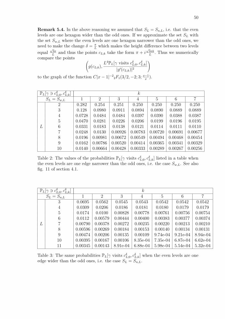
50
Remark 5.4. In the above reasoning we assumed that SL = Sn,L, i.e. that the evenlevels are one hexagon wider than the odd ones. If we approximate the set SL withthe set Sw,L where the even levels are one hexagon narrower than the odd ones, weneed to make the change δ = π
Lwhich makes the height difference between two levels
equal√
3πL
and thus the points cL;k take the form π + i√
3πkL. Thus we numerically
compare the points (g(cL;k),
L4PL[γ visits cδL;0, cδL;k]
|g′(cL;k)|2
)to the graph of the function C|x− 1|−2
2F1(3/2,−2; 3; x−1x
).
PL[γ 3 cδL;0, cδL;k] k
SL = Sw,L 1 2 3 4 5 6 7
L
2 0.282 0.254 0.251 0.250 0.250 0.250 0.2503 0.128 0.0980 0.0911 0.0894 0.0890 0.0889 0.08894 0.0728 0.0484 0.0484 0.0397 0.0390 0.0388 0.03875 0.0470 0.0281 0.0226 0.0206 0.0199 0.0196 0.01956 0.0331 0.0183 0.0138 0.0121 0.0114 0.0111 0.01107 0.0248 0.0130 0.00926 0.00783 0.00720 0.00691 0.006778 0.0196 0.00981 0.00672 0.00549 0.00494 0.00468 0.004549 0.0162 0.00786 0.00520 0.00414 0.00365 0.00341 0.0032910 0.0140 0.00664 0.00428 0.00333 0.00289 0.00267 0.00256
Table 2: The values of the probabilities PL[γ visits cδL;0, cδL;k] listed in a table when
the even levels are one edge narrower than the odd ones, i.e. the case Sw,L. See alsofig. 11 of section 4.1.
PL[γ 3 cδL;0, cδL;k] k
SL = Sn,L 1 2 3 4 5 6 7
L
3 0.0695 0.0562 0.0545 0.0543 0.0542 0.0542 0.05424 0.0309 0.0206 0.0186 0.0181 0.0180 0.0179 0.01795 0.0174 0.0100 0.00828 0.00778 0.00761 0.00756 0.007546 0.0112 0.00579 0.00444 0.00400 0.00383 0.00377 0.003747 0.00790 0.00378 0.00272 0.00235 0.00220 0.00213 0.002108 0.00596 0.00269 0.00184 0.00153 0.00140 0.00134 0.001319 0.00474 0.00206 0.00135 0.00109 9.74e-04 9.21e-04 8.94e-0410 0.00395 0.00167 0.00106 8.35e-04 7.35e-04 6.87e-04 6.62e-0411 0.00345 0.00143 8.91e-04 6.88e-04 5.98e-04 5.54e-04 5.32e-04
Table 3: The same probabilities PL[γ visits cδL;0, cδL;k] when the even levels are one
edge wider than the odd ones, i.e. the case SL = Sn,L.
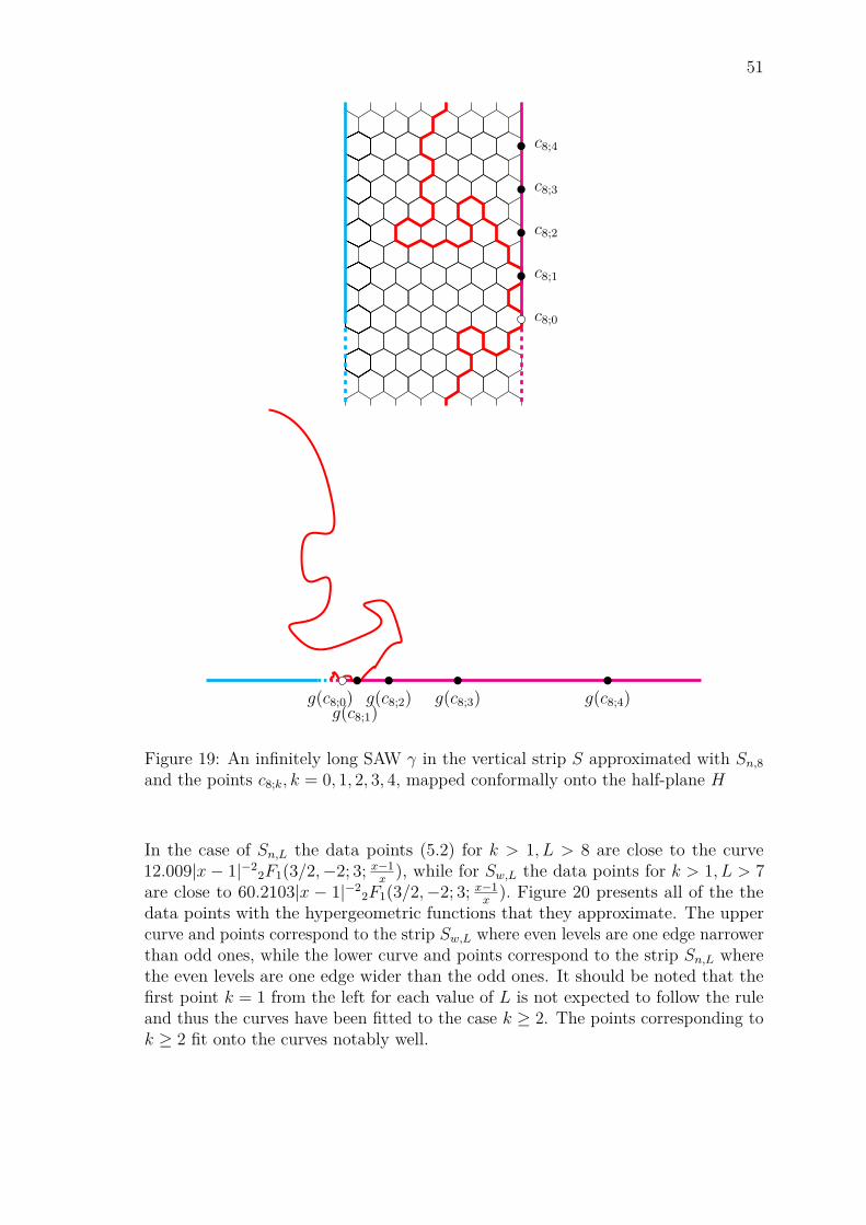
51
c8;1
c8;2
c8;3
c8;4
c8;0
g(c8;0)g(c8;1)
g(c8;2) g(c8;3) g(c8;4)
Figure 19: An infinitely long SAW γ in the vertical strip S approximated with Sn,8and the points c8;k, k = 0, 1, 2, 3, 4, mapped conformally onto the half-plane H
In the case of Sn,L the data points (5.2) for k > 1, L > 8 are close to the curve12.009|x− 1|−2
2F1(3/2,−2; 3; x−1x
), while for Sw,L the data points for k > 1, L > 7are close to 60.2103|x − 1|−2
2F1(3/2,−2; 3; x−1x
). Figure 20 presents all of the thedata points with the hypergeometric functions that they approximate. The uppercurve and points correspond to the strip Sw,L where even levels are one edge narrowerthan odd ones, while the lower curve and points correspond to the strip Sn,L wherethe even levels are one edge wider than the odd ones. It should be noted that thefirst point k = 1 from the left for each value of L is not expected to follow the ruleand thus the curves have been fitted to the case k ≥ 2. The points corresponding tok ≥ 2 fit onto the curves notably well.

52
2 4 6 8 10 12
0.01
0.10
1
10
100
Figure 20: Hypergeometric curves |x − 1|−22F1(3/2,−2; 3; x−1
x) fitted against the
data points g(cL;k),(L− 1)4PL
[γ visits cδL;0, c
δL;k
]|g′(cL;k)|2
for Sn,L,g(cL;k),
L4PL[γ visits cδL;0, c
δL;k
]|g′(cL;k)|2
for Sw,L.
Color coding: L = 11 as black, L = 10 as blue, L = 9 as red, L = 8 as green, L = 7as orange.
The data provides numerical support for conjecture 5.3 that has been derivedfrom the assumption that the scaling limit of the self-avoiding walk is the Schramm-Löwner Evolution SLE8/3. Hence we also provide further evidence for the conformalinvariance conjecture 2.10.
53
References[AJ90] E. Alm and S. Janson. Random self-avoiding walks on one-dimensional
lattices. Communications in Statistics. Stochastic Models., 6(2):169–212,1990.
[DCKY14] H. Duminil-Copin, G. Kozma, and A. Yadin. Supercritical self-avoidingwalks are space-filling. Ann. Inst. Henri Poincaré., 50(2):315–326, 2014.
[DCS12] H. Duminil-Copin and S. Smirnov. The connective constant of thehoneycomb lattice equals
√2 +√
2. Ann. Math., 175(3):1653–1665,2012.
[Flo53] P. Flory. Principles of Polymer Chemistry. Cornell University Press.,1953.
[Iof98] D. Ioffe. Ornstein-Zernike behaviour and analyticity of shapes for self-avoiding walks on Zd. Markov Process. Related Fields, 4(3):323–350,1998.
[JJK15] N. Jokela, M. Järvinen, and K. Kytölä. SLE boundary visits. Ann. Inst.Henri Poincaré., pages 1–68, 2015.
[LSW04a] G. Lawler, O. Schramm, and W. Werner. Conformal invariance of planarloop-erased random walks and uniform spanning trees. Ann. Probab.,32(1B):939–995, 2004.
[LSW04b] G. Lawler, O. Schramm, and W. Werner. On the scaling limit of planarself-avoiding walk. In Proc. Sympos. Pure Math., volume 72 of Fractalgeometry and applications: a jubilee of Benoît Mandelbrot, Part 2, pages339–364. Amer. Math. Soc., 2004.
[MS93] N. Madras and G. Slade. The Self-Avoiding Walk. Birkhäuser, Boston.,1993.
[Nie82] B. Nienhuis. Exact critical point and critical exponents of O(n) modelsin two dimensions. Phys. Rev. Lett., 49(15):1062–1065, 1982.
[Shi95] A. Shirayev. Probability. Number 95 in Graduate Texts in Mathematics.Springer-Verlag, New York., 2nd edition, 1995.
[Sla06] G. Slade. The Lace Expansion and its Applications. Springer-VerlagBerlin Heidelberg., 2006.
[Smi01] S. Smirnov. Critical percolation in the plane. Comptes Rendus del’Académie des Sciences., 333(3):239–244, 2001.
54
[Smi06] S. Smirnov. Towards conformal invariance of 2D lattice models. InM. Sanz-Solé, editor, Proceedings of the international congress of mathe-maticians (ICM), volume II: Invited lectures, pages 1421–1451. Zürich:European Mathematical Society (EMS), August 2006.