Embed Size (px)
Citation preview
DeepWeibull: a deep learning approach toparametric survival analysis
by
Matthew Pawley
M4R: Advanced Research Project in MathematicsMSci MathematicsImperial College LondonJune 2020Supervisor: Professor Axel Gandy


Plagiarism statement
This is my own work except where otherwise stated.
Matthew Pawley, June 2020
i
Abstract
Survival analysis is a widely applicable field of statistics concerned with the modellingthe time until an event occurs. A key objective of survival analysis is to learn the rela-tionship between covariates and the distribution of survival times. There are existingmethods which use machine learning to tackle the problem. Some approaches tend toimpose very restrictive and unrealistic assumptions on both the form of the underlyingstochastic process and on the relationship between the covariates and the parametersof the process. Others are more flexible and make no such assumptions, which meansthey are unreliable when there is little training data available, which is common insurvival analysis. We propose a new model, DeepWeibull, which uses a deep neuralnetwork to learn the parameters of a Weibull distribution given a set of covariates.This approach combines the capability of neural networks to learn complex covariate-parameter relationships with the benefits of a Weibull parametric model: simplicity,flexibility, interpretability and reliability when sample sizes are small. Tests conductedon a range of simulated and real-world datasets demonstrate that DeepWeibull achievescomparable results with existing models and performs strongly when training data isscarce.
ii

Acknowledgements
With many thanks to my supervisor, Prof. Axel Gandy, for his help during this projectand advice about academia more generally and to my tutor, Prof. Alastair Young, forhis support throughout my time at Imperial.
iii
Contents
1 Introduction 1
1.1 Introduction . . . . . . . . . . . . . . . . . . . . . . . . . . . . . . . . . . 1
1.2 Thesis outline . . . . . . . . . . . . . . . . . . . . . . . . . . . . . . . . . 2
2 Survival analysis 3
2.1 Basic concepts . . . . . . . . . . . . . . . . . . . . . . . . . . . . . . . . 3
2.1.1 What is survival analysis? . . . . . . . . . . . . . . . . . . . . . . 3
2.1.2 Framework, censoring and notation . . . . . . . . . . . . . . . . . 4
2.1.3 Likelihood for censored data . . . . . . . . . . . . . . . . . . . . . 4
2.2 Parametric models . . . . . . . . . . . . . . . . . . . . . . . . . . . . . . 6
2.2.1 Exponential distribution . . . . . . . . . . . . . . . . . . . . . . . 6
2.2.2 Weibull distribution . . . . . . . . . . . . . . . . . . . . . . . . . 6
2.3 Performance metrics . . . . . . . . . . . . . . . . . . . . . . . . . . . . . 10
2.3.1 Discrimination and calibration . . . . . . . . . . . . . . . . . . . 10
2.3.2 Time-dependent concordance index . . . . . . . . . . . . . . . . . 11
2.3.3 Integrated Brier score . . . . . . . . . . . . . . . . . . . . . . . . 13
3 Neural networks 15
3.1 Basic concepts . . . . . . . . . . . . . . . . . . . . . . . . . . . . . . . . 15
3.1.1 Activation functions . . . . . . . . . . . . . . . . . . . . . . . . . 15
3.1.2 Loss functions . . . . . . . . . . . . . . . . . . . . . . . . . . . . 16
3.1.3 Training and testing . . . . . . . . . . . . . . . . . . . . . . . . . 17
4 Survey: neural networks in survival analysis 18
4.1 Cox model approaches . . . . . . . . . . . . . . . . . . . . . . . . . . . . 18
4.1.1 Cox proportional hazards model . . . . . . . . . . . . . . . . . . 18
4.1.2 The Faraggi-Simon model . . . . . . . . . . . . . . . . . . . . . . 19
4.1.3 DeepSurv . . . . . . . . . . . . . . . . . . . . . . . . . . . . . . . 20
4.1.4 Discussion . . . . . . . . . . . . . . . . . . . . . . . . . . . . . . . 20
4.2 Classification approaches . . . . . . . . . . . . . . . . . . . . . . . . . . . 20
4.2.1 Framework . . . . . . . . . . . . . . . . . . . . . . . . . . . . . . 20
4.2.2 Liesøl model . . . . . . . . . . . . . . . . . . . . . . . . . . . . . 21
4.2.3 Partial logistic regression models with ANN (PLANN) . . . . . . 21
4.2.4 Discussion . . . . . . . . . . . . . . . . . . . . . . . . . . . . . . . 22
4.3 DeepHit . . . . . . . . . . . . . . . . . . . . . . . . . . . . . . . . . . . . 22
4.3.1 Framework and notation . . . . . . . . . . . . . . . . . . . . . . . 22
4.3.2 Network configuration . . . . . . . . . . . . . . . . . . . . . . . . 23
4.3.3 Loss function . . . . . . . . . . . . . . . . . . . . . . . . . . . . . 24
iv
CONTENTS v
4.3.4 Training the neural network . . . . . . . . . . . . . . . . . . . . . 244.3.5 Results . . . . . . . . . . . . . . . . . . . . . . . . . . . . . . . . 254.3.6 Discussion . . . . . . . . . . . . . . . . . . . . . . . . . . . . . . . 25
5 Proposed model 275.1 Model description . . . . . . . . . . . . . . . . . . . . . . . . . . . . . . . 27
5.1.1 Framework and notation . . . . . . . . . . . . . . . . . . . . . . . 275.1.2 Network configuration . . . . . . . . . . . . . . . . . . . . . . . . 27
5.2 Loss function . . . . . . . . . . . . . . . . . . . . . . . . . . . . . . . . . 285.2.1 The loss function . . . . . . . . . . . . . . . . . . . . . . . . . . . 285.2.2 Unique global optimum . . . . . . . . . . . . . . . . . . . . . . . 285.2.3 Numerical instability for highly censored data . . . . . . . . . . . 295.2.4 Regularisation . . . . . . . . . . . . . . . . . . . . . . . . . . . . 29
5.3 Discussion . . . . . . . . . . . . . . . . . . . . . . . . . . . . . . . . . . . 29
6 Weibull data experiments 316.1 Weibull regression model . . . . . . . . . . . . . . . . . . . . . . . . . . . 31
6.1.1 The Gumbel distribution . . . . . . . . . . . . . . . . . . . . . . 316.1.2 RegressionWeibull . . . . . . . . . . . . . . . . . . . . . . . . . . 32
6.2 Simulated datasets . . . . . . . . . . . . . . . . . . . . . . . . . . . . . . 326.2.1 Description . . . . . . . . . . . . . . . . . . . . . . . . . . . . . . 326.2.2 Simulation methodology . . . . . . . . . . . . . . . . . . . . . . . 336.2.3 Oracle performance metrics . . . . . . . . . . . . . . . . . . . . . 34
6.3 Results . . . . . . . . . . . . . . . . . . . . . . . . . . . . . . . . . . . . . 356.3.1 Linear Weibull . . . . . . . . . . . . . . . . . . . . . . . . . . . . 356.3.2 Non-linear Weibull . . . . . . . . . . . . . . . . . . . . . . . . . . 376.3.3 Conclusions . . . . . . . . . . . . . . . . . . . . . . . . . . . . . . 38
7 Real-world data experiments 407.1 Datasets . . . . . . . . . . . . . . . . . . . . . . . . . . . . . . . . . . . . 40
7.1.1 Molecular Taxonomy of Breast Cancer International Consortium(METABRIC) . . . . . . . . . . . . . . . . . . . . . . . . . . . . 40
7.1.2 Study to Understand Prognoses Preferences Outcomes and Risksof Treatment (SUPPORT) . . . . . . . . . . . . . . . . . . . . . . 40
7.2 Results . . . . . . . . . . . . . . . . . . . . . . . . . . . . . . . . . . . . . 417.2.1 METABRIC . . . . . . . . . . . . . . . . . . . . . . . . . . . . . 417.2.2 SUPPORT . . . . . . . . . . . . . . . . . . . . . . . . . . . . . . 437.2.3 Conclusions . . . . . . . . . . . . . . . . . . . . . . . . . . . . . . 43
8 Discussion 468.1 Future work . . . . . . . . . . . . . . . . . . . . . . . . . . . . . . . . . . 468.2 Ethical considerations . . . . . . . . . . . . . . . . . . . . . . . . . . . . 478.3 Summary and conclusions . . . . . . . . . . . . . . . . . . . . . . . . . . 47
A Weibull data experiments: full results 53
B Real-world data experiments: full results 56
Chapter 1
Introduction
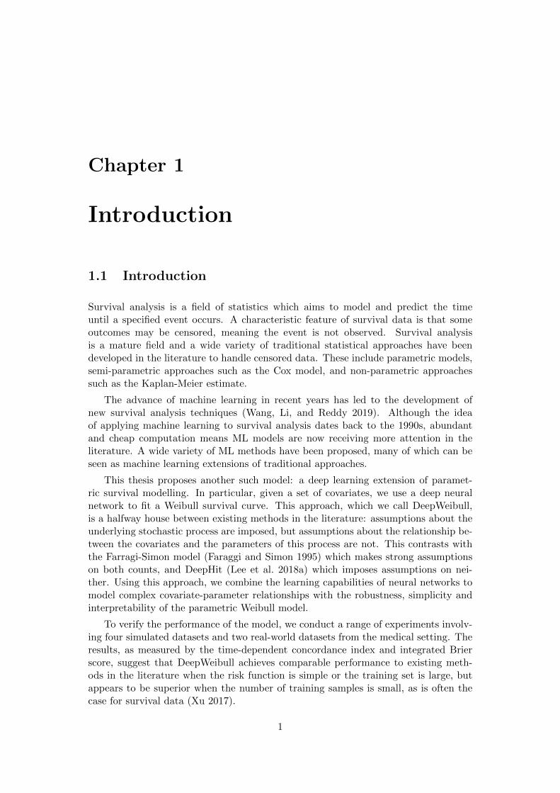
1.1 Introduction
Survival analysis is a field of statistics which aims to model and predict the timeuntil a specified event occurs. A characteristic feature of survival data is that someoutcomes may be censored, meaning the event is not observed. Survival analysisis a mature field and a wide variety of traditional statistical approaches have beendeveloped in the literature to handle censored data. These include parametric models,semi-parametric approaches such as the Cox model, and non-parametric approachessuch as the Kaplan-Meier estimate.
The advance of machine learning in recent years has led to the development ofnew survival analysis techniques (Wang, Li, and Reddy 2019). Although the ideaof applying machine learning to survival analysis dates back to the 1990s, abundantand cheap computation means ML models are now receiving more attention in theliterature. A wide variety of ML methods have been proposed, many of which can beseen as machine learning extensions of traditional approaches.
This thesis proposes another such model: a deep learning extension of paramet-ric survival modelling. In particular, given a set of covariates, we use a deep neuralnetwork to fit a Weibull survival curve. This approach, which we call DeepWeibull,is a halfway house between existing methods in the literature: assumptions about theunderlying stochastic process are imposed, but assumptions about the relationship be-tween the covariates and the parameters of this process are not. This contrasts withthe Farragi-Simon model (Faraggi and Simon 1995) which makes strong assumptionson both counts, and DeepHit (Lee et al. 2018a) which imposes assumptions on nei-ther. Using this approach, we combine the learning capabilities of neural networks tomodel complex covariate-parameter relationships with the robustness, simplicity andinterpretability of the parametric Weibull model.
To verify the performance of the model, we conduct a range of experiments involv-ing four simulated datasets and two real-world datasets from the medical setting. Theresults, as measured by the time-dependent concordance index and integrated Brierscore, suggest that DeepWeibull achieves comparable performance to existing meth-ods in the literature when the risk function is simple or the training set is large, butappears to be superior when the number of training samples is small, as is often thecase for survival data (Xu 2017).
1
2 CHAPTER 1. INTRODUCTION
1.2 Thesis outline
This thesis broadly consists of three sections: the theoretical background underpinningsurvival analysis and neural networks; the application of this theory to develop theproposed model, and experiments to test and compare the performance of the proposedmodel with alternative approaches.
Chapter 2 develops the necessary mathematics relating to survival analysis that willbe used later in the thesis. Section 3.1 develops the framework, notation and presentsthe likelihood for censored data. We show how this can be used to develop parametricsurvival models (Section 2.2) with a particular focus on the Weibull distribution andits properties. The performance metrics that will be used to test the models areintroduced in Section 2.3.
Chapter 3 provides a brief introduction to the topic of neural networks. An in-depth review of this field is beyond the scope of this thesis, but we will review activationfunctions (Section 3.1.1), loss functions (Section 3.1.2) and validation methods (Section3.1.3). For a more detailed introduction to the area, we refer to Hastie, Tibshirani,and Friedman (2009).
Next, we survey some existing neural network approaches to survival analysis inthe literature (Chapter 4). A full survey is beyond the scope of this thesis - see Wang,Li, and Reddy (2019) - but we will cover Cox model approaches (Section 4.1) includingthe Farragi-Simon model and DeepSurv, classification approaches (Section 4.2) suchas the Liestøl and PLANN models, as well as a thorough review of DeepHit in Section4.3.
The proposed model, DeepWeibull, is introduced in Chapter 5. We describe thenetwork configuration in Section 5.1.2 and the loss functions (and some of its proper-ties) in Section 5.2. Section 5.3 contains a general discussion of the model and suggestspossible extensions/modifications.
In Chapter 6, we begin conducting experiments on simulated datasets. First, weformulate a Weibull regression model (Section 6.1) against which the proposed modelwill be tested. Section 6.2 describes the simulated datasets, the methodology used togenerate them, and computes their respective oracle performance metrics. Finally weanalyse the results of the experiments (Section 6.3).
Next, in Chapter 7, we perform experiments on two real-world datasets: METABRICand SUPPORT. After describing the datasets (Section 7.1) we run the experimentsand analyse the results in Section 7.2.
Chapter 8 summarises the key findings of the thesis (Section 8.3) as well as a briefdiscussion of relevant ethical considerations (Section 8.2).
Chapter 2
Survival analysis
This chapter presents basic material from survival analysis that will be used in this the-sis. Section 3.1 introduces the field of survival analysis and establishes notation. Then,we discuss censoring and derive a log-likelihood function for right-censored survivaldata. Section 2.2 focuses on parametric survival models, specifically the exponentialand Weibull distributions. We state some useful properties of the Weibull distribu-tion that justify its popularity. In particular, we discuss the weakest link property,with recourse to extreme value theory. Finally, Section 2.3 defines two performancemetrics used to evaluate survival models. After discussing the difference between dis-criminative and calibrative predictive performance, we introduce the time-dependentextension of the concordance index in Section 2.3.2 and the integrated Brier score inSection 2.3.3.
2.1 Basic concepts
In this section, we present an outline of the basic ideas of survival analysis, develop thenotation used in this thesis and derive the log-likelihood for right-censored data underthe assumption that censoring is independent and non-informative. This material canbe found in any introductory survival modelling book such as those of Kleinbaum andKlein (2012) or Moore (2016).
2.1.1 What is survival analysis?
Survival analysis refers to the statistical study of data for which the outcome variableis the time until a specified event of interest occurs. Examples of events could includedeath, incidence of a disease, recovery from a disease, or component failure. Typicallythere is only one event, though this is not always the case. If there is more than oneevent of interest, and exactly one of these events will eventually occur, then we are inthe competing risks setting.
Survival analysis is ubiquitous in medical fields. This is often reflected in theterminology used: we often refer to ’patients’ and ’deaths’ instead of ’observations’and ’events’. Notwithstanding this, survival analysis is applicable more generally innon-medical settings.
A key analytical feature of survival analysis is censoring. An event is said to becensored when the exact event time is not observed. In practice, censoring may occurfor many reasons, such as the study ending before the patient experiences the event,
3
4 CHAPTER 2. SURVIVAL ANALYSIS
the patient being ’lost to follow-up’ during the study or the patient withdrawing fromthe study. Specific mechanisms and assumptions related to censoring will be discussedin Sections 2.1.2 and 2.1.3.
Survival analyses are concerned with a person’s survival time, which is treated as anon-negative random variable. We primarily work with the random variable’s survivalfunction or hazard function, since these have greater interpretability than, say, thedensity function, in the survival context. The basic objectives of survival analysis areusually to estimate the survival/hazard functions from data, compare survival/hazardfunctions, and assess how covariates affect survival time.
2.1.2 Framework, censoring and notation
The time-to-event random variable is a non-netgative random variable, denoted T . Therealised value t of T may or may not be observed, due to the presence of censoring. Anobservation of T is censored if the event time is not observed point wise. In particular,an observation of T is called:
Uncensored if T = t is known exactly;
Left-censored if T is known to occur before some time, i.e. T < b;
Right-censored if T is known to occur after some time, i.e. T > a;
Interval-censored if T is known to occur in some interval, i.e. a < T < b.
Right-censoring is the most common and in this thesis - and survival analysismore generally - we typically assume censoring is of this type. However, the methodsand models of survival analysis can be easily adapted or extended to accommodateother censoring types. The censoring time is considered a realisation of a non-negativerandom variable C. In order to perform statistical inference on survival data it isnecessary to impose some assumptions on C. These will be discussed in Section 2.1.3).
The effect of (right) censoring can be summarised thus: we are interested in thedistribution of the event time T , but in practice only observe the pair (T ?,∆) = (t?, δ),where T ? := min(T,C) and ∆ = 1 {T ≤ C}). ∆ is called the event indicator: ∆ = 0if the event is censored and ∆ = 1 if it is uncensored. In a slight abuse of notation, wewill write (t, δ) in place of (t?, δ), where t represents the event or censoring time. Thisis unambiguous since δ clarifies the meaning.
Survival data has the form D = {(ti, δi,xi)}ni=1. For each individual i = 1, . . . , n,we have the event/censoring time ti, the event indicator δi and a vector of explanatoryvariables xi ∈ Rp. We denote by
C = {i : δi = 0} , U = {i : δi = 1}
the sets of censored and uncensored individuals respectively. The proportion of indi-viduals that are censored is called the censoring fraction.
2.1.3 Likelihood for censored data
Censoring prevents the direct application of standard statistical procedures. In par-ticular, it will be useful to obtain a likelihood function for right-censored data, whichwill entail imposing restrictions on the censoring distribution.
2.1. BASIC CONCEPTS 5
The likelihood function is a key tool in traditional statistics. If X = (X1, . . . , Xn)has joint pdf/pmf fX|θ(x), where θ ∈ Θ is an unknown parameter, then given observeddata x = (x1, . . . , xn) the likelihood function is given by
L(θ) = L (θ|x) = fX|θ(x), (θ ∈ Θ),
which is viewed as a function of θ. (Casella and Berger 2002).Censoring necessitates the modification of the likelihood function, since we do not
observe X fully. It may be suggested that we simply use the likelihood above andexclude censored individuals. This approach is unsatisfactory because it fails to utiliseall the available information - namely that censored individuals survived up to theircensoring times - and is clearly not viable for highly censored data.
In order to obtain a likelihood for right-censored data that is useful in practice, it isnecessary to impose some assumptions on the censoring mechanism. Leung, Elashoff,and Afifi (1997) provides detailed discussion of possible assumptions we can make, butmost commonly censoring is assumed to be independent and non-informative.
Definition 2.1.1 (Independent and non-informative censoring). Suppose the time-to-event random variable T is parametrised by θ and C is the censoring random variable.Censoring is said to be independent if C ⊥⊥T |θ, i.e. the survival and censoring timesare conditionally independent of θ. Censoring is said to be non-informative if C ⊥⊥ θ,i.e. the censoring times are independent of θ.
Under these assumptions, the event time distribution provides no information aboutthe censoring time distribution, and vice versa. Clearly, these assumptions do notalways hold in practice; examples of such cases are described in Leung, Elashoff, andAfifi (ibid., p. 85).
Now we derive the likelihood function for right-censored data under independent,non-informative censoring. Let f(·) and F (·) denote the density and distribution func-tions of T , and g(·) and G(·) the density and distribution functions of C. The contri-bution to the likelihood of an uncensored event (T,∆) = (t, 1) is
limh→0
P (t ≤ T ≤ t+ h, T ≤ C)
h
= limh→0
1
h
∫ t+h
t
∫ ∞s
dG(c)dF (s) (independent censoring)
= limh→0
1
h
∫ t+h
t(1−G(s))dF (s)
= (1−G(t))f(t)
and similarly the contribution of a right-censored event (T,∆) = (t, 0) is
limh→0
P (t ≤ C ≤ t+ h, T > C)
h
= limh→0
1
h
∫ t+h
t
∫ ∞s
dF (c)dG(s) (independent censoring)
= limh→0
1
h
∫ t+h
t(1− F (s))dG(s)
= (1− F (t))g(t).
6 CHAPTER 2. SURVIVAL ANALYSIS
Given data {(ti, δi)}ni=1 and assuming observations are independent, we have
L =
n∏i=1
[(1−G(ti))f(ti)]δi [(1− F (ti))g(ti)]
1−δi .
However, non-informative censoring tells us that g and G do not depend on θ, so thefactors (1−G(ti))
δi and g(ti)
1−δi can be removed from the likelihood, giving
L ∝n∏i=1
f(ti)δi [1− F (ti)]
1−δi .
Using the basic relations between the density, survival, hazard and integrated haz-ard functions, the log-likelihood can be written succinctly as
` ∝n∑i=1
δi log f(ti) + (1− δi) log(1− F (ti)) ≡∑i∈U
logµ(ti)−n∑i=1
M(ti). (2.1)
Now, given a valid hazard function and the corresponding integrated hazard, we areable to immediately write down the log-likelihood.
2.2 Parametric models
This section reviews parametric survival models, where the survival time is assumedto follow a specified parametric distribution (over R). Parametric models yield smoothand fully-specified survival curves, and often have greater interpretability comparedwith non-parametric approaches. The downside is that the distributional assumptionrestricts the class of possible survival curves. We concentrate on two popular distribu-tions: exponential and Weibull
2.2.1 Exponential distribution
The simplest commonly used parametric survival model is the exponential distribution,T ∼ Exp (λ), where λ > 0. The functions which characterise the distribution are shownin Table 2.1. The simplest representation of the distribution is given by hazard rateµ(t) = λ. Th exponential distribution models a constant hazard rate. This is clearlya very restrictive modelling assumption which rarely holds in practice.
2.2.2 Weibull distribution
The Weibull distribution is a more flexible alternative to the exponential distribution.We will show that the Weibull distribution exhibits a more varied range of behavioursand possesses some nice properties that explain why it is a popular choice in survivalanalysis.
Definition 2.2.1 (Weibull distribution). A random variable that is Weibull dis-tributed with scale parameter α > 0 and shape parameter β > 0 is denoted byX ∼Weibull (α, β) and has hazard function
µ(t) =β
α
(t
α
)β−1, (t > 0).
2.2. PARAMETRIC MODELS 7
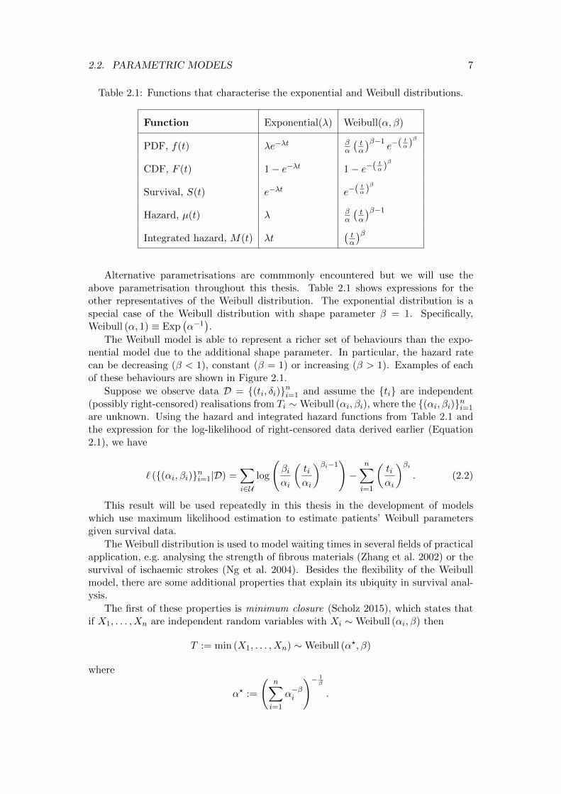
Table 2.1: Functions that characterise the exponential and Weibull distributions.
Function Exponential(λ) Weibull(α, β)
PDF, f(t) λe−λt βα
(tα
)β−1e−( tα)
β
CDF, F (t) 1− e−λt 1− e−( tα)β
Survival, S(t) e−λt e−( tα)β
Hazard, µ(t) λ βα
(tα
)β−1Integrated hazard, M(t) λt
(tα
)βAlternative parametrisations are commmonly encountered but we will use the
above parametrisation throughout this thesis. Table 2.1 shows expressions for theother representatives of the Weibull distribution. The exponential distribution is aspecial case of the Weibull distribution with shape parameter β = 1. Specifically,Weibull (α, 1) ≡ Exp
(α−1
).
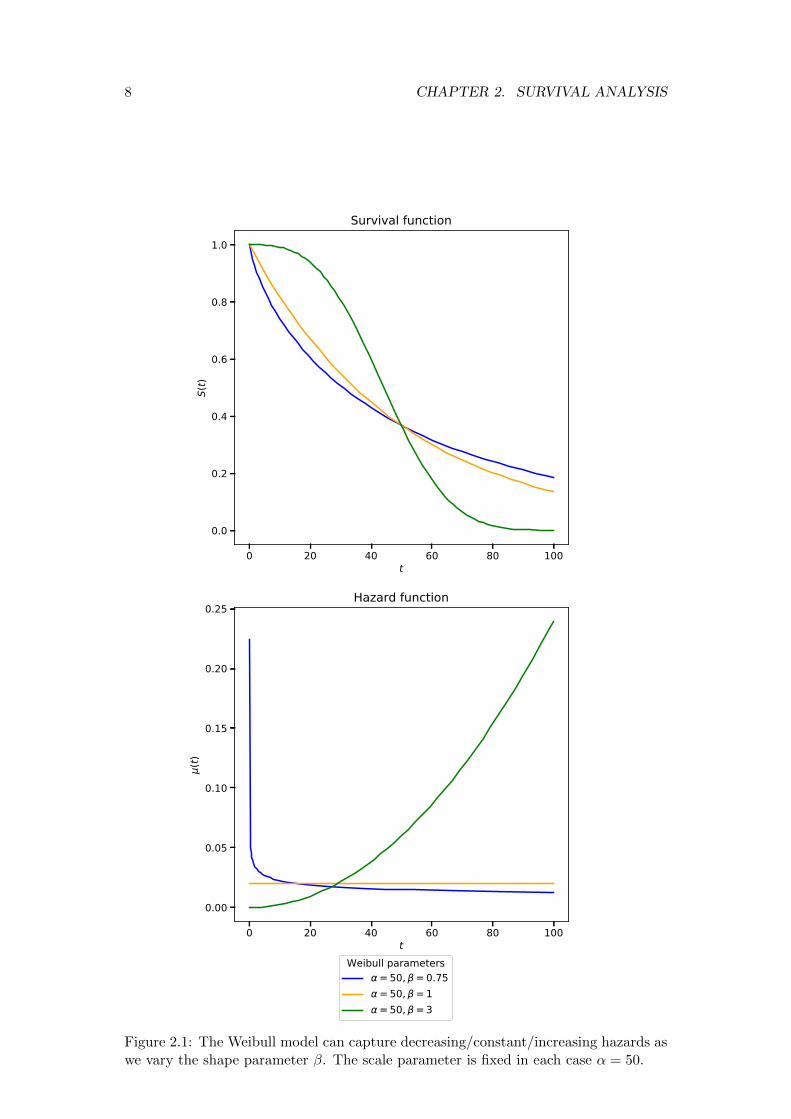
The Weibull model is able to represent a richer set of behaviours than the expo-nential model due to the additional shape parameter. In particular, the hazard ratecan be decreasing (β < 1), constant (β = 1) or increasing (β > 1). Examples of eachof these behaviours are shown in Figure 2.1.
Suppose we observe data D = {(ti, δi)}ni=1 and assume the {ti} are independent(possibly right-censored) realisations from Ti ∼Weibull (αi, βi), where the {(αi, βi)}ni=1
are unknown. Using the hazard and integrated hazard functions from Table 2.1 andthe expression for the log-likelihood of right-censored data derived earlier (Equation2.1), we have
` ({(αi, βi)}ni=1|D) =∑i∈U
log
(βiαi
(tiαi
)βi−1)−
n∑i=1
(tiαi
)βi. (2.2)
This result will be used repeatedly in this thesis in the development of modelswhich use maximum likelihood estimation to estimate patients’ Weibull parametersgiven survival data.
The Weibull distribution is used to model waiting times in several fields of practicalapplication, e.g. analysing the strength of fibrous materials (Zhang et al. 2002) or thesurvival of ischaemic strokes (Ng et al. 2004). Besides the flexibility of the Weibullmodel, there are some additional properties that explain its ubiquity in survival anal-ysis.
The first of these properties is minimum closure (Scholz 2015), which states thatif X1, . . . , Xn are independent random variables with Xi ∼Weibull (αi, β) then
T := min (X1, . . . , Xn) ∼Weibull (α?, β)
where
α? :=
(n∑i=1
α−βi
)− 1β
.
8 CHAPTER 2. SURVIVAL ANALYSIS
0 20 40 60 80 100t
0.0
0.2
0.4
0.6
0.8
1.0
S(t)
Survival function
0 20 40 60 80 100t
0.00
0.05
0.10
0.15
0.20
0.25
(t)
Hazard function
Weibull parameters= 50, = 0.75= 50, = 1= 50, = 3
Figure 2.1: The Weibull model can capture decreasing/constant/increasing hazards aswe vary the shape parameter β. The scale parameter is fixed in each case α = 50.
2.2. PARAMETRIC MODELS 9
This is easy to show via the survival function:
ST (t) = P (X1 > t, . . . ,Xn > t)
=n∏i=1
SXi(t)
=n∏i=1
exp
[−(t
αi
)β]
= exp
[−(t
α?
)β]which is precisely the survival function of a Weibull (α?, β) random variable.
This has a nice interpretation in the context of modelling survival times. Considera system comprising components whose lifetimes are independent and Weibull (withthe same shape parameter). If the system fails as soon as one of its components fails,then the system’s lifetime is Weibull.
In fact, we can relax the assumption that the individual components are Weibulland obtain a stronger result. To do this, we require the following definitions and resultsfrom Haan and Ferreira (2006) related to extreme value theory.
Definition 2.2.2 (Generalised extreme value distribution). The generalised extremevalue (GEV) distribution is the family of distributions with CDF
F (x;µ, σ, ξ) = exp
{−[1 + ξ
(x− µσ
)]− 1ξ
+
}where µ ∈ R, σ > 0, ξ ∈ R are the location, scale and shape parameters respectively,and y+ := max(y, 0)
The GEV family comprises three sub-families of distribution: Frechet (ξ > 0),Gumbel (ξ = 0) and reversed Weibull (ξ < 0).
Theorem 2.2.3 (Fisher-Tippett-Gnedenko). Let {Xi}∞i=1 be a sequence of independentidentically distributed random variables and Un := max(X1, . . . , Xn). Suppose thereexists a sequence of constants {(an, bn) : an > 0, bn ∈ R} such that
Un − bnan
D→ G
where G has a non-degenerate distribution. Then G is a member of the GEV family.
The following property, which Scholz (2015) refers to as the weakest link property,is a modification of Theorem 2.2.3. We now consider non-negative random variablesand the first failure time.
Corollary 2.2.4 (Weakest link property). Let Let X1, . . . , Xn be non-negative in-dependent and identically distributed random variables and Ln := min(X1, . . . , Xn).Suppose there exists a sequence of positive constants {an} such that
Lnan
D→ G
for some non-degenerate distribution G. Then G ∼Weibull.
10 CHAPTER 2. SURVIVAL ANALYSIS
Proof. Since X1, . . . , Xn ≥ 0 almost surely and the {an} are positive constants, Lnan ≥ 0
almost surely. Therefore if Ln/anD→ G and the distribution of G is non-generate, then
using Theorem 2.2.3 and the identity
max(X1, . . . , Xn) = −min(−X1, . . . ,−Xn),
H := −G is a member of the GEV family that is bounded above. The Gumbeland Frechet distribution have supports R and [0,∞) respectively. Therefore H ∼ReverseWeibull, and so G ∼Weibull.
This tells us that the lifetime of a system which fails as soon as one of its componentsfails may well be Weibull, even if the components’ lifetimes are not themselves Weibull.This suggests the Weibull distribution will be appropriate in many scenarios. Themodels developed in this thesis will be based on the Weibull distribution; the weakestlink property provides some rigorous basis for this choice of parametric distribution.
2.3 Performance metrics
In Section 3.1 we saw how traditional statistical methods need to be adapted to accountfor censoring. The same is true for metrics to evaluate models’ predictive performance.Performance metrics aim to quantify the discrepancy between predicted and actualoutcomes but censoring prevents us from fully observing the actual outcomes and thusnew measures designed for survival models are required. Section 2.3.1 will discussthe two types of predictive performance we can measure, namely discrimination andcalibration. Section 2.3.2 introduces the most popular metric, the concordance index,and its time-dependent extension. We will show how the concordance index arisesfrom recasting survival analysis as a ranking problem, and that the time-dependentconcordance index is a weighted-average of time-specific AUCs. Finally, the integratedBrier score is defined in Section 2.3.3.
2.3.1 Discrimination and calibration
Performance metrics generally incorporate one or both of two notions of predictiveperformance: discriminative and calibrative. (Steyerberg 2019, p. 251).
Discriminative performance relates to the model’s ability to discern between indi-viduals who experience the outcome and those who don’t. In the context of predictingsurvival times/distributions, discrimination relates to the task of distinguishing be-tween low- and high-risk individuals. Discrimination is not concerned with the exactpredicted/actual event times per se, but rather with how well the predicted orderingof death times (insofar as this exists) agrees with the realised ordering of death times(insofar as this is observed).
Calibrative performance relates to the degree of agreement between the predictedand observed outcomes. In other words, good calibration means the predicted survivaltime/distribution agree well with the actual survival time/distribution.
A model may perform well in one aspect but poorly on the other. For example,consider the (unattainable) model which predicts survival times perfectly. Then sup-pose we apply some (order-preserving) transformation to the predicted times. Themodel will retain its perfect discrimination, since the order of predicted event times
2.3. PERFORMANCE METRICS 11
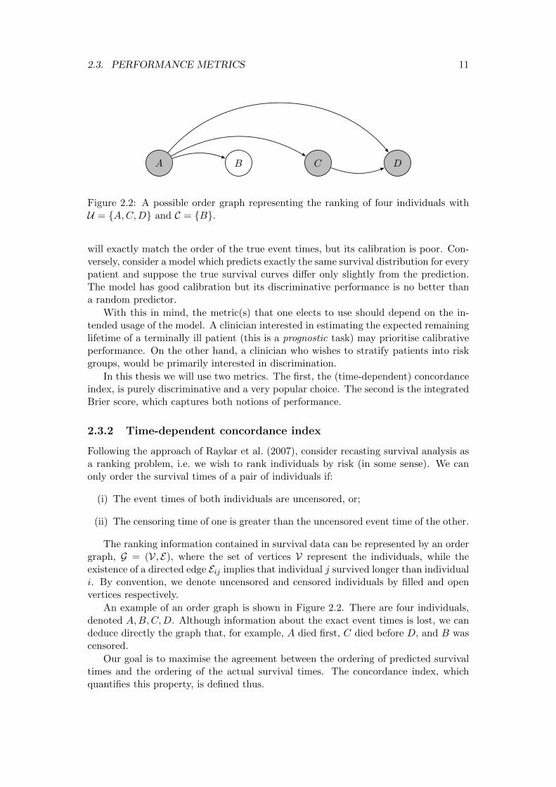
A B C D
Figure 2.2: A possible order graph representing the ranking of four individuals withU = {A,C,D} and C = {B}.
will exactly match the order of the true event times, but its calibration is poor. Con-versely, consider a model which predicts exactly the same survival distribution for everypatient and suppose the true survival curves differ only slightly from the prediction.The model has good calibration but its discriminative performance is no better thana random predictor.
With this in mind, the metric(s) that one elects to use should depend on the in-tended usage of the model. A clinician interested in estimating the expected remaininglifetime of a terminally ill patient (this is a prognostic task) may prioritise calibrativeperformance. On the other hand, a clinician who wishes to stratify patients into riskgroups, would be primarily interested in discrimination.
In this thesis we will use two metrics. The first, the (time-dependent) concordanceindex, is purely discriminative and a very popular choice. The second is the integratedBrier score, which captures both notions of performance.
2.3.2 Time-dependent concordance index
Following the approach of Raykar et al. (2007), consider recasting survival analysis asa ranking problem, i.e. we wish to rank individuals by risk (in some sense). We canonly order the survival times of a pair of individuals if:
(i) The event times of both individuals are uncensored, or;
(ii) The censoring time of one is greater than the uncensored event time of the other.
The ranking information contained in survival data can be represented by an ordergraph, G = (V, E), where the set of vertices V represent the individuals, while theexistence of a directed edge Eij implies that individual j survived longer than individuali. By convention, we denote uncensored and censored individuals by filled and openvertices respectively.
An example of an order graph is shown in Figure 2.2. There are four individuals,denoted A,B,C,D. Although information about the exact event times is lost, we candeduce directly the graph that, for example, A died first, C died before D, and B wascensored.
Our goal is to maximise the agreement between the ordering of predicted survivaltimes and the ordering of the actual survival times. The concordance index, whichquantifies this property, is defined thus.
12 CHAPTER 2. SURVIVAL ANALYSIS
Definition 2.3.1 (Concordance index). Given an order graph G = (V, E) and a set ofpredicted event times t1, . . . , tn, the concordance index (or c-index) is
c(G, t1, . . . , tn
)=
1
|E|∑Eij
1{ti < tj
}.
The concordance index is invariant under any order-preserving transformation ofthe predicted times, so clearly it is a purely discriminative metric. A model thatachieves c = 1 has perfect discriminative performance, while a random predictor wouldattain c = 0.5 (on average). As is usually the case in statistics, achieving perfectpredictive performance is nigh on impossible in practice. Even the (fictional) modelwhich learns the true survival distributions perfectly will (in general) fail to attainperfect ranking, attaining some c-index which is less than one, which we call the oraclec-index. In practice it is only possible to compute the oracle c-index when the truesurvival curves are known, i.e. when we are working with simulated data. We will seethis in practice in Chapter 6.
t
µ(t)
(a) In a PH model, the ordering of hazardfunctions never changes.
t
µ(t)
(b) For more general/flexible models thehazard functions may overlap, so there isno natural way to order the risks.
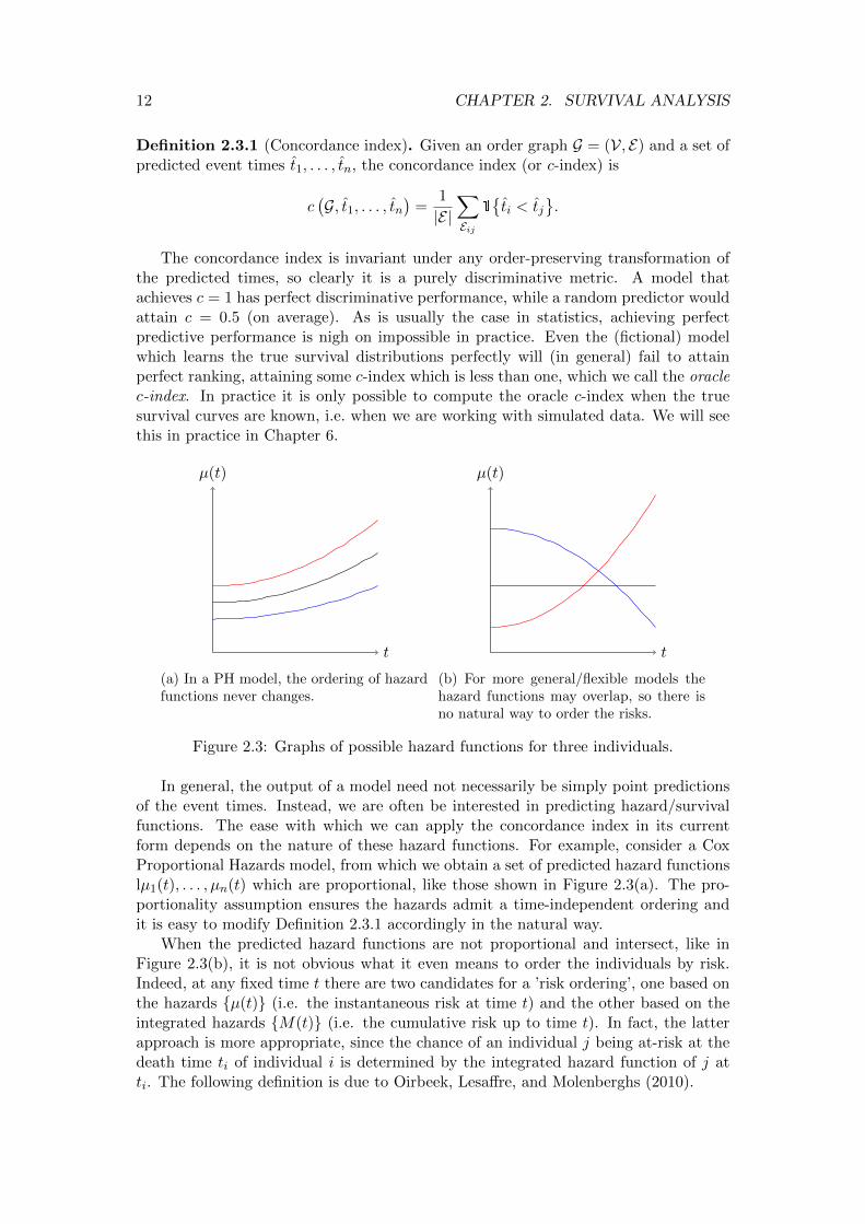
Figure 2.3: Graphs of possible hazard functions for three individuals.
In general, the output of a model need not necessarily be simply point predictionsof the event times. Instead, we are often be interested in predicting hazard/survivalfunctions. The ease with which we can apply the concordance index in its currentform depends on the nature of these hazard functions. For example, consider a CoxProportional Hazards model, from which we obtain a set of predicted hazard functionslµ1(t), . . . , µn(t) which are proportional, like those shown in Figure 2.3(a). The pro-portionality assumption ensures the hazards admit a time-independent ordering andit is easy to modify Definition 2.3.1 accordingly in the natural way.
When the predicted hazard functions are not proportional and intersect, like inFigure 2.3(b), it is not obvious what it even means to order the individuals by risk.Indeed, at any fixed time t there are two candidates for a ’risk ordering’, one based onthe hazards {µ(t)} (i.e. the instantaneous risk at time t) and the other based on theintegrated hazards {M(t)} (i.e. the cumulative risk up to time t). In fact, the latterapproach is more appropriate, since the chance of an individual j being at-risk at thedeath time ti of individual i is determined by the integrated hazard function of j atti. The following definition is due to Oirbeek, Lesaffre, and Molenberghs (2010).
2.3. PERFORMANCE METRICS 13
Definition 2.3.2 (Time-dependent concordance index). Given an order graph G =(V, E), event/censoring times t1, . . . , tn and predicted survival functions S1, . . . Sn, thetime-dependent concordance index is
ctd(G, S1, . . . Sn
)=
1
|E|∑Eij
1
{Si(ti) < Sj(ti)
}.
If hazards are proportional, the concordance index and time-dependent concor-dance index coincide. Although the definition is framed in terms of predicted survivalfunctions {Si}, it is straightforward to adapt it for, say, predicted integrated hazardfunctions by applying the relation S(t) = exp(−M(t)) and reversing the inequalityin the indicator function, since x 7→ e−x is strictly decreasing and therefore order-reversing.
The time-dependent concordance index is a single number which encapsulates amodel’s discriminative capabilities. Generally, a model’s ability to discriminate be-tween subjects can vary over time. Gaining insight into this behaviour may be usefuland enable a more nuanced comparison between models. In fact, Antolini, Boracchi,and Biganzoli (2005) have shown that the time-dependent concordance index can beequivalently expressed as a weighted average of time-specific AUCs (i.e. the area undera ROC curve).
Consider a set of a set of predicted survival functions S1, . . . , Sn and a set ofdiscrete time points T . Fix t ∈ T . For some v ∈ [0, 1], we can consider Si as defininga prediction rule:
Si(t) ≤ v =⇒ predict ”individual i dead at t”;
Si(t) > v =⇒ predict ”individual i alive at t”.
This defines a binary classification test. The notion of sensitivity (the true positiverate) refers to the the probability of correctly predicting that an individual is deadat time t, and specificity (the true negative rate) relates to correctly predicting anindividual is alive at time t. The (time-specific) AUC is given by
AUC(t) =
∑i 6=j 1{Si(t) < Sj(t)}1{ti ≤ t, δi = 1, tj > t}∑
i 6=j 1{ti ≤ t, δi = 1, tj > t}.
We weight the time-specific AUC according to the proportion of comparable pairsavailable at that time, which is given by
w(t) =
∑i 6=j 1{ti ≤ t, δi = 1, tj > t}∑
s∈T∑
i 6=j 1{ti ≤ s, δi = 1, tj > s}.
The weights are defined such that∑
t∈T w(t) = 1. The time-concordance index isequivalent to the weighted average of the time-specific AUCs,
ctd =∑t∈T
w(t) ·AUC(t).
2.3.3 Integrated Brier score
The second performance metric that we consider is the integrated Brier score, whichwill complement the c-index by accounting for calibrative performance. We start by
14 CHAPTER 2. SURVIVAL ANALYSIS
defining the Brier score from traditional statistics, then show how this can be modifiedfor survival data, and finally define the integrated Brier score.
The Brier score is used in traditional statistics to measure the accuracy of prob-abilistic predictions on a set of outcomes. The metric, which was developed in thecontext of assessing probabilistic weather predictions, was originally formulated byBrier (1950).
Definition 2.3.3 (Brier score). Suppose that on n occassions an event occurs inexactly one of r classes, which are mutually exclusive and exhaustive. Given predictedprobabilities {Pij} for each occasion i = 1, . . . , n and class j = 1, . . . , r, the Brier scoreis given by
BS =1
n
n∑i=1
r∑j=1
(Pij − Eij
)2where Eij = 1 if the event on occasion i occurred in class j, and zero otherwise.
The Brier score measures the mean squared error between the predicted probabil-ities and the actual outcomes. A lower Brier score indicates better performance.
Kvamme, Borgan, and Scheel (2019) explain how to modify the Brier score forapplication to survival data. The idea is to use the Brier score to measure how well themodel predicts whether individuals survive beyond a fixed time t. We can categoriseindividuals (except those who are censored before time t) into two classes according towhether they died before t or survived past t. This is the intuition behind the Brierscore for survival data.
Definition 2.3.4 (Brier score for survival data). Fix a time t. Given data {(ti, δi,xi)}ni=1
and predicted survival functions S1, . . . , Sn, the Brier score with respect to t is
BS (t) =1
n
n∑i=1
[Si(t)
2 · 1{ti ≤ t, δi = 1}G(ti)
+[1− Si(t)]2 · 1{ti > t}
G(t)
]
where G(·) is the Kaplan-Meier estimate of the survival function of the censoringdistribution.
In fact, this is more properly referred to as the inverse probability-of-censoringweighed (IPCW) Brier score, due to the factors 1/G(·). Kvamme and Borgan (2019)explains that the weights ensure the IPCW Brier score retains some of the propertiesof the Brier score for uncensored data.
The Brier score in its current form isn’t particularly useful because it only gives asnapshot of predictive performance with reference to the arbitrary time point t. Theintegrated Brier score remedies this problem by averaging the Brier score over a timeinterval.
Definition 2.3.5 (Integrated Brier score). Fix 0 ≤ T1 < T2. Then the integratedBrier score is
IBS =1
T2 − T1
∫ T2
T1
BS(t) dt.
In practice, we typically set T1 = 0 and T2 = max{ti} and approximate the integralusing numerical methods. Alternatively, we may decide to choose a smaller value forT2 to improve stability of the metric, since as t → T2 there will be fewer individualsat risk and the the Brier score BS(t) will become unstable, which could distort theoverall metric.
Chapter 3
Neural networks
In this chapter, we briefly review some basic concepts related to neural networks thatwill be used in this thesis. In particular, we discuss some of the common activationfunctions (Section 3.1.1), recap the idea of loss functions (Section 3.1.2) and explainneural network validation methods (Section 3.1.3). For a more complete introductionto neural networks consult Hastie, Tibshirani, and Friedman (2009), upon which thematerial in this chapter is primarily based.
3.1 Basic concepts
Neural networks belong to a class of non-linear statistical models, where the idea is toform derived features from linear combinations of the inputs, and model the target as anon-linear function of these features. Neural networks can be used for both regressionand classification.
3.1.1 Activation functions
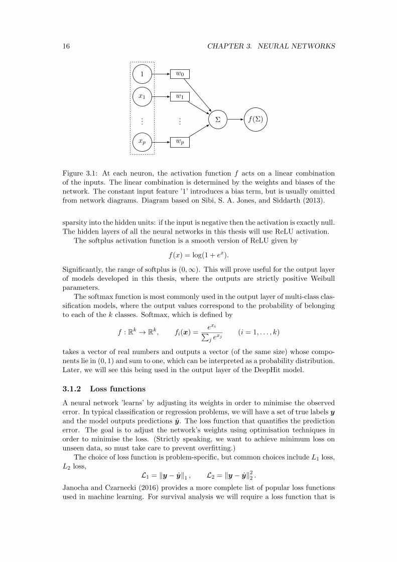
Activation functions are used to transform the activation level of a neuron to an outputsignal. This is represented schematically in Figure 3.1, where the {xi} are the features,{wi} are the weights of the model (to be determined) and f(·) is a suitably chosenactivation function.
Activation functions allow us to directly introduce non-linearity into the model andcontrol the range of the outputs. Sibi, S. A. Jones, and Siddarth (2013) review the vastarray of activation functions that are commonly used and how they perform. Theyconclude that choosing activation functions is of secondary importance compared toconsiderations such as tuning the network size (the number of layers and their widths)and the learning hyperparameters. In this thesis we will only make use of three commonactivation functions: ReLU, softplus and softmax. We now briefly discuss each of thesefunctions in turn, and their key properties/advantages, as given in Nwankpa et al.(2018).
The rectified linear unit (ReLU) is a piecewise linear function given by
f(x) = max(0, x).
It is the most commonly used activation function in machine learning and achievesgood performance in general. A key reason for choosing ReLU is computational speed- there is no need to perform exponentiation or division. Moreover, ReLU introduces
15
16 CHAPTER 3. NEURAL NETWORKS
1
x1
...
xp
w0
w1
...
wp
Σ f(Σ)
Figure 3.1: At each neuron, the activation function f acts on a linear combinationof the inputs. The linear combination is determined by the weights and biases of thenetwork. The constant input feature ’1’ introduces a bias term, but is usually omittedfrom network diagrams. Diagram based on Sibi, S. A. Jones, and Siddarth (2013).
sparsity into the hidden units: if the input is negative then the activation is exactly null.The hidden layers of all the neural networks in this thesis will use ReLU activation.
The softplus activation function is a smooth version of ReLU given by
f(x) = log(1 + ex).
Significantly, the range of softplus is (0,∞). This will prove useful for the output layerof models developed in this thesis, where the outputs are strictly positive Weibullparameters.
The softmax function is most commonly used in the output layer of multi-class clas-sification models, where the output values correspond to the probability of belongingto each of the k classes. Softmax, which is defined by
f : Rk → Rk, fi(x) =exi∑j e
xj(i = 1, . . . , k)
takes a vector of real numbers and outputs a vector (of the same size) whose compo-nents lie in (0, 1) and sum to one, which can be interpreted as a probability distribution.Later, we will see this being used in the output layer of the DeepHit model.
3.1.2 Loss functions
A neural network ’learns’ by adjusting its weights in order to minimise the observederror. In typical classification or regression problems, we will have a set of true labels yand the model outputs predictions y. The loss function that quantifies the predictionerror. The goal is to adjust the network’s weights using optimisation techniques inorder to minimise the loss. (Strictly speaking, we want to achieve minimum loss onunseen data, so must take care to prevent overfitting.)
The choice of loss function is problem-specific, but common choices include L1 loss,L2 loss,
L1 = ‖y − y‖1 , L2 = ‖y − y‖22 .Janocha and Czarnecki (2016) provides a more complete list of popular loss functionsused in machine learning. For survival analysis we will require a loss function that is
3.1. BASIC CONCEPTS 17
able to incorporate censored data, such as the (negative) log-likelihood for censoreddata that we derived in Chapter 2.
3.1.3 Training and testing
Ultimately, our goal is to develop a model which achieves good predictive performanceon unseen data. This can be broken down into two steps. The first, model selection,involves assessing the performance of various models in order to find the optimal model.In the second step, model assessment, we estimate the performance of the optimalmodel on unseen data.
The ’holdout’ approach involves randomly dividing the data into three parts: train-ing data, validation data, and test data. We fit the models using the training data,perform model selection based on the prediction error on the validation set, and assessthe optimal model using the test set. It is crucial that the test data is only used formodel assessment, and that no ’contamination’ occurs, whereby test data is used inthe training of the model. The appropriate relative proportions of the train/valida-tion/test split will generally be based on the size of the data set and its signal-to-noiseratio.
The holdout method is simple and computationally cheap. However, the results weobtain will depend on the train/test split. If we only perform the process once, theremay be large error in our estimate of the prediction error. To counter this we maytake the average over multiple runs of the holdout method, or use more sophisticatedapproaches of cross-validation, e.g. k-folds cross validation.
Chapter 4
Survey: neural networks insurvival analysis
This chapter reviews some existing approaches to applying neural networks to survivalanalysis that have been proposed in the literature. For a more in-depth survey (in-cluding machine learning methods more widely) see Wang, Li, and Reddy (2019). InSection 4.1 we formulate the Cox proportional hazards model and then outline theneural network extensions developed by Faraggi and Simon (1995) and Katzman et al.(2016). Section 4.2 looks at so-called classification methods, such as those proposedby Liestøl, Kragh, and Andersen (1994) and Biganzoli et al. (1998). The chapter con-cludes (Section 4.3) with an in-depth review of DeepHit, a novel approach by Lee et al.(2018a). By evaluating the pros and cons of each approach, we identify a potential’niche’ which our proposed model seeks to fill.
4.1 Cox model approaches
In this section we review two neural net methods developed by Faraggi and Simon(1995) and Katzman et al. (2016). Both algorithms are based on the Cox proportionalhazards model, which we introduce now.
4.1.1 Cox proportional hazards model
The Cox proportional hazards model is a semi-parametric survival model due to Cox(1972). Given an individual with covariates x = (x1, . . . , xp)
T , the hazard function ismodelled by
λ(t;x) = λ0(t) exp(βTx) (4.1)
where β = (β1, . . . , βp)T is a regression vector and λ0(t) is an unspecified baseline
hazard function corresponding to individuals with x = 0. The baseline hazard isusually considered a nuisance parameter and the vector of parameters is estimated bymaximising the partial likelihood
L(β) =∏i∈U
exp(βTxi)∑j∈Ri exp(βTxj)
where Ri is the set of at-risk individuals at the event time of individual i.
18
4.1. COX MODEL APPROACHES 19
1
x1
x2
...
xp
z1
z2
...
zm
y
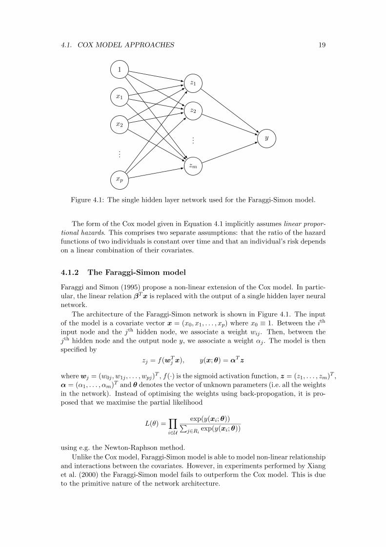
Figure 4.1: The single hidden layer network used for the Faraggi-Simon model.
The form of the Cox model given in Equation 4.1 implicitly assumes linear propor-tional hazards. This comprises two separate assumptions: that the ratio of the hazardfunctions of two individuals is constant over time and that an individual’s risk dependson a linear combination of their covariates.
4.1.2 The Faraggi-Simon model
Faraggi and Simon (1995) propose a non-linear extension of the Cox model. In partic-ular, the linear relation βTx is replaced with the output of a single hidden layer neuralnetwork.
The architecture of the Faraggi-Simon network is shown in Figure 4.1. The inputof the model is a covariate vector x = (x0, x1, . . . , xp) where x0 ≡ 1. Between the ith
input node and the jth hidden node, we associate a weight wij . Then, between thejth hidden node and the output node y, we associate a weight αj . The model is thenspecified by
zj = f(wTj x), y(x;θ) = αTz
wherewj = (w0j , w1j , . . . , wpj)T , f(·) is the sigmoid activation function, z = (z1, . . . , zm)T ,
α = (α1, . . . , αm)T and θ denotes the vector of unknown parameters (i.e. all the weightsin the network). Instead of optimising the weights using back-propogation, it is pro-posed that we maximise the partial likelihood
L(θ) =∏i∈U
exp(y(xi;θ))∑j∈Ri exp(y(xi;θ))
using e.g. the Newton-Raphson method.
Unlike the Cox model, Faraggi-Simon model is able to model non-linear relationshipand interactions between the covariates. However, in experiments performed by Xianget al. (2000) the Faraggi-Simon model fails to outperform the Cox model. This is dueto the primitive nature of the network architecture.
20 CHAPTER 4. SURVEY: NEURAL NETWORKS IN SURVIVAL ANALYSIS
4.1.3 DeepSurv
A modernised version of the Faraggi-Simon network, called DeepSurv, was developedby Katzman et al. (2016). DeepSurv uses multiple hidden layers and leverages modernneural network techniques including ReLU activation and batch normalisation. Thenegative log partial likelihood is used as a loss function.
As expected, when the risk function is non-linear in the covariates DeepSurv demon-strates superior predictive performance to the Cox model.
4.1.4 Discussion
The Cox model approaches demonstrate how neural networks can be employed insurvival analysis to adapt traditional statistical techniques and improve predictions.By leveraging neural networks’ ability to learn non-linear relationships, the models areable to represent more complicated covariate-risk relationships.
The neural network extensions of the Cox model have some drawbacks. First, aswith any flexible modelling approach, there is much greater potential for overfitting.Second, the parameters of a neural network model are harder to interpret than theregression parameter of the Cox model and there is less scope to test the statisticalsignificance of the explanatory variable in relation to survival. Third, this approachretains the assumption of proportional hazards, which is restrictive and often invalidwhen the number of covariates is large (Zhao and Feng 2020).
4.2 Classification approaches
Classification methods form an entirely different branch of neural network approachesto survival analysis, which are based on discrete-time (or grouped) survival data. Thissection reviews two such approaches by Liestøl, Kragh, and Andersen (1994) andBiganzoli et al. (1998).
4.2.1 Framework
Classification methods are based on survival data where the event time is grouped intodisjoint intervals. In particular, we form a partition 0 = t0 < t1 < . . . < tm < ∞ anddefine Ik = [tk−1, tk] for k = 1, . . . ,m. Then the log-likelihood function based on nindividuals is given by
` = −n∑i=1
mi∑k=1
[Dki log pk(xi) + (1−Dki) log(1− pk(xi))] (4.2)
where mi ≤ m is the number of intervals in which patient i is observed, Dki is anindicator for individual i dying in interval Ik, and
pk(x) = P (T < tk|T ≥ tk−1) , (k = 1, . . . ,m)
is the conditional death probability for an individual with covariate vector x.
Both of the models we consider use neural networks to predict the conditional deathprobabilities, i.e. the the discrete hazard function.
4.2. CLASSIFICATION APPROACHES 21
4.2.2 Liesøl model
Liestøl, Kragh, and Andersen (1994) propose using a neural network with p inputnodes (the covariates) and m output nodes (one for each predicted conditional deathprobability). An activation function which takes values in [0, 1], e.g. logistic activation,is applied to the output layer. The network is trained using Di = (D1i, . . . , Dmii) asthe target and a loss function based on the log-likelihood function (4.2).
Unlike the Cox-based models, the Liesøl approach allows for a range of assump-tions about the hazard rate. The linear proportional hazards assumption can be im-plemented by using no hidden layers and imposing certain restrictions on the weights.Adding hidden layers introduces non-linearity, while relaxing the restrictions on theweights allows for non-proportionality.
In the linear proportional hazards setting, by choosing the appropriate activationfunction the Liesøl model becomes equivalent to the discrete-time survival models pro-posed by Cox (1972) or Prentice and Gloeckler (1978). Hence, like the Cox model ap-proaches, the Liesøl model can be viewed as a generalisation of traditional approaches.
4.2.3 Partial logistic regression models with ANN (PLANN)
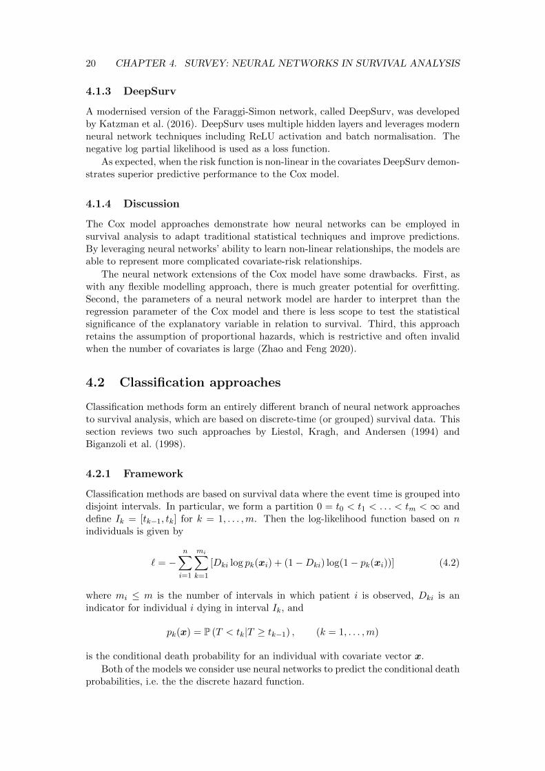
The Liesøl model was further developed by Biganzoli et al. (1998). They proposea radically different network architecture, which is shown in Figure 4.2. The maindifference is that the conditional death probabilities are now estimated individuallyand the index of the time interval is used as an explanatory variable.
These modifications yield several benefits. By using time as an input variable,PLANN is able to obtain smoothed estimates of the hazard rate and handle time-dependent covariates. The PLANN network is simpler to implement since the numberof target elements is now constant (one) rather than depending on the number ofintervals for which an individual was at-risk.
1
x1
...
xp
k
1
z1
...
zm
pk
Figure 4.2: The PLANN network with one hidden layer for estimating the conditionaldeath probability in interval Ik. In general, the covariates could be time-dependentxi = xi(k).
22 CHAPTER 4. SURVEY: NEURAL NETWORKS IN SURVIVAL ANALYSIS
4.2.4 Discussion
Similar to the Cox-based models, classification methods use neural networks to ex-tend traditional survival models and model non-linear relationships between the co-variates and the hazard function. However, classification approaches can also modelnon-proportional hazards, which adds greater flexibility. Experiments by Biganzoliet al. (1998) confirm this flexibility pays off on real-world data with complex covariateinteractions. The usual drawbacks (chance of overfitting, lack of interpretability, etc.)of flexible modelling approaches apply.
A major downside of these approaches is that they do not handle continuous-time survival data. Grouping survival data will necessarily entail information loss, andchoosing the granularity of the partition will involve a trade-off between the smoothnessof the resulting hazard function estimate and considerations of computational cost.The hazard function output by the model may require (further) smoothing and haveinterpretability issues.
Both models predict the survival distribution by estimating the conditional eventprobabilities or discrete hazard function. Alternatives such as the discrete survivalfunction are available and it is not obvious whether one option is better than theother.
4.3 DeepHit
DeepHit is a state-of-the-art deep learning approach to survival analysis, upon whichthe model proposed in this thesis is largely inspired. This section entails an in-depthreview of the model, including setting up notation (Section 4.3.1), studying the config-uration of the neural network (Section 4.3.2), explaining the loss function 4.3.3) andthe training process (Section 4.3.4), and examining the performance gains achievedover competitors (Section 4.3.5). The final discussion (Section 4.3.6) will aim to iden-tify the strengths and weaknesses of the model. The material in this section is basedon Lee et al. 2018a and Lee et al. 2018b.
4.3.1 Framework and notation
Suppose we are in a competing risks setting with K ≥ 1 possible events, exactlyone of which will eventually occur. We write the set of possible outcomes as K ={0, 1, . . . ,K}, where the outcome 0 denotes a right-censored observation.
The survival time is treated as discrete and bounded by some predetermined timehorizon Tmax. The index set of possible event times is T = {0, 1, . . . , Tmax}. Althoughan equidistant partition of [0, Tmax] is a reasonable way to discretise continuous-timedata, a partition based on empirical quantiles may be more appropriate because sur-vival data tends to be positively skewed.
We are given survival data D = {(ti, ki,xi)}ni=1 where ti ∈ T is the time of theoutcome ki ∈ K and xi denotes a p-vector of covariates. Given an unseen individualwith covariates x?, the goal is to estimate the probabilities
P (t = t?, k = k?|x = x?)
for all times t? ∈ T and all events k? ∈ K \ {0}.
4.3. DEEPHIT 23
x
fs
z
fc1
...
fcK
y L D
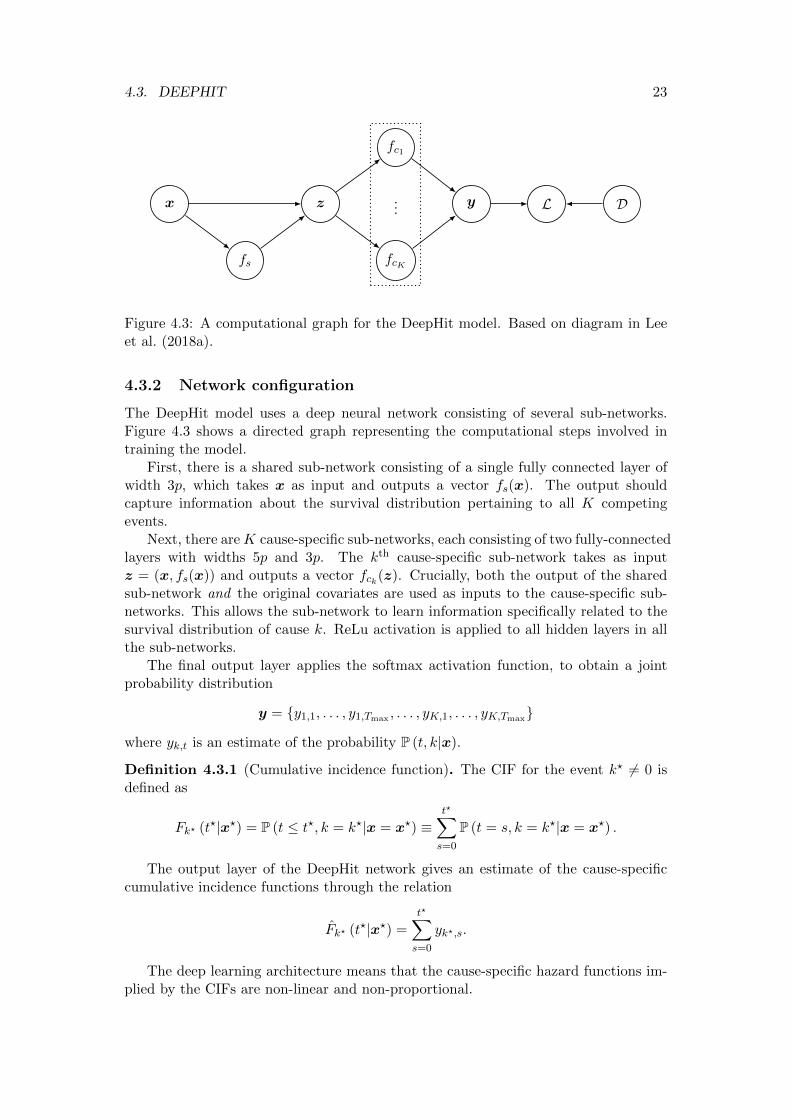
Figure 4.3: A computational graph for the DeepHit model. Based on diagram in Leeet al. (2018a).
4.3.2 Network configuration
The DeepHit model uses a deep neural network consisting of several sub-networks.Figure 4.3 shows a directed graph representing the computational steps involved intraining the model.
First, there is a shared sub-network consisting of a single fully connected layer ofwidth 3p, which takes x as input and outputs a vector fs(x). The output shouldcapture information about the survival distribution pertaining to all K competingevents.
Next, there areK cause-specific sub-networks, each consisting of two fully-connectedlayers with widths 5p and 3p. The kth cause-specific sub-network takes as inputz = (x, fs(x)) and outputs a vector fck(z). Crucially, both the output of the sharedsub-network and the original covariates are used as inputs to the cause-specific sub-networks. This allows the sub-network to learn information specifically related to thesurvival distribution of cause k. ReLu activation is applied to all hidden layers in allthe sub-networks.
The final output layer applies the softmax activation function, to obtain a jointprobability distribution
y = {y1,1, . . . , y1,Tmax , . . . , yK,1, . . . , yK,Tmax}
where yk,t is an estimate of the probability P (t, k|x).
Definition 4.3.1 (Cumulative incidence function). The CIF for the event k? 6= 0 isdefined as
Fk? (t?|x?) = P (t ≤ t?, k = k?|x = x?) ≡t?∑s=0
P (t = s, k = k?|x = x?) .
The output layer of the DeepHit network gives an estimate of the cause-specificcumulative incidence functions through the relation
Fk? (t?|x?) =t?∑s=0
yk?,s.
The deep learning architecture means that the cause-specific hazard functions im-plied by the CIFs are non-linear and non-proportional.
24 CHAPTER 4. SURVEY: NEURAL NETWORKS IN SURVIVAL ANALYSIS
The focus of this thesis will be single-event survival data. In the case k = 1, theDeepHit network configuration comprises one input layer, three hidden layers and asoftmax output layer. The widths of the hidden layers are 3p, 5p and 3p respectively,all using ReLU activation function.
4.3.3 Loss function
DeepHit is trained using a loss function of the form
L = L1 + αL2
where α ≥ 0 is a hyperparameter to be chosen, L1 is based on the log-likelihoodfunction and L2 is a ranking loss function.
The first component L1 of the total loss is the negative log-likelihood for right-censored data for the joint distribution of the first hitting time and event. For eachindividual i ∈ U , denote by y(i) the element of the softmax layer corresponding to theobserved event and event time for individual i, i.e.
y(i) = yki,ti(xi) = P (ti, ki|xi) .
Then the loss function L1 is given by
L1 = −n∑i=1
[1{ki = 0} · log
(1−
K∑k=1
Fk (ti|xi)
)+ 1{ki 6= 0} · log
(y(i))]
.
The L1 penalty drives the model to learn the true survival distribution.The second term L2 in the total loss function incorporates the idea of concordance
to measure ranking loss. In particular, define
Ak,i,j := 1{ki = k, ti < tj}
η(x, y) := exp
(−x− y
σ
)where k 6= 0 and σ > 0 is a hyperparameter. Here Ak,i,j indicates whether individualsi and j are comparable for event k and η(·, ·) is a convex loss function. Then the losscomponent is given by
L2 =K∑k=1
∑i 6=j
Ak,i,j · η(Fk (ti|xi) , Fk (ti|xj)
).
The Ak,i,j term checks whether individuals i and j are comparable with respect toevent k, and then η(·, ·) penalises incorrect orderings of such pairs. This improves themodel’s discriminative performance.
The hyperparameter α controls the relative importance of the the two loss func-tions. Its influence on model performance will be discussed in Sections 4.3.5 and 4.3.6.
4.3.4 Training the neural network
The network is trained using back-propogation via the Adam optimiser, using a batchsize of 50 and a learning rate of 10−4. Xavier initialisation and dropout probability of0.6 is applied to each layer. The original authors implemented DeepHit in a Tensorflowenvironment. In this thesis, we use the PyTorch implementation in the Python packagepycox.
4.3. DEEPHIT 25
4.3.5 Results
The original authors tested the model on one simulated dataset and three real-worlddatasets. Predictive performance is measured by a competing risks extension the time-dependent concordance index, where the c-index for cause k is given by
ctdk =
∑i 6=j Ak,i,j · 1
{Fk (ti|xi) > Fk (ti|xj)
}∑
i 6=j Ak,i,j, (k = 1, . . . ,K).
In the absence of other performance metrics, we have no indication of DeepHit’s cal-ibrative performance. The full results can be found in Lee et al. (2018a), which com-pares DeepHit with a range of existing methods from the literature. DeepHit generallyachieves superior performance for both single risk and competing risks datasets. This isattributed to the lack of assumptions regarding the the underlying stochastic process orthe relationship between the covariates and hazards compared with other approaches.
Lee et al. 2018b explores the performance effect of varying the hyperparameter α inthe loss function. Unsurprisingly, the model which utilises ranking loss (α 6= 0) achievesbetter discriminative performance than that which doesn’t (α = 0). Experiments shedlight on exactly where this gain occurs: since L2 penalises incorrect orderings, itsinclusion drives the model to focus on the time intervals with a high frequency ofobserved events where discrimination is most challenging.
4.3.6 Discussion
DeepHit establishes its advantage over competitors by imposing assumptions on nei-ther the underlying stochastic process nor the relationship between the covariates andthis process, and employing a modern deep learning architecture to learn this relation-ship. Moreover, its ability to handle competing risks distinguishes DeepHit from mostexisting methods.
Most of the datasets used to test DeepHit have a large number of patients. Ofthe four datasets experimented upon, three contained at least 30,000 individuals andthe smallest dataset had approximately 2,000 patients. This is not representative ofsurvival data encountered in the real-world: clinical trials often have small samplesizes due to, for example, the low prevalence of the disease of interest or trial designconsiderations (Xu 2017). As with any neural network method, we would expectDeepHit to perform best when training data is abundant, but it is important to testwhat happens when this is not the case.
Another point of discussion is the loss function. In particular, Raykar et al. 2007 arecritical of the approach of incorporating a ranking penalty term. In certain contexts,such as patient risk stratification in order to inform clinical decisions, achieving gooddiscriminative performance may be considered the primary goal. However, usually theoverarching objective is to learn survival distributions. It is true that well-calibratedmodels will tend to discriminate well - though not always - and therefore it is whollyappropriate to use the concordance index as a performance metric. Ultimately, how-ever, the purpose of the model is not to solve a ranking problem, and therefore theinclusion of L2 in the loss function seems questionable.
Similar to the classification methods discussed in Section 4.2, DeepHit is a discrete-time approach. Continuous-time data will require discretisation and the estimatedsurvival curves are not smooth, which may cause interpretability issues. However,

26 CHAPTER 4. SURVEY: NEURAL NETWORKS IN SURVIVAL ANALYSIS
unlike the Liesøl and PLANN models, DeepHit uses the cumulative incidence functionas the basis of the model output instead of the hazard function. This also contrastswith other competing risks survival models: the Fine-Gray model (Fine and Gray1999) and the regression models detailed by Haller, Schmidt, and Ulm (2013) are alsobased on the cause-specific/sub-distribution hazard. No justification is given for thischoice and the effect on performance, if any, is not clear.
Chapter 5
Proposed model
Having covered the requisite material and studied previous work in the field, we arenow ready to introduce the proposed model. This new approach, which we call Deep-Weibull, uses a deep neural network to fit a Weibull survival distribution. In Section5.1 we describe the setup and the network configuration. Section 5.2 formulates the lossfunction, states some of its properties such as a unique global optimum and instabilityunder highly-censored data, and looks at opportunities for regularisation. We conclude(Section 5.3) with a discussion of potential extensions to the model and describe whereit might be expected to perform well/poorly.
5.1 Model description
This section describes the model structure the configuration of the neural network.
5.1.1 Framework and notation
DeepWeibull is designed for single-event, continuous-time survival data. We are givensurvival data D = {ti, δi,xi}ni=1 where the xi are p-vectors of covariates. We assumethe data-generating process follows a Weibull distribution. The goal is to predict,given the covariates x of a (new) patient, the Weibull parameters α, β > 0 which fullycharacterise their survival distribution. The resulting survival curves are smooth anddefined on R+.
5.1.2 Network configuration
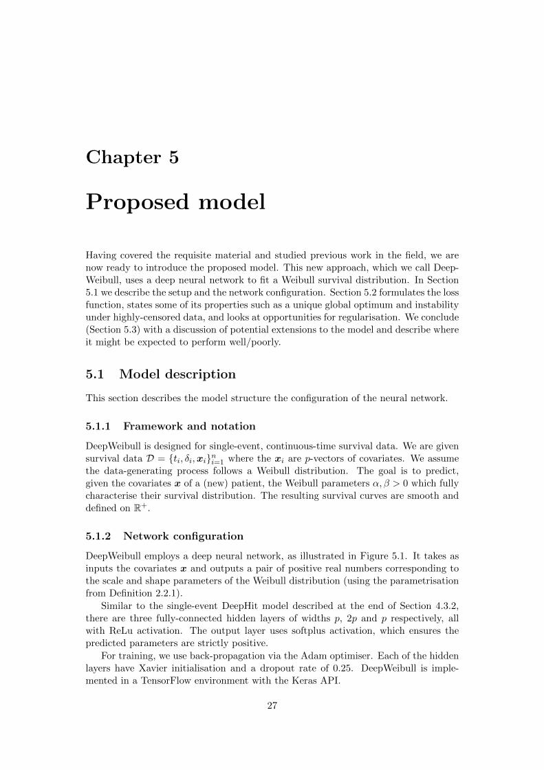
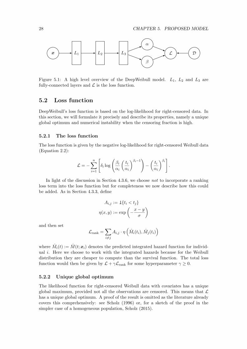
DeepWeibull employs a deep neural network, as illustrated in Figure 5.1. It takes asinputs the covariates x and outputs a pair of positive real numbers corresponding tothe scale and shape parameters of the Weibull distribution (using the parametrisationfrom Definition 2.2.1).
Similar to the single-event DeepHit model described at the end of Section 4.3.2,there are three fully-connected hidden layers of widths p, 2p and p respectively, allwith ReLu activation. The output layer uses softplus activation, which ensures thepredicted parameters are strictly positive.
For training, we use back-propagation via the Adam optimiser. Each of the hiddenlayers have Xavier initialisation and a dropout rate of 0.25. DeepWeibull is imple-mented in a TensorFlow environment with the Keras API.
27
28 CHAPTER 5. PROPOSED MODEL
x L1 L2 L3
α
β
L D
Figure 5.1: A high level overview of the DeepWeibull model. L1, L2 and L3 arefully-connected layers and L is the loss function.
5.2 Loss function
DeepWeibull’s loss function is based on the log-likelihood for right-censored data. Inthis section, we will formulate it precisely and describe its properties, namely a uniqueglobal optimum and numerical instability when the censoring fraction is high.
5.2.1 The loss function
The loss function is given by the negative log-likelihood for right-censored Weibull data(Equation 2.2):
L = −n∑i=1
[δi log
(βiαi
(tiαi
)βi−1)−(tiαi
)βi].
In light of the discussion in Section 4.3.6, we choose not to incorporate a rankingloss term into the loss function but for completeness we now describe how this couldbe added. As in Section 4.3.3, define
Ai,j := 1{ti < tj}
η(x, y) := exp
(−x− y
σ
)and then set
Lrank =∑i 6=j
Ai,j · η(Mi(ti), Mj(ti)
)where Mi(t) := M(t;xi) denotes the predicted integrated hazard function for individ-ual i. Here we choose to work with the integrated hazards because for the Weibulldistribution they are cheaper to compute than the survival function. The total lossfunction would then be given by L+ γLrank for some hyperparameter γ ≥ 0.
5.2.2 Unique global optimum
The likelihood function for right-censored Weibull data with covariates has a uniqueglobal maximum, provided not all the observations are censored. This means that Lhas a unique global optimum. A proof of the result is omitted as the literature alreadycovers this comprehensively: see Scholz (1996) or, for a sketch of the proof in thesimpler case of a homogeneous population, Scholz (2015).
5.3. DISCUSSION 29
5.2.3 Numerical instability for highly censored data
Martinsson (2017) shows that the log-likelihood function for right-censored Weibulldata suffers stability issues when a high proportion of patients are censored. For asingle individual, the gradients of the log-likelihood are given by
∂`
∂α= δ
[−βα
]+β
α
(t
α
)β∂`
∂β= δ
[1
β+ log
(t
α
)]−(t
α
)βlog
(t
α
).
and hence for a censored individual we attain
∂`
∂α=β
α
(t
α
)β= 0
by having by α→∞ or β = 0. Achieving β = 0 via gradient descent would require
∂`
∂β< 0 =⇒
(t
α
)βlog
(t
α
)> 0 =⇒ t > α,
but for a censored observation, we expect probability density to be placed in the regionT > t, which is done by increasing α. Hence α→∞ for completely censored data. Forhighly censored data, we can expect numerical stability problems and exploding gradi-ents. This could be an issue during stochastic gradient descent, where the probabilityof encountering censored-only batches is proportional to the censoring fraction.
5.2.4 Regularisation
The mean and variance of a random variable X ∼Weibull (α, β) are given by
E [X] = αΓ
(1 +
1
β
), Var (X) = α2
[Γ
(1 +
2
β
)−(
Γ
(1 +
1
β
))2]
and so as β →∞ all the probability density is concentrated at t = α. We can thereforepenalise large β values to prevent overfitting, by adding some increasing function of βto the loss function.
5.3 Discussion
The DeepWeibull model imposes the assumption that the underlying data-generatingprocess is Weibull. We have provided several arguments in favour of this choice, e.g.the weakest link property (Section 2.2.2) and a loss function with a unique globaloptimum (Section 5.2.2). However, the model could easily to generalised to otherparametric distributions by modifying the size and activation layer of output layer andsubstituting the hazard and integrated hazard functions into Equation 2.2 to obtainthe new loss function. An alternative adaptation might be to use a truncated Weibulldistribution, since infinite waiting times are rare in practice. This would reduce errorsin the right-hand tail but adds unnecessary complexity to the model and would requirechoosing a suitable truncation point.
30 CHAPTER 5. PROPOSED MODEL
Another extension would be to construct more complicated (e.g. multimodal) haz-ard functions via a positive linear combination of Weibull distributions. The resultingmodel would be a valid survival model because any positive linear combination of (in-tegrated) hazards is still a (integrated) hazard. This approach would require moreoutputs (two per term, or three if the weights of the sum were not fixed in advance)and detracts from the simplicity and interpretability of the model.
The DeepWeibull model nicely complements the suite of existing methods in theliterature. It is more flexible than the Cox-based approaches in that it allows non-linearand non-proportional hazards. Unlike the classification approaches and DeepHit, itworks with continuous-time data and outputs smooth survival curves.
Imposing a distributional assumption has pros and cons. Obviously, the modelmay perform badly if the Weibull assumption is violated, e.g. if the hazard functionis multimodal, and small ’details’ in the hazard function will be missed or smoothedover. On the other hand, parametric models tend to perform better than alternativeswhen the sample size is small (Box-Steffensmeier and S. Jones 2004, p. 87) and areoffer greater interpretability, e.g. the shape parameter tells us whether the risk isdecreasing/constant/increasing.
The only way to test these claims and compare the model against competitors isby conducting experiments. The methodology and results of these experiments arepresented in the following two chapters.
Chapter 6
Weibull data experiments
In this chapter, we run experiments to test the DeepWeibull model on simulateddatasets where the true underlying distribution is Weibull. First, we formulate aWeibull regression model (Section 6.1), which will be useful for comparison purposes.Section 6.2 outlines the methodology for generating the four different datasets, withthe sample size and complexity of the covariate-parameter relationship varying in eachcase. Oracle performance metrics are computed for each dataset. The results, whichare presented and analysed in Section 6.3.
6.1 Weibull regression model
We saw in Chapter 4 how neural network methods often emerge as extensions oftraditional approaches. In this section, we formulate a Weibull regression model, ofwhich DeepWeibull could be considered the neural network generalisation.
6.1.1 The Gumbel distribution
The standard technique for regression with the Weibull distribution is to work with log-transformed data, chiefly because the Weibull parameters are positive (Scholz 2015).Recalling the Gumbel distribution from Definition 2.2.2, it can be shown that
T ∼Weibull (α, β) =⇒ log T ∼ Gumbel
(µ = logα, σ =
1
β
)where µ ∈ R is the location parameter and σ > 0 is the scale parameter. The Gumbeldistribution has CDF
F (y;µ, σ) = exp
(− exp
(y − µσ
))and therefore the hazard and integrated hazard functions are
µ(y;µ, σ) =1
σexp
(y − µσ
)(6.1a)
M(y;µ, σ) = exp
(y − µσ
)(6.1b)
31
32 CHAPTER 6. WEIBULL DATA EXPERIMENTS
Suppose we are given right-censored survival data D = {(ti, δi)}ni=1 where the eventtime of patient i is distributed as Ti ∼Weibull (αi, βi), so that
log Ti ∼ Gumbel(µi = logαi, σi = β−1i
).
Then, using (2.1) and (6.1) the log-likelihood function for θ = (µ1, . . . , µn, σ1, . . . , σn)is
`(θ) =∑i∈U
[yi − µiσi
− σi]−
n∑i=1
exp
(yi − µiσi
)(6.2)
where (y1, . . . , yn) = (log t1, . . . , log tn) is the log-transformed sample.
6.1.2 RegressionWeibull
We now formulate a regression model for log-transformed Weibull survival data, whichwe will refer to as RegressionWeibull for brevity. The scale parameter is allowed tovary as a linear combination of the covariates and the scale parameter is kept constant.Allowing the scale parameter to vary with the covariates could be problematic since alinear combinations of real-valued covariates is not guaranteed to be positive.
Consider survival data D = {(ti, δi,xi)}ni=1 where xi = (1, xi1, . . . , xip)T and let
yi = log ti for i = 1, . . . , n. Then the regression model is given by
µi = ξ0 + ξ1xi1 + . . . , ξpxip,
Yi = µi + σεi
for i = 1, . . . , n, where ε1, . . . , εniid∼ Gumbel (0, 1) and the unknown parameters are
σ > 0 and ξ = (ξ0, . . . , ξp)T ∈ Rp+1.
Using Equation 6.2, the maximum likelihood estimator for σ and ξ is
(σ, ξ
)= arg max
σ,ξ
{n∑i=1
[δi
(Yi − ξTxi
σ− log σ
)− exp
(Yi − ξTxi
σ
)]}.
Scholz (1996) showed that the MLEs exist and are unique provided the design matrixX = (xij) has full rank.
RegressionWeibull is straightforward to implement in Python, using numerical op-timisation methods to obtain the MLEs. The parameters are initialised by settingσ = 1 and µ as the median of the uncensored log event times.
6.2 Simulated datasets
6.2.1 Description
The tests involve four synthetic datasets, with the following characteristics:
(i) Small linear Weibull: exponential model with linear covariate-parameter re-lationship and small sample size;
(ii) Large linear Weibull: exponential model with linear covariate-parameter re-lationship and large sample size;
6.2. SIMULATED DATASETS 33
(iii) Small non-linear Weibull: Weibull model with non-linear covariate-parameterrelationship and small sample size;
(iv) Large non-linear Weibull: Weibull model with non-linear covariate-parameterrelationship and large sample size.
Recall that the exponential distribution is just a special case of the Weibull distri-bution, so the data-generating process for each set is in fact Weibull.
For the large datasets, we generate data for 40,000 individuals, of whom approxi-mately 20% are censored. We then create three random train/test splits, with 30,000individuals in each of the training sets. The allocation of patients to the training ortest sets is done in such a way that censoring fraction is held constant in every trainingset. This helps create some consistency in the difficulty of learning the survival distri-butions, since it is reasonable to suppose that this is associated with the proportion ofcensored observations.
The small datasets are produced identically, except now we only generate 10,300observations, of which 300 are allocated to the training sets.
6.2.2 Simulation methodology
The methodology for generating the linear Weibull datasets (n = 10, 300) is as follows:
1. For each individual i = 1, . . . , n:
(a) Generate a vector of five covariates,
xi1, . . . , xi5iid∼ Uniform (−1, 1) .
(b) Setαi = 50 + 25(xi1 − xi2).
(Note: three of the covariates have no influence and αi > 0 almost surely.)
(c) Simulate the event time t?i ∼Weibull (αi, 1).
2. Randomly select a set C containing 20% of the patients to be right-censored.
3. For i ∈ C, set δi = 0 and simulate a right-censoring time ti ∼ Uniform (0, t?i ).For i /∈ C, set δi = 1 and ti = t?i .
4. If ti > 500, set ti = 500 and δi = 0.
5. Output D = {(ti, δi,xi)}ni=1.
The non-linear Weibull datasets are generated in the same way, except that step(1) is replaced with the following:
1. For each individual i = 1, . . . , n:
(a) Generate a vector of five covariates,
xi1, . . . , xi5iid∼ Uniform (−1, 1) .
(b) Setαi = 80− 40x2i1 + 30xi1xi2.
(Note: three of the covariates have no influence and αi > 0 almost surely.)
(c) Simulate the event time t?i ∼Weibull (αi, 1.1).
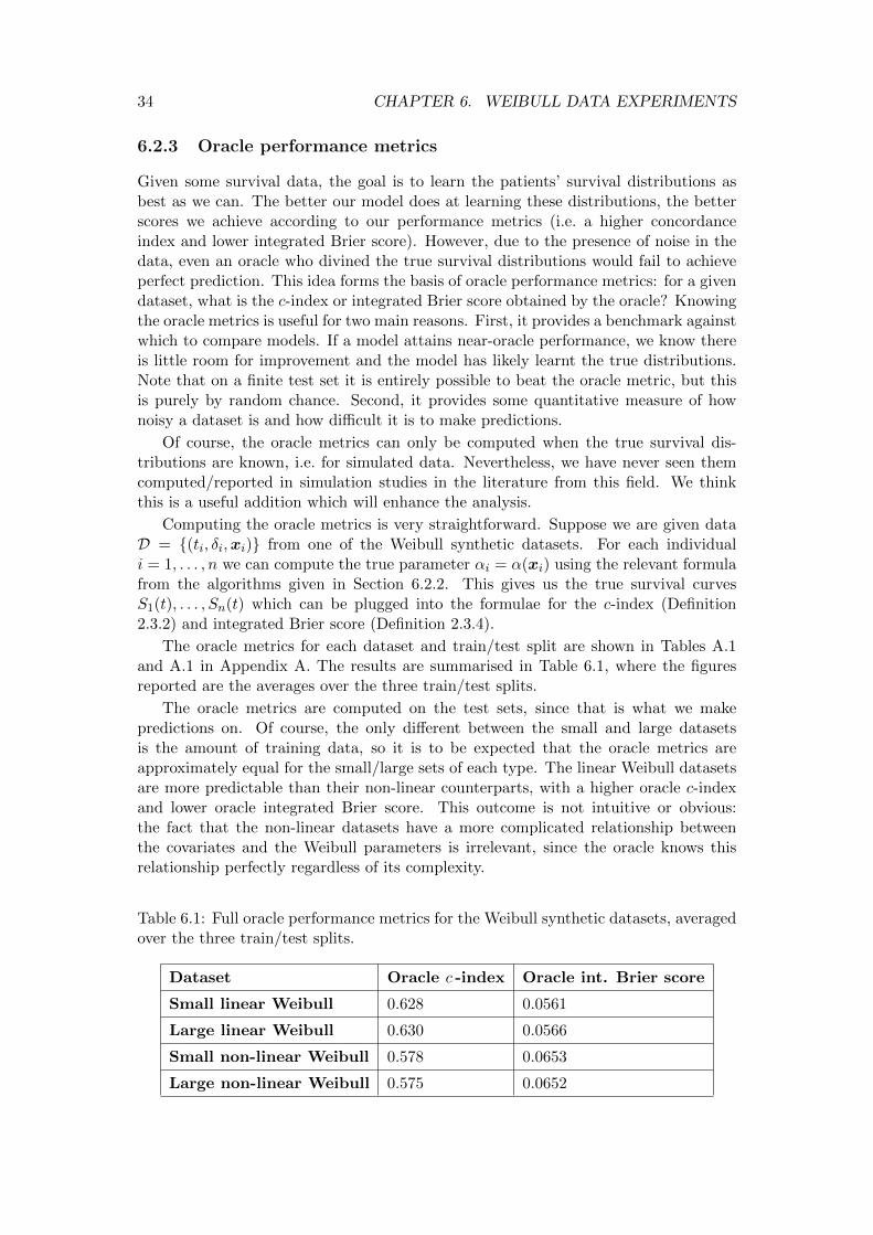
34 CHAPTER 6. WEIBULL DATA EXPERIMENTS
6.2.3 Oracle performance metrics
Given some survival data, the goal is to learn the patients’ survival distributions asbest as we can. The better our model does at learning these distributions, the betterscores we achieve according to our performance metrics (i.e. a higher concordanceindex and lower integrated Brier score). However, due to the presence of noise in thedata, even an oracle who divined the true survival distributions would fail to achieveperfect prediction. This idea forms the basis of oracle performance metrics: for a givendataset, what is the c-index or integrated Brier score obtained by the oracle? Knowingthe oracle metrics is useful for two main reasons. First, it provides a benchmark againstwhich to compare models. If a model attains near-oracle performance, we know thereis little room for improvement and the model has likely learnt the true distributions.Note that on a finite test set it is entirely possible to beat the oracle metric, but thisis purely by random chance. Second, it provides some quantitative measure of hownoisy a dataset is and how difficult it is to make predictions.
Of course, the oracle metrics can only be computed when the true survival dis-tributions are known, i.e. for simulated data. Nevertheless, we have never seen themcomputed/reported in simulation studies in the literature from this field. We thinkthis is a useful addition which will enhance the analysis.
Computing the oracle metrics is very straightforward. Suppose we are given dataD = {(ti, δi,xi)} from one of the Weibull synthetic datasets. For each individuali = 1, . . . , n we can compute the true parameter αi = α(xi) using the relevant formulafrom the algorithms given in Section 6.2.2. This gives us the true survival curvesS1(t), . . . , Sn(t) which can be plugged into the formulae for the c-index (Definition2.3.2) and integrated Brier score (Definition 2.3.4).
The oracle metrics for each dataset and train/test split are shown in Tables A.1and A.1 in Appendix A. The results are summarised in Table 6.1, where the figuresreported are the averages over the three train/test splits.
The oracle metrics are computed on the test sets, since that is what we makepredictions on. Of course, the only different between the small and large datasetsis the amount of training data, so it is to be expected that the oracle metrics areapproximately equal for the small/large sets of each type. The linear Weibull datasetsare more predictable than their non-linear counterparts, with a higher oracle c-indexand lower oracle integrated Brier score. This outcome is not intuitive or obvious:the fact that the non-linear datasets have a more complicated relationship betweenthe covariates and the Weibull parameters is irrelevant, since the oracle knows thisrelationship perfectly regardless of its complexity.
Table 6.1: Full oracle performance metrics for the Weibull synthetic datasets, averagedover the three train/test splits.
Dataset Oracle c -index Oracle int. Brier score
Small linear Weibull 0.628 0.0561
Large linear Weibull 0.630 0.0566
Small non-linear Weibull 0.578 0.0653
Large non-linear Weibull 0.575 0.0652
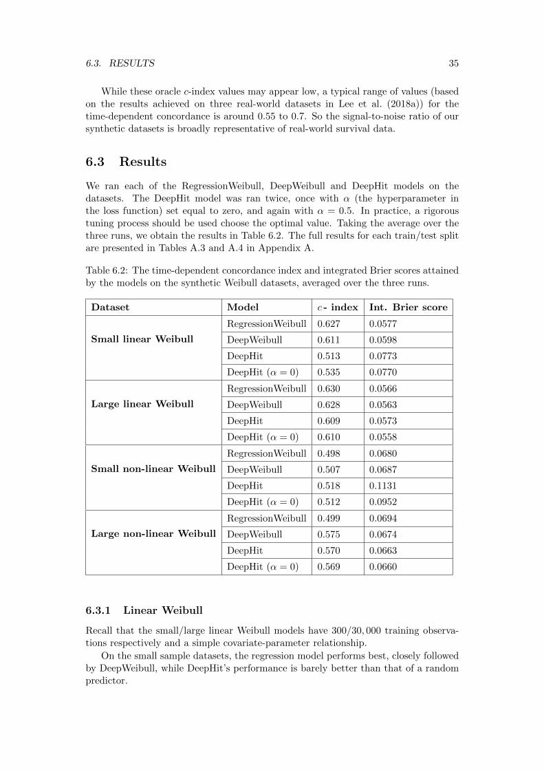
6.3. RESULTS 35
While these oracle c-index values may appear low, a typical range of values (basedon the results achieved on three real-world datasets in Lee et al. (2018a)) for thetime-dependent concordance is around 0.55 to 0.7. So the signal-to-noise ratio of oursynthetic datasets is broadly representative of real-world survival data.
6.3 Results
We ran each of the RegressionWeibull, DeepWeibull and DeepHit models on thedatasets. The DeepHit model was ran twice, once with α (the hyperparameter inthe loss function) set equal to zero, and again with α = 0.5. In practice, a rigoroustuning process should be used choose the optimal value. Taking the average over thethree runs, we obtain the results in Table 6.2. The full results for each train/test splitare presented in Tables A.3 and A.4 in Appendix A.
Table 6.2: The time-dependent concordance index and integrated Brier scores attainedby the models on the synthetic Weibull datasets, averaged over the three runs.
Dataset Model c - index Int. Brier score
Small linear Weibull
RegressionWeibull 0.627 0.0577
DeepWeibull 0.611 0.0598
DeepHit 0.513 0.0773
DeepHit (α = 0) 0.535 0.0770
Large linear Weibull
RegressionWeibull 0.630 0.0566
DeepWeibull 0.628 0.0563
DeepHit 0.609 0.0573
DeepHit (α = 0) 0.610 0.0558
Small non-linear Weibull
RegressionWeibull 0.498 0.0680
DeepWeibull 0.507 0.0687
DeepHit 0.518 0.1131
DeepHit (α = 0) 0.512 0.0952
Large non-linear Weibull
RegressionWeibull 0.499 0.0694
DeepWeibull 0.575 0.0674
DeepHit 0.570 0.0663
DeepHit (α = 0) 0.569 0.0660
6.3.1 Linear Weibull
Recall that the small/large linear Weibull models have 300/30, 000 training observa-tions respectively and a simple covariate-parameter relationship.
On the small sample datasets, the regression model performs best, closely followedby DeepWeibull, while DeepHit’s performance is barely better than that of a randompredictor.
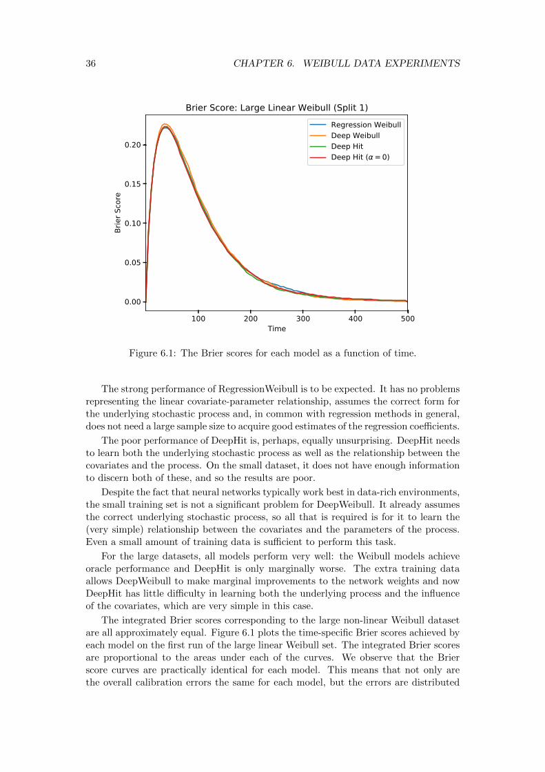
36 CHAPTER 6. WEIBULL DATA EXPERIMENTS
100 200 300 400 500Time
0.00
0.05
0.10
0.15
0.20
Brie
r Sco
reBrier Score: Large Linear Weibull (Split 1)
Regression WeibullDeep WeibullDeep HitDeep Hit ( = 0)
Figure 6.1: The Brier scores for each model as a function of time.
The strong performance of RegressionWeibull is to be expected. It has no problemsrepresenting the linear covariate-parameter relationship, assumes the correct form forthe underlying stochastic process and, in common with regression methods in general,does not need a large sample size to acquire good estimates of the regression coefficients.
The poor performance of DeepHit is, perhaps, equally unsurprising. DeepHit needsto learn both the underlying stochastic process as well as the relationship between thecovariates and the process. On the small dataset, it does not have enough informationto discern both of these, and so the results are poor.
Despite the fact that neural networks typically work best in data-rich environments,the small training set is not a significant problem for DeepWeibull. It already assumesthe correct underlying stochastic process, so all that is required is for it to learn the(very simple) relationship between the covariates and the parameters of the process.Even a small amount of training data is sufficient to perform this task.
For the large datasets, all models perform very well: the Weibull models achieveoracle performance and DeepHit is only marginally worse. The extra training dataallows DeepWeibull to make marginal improvements to the network weights and nowDeepHit has little difficulty in learning both the underlying process and the influenceof the covariates, which are very simple in this case.
The integrated Brier scores corresponding to the large non-linear Weibull datasetare all approximately equal. Figure 6.1 plots the time-specific Brier scores achieved byeach model on the first run of the large linear Weibull set. The integrated Brier scoresare proportional to the areas under each of the curves. We observe that the Brierscore curves are practically identical for each model. This means that not only arethe overall calibration errors the same for each model, but the errors are distributed
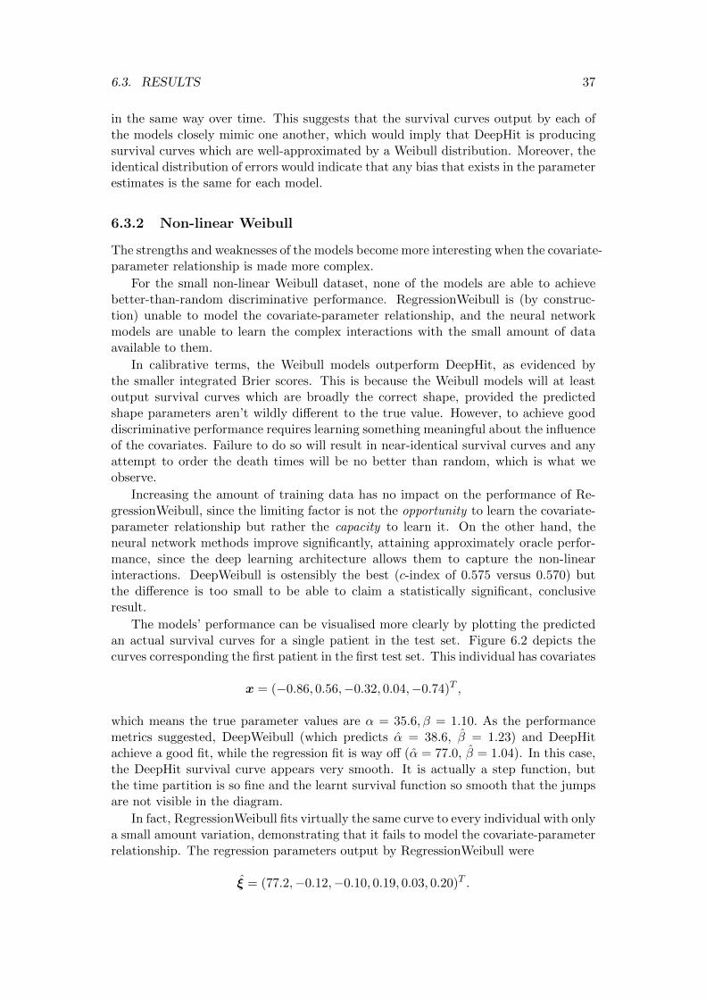
6.3. RESULTS 37
in the same way over time. This suggests that the survival curves output by each ofthe models closely mimic one another, which would imply that DeepHit is producingsurvival curves which are well-approximated by a Weibull distribution. Moreover, theidentical distribution of errors would indicate that any bias that exists in the parameterestimates is the same for each model.
6.3.2 Non-linear Weibull
The strengths and weaknesses of the models become more interesting when the covariate-parameter relationship is made more complex.
For the small non-linear Weibull dataset, none of the models are able to achievebetter-than-random discriminative performance. RegressionWeibull is (by construc-tion) unable to model the covariate-parameter relationship, and the neural networkmodels are unable to learn the complex interactions with the small amount of dataavailable to them.
In calibrative terms, the Weibull models outperform DeepHit, as evidenced bythe smaller integrated Brier scores. This is because the Weibull models will at leastoutput survival curves which are broadly the correct shape, provided the predictedshape parameters aren’t wildly different to the true value. However, to achieve gooddiscriminative performance requires learning something meaningful about the influenceof the covariates. Failure to do so will result in near-identical survival curves and anyattempt to order the death times will be no better than random, which is what weobserve.
Increasing the amount of training data has no impact on the performance of Re-gressionWeibull, since the limiting factor is not the opportunity to learn the covariate-parameter relationship but rather the capacity to learn it. On the other hand, theneural network methods improve significantly, attaining approximately oracle perfor-mance, since the deep learning architecture allows them to capture the non-linearinteractions. DeepWeibull is ostensibly the best (c-index of 0.575 versus 0.570) butthe difference is too small to be able to claim a statistically significant, conclusiveresult.
The models’ performance can be visualised more clearly by plotting the predictedan actual survival curves for a single patient in the test set. Figure 6.2 depicts thecurves corresponding the first patient in the first test set. This individual has covariates
x = (−0.86, 0.56,−0.32, 0.04,−0.74)T ,
which means the true parameter values are α = 35.6, β = 1.10. As the performancemetrics suggested, DeepWeibull (which predicts α = 38.6, β = 1.23) and DeepHitachieve a good fit, while the regression fit is way off (α = 77.0, β = 1.04). In this case,the DeepHit survival curve appears very smooth. It is actually a step function, butthe time partition is so fine and the learnt survival function so smooth that the jumpsare not visible in the diagram.
In fact, RegressionWeibull fits virtually the same curve to every individual with onlya small amount variation, demonstrating that it fails to model the covariate-parameterrelationship. The regression parameters output by RegressionWeibull were
ξ = (77.2,−0.12,−0.10, 0.19, 0.03, 0.20)T .
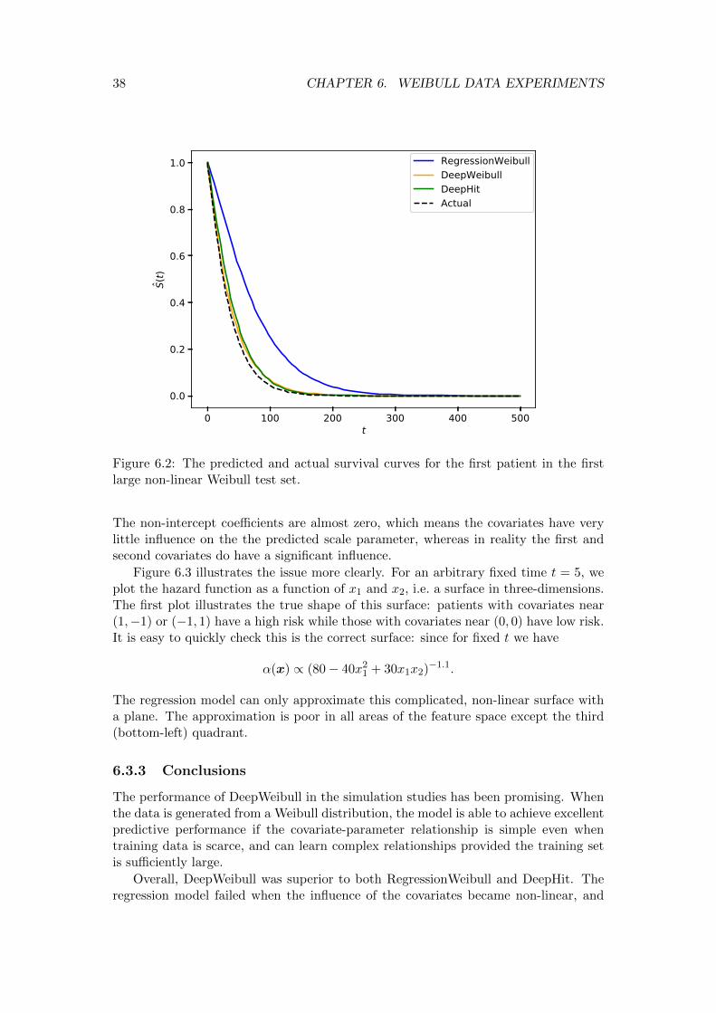
38 CHAPTER 6. WEIBULL DATA EXPERIMENTS
0 100 200 300 400 500t
0.0
0.2
0.4
0.6
0.8
1.0S(
t)RegressionWeibullDeepWeibullDeepHitActual
Figure 6.2: The predicted and actual survival curves for the first patient in the firstlarge non-linear Weibull test set.
The non-intercept coefficients are almost zero, which means the covariates have verylittle influence on the the predicted scale parameter, whereas in reality the first andsecond covariates do have a significant influence.
Figure 6.3 illustrates the issue more clearly. For an arbitrary fixed time t = 5, weplot the hazard function as a function of x1 and x2, i.e. a surface in three-dimensions.The first plot illustrates the true shape of this surface: patients with covariates near(1,−1) or (−1, 1) have a high risk while those with covariates near (0, 0) have low risk.It is easy to quickly check this is the correct surface: since for fixed t we have
α(x) ∝ (80− 40x21 + 30x1x2)−1.1.
The regression model can only approximate this complicated, non-linear surface witha plane. The approximation is poor in all areas of the feature space except the third(bottom-left) quadrant.
6.3.3 Conclusions
The performance of DeepWeibull in the simulation studies has been promising. Whenthe data is generated from a Weibull distribution, the model is able to achieve excellentpredictive performance if the covariate-parameter relationship is simple even whentraining data is scarce, and can learn complex relationships provided the training setis sufficiently large.
Overall, DeepWeibull was superior to both RegressionWeibull and DeepHit. Theregression model failed when the influence of the covariates became non-linear, and
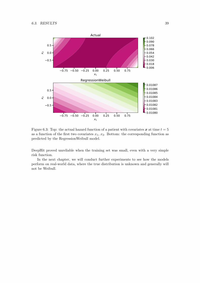
6.3. RESULTS 39
0.75 0.50 0.25 0.00 0.25 0.50 0.75x1
0.5
0.0
0.5x 2
Actual
0.75 0.50 0.25 0.00 0.25 0.50 0.75x1
0.5
0.0
0.5
x 2
RegressionWeibull
0.0060.0180.0300.0420.0540.0660.0780.0900.102
0.010800.010810.010820.010830.010840.010850.010860.01087
Figure 6.3: Top: the actual hazard function of a patient with covariates x at time t = 5as a function of the first two covariates x1, x2. Bottom: the corresponding function aspredicted by the RegressionWeibull model.
DeepHit proved unreliable when the training set was small, even with a very simplerisk function.
In the next chapter, we will conduct further experiments to see how the modelsperform on real-world data, where the true distribution is unknown and generally willnot be Weibull.
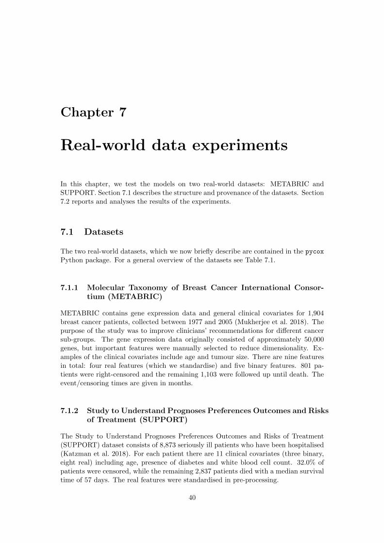
Chapter 7
Real-world data experiments
In this chapter, we test the models on two real-world datasets: METABRIC andSUPPORT. Section 7.1 describes the structure and provenance of the datasets. Section7.2 reports and analyses the results of the experiments.
7.1 Datasets
The two real-world datasets, which we now briefly describe are contained in the pycox
Python package. For a general overview of the datasets see Table 7.1.
7.1.1 Molecular Taxonomy of Breast Cancer International Consor-tium (METABRIC)
METABRIC contains gene expression data and general clinical covariates for 1,904breast cancer patients, collected between 1977 and 2005 (Mukherjee et al. 2018). Thepurpose of the study was to improve clinicians’ recommendations for different cancersub-groups. The gene expression data originally consisted of approximately 50,000genes, but important features were manually selected to reduce dimensionality. Ex-amples of the clinical covariates include age and tumour size. There are nine featuresin total: four real features (which we standardise) and five binary features. 801 pa-tients were right-censored and the remaining 1,103 were followed up until death. Theevent/censoring times are given in months.
7.1.2 Study to Understand Prognoses Preferences Outcomes and Risksof Treatment (SUPPORT)
The Study to Understand Prognoses Preferences Outcomes and Risks of Treatment(SUPPORT) dataset consists of 8,873 seriously ill patients who have been hospitalised(Katzman et al. 2018). For each patient there are 11 clinical covariates (three binary,eight real) including age, presence of diabetes and white blood cell count. 32.0% ofpatients were censored, while the remaining 2,837 patients died with a median survivaltime of 57 days. The real features were standardised in pre-processing.
40
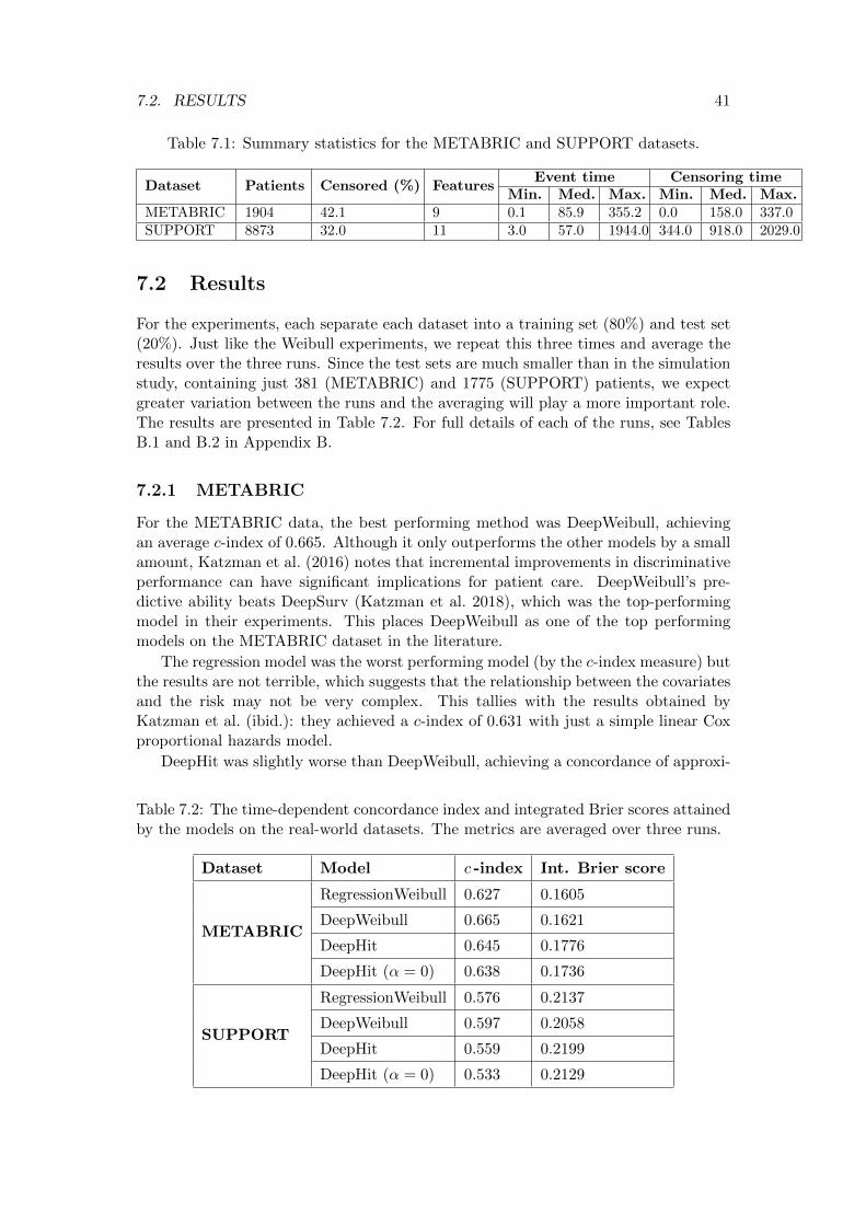
7.2. RESULTS 41
Table 7.1: Summary statistics for the METABRIC and SUPPORT datasets.
Dataset Patients Censored (%) FeaturesEvent time Censoring time
Min. Med. Max. Min. Med. Max.METABRIC 1904 42.1 9 0.1 85.9 355.2 0.0 158.0 337.0SUPPORT 8873 32.0 11 3.0 57.0 1944.0 344.0 918.0 2029.0
7.2 Results
For the experiments, each separate each dataset into a training set (80%) and test set(20%). Just like the Weibull experiments, we repeat this three times and average theresults over the three runs. Since the test sets are much smaller than in the simulationstudy, containing just 381 (METABRIC) and 1775 (SUPPORT) patients, we expectgreater variation between the runs and the averaging will play a more important role.The results are presented in Table 7.2. For full details of each of the runs, see TablesB.1 and B.2 in Appendix B.
7.2.1 METABRIC
For the METABRIC data, the best performing method was DeepWeibull, achievingan average c-index of 0.665. Although it only outperforms the other models by a smallamount, Katzman et al. (2016) notes that incremental improvements in discriminativeperformance can have significant implications for patient care. DeepWeibull’s pre-dictive ability beats DeepSurv (Katzman et al. 2018), which was the top-performingmodel in their experiments. This places DeepWeibull as one of the top performingmodels on the METABRIC dataset in the literature.
The regression model was the worst performing model (by the c-index measure) butthe results are not terrible, which suggests that the relationship between the covariatesand the risk may not be very complex. This tallies with the results obtained byKatzman et al. (ibid.): they achieved a c-index of 0.631 with just a simple linear Coxproportional hazards model.
DeepHit was slightly worse than DeepWeibull, achieving a concordance of approxi-
Table 7.2: The time-dependent concordance index and integrated Brier scores attainedby the models on the real-world datasets. The metrics are averaged over three runs.
Dataset Model c -index Int. Brier score
METABRIC
RegressionWeibull 0.627 0.1605
DeepWeibull 0.665 0.1621
DeepHit 0.645 0.1776
DeepHit (α = 0) 0.638 0.1736
SUPPORT
RegressionWeibull 0.576 0.2137
DeepWeibull 0.597 0.2058
DeepHit 0.559 0.2199
DeepHit (α = 0) 0.533 0.2129
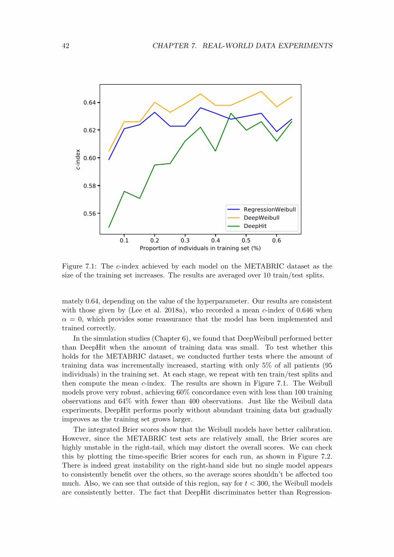
42 CHAPTER 7. REAL-WORLD DATA EXPERIMENTS
0.1 0.2 0.3 0.4 0.5 0.6Proportion of individuals in training set (%)
0.56
0.58
0.60
0.62
0.64
c-in
dex
RegressionWeibullDeepWeibullDeepHit
Figure 7.1: The c-index achieved by each model on the METABRIC dataset as thesize of the training set increases. The results are averaged over 10 train/test splits.
mately 0.64, depending on the value of the hyperparameter. Our results are consistentwith those given by (Lee et al. 2018a), who recorded a mean c-index of 0.646 whenα = 0, which provides some reassurance that the model has been implemented andtrained correctly.
In the simulation studies (Chapter 6), we found that DeepWeibull performed betterthan DeepHit when the amount of training data was small. To test whether thisholds for the METABRIC dataset, we conducted further tests where the amount oftraining data was incrementally increased, starting with only 5% of all patients (95individuals) in the training set. At each stage, we repeat with ten train/test splits andthen compute the mean c-index. The results are shown in Figure 7.1. The Weibullmodels prove very robust, achieving 60% concordance even with less than 100 trainingobservations and 64% with fewer than 400 observations. Just like the Weibull dataexperiments, DeepHit performs poorly without abundant training data but graduallyimproves as the training set grows larger.
The integrated Brier scores show that the Weibull models have better calibration.However, since the METABRIC test sets are relatively small, the Brier scores arehighly unstable in the right-tail, which may distort the overall scores. We can checkthis by plotting the time-specific Brier scores for each run, as shown in Figure 7.2.There is indeed great instability on the right-hand side but no single model appearsto consistently benefit over the others, so the average scores shouldn’t be affected toomuch. Also, we can see that outside of this region, say for t < 300, the Weibull modelsare consistently better. The fact that DeepHit discriminates better than Regression-
7.2. RESULTS 43
Weibull but has worse calibration suggest it has done a better job at learning howcovariates affect risk, but the shape of the predicted survival curves is not as accurate.
7.2.2 SUPPORT
SUPPORT was not among the datasets tested by Lee et al. (ibid.) but was used byKatzman et al. (2018). In their experiments, the top performing algorithm achieved aconcordance index of 0.619. None of the models in our experiments were able to beatthis, with the top-performer, DeepWeibull, achieving 0.597. However, in the DeepSurvexperiments the model hyperparameters such as the number of layers, nodes per layerand the dropout rate, were optimised by random search for each dataset, while they arefixed for DeepWeibull and DeepHit, e.g. there are three hidden layers and the widthsare set multiples of the number of features. Our approach means the models can beused ’off-the-shelf’, which may be useful for clinicians who do not have the technicalexpertise to optimise deep learning models, but means performance is potentially sub-optimal. Bearing this difference in methodology in mind, we can be more optimisticabout how DeepWeibull fared on the SUPPORT dataset.
Again, the performance of the regression model is comparable to that achievedby the Cox proportional hazards model (0.583) in the DeepSurv experiments. Thesimilarity in the performance between the Cox and Weibull regression models is to beexpected: experiments by Crumer (2017) found that this tends to be the case.
Somewhat surprisingly, DeepHit performs very poorly on this dataset. The problemis illustrated in Figure 7.3, which shows the survival curves predicted by each modelfor the first 20 patients in the first SUPPORT test set. The Weibull models outputsurvival curves which are fairly distinct from one another have a clear ordering, whilethe DeepHit survival curves are tightly clustered and frequently intersect one another.The fact that the survival curves intersect is not an issue per se, the time-dependentconcordance index was developed to deal with this, but in this case it is clear that themodel has been unable to make any significant progress with risk stratification. Evensetting the hyperparameter α to a very large value led to no significant improvementin the concordance.
The SUPPORT dataset provides a nice example of the interpretability of theWeibull model. We find that the shape parameters predicted by the Weibull mod-els are all comfortably below 1, which indicates a decreasing hazard rate. This seemsreasonable for seriously ill hospitalised patients, though clearly this will vary dependingon the nature of the disease.
7.2.3 Conclusions
DeepWeibull performed strongly on both of the real-world datasets, and was superiorto RegressionWeibull and DeepHit in both cases. On the METABRIC dataset, it rivalsthe performance of top-performing models in the literature, and even performs wellwith a limited amount of training data. Performance on the SUPPORT dataset wasrespectable, but not as good as some existing models, with the caveat that said modelswere specifically optimised for the dataset in question.
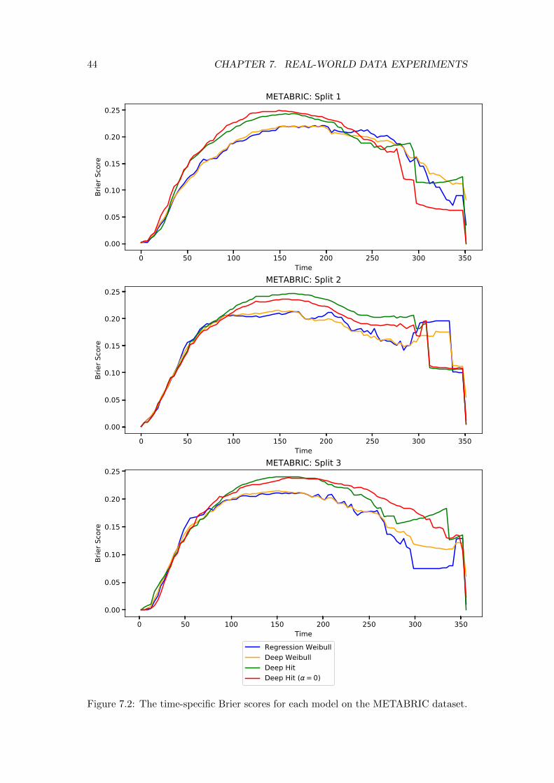
44 CHAPTER 7. REAL-WORLD DATA EXPERIMENTS
0 50 100 150 200 250 300 350Time
0.00
0.05
0.10
0.15
0.20
0.25Br
ier S
core
METABRIC: Split 1
0 50 100 150 200 250 300 350Time
0.00
0.05
0.10
0.15
0.20
0.25
Brie
r Sco
re
METABRIC: Split 2
0 50 100 150 200 250 300 350Time
0.00
0.05
0.10
0.15
0.20
0.25
Brie
r Sco
re
METABRIC: Split 3
Regression WeibullDeep WeibullDeep HitDeep Hit ( = 0)
Figure 7.2: The time-specific Brier scores for each model on the METABRIC dataset.
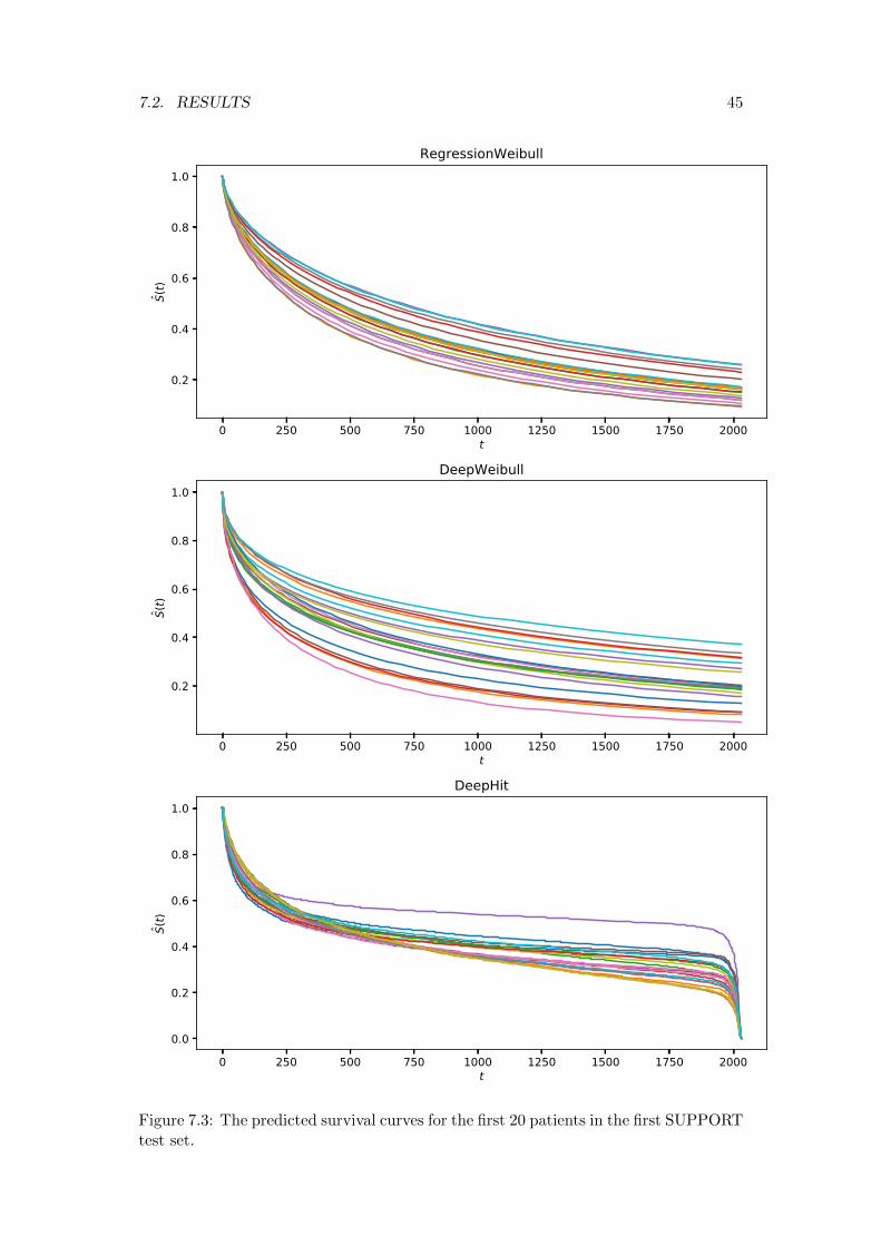
7.2. RESULTS 45
0 250 500 750 1000 1250 1500 1750 2000t
0.2
0.4
0.6
0.8
1.0S(
t)RegressionWeibull
0 250 500 750 1000 1250 1500 1750 2000t
0.2
0.4
0.6
0.8
1.0
S(t)
DeepWeibull
0 250 500 750 1000 1250 1500 1750 2000t
0.0
0.2
0.4
0.6
0.8
1.0
S(t)
DeepHit
Figure 7.3: The predicted survival curves for the first 20 patients in the first SUPPORTtest set.
Chapter 8
Discussion
This chapter serves to conclude the thesis. Some directions for future research aresuggested in Section 8.1. Finally, we briefly discuss relevant ethical considerations withreference to the ESPRC’s framework for responsible innovation. Section 8.3 recaps thekey findings of the thesis.
8.1 Future work
Other parametric distributions: A straightforward extension to the tests con-ducted in this thesis would be to implement models based on other parametricdistributions, such as the exponential, Gamma or Gompertz-Makeham distribu-tions.
Confidence bands: The output of DeepWeibull is a point prediction of the sur-vival curve. It would be useful if we could gauge the error in this point estimate, i.e.obtain something analogous to the Greenwood formula for the Kaplan-Meier esti-mate, which can be used to construct pointwise confidence intervals. One possibleapproach might be to use Bayesian neural networks, where a probability distribu-tion is attached to the network weights and the outputs are probability distributionsfor the Weibull parameters.
Competing risks: Unlike DeepHit, the proposed model can only handle single-event survival data. Baghestani and Hosseini-Baharanchi (2019) have shown howthe Weibull parametric model can be extended to incorporate a competing risksframework. It would be interesting to see if the DeepWeibull model can be adaptedto implement their approach.
Comparisons with more models: Lots of new approaches have been developedin this area. It would be useful to run comparisons with more of these models,including non neural network models. DeepSurv and RSF (Ishwaran et al. 2008)regularly feature as top-performing models in the literature, so these would benatural candidates. In this thesis, we have relied upon accepting the results ofother researchers in our comparisons.
Work with Gumbel and log-times: Instead of using the Weibull distribution,we could have proceeded in a similar way to Weibull regression models by working
46
8.2. ETHICAL CONSIDERATIONS 47
with log-transformed event times and learn the parameters of the Gumbel distri-bution. In the first instance, there was no need to do this, since we can ensurethe model outputs a valid survival model by choosing the appropriate activationfunction for the output layer. It would be interesting to test whether this approachwould yield better results.
Test on highly-censored data: Our tests did involve some ’stress-testing’, e.g.using a small amount of training data, but we could go further. In particular, wecould see what happens when the censoring fraction is very high. From the workin Section 5.2.3, we expect stability issues and exploding gradients. Aspects of thenetwork configuration and training process may require some revision to cope withsuch data.
8.2 Ethical considerations
The ESPRC outlines a ’Responsible Innovation’ approach, which promotes consider-ation of the ethical and social impact of research (Stilgoe, Owen, and Macnaghten2013). Guided by this framework, in this section we will briefly discuss the ethicalconsideration relating to this thesis.
DeepWeibull is a general purpose survival model. The datasets used as exampleshave been related to applications in medicine, but the model could conceivably beused in a wide variety of fields. It is not possible to anticipate all the possible areas ofapplication.
Underpinning the DeepWeibull model are certain assumptions. The most impor-tant is the parametric assumption. Further assumptions are also in-built, e.g. thatobservations are independent and censoring is independent and non-informative. Inscenarios where these assumptions are clearly violated (e.g. the hazard function ismultimodal), the model cannot be expected to work reliably, and alternative modelsshould be preferred.
In common with other machine learning models, DeepWeibull may be unreliableif only a small amount of training data is available, particularly if the risk function iscomplex. The model should be used with great caution in circumstances where thereare few training observations. Indeed, before applying the model to new data, theuser should undertake some validation steps to ensure the model works properly. Themodel should only be used to predict the outcomes of patients whose covariates aresimilar to those used in the training process.
The output of the model is a point prediction of the survival curves, i.e. for eachpatient we obtain one survival curve with no confidence bands. The user is able tomake statements of the form ”patient X has an estimated probability p of survivingpast time t”, but the error in the value of p is unknown. This limitation may haveethical implications in some contexts: e.g. a patient being denied treatment based ontheir survival prospects narrowly failing to meet a minimum threshold.
8.3 Summary and conclusions
The goal of this thesis was to propose a deep learning approach to survival analy-sis which complements or improves upon previous approaches. The proposed model,
48 CHAPTER 8. DISCUSSION
DeepWeibull, uses a deep neural network to fit a Weibull distribution and is trainedusing a loss function based on the log-likelihood for censored data.
The motivation behind the model is multifaceted. First, the Weibull model is apopular survival model with some useful properties (e.g. the weakest link property) anddeveloping a neural network extension seems a logical next step. Second, it fits nicelywithin the existing suite of neural network survival models, by imposing assumptionson the underlying stochastic process but not on the relationship between the covariatesand the parameters of the process. Previous approaches tend to impose restrictionson both of these elements, or on neither.
The results from the experiments were very promising. On the simulated datasets,the model was able to attain oracle-level performance and coped well with both smalland large training sets. For the METABRIC dataset, DeepWeibull attained perfor-mance which rivals the top-performing models in the literature and maintained excel-lent predictive capabilities even when minimal training data was available. The resultsfor the SUPPORT dataset were respectable but failed to outperform some previousmodels; it still performed well in spite of our ’off-the-shelf’ approach, where the modelhyperparameters are pre-determined and not optimised for each dataset.
DeepWeibull, we conclude, has been shown to be applicable to real-world datasetsand offers a very simple yet high-performing alternative to existing models.
Bibliography
Antolini, L., P. Boracchi, and E. Biganzoli (2005). “A time-dependent discriminationindex for survival data”. In: Statistics in Medicine 24.24, pp. 3827–3944.doi: 10.1002/sim.2427.
Baghestani, A. and F. Hosseini-Baharanchi (2019). “An improper form of Weibulldistribution for competing risks analysis with Bayesian approach”. In: Journal ofApplied Statistics 46.13, pp. 2409–2417.doi: 10.1080/02664763.2019.1597027.
Biganzoli, E. et al. (1998). “Feed forward neural networks for the analysis of censoredsurvival data: a partial logistic regression approach”. In: Statistics in Medicine17.10, pp. 1169–1186.doi: 10.1002/(SICI)1097-0258(19980530)17:10<1169::AID-SIM796>3.0.CO;2-D.
Box-Steffensmeier, J. and S. Jones (2004). Event History Modeling: A Guide for SocialScientists. Cambridge University Press. isbn: 9780521546737.
Brier, G. W. (1950). “Verification of forecasts expressed in terms of probability”. In:Monthly Weather Review 78.1, pp. 1–3.doi: 10.1175/1520-0493(1950)078<0001:VOFEIT>2.0.CO;2.
Casella, G. and R. L. Berger (2002). Statistical Inference. Second. Thomson Learning.
Cox, D. R. (1972). “Regression Models and Life-Tables”. In: Journal of the RoyalStatistical Society: Series B (Methodological) 34.2, pp. 187–202.doi: 10.1111/j.2517-6161.1972.tb00899.x.
Crumer, A. (2017). “Comparison between Weibull and Cox Proportional Hazards Mod-els”. MA thesis. Southeast Missouri State University.url:
Faraggi, S. and R. Simon (1995). “A neural network model for survival data”. In:Statistics in Medicine 14.1, pp. 73–82.doi: 10.1002/sim.4780140108.
Fine, J. P. and R. J. Gray (1999). “A Proportional Hazards Model for the Subdistri-bution of a Competing Risk”. In: Journal of the American Statistical Association
49
50 BIBLIOGRAPHY
94.446, pp. 496–509.doi: 10.1080/01621459.1999.10474144.
Haan, L. de and A. Ferreira (2006). Extreme Value Theory: An Introduction. First.Springer New York.doi: 10.1007/0-387-34471-3.
Haller, B., G. Schmidt, and K. Ulm (2013). “Applying competing risks regressionmodels: an overview”. In: Lifetime Data Analysis 19.1, pp. 33–58.doi: 10.1007/s10985-012-9230-8.
Hastie, T., R. Tibshirani, and J. Friedman (2009). The Elements of Statistical Learning:Data Mining, Inference and Prediction. Second. Springer New York.doi: 10.1007/978-0-387-84858-7.
Ishwaran, H. et al. (2008). “Random survival forests”. In: The Annals of Applied Statis-tics 2.3, pp. 841–860.doi: 10.1214/08-AOAS169.
Janocha, K. and W. Czarnecki (2016). “On loss functions for deep neural networks inclassification”. In: Schedae Informaticae 25.1, pp. 49–59.doi: 10.4467/20838476SI.16.004.6185.
Katzman, J. L. et al. (2016). DeepSurv: Personalized Treatment Recommender SystemUsing A Deep Cox Proportional Hazards Network.doi: 10.1186/s12874-018-0482-1.
— (2018). “DeepSurv: personalised treatment recommender system using a Cox pro-portional hazards deep neural network”. In: BMC Medical Research Methodology18.1, pp. 1–12.doi: 10.1186/s12874-018-0482-1.
Kleinbaum, D. G. and M. Klein (2012). Survival Analysis. Third. Springer-Verlag NewYork.doi: 10.1007/978-1-4419-6646-9.
Kvamme, H. and Ø. Borgan (2019). The Brier Score under Administrative Censoring:Problems and Solutions.
Kvamme, H., Ø. Borgan, and I. Scheel (2019). “Time-to-Event Prediction with NeuralNetworks and Cox Regressions”. In: Journal of Machine Learning Research 20.129,pp. 1–30.
Lee, C. et al. (2018a). “DeepHit: A Deep Learning Approach to Survival Analysis WithCompeting Risks”. In: AAAI Conference on Artificial Intelligence.
— (2018b). “Supplementary Materials for DeepHit: A Deep Learning Approach toSurvival Analysis with Competing Risks”. In:
BIBLIOGRAPHY 51
Leung, K. M., R. M. Elashoff, and A. A. Afifi (1997). “Censoring Issues in SurvivalAnalysis”. In: Annual Review of Public Health 18, pp. 83–104.doi: 10.1146/annurev.publhealth.18.1.83.
Liestøl, K., P. Kragh, and U. Andersen (1994). “Survival analysis and neural nets”.In: Statistics in Medicine 13.12, pp. 1189–1200.doi: 10.1002/sim.4780131202.
Martinsson, E. (2017). “WTTE-RNN: Weibull Time to Event Recurrent Neural Net-work”. MA thesis. University of Gothenburg.url:
Moore, D. F. (2016). Applied Survival Analysis using R. Springer International Pub-lishing.doi: 10.1007/978-3-319-31245-3.
Mukherjee, A. et al. (2018). “Associations between genomic stratification of breastcancer and centrally reviewed tumour pathology in the METABRIC cohort”. In:NPJ Breast Cancer 4.1, p. 5.doi: 10.1038/s41523-018-0056-8.
Ng, S. K. et al. (2004). “Modelling the distribution of ischaemic stroke-specific survivaltime using an EM-based mixture approach with random effects adjustment”. In:Statistics in Medicine 23.17, pp. 2729–2744.doi: 10.1002/sim.1840.
Nwankpa, C. et al. (2018). Activation Functions: Comparison of Trends in Practiceand Research for Deep Learning.
Oirbeek, R. van, E. Lesaffre, and G. Molenberghs (2010). “An application of Harrell’sC-index to PH frailty models”. In: Statistics in Medicine 29.30, pp. 3160–3171.doi: 10.1002/sim.4058.
Prentice, R. L. and L. A. Gloeckler (1978). “Regression Analysis of Grouped SurvivalData with Application to Breast Cancer Data”. In: Biometrics 34.1, pp. 57–67.doi: 10.2307/2529588.
Raykar, V. C. et al. (2007). “On Ranking in Survival Analysis: Bounds on the Con-cordance Index”. In: Proceedings of the 20th International Conference on NeuralInformation Processing Systsme. Curran Associates Inc., pp. 1209–1216.doi: 10.5555/2981562.2981714.
Scholz, F. W. (1996). “Maximum likelihood estimation for type I censored Weibulldata including covariates”. In: ISSTECH-96-022.
— (2015). “Inference for the Weibull Distribution: A Tutorial”. In: Tutorials in Quan-titative Methods for Psychology 11.3, pp. 148–173.doi: 10.20982/tqmp.11.3.p148.
52 BIBLIOGRAPHY
Sibi, P., S. A. Jones, and P. Siddarth (2013). “Analysis of different activation functionsusing back propagation neural networks”. In: Journal of Theoretical and AppliedInformation Technology 47.3, pp. 1344–1348.
Steyerberg, E. W. (2019). Clinical Prediction Models: A Practical Approach to Devel-opment, Validation and Updating. Second. Springer International Publishing.doi: 10.1007/978-3-030-16399-0.
Stilgoe, J., R. Owen, and P. Macnaghten (2013). “Developing a framework for respon-sible innovation”. In: Research Policy 42.9, pp. 1568–1580.doi: 10.1016/j.respol.2013.05.008.
Wang, P., Y. Li, and C. Reddy (2019). “Machine learning for survival analysis: Asurvey”. In: ACM Computing Surveys 51.6, pp. 1–36.doi: 10.1145/3214306.
Xiang, A. et al. (2000). “Comparison of the performance of neural network methodsand Cox regression for censored survival data”. In: Computational Statistics andData Analysis 34.2, pp. 243–257.doi: 10.1016/S0167-9473(99)00098-5.
Xu, R. (2017). “Methods for Survival Analysis in Small Samples”. PhD thesis. Uni-versity of Pennsylvania.url:
Zhang, Y. et al. (2002). “Weibull analysis of the tensile behaviour of fibers with geo-metrical irregularities”. In: Journal of Materials Science 37.7, pp. 1401–1406.doi: 10.1023/A:1014580814803.
Zhao, L. and D. Feng (2020). “DNNSurv: Deep Neural Networks for Survival Analysisusing Pseudo Values”. In: IEEE Journal of Biomedical and Health Informatics [inpress].doi: 10.1109/JBHI.2020.2980204.
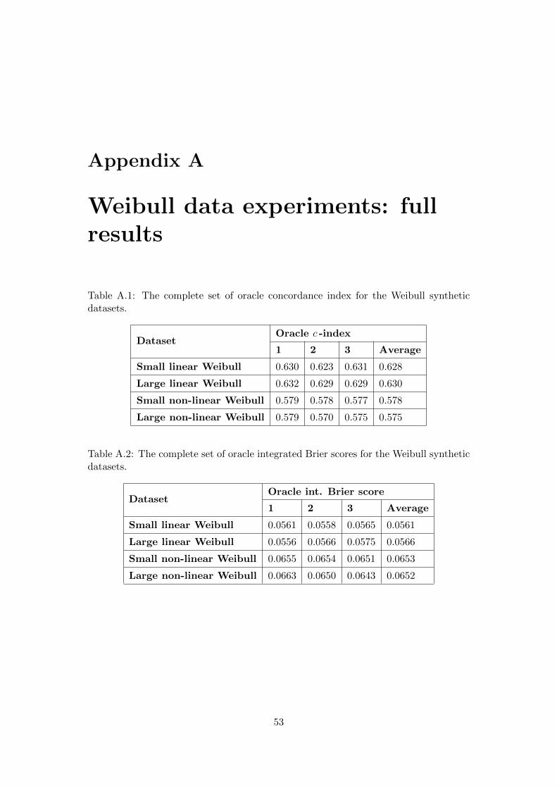
Appendix A
Weibull data experiments: fullresults
Table A.1: The complete set of oracle concordance index for the Weibull syntheticdatasets.
DatasetOracle c -index
1 2 3 Average
Small linear Weibull 0.630 0.623 0.631 0.628
Large linear Weibull 0.632 0.629 0.629 0.630
Small non-linear Weibull 0.579 0.578 0.577 0.578
Large non-linear Weibull 0.579 0.570 0.575 0.575
Table A.2: The complete set of oracle integrated Brier scores for the Weibull syntheticdatasets.
DatasetOracle int. Brier score
1 2 3 Average
Small linear Weibull 0.0561 0.0558 0.0565 0.0561
Large linear Weibull 0.0556 0.0566 0.0575 0.0566
Small non-linear Weibull 0.0655 0.0654 0.0651 0.0653
Large non-linear Weibull 0.0663 0.0650 0.0643 0.0652
53
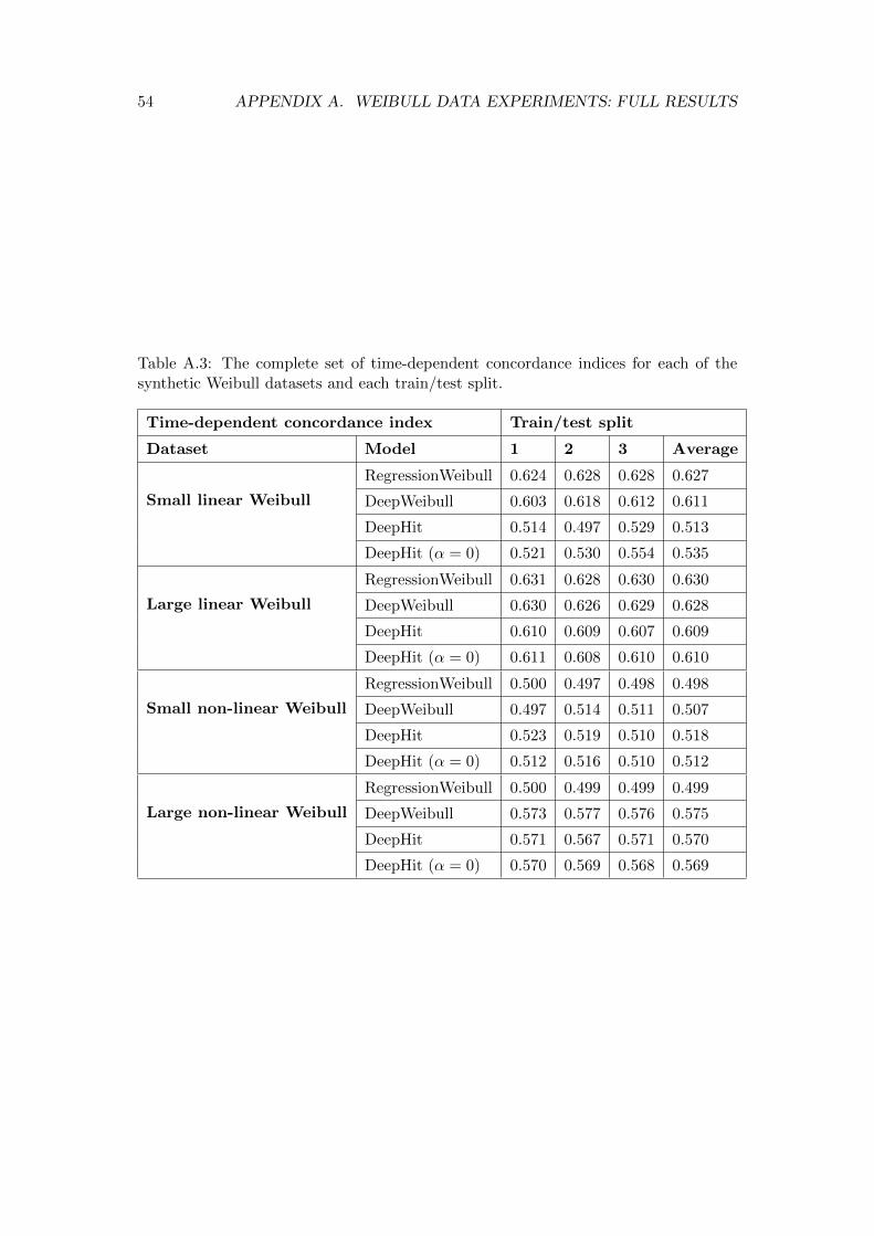
54 APPENDIX A. WEIBULL DATA EXPERIMENTS: FULL RESULTS
Table A.3: The complete set of time-dependent concordance indices for each of thesynthetic Weibull datasets and each train/test split.
Time-dependent concordance index Train/test split
Dataset Model 1 2 3 Average
Small linear Weibull
RegressionWeibull 0.624 0.628 0.628 0.627
DeepWeibull 0.603 0.618 0.612 0.611
DeepHit 0.514 0.497 0.529 0.513
DeepHit (α = 0) 0.521 0.530 0.554 0.535
Large linear Weibull
RegressionWeibull 0.631 0.628 0.630 0.630
DeepWeibull 0.630 0.626 0.629 0.628
DeepHit 0.610 0.609 0.607 0.609
DeepHit (α = 0) 0.611 0.608 0.610 0.610
Small non-linear Weibull
RegressionWeibull 0.500 0.497 0.498 0.498
DeepWeibull 0.497 0.514 0.511 0.507
DeepHit 0.523 0.519 0.510 0.518
DeepHit (α = 0) 0.512 0.516 0.510 0.512
Large non-linear Weibull
RegressionWeibull 0.500 0.499 0.499 0.499
DeepWeibull 0.573 0.577 0.576 0.575
DeepHit 0.571 0.567 0.571 0.570
DeepHit (α = 0) 0.570 0.569 0.568 0.569
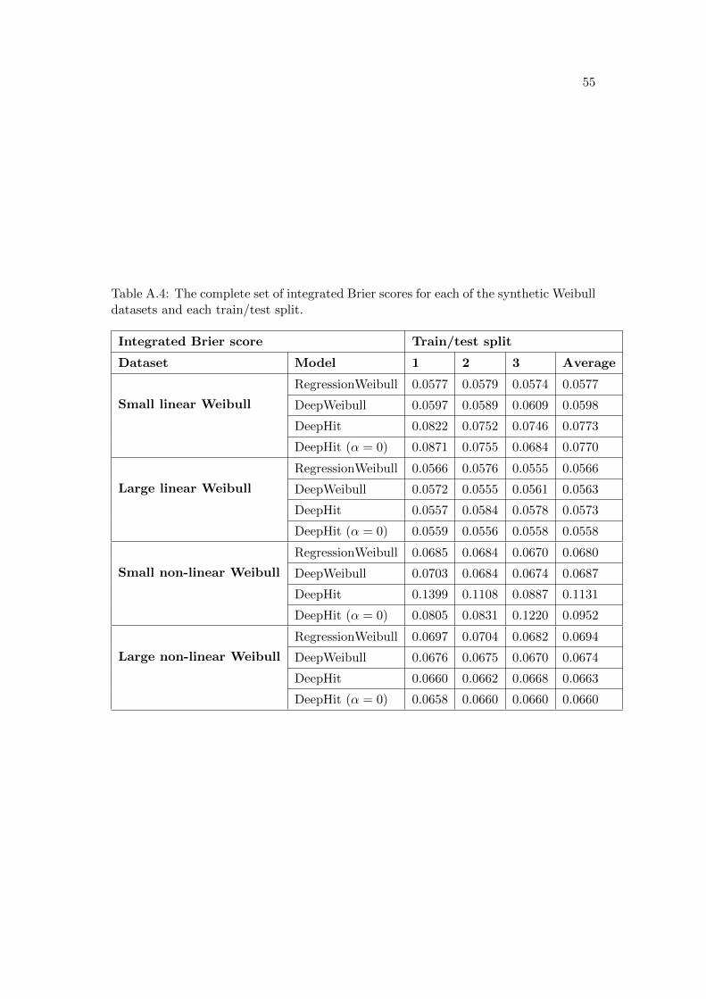
55
Table A.4: The complete set of integrated Brier scores for each of the synthetic Weibulldatasets and each train/test split.
Integrated Brier score Train/test split
Dataset Model 1 2 3 Average
Small linear Weibull
RegressionWeibull 0.0577 0.0579 0.0574 0.0577
DeepWeibull 0.0597 0.0589 0.0609 0.0598
DeepHit 0.0822 0.0752 0.0746 0.0773
DeepHit (α = 0) 0.0871 0.0755 0.0684 0.0770
Large linear Weibull
RegressionWeibull 0.0566 0.0576 0.0555 0.0566
DeepWeibull 0.0572 0.0555 0.0561 0.0563
DeepHit 0.0557 0.0584 0.0578 0.0573
DeepHit (α = 0) 0.0559 0.0556 0.0558 0.0558
Small non-linear Weibull
RegressionWeibull 0.0685 0.0684 0.0670 0.0680
DeepWeibull 0.0703 0.0684 0.0674 0.0687
DeepHit 0.1399 0.1108 0.0887 0.1131
DeepHit (α = 0) 0.0805 0.0831 0.1220 0.0952
Large non-linear Weibull
RegressionWeibull 0.0697 0.0704 0.0682 0.0694
DeepWeibull 0.0676 0.0675 0.0670 0.0674
DeepHit 0.0660 0.0662 0.0668 0.0663
DeepHit (α = 0) 0.0658 0.0660 0.0660 0.0660
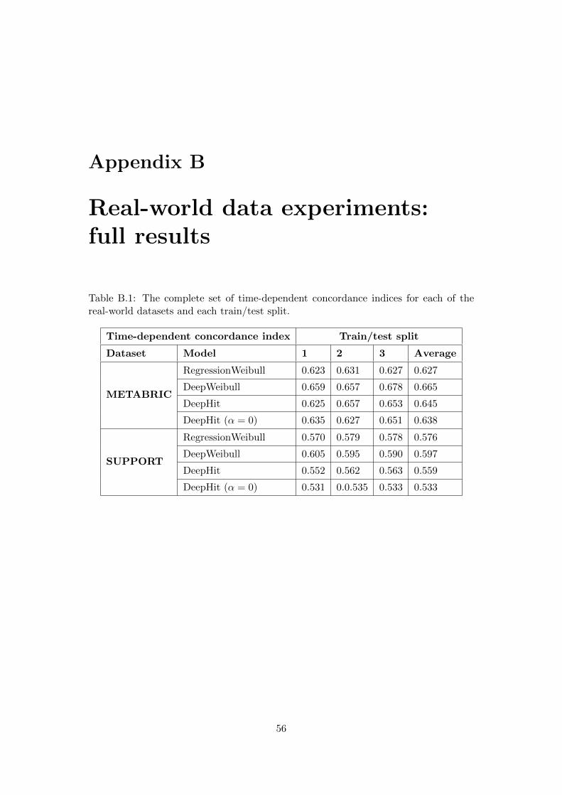
Appendix B
Real-world data experiments:full results
Table B.1: The complete set of time-dependent concordance indices for each of thereal-world datasets and each train/test split.
Time-dependent concordance index Train/test split
Dataset Model 1 2 3 Average
METABRIC
RegressionWeibull 0.623 0.631 0.627 0.627
DeepWeibull 0.659 0.657 0.678 0.665
DeepHit 0.625 0.657 0.653 0.645
DeepHit (α = 0) 0.635 0.627 0.651 0.638
SUPPORT
RegressionWeibull 0.570 0.579 0.578 0.576
DeepWeibull 0.605 0.595 0.590 0.597
DeepHit 0.552 0.562 0.563 0.559
DeepHit (α = 0) 0.531 0.0.535 0.533 0.533
56
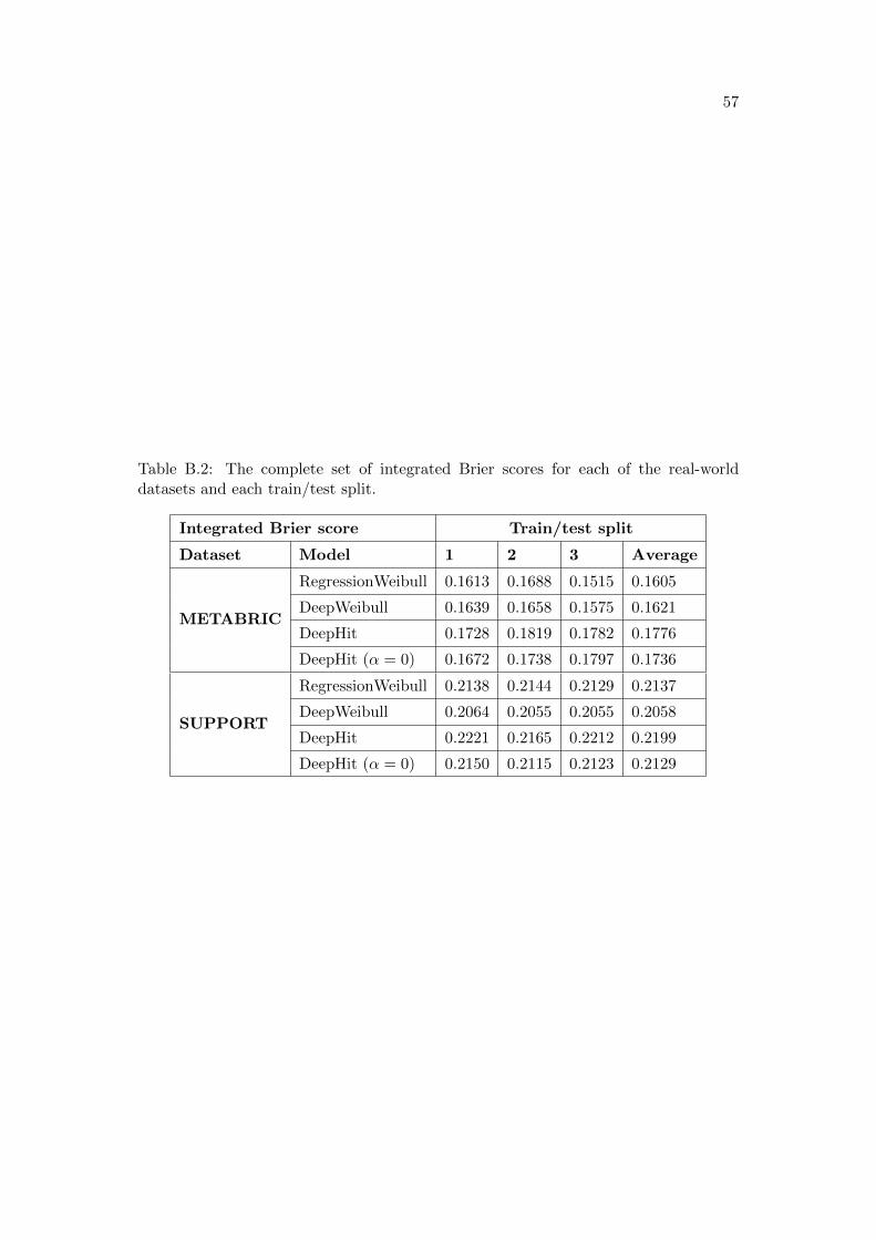
57
Table B.2: The complete set of integrated Brier scores for each of the real-worlddatasets and each train/test split.
Integrated Brier score Train/test split
Dataset Model 1 2 3 Average
METABRIC
RegressionWeibull 0.1613 0.1688 0.1515 0.1605
DeepWeibull 0.1639 0.1658 0.1575 0.1621
DeepHit 0.1728 0.1819 0.1782 0.1776
DeepHit (α = 0) 0.1672 0.1738 0.1797 0.1736
SUPPORT
RegressionWeibull 0.2138 0.2144 0.2129 0.2137
DeepWeibull 0.2064 0.2055 0.2055 0.2058
DeepHit 0.2221 0.2165 0.2212 0.2199
DeepHit (α = 0) 0.2150 0.2115 0.2123 0.2129


![A Non-parametric Bayesian Approach [WSDM’14]](https://img.pdfslide.us/doc/110x75/56816611550346895dd9594c/a-non-parametric-bayesian-approach-wsdm14.jpg)