Decompounding

ShotaGugushvili,

Frank van derMeulen, Peter

Spreij

Introduction

Non-parametricBayes

Main result

Simulations

Proof

A non-parametric Bayesian approach todecompounding from high frequency data

Shota Gugushvili Frank van der Meulen Peter Spreij

Workshop on Analysis, Geometry and Probability (and Statistics)

Ulm, October 1, 2015

Decompounding

ShotaGugushvili,

Frank van derMeulen, Peter

Spreij

Introduction

Non-parametricBayes

Main result

Simulations

Proof

Outline

1 Introduction

2 Non-parametric Bayes

3 Main result

4 Simulations

5 Proof

Decompounding

ShotaGugushvili,

Frank van derMeulen, Peter

Spreij

Introduction

Non-parametricBayes

Main result

Simulations

Proof

Compound Poisson process

N = (Nt , t ≥ 0) is a Poisson process with a constantintensity λ > 0.

Yj is a sequence of i.i.d. random variables, independentof N and having a common distribution function R withdensity r .

A compound Poisson process (CPP) X = (Xt , t ≥ 0) isdefined as

Xt =Nt∑j=1

Yj .

CPPs are basic models e.g. in risk theory and queueing.

Decompounding

ShotaGugushvili,

Frank van derMeulen, Peter

Spreij

Introduction

Non-parametricBayes

Main result

Simulations

Proof

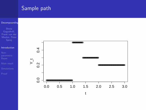
Sample path

0.0 0.5 1.0 1.5 2.0 2.5 3.0

0.0

0.2

0.4

t

Y_t

Decompounding

ShotaGugushvili,

Frank van derMeulen, Peter

Spreij

Introduction

Non-parametricBayes

Main result

Simulations

Proof

Statistical problem

The ‘true’ parameters: λ0 and r0.

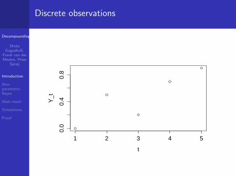
Observations: a discrete time sample X∆, . . . ,Xn∆ isavailable, where ∆ > 0 is a sampling mesh.

Problem: (non-parametric) estimation of λ0 and r0.Recovering λ0 and r0 from the observations Xi∆’s is calleddecompounding.

Some references: Buchmann and Grubel (2003),Buchmann and Grubel (2004), Comte et al. (2014),Duval (2013), van Es et al. (2007), Gugushvili etal. (2015a).

More general context of Levy processes: Comte andGenon-Catalot (2010), Comte and Genon-Catalot (2011),Neumann and Reiß (2009), and others.

Decompounding

ShotaGugushvili,

Frank van derMeulen, Peter

Spreij

Introduction

Non-parametricBayes

Main result

Simulations

Proof

Discrete observations

1 2 3 4 5

0.0

0.4

0.8

t

Y_t

Decompounding

ShotaGugushvili,

Frank van derMeulen, Peter

Spreij

Introduction

Non-parametricBayes

Main result

Simulations

Proof

Equivalent problem

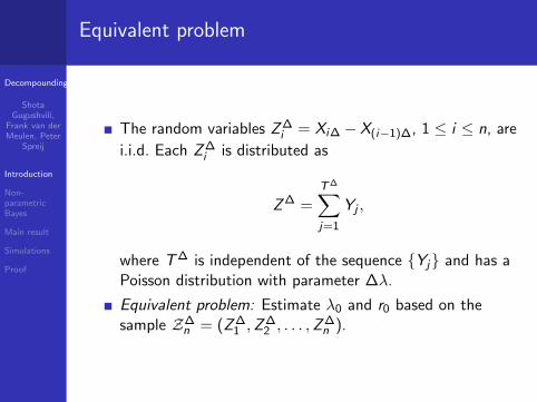
The random variables Z ∆i = Xi∆ −X(i−1)∆, 1 ≤ i ≤ n, are

i.i.d. Each Z ∆i is distributed as

Z ∆ =T∆∑j=1

Yj ,

where T ∆ is independent of the sequence Yj and has aPoisson distribution with parameter ∆λ.

Equivalent problem: Estimate λ0 and r0 based on thesample Z∆

n = (Z ∆1 ,Z

∆2 , . . . ,Z

∆n ).

Decompounding

ShotaGugushvili,

Frank van derMeulen, Peter

Spreij

Introduction

Non-parametricBayes

Main result

Simulations

Proof

Haarlemmerolie

Decompounding

ShotaGugushvili,

Frank van derMeulen, Peter

Spreij

Introduction

Non-parametricBayes

Main result

Simulations

Proof

Statistical Haarlemmerolie

Statistical Haarlemmerolie

To be or not to be?The problem seems quite tough to me!But don’t despair, my poor soul,I’ve found the way to reach the goal

By thinking hard for many daysAnd pain depicted on my face:I’ll use the rule by Thomas BayesTo elegantly close the case!

Shota Gugushvili, September 2015

Decompounding

ShotaGugushvili,

Frank van derMeulen, Peter

Spreij

Introduction

Non-parametricBayes

Main result

Simulations

Proof

Non-parametric Bayes

Non-parametric Bayesian approach to inference for Levyprocesses has been considered in the literature only inGugushvili et al. (2015a) and Gugushvili et al. (2015b).

Advantages: automatic quantification of uncertainty inparameter estimates through Bayesian posterior crediblesets; (Bayesian) adaptation.

One may also think of a non-parametric Bayes approach asa means for obtaining a frequentist estimator.

Decompounding

ShotaGugushvili,

Frank van derMeulen, Peter

Spreij

Introduction

Non-parametricBayes

Main result

Simulations

Proof

Likelihood

Bayes’ theorem combines the likelihood and prior into theposterior. We start with the likelihood.

The law Q∆λ,r of Z ∆

i is not absolutely continuous withrespect to the Lebesgue measure.

A specific choice of the dominating measure for Q∆λ,r is

not essential for inferential conclusions, but a clever choicemay greatly simplify the theoretical analysis.

Decompounding

ShotaGugushvili,

Frank van derMeulen, Peter

Spreij

Introduction

Non-parametricBayes

Main result

Simulations

Proof

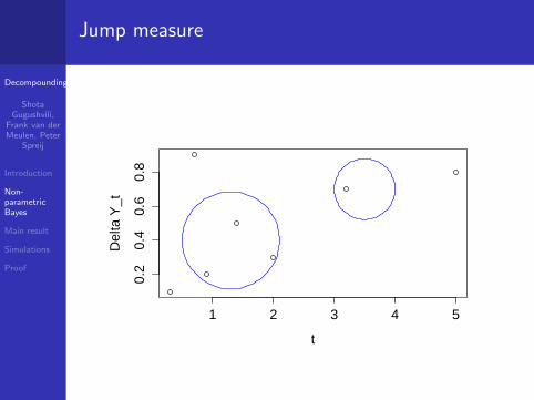
Jump measure

ForB ∈ B([0,∆])⊗ B(R \ 0)

define the random measure µ by

µX (B) = #t : (t,Xt − Xt−) ∈ B.

Let R∆λ,r be the law of (Xt : t ∈ [0,∆]).

Under R∆λ,r , the random measure µX is a Poisson point

process on [0,∆]× (R \ 0) with intensity measureΛ(dt, dx) = λdtr(x)dx .

Decompounding

ShotaGugushvili,

Frank van derMeulen, Peter

Spreij

Introduction

Non-parametricBayes

Main result

Simulations

Proof

Jump measure

1 2 3 4 5

0.2

0.4

0.6

0.8

t

Del

ta Y

_t

Decompounding

ShotaGugushvili,

Frank van derMeulen, Peter

Spreij

Introduction

Non-parametricBayes

Main result

Simulations

Proof

Continuously observed CPP

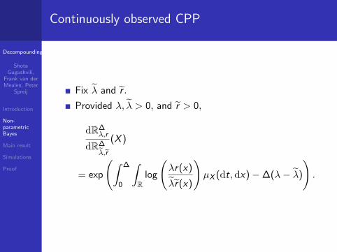
Fix λ and r .

Provided λ, λ > 0, and r > 0,

dR∆λ,r

dR∆λ,r

(X )

= exp

(∫ ∆

0

∫R

log

(λr(x)

λr(x)

)µX (dt, dx)−∆(λ− λ)

).

Decompounding

ShotaGugushvili,

Frank van derMeulen, Peter

Spreij

Introduction

Non-parametricBayes

Main result

Simulations

Proof

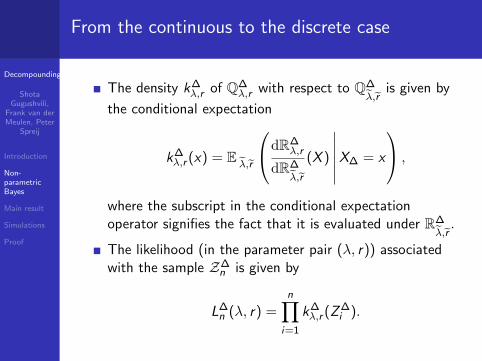
From the continuous to the discrete case

The density k∆λ,r of Q∆

λ,r with respect to Q∆λ,r

is given by

the conditional expectation

k∆λ,r (x) = E

λ,r

dR∆λ,r

dR∆λ,r

(X )

∣∣∣∣∣∣X∆ = x

,

where the subscript in the conditional expectationoperator signifies the fact that it is evaluated under R∆

λ,r.

The likelihood (in the parameter pair (λ, r)) associatedwith the sample Z∆

n is given by

L∆n (λ, r) =

n∏i=1

k∆λ,r (Z ∆

i ).

Decompounding

ShotaGugushvili,

Frank van derMeulen, Peter

Spreij

Introduction

Non-parametricBayes

Main result

Simulations

Proof

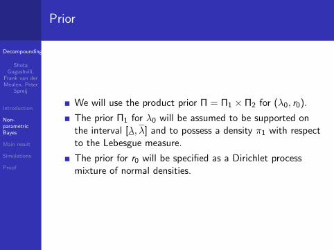
Prior

We will use the product prior Π = Π1 × Π2 for (λ0, r0).

The prior Π1 for λ0 will be assumed to be supported onthe interval [λ, λ] and to possess a density π1 with respectto the Lebesgue measure.

The prior for r0 will be specified as a Dirichlet processmixture of normal densities.

Decompounding

ShotaGugushvili,

Frank van derMeulen, Peter

Spreij

Introduction

Non-parametricBayes

Main result

Simulations

Proof

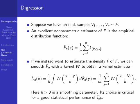
Digression

Suppose we have an i.i.d. sample V1, . . . ,Vn ∼ F .

An excellent nonparametric estimator of F is the empiricaldistribution function:

Fn(x) =1

n

n∑j=1

1[Vj≤x].

If we instead want to estimate the density f of F , we cansmooth Fn with a kernel W to obtain a kernel estimator

fnh(x) =1

h

∫W

(x − y

h

)dFn(y) =

1

nh

n∑j=1

W

(x − Vi

h

).

Here h > 0 is a smoothing parameter. Its choice is criticalfor a good statistical performance of fnh.

Decompounding

ShotaGugushvili,

Frank van derMeulen, Peter

Spreij

Introduction

Non-parametricBayes

Main result

Simulations

Proof

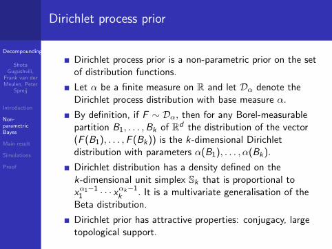
Dirichlet process prior

Dirichlet process prior is a non-parametric prior on the setof distribution functions.

Let α be a finite measure on R and let Dα denote theDirichlet process distribution with base measure α.

By definition, if F ∼ Dα, then for any Borel-measurablepartition B1, . . . ,Bk of Rd the distribution of the vector(F (B1), . . . ,F (Bk)) is the k-dimensional Dirichletdistribution with parameters α(B1), . . . , α(Bk).

Dirichlet distribution has a density defined on thek-dimensional unit simplex Sk that is proportional toxα1−1

1 · · · xαk−1k . It is a multivariate generalisation of the

Beta distribution.

Dirichlet prior has attractive properties: conjugacy, largetopological support.

Decompounding

ShotaGugushvili,

Frank van derMeulen, Peter

Spreij

Introduction

Non-parametricBayes

Main result

Simulations

Proof

Dirichlet process location mixture of normals

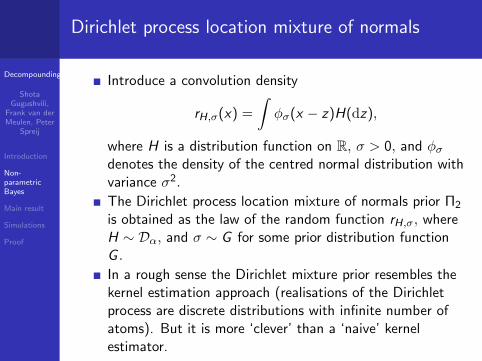
Introduce a convolution density

rH,σ(x) =

∫φσ(x − z)H(dz),

where H is a distribution function on R, σ > 0, and φσdenotes the density of the centred normal distribution withvariance σ2.

The Dirichlet process location mixture of normals prior Π2

is obtained as the law of the random function rH,σ, whereH ∼ Dα, and σ ∼ G for some prior distribution functionG .

In a rough sense the Dirichlet mixture prior resembles thekernel estimation approach (realisations of the Dirichletprocess are discrete distributions with infinite number ofatoms). But it is more ‘clever’ than a ‘naive’ kernelestimator.

Decompounding

ShotaGugushvili,

Frank van derMeulen, Peter

Spreij

Introduction

Non-parametricBayes

Main result

Simulations

Proof

Posterior

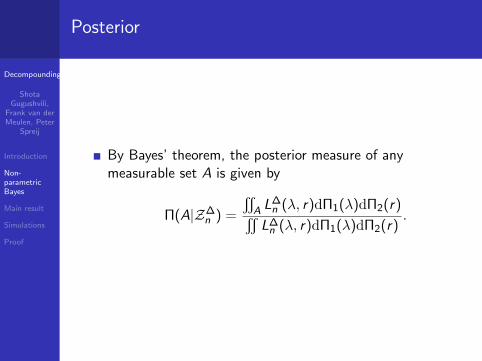
By Bayes’ theorem, the posterior measure of anymeasurable set A is given by

Π(A|Z∆n ) =

sA L∆

n (λ, r)dΠ1(λ)dΠ2(r)s

L∆n (λ, r)dΠ1(λ)dΠ2(r)

.

Decompounding

ShotaGugushvili,

Frank van derMeulen, Peter

Spreij

Introduction

Non-parametricBayes

Main result

Simulations

Proof

Asymptotic properties of Bayesian procedures

Our main result concerns study of asymptotic frequentistproperties of Bayesian procedures.

We will establish the posterior contraction rate in asuitable metric around the true parameter pair (λ0, r0).This will provide a frequentist justification of our approach.

The result also implies existence of Bayes point estimatesconverging in the frequentist sense to the true parameterpair (λ0, r0) with the same rate.

Decompounding

ShotaGugushvili,

Frank van derMeulen, Peter

Spreij

Introduction

Non-parametricBayes

Main result

Simulations

Proof

Parametric example

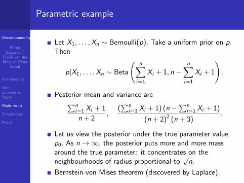
Let X1, . . . ,Xn ∼ Bernoulli(p). Take a uniform prior on p.Then

p|X1, . . . ,Xn ∼ Beta

(n∑

i=1

Xi + 1, n −n∑

i=1

Xi + 1

).

Posterior mean and variance are∑ni=1 Xi + 1

n + 2,

(∑n

i=1 Xi + 1) (n −∑n

i=1 Xi + 1)

(n + 2)2 (n + 3).

Let us view the posterior under the true parameter valuep0. As n→∞, the posterior puts more and more massaround the true parameter: it concentrates on theneighbourhoods of radius proportional to

√n.

Bernstein-von Mises theorem (discovered by Laplace).

Decompounding

ShotaGugushvili,

Frank van derMeulen, Peter

Spreij

Introduction

Non-parametricBayes

Main result

Simulations

Proof

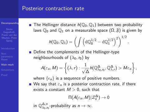
Posterior contraction rate

The Hellinger distance h(Q0,Q1) between two probabilitylaws Q0 and Q1 on a measurable space (Ω,F) is given by

h(Q0,Q1) =

(∫ (dQ1/2

0 − dQ1/21

)2)1/2

.

Define the complements of the Hellinger-typeneighbourhoods of (λ0, r0) by

A(εn,M) =

(λ, r) :

1√∆

h(Q∆λ0,r0

,Q∆λ,r ) > Mεn

,

where εn is a sequence of positive numbers.

We say that εn is a posterior contraction rate, if thereexists a constant M > 0, such that

Π(A(εn,M)|Z∆n )→ 0

in Q∆,nλ0,r0

-probability as n→∞.

Decompounding

ShotaGugushvili,

Frank van derMeulen, Peter

Spreij

Introduction

Non-parametricBayes

Main result

Simulations

Proof

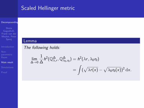
Scaled Hellinger metric

Lemma

The following holds:

lim∆→0

1

∆h2(Q∆

λ,r ,Q∆λ0,r0

) = h2(λr , λ0r0)

=

∫(√λr(x)−

√λ0r0(x))2 dx .

Decompounding

ShotaGugushvili,

Frank van derMeulen, Peter

Spreij

Introduction

Non-parametricBayes

Main result

Simulations

Proof

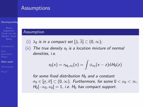
Assumptions

Assumption

(i) λ0 is in a compact set [λ, λ] ⊂ (0,∞);

(ii) The true density r0 is a location mixture of normaldensities, i.e.

r0(x) = rH0,σ0(x) =

∫φσ0(x − z)dH0(z)

for some fixed distribution H0 and a constantσ0 ∈ [σ, σ] ⊂ (0,∞). Furthermore, for some 0 < κ0 <∞,H0[−κ0, κ0] = 1, i.e. H0 has compact support.

Decompounding

ShotaGugushvili,

Frank van derMeulen, Peter

Spreij

Introduction

Non-parametricBayes

Main result

Simulations

Proof

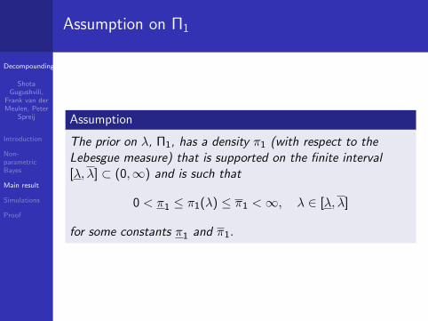
Assumption on Π1

Assumption

The prior on λ, Π1, has a density π1 (with respect to theLebesgue measure) that is supported on the finite interval[λ, λ] ⊂ (0,∞) and is such that

0 < π1 ≤ π1(λ) ≤ π1 <∞, λ ∈ [λ, λ]

for some constants π1 and π1.

Decompounding

ShotaGugushvili,

Frank van derMeulen, Peter

Spreij

Introduction

Non-parametricBayes

Main result

Simulations

Proof

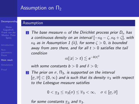
Assumption on Π2

Assumption

1 The base measure α of the Dirichlet process prior Dα hasa continuous density on an interval [−κ0 − ζ, κ0 + ζ], withκ0 as in Assumption 1 (ii), for some ζ > 0, is boundedaway from zero there, and for all t > 0 satisfies the tailcondition

α(|z | > t) . e−b|t|δ

with some constants b > 0 and δ > 0;

2 The prior on σ, Π3, is supported on the interval[σ, σ] ⊂ (0,∞) and is such that its density π3 with respectto the Lebesgue measure satisfies

0 < π3 ≤ π3(σ) ≤ π3 <∞, σ ∈ [σ, σ]

for some constants π3 and π3.

Decompounding

ShotaGugushvili,

Frank van derMeulen, Peter

Spreij

Introduction

Non-parametricBayes

Main result

Simulations

Proof

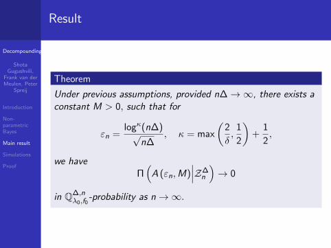
Result

Theorem

Under previous assumptions, provided n∆→∞, there exists aconstant M > 0, such that for

εn =logκ(n∆)√

n∆, κ = max

(2

δ,

1

2

)+

1

2,

we haveΠ(

A (εn,M)∣∣∣Z∆

n

)→ 0

in Q∆,nλ0,f0

-probability as n→∞.

Decompounding

ShotaGugushvili,

Frank van derMeulen, Peter

Spreij

Introduction

Non-parametricBayes

Main result

Simulations

Proof

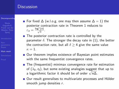
Discussion

For fixed ∆ (w.l.o.g. one may then assume ∆ = 1) theposterior contraction rate in Theorem 1 reduces toεn = logκ(n)√

n.

The posterior contraction rate is controlled by theparameter δ. The stronger the decay rate in (1), the betterthe contraction rate, but all δ ≥ 4 give the same valueκ = 1.

Our theorem implies existence of Bayesian point estimateswith the same frequentist convergence rates.

The (frequentist) minimax convergence rate for estimationof (λ0, r0), but some existing analogies suggest that up toa logarithmic factor it should be of order

√n∆.

Our result generalises to multivariate processes and Holdersmooth jump densities r .

Decompounding

ShotaGugushvili,

Frank van derMeulen, Peter

Spreij

Introduction

Non-parametricBayes

Main result

Simulations

Proof

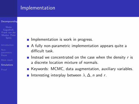
Implementation

Implementation is work in progress.

A fully non-parametric implementation appears quite adifficult task.

Instead we concentrated on the case when the density r isa discrete location mixture of normals.

Keywords: MCMC, data augmentation, auxiliary variables.

Interesting interplay between λ,∆, n and r .

Decompounding

ShotaGugushvili,

Frank van derMeulen, Peter

Spreij

Introduction

Non-parametricBayes

Main result

Simulations

Proof

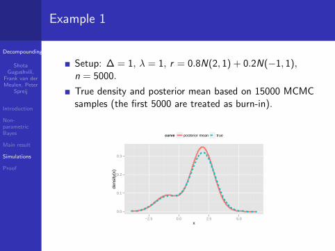
Example 1

Setup: ∆ = 1, λ = 1, r = 0.8N(2, 1) + 0.2N(−1, 1),n = 5000.

True density and posterior mean based on 15000 MCMCsamples (the first 5000 are treated as burn-in).

0.0

0.1

0.2

0.3

−2.5 0.0 2.5 5.0x

dens

ity(x

)

curve posterior mean true

Decompounding

ShotaGugushvili,

Frank van derMeulen, Peter

Spreij

Introduction

Non-parametricBayes

Main result

Simulations

Proof

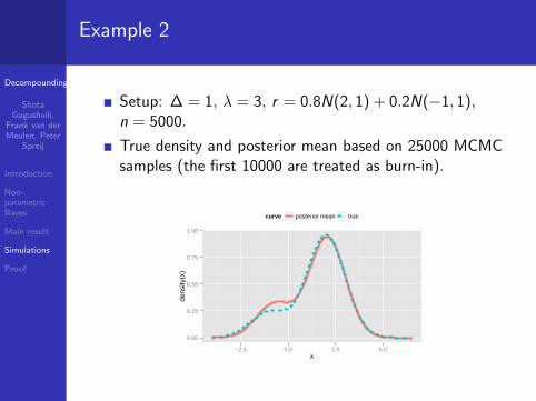
Example 2

Setup: ∆ = 1, λ = 3, r = 0.8N(2, 1) + 0.2N(−1, 1),n = 5000.

True density and posterior mean based on 25000 MCMCsamples (the first 10000 are treated as burn-in).

0.00

0.25

0.50

0.75

1.00

−2.5 0.0 2.5 5.0x

dens

ity(x

)

curve posterior mean true

Decompounding

ShotaGugushvili,

Frank van derMeulen, Peter

Spreij

Introduction

Non-parametricBayes

Main result

Simulations

Proof

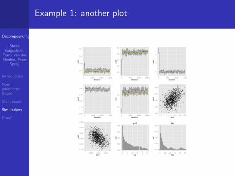
Example 1: another plot

0.2

0.3

0.4

0.5

0 5000 10000 15000iteration

psi1

0.5

0.6

0.7

0.8

0.9

0 5000 10000 15000iteration

psi2

−1

0

1

0 5000 10000 15000iteration

mu1

1.00

1.25

1.50

1.75

2.00

0 5000 10000 15000iteration

mu2

0.5

1.0

0 5000 10000 15000iteration

tau

1.85

1.90

1.95

2.00

2.05

−1.3 −1.2 −1.1 −1.0 −0.9 −0.8mu1

mu2

0.775

0.800

0.825

0.850

0.875

0.900

0.175 0.200 0.225psi1

psi2

0.00

0.25

0.50

0.75

1.00

0 10 20 30 40 50lag

acf

psi1

0.00

0.25

0.50

0.75

1.00

0 10 20 30 40 50lag

acf

tau

Decompounding

ShotaGugushvili,

Frank van derMeulen, Peter

Spreij

Introduction

Non-parametricBayes

Main result

Simulations

Proof

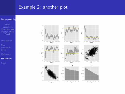
Example 2: another plot

0.4

0.8

1.2

1.6

0 5000 10000 15000 20000 25000iteration

psi1

1.6

2.0

2.4

0 5000 10000 15000 20000 25000iteration

psi2

−1

0

1

0 5000 10000 15000 20000 25000iteration

mu1

1.2

1.5

1.8

2.1

0 5000 10000 15000 20000 25000iteration

mu2

0.5

1.0

1.5

0 5000 10000 15000 20000 25000iteration

tau

1.8

2.0

2.2

−1.25 −1.00 −0.75 −0.50mu1

mu2

2.0

2.2

2.4

2.6

0.6 0.8 1.0psi1

psi2

0.00

0.25

0.50

0.75

1.00

0 10 20 30 40 50lag

acf

psi1

0.00

0.25

0.50

0.75

1.00

0 10 20 30 40 50lag

acf

tau

Decompounding

ShotaGugushvili,

Frank van derMeulen, Peter

Spreij

Introduction

Non-parametricBayes

Main result

Simulations

Proof

Roadmap

General results on posterior contraction rates (Ghosal et.al (2000), Ghosal and van der Vaart (2001) and others)are not directly applicable in our case.

However, key insights from the proofs are still valid withsuitable modifications.

Decompounding

ShotaGugushvili,

Frank van derMeulen, Peter

Spreij

Introduction

Non-parametricBayes

Main result

Simulations

Proof

Decomposition

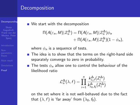
We start with the decomposition

Π(A(εn,M)|Z∆n ) = Π(A(εn,M)|Z∆

n )φn

+ Π(A(εn,M)|Z∆n )(1− φn),

where φn is a sequence of tests.

The idea is to show that the terms on the right-hand sideseparately converge to zero in probability.

The tests φn allow one to control the behaviour of thelikelihood ratio

L∆n (λ, f ) =

n∏i=1

k∆λ,f (Z ∆

i )

k∆λ0,f0

(Z ∆i )

on the set where it is not well-behaved due to the factthat (λ, f ) is ‘far away’ from (λ0, f0).

Decompounding

ShotaGugushvili,

Frank van derMeulen, Peter

Spreij

Introduction

Non-parametricBayes

Main result

Simulations

Proof

Tests

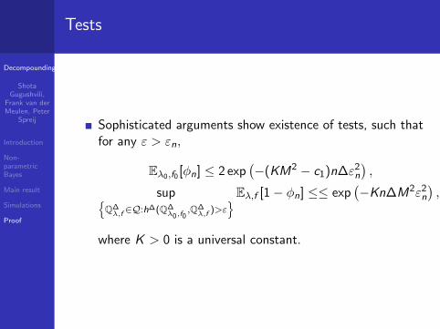
Sophisticated arguments show existence of tests, such thatfor any ε > εn,

Eλ0,f0 [φn] ≤ 2 exp(−(KM2 − c1)n∆ε2

n

),

supQ∆λ,f ∈Q:h∆(Q∆

λ0,f0,Q∆λ,f )>ε

Eλ,f [1− φn] ≤≤ exp(−Kn∆M2ε2

n

),

where K > 0 is a universal constant.

Decompounding

ShotaGugushvili,

Frank van derMeulen, Peter

Spreij

Introduction

Non-parametricBayes

Main result

Simulations

Proof

First term

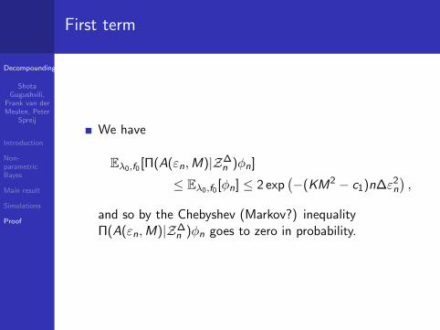
We have

Eλ0,f0 [Π(A(εn,M)|Z∆n )φn]

≤ Eλ0,f0 [φn] ≤ 2 exp(−(KM2 − c1)n∆ε2

n

),

and so by the Chebyshev (Markov?) inequalityΠ(A(εn,M)|Z∆

n )φn goes to zero in probability.

Decompounding

ShotaGugushvili,

Frank van derMeulen, Peter

Spreij

Introduction

Non-parametricBayes

Main result

Simulations

Proof

Second term

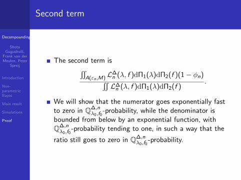
The second term iss

A(εn,M) L∆n (λ, f )dΠ1(λ)dΠ2(f )(1− φn)

sL∆n (λ, f )dΠ1(λ)dΠ2(f )

.

We will show that the numerator goes exponentially fastto zero in Q∆,n

λ0,f0-probability, while the denominator is

bounded from below by an exponential function, withQ∆,nλ0,f0

-probability tending to one, in such a way that the

ratio still goes to zero in Q∆,nλ0,f0

-probability.

Decompounding

ShotaGugushvili,

Frank van derMeulen, Peter

Spreij

Introduction

Non-parametricBayes

Main result

Simulations

Proof

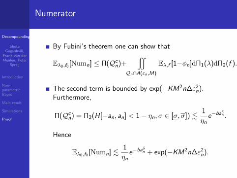
Numerator

By Fubini’s theorem one can show that

Eλ0,f0 [Numn] ≤ Π(Qcn)+

x

Qn∩A(εn,M)

Eλ,f [1−φn]dΠ1(λ)dΠ2(f ).

The second term is bounded by exp(−KM2n∆ε2n).

Furthermore,

Π(Qcn) = Π2(H[−an, an] < 1− ηn, σ ∈ [σ, σ]) .

1

ηne−ba

δn .

Hence

Eλ0,f0 [Numn] .1

ηne−ba

δn + exp(−KM2n∆ε2

n).

Decompounding

ShotaGugushvili,

Frank van derMeulen, Peter

Spreij

Introduction

Non-parametricBayes

Main result

Simulations

Proof

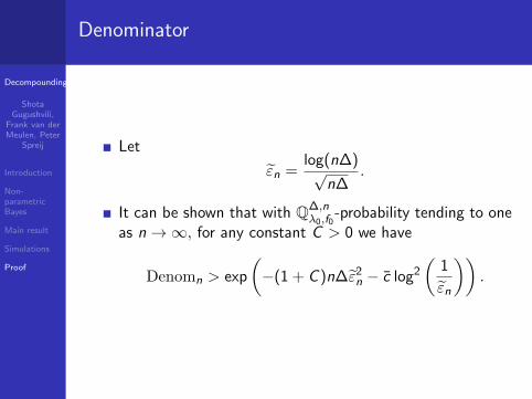
Denominator

Let

εn =log(n∆)√

n∆.

It can be shown that with Q∆,nλ0,f0

-probability tending to oneas n→∞, for any constant C > 0 we have

Denomn > exp

(−(1 + C )n∆ε2

n − c log2

(1

εn

)).

Decompounding

ShotaGugushvili,

Frank van derMeulen, Peter

Spreij

Introduction

Non-parametricBayes

Main result

Simulations

Proof

Completion of the proof

The proof is completed by combining the previous bounds:provided the constant M > 0 is chosen large enough, theChebyshev inequality yields the result.