1

Deep Dictionary Learning: A PARametricNETwork Approach

Shahin Mahdizadehaghdam, Member, IEEE, Ashkan Panahi, Member, IEEE, Hamid Krim, Fellow, IEEE,Liyi Dai, Fellow, IEEE

Abstract— Deep dictionary learning seeks multiple dictionaries at different image scales to capture complementary coherentcharacteristics. We propose a method for learning a hierarchy of synthesis dictionaries with an image classification goal. Thedictionaries and classification parameters are trained by a classification objective, and the sparse features are extracted by reducing areconstruction loss in each layer. The reconstruction objectives in some sense regularize the classification problem and inject sourcesignal information in the extracted features. The performance of the proposed hierarchical method increases by adding more layers,which consequently makes this model easier to tune and adapt. The proposed algorithm furthermore, shows remarkably lower foolingrate in presence of adversarial perturbation. The validation of the proposed approach is based on its classification performance usingfour benchmark datasets and is compared to a CNN of similar size.

Index Terms—Image classification, deep learning, sparse representation.

F

1 INTRODUCTION

T HE key step to the complex task of classifying images isthat of obtaining features of these images which encompass

relevant information, e.g., label information. The two most well-known research directions in this regard are Deep Neural Networksand Dictionary Learning for Sparse Representation.

Deep Neural Networks: In recent years, Deep Neural Networks(DNNs), and more specifically Convolutional Neural Networks(CNNs) [5], [20], showed impressive results in many applications,in particular, signal and image processing [6], [35]. A Convolu-tional Neural Network consists of multiple layers and a differentnumber of filters in each layer. Despite these significant achieve-ments, there is still little theoretical understanding of the learningprocess in these networks. Invariant scattering convolution [4] isamong the few works to provide a theoretical perspective of CNN.This technique specializes the filters in CNN to be fixed waveletfunctions. As the wavelet transform is invariant to translation androtation, the features from the scattering transform are invariant tothese transformations as well.

Dictionary Learning for Sparse Representation: Parsimoniousdata representation by learning overcomplete dictionaries hasshown promising results in a variety of problems such as imagedenoising [7], image restoration [39], audio processing [11], andimage classification [41]. This frame-like representation of eachdata vector as a linear combination of atoms carries a sparse notionof the associated coefficients. Using Sparse Representation-basedClassification (SRC) [37], one can represent an image as a com-bination of a few images in the training dataset. This is followedsubsequently by a classifier based on these feature vectors. Theproposed refinements were task-driven dictionary learning [22]and Label Consistent K-SVD (LC-KSVD) [17] which jointly learn

• S. Mahdizadehaghdam, A. Panahi, and H. Krim are with the Departmentof Electrical and Computer Engineering, North Carolina State University,Raleigh, NC 27695 USA.E-mail: smahdiz@ncsu.edu; apanahi@ncsu.edu; ahk@ncsu.edu

• L. Dai is with Army Research Office, RTP, Raleigh, NC 27703 USA.E-mail: liyi.dai.civ@mail.mil

an overcomplete dictionary, sparse representation, and classifica-tion parameters.

The aforementioned dictionary learning methods are based onentire images for training the dictionary and finding the sparserepresentation, which can be computationally expensive. Thesepotentially lead to a poor performance when the training dataset issmall. Convolutional Neural Networks, however, learn the initialfeatures from small image patches and build a hierarchy of thefeatures at different scales. Contrary to conventional wisdom,several experimental studies [12], [13] have reported that deeperneural networks are more difficult to train, and adding morelayers, eventually leads to decreased performance. Part of thethis mentioned problem is due to the vanishing/exploding gradienteffect during training. This problem persists despite mitigationssuch as batch normalization [13].

To cope with the CNN’s fore-noted limitations, and to exploitthe deep structure intrinsic to data, we propose a principledhierarchical (deep) dictionary learning to be learned while achiev-ing optimal classification. Within this framework, the front layerdictionary is learned on small image patches, and the subsequentlayer dictionaries are learned on larger scales. Put simply, theinitial scale captures the fine low-level structures comprising theimage vectors, while the next scales coherently capture morecomplex structures. The classification is ultimately carried outby assembling the final and largest scale features of an imageand assessing their contribution. In contrast to CNN, we showthat the performance of the proposed DDL method improves withadditional layers, hence indicating an amenability to tuning, and abetter potential for more elaborate learning tasks such as transferlearning.

Inspired by the study in [31] on neural networks, we show,using an information theoretic argument that DDL is a sensibleapproach to image classification. We show that under a cer-tain generative model, DDL maximizes the mutual informationI(A∗,Y ) between the optimal representation of the observeddata/signals and the labels. The optimal representation, A∗, isobtained by maximizing their mutual information I(X,A) with

arX

iv:1

803.

0402

2v1

[cs

.CV

] 1

1 M

ar 2

018

2

the input signals. In the dictionary learning framework, we showthat the proposed model simplifies to a joint learning of thedictionary and the classification parameter, which we subsequentlygeneralize into hierarchically/deeply learning the dictionaries overdifferent layers.

On account of the parsimony of our dictionary atom repre-sentation of features at each layer, our proposed method exhibitsa remarkably lower fooling rate to adversarial perturbation andrandom noises. In light of the limited performance of the state ofthe art classifiers as a result of a single additive perturbation [9],[27], [28], the robustness displayed by our proposed algorithmis significant and points to a promise of the approach. Ourcontributions in this paper are summarized as as follows:• One of the novelties of this paper is in rigorously showing the

importance of aiming for a high mutual information betweenthe original signal and the output of each layer. This is in factin agreement with the conclusion of the Residual Network [13],where a direct connection of increasing the number of layers inCNN with the drop in performance has been made. Our paperestablishes that preserving a high fidelity to the input signal (byway of a layer-based LASSO-regularization) is the key to havingdeeper models with no performance loss in classification.

• The proposed algorithm is robust to adversarial perturbation andrandom noises.

• A theoretical discussion on the model-hyperparameter selectionis provided. We established a relation between the secondmoment of the input signal and the necessary width of eachlayer.

The balance of the paper is organized as follows: In Section2, we provide the problem statement as well as some backgroundinformation of relevance to this paper. We formulate and proposeour new approach in Section 3. The neural networks and theproposed method are compared from an information theoreticpoint of view in Section 4. The theoretical discussion about thehyper-parameter selection is in Section 5. Substantiating exper-imental results are presented in Section 6. Finally, we providesome concluding remarks in Section 7.

2 PROBLEM STATEMENT AND PRELIMINARIES

Image classification is typically based on learning a synthesisdictionary which yields representations of each image as a sparselinear combination of the atoms of the learned dictionary [23].This is typically followed by a classification technique, such asSVM [15], a neural network, or a linear classifier operating on thesparse feature vectors. With that goal in mind, one can vectorizeall training images into a matrix and perform dictionary learningand sparse representation [24].

Given vectorized images, gi ∈ Rm i ∈ {1, .., n}, as a matrixG, the optimal dictionary D∗ ∈ Rm×k and the optimal sparserepresentations of the images, a∗i ∈ Rk (the columns of the matrixA∗), can be be learned by minimizing the reconstruction lossfunction LR(D,A,G):

{A∗,D∗} = arg minA, D

LR(D,A,G),

LR(D,A,G) =1

2||G−DA||2F + λ||A||1 + λ′||A||2F ,

A ≥ 0, and D ∈ C,(1)

where C is the convex set of matrices with unit L2-norm columns.The regularizers of Eqn. (1) are for a sample setting and may

vary with the problem at hand. Different types of regularizationmay be imposed on the feature vectors for specific task. Havingthe optimal representation A∗, and the label information of theimages Y , the desired classifier can be trained by minimizing theclassification loss function LC(Y ,A∗,W ) over the classificationparameter W :

W ∗ = arg minW

LC(Y ,A∗,W ). (2)

Although the formulation in Eqn. (1) can achieve a very lowerror in reconstruction of the original image from the extractedsparse features, these feature vectors are not necessarily optimalfor classification purposes. More generally, studies in recent yearshave shown that isolating the dictionary learning from classifica-tion yields suboptimal dictionaries for classification purposes [1],[21]. Thus, more advanced methods have been proposed to jointlytrain the dictionary and the classification models. These methods,in general, attempt to learn a dictionary for the purpose ofclassification. Among these, figure supervised dictionary learningmethods [26]. Aside from the subtle differences among the lattermethods, they are commonly based on jointly learning classifi-cation parameters, a dictionary and sparse representations from aloss function, which is usually a summation of a reconstructionloss (similar to LR in Eqn. (1)) and a classification loss:

{W ∗,D∗,A∗} = arg minW ,D,A

LR(D,A,G) + LC(Y ,A,W ).

(3)Task-driven dictionary learning methods [22], on the other hand,seek the optimum dictionary and classification parameters by min-imizing a loss function which is based on only the classificationloss. The feature vectors in these cases are, however, conditionedto form optimal sparse representation:

{W ∗,D∗} = arg minW ,D

LC(Y ,A∗,W ),

s.t. : A∗ = arg minA

LR(D,A,G).(4)

Despite the similarities to formulation Eqns. (2) & (3), the latterone is relatively more general, achieves a higher performance forlarge image datasets and is easier to train by a gradient decentapproach [22].

Our work here, is in line with the task-driven dictionarylearning methods with an additional set of deep dictionaries tocapture structure at different scales [21].

3 PROPOSED SOLUTION

Our approach to classifying images starts by learning a classi-fication model with input features/coefficients obtained from thelast layer of a sequential hierarchy of dictionaries. Specifically,for an s-layer hierarchy, the classification parameters, and thedictionaries are learned by minimizing the following classificationloss functional:

{W ∗, {D∗(r)}sr=1} = arg minW , {D(r)}sr=1

LC(Y ,X∗(s),W ),

(5)where W , D(r), and Y are respectively the classification pa-rameters, the dictionary for layer r, and the labels of the trainingimages. X∗(s) is the input to the classifier which is calculatedby concatenating the output vectors A∗(s) of the last layer asshortly explained. More generally, X∗(r) denotes the input to the

3

Images

𝑿𝑿(0)

… … … … …

… … …

…

…

… … … …

… … … …

… … … …

… … … … …

Layer 1

𝑫𝑫(1)𝑿𝑿∗(1)

= 𝑃𝑃1(𝑨𝑨∗(1))

Layer 𝑠𝑠

𝑫𝑫(2)

… … … … …

… … …

…

…

… … … …

… … … …

… … … …

𝑿𝑿∗(𝑠𝑠−1)

= 𝑃𝑃𝑠𝑠−1(𝑨𝑨∗(𝑠𝑠−1))

𝑨𝑨∗(𝑠𝑠)

𝑫𝑫(𝑠𝑠)

… … … … …

Layer 2

…

Classifier𝑿𝑿∗(𝑠𝑠) = 𝑃𝑃𝑠𝑠(𝑨𝑨∗(𝑠𝑠))

𝑾𝑾

…

𝑠𝑠21

𝑨𝑨∗(2)𝑨𝑨∗(1)

= arg min𝑨𝑨 1

ℒ1ℛ(𝑫𝑫 1 ,𝑨𝑨 1 ,𝑿𝑿∗(0)) = arg min𝑨𝑨 2

ℒ2ℛ(𝑫𝑫 2 ,𝑨𝑨 2 ,𝑿𝑿∗(1)) = arg min𝑨𝑨 𝑠𝑠

ℒ𝑠𝑠ℛ(𝑫𝑫 𝑠𝑠 ,𝑨𝑨 𝑠𝑠 ,𝑿𝑿∗(𝑠𝑠−1))

ℒ𝒞𝒞(𝒀𝒀,𝑿𝑿∗ 𝑠𝑠 ,𝑾𝑾)

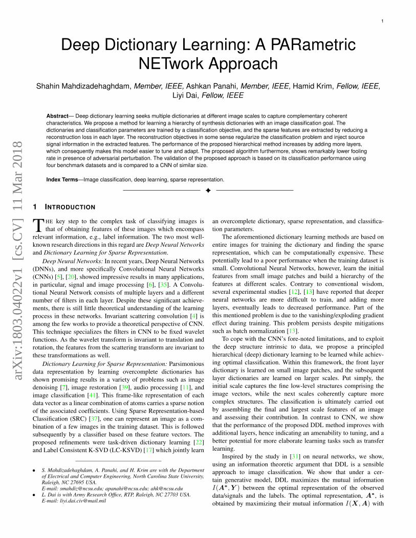
Fig. 1: Sequential steps of a deep dictionary with s layers.

(r + 1)th layer while A∗(r) refers to the output of the rth layer.These vectors are the result of the following recursive relation:

A∗(r) = arg minA(r)

LRr (D(r),A(r),X∗(r−1)),

s.t. :

LRr (D(r),A(r),X∗(r−1)) =1

2||X∗(r−1) −D(r)A(r)||2F

+ λ||A(r)||1,+λ′||A(r)||2F ,X∗(r) = Pr(A

∗(r)),

D(r) ∈ C, A(r) ≥ 0,(6)

where each column of the matrix X∗(0) is a vectorized imagepatch, and Pr is an operator which concatenates the feature vectorsof adjacent patches from the previous layer. In other words, Pr isan operator which reshapes the output of layer r as the input tolayer (r + 1). Eqn. (6) is similar to an elastic net regularizationproblem with a non-negativity condition on the feature vectors.We emphasize that the objective functional in Eqn. (5) implicitlydepends on all dictionaries, since the computation of X∗(s) inEqn. (6) requires them.

We show in Fig. 1 the sequence of computational stepsexploiting matrices from Eqn. (6) and their associated structures.The white arrows in the figure depict the forward computing pathof the sparse representation of each input layer. A set of imagesare first segmented into small image patches and vectorized intomatrix X(0) as the input of the first layer. For a given first layerdictionary D(1), the sparse representations of the image patchesare learned as the columns of the A∗(1) matrix, by solving Eqn.(6) via the sparse encoding algorithm FISTA [2]. The patches ofA∗(1) (3 × 3 window) are next reshaped by operator P1 to yieldinput X∗(1) to the second layer. This analysis is sequentiallycarried on to scale s where A∗(s) yields X∗(s) as an input toa classifier (such that each column of this matrix represents animage). The class label information of the images in matrix Y ,together with X∗(s) provide the classification parameters W as asolution to Eqn. (5).

The blue arrows in Fig. 1 highlight the backward trainingpath, reflecting the updates on the dictionaries as a result of theoptimized classification, by way of gradient descent on Eqn. (5).Optimizing the classification loss LC in the forward pass (path ofFig. 1), is followed by updates on the backward pass (path of Fig.1).

In summary, the relevant parameter vectors of the images

are learned through multiple forward-backward passes throughthe layers. The dictionaries are updated such that the resultingrepresentations are suitable for the classification. Moreover, therepresentations are learned by minimizing the reconstruction lossat each layer. The search for the optimal classifier is not onlycarried out by accounting for the deep structure of images, it isadditionally regularized by preserving the fidelity of image contentrepresentation. We further discuss the derivation rationale of ourpurposed approach in Section 4.

3.1 AlgorithmAlgorithm 1, discusses the details of the updating procedure of theparameters in our method.

Lines 1-4: We randomly initialize the dictionaries and theclassification parameter.

Lines 6-12: During the training phase, we randomly select asubset of images, and we construct the representation of the im-ages by sequentially solving the problem in (line 9) and preparingthe input for the next layer in (line 10). Our solution to the problemin (line 9) is obtained via the sparse coding algorithm FISTA [2].In (line 12), we calculate the classification loss for the selectedsubset of the images.

Lines 13-15: The classification parameter and the dictionariesare updated via the gradient of the computed loss in (lines 13 and15), respectively. η is the step size.

3.2 Optimization by Gradient DescentDepending on the choice of the classification functional, comput-ing the gradient of the loss functional with respect to the classi-fication parameter, ∂L

C

∂W , can conceptually be straightforward. Toensure an updating step of the stochastic gradient descent for thedictionary at layer r, we require ∂LC

∂D(r) .Claim: The matrix form of ∂LC

∂D(r) is given by,

∂LC

∂D(r)= −D(r)β(r)a∗(r)T + (x∗(r−1) −D(r)a∗(r))β(r)T ,

β(r)Λ = (D

(r)TΛ D

(r)Λ + λ′I)−1 · ∂LC

∂a∗(r)Λ

,

β(r)

ΛC= 0,

(7)where Λ is the active set of a∗, Λ , {j | a∗[j] 6= 0, j ∈{1, .., k}}, ΛC is the complement of set Λ, I is an identity matrix,1 is a one-vector, and x∗(r) is an arbitrary column of X∗(r).

4

Algorithm 1Initialization:

1: for r in {1, s} do:2: Initialize D(r)

0 randomly.3: end for4: Initialize W 0 randomly.

Training:5: for t in {1, T} do:

Forward pass:6: Randomly select a set of images from the training dataset.7: Patch and vectorize the images as the columns of X(0)

t .8: for r in {1, s} do:9: A

∗(r)t = argmin

A(r)tLRr (D

(r)t ,A

(r)t ,X

∗(r−1)t ).

10: X∗(r)t = Pr(A

∗(r)t ).

11: end for12: LC

t = LC(Y t,X∗(s)t ,W t).

Backward pass:13: W t+1 = W t − η ∂L

Ct

∂W t.

14: for r in {1, s} do:15: D

(r)t+1 = D

(r)t − η

∂LCt∂D

(r)t

.16: end for17: end for

The aforementioned gradient derivation is built on the work in[22] for a deep network. The steps of deriving this gradient by thechain rule is as follows,

∂LC

∂D(r)= (

∂LC

∂x∗(r))T · [∂x

∗(r)1

∂D(r), ..,

∂x∗(r)m

∂D(r)],

∂x∗(r)

∂D(r)= Pr(

∂A∗(r)

∂D(r)),

(8)

where x∗(r) is an arbitrary column of X∗(r), and A∗(r)

arethe corresponding output feature vectors from layer r such thatPr(A

∗(r)) = x∗(r). In addition, x∗(r)i , is the ith element of the

vector x∗(r). The term ∂A∗(r)

∂D(r) , is the gradient of a matrix with

respect to a matrix, it is organized as a tensor with rank 4. ∂x∗(r)

∂D(r)

is also a tensor of rank 3. Because x∗(r) is obtained as a resultof a reshaping operator on A

∗(r), the same reshaping operator

can be applied to compute the gradient. The term ∂LC∂x∗(r)

can becomputed by applying the chain rule.

In order to compute ∂A∗(r)

∂D(r) , we temporarily drop the su-perscripts for simplicity. Consider dj as the jth column of theD(r) matrix, x as a column of X∗(r−1) matrix, and a as thecorresponding feature vector. The vector a∗ is an optimal solutionof Eqn. (6) if and only if,

(DTΛDΛ + λ′I)a∗Λ = DT

Λx− λ1, (9)

We carry out element-wise computation of ∂a∗

∂D , by taking thegradient of both sides of Eqn. (9) with respect to the elements ofthe D matrix:

∂a∗Λ∂d(i,j)

= (DTΛDΛ +λ′I)−1(

∂DTΛx

∂d(i,j)− ∂D

TΛDΛ

∂d(i,j)a∗Λ). (10)

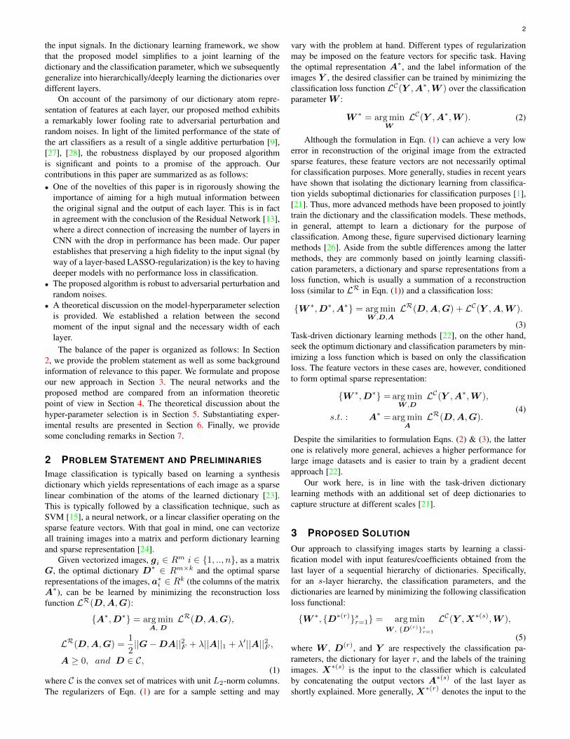
Feature Extraction/ Coder Classifier

A model with parameter 𝜽𝜽

𝑿𝑿 𝑨𝑨 �𝒀𝒀

Fig. 2: X and A are respectively, the images and the associatedfeature vectors. Y represents the class labels, and Y is theestimated class labels by the classifier.

Further simplifying the equation above and restoring the su-perscripts, we can write the ∂LC

∂D(r) in matrix format as follows,

∂LC

∂D(r)= −D(r)β(r)a∗(r)T + (x∗(r−1) −D(r)a∗(r))β(r)T ,

β(r)Λ = (D

(r)TΛ D

(r)Λ + λ′I)−1 · ∂LC

∂a∗(r)Λ

,

β(r)

ΛC= 0.

(11)

4 AN INFORMATION THEORETIC PERSPECTIVE OFDEEP LEARNING

The goal of this section is to compare neural network withdictionary learning by the proposed method in an information-theoretic framework.

Consider a setting with X = [x1, ..,xn] as the original inputsignals and Y = [y1, ..,yn] as the true label information of theoriginal signals (Fig. 2). Starting with the original input signals,the favorable classification model, in this case, is expected to yieldthe feature vectors A = [a1, ..,an], whose mutual informationwith the labels Y = [y1, ..,yn] is maximal. In addition toseeking the maximum mutual information with the labels, ourmethod additionally seeks to attain maximum mutual informationbetween the feature vectors and the original signals. To this end,and from an information theoretic point of view, we characterizeour classifier as follows,

θ∗ = arg maxθ

I(A∗(s),Y ), (P1)

st : A∗(r) = arg maxA(r)

I(X∗(r−1),A(r)), r ∈ {1, .., s}(12)

where I(X,A) is the mutual information between X and A,and θ is the model parameter. The optimization problem in Eqn.(12) seeks θ, by maximizing the mutual information between thelabels and the optimal feature vectors, A∗, which by virtue ofthe constraint, have maximal mutual information with the originalsignal.Proposition: Considering the following generative model, weshow that the favorable classification model in (P1) is approxi-mately equal to a single-layer DL followed by classification by theproposed method:

• The generated signals {xi} are independent and follow aGaussian distribution p(xi|ai) ∝ e−||xi−Dai||22 .

• The features {ai} are non-negative latent variables with aprior as a compromise between the Gaussian and Laplacepriors: p(ai) ∝ e−λ||ai||1−λ

′||ai||22 .

5

1 2 3 4 5 6 7 8 90

1

2

3

4

5

6

7

DDLALL-CNN

(a) Epoch 1, Iteration 1

1 2 3 4 5 6 7 8 90

1

2

3

4

5

6

7

DDLALL-CNN

(b) Epoch 1, Iteration 10

1 2 3 4 5 6 7 8 90

1

2

3

4

5

6

7

DDLALL-CNN

(c) Epoch 25, Iteration 1865

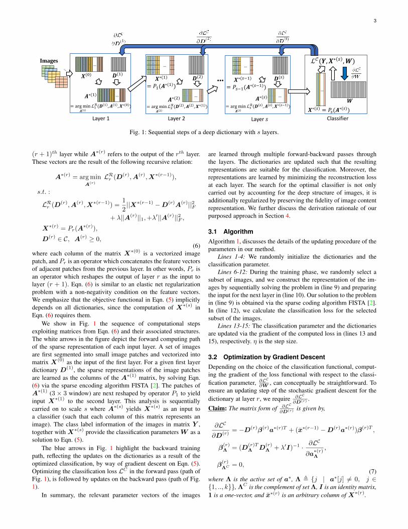
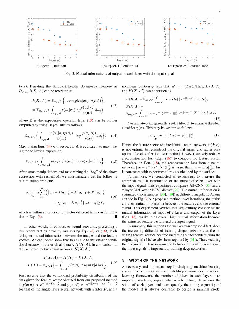
Fig. 3: Mutual informations of output of each layer with the input signal

Proof. Denoting the Kullback-Leibler divergence measure asDKL, I(X,A) can be rewritten as,

I(X,A) = Exi∈X

{DKL(p(ai|xi)||p(ai))

},

= Exi∈X

{∫ai∈A

p(ai|xi)logp(ai|xi)p(ai)

dai},

(13)

where E is the expectation operator. Eqn. (13) can be furthersimplified by using Bayes’ rule as follows,

Exi∈X

{∫ai∈A

p(xi|ai)p(ai)p(xi)

logp(xi|ai)p(xi)

dai}. (14)

Maximizing Eqn. (14) with respect toA is equivalent to maximiz-ing the following expression,

Exi∈X

{∫ai∈A

p(xi|ai)p(ai) log p(xi|ai)dai}. (15)

After some manipulations and maximizing the “log” of the aboveexpression with respect A, we approximately get the followingminimization problem:

arg min{ai}

n∑i=1

(||xi −Dai||22 + λ||ai||1 + λ′||ai||22

+log||xi −Dai||22), st : ai ≥ 0,

(16)

which is within an order of log factor different from our formula-tion in Eqn. (6).

In other words, in contrast to neural networks, preserving alow reconstruction error by minimizing Eqn. (6) or (16), leadsto higher mutual information between the images and the featurevectors. We can indeed show that this is due to the smaller condi-tional entropy of the original signals, H(X|A), in comparison tothat achieved by the neural network, H(X|A′):

I(X,A) = H(X)−H(X|A),

= H(X)− Ea∈A

{−∫x∈X

p(x|a) log p(x|a)dx}.

(17)

First assume that the conditional probability distribution of thedata given the feature vector obtained from our proposed methodis p(x|a) ∝ e−||x−Da||22 and p(x|a′) ∝ e−||x−ϕ

−1(F−1a′)||22

for that of the single-layer neural network with a filter F , and a

nonlinear function ϕ such that, a′ = ϕ(Fx). Thus, H(X|A)and H(X|A′) can be written as,

H(X|A) = Ea∈A{∫

x∈X||x−Da||22 e−||x−Da||22 dx

},

H(X|A′) =

Ea∈A′

{∫x∈X

||x− ϕ−1(F−1a′)||22 e−||x−ϕ−1(F−1a′)||22 dx}.

(18)Neural networks, generally, seek a filter F to estimate the ideal

classifier γ(x). This may be written as follows,

arg minF

||ϕ(Fx)− γ(x)||22. (19)

Hence, the feature vector obtained from a neural network, ϕ(Fx),is not optimal to reconstruct the original signal and rather onlyoptimal for classification. Our method, however, actively reducesa reconstruction loss (Eqn. (16)) to compute the feature vector.Therefore, in Eqn. (18), the reconstruction loss from a neuralnetwork, ||x− ϕ−1(F−1a′)||22, is larger than ||x−Da||22. Thisis consistent with experimental results obtained by the authors.

Furthermore, we conducted an experiment to measure theempirical mutual information of the output of each layer withthe input signal. This experiment compares All-CNN [33] and a9-layer DDL over MNIST dataset [20]. The mutual information isestimated (from samples [30], [19]) at different snapshots. As onecan see in Fig. 3, our proposed method, over iterations, maintainsa higher mutual information between the features and the originalsignal. This experiment verifies that sequentially conserving themutual information of input of a layer and output of the layer(Eqn. 12), results in an overall high mutual information betweenthe extracted feature vectors and the input signal.

In summary, this supports the well-known empirical fact aboutthe increasing difficulty of training deeper networks, as the re-sulting feature vectors become increasingly independent from theoriginal signal (this has also been reported by [31]). Thus, securingthe maximum mutual information between the feature vectors andthe input signals is important to training deep networks.

5 WIDTH OF THE NETWORK

A necessary and important step in designing machine learningalgorithms is to set/tune the model-hyperparameters. In a deeplearning framework, the number of filters in each layer is animportant model-hyperparameter which in turn, determines thewidth of each layer, and consequently the fitting capability ofthe model. It is always desirable to design a minimal model

6

with a sufficient number of parameters in each layer to learnthe true structure of the data. In most computer vision problems,the real structure of the data is generally unknown, and pickingthe number of parameters in each layer is not straightforward.An experimentally-proven rule for designing CNN is that, widelayers are good at memorization of the output value for a trainingdataset, but not so good at generalization in the inference phase.While the selection of model-hyperparameters for CNN remainslargely heuristic, e.g., random selection search [3], or visualizationtechniques [40], we provide in this section, some principle inselecting the width of layers in the proposed DDL. Specifically,we propose a rationale for a wider first layer (with a larger numberof dictionary atoms) relative to the subsequent layers.

We show that the second moment of the input signal to eachlayer is an important factor for selecting the number of dictionaryatoms in that layer. More specifically, we show that input signalswith higher second moments require a larger number of dictionaryatoms to keep the reconstruction error small. This consequently,secures a maximal mutual information between the input signalto the layer and the resulting sparse representations. Consider aleast-squares optimization problem as follows,

mina

1

2||x−Da||22 + λ||a||1, (20)

where x is assumed to consist of independent and centered Gaus-sian entries, with equal variances σ2, and the matrix D ∈ Rm×nis a known dictionary. Then, it is desired to characterize thestatistical behavior of the optimal solution a of Eqn. (20), alsocalled the estimate.

Theorem 1. Considering the least-square optimization problemof Eqn. (20), the asymptotic value of E(a2) is characterized asfollows,

E[a2] = 2(p2 +λ2p2

β2)Q(

λ

β)− 2λp2

β√

2πexp(− λ2

2β2), (21)

where the function Q(.) is the Gaussian tail Q-function, p and βare the solutions of the following two-dimensional optimization,

maxβ≥0

minp>0{pβ(γ − 1)

2+γσ2β

2p− γβ2

p+ pF (β)}, (22)

F (q) =λe− λ2

2q2

2√

2π− q

2(1 +

λ2

q2)Q(

λ

q) +

q

4, (23)

and γ = m/n determines the ratio of the number of rows to thenumber of columns (atoms) of the dictionary.

Proof. See Appendix A.

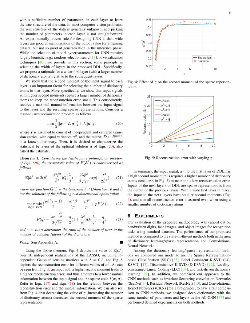
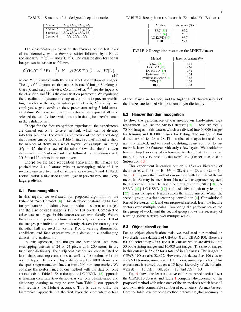
Using the above theorem, Fig. 4 depicts the value of E[a2]over 50 independent realizations of the LASSO, including in-dependent Gaussian sensing matrices with λ = 0.5, and Fig. 5depicts the reconstruction error for different values of σ2. As canbe seen from Fig. 5, an input with a higher second moment leads toa higher reconstruction error, and thus amounts to a lower mutualinformation between the input signal and the sparse code I(x,a).Refer to Eqn. (17) and Eqn. (18) for the relation between thereconstruction error and the mutual information. We can also seefrom Fig. 4, that decreasing the value of γ (increasing the numberof dictionary atoms) decreases the second moment of the sparserepresentation.

0 2 4 6 8 100.15

0.2

0.25

0.3

0.35

0.4

0.45

TheoreticalEmpirical

Fig. 4: Effect of γ on the second moment of the sparse repersen-tation.

0 2 4 6 8 10.

0

5

10

15

20

25

Rec

onst

ruct

ion

Err

or

<2=0.5

<2=1.5

<2=2.5

<2=3.5

<2=4.5

Fig. 5: Reconstruction error with varying γ.

In summary, the input signal, x0, to the first layer of DDL hasa high second moment thus requires a higher number of dictionaryatoms (smaller γ in Fig. 5) to maintain a low reconstruction error.Inputs of the next layers of DDL are sparse representations fromthe output of the previous layers. With a wide first layer in place,the input to the next layers have smaller second moments (Fig.4), and a small reconstruction error is assured even when using asmaller number of dictionary atoms.

6 EXPERIMENTS

Our evaluation of the proposed methodology was carried out onhandwritten digits, face images, and object images for recognitiontasks using standard datasets. The performance of our proposedmethod is compared to the state-of-the-art methods both in the areaof dictionary learning/sparse representation and ConvolutionalNeural Networks.

Among the dictionary learning/sparse representation meth-ods we compared our model to are the Sparse Representation-based Classification (SRC) [38], Label Consistent K-SVD (LC-KSVD) [17], Discriminative K-SVD (D-KSVD) [42], Locality-constrained Linear Coding (LLC) [36], and task-driven dictionarylearning [22]. In addition, we compared our approach to theCNN methods such as invariant Scattering convolution Networks(ScatNet) [4], Residual Network (ResNet) [13], and ConvolutionalKernel Networks (CKN) [25]. Furthermore, to have a fair compar-ison to CNN methods, we designed deep dictionaries with thesame number of parameters and layers as the All-CNN [33] andperformed detailed experiments on both methods.

7

TABLE 1: Structure of the designed deep dictionaries

Section 1 M1, 2M1, 4M1,M1

Section 2 M2, 2M2, 4M2,M2

Section 3 M3, 2M3, 4M3,M3

Section 4 M4, 2M4, 4M4

The classification is based on the features of the last layerof the hierarchy, with a linear classifier followed by a ReLUnon-linearity (ϕ(x) = max(0, x)). The classification loss for nimages can be written as follows,

LC(Y ,X∗(s),W ) =1

n

(||Y − ϕ(WX∗(s))||2F + λC ||W ||2F

),

(24)where Y is a matrix with the class label information of images.The (j, i)th element of this matrix is one if image i belong toClass j, and zero otherwise. Columns of X∗(s) are the inputs tothe classifier, andW is the classification parameter. We regularizethe classification parameter using an L2 norm to prevent overfit-ting. To choose the regularization parameters λ, λ′, and λC , weemployed a grid-search on these parameters using 5-fold cross-validation. We increased these parameter values exponentially andselected the set of values which results in the highest performancein the validation set.

Except for the face recognition experiment, the experimentsare carried out on a 15-layer network which can be dividedinto four sections. The overall architecture of the designed deepdictionaries can be found in Table 1. Each row of this table showthe number of atoms in a set of layers. For example, assumingM1 = 15, the first row of the table shows that the first layerdictionary has 15 atoms, and it is followed by dictionaries with30, 60 and 15 atoms in the next layers.

Except for the face recognition application, the images arepatched into 3 × 3 atoms with an overlapping stride of 1 insections one and two, and of stride 2 in sections 3 and 4. Batchnormalization is also used at each layer to prevent very small/verylarge gradients.

6.1 Face recognitionIn this regard, we evaluated our proposed algorithm on theExtended YaleB dataset [8]. This database contains 2,414 faceimages from 38 individuals. Each individual has about 64 images,and the size of each image is 192 × 168 pixels. Compared toother datasets, images in this dataset are easier to classify. We aretherefore, training deep dictionaries with only two layers. Half ofthe images per individual are randomly chosen for training, andthe other half are used for testing. Due to varying illuminationconditions and face expressions, this dataset is a challengingdataset for classification.

In our approach, the images are partitioned into non-overlapping patches of 24 × 24 pixels with 200 atoms in thefirst layer dictionary. Four adjacent patches are concatenated tolearn the sparse representations as well as the dictionary in thesecond layer. The second layer dictionary has 1000 atoms, andthe sparse representations have at most 300 non-zero entries. Wecompare the performance of our method with the state of someart methods in Table 2. Even though the LC-KSVD [18] approachis learning discriminative dictionaries via joint classification anddictionary learning, as may be seen from Table 2, our approachstill registers the highest accuracy. This is due to using thehierarchical approach. On the first layer the elementary details

TABLE 2: Recognition results on the Extended YaleB dataset

Method Accuracy (%)

SRC [38] 97.2LLC [36] 90.7

LC-KSVD [17] 96.7DDL 99.1

TABLE 3: Recognition results on the MNIST dataset

Method Error percentage (%)

SRC [38] 4.31D-KSVD [42] 9.67

LC-KSVD [17] 7.42Task-driven [22] 0.54

Invariant scattering [4] 0.43CKN [25] 0.39

DDL 0.32

of the images are learned, and the higher level characteristics ofthe images are learned via the second layer dictionary.

6.2 Handwritten digit recognition

To show the performance of our method on handwritten digitrecognition, we use the MNIST dataset [20]. There are totally70,000 images in this dataset which are divided into 60,000 imagesfor training and 10,000 images for testing. The images in thisdataset are of size 28 × 28. The number of images in the datasetare very limited, and to avoid overfitting, many state of the artmethods learn the features with only a few layers. We decided tolearn a deep hierarchy of dictionaries to show that the proposedmethod is not very prone to the overfitting (further discussed inSubsection 6.5).

This experiment is carried out on a 15-layer hierarchy ofdictionaries with M1 = 10,M2 = 20,M3 = 30, and M4 = 40.Table 3 compares the results of our method with the state of the artmethods. As may be seen from this table, our approach registersthe highest accuracy. The first group of algorithms, SRC [38], D-KSVD [42], LC-KSVD [17], and task-driven dictionary learning[22], learn the sparse features from the entire image. While, thesecond group, invariant scattering convolution [4], ConvolutionalKernel Networks [25], and our proposed method, learn the featurevectors over multiple scales. Comparing the performance of thefirst group of works and the second group shows the necessity oflearning sparse features over multiple scales.

6.3 Object classification

For an object classification task, we evaluated our method ontwo challenging datasets of CIFAR-10 and CIFAR-100. There are60,000 color images in CIFAR-10 dataset which are divided into50,000 training images and 10,000 test images. The size of imagesin this dataset is 32×32 for a total of in 10 classes. The images inCIFAR-100 are also 32×32. However, this dataset has 100 classeswith 500 training images and 100 testing images per class. Thisexperiment is carried out on a 15-layer hierarchy of dictionarieswith M1 = 15,M2 = 30,M3 = 45, and M4 = 60.

Fig. 6 shows the learning curve of the proposed method overthe CIFAR-10 dataset, and Table 4 compares the accuracy of theproposed method with other state of the art methods which have allapproximately comparable number of parameters. As may be seenfrom the table, our proposed method obtains a higher accuracy in

8

0 100 200 300 400

epoch

0

0.2

0.4

0.6

0.8

1

Acc

urac

yValidation AccuracyTraining Accuracy

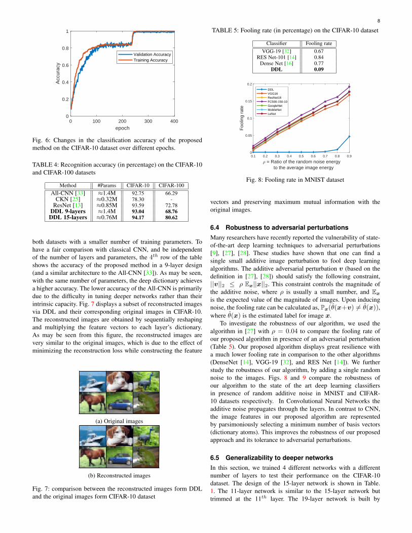
Fig. 6: Changes in the classification accuracy of the proposedmethod on the CIFAR-10 dataset over different epochs.

TABLE 4: Recognition accuracy (in percentage) on the CIFAR-10and CIFAR-100 datasets

Method #Params CIFAR-10 CIFAR-100All-CNN [33] ≈1.4M 92.75 66.29

CKN [25] ≈0.32M 78.30 -ResNet [13] ≈0.85M 93.59 72.78

DDL 9-layers ≈1.4M 93.04 68.76DDL 15-layers ≈0.76M 94.17 80.62

both datasets with a smaller number of training parameters. Tohave a fair comparison with classical CNN, and be independentof the number of layers and parameters, the 4th row of the tableshows the accuracy of the proposed method in a 9-layer design(and a similar architecture to the All-CNN [33]). As may be seen,with the same number of parameters, the deep dictionary achievesa higher accuracy. The lower accuracy of the All-CNN is primarilydue to the difficulty in tuning deeper networks rather than theirintrinsic capacity. Fig. 7 displays a subset of reconstructed imagesvia DDL and their corresponding original images in CIFAR-10.The reconstructed images are obtained by sequentially reshapingand multiplying the feature vectors to each layer’s dictionary.As may be seen from this figure, the reconstructed images arevery similar to the original images, which is due to the effect ofminimizing the reconstruction loss while constructing the feature

(a) Original images

(b) Reconstructed images

Fig. 7: comparison between the reconstructed images form DDLand the original images form CIFAR-10 dataset

TABLE 5: Fooling rate (in percentage) on the CIFAR-10 dataset

Classifier Fooling rateVGG-19 [32] 0.67

RES Net-101 [14] 0.84Dense Net [16] 0.77

DDL 0.09

0.1 0.2 0.3 0.4 0.5 0.6 0.7 0.8 0.9

= Ratio of the random noise energy to the average image energy

0

0.05

0.1

0.15

0.2

Foo

ling

rate

DDLVGG16ResNet18FC500-150-10GoogleNetMobileNetLeNet

Fig. 8: Fooling rate in MNIST dataset

vectors and preserving maximum mutual information with theoriginal images.

6.4 Robustness to adversarial perturbationsMany researchers have recently reported the vulnerability of state-of-the-art deep learning techniques to adversarial perturbations[9], [27], [28]. These studies have shown that one can find asingle small additive image perturbation to fool deep learningalgorithms. The additive adversarial perturbation v (based on thedefinition in [27], [28]) should satisfy the following constraint,||v||2 ≤ ρ Ex||x||2. This constraint controls the magnitude ofthe additive noise, where ρ is usually a small number, and Ex

is the expected value of the magnitude of images. Upon inducingnoise, the fooling rate can be calculated as, Px(θ(x+v) 6= θ(x)),where θ(x) is the estimated label for image x.

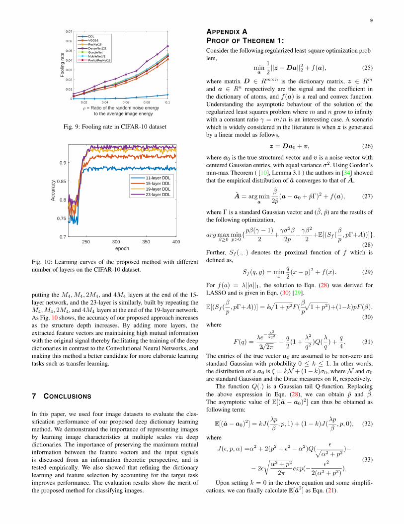
To investigate the robustness of our algorithm, we used thealgorithm in [27] with ρ = 0.04 to compare the fooling rate ofour proposed algorithm in presence of an adversarial perturbation(Table 5). Our proposed algorithm displays great resilience witha much lower fooling rate in comparison to the other algorithms(DenseNet [14], VGG-19 [32], and RES Net [14]). We furtherstudy the robustness of our algorithm, by adding a single randomnoise to the images. Figs. 8 and 9 compare the robustness ofour algorithm to the state of the art deep learning classifiersin presence of random additive noise in MNIST and CIFAR-10 datasets respectively. In Convolutional Neural Networks theadditive noise propagates through the layers. In contrast to CNN,the image features in our proposed algorithm are representedby parsimoniously selecting a minimum number of basis vectors(dictionary atoms). This improves the robustness of our proposedapproach and its tolerance to adversarial perturbations.

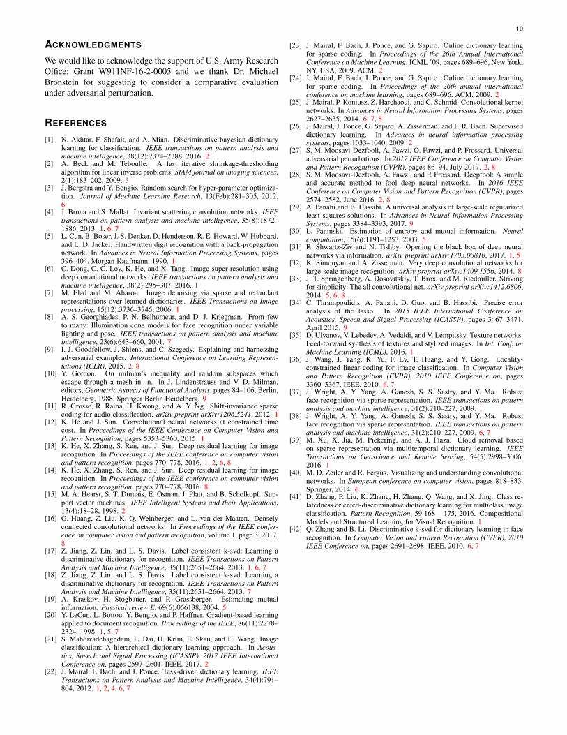
6.5 Generalizability to deeper networksIn this section, we trained 4 different networks with a differentnumber of layers to test their performance on the CIFAR-10dataset. The design of the 15-layer network is shown in Table.1. The 11-layer network is similar to the 15-layer network buttrimmed at the 11th layer. The 19-layer network is built by

9

0.02 0.04 0.06 0.08 0.1

= Ratio of the random noise energy to the average image energy

0

0.01

0.02

0.03

0.04

0.05

0.06

0.07

Foo

ling

rate

DDLVGG16ResNet18DenseNet121GoogleNetMobileNetV2PreActResNet18

Fig. 9: Fooling rate in CIFAR-10 dataset

250 300 350 400

epoch

0.7

0.75

0.8

0.85

0.9

Acc

urac

y

11-layer DDL15-layer DDL19-layer DDL23-layer DDL

Fig. 10: Learning curves of the proposed method with differentnumber of layers on the CIFAR-10 dataset.

putting the M4,M4, 2M4, and 4M4 layers at the end of the 15-layer network, and the 23-layer is similarly, built by repeating theM4,M4, 2M4, and 4M4 layers at the end of the 19-layer network.As Fig. 10 shows, the accuracy of our proposed approach increasesas the structure depth increases. By adding more layers, theextracted feature vectors are maintaining high mutual informationwith the original signal thereby facilitating the training of the deepdictionaries in contrast to the Convolutional Neural Networks, andmaking this method a better candidate for more elaborate learningtasks such as transfer learning.

7 CONCLUSIONS

In this paper, we used four image datasets to evaluate the clas-sification performance of our proposed deep dictionary learningmethod. We demonstrated the importance of representing imagesby learning image characteristics at multiple scales via deepdictionaries. The importance of preserving the maximum mutualinformation between the feature vectors and the input signalsis discussed from an information theoretic perspective, and istested empirically. We also showed that refining the dictionarylearning and feature selection by accounting for the target taskimproves performance. The evaluation results show the merit ofthe proposed method for classifying images.

APPENDIX APROOF OF THEOREM 1:Consider the following regularized least-square optimization prob-lem,

mina

1

2||z −Da||22 + f(a), (25)

where matrix D ∈ Rm×n is the dictionary matrix, z ∈ Rm

and a ∈ Rn respectively are the signal and the coefficient inthe dictionary of atoms, and f(a) is a real and convex function.Understanding the asymptotic behaviour of the solution of theregularized least squares problem where m and n grow to infinitywith a constant ratio γ = m/n is an interesting case. A scenariowhich is widely considered in the literature is when z is generatedby a linear model as follows,

z = Da0 + v, (26)

where a0 is the true structured vector and v is a noise vector withcentered Gaussian entries, with equal variance σ2. Using Gordon’smin-max Theorem ( [10], Lemma 3.1 ) the authors in [34] showedthat the empirical distribution of a converges to that of A,

A = arg mina

β

2p(a− a0 + pΓ)2 + f(a), (27)

where Γ is a standard Gaussian vector and (β, p) are the results ofthe following optimization,

argmaxβ≥0

minp>0{pβ(γ − 1)

2+γσ2β

2p−γβ

2

2+E[(Sf (

β

p, pΓ+A))]}.

(28)Further, Sf (., .) denotes the proximal function of f which isdefined as,

Sf (q, y) = minx

q

2(x− y)2 + f(x). (29)

For f(a) = λ||a||1, the solution to Eqn. (28) was derived forLASSO and is given in Eqn. (30) [29].

E[(Sf (β

p, pΓ+A))] = k

√1 + p2F (

β

p

√1 + p2)+(1−k)pF (β),

(30)where

F (q) =λe− λ2

2q2

2√

2π− q

2(1 +

λ2

q2)Q(

λ

q) +

q

4. (31)

The entries of the true vector a0 are assumed to be non-zero andstandard Gaussian with probability 0 ≤ k ≤ 1. In other words,the distribution of a a0 is ξ = kN + (1− k)σ0, where N and σ0

are standard Gaussian and the Dirac measures on R, respectively.The function Q(.) is a Gaussian tail Q-function. Replacing

the above expression in Eqn. (28), we can obtain p and β.The asymptotic value of E[(a − a0)2] can thus be obtained asfollowing term:

E[(a− a0)2] = kJ(λp

β, p, 1) + (1− k)J(

λp

β, p, 0), (32)

where

J(ε, p, α) =α2 + 2(p2 + ε2 − α2)Q(ε√

α2 + p2)−

− 2ε

√α2 + p2

2πexp(− ε2

2(α2 + p2)).

(33)

Upon setting k = 0 in the above equation and some simplifi-cations, we can finally calculate E[a2] as Eqn. (21).

10

ACKNOWLEDGMENTS

We would like to acknowledge the support of U.S. Army ResearchOffice: Grant W911NF-16-2-0005 and we thank Dr. MichaelBronstein for suggesting to consider a comparative evaluationunder adversarial perturbation.

REFERENCES

[1] N. Akhtar, F. Shafait, and A. Mian. Discriminative bayesian dictionarylearning for classification. IEEE transactions on pattern analysis andmachine intelligence, 38(12):2374–2388, 2016. 2

[2] A. Beck and M. Teboulle. A fast iterative shrinkage-thresholdingalgorithm for linear inverse problems. SIAM journal on imaging sciences,2(1):183–202, 2009. 3

[3] J. Bergstra and Y. Bengio. Random search for hyper-parameter optimiza-tion. Journal of Machine Learning Research, 13(Feb):281–305, 2012.6

[4] J. Bruna and S. Mallat. Invariant scattering convolution networks. IEEEtransactions on pattern analysis and machine intelligence, 35(8):1872–1886, 2013. 1, 6, 7

[5] L. Cun, B. Boser, J. S. Denker, D. Henderson, R. E. Howard, W. Hubbard,and L. D. Jackel. Handwritten digit recognition with a back-propagationnetwork. In Advances in Neural Information Processing Systems, pages396–404. Morgan Kaufmann, 1990. 1

[6] C. Dong, C. C. Loy, K. He, and X. Tang. Image super-resolution usingdeep convolutional networks. IEEE transactions on pattern analysis andmachine intelligence, 38(2):295–307, 2016. 1

[7] M. Elad and M. Aharon. Image denoising via sparse and redundantrepresentations over learned dictionaries. IEEE Transactions on Imageprocessing, 15(12):3736–3745, 2006. 1

[8] A. S. Georghiades, P. N. Belhumeur, and D. J. Kriegman. From fewto many: Illumination cone models for face recognition under variablelighting and pose. IEEE transactions on pattern analysis and machineintelligence, 23(6):643–660, 2001. 7

[9] I. J. Goodfellow, J. Shlens, and C. Szegedy. Explaining and harnessingadversarial examples. International Conference on Learning Represen-tations (ICLR), 2015. 2, 8

[10] Y. Gordon. On milman’s inequality and random subspaces whichescape through a mesh in n. In J. Lindenstrauss and V. D. Milman,editors, Geometric Aspects of Functional Analysis, pages 84–106, Berlin,Heidelberg, 1988. Springer Berlin Heidelberg. 9

[11] R. Grosse, R. Raina, H. Kwong, and A. Y. Ng. Shift-invariance sparsecoding for audio classification. arXiv preprint arXiv:1206.5241, 2012. 1

[12] K. He and J. Sun. Convolutional neural networks at constrained timecost. In Proceedings of the IEEE Conference on Computer Vision andPattern Recognition, pages 5353–5360, 2015. 1

[13] K. He, X. Zhang, S. Ren, and J. Sun. Deep residual learning for imagerecognition. In Proceedings of the IEEE conference on computer visionand pattern recognition, pages 770–778, 2016. 1, 2, 6, 8

[14] K. He, X. Zhang, S. Ren, and J. Sun. Deep residual learning for imagerecognition. In Proceedings of the IEEE conference on computer visionand pattern recognition, pages 770–778, 2016. 8

[15] M. A. Hearst, S. T. Dumais, E. Osman, J. Platt, and B. Scholkopf. Sup-port vector machines. IEEE Intelligent Systems and their Applications,13(4):18–28, 1998. 2

[16] G. Huang, Z. Liu, K. Q. Weinberger, and L. van der Maaten. Denselyconnected convolutional networks. In Proceedings of the IEEE confer-ence on computer vision and pattern recognition, volume 1, page 3, 2017.8

[17] Z. Jiang, Z. Lin, and L. S. Davis. Label consistent k-svd: Learning adiscriminative dictionary for recognition. IEEE Transactions on PatternAnalysis and Machine Intelligence, 35(11):2651–2664, 2013. 1, 6, 7

[18] Z. Jiang, Z. Lin, and L. S. Davis. Label consistent k-svd: Learning adiscriminative dictionary for recognition. IEEE Transactions on PatternAnalysis and Machine Intelligence, 35(11):2651–2664, 2013. 7

[19] A. Kraskov, H. Stogbauer, and P. Grassberger. Estimating mutualinformation. Physical review E, 69(6):066138, 2004. 5

[20] Y. LeCun, L. Bottou, Y. Bengio, and P. Haffner. Gradient-based learningapplied to document recognition. Proceedings of the IEEE, 86(11):2278–2324, 1998. 1, 5, 7

[21] S. Mahdizadehaghdam, L. Dai, H. Krim, E. Skau, and H. Wang. Imageclassification: A hierarchical dictionary learning approach. In Acous-tics, Speech and Signal Processing (ICASSP), 2017 IEEE InternationalConference on, pages 2597–2601. IEEE, 2017. 2

[22] J. Mairal, F. Bach, and J. Ponce. Task-driven dictionary learning. IEEETransactions on Pattern Analysis and Machine Intelligence, 34(4):791–804, 2012. 1, 2, 4, 6, 7

[23] J. Mairal, F. Bach, J. Ponce, and G. Sapiro. Online dictionary learningfor sparse coding. In Proceedings of the 26th Annual InternationalConference on Machine Learning, ICML ’09, pages 689–696, New York,NY, USA, 2009. ACM. 2

[24] J. Mairal, F. Bach, J. Ponce, and G. Sapiro. Online dictionary learningfor sparse coding. In Proceedings of the 26th annual internationalconference on machine learning, pages 689–696. ACM, 2009. 2

[25] J. Mairal, P. Koniusz, Z. Harchaoui, and C. Schmid. Convolutional kernelnetworks. In Advances in Neural Information Processing Systems, pages2627–2635, 2014. 6, 7, 8

[26] J. Mairal, J. Ponce, G. Sapiro, A. Zisserman, and F. R. Bach. Superviseddictionary learning. In Advances in neural information processingsystems, pages 1033–1040, 2009. 2

[27] S. M. Moosavi-Dezfooli, A. Fawzi, O. Fawzi, and P. Frossard. Universaladversarial perturbations. In 2017 IEEE Conference on Computer Visionand Pattern Recognition (CVPR), pages 86–94, July 2017. 2, 8

[28] S. M. Moosavi-Dezfooli, A. Fawzi, and P. Frossard. Deepfool: A simpleand accurate method to fool deep neural networks. In 2016 IEEEConference on Computer Vision and Pattern Recognition (CVPR), pages2574–2582, June 2016. 2, 8

[29] A. Panahi and B. Hassibi. A universal analysis of large-scale regularizedleast squares solutions. In Advances in Neural Information ProcessingSystems, pages 3384–3393, 2017. 9

[30] L. Paninski. Estimation of entropy and mutual information. Neuralcomputation, 15(6):1191–1253, 2003. 5

[31] R. Shwartz-Ziv and N. Tishby. Opening the black box of deep neuralnetworks via information. arXiv preprint arXiv:1703.00810, 2017. 1, 5

[32] K. Simonyan and A. Zisserman. Very deep convolutional networks forlarge-scale image recognition. arXiv preprint arXiv:1409.1556, 2014. 8

[33] J. T. Springenberg, A. Dosovitskiy, T. Brox, and M. Riedmiller. Strivingfor simplicity: The all convolutional net. arXiv preprint arXiv:1412.6806,2014. 5, 6, 8

[34] C. Thrampoulidis, A. Panahi, D. Guo, and B. Hassibi. Precise erroranalysis of the lasso. In 2015 IEEE International Conference onAcoustics, Speech and Signal Processing (ICASSP), pages 3467–3471,April 2015. 9

[35] D. Ulyanov, V. Lebedev, A. Vedaldi, and V. Lempitsky. Texture networks:Feed-forward synthesis of textures and stylized images. In Int. Conf. onMachine Learning (ICML), 2016. 1

[36] J. Wang, J. Yang, K. Yu, F. Lv, T. Huang, and Y. Gong. Locality-constrained linear coding for image classification. In Computer Visionand Pattern Recognition (CVPR), 2010 IEEE Conference on, pages3360–3367. IEEE, 2010. 6, 7

[37] J. Wright, A. Y. Yang, A. Ganesh, S. S. Sastry, and Y. Ma. Robustface recognition via sparse representation. IEEE transactions on patternanalysis and machine intelligence, 31(2):210–227, 2009. 1

[38] J. Wright, A. Y. Yang, A. Ganesh, S. S. Sastry, and Y. Ma. Robustface recognition via sparse representation. IEEE transactions on patternanalysis and machine intelligence, 31(2):210–227, 2009. 6, 7

[39] M. Xu, X. Jia, M. Pickering, and A. J. Plaza. Cloud removal basedon sparse representation via multitemporal dictionary learning. IEEETransactions on Geoscience and Remote Sensing, 54(5):2998–3006,2016. 1

[40] M. D. Zeiler and R. Fergus. Visualizing and understanding convolutionalnetworks. In European conference on computer vision, pages 818–833.Springer, 2014. 6

[41] D. Zhang, P. Liu, K. Zhang, H. Zhang, Q. Wang, and X. Jing. Class re-latedness oriented-discriminative dictionary learning for multiclass imageclassification. Pattern Recognition, 59:168 – 175, 2016. CompositionalModels and Structured Learning for Visual Recognition. 1

[42] Q. Zhang and B. Li. Discriminative k-svd for dictionary learning in facerecognition. In Computer Vision and Pattern Recognition (CVPR), 2010IEEE Conference on, pages 2691–2698. IEEE, 2010. 6, 7