Cut-cell Eta: Some history, and lessons from its present skill Fedor Mesinger 1, Katarina Veljovic 2

1) fedor.mesinger@sanu.ac.rs 2) katarina@ff.bg.ac.rs

Serbian Academy of Sciences and Arts, Belgrade, Serbia Faculty of Physics, Univ. of Belgrade, Serbia

Numerical Weather and Climate Modeling

Belgrade, Serbia, 10 September 2018

1973:  

However: How predictable is the weather ?

Earliest work on atmospheric “predictability”: Phil Thompson 1957 . . . accurate description of the initial state is simply impossible; Consequences?

“… two solutions … initial states that differ …”

“predictability time limit”: a bit more than a week

Skill ?

Breakthrough towards full understanding: Ed Lorenz (1963)

“chaos theory”

Small scale errors will grow also !

From: “The Essence of Chaos” (Lorenz 1993): “Chaos”1. The property that characterizes a dynamical system in which most orbits exhibit sensitivedependence; full chaos

Later: Lorenz (1917-2008), March 2006:

When the present determines the future but the approximate present

does not approximately determine the future

Chaos:

Acknowledgement: Posting on Eugenia Kalnay’s office door at the Univ. of Maryland

Accuracy of the jet stream position forecast as a dynamical core test: Cut-cell Eta vs. ECMWF 32-day

ensemble results

Accuracy ?  of a model, ran using real data IC

Issues: Atmosphere is chaotic

Results depend on data assimilation system

Impacts of both are avoided if we drive our limited area “test

model” by ICs and LBCs of an ensemble of a global model

“Although  spectral  transform  methods  are  being  predicted  to  be  phased  out,  the  current  spectral  model  at  the  European  Centre  for  Medium-­‐‑Range  Weather  Forecasts  …  is  the  

benchmark  to  beat,  and  it  is  not  clear  that  any  of  the  new  developments  are  ready  to  replace  it.”

 Côté  J,  Jablonowski  C,  Bauer  P,  Wedi  N  (2015)  Numerical  methods  of  the  atmosphere  and  ocean.  Seamless  predicJon  of  the  Earth  

system:  From  minutes  to  months,  101–124.  World  Meteorological  OrganizaJon,  WMO-­‐No.  1156.    

Forecast, Hits, and Observed (F, H, O) area, or number of model grid boxes:

O H

ab

c

d

F

Many verification scores. One:

�

ETS = H −E (H )F + O −H −E (H )

“Equitable Threat Score”

or, Gilbert (1884 !) Skill Score Bias = F / O  

Accuracy of the jet stream position . . . .  

ECMWF once a week runs a 51 member ensemble forecast 32

days ahead

Veljovic K, Rajkovic B, Fennessy MJ, Altshuler EL, Mesinger F (2010) Regional climate modeling: Should one attempt improving on the

large scales? Lateral boundary condition scheme: Any impact? Meteorol Zeitschrift, 19, 237-246, doi:10.1127/0941-2948/2010/0460

 Mesinger F, Chou SC, Gomes J, Jovic D, Bastos P, Bustamante JF,

Lazic L, Lyra AA, Morelli S, Ristic I, Veljovic K (2012) An upgraded version of the Eta model. Meteorol Atmos Phys 116, 63–79.

doi:10.1007/s00703-012-0182-z

Mesinger, F, Veljovic K (2017) Eta vs. sigma: Review of past results, Gallus-Klemp test, and large-scale wind skill in ensemble

experiments. Meteorol Atmos Phys, 129, 573-593, doi:10.1007/s00703-016-0496-3

To address the Gallus-Klemp (2000) problem: The sloping steps (a simple cut-cell scheme), vertical grid:

The central v box exchanges momentum, on its right side, with v boxes of two layers:

Horizontal treatment, 3D

Case #1: topography of box 1 is higher than those of 2, 3, and 4; “Slope 1”

Inside the central v box, topography descends from the center of T1 box down by one layer thickness, linearly, to the centers of T2, T3 and T4

Acknowledgements:  Dušan  Jović,  Jorge  Gomes  

How are grid cell values of topography obtained ?

Chop up each cell into n x n sub-cells;

Obtain each sub-cell mean value;

Obtain mean hm and silhouette cell value, round off to discrete interface value; Choose one depending on Laplacian hm Remove basins with all corner winds blocked;

Some more common sense rules (no waterfalls, do not close major ridges by silhouetting), but no smoothing

8 km horizontal resolution,

W/E profile at the latitude of about

the highest elevation of the

Andes 30 hr forecast:

NCAR graphics, no cell values

smoothing

Another  cut-­‐cell  scheme:  Steppeler  et  al.  (2008,  2013):    

Steppeler  J,  Park  S-­‐‑H,  Dobler  A  (2013)  Forecasts  covering  one  month  using  a  cut-­‐‑cell  model.  Geosci.  Model  Dev.,  6,  875-­‐‑882.  doi:10.5194/gmd-­‐‑6-­‐‑875-­‐‑2013

Verification results 21 ensemble members

Bias adjusted

ETS scores of wind

speeds > 45 m s-1, at 250

hPa, with respect to ECMWF analyses

ETSa:

More is better !

 

0 2 4 6 8 10 12 14 16 18 20 22 24 26 28 30 32Time (days)

0

0.2

0.4

0.6

0.8

Cumulative ETSa, 21 ensemble members

Eta

EC

ETSa

RMS wind difference of 250 hPa winds, with respect to ECMWF analyses

RMS:

Less is better !

 

0 2 4 6 8 10 12 14 16 18 20 22 24 26 28 30 32Time (days)

0

5

10

15

20

25Cumulative RMS difference, 21 members

Eta

EC RMS

What ingredient of the Eta is responsible for the advantage in scores ?

(It is not resolution, the first 10 days

resolution of two models was about the same)

0 2 4 6 8 10 12 14 16 18 20 22 24 26 28 30 32Time (days)

0

0,2

0,4

0,6

0,8

Cumulative ETSa, 21 ensemble members

0 2 4 6 8 10 12 14 16 18 20 22 24 26 28 30 32Time (days)

0

5

10

15

20

25Cumulative RMS difference, 21 members

21 members ran using Eta/sigma :

What was going on at about day 2-6 time ?    

   The  plot  Jmes  correspond  to  day  

3.0,  and  4.5,  respecJvely,  of  the  plots  of  the  two  preceding  slides  

 

Why was the Eta so much more accurate at this time ?

Ensemble average, 21 members, at 4.5 day time: Eta/sigma top left, Eta top right, EC driver bottom left, EC verification analysis bottom right.

Ета/σ Ета/η

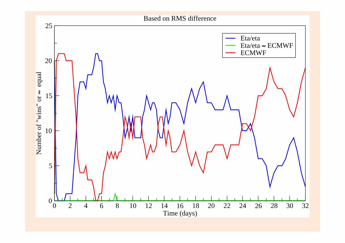
Another way of comparing model skill

as a function of time: number of “wins”

0 2 4 6 8 10 12 14 16 18 20 22 24 26 28 30 32Time (days)

0

5

10

15

20

25N

umbe

r of "

win

s" o

r ≈ e

qual

Eta/eta Eta/eta ≈ ECMWFECMWF

Based on ETSa

Four times from day 2.25 to day 4.5 every single Eta ensemble member, all 21 of them, had “jet stream” placed more accurately than their ECMWF driver members !

0 2 4 6 8 10 12 14 16 18 20 22 24 26 28 30 32Time (days)

0

5

10

15

20

25

Num

ber o

f "w

ins"

or ≈

equ

al

Eta/etaEta/eta ≈ Eta/sigmaEta/sigma

Based on ETSaEta vs. Eta/ sigma:

0 2 4 6 8 10 12 14 16 18 20 22 24 26 28 30 32Time (days)

0

5

10

15

20

25

Num

ber o

f "w

ins"

or ≈

equ

alEta/eta Eta/eta ≈ ECMWFECMWF

Based on RMS difference

0 2 4 6 8 10 12 14 16 18 20 22 24 26 28 30 32Time (days)

0

5

10

15

20

25

30

Num

ber o

f "w

ins"

or ≈

equ

al

Eta/eta Eta/eta ≈ ECMWFECMWF

Based on EDS (250 mb wind > 45 m/s)Based on the

Extreme Dependency Score (EDS), designed for forecasts of rare binary-

events (Stephenson

et al., Meteor. Appl. 2008)

So far we looked at score numbers, and average maps of 21

members

Now: Contours of all 21 members of areas

of wind speeds > 45 m/s

Conclusions • Strong evidence that coordinate systems intersecting topography are able to perform

significantly better than terrain-following systems; (in  agreement  with  Steppeler  et  al.  2013)

PGF repair effort does exist (Zängl  MWR  2012)  does  it  remove  the  problems  shown  ?

Conclusions • The Eta must have additional components

responsible for its increased accuracy against ECMWF

Candidate reasons:  

•    Arakawa  horizontal  advecJon  scheme  (Janjić  1984);    

•    Finite-­‐volume  van  Leer  type  verJcal  advecJon  of  all  variables  (Mesinger  and  Jovic  2002);      

•    Very  careful  construcJon  of  model  topography  (MY2017),  with  grid  cell  values  selected  between  their  mean  and  silhouege  values,  depending  on  surrounding  values,  and  no  smoothing;    

•    Exact  conservaJon  of  energy  in  space  differencing  in  transformaJon  between  the  kineJc  and  potenJal  energy;    

•    .  .  .  .  .  .