Aquaculture 358–359 (2012) 23–34

Contents lists available at SciVerse ScienceDirect

Aquaculture

j ourna l homepage: www.e lsev ie r .com/ locate /aqua-on l ine

Cultivation of gilthead bream in monoculture and integrated multi-trophicaquaculture. Analysis of production and environmental effects by means ofthe FARM model

J.G. Ferreira a,⁎, C. Saurel a, J.M. Ferreira b,c

a New University of Lisbon, Faculty of Sciences and Technology, Centre for Ocean and Environment, DCEA, FCT, Qta Torre, 2829-516 Monte de Caparica, Portugalb Departamento de Física, Universidade de Trás-os-Montes e Alto Douro, 5001-801 Vila Real, Portugalc Centro de Física Atómica da Universidade de Lisboa, Departamento de Física da Faculdade de Ciências, Av. Prof. Gama Pinto 2, 1649-003 Lisboa, Portugal

⁎ Corresponding author.E-mail address: joao@hoomi.com (J.G. Ferreira).

0044-8486/$ – see front matter © 2012 Elsevier B.V. Alldoi:10.1016/j.aquaculture.2012.06.015

a b s t r a c t

a r t i c l e i n f o

Article history:Received 3 January 2012Received in revised form 12 June 2012Accepted 15 June 2012Available online 27 June 2012

Keywords:Gilthead breamPond and offshore cultureFinfish and shellfish IMTACarrying capacitySite selectionFARM model

The aquaculture growth required to meet increasing protein demand by a growing world population,predicted to reach 9 billion people by 2050, is driving innovation in both siting and culture practice. Limitedpossibilities for expansion on land and in inshore coastal areas, and technological improvements in farmingstructures, have led to widespread interest in offshore aquaculture.A gilthead bream (Sparus aurata) model has been developed and integrated with existing shellfish models inthe Farm Aquaculture Management System (FARM) model, in order to analyse various aspects of onshore andoffshore aquaculture. The FARM model was used to compare the quantitative effects of finfish monoculturewith Integrated Multi-Trophic Aquaculture (IMTA) in ponds, in terms of production, environmental external-ities, and economic performance. Very clear benefits of IMTA could be seen in the comparison. The same ap-proach was then applied to offshore culture, considering a combination of gilthead in cages and Pacific oyster(Crassostrea gigas) suspended from longlines. For offshore culture, the primary production and diagenesismodules of FARM were switched off, since there are no feedbacks from those processes to the farm area. Ex-cept in upwelling areas, the concentration of food drivers for filter-feeding shellfish falls markedly with dis-tance from the shore―simulations with FARM suggest that in food-poor areas, co-cultivation of bivalves withfish can significantly improve shellfish production, and that the distribution of finfish can be optimised to re-duce shellfish food depletion in the inner parts of the farm. We calculate the environmental benefits of IMTAboth in terms of population-equivalents and the potential for nutrient credit trading. The finfish model inte-grated in FARM deals explicitly with the metabolic energy cost of opposing offshore currents in cage culture,and a model analysis suggests that gilthead cultivation at current speeds in the range of 0.1 to 0.5 m s−1 isoptimal. The lower end of that spectrum probably translates into a greater deviation from the fillet qualityobtained from wild fish, and above that limit there is a rapid increase of the feed conversion ratio (FCR)and cultivation becomes financially unattractive.

© 2012 Elsevier B.V. All rights reserved.

1. Introduction

Marine finfish aquaculture in Europe is dominated by two majorspecies, Atlantic salmon (Salmo salar) in the north, with an annual pro-duction of almost 900,000 t (EC Fisheries, 2011), and gilthead bream(Sparus aurata) in the south, with an estimated production (2008) ofalmost 129,000 t y−1 (FEAP, 2009). In both cases, as well as for speciessuch as the European sea bass Dicentrarchus labrax, which is cultivatedin smaller quantities, the market acceptance of the cultivated productis high (e.g. Verbeke et al., 2007), and wild-captured fish are often

rights reserved.

available only at premium prices that are inaccessible to mostconsumers.

Two important developments are currently occurring in Europeand North America, driven by competition for marine space and byincreased environmental awareness (Olesen et al., 2010). The first isan increased interest in offshore aquaculture (Aguilar-Manjarrez etal., 2008), made possible through improvements in culture structures,and the second is the co-cultivation of different trophic groups in In-tegrated Multi-Trophic Aquaculture (IMTA, e.g. Chopin et al., 2010;Neori et al., 2004; Troell et al., 2009).

In the first case, there are a number of potential benefits in placingculture structures such as sea cages some distance from the shore, re-ducing visual impacts (Byron and Costa-Pierce, 2010; Byron et al.,2011), and promoting greater dispersion ofwaste products and uneaten

24 J.G. Ferreira et al. / Aquaculture 358–359 (2012) 23–34

food, by taking advantage of stronger hydrodynamics and greaterwatercolumn depth (see Holmer, 2010, for a review). The disadvantagesinclude higher operating costs and potentially lower yields at highercurrent speeds (Kapetsky et al., 2012).

Allied to the social and environmental carrying capacity advan-tages of cultivating finfish further out to sea, is the possibility ofco-cultivation with bivalve shellfish in longlines or rafts in IMTA (e.g.Ferreira et al., 2010, 2011). The additional food supply to speciessuch as mussels and oysters may to some extent compensate for themore oligotrophic nature of offshore waters, and will reduce the envi-ronmental footprint of finfish culture, while providing an extra cashcrop for the farmer.

IMTA was documented thousands of years ago in China (Moo,undated), and has been standard practice in SE Asia for hundreds ofyears (Ferreira et al., in press), but the effectiveness of multi-trophicculture has been shown mainly in inland pond culture, e.g. by com-bining shrimp or fish with razor clams, together with a primary pro-ducer such as water spinach (Ipomoea aquatica). It is more difficultto establish the practical consequences of IMTA in open water, dueto hydrodynamic effects, except in situations where the cultivationintensity at the whole-bay scale turns embayments or estuaries intothe equivalent of a pond. Such high-density culture is widespread inChina; for instance in Sanggou Bay (Zhang et al., 2009), an annualproduction of 150,000 t of kelp, shellfish, and finfish is documentedfor an area of 140 km2 (Ferreira et al., 2008a).

Although the importance of IMTA is increasingly recognised inNorth America and Europe, it is effectively practised only in a fewfarms in Canada (Cross, pers. com.), and the cultivation densitiesare characteristic of aquaculture in the western world, i.e. they arepresently too low to allow the environmental benefits to be easilyquantified.

Mathematical models have been applied to analyse the productionand environmental effects of finfish cultivation (e.g. Corner et al.,2006; Cromey et al., 2002; Skogen et al., 2009; Stigebrandt et al.,2004), and have likewise been used to predict the yield, environmentalimpact, and economic optimisation of shellfish farming operations (e.g.Brigolin et al., 2009; Chamberlain, 2002; Ferreira et al., 2009; Giles etal., 2009), but the combined production and effects of finfish and shell-fish cultivations in IMTA have not to our knowledge been modelledpreviously, either in ponds or open water farms.

This work aims to develop and test an integrated modellingapproach for IMTA of finfish and shellfish, both at the pond scale andin offshore conditions. This combination has been implemented in theFARM model (e.g. Ferreira et al., 2011; Silva et al., 2011), and usesgilthead bream and Pacific oysters (Crassostrea gigas) as test speciesfor co-cultivation.

The main objectives are:

1. To examine the production, environmental effects, and economicexternalities of monoculture of gilthead bream in ponds, and com-pare this to IMTA with oysters.

2. To extend this analysis to offshore farms, taking into account boththe variation in current speed and the effects of co-cultivation offinfish on oyster growth.

3. To illustrate howmodels of this nature can assist in supporting siteselection, from the standpoints of production, environment, andeconomic viability.

2. Methodology

The models applied in this work were developed, tested, and com-bined using a stepwise approach, building on an existing framework.The sequence was:

• development or adaptation of individual models, using the simplestset of formulations that allowed for an analysis of feeding, growth,metabolism, and environmental effects;

• integration of individual growth models into a population dynamicsframework (see e.g. Nunes et al., 2011), enabling themodels to provideresults on the marketable cohorts of finfish and shellfish, in orderto focus on the harvestable biomass of interest to producers;population-scale modelling also allowed for food consumption andenvironmental effects to be simulated at the culture scale;

• simulation of the physical systems where the cultivated species aregrown. In the case of pond culture this requires a simulation ofsediment diagenesis, whereas in open water the approach previ-ously developed in FARM (e.g. Ferreira et al., 2007) was used,with the additional module for biodeposition described in Silva etal. (2011).

The main methodological innovations were the simulation ofgrowth for gilthead, and the implementation of the diagenesis compo-nent. These are described in more detail below.

2.1. Individual model for gilthead bream

Several models already exist for individual growth of giltheadbream (e.g. Brigolin et al., 2010; Hernández et al., 2003; Libralatoand Solidoro, 2008); therefore where possible, we drew on formula-tions already tested by those authors. However, we required anexplicit simulation of feeding (see below), and we additionally neededto fraction the various components of metabolism in order to simulategrowth at different current speeds.

The individual growth model developed (AquaFish) is based on netenergy balance, and uses a similar rationale (i.e. maximum simplicity)to the AquaShell model developed for bivalves (Ferreira et al., 2010;Silva et al., 2011). By contrast to organically extractive shellfish aqua-culture, finfish are fed (dry feed pellets in the West but often trashfish in SE Asia)—one of the key indicators of finfish aquaculture is thefeed conversion ratio, or FCR, so the feed supplied must be accountedfor in the model.

Another key difference in simulating feeding is that aconcentration-based approach, as is normally used in shellfish models,is not appropriate, since gilthead (and other fish species such as salmonand bass) eat a ‘meal’; this is best thought of by considering that in thewild, gilthead thrive on a diet of discrete prey items such as mussels,crustaceans, and smaller fish.

2.1.1. Feeding and digestionElliott and Persson (1978) derived various equations to represent

food consumption and gastric evacuation in fish. We have used a sim-ilar approach in developing a feeding model, following also from theequations given in Franco et al. (2006).

Themaximum food intake (g DWpellets d−1) into thefish stomachis calculated based on allometry (Brigolin et al., 2010), and thetemperature effect (fθ) on feeding (Eq. (1)) follows Hernández et al.(2003):

f θ ¼ D eα θm−θð Þ−eβ θm−θð Þ� �ð1Þ

where (values from Hernández et al., 2003):

θ water temperature (°C)θm maximum lethal temperature=32.9 °Cα temperature function parameter=–0.12 °C−1

β temperature function parameter=−0.15 °C−1

D temperature adjustment parameter=4.93.

Feeding is a function of stomach volume, converted to dry mass offeed pellets, and of stomach ‘fullness’; the feeding rate is reducedthrough the application of a satiation coefficient as the animal's stomachcapacity is reached. Fish stomach capacity has been studied by e.g. Knight

25J.G. Ferreira et al. / Aquaculture 358–359 (2012) 23–34

and Magraf (1982), and Gosch et al. (2009). In AquaFish, stomachcapacity is governed by allometry, after Gosch et al. (2009). Since nodata were available for gilthead, an equation for spotted bass (Eq. (2))was used:

Sv ¼ 3:587� 10−8L3:514 ð2Þ

where:

Sv stomach volume (ml)L fish length (mm).

Sv was converted to dry mass using the pellet density. Giltheadlength (L) was calculated from biomass (W) following Wassef andShehata (1990):

Log W ¼ −2:1724þ 3:2216 Log L: ð3Þ

Jobling (1981) provides a detailed review of the different equa-tions for gastric evacuation in fish, of which the first-order decaymodel (Eq. (4)) appears to be the most realistic. Note that this equa-tion does not include the feeding component described earlier, i.e. itapplies for the period when no feeding occurs.

dScdt

¼ −γSc0:5 ð4Þ

where:

Sc volumetric stomach content (converted to mass, i.e. ρSc)and therefore using the mass or volume of the stomachcontent is irrelevant (g DW);

γ proportionality constant (calibrated to 1.5).

Food entering the gut through gastric evacuation is either assimi-lated or eliminated as faeces (Eq. (5)):

dGc

dt¼ dSc

dt−εFr−φGc ð5Þ

where:

Gc gut content (DW food)ε assimilation efficiency (no units)Fr feeding rate (g DW d−1)φ faecal elimination rate (g DW d−1).

Stomach content g DW

Days since sta

0

0.05

0.1

0.15

0.2

0.25

0.3

0.35

1 2 3 4 5

Sto

mac

h co

nten

t (g

DW

)

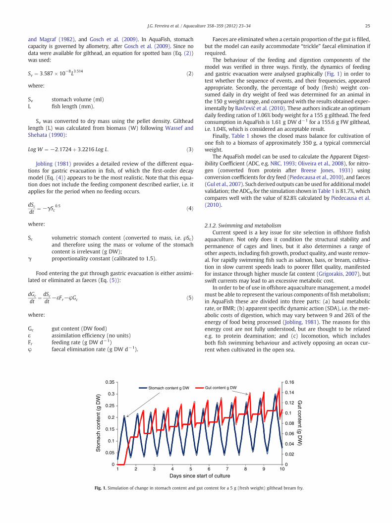
Fig. 1. Simulation of change in stomach content and gut

Faeces are eliminated when a certain proportion of the gut is filled,but the model can easily accommodate “trickle” faecal elimination ifrequired.

The behaviour of the feeding and digestion components of themodel was verified in three ways. Firstly, the dynamics of feedingand gastric evacuation were analysed graphically (Fig. 1) in order totest whether the sequence of events, and their frequencies, appearedappropriate. Secondly, the percentage of body (fresh) weight con-sumed daily in dry weight of feed was determined for an animal inthe 150 gweight range, and comparedwith the results obtained exper-imentally by Bavčević et al. (2010). These authors indicate an optimumdaily feeding ration of 1.06% body weight for a 155 g gilthead. The feedconsumption in AquaFish is 1.61 g DW d−1 for a 155.6 g FW gilthead,i.e. 1.04%, which is considered an acceptable result.

Finally, Table 1 shows the closed mass balance for cultivation ofone fish to a biomass of approximately 350 g, a typical commercialweight.

The AquaFish model can be used to calculate the Apparent Digest-ibility Coefficient (ADC, e.g. NRC, 1993; Oliveira et al., 2008), for nitro-gen (converted from protein after Breese Jones, 1931) usingconversion coefficients for dry feed (Piedecausa et al., 2010), and faeces(Gul et al., 2007). Such derived outputs can be used for additionalmodelvalidation; the ADCN for the simulation shown in Table 1 is 81.7%, whichcompares well with the value of 82.8% calculated by Piedecausa et al.(2010).

2.1.2. Swimming and metabolismCurrent speed is a key issue for site selection in offshore finfish

aquaculture. Not only does it condition the structural stability andpermanence of cages and lines, but it also determines a range ofother aspects, including fish growth, product quality, andwaste remov-al. For rapidly swimming fish such as salmon, bass, or bream, cultiva-tion in slow current speeds leads to poorer fillet quality, manifestedfor instance through higher muscle fat content (Grigorakis, 2007), butswift currents may lead to an excessive metabolic cost.

In order to be of use in offshore aquaculture management, a modelmust be able to represent the various components of fish metabolism;in AquaFish these are divided into three parts: (a) basal metabolicrate, or BMR; (b) apparent specific dynamic action (SDA), i.e. the met-abolic costs of digestion, which may vary between 9 and 26% of theenergy of food being processed (Jobling, 1981). The reasons for thisenergy cost are not fully understood, but are thought to be relatede.g. to protein deamination; and (c) locomotion, which includesboth fish swimming behaviour and actively opposing an ocean cur-rent when cultivated in the open sea.

Gut content g DW

rt of culture

Gut content (g D

W)

0

0.02

0.04

0.06

0.08

0.1

0.12

0.14

0.16

6 7 8 9 10

content for a 5 g (fresh weight) gilthead bream fry.

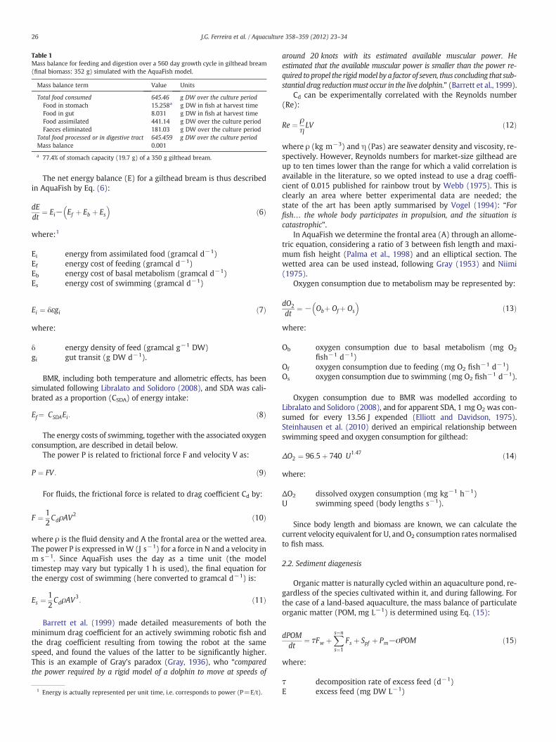
Table 1Mass balance for feeding and digestion over a 560 day growth cycle in gilthead bream(final biomass: 352 g) simulated with the AquaFish model.

Mass balance term Value Units

Total food consumed 645.46 g DW over the culture periodFood in stomach 15.258a g DW in fish at harvest timeFood in gut 8.031 g DW in fish at harvest timeFood assimilated 441.14 g DW over the culture periodFaeces eliminated 181.03 g DW over the culture period

Total food processed or in digestive tract 645.459 g DW over the culture periodMass balance 0.001

a 77.4% of stomach capacity (19.7 g) of a 350 g gilthead bream.

26 J.G. Ferreira et al. / Aquaculture 358–359 (2012) 23–34

The net energy balance (E) for a gilthead bream is thus describedin AquaFish by Eq. (6):

dEdt

¼ Ei− Ef þ Eb þ Es� �

ð6Þ

where:1

Ei energy from assimilated food (gramcal d−1)Ef energy cost of feeding (gramcal d−1)Eb energy cost of basal metabolism (gramcal d−1)Es energy cost of swimming (gramcal d−1)

Ei ¼ δεgi ð7Þ

where:

δ energy density of feed (gramcal g−1 DW)gi gut transit (g DW d−1).

BMR, including both temperature and allometric effects, has beensimulated following Libralato and Solidoro (2008), and SDA was cali-brated as a proportion (CSDA) of energy intake:

Ef¼ CSDAEi: ð8Þ

The energy costs of swimming, together with the associated oxygenconsumption, are described in detail below.

The power P is related to frictional force F and velocity V as:

P ¼ FV : ð9Þ

For fluids, the frictional force is related to drag coefficient Cd by:

F ¼ 12CdρAV

2 ð10Þ

where ρ is the fluid density and A the frontal area or the wetted area.The power P is expressed inW (J s−1) for a force in N and a velocity inm s−1. Since AquaFish uses the day as a time unit (the modeltimestep may vary but typically 1 h is used), the final equation forthe energy cost of swimming (here converted to gramcal d−1) is:

Es ¼12CdρAV

3: ð11Þ

Barrett et al. (1999) made detailed measurements of both theminimum drag coefficient for an actively swimming robotic fish andthe drag coefficient resulting from towing the robot at the samespeed, and found the values of the latter to be significantly higher.This is an example of Gray's paradox (Gray, 1936), who “comparedthe power required by a rigid model of a dolphin to move at speeds of

1 Energy is actually represented per unit time, i.e. corresponds to power (P=E/t).

around 20 knots with its estimated available muscular power. Heestimated that the available muscular power is smaller than the power re-quired to propel the rigidmodel by a factor of seven, thus concluding that sub-stantial drag reductionmust occur in the live dolphin.” (Barrett et al., 1999).

Cd can be experimentally correlated with the Reynolds number(Re):

Re ¼ ρηLV ð12Þ

where ρ (kg m−3) and η (Pas) are seawater density and viscosity, re-spectively. However, Reynolds numbers for market-size gilthead areup to ten times lower than the range for which a valid correlation isavailable in the literature, so we opted instead to use a drag coeffi-cient of 0.015 published for rainbow trout by Webb (1975). This isclearly an area where better experimental data are needed; thestate of the art has been aptly summarised by Vogel (1994): “Forfish… the whole body participates in propulsion, and the situation iscatastrophic”.

In AquaFish we determine the frontal area (A) through an allome-tric equation, considering a ratio of 3 between fish length and maxi-mum fish height (Palma et al., 1998) and an elliptical section. Thewetted area can be used instead, following Gray (1953) and Niimi(1975).

Oxygen consumption due to metabolism may be represented by:

dO2

dt¼ − Obþ Ofþ Os

� �ð13Þ

where:

Ob oxygen consumption due to basal metabolism (mg O2

fish−1 d−1)Of oxygen consumption due to feeding (mg O2 fish−1 d−1)Os oxygen consumption due to swimming (mg O2 fish−1 d−1).

Oxygen consumption due to BMR was modelled according toLibralato and Solidoro (2008), and for apparent SDA, 1 mg O2 was con-sumed for every 13.56 J expended (Elliott and Davidson, 1975).Steinhausen et al. (2010) derived an empirical relationship betweenswimming speed and oxygen consumption for gilthead:

ΔO2 ¼ 96:5þ 740 U1:47 ð14Þ

where:

ΔO2 dissolved oxygen consumption (mg kg−1 h−1)U swimming speed (body lengths s−1).

Since body length and biomass are known, we can calculate thecurrent velocity equivalent for U, and O2 consumption rates normalisedto fish mass.

2.2. Sediment diagenesis

Organic matter is naturally cycled within an aquaculture pond, re-gardless of the species cultivated within it, and during fallowing. Forthe case of a land-based aquaculture, the mass balance of particulateorganic matter (POM, mg L−1) is determined using Eq. (15):

dPOMdt

¼ τFw þXs¼n

s¼1

Fs þ Spf þ Pm−σPOM ð15Þ

where:

τ decomposition rate of excess feed (d−1)E excess feed (mg DW L−1)

27J.G. Ferreira et al. / Aquaculture 358–359 (2012) 23–34

S cultivated species (1 to n)Fs faecal contribution of species s (mg DW L−1 d−1)Spf bivalve shellfish pseudofaeces (mg DW L−1 d−1)Pm phytoplankton mortality (mg DW L−1 d−1)σ sedimentation rate of POM (d−1), determined using Stokes'

equation.

The mass balance equation for particulate organic nitrogen (PON)in the sediment is (Di Toro, 2001):

HdPONdt

¼ JPON−kPONHPON−wPONPON ð16Þ

where:

H sediment height (m)JPON flux of PON to sediment (mg N m−2 d−1)kPON 0.03 d−1 (Cartaxana and Catarino, 1997, 2002)wPON loss rate to sediment (burial) (m d−1).

Sediment diagenesis is calculated following Di Toro (2001) andSimas and Ferreira (2007). Eq. (17) represents the mineralisation ofsediment PON to ammonium and the flux of ammonium to the watercolumn.

HdNH4ðsedÞdt

¼ kPONHPON þ kLws NH4 watð Þ�NH4 sedð Þ� �

−wNH4NH4ðsedÞð17Þ

where:

NH4(sed) ammonium in sediment (mg N m−3)NH4(water) ammonium in water (mg N m−3)PON particulate organic nitrogen in sediment (mg N m−3)kLws 0.00017 m d−1

wNH4 0.0007 m d−1.

The ammonium that is returned to the water column, togetherwith that excreted by the cultivated organisms, and nitrogen inflowsthrough water intake, is used to determine primary production. Inopen water farms, pelagic primary production is neglected, due tothe short residence time of water in the farm, and the effects of sedi-ment diagenesis are only considered to establish the benthic footprintof the farm. Incorporation of both these processes in open waterfarms requires a system-scale modelling approach (e.g. Ferreira etal., 2008b; Nobre et al., 2010).

2.3. Oxygenation

Dissolved oxygen (DO) plays a key role in both the growth and sur-vival of cultivated species, and the water quality in ponds. The massbalance equation for DO contains terms for biological sources (primaryproduction) and sinks (e.g. finfish respiration), together with physicalcomponents, which can be divided into natural aeration, artificial aera-tion, and water exchange.

Natural aeration of ponds is simulated as a function of the DO satu-ration in the water and atmosphere, and turbulent mixing at the air/water interface, following Chapra (1997) and Nobre et al. (2005),using a Schmidt number of 500. A default wind speed of 2 m s−1 isset, but a climatological time series of wind speeds can be defined bythe model user.

Most cultivated ponds are subject to artificial aeration, thereforeFARM allows the user to specify three aeration regimes: (i) no artifi-cial aeration; (ii) optimised aeration; and (iii) constant aeration. If theculture pond has oxygen problems, selecting constant aeration willturn on the aerators at dusk (the full photoperiod for any latitude is

simulated in the model) in order to maximise efficiency andminimiseenergy costs. Aerators will be switched off as soon as 100% saturationis attained. If optimised aeration is preferred, it is triggered wheneverDO saturation falls below a user-defined threshold, and turned offwhen the value in the pond is above the threshold at dawn. The oper-ation of aerators (Eq. (18)) is simulated following Boyd (1998, 2009)and Tucker (2005).

OTR ¼ SOTRCs�Cp

9:091:024T−20ω ð18Þ

where:

OTR oxygen transfer rate in pond water (kg O2 h−1)SOTR standard oxygen transfer rate. In FARM this is determined

from the relationship between the standard aeration effi-ciency (SAE) and the horsepower of the aerator.

Cs DO at 100% saturation (mg L−1)Cp DO in pond (mg L−1)T water temperature (°C)ω oxygen transfer coefficient ratio.

In order to determine aquaculture production costs, the modeluser may specify the unit cost of electricity, or use the default valuesupplied. DO is considered to affect both growth and mortality, andit is possible to switch off those effects in FARM to examine the sen-sitivity of the cultivation to this variable. Primary production mayalso be switched off, to look at the ecosystem service provided byalgae in reoxygenating the pond water.

2.4. Model implementation

Component parts of the individual model for gilthead weretested and assembled in PowersimTM, a visual modelling platform.The complete model was then ported to C++, and implementedin object-oriented (OOP) code. Mass balance outputs were verifiedagainst the visual platform. Subsequently, the individual modelwas used to determine the scope for growth for a fish population,using well-tested equations (e.g. Ferreira et al., 2008b). Tenweight classes were used for the population model, ranging from0 to 460 g. The full model, capable of simulating fish growth andenvironmental effects both at the individual and population levels,was inserted into FARM, in the context of both land-based andopen water cultures. FARM simulates physical and chemical pro-cesses in both environments, together with shellfish growth andenvironmental effects. The combination of the various compo-nents into a modelling system was used as a tool for analysis ofmonoculture versus IMTA, and of the performance of offshoreaquaculture.

3. Results and discussion

A brief analysis of the individual finfish model is presented,followed by the results of the full application of finfish and shellfishmodels in an integrated framework, both for onshore and offshorecultures.

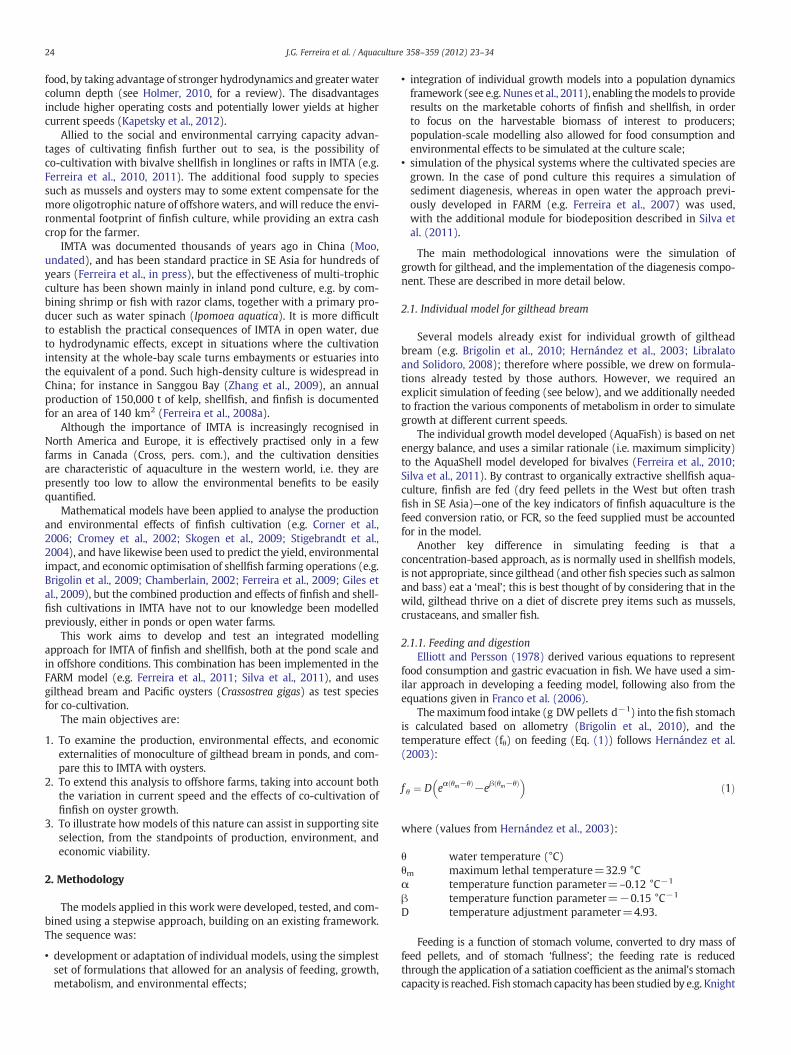
3.1. Individual finfish model

Fig. 2 shows the full mass balance for the growth of a 5 g giltheadfry to a weight of 350 g, over a 414 day culture period, at a tempera-ture range centred around 20 °C. The FCR is 1.3, which is under-estimated because the individual AquaFish model does not considerother processes typical of the farm itself (and which are simulated inthe final models) such as loss of pellets through deposition. Wastefeed in AquaFish is generated only by the animal's incapacity to eat

Food ingestion449 g DW

Respiration0.78 kg O2

Digestion in the gut

Faeces126 g DW

Feed supplied

463 g DW

Feed loss

14 g DW

Organic pollution

140 g DW

Urine7.4 g NH4

Inorganic pollution

7.4 g NH4

Energy assimilated

385 kcal

Cultivation:414 daysCurrent: 10 cm s-1

Biomass: 350 g FWLength: 29 cmFCR: 1.3ADC (N): 82%

Anabolism: 1471 kcalBMR: 277 kcalSDA: 809 kcalSwimming: 0.2 kcal

Fig. 2. Mass balance for individual growth of a gilthead bream (350 g final weight). Market sized bream do not normally reach sexual maturity, so the model does not account forreproduction. Gilthead image source: http://www.archive.org/details/histoirenaturell141255cuvi.

28 J.G. Ferreira et al. / Aquaculture 358–359 (2012) 23–34

all the food offered. Complementary cultivation parameters calculatedby the model for this example are: specific growth rate (SGR): 1.03%(ln) g d−1, and a thermal growth coefficient (TGC3, e.g. Jobling,2003) of 0.37 g1/3 °C−1.

The individual model was validated against measured data froman experimental aquaculture station in southern Portugal (F. Soares,pers. com). Measured biomass after 134 days was 303 (±69) g, and367 (±51) g after 246 days. The model results were 277 g and396 g, respectively. AquaFish was also tested against growth datafrom a farm in Turkey (Yilmaz and Arabaci, 2010). The model isable to reproduce the endpoint individual biomass of 337 g, at amean temperature of 19 °C, and determines a cultivation period of338 days. The experimental culture took place between January 1stand December 5th 2006, i.e. 339 days. The farm yields and themodel have an identical SGR, and the TGC3 coefficients differ by lessthan 2%.

0

500

1000

1500

2000

2500

3000

0.1 0.2 0.3 0.4 0.5

Cultivation period re

Oxygen consumed

FCR

Current spe

Cul

tivat

ion

perio

d (d

ays)

Best FCR and O2,Lower fillet quality

Cultivation period and FCR similar to

A, up to 6X O2

consumed relative to A, better quality

Inp

A B C

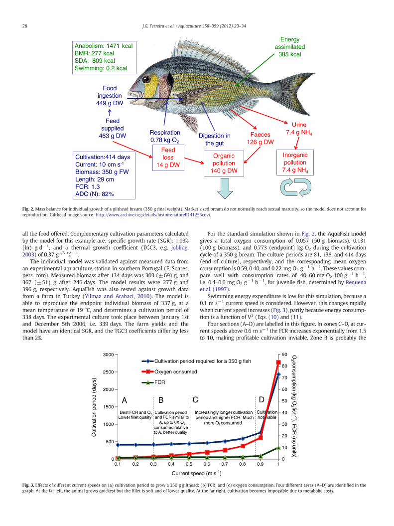
Fig. 3. Effects of different current speeds on (a) cultivation period to grow a 350 g gilthead;graph. At the far left, the animal grows quickest but the fillet is soft and of lower quality. A

For the standard simulation shown in Fig. 2, the AquaFish modelgives a total oxygen consumption of 0.057 (50 g biomass), 0.131(100 g biomass), and 0.773 (endpoint) kg O2 during the cultivationcycle of a 350 g bream. The culture periods are 81, 138, and 414 days(end of culture), respectively, and the corresponding mean oxygenconsumption is 0.59, 0.40, and 0.22 mg O2 g−1 h−1. These values com-pare well with consumption rates of 40–60 mg O2 100 g−1 h−1,i.e. 0.4–0.6 mg O2 g−1 h−1, for juvenile fish, determined by Requenaet al. (1997).

Swimming energy expenditure is low for this simulation, because a0.1 m s−1 current speed is considered. However, this changes rapidlywhen current speed increases (Fig. 3), partly because energy consump-tion is a function of V3 (Eqs. (10) and (11).

Four sections (A–D) are labelled in this figure. In zones C–D, at cur-rent speeds above 0.6 m s−1 the FCR increases exponentially from 1.5to 10, making profitable cultivation inviable. Zone B is probably the

0

10

20

30

40

50

60

70

80

90

0.6 0.7 0.8 0.9 1

quired for a 350 g fish

ed (m s-1)

creasingly longer cultivation eriod and higher FCR. Much

more O2consumed

Cultivation not viable

D

O2 consum

ption (kg O2 fish

-1), FC

R (no units)

(b) FCR; and (c) oxygen consumption. Four different areas (A–D) are identified in thet the far right, cultivation becomes impossible due to metabolic costs.

29J.G. Ferreira et al. / Aquaculture 358–359 (2012) 23–34

most desirable section, where both the cultivation period and FCR areat acceptable levels. Energy costs for aeration will be higher (up to6× more oxygen is consumed) but the fillet quality will improve. Atpresent there is no price differential for aquaculture products, excepton criteria such as organic farming. That in itself is somewhat of aparadox, since the use of species such as the Peruvian anchoveta forfishmeal is simultaneously organic and environmentally unfriendly.

In most markets, there is a discrete and substantial price differencebetween cultivated and wild fish of the same species, with no interme-diate grading based on the quality differential among culture sites. Notonly should a premium be placed on the environmental sustainabilityof the product, but the higher costs associated with better fillets shouldbe compensated by higher prices. This type of gradient is common inother food products, e.g. with cage, cage-free, and free-range eggs.

3.2. IMTA in finfish ponds

The consequences of monoculture versus IMTA are readily observedin onshore aquaculture, which in turn corresponds to a very significantproportion of world aquaculture, due to the role of SE Asia and China inglobal production (FAO, 2011). Before the advent of electrical aerationdevices, pond culture relied on the natural oxygen balance in the cul-ture environment; filter-feeders played a role in removing excess or-ganic material, and autotrophs in removing mineral nutrients andreoxygenating the water. Given the prevalence of pond culture inAsia, perhaps that is one of the historical reasons for IMTA, alongwith the economic advantages of recycling. The key physical and bio-geochemical processes that occur in pond culture were simulatedwith the FARM model, and results are shown for both monoculture ofgilthead and co-cultivation with Pacific oysters (Table 2).

The table shows the model outputs in three blocks, following thePeople–Planet–Profit approach. A relatively low cultivation density

Table 2Key data for gilthead monoculture and IMTA (with bivalves) in onshore ponds, simulated w

Parameter Finfish monoculture

Model setupCultivation practice 1 ha pond, 2 m depth; fish density: 3 ind.m−2 (30,000 fi

culture period, 10% mortality over cycle; water renewal:volume per day, aerators switch on when % saturation D.

Production outputsTotal feed supplied 15,103 kg dry feed pelletsMax individual weight (g) 370Total production (TPP, kg FW) 6272APPa 41.8FCR 2.4

Environmental impactOrganic deposits (kg DW) 11,960Nitrogen regeneration (kg N) 655Primary production (kg N) 251Sediment accretion (mm) 1ASSETS eutrophication

ChlorophyllDissolved oxygenASSETS scoreb

ExternalitiesNH4

+ discharge (kg N) 268Algae (kg chlorophyll) 7.40

Financial dataRevenue (USD) 15,680Costs (all in USD) 11,448

Feed 3927Seed 5265Energy (aeration) 2257

Profit (USD) 4232

a APP: average physical product=total production/total fry or seed biomass, a measureb ASSETS score colours: blue (better), green, yellow, orange, and red (worse).

was used, both for finfish and shellfish, but in a confined environmentthis is sufficient to quantify substantial benefits when gilthead arecultivated in IMTA. From the production side, the feed required bythe finfish is not reduced by IMTA, but if macrobenthic productionwere included in the model, less feed would be required. In IMTA,640 kg of market-size oysters are grown in the 420 day cultivationperiod, providing both goods and services to the farmer. A comple-mentary simulation of oyster monoculture in the same pond (notshown in the table) yields only 1.7 kg of harvestable (60–70 g TFW)oysters for an identical culture period, because the food supply is in-sufficient to grow market-sized shellfish. A reduction in the thresholdharvest weight to 40–50 g TFW yields only 25 kg, i.e. the oysters per-form a bioremediation role but the farmer does not get a crop withinthat cultivation period.

The environmental impact of gilthead culture is substantiallyreduced in IMTA, for an identical finfish yield. The organic depositionto the bottom of the pond is approximately halved, due to bivalvefiltration of POM. The organic material filtered by the oysters is partlydetritus from the finfish culture, and partly primary production dueto nutrient regeneration. The reduction in organic deposits leads toan equivalent 50% reduction in mineral nitrogen released from thesediment; that reduction, coupled with top-down control of phyto-plankton by bivalves, means that net primary production (NPP) inthe pond is reduced in IMTA to 20% of the 251 kg N cycle−1 simulatedfor monoculture.

Other environmental benefits are a 50% reduction in overall accretionof sediments at the bottom of the pond, and a substantial improvementin the ASSETS eutrophication index (Bricker et al., 2003), mainly due tothe reduction in chlorophyll (chl) concentration. If an aquaculturepond is renewing water, then the discharge puts pressure on the receiv-ing body, since the nutrients and algae released have an impact on theenvironment, the cost of which is not internalised by the farmer. A part

ith the FARM model (all results for a complete production cycle).

Finfish+shellfish IMTA (all finfish data unchanged)

sh), 420 day3% pondO. falls below 40%

Pacific oysters added at a density of 5 ind m−2 (50,000 oysters),10% mortality over cycle, 60–70 g harvest weight (total freshweight, TFW)

Feed on organic material in pond370 (finfish)+66 (oysters)6272+639=691141.8+6.4–

5478315530.5

4071.06

15,680+3196=18,87611,448+123=11,57139275265+100=53652257+23=22804232+3073=7305

of return on investment (ROI).

30 J.G. Ferreira et al. / Aquaculture 358–359 (2012) 23–34

of the price differential between SE Asia and western aquaculture is dueto labour costs. Moreover, the lower environmental standards and/orenforcement also increase competitiveness.

The FARMmodel calculates a substantial difference in environmen-tal externalities between gilthead monoculture and IMTA. The massbalance at the end of the culture (Table 2) shows that the ammoniadischarge increases by 52% in IMTA, due to the addition of dissolvednutrients from shellfish excretion, but the particulate waste (whetheraccounted for as chlorophyll or particulate nitrogen) for IMTA is only14% of the discharge when compared to gilthead monoculture. The re-duction in negative externalities due to the co-cultivation of shellfishcorresponds to a waste removal of 9 population-equivalents (PEQ), asubstitution cost of 354 USD y−1. The addition of seaweeds to theIMTA system would recapture inorganic nutrients, further reducingthe environmental impact of combined culture, and potentially provid-ing an extra crop.

In addition to the ecosystem services provided by IMTA, the overall(goods) revenue increases by 20%, from about 15.5 kUSD to 19 kUSD.However, the profit increase is much more striking, since a large partof the revenue from gilthead culture is spent on feed and energy.Profits rise from 4232 USD per cycle to 7305 USD, i.e. a 70% increase.

3.3. Offshore aquaculture

3.3.1. IMTA in offshore sitesThe results for the standard offshore culture model are shown in

Table 3, for monoculture of finfish and shellfish, and the two combinedin IMTA. There are several important differences when compared topond culture, due to the dilution effect of offshore waters. Concentra-tions of nutrients and chlorophyll are much lower in the offshorecase, even for finfish monoculture. Contrary to the pond simulations,FARM is not using diagenesis to reintroduce recycled materials into

Table 3Simulation results for gilthead and Pacific oysters in offshore culture using the FARM mode

Parameter Finfish monoculturea

Production outputsTotal feed supplied 2204 t dry feed pelletsTotal production (TPP, tonnes FW) 997APP 26.6FCR 2.2

Environmental impactOrganic deposits (ton POC y−1)d 131.9Organic deposits (kg POC m−2 y−1) 0.88ASSETS eutrophication

ChlorophyllDissolved oxygenASSETS scoree

Positive externalities –

Population equivalents (PEQ) –

Nutrient credits (kUSD) –

Financial dataRevenue (all kUSD) 2494

Farmgate value 2494Ecosystem services –

Costs (all in kUSD) 1889Feed 573Seed 1316

Profit (kUSD) 604

a 200 m (wide)×750 m (long) farm, 10 m depth, 5 sections (each 150 m long); finfishcurrent speed: bidirectional flow over a semi-diurnal cycle, peak spring tide: 0.2 m s−1, an

b Pacific oysters at a density of 100 ind.m−2 (15×106 oysters), 10% mortality over cyclec Combination of finfish and shellfish as per the data in the above notes. Financial data c

because shellfish production is enhanced in IMTA.d Due to cultivation only. Natural sedimentation of particles without any cultivation is dee ASSETS score colours: blue (better), green, yellow, orange, and red (worse).

the offshore farm area, because (i) processing of organic matter inthe sediment does not feed back to the farm; and (ii) mixing dilutesthe waste products of gilthead culture, even at the relatively high den-sities of 50 ind.m−2. The percentile 90 (P90) for NH4

+ over the 420 dayculture cycle is about 10 μmol L−1, an order of magnitude lower thanthe value of 192 μmol L−1 obtained in IMTA pond culture.

There are no dissolved oxygen problems, and therefore no needfor aerators, in either of the three (two monoculture and one IMTA)scenarios. Low values were used for environmental drivers of shell-fish growth, since these are typical of offshore areas. The meanvalue for chlorophyll a outside the farm was 0.6 μg L−1 (C.V. 24%),with similarly low POM (3.2 mg L−1, C.V. 28%, POM/TPM: 0.19).Values of this order are typical of offshore waters, and the combina-tion of finfish and shellfish culture enhances bivalve production byproviding additional organic detritus as a food supplement. Over theentire cycle, IMTA provides a 20% increase in oyster production,corresponding to an additional 41 tTFW of harvestable biomass.

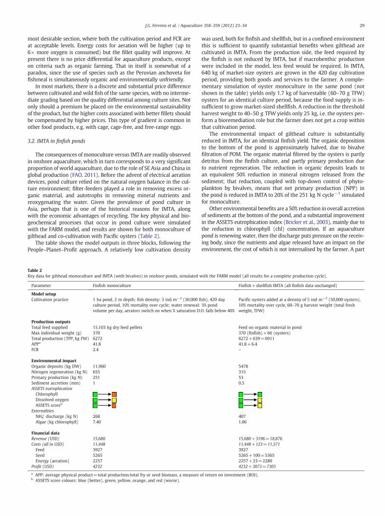
In parallel, the oysters provide a substantial ecosystem benefit byremoving a (net) population-equivalent (PEQ) loading equal to 5500people. The organic deposition is reduced by about 7% in IMTA,although the shellfish also add particulate waste to the culture areadue to faeces and pseudofaeces. A full mass balance for the cultivationof shellfish in IMTA is shown in Fig. 4.

The main difference between the mass balance for shellfish mono-culture and that shown in Fig. 4 is the removal of organic detritus.Whereas the phytoplankton removed is only 0.5% higher than inmonoculture, the removal of detritus increases by 3%. If the concentra-tion of phytoplankton (chl) is increased in the water outside the farm,the differences in shellfish yield from monoculture to IMTA becomenegligible. This is to be expected given the higher energy content ofalgae (Platt and Irwin, 1973), and selection for phytoplankton infilter-feeding bivalves (Cranford et al., 2011).

l (all results for a complete production cycle).

Shellfish monocultureb Finfish+shellfish IMTAc

Natural organics Organics202.9 997+243.7=1240.76.8 26.6+8.1– –

103.7 122.10.69 0.81

4692 4830188 193

1203 2494+1412=39061015 2494+1219=3713188 19330 1889+30=1919– 57330 1316+30=13461173 604+1382=1986

density: 50 ind.m−2 (7.5×106 fish), 420 day culture period, 10% mortality over cycle;d peak neap tide: 0.1 m s−1., 90 g harvest weight (TFW). All physical parameters as for finfish.ombines finfish and shellfish, but shellfish data are better than for oyster monoculture

termined by the model as 722 tPOC y−1, a background accretion rate of 4.9 mm y−1.

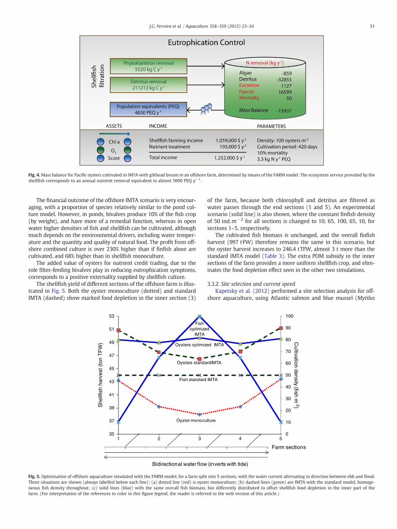
Fig. 4.Mass balance for Pacific oysters cultivated in IMTA with gilthead bream in an offshore farm, determined by means of the FARMmodel. The ecosystem service provided by theshellfish corresponds to an annual nutrient removal equivalent to almost 5000 PEQ y−1.

31J.G. Ferreira et al. / Aquaculture 358–359 (2012) 23–34

The financial outcome of the offshore IMTA scenario is very encour-aging, with a proportion of species relatively similar to the pond cul-ture model. However, in ponds, bivalves produce 10% of the fish crop(by weight), and have more of a remedial function, whereas in openwater higher densities of fish and shellfish can be cultivated, althoughmuch depends on the environmental drivers, including water temper-ature and the quantity and quality of natural food. The profit from off-shore combined culture is over 230% higher than if finfish alone arecultivated, and 68% higher than in shellfish monoculture.

The added value of oysters for nutrient credit trading, due to therole filter-feeding bivalves play in reducing eutrophication symptoms,corresponds to a positive externality supplied by shellfish culture.

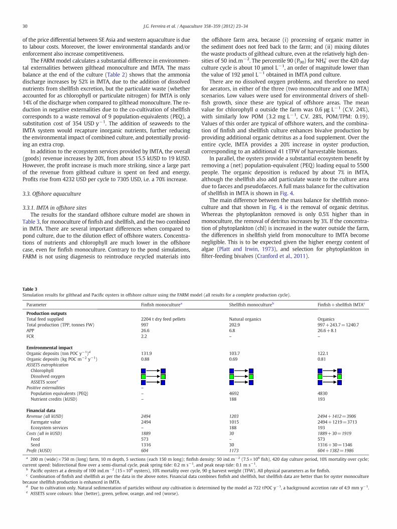
The shellfish yield of different sections of the offshore farm is illus-trated in Fig. 5. Both the oyster monoculture (dotted) and standardIMTA (dashed) show marked food depletion in the inner section (3)

35

37

39

41

43

45

47

49

51

53

1 2 3

Oyster monocu

She

llfis

h ha

rves

t (to

n T

FW

)

Fish optimize

IMTA

Fish standard

Oysters optimiz

Oysters standa

Bidirectional water flow

Fig. 5. Optimisation of offshore aquaculture simulated with the FARM model, for a farm splitThree situations are shown (always labelled below each line): (a) dotted line (red) is oysteneous fish density throughout; (c) solid lines (blue) with the same overall fish biomass,farm. (For interpretation of the references to color in this figure legend, the reader is referr

of the farm, because both chlorophyll and detritus are filtered aswater passes through the end sections (1 and 5). An experimentalscenario (solid line) is also shown, where the constant finfish densityof 50 ind.m−2 for all sections is changed to 10, 65, 100, 65, 10, forsections 1–5, respectively.

The cultivated fish biomass is unchanged, and the overall finfishharvest (997 tFW) therefore remains the same in this scenario, butthe oyster harvest increases to 246.4 tTFW, almost 3 t more than thestandard IMTA model (Table 3). The extra POM subsidy in the innersections of the farm provides a more uniform shellfish crop, and elim-inates the food depletion effect seen in the other two simulations.

3.3.2. Site selection and current speedKapetsky et al. (2012) performed a site selection analysis for off-

shore aquaculture, using Atlantic salmon and blue mussel (Mytilus

0

10

20

30

40

50

60

70

80

90

100

4 5

lture

Farm sections

Cu

ltivation density (fish m

-2)

d

IMTA

ed IMTA

rdIMTA

(inverts with tide)

into 5 sections, with the water current alternating in direction between ebb and flood.r monoculture; (b) dashed lines (green) are IMTA with the standard model, homoge-but differently distributed to offset shellfish food depletion in the inner part of theed to the web version of this article.)

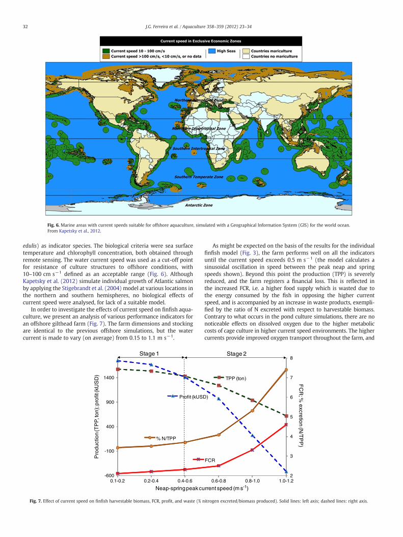
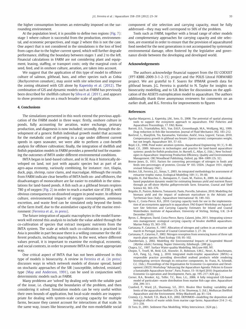
Fig. 6. Marine areas with current speeds suitable for offshore aquaculture, simulated with a Geographical Information System (GIS) for the world ocean.From Kapetsky et al., 2012.

32 J.G. Ferreira et al. / Aquaculture 358–359 (2012) 23–34

edulis) as indicator species. The biological criteria were sea surfacetemperature and chlorophyll concentration, both obtained throughremote sensing. The water current speed was used as a cut-off pointfor resistance of culture structures to offshore conditions, with10–100 cm s−1 defined as an acceptable range (Fig. 6). AlthoughKapetsky et al. (2012) simulate individual growth of Atlantic salmonby applying the Stigebrandt et al. (2004) model at various locations inthe northern and southern hemispheres, no biological effects ofcurrent speed were analysed, for lack of a suitable model.

In order to investigate the effects of current speed on finfish aqua-culture, we present an analysis of various performance indicators foran offshore gilthead farm (Fig. 7). The farm dimensions and stockingare identical to the previous offshore simulations, but the watercurrent is made to vary (on average) from 0.15 to 1.1 m s−1.

-600

-100

400

900

1400

Profit (kUS

% N/TPP

Neap-spring peak cu

Pro

duct

ion

(TP

P, t

on);

pro

fit (k

US

D)

0.1-0.2 0.2-0.4 0.4-0.6

Stage 1

Fig. 7. Effect of current speed on finfish harvestable biomass, FCR, profit, and waste (% n

As might be expected on the basis of the results for the individualfinfish model (Fig. 3), the farm performs well on all the indicatorsuntil the current speed exceeds 0.5 m s−1 (the model calculates asinusoidal oscillation in speed between the peak neap and springspeeds shown). Beyond this point the production (TPP) is severelyreduced, and the farm registers a financial loss. This is reflected inthe increased FCR, i.e. a higher food supply which is wasted due tothe energy consumed by the fish in opposing the higher currentspeed, and is accompanied by an increase in waste products, exempli-fied by the ratio of N excreted with respect to harvestable biomass.Contrary to what occurs in the pond culture simulations, there are nonoticeable effects on dissolved oxygen due to the higher metaboliccosts of cage culture in higher current speed environments. The highercurrents provide improved oxygen transport throughout the farm, and

2

3

4

5

6

7

8

TPP (ton)

D)

FCR

rrent speed (m s-1)

FC

R; %

excretion (N/T

PP

)

0.6-0.8 0.8-1.0 1.0-1.2

Stage 2

itrogen excreted/biomass produced). Solid lines: left axis; dashed lines: right axis.

33J.G. Ferreira et al. / Aquaculture 358–359 (2012) 23–34

the higher consumption becomes an externality imposed on the sur-rounding environment.

At the population level, it is possible to define two regions (Fig. 7):stage 1 where culture is successful from the production, environmen-tal, and economic perspectives, and stage 2 where this is not the case.One aspect that is not considered in the simulations is the loss of feedfrom cages due to the higher current speed, which will further degradeperformance, shifting the boundary between stages 1 and 2 to the left.Financial calculations in FARM are not considering plant and equip-ment, leasing, staffing, or transport costs; only the marginal costs ofseed, feed, and in onshore culture, aeration, are taken into account.

We suggest that the application of this type of model to offshoreculture of salmon, gilthead, bass, and other species such as Cobia(Rachycentron canadum), may assist with site selection and improvethe zoning obtained with GIS alone by Kapetsky et al. (2012). Thecombination of GIS and dynamic models such as FARM has previouslybeen described for shellfish culture by Silva et al. (2011), and appearsto show promise also on a much broader scale of application.

4. Conclusions

The simulations presented in this work extend the previous appli-cation of the FARM model in three ways: firstly, onshore culture inponds, fully accounting for aeration, water exchange, primaryproduction, and diagenesis is now included; secondly, through the de-velopment of a generic finfish individual growth model that accountsfor the metabolic cost of growing in a cage under different currentspeeds in open seawater, we were able to perform a cost–benefitanalysis for offshore cultivation; finally, the integration of shellfish andfinfish population models in FARM provides a powerful tool for examin-ing the outcomes of IMTA under different environmental conditions.

IMTA began in land-based culture, and in SE Asia it historically de-veloped on land, not just with aquatic species but as part of anagro-aqua economy, variously combining, for instance: rice, tilapia,duck, pigs, shrimp, razor clams, and macroalgae. Although the resultsfrom FARM indicate clear benefits of IMTA both on- and offshores, thedisadvantages of monoculture are far easier to establish in the simu-lations for land-based ponds. A fish such as a gilthead bream respires780 g of oxygen (Fig. 2) in order to reach a market size of 350 g, withobvious consequences on dissolved oxygen in pond water. In offshoreculture, environmental impacts of oxygen consumption, ammoniaexcretion, and waste feed can be simulated only beyond the limitsof the farm itself, due to the assimilative capacity of the marine envi-ronment (Ferreira et al., in press).

The future integration of aquatic macrophytes in the model frame-work will extend this analysis to include the value added through theco-cultivation of species that extract inorganic nutrients from theIMTA system. The scale at which such co-cultivation is practised inAsia is possible in part because there is a willing consumer for the dif-ferent products, including macrophytes. In the west, where differentvalues prevail, it is important to examine the ecological, economic,and social contexts, in order to promote IMTA in the most appropriateway.

One critical aspect of IMTA that has not been addressed in thistype of models is biosecurity. A review in Ferreira et al. (in press)discusses ways in which network models of disease spread, basedon stochastic approaches of the SIR (susceptible, infected, resistant)type (May and Anderson, 1991), can be used in conjunction withdeterministic models such as FARM.

Many problems are ‘solved’ by dealing only with the soluble partof the issue, i.e. changing the boundaries of the problem, and thenconsidering it solved. Simulation models can be very useful withintheir own bounds of application, but local-scale models are inappro-priate for dealing with system-scale carrying capacity for multiplefarms, because they cannot account for interactions at that scale. Inthe same way, issues like biosecurity, and the non-modellable social

component of site selection and carrying capacity, must be fullyaddressed―they may well correspond to 50% of the problem.

Tools such as FARM, together with a broad range of other modelsand complementary approaches for carrying capacity and site selec-tion, are essential in order to ensure that the provision of aquaculturedfood needed for the next generations is not accompanied by systematicenvironmental damage, often fostered by the legislative and gover-nance divide between the developing and developed world.

Acknowledgements

The authors acknowledge financial support from the EU COEXIST(FP7-KBBE-2009-3-1-2-15) project and the POLIS Litoral FORWARDproject. We are grateful to F. Soares for IPIMAR growth data forgilthead bream. J.G. Ferreira is grateful to N. Taylor for insights onbiosecurity modelling, and to S.B. Bricker for discussions on the appli-cation of the ASSETS eutrophication model to aquaculture. The authorsadditionally thank three anonymous reviewers for comments on anearlier draft, and R.G. Ferreira for improvements to figures

References

Aguilar-Manjarrez, J., Kapetsky, J.M., Soto, D., 2008. The potential of spatial planningtools to support the ecosystem approach to aquaculture. FAO Fisheries andAquaculture Proceedings, 17. FAO, Rome.

Barrett, D.S., Triantafyllou, M.S., Yue, D.K.P., Grosenbaugh, M.A., Wolfgang, M.J., 1999.Drag reduction in fish-like locomotion. Journal of Fluid Mechanics 392, 183–212.

Bavčević, L., Klanjšček, Tin, Karamarko, Vatroslav, Aničić, Ivica, Legović, Tarzan, 2010.Compensatory growth in gilthead sea bream (Sparus aurata) compensates weight,but not length. Aquaculture 301, 57–63.

Boyd, C.E., 1998. Pond water aeration systems. Aquacultural Engineering 18 (1), 9–40.Boyd, C.E., 2009. Advances in technologies and practice for land-based aquaculture

systems: ponds for finfish production. In: Burnell, G., Allan, G. (Eds.), New Technol-ogies in Aquaculture: Improving Production Efficiency, Quality and EnvironmentalManagement. CRC/Woodhead Publishing, Oxford, pp. 984–1009 (Ch. 32).

Breese Jones, D., 1931. Factors for converting percentages of nitrogen in foods andfeeds into percentages of proteins. Circular Nº 183. USDA. (August 1931, slightlyrevised February 1941).

Bricker, S.B., Ferreira, J.G., Simas, T., 2003. An integrated methodology for assessment ofestuarine trophic status. Ecological Modelling 169 (1), 39–60.

Brigolin, D., Dal Maschio, G., Ramapazzo, F., Giani, M., Pastres, R., 2009. An individual-based population dynamic model for estimating biomass yield and nutrient fluxesthrough an off-shore Mytilus galloprovincialis farm. Estuarine, Coastal and ShelfScience 82, 365–376.

Brigolin, D., Pastres, Roberto, Tomassetti, Paolo, Porrello, Salvatore, 2010. Modelling thebiomass yield and the impact of seabream mariculture in the Adriatic andTyrrhenian Seas (Italy). Aquaculture International 18, 149–163.

Byron, C., Costa-Pierce, B.A., 2010. Carrying capacity tools for use in the implementa-tion of an ecosystems approach to aquaculture. FAO Expert Workshop on Aquacul-ture Site Selection and Carrying Capacity Estimates for Inland and CoastalWaterbodies. Institute of Aquaculture, University of Stirling, Stirling, U.K. (6–8December 2010).

Byron, C., Bengtson, David, Costa-Pierce, Barry, Calanni, John, 2011. Integrating scienceinto management: ecological carrying capacity of bivalve shellfish aquaculture.Marine Policy 35, 363–370.

Cartaxana, P., Catarino, F., 1997. Allocation of nitrogen and carbon in an estuarine saltmarsh in Portugal. Journal of Coastal Conservation 3, 27–34.

Cartaxana, P., Catarino, F., 2002. Nitrogen resorption from senescing leaves of three saltmarsh plant species. Plant Ecology 159, 95–102.

Chamberlain, J., 2002. Modelling the Environmental Impacts of Suspended Mussel(Mytilus edulis) Farming. Napier University, Edinburgh. (200 pp.).

Chapra, S.C., 1997. Surface Water-quality Modelling. McGraw-Hill, NY.Chopin, T., Troell, M., Reid, G.K., Knowler, D., Robinson, S.M.C., Neori, A., Buschmann,

A.H., Pang, S.J., Fang, J., 2010. Integrated multi-trophic aquaculture (IMTA)—aresponsible practice providing diversified seafood products while renderingbiomitigating services through its extractive components. In: Franz, N., Schmidt,C.C. (Eds.), Proceedings of the Organisation for Economic Co-operation and Devel-opment (OECD) Workshop “Advancing the Aquaculture Agenda: Policies to Ensurea Sustainable Aquaculture Sector”, Paris, France, 15–16 April 2010. Organisation forEconomic Co-operation and Development, Paris, pp. 195–217 (426 pp.).

Corner, R.A., Brooker, A.J., Telfer, T.C., Ross, L.G., 2006. A fully integrated GIS-basedmodel of particulate—waste distribution from marine fish-cage sites. Aquaculture258, 299–311.

Cranford, P., Ward, J.E., Shumway, S.E., 2011. Bivalve filter feeding: variability andlimits of the aquaculture biofilter (Ch. 4) In: Shumway, S. (Ed.), Molluscan ShellfishAquaculture and the Environment. Wiley-Blackwell, pp. 81–124.

Cromey, C.J., Nickell, T.D., Black, K.D., 2002. DEPOMOD—modelling the deposition andbiological effects of waste solids from marine cage farms. Aquaculture 214 (1–4),211–239.

Di Toro, D., 2001. Sediment Flux Modelling. Wiley Interscience. (624 pp.).

34 J.G. Ferreira et al. / Aquaculture 358–359 (2012) 23–34

Elliott, J.M., Davidson, W., 1975. Energy equivalents of oxygen consumption in animalenergetics. Oecologia 19, 195–201.

Elliott, J.M., Persson, L., 1978. The estimation of daily rates of food consumption for fish.The Journal of Animal Ecology 47 (3), 977–991.

European Commission Fisheries, 2011. Marine species (farmed fish and shellfish)Available:http://ec.europa.eu/fisheries/marine_species/index_en.htm.

FEAP—Federation of European Aquaculture Producers, 2009. Production and PriceReports of Member Associations of the F.E.A.P. 2001–2008. FEAP Secretariat,Liége, Belgium. ( http://www.aquamedia.org).

Ferreira, J.G., Hawkins, A.J.S., Bricker, S.B., 2007. Management of productivity, environ-mental effects and profitability of shellfish aquaculture—the farm aquacultureresource management (FARM) model. Aquaculture 264, 160–174.

Ferreira, J.G., Anderson, H.C., Corner, R.A., Desmit, X., Fang, Q., de Goede, E.D., Groom,S.B., Gu, H., Gustafsson, B.G., Hawkins, A.J.S., Hutson, R., Jiao, H., Lan, D., Lencart-Silva, J., Li, R., Liu, X., Luo, Q., Musango, J.K., Nobre, A.M., Nunes, J.P., Pascoe, P.L.,Smits, J.G.C., Stigebrandt, A., Telfer, T.C., de Wit, M.P., Yan, X., Zhang, X.L., Zhu,M.Y., Zhu, C.B., Bricker, S.B., Xiao, Y., Xu, S., Nauen, C.E., Scalet, M., 2008a. Sustain-able options for people, catchment and aquatic resources. In: InternationalCollaboration on Integrated Coastal Zone Management (Ed.), The SPEAR Project.IMAR—Institute of Marine Research/European Commission (180 pp. Available:http://www.biaoqiang.org/documents/SPEAR/book.pdf).

Ferreira, J.G., Hawkins, A.J.S., Monteiro, P., Moore, H., Service, M., Pascoe, P.L., Ramos, L.,Sequeira, A., 2008b. Integrated assessment of ecosystem-scale carrying capacity inshellfish growing areas. Aquaculture 275, 138–151.

Ferreira, J.G., Sequeira, A., Hawkins, A.J.S., Newton, A., Nickell, T., Pastres, R., Forte, J.,Bodoy, A., Bricker, S.B., 2009. Analysis of coastal and offshore aquaculture: applicationof the FARM model to multiple systems and shellfish species. Aquaculture 289,32–41.

Ferreira, J.G., Aguilar-Manjarrez, J., Bacher, C., Black, K., Dong, S.L., Grant, J., Hofmann, E.,Kapetsky, J., Leung, P.S., Pastres, R., Strand, Ø., Zhu, C.B., 2010. Expert panel presenta-tion V.3. Progressing aquaculture through virtual technology and decision-makingtools for novel management. Book of Abstracts, Global Conference on Aquaculture2010, 22–25 September 2010. FAO/NACA/Thailand Department of Fisheries,Bangkok, Thailand, pp. 91–93.

Ferreira, J.G., Hawkins, A.J.S., Bricker, S.B., 2011. The role of shellfish farms in provisionof ecosystem goods and services (Ch. 1) In: Shumway, S. (Ed.), Molluscan ShellfishAquaculture and the Environment. Wiley-Blackwell, pp. 3–31.

Ferreira, J.G., Grant, J., Verner-Jeffreys, D., Taylor, N., in press. Modeling frameworks fordetermination of carrying capacity for aquaculture, in: Meyers, Robert A. (Ed.),Encyclopedia of Sustainability Science and Technology. Springer (ISBN: 978-0387894690).

Food andAgriculture Organization of theUnitedNations, 2011. CulturedAquaculture Spe-cies Information Programme. http://www.fao.org/fishery/culturedspecies/search/en.

Franco, A.R., Ferreira, J.G., Nobre, A.M., 2006. Development of a growth model forpenaeid shrimp. Aquaculture 259, 268–277.

Giles, H., Broekhuizen, N., Bryan, K.R., Pilditch, C.A., 2009. Modelling the dispersal ofbiodeposits from mussel farms: the importance of simulating biodeposit erosionand decay. Aquaculture 291, 168–178.

Gosch, N.J.C., Pope, Kevin L., Michaletz, Paul H., 2009. Stomach capacities of six fresh-water fishes. Journal of Freshwater Ecology 24 (4), 645–649.

Gray, J., 1936. Studies in animal locomotion VI: the propulsive powers of the dolphin.The Journal of Experimental Biology 13, 192–199.

Gray, I.E., 1953. The relation of body weight to body surface area in marine fishes. TheBiological Bulletin 105, 285–288.

Grigorakis, K., 2007. Compositional and organoleptic quality of farmed and wildgilthead sea bream (Sparus aurata) and sea bass (Dicentrarchus labrax) and factorsaffecting it: a review. Aquaculture 272, 55–75.

Gul, Y., Salim, M., Rabbani, B., 2007. Evaluation of apparent digestibility coefficients ofdifferent dietary protein levels with and without fish meal for Labeo rohita.Pakistan Veterinary Journal 27 (3), 121–125.

Hernández, J.M., Gasca-Leyva, Eucario, León, Carmelo J., Vergara, J.M., 2003. A growthmodel for gilthead seabream (Sparus aurata). Ecological Modelling 165, 265–283.

Holmer, M., 2010. Environmental issues of fish farming in offshore waters: perspec-tives, concerns and research needs. Aquaculture Environment Interactions 1,57–70.

Jobling, M., 1981. Mathematical models of gastric emptying and the estimation of dailyrates of food consumption for fish. Journal of Fish Biology 19, 245–257.

Jobling, M., 2003. The thermal growth coefficient (TGC) model of fish growth: acautionary note. Aquaculture Research 34 (7), 581–584.

Kapetsky, J.M., Aguilar-Manjarrez, J., Jenness, J., 2012. A spatial assessment of potentialfor offshore mariculture development from a global perspective. FAO Fisheries andAquaculture Technical Paper. No. 549. FAO, Rome.

Knight, R.L., Margraf, F. Joseph, 1982. Estimating stomach fullness in fishes. NorthAmerican Journal of Fisheries Management 2 (4), 413–414.

Libralato, S., Solidoro, C., 2008. A bioenergetic growth model for comparing Sparusaurata's feeding experiments. Ecological Modelling 214, 325–337.

May, R.L., Anderson, R.M., 1991. Infectious Diseases of Humans: Dynamics and Control.Oxford University Press, Oxford, U.K.0-19-854040-X.

Moo, T.S.Y., undated. Excerpts from Chinese fish culture, by Fan Lee. Contribution No.459, Chesapeake Biological Laboratory. University of Maryland, Solomons,Maryland, U.S.A.

National Research Council—NRC, 1993. Nutrient Requirements of Fish. National Academyof Science of Washington, Washington, USA.

Neori, A., Chopin, T., Troell, M., Buschmann, A.H., Kraemer, G.P., Halling, C., Shpigel, M.,Yarish, C., 2004. Integrated aquaculture: rationale, evolution and state of the artemphasizing seaweed biofiltration in modern mariculture. Aquaculture 231(1–4), 361–391.

Niimi, A.J., 1975. Relationship of body surface-area to weight in fishes. Canadian Journalof Zoology 53 (8), 1192–1194.

Nobre, A.M., Ferreira, J.G., Newton, A., Simas, T., Icely, J.D., Neves, R., 2005. Managementof coastal eutrophication: integration of field data, ecosystem-scale simulationsand screening models. Journal of Marine Systems 56, 375–390.

Nobre, A.M., Ferreira, J.G., Nunes, J.P., Yan, X., Bricker, S., Corner, R., Groom, S., Gu, H.,Hawkins, A.J.S., Hutson, R., Lan, D., Lencart e Silva, J.D., Pascoe, P., Telfer, T.,Zhang, X., Zhu, M., 2010. Assessment of coastal management options by means ofmultilayered ecosystem models. Estuarine, Coastal and Shelf Science 87, 43–62.

Nunes, J.P., Ferreira, J.G., Bricker, S.B., O'Loan, B., Dabrowski, T., Dallaghan, B., Hawkins,A.J.S., O'Connor, B., O'Carroll, T., 2011. Towards an ecosystem approach toaquaculture: assessment of sustainable shellfish cultivation at different scales ofspace, time and complexity. Aquaculture 315, 369–383.

Olesen, I., Myhr, A.I., Rosendal, G.K., 2010. Sustainable aquaculture: are we gettingthere? Ethical perspectives on salmon farming. Journal of Agricultural andEnvironmental Ethics 24, 381–408.

Oliveira, A.C.B., Martinelli, L.A., Moreira, M.Z., Cyrino, J.E.P., 2008. Determination ofapparent digestibility coefficient in fish by stable carbon isotopes. AquacultureNutrition 14, 10–13.

Palma, J., Andrade, J.P., Paspatis, M., Divanach, P., Kentouri, M., 1998. Morphometriccharacters in gilthead sea bream, Sparus aurata, red porgy, Pagrus pagrus andtheir hybrids (Sparidae). Italian Journal of Zoology 65, 435–439.

Piedecausa, M.A., Aguado-Giménez, F., Cerezo-Valverde, J., Hernández-Llorente, M.D.,García-García, B., 2010. Simulating the temporal pattern of waste production infarmed gilthead seabream (Sparus aurata), European seabass (Dicentrarchuslabrax) and Atlantic bluefin tuna (Thunnus thynnus). Ecological Modelling 221,634–640.

Platt, T., Irwin, B., 1973. Caloric content of phytoplankton. Limnology and Oceanography18 (2), 306–310.

Requena, A., Fernández-Borrás, J., Planas, J., 1997. The effects of a temperature rise onoxygen consumption and energy budget in gilthead sea bream. AquacultureInternational 5, 415–426.

Silva, C., Ferreira, J.G., Bricker, S.B., DelValls, T.A., Martín-Díaz, M.L., Yañez, E., 2011. Siteselection for shellfish aquaculture by means of GIS and farm-scale models, with anemphasis on data-poor environments. Aquaculture 318, 444–457.

Simas, T.C., Ferreira, J.G., 2007. Nutrient enrichment and the role of salt marshes in theTagus estuary (Portugal). Estuarine, Coastal and Shelf Science 75, 393–407.

Skogen, M.D., Eknes, M., Asplin, L.C., Sandvik, A.D., 2009. Modelling the environmentaleffects of fish farming in a Norwegian fjord. Aquaculture 298, 70–75.

Steinhausen, M.F., Steffensen, J.F., Andersen, N.G., 2010. The effects of swimmingpattern on the energy use of gilthead seabream (Sparus aurata L.). Marine andFreshwater Behaviour and Physiology 43 (4), 227–241.

Stigebrandt, A., Aure, J., Ervik, A., Hansen, P.K., 2004. Regulating the local environmentalimpact of intensive marine fish farming III. A model for estimation of the holdingcapacity in the modelling–ongrowing fish farm–monitoring system. Aquaculture234, 239–261.

Troell, M., Joyce, Alyssa, Chopin, Thierry, Neori, Amir, Buschmann, Alejandro H., Fang,Jian-Guang, 2009. Ecological engineering in aquaculture—potential for integratedmulti-trophic aquaculture (IMTA) in marine offshore systems. Aquaculture 297(1–4), 1–9.

Tucker, C., 2005. Pond aeration. SRAC Publication No. 3700. Southern RegionalAquaculture Center.

Verbeke,W., Sioen, I., Brunsø, K., De Henauw, S., Van Camp, J., 2007. Consumer perceptionversus scientific evidence of farmed andwild fish: exploratory insights from Belgium.Aquaculture International 15, 121–136.

Vogel, S., 1994. Life in moving fluids, The Physical Biology of Flow2nd edition. PrincetonUniversity Press, N.J. (467 pp.).

Wassef, E.A., Shehata, M.B., 1990. Biochemical composition of gilthead bream Sparusaurata L. from Lake Bardawil (Egypt). JKAU Marine Sciences l, 55–65.

Webb, P.W., 1975. Hydrodynamics and energetics of fish propulsion. Bulletin of theFisheries Research Board of Canada 190, 1–158.

Yilmaz, Y., Arabaci, M., 2010. The influence of stocking density on growth and feedefficiency in gilthead seabream, Sparus aurata. Journal of Animal and VeterinaryAdvances 9 (8), 1280–1284.

Zhang, J., Hansen, P.K., Fang, J., Wang, W., Jiang, Z., 2009. Assessment of the local envi-ronmental impact of intensive marine shellfish and seaweed farming—applicationof the MOM system in the Sungo Bay, China. Aquaculture 287, 304–310.