Generated using version 3.0 of the official AMS LATEX template

Croll Revisited:

Why is the Northern Hemisphere Warmer than

the Southern Hemisphere?

Sarah M. Kang ∗

Department of Applied Physics and Applied Mathematics

Columbia University, New York, New York

Richard Seager

Lamont Doherty Earth Observatory

Columbia University, Palisades, New York

∗Corresponding author address: Sarah M. Kang, S.W. Mudd Room 290, Columbia University, New York,

NY 10027. E-mail: smk2182@columbia.edu

1

ABSTRACT

The question of why, in the annual mean, the Northern Hemisphere is warmer than

the Southern Hemisphere is addressed, revisiting an 1870 paper by James Croll. We first

show that the ocean is warmer than the land in general which, acting alone, would make

the Southern Hemisphere warmer because of its greater fraction of ocean. Croll recognized

this and thought it was caused by greater humidity and greenhouse trapping over the ocean

than over the land. However, for any given temperature, greenhouse trapping is actually

greater over the land than the ocean. Instead, oceans are warmer than land because of

smaller surface albedo. However, inter-hemispheric differences in total albedo are negligible

because the impact of differences in land-sea fraction are offset by Southern Hemisphere

ocean and land reflecting more than their Northern Hemisphere counterparts. In agreement

with Croll, it is shown that northward cross-equatorial ocean heat transport is critical for

the Northern Hemisphere to be warmer. This is examined in a simple box model based on

the energy budget of each hemisphere. This inter-hemispheric difference forced by ocean

heat transport is enhanced by the positive water vapor-greenhouse feedback, and is partly

compensated by the southward atmospheric energy transport, which is accomplished by

locating the Intertropical Convergence Zone in the Northern Hemisphere. However, to fully

explain the temperature difference in this way requires a northward ocean heat transport

at the extreme of observational estimates. A better fit to data is found when a larger

basic state greenhouse trapping in the NH, conceived as imposed by continental geometry,

is also imposed. Therefore, despite some modifications to his theory, analysis of modern

data confirms Croll’s 140 year-old theory that the Northern Hemisphere is warmer than the

Southern Hemisphere in part because of northward cross-equatorial ocean heat transport.

1

1. Introduction

One of the most fundamental features of the Earth’s climate is that the Northern Hemi-

sphere (NH) is warmer than the Southern Hemisphere (SH) (Fig. 1). There are several

possible reasons for this. An informal poll of members of the public and some scientists

often produces the answer that it is because the NH has more land and, therefore, heats

up more in summer because of the lesser heat capacity. On the other hand, many scien-

tists argue that it is because the ocean transports heat northward across the equator. We

have also encountered more subtle arguments such as continental geometry that results in

upwelling and equatorward sea ice export in the Antarctic Circumpolar Current (ACC) and

Southern Ocean (SO) cooling the SH. Also, it could be argued that the impact of conti-

nental geometry on subtropical coastal upwelling preferentially cools the south (Philander

et al. 1996). Finally, it could be a transient response to greenhouse gas forcing because the

NH has the larger land fraction and heats up faster than the more oceanic SH. While the

inter-hemispheric temperature asymmetry is interesting in and of itself, it is also of practical

importance because of the influence it exerts on the position of the Intertropical Convergence

Zone (ITCZ) (Kang et al. 2008) whose rains are relied upon many tropical societies for their

water and food production.

Although it still seems unclear exactly why the NH is warmer than the SH, James Croll,

the founder of the astronomical theory of the ice ages, provided an explanation as early as

1870 (Croll 1870). He thought that the hemisphere with more ocean should be warmer than

the one with more land because of higher atmospheric humidity, and hence, more greenhouse

trapping. Interestingly, we will show that this is in fact incorrect: the greenhouse trapping

2

in general is greater over land than over ocean at the same temperature. Nonetheless, given

that he thought that this mechanism would make the SH warmer than the NH, Croll claimed

that the NH was actually warmer because the ocean transports heat northward across the

equator:

The lower mean temperature of the southern hemisphere is due to the amount of

heat transferred over from that hemisphere to the northern by ocean-currents.

Croll�s arguments for how currents accomplish this transport was stated as follows:

Since there is a constant flow of water from the southern hemisphere to the

northern in the form of surface currents, it must be compensated by undercur-

rents of equal magnitude from the northern hemisphere to the southern. The

currents, however, which cross the equator are far higher in temperature than

their compensating undercurrents; consequently there is constant transference of

heat from the southern hemisphere to the northern.

He argues that this idea is supported by the fact that the tropical oceans are cooler than the

tropical land as a result of the huge ocean heat flux divergence. While Croll was correct that

ocean heat flux divergence does cool some equatorial ocean regions, averaged over longitude

it turns out that the tropical oceans are warmer than the tropical land masses. Nevertheless,

Croll�s northward cross-equatorial ocean heat transport (OHT) explanation is probably the

dominant one amongst scientists (e.g. Toggweiler and Bjornsson 2000). It is truly remarkable

that in 1870, Croll 1) knew that the NH was warmer than the SH, 2) was able to infer a

cross-equatorial OHT and 3) provided a coherent explanation for the temperature asymmetry

3

that, though largely forgotten, is still invoked 140 years later. As we will show here, Croll

appears to have been correct.

2. Data

For temperature, NCEP/NCAR reanalysis data (Kistler and Coauthors 2001) for the

period from 1979 to 2009 are used. The annual mean as well as seasonal averages will be

analyzed where winter (summer) in the NH is computed as the average of December-to-

February (June-to-August) and vice versa in the SH.

To understand the inter-hemispheric differences in temperature, the radiation budget and

the meridional energy transport by atmosphere and ocean will be examined. The top-of-

atmosphere (TOA) energy budget is determined by satellite data from the Clouds and the

Earth’s Radiant Energy System (CERES; Wielicki et al. 1996) for March 2000 through Oc-

tober 2005 after some adjustments are made as described in Fasullo and Trenberth (2008a).

The atmospheric energy transport – the vertical integral of the meridional transport of

the sensible heat, potential energy, kinetic energy, and latent energy – is computed from

NCEP/NCAR (Kistler and Coauthors 2001) and ERA40 (Uppala and Coauthors 2005) re-

analyses data, and obtained from Fasullo and Trenberth (2008b). For the oceanic energy

transport, due to large uncertainties in the ocean data, we consider a range of values as

discussed in Section 4a. The total cloud amount in Section 4b is from the International

Satellite Cloud Climatology Project (ISCCP) cloud product (Rossow and Schiffer 1991) for

the period from July 1983 to June 1991.

4

3. Temperature Differences

a. Inter-hemispheric Differences

The NH is warmer than the SH by 1.25◦C in the annual mean (Fig. 1a). The warmer

NH is also found in the multi-model mean of the preindustrial runs of 24 CMIP3 models

(Meehl et al. 2007), but with a smaller magnitude of 1.13◦C. This suggests that the warmer

NH is not a transient adjustment to greenhouse gas forcing with the more-land hemisphere

leading, rather it is a basic characteristic of the Earth’s climate. This is consistent with

Croll identifying the inter-hemispheric temperature difference in 1870 before human impacts

on the global scale climate system were appreciable. Interestingly, not all models produce

a warmer NH, but the details are beyond the scope of the paper. Furthermore, the inter-

hemispheric difference is also present at 700mb with the NH 2.0◦C warmer than the SH,

excluding the possibility of the surface temperature difference being caused by Antarctica�s

high elevation.

When divided into seasons, that is, NH summer compared to SH summer and NH winter

compared to SH winter, it is clear that the warmer NH in the annual mean results from

the inter-hemispheric north minus south difference in summers of 4.2◦C being partly offset

by a smaller, opposite sign, difference of 1.9◦C in winters. There is also a greater seasonal

variation of temperature in the NH, 11.4◦C, as opposed to 5.2◦C in the SH, because the

massive NH continents have interiors far from the oceans that warm in summer and cool in

winter whereas SH continents are more influenced by ocean temperatures that themselves

vary less with season due to large thermal inertia and storage of heat within the wind-driven

mixed layer.

5

As land and ocean temperatures are vastly different due to contrasting thermal inertia

and heat storage, it is useful to breakdown the inter-hemispheric temperature difference as

following:

∆T = fO,NTO,N + (1− fO,N)TL,N − fO,STO,S − (1− fO,S)TL,S. (1)

Here, ∆T denotes the difference of temperature between the two hemispheres, fO is frac-

tion of ocean, TL is area-weighted average temperature of land and TO area-weighted ocean

temperature. The subscripts N and S denote the northern and the southern hemispheres,

respectively. The hemispheric mean temperatures of ocean and land, TO and TL, for both

hemispheres are compared separately in Figs. 1b and 1c. The NH is warmer than the SH over

ocean in both seasons and over land in summer. The latitudinal structure of the NH–SH

difference in TO in Fig. 2b indicates that the NH oceans are warmer than the SH oceans

throughout the year at almost all latitudes. NH land is warmer than SH land in summer

(Fig. 2c). However, between the latitudes of 28◦ and 66◦ where the vast northern conti-

nents are, winter TL is cooler in the north than the south because the southern continental

temperatures are more moderated by ocean temperatures. At these latitudes, summer TL

is warmer in the NH by 1.7◦C but winter TL is colder by 2.9◦C. This implies the cooling

effect of land in winter outweighs its warming effect in summer. Hence, in the annual mean

the presence of the NH midlatitude continents tends to actually cool the NH relative to the

SH, as evidenced by colder northern extratropics than the southern extratropics (Fig. 2a).

However, the tropical land regions equatorward of 28◦ and the high latitudes poleward of

66◦ are warmer in the north almost throughout the year.

As depicted in Fig. 3, the differences in land (or ocean) fraction between the two hemi-

6

spheres complicates the picture of dividing hemispheric mean temperature into contributions

from TL and TO. Because there is a larger ocean fraction in the south, ocean temperatures

are weighted more when computing the hemispheric mean. For example, during winters,

although NH oceans are warmer than SH oceans, and the difference in land temperatures is

small, the NH is colder than the SH because the land is colder than the ocean and the north

has more land. Hence, in addition to temperature differences between land and ocean, both

within a hemisphere and between the hemispheres, the inter-hemispheric temperature dif-

ference is also attributed to by differences in the fractional coverage of ocean. Therefore, we

divide up the inter-hemispheric difference into these three components. Eq. (1) is rewritten

as:

∆T = fO,N(TO,N − TO,S) + (1− fO,S)(TL,N − TL,S) + (fO,S − fO,N)(TL,N − TO,S). (2)

These three terms can be thought of as, in order, a term due to differences in ocean tem-

perature, second, a term due to differences in land temperature and, third, a term due to

differences in land and ocean fractions. Fig. 4 shows the decomposition of inter-hemispheric

temperature differences using Eq. (2) for the annual mean and each season. The warmer

NH in the annual mean is due to both the ocean and land being warmer in the north than

the south while this is partly offset by the larger fraction of land in the north which tends

to make the NH cooler. As seen from Fig. 2, the greater land fraction in the NH warms

northern summers, but greatly cools winters and hence cools the NH in the annual mean. In

all seasons, the warmer ocean in the north contributes the most to preferentially warming

the NH.

7

b. Ocean versus Land Temperatures

It is shown in the last section that land, compared to ocean, gets colder in winter by a

larger amount than it gets warmer in summer, suggesting the hemisphere with the larger land

fraction should be colder on average: this effect would make the SH warmer than the NH.

Here, we examine, and explain why, in general, ocean is warmer than land. Fig. 5a shows the

latitudinal distribution of the difference between the ocean and land temperatures. In winter,

TO is significantly warmer than TL at all latitudes because land with small heat capacity cools

more effectively than the ocean. In contrast, in summer, TL is warmer than TO in the mid-

to high latitudes because the land warms up more than the ocean. This seasonal variation is

greater in the north because the northern continents are larger and more shielded from the

mitigating ocean effects. As expected, there is little seasonal variation in the tropics, with

the ocean always being warmer than the land. Because the degree to which ocean is warmer

in winter is much larger than the degree to which ocean is colder in summer, ocean in the

annual mean is warmer than land at every latitude. If this was the only process operating

then we would expect the SH, with more ocean, to be warmer than the NH. Or, as Croll

stated it:

Were there no ocean-currents, it would follow, according to theory, that the

southern hemisphere should be warmer than the northern, because the proportion

of sea to land is greater on that hemisphere than on the northern; but we find

that the reverse is the case.

Then, why is ocean warmer than land in general? Croll (1870) thought that the ocean will be

warmer because of the greater amount of water vapor above and larger greenhouse trapping,

8

(although he did not use that term). Croll argued that:

The aqueous vapour of the air acts as a screen to prevent the loss by radiation

from water, while it allows radiation from the ground to pass more freely into

space; the atmosphere over the ocean consequently throws back a greater amount

of heat than is thrown back by the atmosphere over land.

To check this, the greenhouse trapping, G, is computed as the difference between the upward

longwave radiation at the surface and the outgoing longwave radiation (OLR). The latitudi-

nal difference of G over ocean and land in Fig. 5b indeed indicates that, at a given latitude,

the greenhouse trapping is generally larger over the ocean in the annual mean. The exception

is over the lower latitudes in the SH and arises from a contrast between large greenhouse

trapping over the Amazon and Congo and weak trapping over the cool southeast tropical

Pacific and Atlantic Oceans (refer to Fig. 12). However, GO could be larger than GL solely

because TO is warmer than TL. Hence it is more informative to compare G over ocean and

land at the same temperature. To do so, the global temperature data is binned in intervals

of 2◦C, and G, multiplied by the grid area, is summed within the bin. Fig. 6 indicates that

the greenhouse trapping is in fact larger for any given temperature over the land than over

the ocean. The exceptions are at very high temperatures where there is very high green-

house trapping over the Indo-Pacific warm pool and at very low temperatures where there is

very weak trapping over very cold and dry continents. Over land, the atmospheric humidity

can get very high within summer monsoons, especially over Asia and North America. In

contrast, over oceans, the atmospheric humidity can get very low in the descending, east-

ern, branches of the subtropical anticyclones, which partly owe their existence to monsoonal

9

heating during summer over land (Rodwell and Hoskins 2001; Seager et al. 2003). Hence,

greater greenhouse trapping over the ocean cannot be the reason why the ocean is warmer

than the land. The reason for the ocean being warmer than land is instead because of the

smaller ocean albedo (Fig. 5c).

Do inter-hemipsheric albedo differences then contribute to the inter-hemispheric temper-

ature difference with the Southern Hemisphere having a lower albedo? Following Eq. (2),

the north-south difference of shortwave reflection at TOA (S↑) can be decomposed as:

∆S↑ = fO,N(S↑O,N

− S↑O,S

) + (1− fO,S)(S↑L,N

− S↑L,S

) + (fO,S − fO,N)(S↑L,N

− S↑O,S

).

The inter-hemispheric difference of S↑ resulting from its differences over ocean, those over

land, and land-ocean fraction difference is plotted in Fig. 7. More ocean cover in the SH

indeed acts to decrease S↑ in the SH compared to the NH. However this difference is offset

by the fact that the Southern Hemisphere ocean and land reflect more than their Northern

Hemisphere counterparts, partly because of more clouds in the SH (refer to Fig. 11) due to

both extensive subtropical stratus decks and cloud cover over the Southern Ocean. Hence,

the hemispheric mean difference in shortwave reflection is only 0.2 Wm−2, suggesting little

impact of ∆S↑ on the inter-hemispheric temperature difference.

4. Meridional Energy Transport and Radiation Budget

Regional temperatures are determined by the radiation budget and the energy transports

by the atmosphere and ocean. One may expect warmer temperature where there is more

greenhouse trapping, less shortwave reflection, and more energy convergence by atmosphere

10

and ocean. Hence, in this section, the top-of-atmosphere (TOA) radiation budget and merid-

ional energy transports by ocean and atmosphere are examined to study what leads to the

warmer NH.

a. Cross-equatorial Oceanic Energy Transports

The oceanic energy transport divergence is balanced by the ocean heat content tendency

and the downward surface fluxes over the ocean, which in turn is determined by the at-

mospheric energy transport divergence and tendency and the net TOA radiative flux. In

Trenberth and Fasullo (2008), TOA flux is determined by satellite retrievals from ERBE and

CERES and atmospheric energy transport divergence is computed from reanalyses. Tren-

berth and Fasullo (2008) used three different ocean data sets to estimate the ocean heat

content tendency. By combining the ERBE and CERES data with atmospheric heat trans-

ports calculated with different reanalysis, and the three different estimates of ocean heat

tendency, Trenberth and Fasullo (2008) were able to create nine estimates of the ocean heat

transport providing for a median estimate with two standard deviation error bars.

In the Atlantic, they found the median gave a large northward cross-equatorial ocean

transport of 0.56±0.09 PW in the annual mean (Trenberth and Fasullo 2008). The yearlong

northward transport corresponds to a warmer northern sector than the southern sector in

all seasons (Fig. 8). In the Pacific, the median gave little cross-equatorial transport regard-

less of season, with -0.01±0.19 PW in the annual mean (Trenberth and Fasullo 2008), but

the coastal upwelling in the southern subtropics, west of Chile (Philander et al. 1996) can

contribute to the warmer northern Pacific sector. In the Indian Ocean, there is a large sea-

11

sonal cycle in the cross-equatorial ocean transport, with the median of the estimates having

1.4PW to the north in boreal winter (December through February) and 1.8PW to the south

in austral winter (June through September) (Loschnigg and Webster 2000). Hence, when

comparing NH winter with SH winter, and vice versa, Indian OHT has little impact on the

inter-hemispheric temperature contrast.

Because of the large seasonality in the Indian sector, the total energy transport by the

ocean also exhibits a pronounced seasonal variability with a northward transport in boreal

winter and a southward transport in boreal summer (Fig. 9a in Trenberth and Fasullo 2008).

However, in the annual mean, the total cross-equatorial ocean transport is small with the

median estimate providing 0 .1PW with a two standard deviation spread of 0.6PW. However,

the fact that warmer ocean temperatures in the north are most responsible for the warmer NH

(Fig. 4), and that the Atlantic sector exhibits the largest inter-hemisphric contrast (Fig. 8)

clearly do hint at the important role of cross-equatorial ocean transport although, clearly,

the quality of ocean data is insufficient to support this assertion. Nonetheless, the simple

box model calculation in Section 5 suggests that the OHT must be northward across the

equator and within the error bars of the estimates of Trenberth and Fasullo (2008).

b. TOA Radiation Budget

The inter-hemispheric differences of downward and upward shortwave radiation at TOA,

and greenhouse trapping are shown in Fig. 9. The SH receives 0.67 Wm−2 more incoming

solar radiation than the NH because the Earth is closest to the Sun in SH summer. This

is partly offset by 0.20 Wm−2 more shortwave reflection in the SH than the NH in the

12

annual mean. Hence, the TOA solar radiation would tend to make the SH the warmer

hemisphere but this effect is small. In contrast, there is a significantly larger amount, 5.67

Wm−2, of longwave radiation trapped within the atmosphere in the NH in the annual mean.

The seasonal variation of the NH minus SH difference in the greenhouse effect, positive

in summer and negative in winter, is proportional to the inter-hemispheric temperature

difference indicating the expected coupling between temperature and greenhouse trapping.

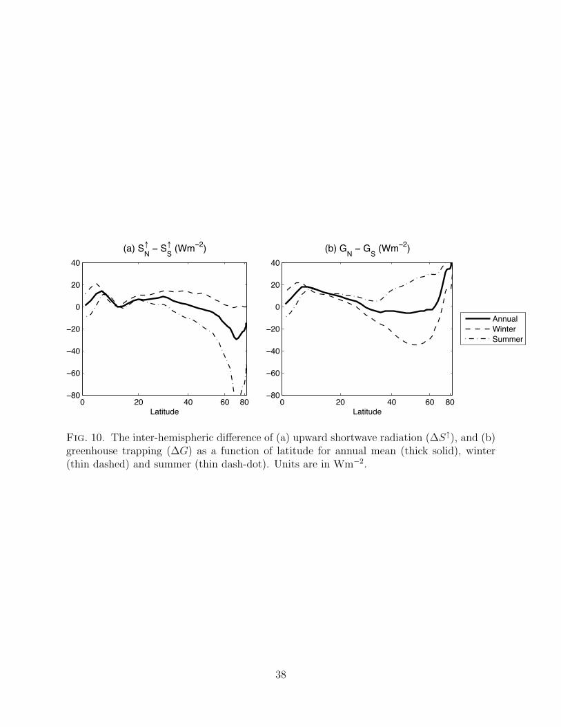
The latitudinal structures of the inter-hemispheric differences in upward TOA shortwave

radiation and greenhouse trapping are shown in Fig. 10 and that of cloud cover in Fig. 11. In

summer seasons, the NH reflects less SW than the SH in the mid- to high latitudes, despite

ice-free land albedo being larger than ocean albedo, due to less cloud cover (Fig. 11) and

the high albedo Antarctic ice sheet. In winter seasons, the NH reflects more partly due to

snow cover over land poleward of 40◦. However there is also more SW reflection in the NH

between 15◦ and 40◦ even though cloud cover is less in the NH all year long (Fig. 11). The

SW reflection is larger in the NH equatorward of 15◦ because of clouds associated with the

NH ITCZ.

The gross features of the latitudinal structure in the inter-hemispheric difference in green-

house trapping (Fig. 10) are well correlated with those in surface temperatures (Fig. 2a),

except the local maxima in the deep tropics where there is little temperature differences.

The peak in greenhouse trapping in the tropics is due to a super greenhouse effect, whereby

greenhouse trapping increases with surface temperature so strongly that OLR actually de-

creases as the surface warms (Raval and Ramanathan 1989). During winter seasons the

smaller greenhouse trapping in the NH in the mid- to high latitudes is due to drying and

cooling of the continents. The opposite occurs in summer seasons. The map of annual mean

13

greenhouse trapping overlain with surface temperature (Fig. 12) clearly indicates that these

are well correlated. However, it is not clear which is the cause and which is the effect.

On the face of it then the NH is warmer than the SH because of the greater greenhouse

trapping in the NH. This is in contrast with Croll�s expectation that the hemisphere with

more ocean would have the greater trapping and be warmer were it not for ocean heat export

from the SH to the NH. However it could be that the greater greenhouse trapping in the NH

is not the cause of that hemisphere being warmer but a consequence, via the positive water

vapor-greenhouse feedback, of the ocean heat export warming the NH relative to the SH.

5. A Simple Model of Inter-hemispheric Temperature

Asymmetry

To examine whether inter-hemispheric differences in G are causes or effects of inter-

hemispheric differences in T , a simple box model is used that solves for ∆T from the energy

budget, as depicted in Fig. 13. The model conceptually follows those in Ramanathan and

Collins (1991) and Sun and Liu (1996). Two boxes with temperatures TS and TN respectively

represent the SH and the NH. At TOA, there is net shortwave radiation S and outgoing

longwave radiation F . For simplicity, the net shortwave radiation S is considered to be the

same for the two hemispheres by taking the global mean of S0=239.5 Wm−2. Since differences

in S are small, taking the actual values for the respective hemisphere, SS and SN makes little

difference. The OLR is given by F = σT 4 − G where σ=5.67×10−8 Wm−2K−1 and G is

the greenhouse trapping. The northward oceanic transport FO is prescribed, but due to its

14

uncertainties a range of values from 0 to 1.10 PW is used (Section 4a). The atmospheric

transport FA is thermally direct and parameterized as a function of ∆T = TN − TS, i.e.

FA = ∂FA∂∆T

∆T . The annual mean values of FA and ∆T at the equator from NCEP/NCAR

reanalysis between 1979 and 2007 are used to compute the coefficient, ∂FA∂∆T

, referred to as

the strength of atmospheric transport, by regressing FA onto ∆T , yielding the value of -0.20

PW K−1. To express atmospheric and oceanic energy transport in a flux form in Wm−2, FA

and FO are divided by the hemispheric mean area, A0. The energy budget for the two boxes

can be written as:

S0 − σT 4S

+ GS − FO/A0 +

����∂FA/A0

∂∆T

���� ∆T = 0 (3)

S0 − σT 4N

+ GN + FO/A0 −����∂FA/A0

∂∆T

���� ∆T = 0 (4)

The above equations can be linearized by applying the first-order Taylor expansion around

global mean values denoted by the subscript 0 as:

S0 − {σT 40 + 4σT 3

0 (TS − T0)}+ {G0,S +∂G

∂T(TS − T0)}− FO/A0 +

����∂FA/A0

∂∆T

���� ∆T = 0 (5)

S0 − {σT 40 + 4σT 3

0 (TN − T0)}+ {G0,N +∂G

∂T(TN − T0)}+ FO/A0 −

����∂FA/A0

∂∆T

���� ∆T = 0 (6)

Note that G is linearized at different basic states in each hemisphere (G0,S and G0,N), in

recognition of potential differences in thermal characteristics between the two hemispheres

not caused by the temperature difference but imposed by differences in fractional coverage of

ocean, continental arrangements, etc. For example, G0,N could be larger than G0,S, despite

greater ocean fraction in the south, because subtropical dry regions over the ocean are more

developed in the SH than the NH and due to massive humidity in Asia associated with the

summer monsoon.

15

By adding the two equations, we get a constraint on the global mean greenhouse effect,

(G0,S+G0,N)/2 = σT 40−S0 (=288.8 Wm−2) where T0 is the global-mean annual-mean surface

temperature of 14.8◦C. Eqs. (5) and (6) can be expressed in terms of one unknown, ∆T :

�2σT 3

0 −1

2

∂G

∂T+

����∂FA/A0

∂∆T

����

�∆T = FO/A0 + ∆G0/2. (7)

∆G0 ≡ G0,N − G0,S is the basic state G difference between the hemispheres. ∂G

∂T(=4.0

Wm−2K−1), referred to as the greenhouse trapping efficiency, is estimated as 4σT 30 − ∂F

∂T

where ∂F

∂T(=1.5 Wm−2K−1) is the regression coefficient relating the monthly anomaly of

global mean OLR to that of T using surface temperature from NCEP/NCAR reanalysis and

OLR from CERES data between 2001 and 2004.

The model results for ∆T from Eq. (7) as a function of FO for the case with ∆G0=0

are plotted in Fig. 14a. The shading indicates the one standard deviation of observed ∆T

from its global mean. The realistic solutions are those that fall within the shaded area.

The reference state with the most reasonable estimates of parameters, ∂G

∂T=4.0 Wm−2K−1

and ∂FA∂∆T

=0.20 Wm−2K−1, is plotted in black and requires large northward FO of about 0.57

PW to fall in the realistic range of ∆T . When there is no cross-equatorial transport by the

atmosphere (blue), ∆T increases and deviates from the realistic range for a cross-equatorial

FO greater than 0.2PW, suggesting that the atmosphere acts to reduce the inter-hemispheric

contrast. When the greenhouse trapping efficiency increases (red), the inter-hemispheric

difference gets larger via positive water vapor feedback for a given FO as the warmer NH

gets even warmer and the cooler SH cools more. The resulting inter-hemispheric difference

of greenhouse trapping, ∆G for a given ∆T is displayed in Fig. 14b. Here the horizontal

shading shows the range of the observed ∆G. Because ∆G is determined by ∂G

∂Tand ∆T , it

16

changes only when the efficiency ∂G

∂Tvaries for a given ∆T , hence, the lines representing cases

with (black) and without (blue) atmosphere heat transport are overlapped. The greenhouse

trapping contrast increases with larger ∆T or as its efficiency gets larger. In the cases with

a realistic range of ∆T , the reference state including atmospheric energy transport yields

∆G that is at the margin of the observed range.

In the box model with the same basic state G in each hemisphere, the northward oceanic

transport is the only mechanism that can produce a warmer NH. However, the magnitude of

northward OHT needed for realistic solutions appears larger than the data supports (Section

4a). Hence, we consider the case with nonzero ∆G0, since not all of ∆G in Fig. 9 need be a

result of ∆T , but could be in part due to basic state differences as suggested in Fig. 6 and

discussed above. The model solutions for FO=0 as a function of ∆G0 are shown in Figs. 14c

and 14d. For the reference solution (black) to be in the realistic ∆T range, it requires ∆G0 ≈

4 Wm−2, which then yields ∆G ≈ 9 Wm−2, much larger than the real value of 5.67 Wm−2.

That is, with no ocean heat transport, too large of an inter-hemispheric difference of G is

needed to obtain the right magnitude of ∆T . We therefore consider a combination of the first

two models that takes into account both FO and ∆G0. Figs. 14e and 14f show the solutions

for FO=0.3 PW, which is within the range in Fasullo and Trenberth (2008b), as a function

of ∆G0. The realistic ∆T is obtained for ∆G0 ≈ 1.5 Wm−2, which then yields ∆G within

the realistic range of about 6.0Wm−2.

For plausible magnitudes of northward OHT, positive ∆G0, greenhouse trapping effi-

ciency and atmospheric heat transport strength, the box model does predict values of ∆T

and ∆G that are consistent with those observed. Therefore the model supports the idea

that a northward cross-equatorial OHT is required for the inter-hemispheric temperature

17

difference on Earth, as Croll suggested.

6. Discussion

The box model based on the TOA energy budget suggests that the necessary factors for

the warmer NH than the SH are:

• a northward cross-equatorial ocean heat transport

• a larger basic state greenhouse effect in the north

The larger annual-mean inter-hemispheric difference in the Atlantic sector (5.2◦C) than in the

Pacific sector (2.5◦C) (Fig. 8) supports this idea because the northward cross-equatorial OHT

occurs in the Atlantic Ocean (e.g. see Fig. 9 in Trenberth and Fasullo 2008). That is, the

ocean transports energy northward, the NH gets warmer and this inter-hemispheric difference

is enhanced by greenhouse trapping. Since the tropical mean atmospheric circulation is

thermally direct, the inter-hemispheric temperature difference is partly compensated by the

atmospheric energy transport from the north to the south which is associated with the mean

ITCZ being in the north (Kang et al. 2008, 2009).

However, the quality of ocean data is insufficient for deriving not only the magnitude but

also the direction of cross-equatorial OHT. For the inter-hemispheric temperature difference

to be entirely caused by northward cross-equatorial OHT a value (∼0.6PW) at the very

upper limit of the observational range is required. A more reasonable OHT is inferred if

some portion of the inter-hemispheric temperature difference arises from a difference in the

basic state greenhouse trapping, i.e. some aspect of the atmospheric circulation and humidity

18

distribution that creates more greenhouse trapping in the NH than the SH independent of the

temperature difference. However, since the greenhouse effect incorporates efficient positive

feedback, it is difficult to extract this postulated basic state difference between the two

hemispheres.

Only much more accurate OHT data, presumably obtained through combinations of in-

situ data, atmospheric and oceanic Reanalyses, satellite data and adjoint methods, will be

able to settle the contribution of cross-equatorial OHT to the inter-hemispheric temperature

difference. The issue of a postulated inter-hemispheric difference in basic state greenhouse

trapping would most likely be best addressed with idealized climate modeling.

7. Conclusions

We have discussed why the NH is warmer than the SH in the annual mean and pursued

the idea, put forth by Croll (1870), that it is caused by northward cross-equatorial OHT.

Croll (1870) claimed that the hemisphere with the larger ocean fraction would be warmer

because of higher humidity, and hence, more greenhouse trapping. It is true that the ocean is

warmer than land at every latitude in the annual mean. However, we find that the greenhouse

trapping is in fact larger over land than ocean at the same temperature. The reason for the

warmer ocean is, instead, the smaller surface albedo of the ocean. Therefore the larger land

fraction in the north acts to cool the NH relative to the SH. This effect is offset by the fact

that both the NH land masses and the NH oceans are warmer than their SH counterparts.

Of these it is the warmer ocean in the north that contributes most to preferentially

warming the NH. A simple box model based on the energy budget shows that in order to

19

obtain an inter-hemispheric temperature difference within the observed range an unrealisti-

cally large greenhouse trapping difference is needed if there is no ocean transport across the

equator. On the other hand, unrealistically large northward cross-equatorial ocean trans-

port is needed for the case with no basic static greenhouse trapping difference between the

two hemispheres. The most reasonable solution combines a modest northward OHT and

an inter-hemispheric difference in the basic state greenhouse trapping. Hence, the greater

greenhouse trapping in the NH (by 5.7 Wm−2) is not the main cause of the warmer north

but more of a consequence, and the northward oceanic heat transport is critical to produc-

ing a warmer NH, consistent with Croll (1870). We also suggest that the inter-hemispheric

temperature difference is contributed to by an inter-hemispheric difference in the basic state

greenhouse trapping. This inter-hemispheric temperature difference created by these mech-

anisms is enhanced by the positive water vapor-greenhouse feedback. The thermally direct

tropical mean atmospheric circulation then partly compensates for this inter-hemipsheric

contrast by transporting energy southward in association with the ITCZ in the NH.

It is normally assumed that the northward oceanic heat transport, which occurs in the

Atlantic Ocean, is a result of the deep Atlantic meridional overturning circulation with north-

ward surface flow, sinking in the North Atlantic and southward flow at depth and upwelling

around Antarctica and it can be reproduced in this way easily in idealized models (Togg-

weiler and Bjornsson 2000). As such, it is a consequence of the arrangement of continents

and oceans on the planet that enable the Atlantic Ocean to be saltier than the Pacific Ocean

(Emile-Geay et al. 2003). On the other hand it has not to our knowledge been demonstrated

that Atlantic cross-equatorial OHT could not exist in the absence of the deep overturning

circulation just as it does (to the south) in the Indian Ocean. Consequently a definitive

20

account of why the NH is warmer than the SH requires a thorough accounting for the causes

of the cross-equatorial OHT because, as shown here, this is a fundamental cause of the

asymmetry.

However, unless estimates of cross-equatorial OHT are highly inaccurate, it is unlikely

that this is the sole cause of the inter-hemispheric temperature difference. An inter-hemispheric

difference in greenhouse trapping appears to be a probable additional cause. This would

likely be a result of how the arrangement of continents, and its impact on atmosphere-ocean

circulation features such as monsoons, subtropical anticyclones and ocean upwelling regions,

determines the distribution of atmospheric water vapor. To assess if this is so will require

much more research including the use of idealized and comprehensive climate models.

The fact that the NH is warmer than the SH is potentially linked to the fact that the

ITCZ is in the NH (Kang et al. 2008). The mechanisms for the inter-hemispheric temperature

difference are such that we would expect the difference to change as a result of radiatively-

forced climate change and, hence, influence the ITCZ position. Millions of the world’s

population depend on ITCZ rains for their water and food making the problem of how ITCZ

location is determined one of great social relevance. It is sobering that the current state of

observations of the Earth’s climate system is inadequate to fully answer such a fundamental

question as why the NH is warmer than the SH and, hence provide a full account of why

tropical rain belts are where they are.

Acknowledgments.

We thank David Battisti for useful discussions that initiated this work. Also, John

21

Fasullo’s help in interpreting the OHT data is greatly appreciated. RS was supported by

NSF award AGS 08-04107.

22

REFERENCES

Croll, J., 1870: XII. On Ocean-currents, Part I: Ocean-currents in relation to the Distribution

of Heat over the Globe. Philosophical Magazine and Journal of Science, 39 (259), 81–106.

Emile-Geay, J., M. A. Cane, N. Naik, R. Seager, A. C. Clement, and A. van Geen, 2003:

Warren revisited: Atmospheric freshwater fluxes and why is no deep water formed in the

north pacific. J. Geophys. Res., 108, 3178.

Fasullo, J. T. and K. E. Trenberth, 2008a: The annual cycle of the energy budget. Part I:

Global mean and land-ocean exchanges. Journal of Climate, 21 (10), 2297–2312.

Fasullo, J. T. and K. E. Trenberth, 2008b: The annual cycle of the energy budget. Part II:

Meridional structures and poleward transports. Journal of Climate, 21 (10), 2313–2325.

Kang, S. M., D. M. W. Frierson, and I. M. Held, 2009: The tropical response to extratropical

thermal forcing in an idealized gcm: The importance of radiative feedbacks and convective

parameterization. Journal of the Atmospheric Sciences, 66 (9), 2812–2827.

Kang, S. M., I. M. Held, D. M. W. Frierson, and M. Zhao, 2008: The response of the ITCZ

to extratropical thermal forcing: Idealized slab-ocean experiments with a GCM. Journal

of Climate, 21 (14), 3521–3532.

Kistler, R. and Coauthors, 2001: The NCEP–NCAR 50–Year Reanalysis: Monthly Means

CD–ROM and Documentation. Bull. Amer. Meteor. Soc., 82, 247–267.

23

Loschnigg, J. and P. J. Webster, 2000: A Coupled Ocean–Atmosphere System of SST Mod-

ulation for the Indian Ocean. J. Climate, 13, 3342–3360.

Meehl, G. A., C. Covey, T. Delworth, M. Latif, B. McAvaney, J. F. B. Mitchell, R. J.

Stouffer, and K. E. Taylor, 2007: The WCRP CMIP3 multimodel dataset. Bull. Am.

Meteorol. Soc., 88, 1383–1394.

Philander, S. G. H., D. Gu, G. Lambert, T. Li, D. Halpern, N.-C. Lau, and R. C. Pacanowski,

1996: Why the ITCZ Is Mostly North of the Equator. Journal of Climate, 9 (12), 2958–

2972.

Ramanathan, V. and W. Collins, 1991: Thermodynamic regulation of ocean warming by

cirrus clouds deduced from observations of the 1987 El Nino. Nature, 351, 27–32.

Raval, A. and V. Ramanathan, 1989: Observational determination of the greenhouse effect.

Nature, 342, 758–761.

Rodwell, M. J. and B. J. Hoskins, 2001: Subtropical anticyclones and summer monsoons. J.

Climate, 14, 3192–3211.

Rossow, W. B. and R. A. Schiffer, 1991: ISCCP cloud datasets. Bull. Amer. Meteor. Soc.,

72, 2–20.

Seager, R., R. Murtugudde, N. Naik, A. Clement, N. Gordon, and J. Miller, 2003: Air–

Sea Interaction and the Seasonal Cycle of the Subtropical Anticyclones*. J. Climate, 16,

1948–1966.

24

Sun, D.-Z. and Z. Liu, 1996: Dynamic Ocean-Atmosphere Coupling: A Thermostat for the

Tropics. Science, 272, 1148–1150.

Toggweiler, J. R. and H. Bjornsson, 2000: Drake Passage and palaeoclimate. Journal of

Quaternary Science, 15 (4), 1099–1417.

Trenberth, K. E. and J. T. Fasullo, 2008: An observational estimate of inferred ocean energy

divergence. Journal of Physical Oceanography, 38 (5), 984–999.

Uppala, S. M. and Coauthors, 2005: The ERA-40 reanalysis. Quart. J. Roy. Meteor. Soc.,

131, 2961–3012.

Wielicki, B. A., B. R. Barkstrom, E. F. Harrison, R. B. Lee, G. L. Smith, and J. E. Cooper,

1996: Clouds and the Earth’s Radiant Energy System (CERES): An Earth Observing

System experiment. Bull. Amer. Meteor. Soc., 77, 853–868.

25

List of Figures

1 The hemispheric mean (a) surface temperature, (b) ocean temperature, and

(c) land temperature in the north (dotted) and the south (hatching) for annual

mean, winter (DJF for the NH and JJA for the SH) and summer (JJA for the

NH and DJF for the SH). Units are in ◦C. 29

2 The inter-hemispheric difference of (a) surface temperature, (b) ocean tem-

perature, and (c) land temperature as a function of latitude for annual mean

(thick solid), winter (thin dashed) and summer (thin dash-dot). Units are

in ◦C. The x coordinate is linear in sine of latitude so that equal spacing

corresponds to equal surface area on the globe. 30

3 The schematic figure of hemispheric mean temperatures of surface, ocean, and

land for annual mean (green), winter (blue) and summer (red) and fractions

of ocean (fO) and land (fL) cover. 31

4 The inter-hemispheric difference of surface temperature (hatching, ∆T ), the

fraction of ∆T resulting from differences in ocean temperatures (dotted), land

temperatures (horizontal lines), and ocean fraction (crossing) for annual mean,

winter and summer. Units are in ◦C. 32

5 The latitudinal difference between ocean and land of (a) temperatures T (in

◦C), (b) greenhouse trapping, G (in Wm−2), and (c) upward shortwave radi-

ation at TOA, SW ↑ (in Wm−2) for annual mean (thick solid), winter (thin

dashed) and summer (thin dash-dot). 33

26

6 The greenhouse trapping G (in W) for a given temperature T (in ◦C) over

land in solid and over ocean in dashed. 34

7 The annual mean inter-hemispheric difference of upward shortwave radiation

at TOA (∆S↑), the fraction of ∆S↑ resulting from the inter-hemispheric dif-

ference over ocean fO,N∆S↑O, over land (1 − fO,S)∆S↑

L, and from the inter-

hemispheric difference in ocean fraction (fO,S − fO,N)(S↑L,N

−S↑O,S

). Units are

in Wm−2. 35

8 The inter-hemispheric ocean temperature difference in the Atlantic (hatching),

Pacific (dotted), and Indian (crossing) for each season. ∆TO in the Pacific and

the Atlantic are computed as the TO difference between (0–60◦N) and (60◦S–

0) at each basin, and in the Indian Ocean the difference is taken between

(0–20◦N) and (20◦S–0). 36

9 The inter-hemispheric difference of downward shortwave radiation (∆S↓), up-

ward shortwave radiation (∆S↑), and greenhouse trapping (∆G) for annual

mean (hatching), winter (dotted) and summer (crossing). Units are in Wm−2. 37

10 The inter-hemispheric difference of (a) upward shortwave radiation (∆S↑),

and (b) greenhouse trapping (∆G) as a function of latitude for annual mean

(thick solid), winter (thin dashed) and summer (thin dash-dot). Units are in

Wm−2. 38

11 The inter-hemispheric difference of cloud fraction with latitude for annual

mean (thick solid), winter (thin dashed) and summer (thin dash-dot). 39

27

12 The global map of annual mean surface temperature (in ◦C) in black contour

and greenhouse trapping (in Wm−2) in color shading. The contour interval is

4◦C and shading interval is 10 Wm−2. 40

13 The schematic figure for the box model based on energy budget. The net

incoming shortwave radiation S is balanced by outgoing longwave radiation

F , meridional energy transports by atmosphere FA and ocean FO. The model

solves for surface temperature T . The subscripts N and S denote the hemi-

spheric mean in the north and the south, respectively. 41

14 Solutions from the box model: the inter-hemispheric difference of (a) surface

temperature (∆T = TN −TS, in ◦C) as a function of prescribed oceanic trans-

port FO (in PW), and (b) greenhouse trapping (∆G = GN − GS, in Wm−2)

as a function of ∆T for the case with no basic state G difference (∆G0=0).

(c,d) Same as (a,b) but as a function of ∆G0(= G0,N − G0,S) for no oceanic

transport (FO=0). (e,f) Same as (c,d) but for the case with FO=0.3PW.

The reference state (black) is the solution with the most reasonable param-

eters, ∂G

∂T=4.0Wm−2K−1 and ∂FA

∂∆T=0.20Wm−2K−1. Blue is the case with no

cross-equatorial atmospheric heat transport ∂FA∂∆T

=0 and red is with stronger

greenhouse trapping ∂G

∂T=5.0Wm−2K−1. Black dashed lines denotes the an-

nual mean values, and the gray shading denotes the one standard deviation

of observed ∆T and ∆G. 42

28

Fig. 1. The hemispheric mean (a) surface temperature, (b) ocean temperature, and (c) landtemperature in the north (dotted) and the south (hatching) for annual mean, winter (DJFfor the NH and JJA for the SH) and summer (JJA for the NH and DJF for the SH). Unitsare in ◦C.

29

! "! #! $! %!!"!

!&!

!

&!

"!

'!

()*+,-+!+,

.+(°/*

+

+

0112)3

451678

.29978

! "! #! $! %!!"!

!&!

!

&!

"!

'!

:)6562;7

(<*+,=>-+!+,

=>.+(°/*

! "! #! $! %!!"!

!&!

!

&!

"!

'!

:)6562;7

(?*+,:>-+!+,

:>.+(°/*

Fig. 2. The inter-hemispheric difference of (a) surface temperature, (b) ocean temperature,and (c) land temperature as a function of latitude for annual mean (thick solid), winter (thindashed) and summer (thin dash-dot). Units are in ◦C. The x coordinate is linear in sine oflatitude so that equal spacing corresponds to equal surface area on the globe.

30

Fig. 3. The schematic figure of hemispheric mean temperatures of surface, ocean, and landfor annual mean (green), winter (blue) and summer (red) and fractions of ocean (fO) andland (fL) cover.

31

Fig. 4. The inter-hemispheric difference of surface temperature (hatching, ∆T ), the fractionof ∆T resulting from differences in ocean temperatures (dotted), land temperatures (hori-zontal lines), and ocean fraction (crossing) for annual mean, winter and summer. Units arein ◦C.

32

!!" !#" " #" !"!$"

"

$"

%"

#"

&'()(*+,

-'./01!0

&/-!2.

/

/

344*'5

6)4(,7

8*99,7

!!" !#" " #" !"

!!"

!#"

"

#"

!"

&'()(*+,

-:./;1!;

&/-69

!%.

!!" !#" " #" !"

!!"

!#"

"

#"

!"

&'()(*+,

-<./8!

1!8

!

&/-69

!%.

Fig. 5. The latitudinal difference between ocean and land of (a) temperatures T (in ◦C),(b) greenhouse trapping, G (in Wm−2), and (c) upward shortwave radiation at TOA, SW ↑

(in Wm−2) for annual mean (thick solid), winter (thin dashed) and summer (thin dash-dot).

33

!!" !#" !$" !%" !&" !'" !(" " (" '" &" %"

"

'

%

#

)

("

('*+("

('

,+-°./

0+-1/

+

+

2345

67834

Fig. 6. The greenhouse trapping G (in W) for a given temperature T (in ◦C) over land(solid) and over ocean (dashed).

34

!!

!"#$

!"

!%#$

%

%#$

"

"#$

!

!#$

&

!'" (

)*+!'

"

),"!(

)*'-!'

"

.,()*'!()*+-,'

"

.*+!'

"

)*'-

/012345624017207'"

+!'

"

'7,89

!!-

7

7

Fig. 7. The annual mean inter-hemispheric difference of upward shortwave radiation atTOA (∆S↑), the fraction of ∆S↑ resulting from the inter-hemispheric difference over oceanfO,N∆S↑

O, over land (1− fO,S)∆S↑

L, and from the inter-hemispheric difference in ocean frac-

tion (fO,S − fO,N)(S↑L,N

− S↑O,S

). Units are in Wm−2.

35

Fig. 8. The inter-hemispheric ocean temperature difference in the Atlantic (hatching),Pacific (dotted), and Indian (crossing) for each season. ∆TO in the Pacific and the Atlanticare computed as the TO difference between (0–60◦N) and (60◦S–0) at each basin, and in theIndian Ocean the difference is taken between (0–20◦N) and (20◦S–0).

36

Fig. 9. The inter-hemispheric difference of downward shortwave radiation (∆S↓), upwardshortwave radiation (∆S↑), and greenhouse trapping (∆G) for annual mean (hatching),winter (dotted) and summer (crossing). Units are in Wm−2.

37

! "! #! $! %!!%!

!$!

!#!

!"!

!

"!

#!

&'()(*+,

-'./0!

1/!/0

!

0/-23

!".

! "! #! $! %!!%!

!$!

!#!

!"!

!

"!

#!

&'()(*+,

-4./51/!/5

0/-23

!".

/

/

677*'8

2)7(,9

0*33,9

Fig. 10. The inter-hemispheric difference of (a) upward shortwave radiation (∆S↑), and (b)greenhouse trapping (∆G) as a function of latitude for annual mean (thick solid), winter(thin dashed) and summer (thin dash-dot). Units are in Wm−2.

38

! "! #! $! %!

!!&"

!!&'

!

!&'

!&"

!&(

!&#

!&)

*+,-,./0

123./456+7,-384/-55060870

4

4

988.+2

:-8,06

;.<<06

Fig. 11. The inter-hemispheric difference of cloud fraction with latitude for annual mean(thick solid), winter (thin dashed) and summer (thin dash-dot).

39

!"#$%&'()

!*&%&'()

+##'*,-.)*#-/-0°12-*#(-3-04.

!52

-

-

67 857 897 5:7 ;77

!97

!67

!:7

!57

7

57

:7

67

97

7

<7

877

8<7

577

Fig. 12. The global map of annual mean surface temperature (in ◦C) in black contour andgreenhouse trapping (in Wm−2) in color shading. The contour interval is 4◦C and shadinginterval is 10 Wm−2.

40

Fig. 13. The schematic figure for the box model based on energy budget. The net incomingshortwave radiation S is balanced by outgoing longwave radiation F , meridional energytransports by atmosphere FA and ocean FO. The model solves for surface temperatureT . The subscripts N and S denote the hemispheric mean in the north and the south,respectively.

41

! !"# !"$ !"% !"& '!

!"(

'

'"(

#

#"(

)

*+,-./0

12!13,-!40

-50,!6!7!

!

#

$

%

&

'!

! !"( ' '"( # #"(

62!63,-/8!#0

12!1

3,-!40

-90,!6!7!

! ' # ) $ (!

!"(

'

'"(

#

#"(

)

6!:2!6

!:3,-/8

!#0

12!13,-!40

-;0,*+7!"!,./

!

#

$

%

&

'!

! !"( ' '"( # #"(

62!63,-/8!#0

12!1

3,-!40

-<0,*+7!"!,./

! ' # ) $ (!

!"(

'

'"(

#

#"(

)

6!:2!6

!:3,-/8

!#0

12!13,-!40

-=0,*+7!"),./

!

#

$

%

&

'!

! !"( ' '"( # #"(

62!63,-/8!#0

12!1

3,-!40

->0,*+7!"),./

,

,

"6?"17$:,"*@?"!17!"#

"6?"17$:,"*@?"!17!

"6?"17(:,"*@?"!17!"#

Fig. 14. Solutions from the box model: the inter-hemispheric difference of (a) surfacetemperature (∆T = TN − TS, in ◦C) as a function of prescribed oceanic transport FO (inPW), and (b) greenhouse trapping (∆G = GN − GS, in Wm−2) as a function of ∆T forthe case with no basic state G difference (∆G0=0). (c,d) Same as (a,b) but as a functionof ∆G0(= G0,N − G0,S) for no oceanic transport (FO=0). (e,f) Same as (c,d) but for thecase with FO=0.3PW. The reference state (black) is the solution with the most reasonableparameters, ∂G

∂T=4.0Wm−2K−1 and ∂FA

∂∆T=0.20Wm−2K−1. Blue is the case with no cross-

equatorial atmospheric heat transport ∂FA∂∆T

=0 and red is with stronger greenhouse trapping∂G

∂T=5.0Wm−2K−1. Black dashed lines denotes the annual mean values, and the gray shading

denotes the one standard deviation of observed ∆T and ∆G.

42