Embed Size (px)
Citation preview

Contribution au developpement de methodologies pour
l’Automatique fondees sur l’optimisation
Guillaume Sandou
To cite this version:
Guillaume Sandou. Contribution au developpement de methodologies pour l’Automatiquefondees sur l’optimisation. Automatique / Robotique. Universite Paris Sud - Paris XI, 2012.<tel-00707124>
HAL Id: tel-00707124
https://tel.archives-ouvertes.fr/tel-00707124
Submitted on 12 Jun 2012
HAL is a multi-disciplinary open accessarchive for the deposit and dissemination of sci-entific research documents, whether they are pub-lished or not. The documents may come fromteaching and research institutions in France orabroad, or from public or private research centers.
L’archive ouverte pluridisciplinaire HAL, estdestinee au depot et a la diffusion de documentsscientifiques de niveau recherche, publies ou non,emanant des etablissements d’enseignement et derecherche francais ou etrangers, des laboratoirespublics ou prives.
Mémoire
Présenté pour obtenir
L’HABILITATION A DIRIGER DES RECHERCHES
Contribution au développement de méthodologies pour l’Automatique fondées sur l’optimisation
par
Guillaume SANDOU
Supélec Sciences des Systèmes (E3S) – Département Automatique
Soutenue le 1er juin 2012 devant la Commission d’examen :
MM. Philippe CHEVREL Ecole des Mines de Nantes Examinateur Gilles DUC Supélec Examinateur Luc DUGARD GIPSA-Lab CNRS Rapporteur Jin-Kao HAO LERIA, Université d’Angers Rapporteur Jean-Philippe HARCAUT MBDA Examinateur Silviu-Iulian NICULESCU L2S CNRS Examinateur Vincent WERTZ Université Catholique de Louvain Rapporteur Michel ZASADZINSKI Université de Lorraine Président


A Sophie, Mélina et Bastien


Remerciements
Ce mémoire correspond au travail effectué durant une dizaine d’années au sein du
Département Automatique de Supélec. Les occasions de remercier les personnes de mon
entourage sont trop rares pour que je ne profite de celle qui m’est donnée ici.
Tout d’abord j’adresse mes plus vifs remerciements aux perspicaces ressources humaines d’une
entreprise française du secteur de l’automobile pour avoir refusé en 2002 ma candidature en
thèse. A posteriori, ce fut le plus merveilleux échec qui soit, la conséquence étant mon arrivée
au Département Automatique de Supélec. Je remercie Patrick Boucher, chef du Département,
pour m’avoir fait confiance à cette époque.
Je remercie les membres du jury pour le temps qu’ils m’ont consacré, à savoir Luc Dugard, Jin-
Kao Hao et Vincent Wertz qui ont accepté la charge, je l’espère pas trop désagréable, de
rapporteur de mes travaux, ainsi que Philippe Chevrel, Gilles Duc, Jean-Philippe Harcaut, Silviu
Niculescu et Michel Zasadzinski.
J’adresse toutes mes amitiés à Dominique Beauvois, Elisabeth Boillot, Patrick Boucher, Josiane
Dartron, Martial Demerlé, Gilles Duc, Didier Dumur, Stéphane Font, Emmanuel Godoy, Léon
Marquet, Sorin Olaru, Pedro Rodriguez, Sihem Tebbani, tous membres du Département
Automatique, certes pour l’excellente ambiance de travail, les collaborations fructueuses et les
discussions, mais également pour les bières et spécialités locales que nous avons pu déguster
ensemble. Je n’oublie pas également les membres d’autres départements de l’école, nos
collègues de l’équipe d’Automatique de Rennes, ainsi que tous les doctorants et stagiaires que
j’ai pu côtoyer.
Je ne saurais terminer cette page sans une pensée plus qu’affectueuse pour mon épouse Sophie
et nos enfants Mélina et Bastien, qui ont la lourde de charge de supporter un enseignant
chercheur souvent occupé et préoccupé, et qui contribuent, chacun à leur façon, à la
préservation de ma santé mentale.


i
Table des matières
Première partiePremière partiePremière partiePremière partie : présentation du candidat: présentation du candidat: présentation du candidat: présentation du candidat 1111
Chapitre 1 Curriculum Vitae détaillé ................................................................................ 3
1.1. Présentation du candidat ...................................................................................... 5
1.1.1. Etat civil ............................................................................................................ 5
1.1.2. Formation .......................................................................................................... 5
1.1.3. Expérience professionnelle ............................................................................... 6
1.2. Activités d’enseignement ...................................................................................... 6
1.2.1. Activités d’enseignement actuelles à Supélec .................................................. 6
1.2.1.1. Cours magistraux ...................................................................................... 7
1.2.1.2. Travaux Dirigés ........................................................................................ 8
1.2.1.3. Etudes de Laboratoire et projets ............................................................... 8
1.2.1.4. Responsabilités en matière d’enseignement ............................................. 9
1.2.1.5. Bilan chiffré des activités d’enseignement à Supélec .............................. 9
1.2.2. Activités d’enseignement en tant que vacataire ............................................... 9
1.2.2.1. Activités d’enseignement à l’Ecole des Mines de Nantes ........................ 9
1.2.2.2. Activités d’enseignement à l’Ecole Nationale Supérieure de Techniques Avancées (ENSTA) ............................................................................................. 10
1.2.2.3. Activités d’enseignement à l’Ecole Centrale de Paris ........................... 11
1.2.2.4. Activités d’enseignement à l’Université d’Evry-Val d’Essonne ........... 11
1.2.2.5. Activités d’enseignement à l’Ecole Militaire ......................................... 11
1.2.2.6. Bilan chiffré des activités d’enseignement en tant que vacataire ........... 11
1.2.3. Activités d’enseignement passées .................................................................. 11
1.3. Activités de recherche ......................................................................................... 13
1.3.1. Introduction et motivations ............................................................................. 13
1.3.2. Modélisation, optimisation et commande de systèmes industriels ................. 14
1.3.2.1. Domaine de l’énergie ............................................................................. 14
1.3.2.2. Domaine automobile .............................................................................. 15
1.3.2.3. Domaine aéronautique ............................................................................ 16
1.3.2.4. Activités « inclassables » ....................................................................... 16
1.3.2.5. Bilan méthodologique ............................................................................ 16
1.3.3. Développement de méthodes génériques pour l’Automatique fondées sur les métaheuristiques ....................................................................................................... 17
1.3.3.1. Identification de systèmes ...................................................................... 17

ii
1.3.3.2. Optimisation de correcteurs. .................................................................. 17
1.3.3.3. Synthèse H∞ ............................................................................................ 18
1.3.4. Transfert de méthodologies vers l’industrie ................................................... 18
1.3.4.1. Optimisation de l’affectation d’unités .................................................... 18
1.3.4.2. Utilisation d’algorithmes d’optimisation métaheuristiques ................... 19
1.3.4.3. Commande prédictive ............................................................................ 19
1.4. Participation à la vie scientifique ....................................................................... 20
1.4.1. Au sein de Supélec ......................................................................................... 20
1.4.2. Rayonnement extérieur ................................................................................... 21
1.4.2.1. Collaborations et projets de recherche internationaux ........................... 21
1.4.2.2. Collaborations scientifiques nationales .................................................. 22
1.4.2.3. Participations à des groupes de travail ................................................... 23
1.4.2.4. Activités de relecture .............................................................................. 23
1.4.2.5. Participation à des comités de programme ............................................. 24
1.4.2.6. Présidence de session dans des conférences internationales .................. 24
1.5. Encadrement d’étudiants (doctorants, post-doctorat stagiaires et élèves ingénieurs) .................................................................................................................. 25
1.5.1. Encadrement de thèses soutenues ................................................................... 25
1.5.2. Encadrement de thèse en cours ....................................................................... 25
1.5.3. Encadrement de post-doctorant…… ………………………………………26
1.5.4. Encadrement de stages de master ................................................................... 26
1.5.5. Encadrement de stages de fin d’étude ............................................................ 27
1.5.6. Encadrement d’élèves ingénieurs dans le cadre de Contrats d’Etude Industrielle .................................................................................................................................. 28
1.6. Collaborations industrielles ............................................................................... 29
1.7. Liste de publications ........................................................................................... 30
1.7.1. Chapitres d’ouvrage ........................................................................................ 30
1.7.2. Articles de revue internationale à comité de lecture ....................................... 32
1.7.3. Brevet .............................................................................................................. 32
1.7.4. Conférences internationales avec actes .......................................................... 33
1.7.5. Conférences internationales sans actes ........................................................... 35
1.7.6. Conférences nationales ................................................................................... 35
1.7.7. Communications nationales sans acte ............................................................ 36
1.7.8. Rapports dans le cadre de collaborations industrielles ................................... 36
1.7.9. Polycopiés de cours ........................................................................................ 38
1.7.10. Publications en cours de soumission ............................................................ 38

iii
Deuxième partieDeuxième partieDeuxième partieDeuxième partie : Synthèse des activités de recherche: Synthèse des activités de recherche: Synthèse des activités de recherche: Synthèse des activités de recherche 39393939
Chapitre 2 Modélisation, optimisation et commande de systèmes industriels ................ 41
2.1. Introduction ......................................................................................................... 43
2.2. Domaine de l’énergie .......................................................................................... 43
2.2.1. Optimisation de réseaux d’énergie ................................................................. 43
2.2.2. Etude de vallées hydroélectriques .................................................................. 46
2.2.3. Gestion de production d’une usine hydroélectrique ....................................... 47
2.2.4. Etude et commande de panneaux photovoltaïques ......................................... 48
2.3. Domaine automobile ........................................................................................... 49
2.3.1. Contexte .......................................................................................................... 49
2.3.2. Lois de commande pour véhicules hybrides ................................................... 50
2.3.3. Modélisation et optimisation du réseau de bord d’un véhicule électrique ..... 52
2.4. Collaborations diverses ...................................................................................... 54
2.4.1. Modélisation et commande d’un engin forant ................................................ 54
2.4.2. Etude d’un système de synchronisation .......................................................... 54
2.4.3. Etude d’un système d’estimation d’attitude ................................................... 55
2.5. Conclusions : bilan méthodologique .................................................................. 55
Chapitre 3 Développement de méthodes génériques pour l’Automatique fondées sur les métaheuristiques .............................................................................................................. 57
3.1. Introduction ......................................................................................................... 59
3.2. Identification de systèmes ................................................................................... 60
3.2.1. Position du problème et état de l’art ............................................................... 60
3.2.2. Méthodologie proposée .................................................................................. 61
3.2.2.1. Modélisation du problème ...................................................................... 61
3.2.2.2. Optimisation par colonie de fourmis ...................................................... 63
3.2.2.3. Adaptation au problème posé ................................................................. 65
3.2.2.4. Résultats obtenus .................................................................................... 65
3.3. Optimisation de correcteurs PID ....................................................................... 66
3.3.1. Position du problème ...................................................................................... 66
3.3.2. Méthodologie proposée .................................................................................. 70
3.3.2.1. Optimisation par essaim particulaire ...................................................... 70

iv
3.3.2.2. Résultats obtenus .................................................................................... 71
3.3.3. Optimisation multiobjectif .............................................................................. 74
3.4. Synthèse H∞∞∞∞ ......................................................................................................... 77
3.4.1. Optimisation des filtres de pondération .......................................................... 77
3.4.1.1. Principe ................................................................................................... 77
3.4.1.2. Résultats obtenus .................................................................................... 78
3.4.2. Synthèse H∞ d’ordre réduit ............................................................................. 84
3.4.2.1. Synthèse de correcteurs d’ordre réduit ................................................... 84
3.4.2.2. Synthèse de retours de sortie statiques ................................................... 86
3.5. Conclusions .......................................................................................................... 89
Chapitre 4 Transfert de méthodologies vers l’industrie .................................................. 91
4.1. Introduction ......................................................................................................... 93
4.2. Optimisation de l’affectation d’unités ............................................................... 93
4.2.1. Présentation du problème ............................................................................... 93
4.2.2. Modélisation du problème .............................................................................. 94
4.2.3. Solutions proposées ........................................................................................ 95
4.2.3.1. Résolution par colonie de fourmis (version problème binaire) .............. 95
4.2.3.2. Résolution par colonie de fourmis (version problème mixte) ................ 96
4.2.3.3. Résolution par algorithme génétique ...................................................... 96
4.2.3.4. Résolution hybride ................................................................................. 99
4.3. Utilisation d’algorithmes d’optimisation métaheuristiques pour la synthèse de correcteurs ........................................................................................................... 100
4.3.1. Utilisation de l’optimisation par essaim particulaire pour la synthèse H∞. .. 100
4.3.2. Commande à séquencement de gain ............................................................. 101
4.4. Extension de résultats d’optimisation dans un contexte de boucle fermée .. 103
4.4.1. Principe général ............................................................................................ 103
4.4.2. Gestion de l’énergie ...................................................................................... 103
4.4.3. Ventilation minière ....................................................................................... 104
4.5. Conclusions ........................................................................................................ 106

v
Troisième partieTroisième partieTroisième partieTroisième partie : Projet de recherche: Projet de recherche: Projet de recherche: Projet de recherche 107107107107
Chapitre 5 Projet de recherche ...................................................................................... 109
5.1. Introduction ....................................................................................................... 111
5.2. Perspectives à court terme ............................................................................... 111
5.2.1. Collaborations industrielles en cours ............................................................ 111
5.2.2. Synthèse de correcteurs d’ordre réduit ......................................................... 112
5.2.3. Analyse de robustesse ................................................................................... 113
5.2.4. Optimisation robuste ..................................................................................... 114
5.2.5. Métaheuristiques pour l’industrie ................................................................. 115
5.3. Perspectives à moyen terme ............................................................................. 115
5.3.1. Problèmes d’automatique potentiellement traités avec des métaheuristiques115
5.3.2. Collaborations avec la communauté « métaheuristiques » ........................... 116
5.3.3. Optimisation et commande prédictive .......................................................... 116
5.4. Perspectives à long terme ................................................................................. 117
5.4.1. Modélisation de systèmes complexes ........................................................... 117
5.4.2. Inversion des rôles automatique / optimisation ............................................ 118
BibliographieBibliographieBibliographieBibliographie 119119119119
AnnexesAnnexesAnnexesAnnexes : copies de publications significatives: copies de publications significatives: copies de publications significatives: copies de publications significatives 133133133133
E. WITRANT, A. D’I NNOCENZO, G. SANDOU, F. SANTUCCI, M. D. DI BENEDETTO, A. J. ISAKSSON, K. H. JOHANSSON, S.-I. NICULESCU, S. OLARU, E. SERRA, S. TENNINA, U. TIBERI, Wireless ventilation control for large-scale systems: the mining industrial case. International Journal of Robust and Nonlinear Control, vol.20, pp.226-251, 2009.
O. REYSS, P. POGNANT-GROS, G. DUC, G. SANDOU, Multivariable torque tracking control for E-IVT hybrid powertrain, International Journal of Systems Science, Vol. 40, Issue 11, pp. 1181-1195, 2009.
G. SANDOU, S. OLARU, Ant colony and genetic algorithm for constrained predictive control of power systems. A. Bemporad, A. Bicchi and G. Buttazzo (Eds.): Hybrid Systems Computation and Control. Lecture Notes in Computer Science, vol. 4416, pp. 501-514, Springer-Verlag Berlin Heidelberg, 2007.

vi
M. YAGOUBI, G. SANDOU, Particle Swarm Optimization for the design of H∞ static output feedbacks, 18th IFAC World Congress, Milano, Italy, August 28th – September 2nd, 2011.
G. PITA-GIL , V. TALON, G. SANDOU, E. GODOY, D. DUMUR, Robust Non-linear Control Applied to Internal Combustion Engine Air Path Using Particle Swarm Optimization. 3rd IEEE Multi-conference on Systems and Control, Saint-Petersburg, Russia, July 8-10th 2009.

Première partiePremière partiePremière partiePremière partie ::::
Présentation du candidatPrésentation du candidatPrésentation du candidatPrésentation du candidat


Chapitre 1
Curriculum Vitae détaillé
1.1. Présentation du candidat ..................................................................................... 5
1.1.1. Etat civil ........................................................................................................... 5
1.1.2. Formation ......................................................................................................... 5
1.1.3. Expérience professionnelle .............................................................................. 6
1.2. Activités d’enseignement ..................................................................................... 6
1.2.1. Activités d’enseignement actuelles à Supélec ................................................. 6
1.2.2. Activités d’enseignement en tant que vacataire ............................................... 9
1.2.3. Activités d’enseignement passées .................................................................. 11
1.3. Activités de recherche ........................................................................................ 13
1.3.1. Introduction et motivations ............................................................................ 13
1.3.2. Modélisation, optimisation et commande de systèmes industriels ................ 14
1.3.3. Développement de méthodes génériques pour l’Automatique fondées sur les métaheuristiques ...................................................................................................... 17
1.3.4. Transfert de méthodologies vers l’industrie .................................................. 18
1.4. Participation à la vie scientifique ...................................................................... 20
1.4.1. Au sein de Supélec ......................................................................................... 20
1.4.2. Rayonnement extérieur .................................................................................. 21
1.5. Encadrement d’étudiants (doctorants, post-doctorant, stagiaires et élèves ingénieurs) .................................................................................................................. 25
1.5.1. Encadrement de thèses soutenues .................................................................. 25
1.5.2. Encadrement de thèse en cours ...................................................................... 25
1.5.3. Encadrement de post-doctorant ...................................................................... 26
1.5.4. Encadrement de stages de master .................................................................. 26
1.5.5. Encadrement de stages de fin d’études .......................................................... 27

4 Chapitre 1 – Curriculum Vitae détaillé
1.5.6. Encadrement d’élèves ingénieurs dans le cadre de Contrats d’Etude Industrielle ............................................................................................................... 28
1.6. Collaborations industrielles............................................................................... 29
1.7. Liste de publications .......................................................................................... 30
1.7.1. Chapitres d’ouvrage ....................................................................................... 30
1.7.2. Articles de revue internationale à comité de lecture ...................................... 32
1.7.3. Brevet ............................................................................................................. 32
1.7.4. Conférences internationales avec actes.......................................................... 33
1.7.5. Conférences internationales sans actes .......................................................... 35
1.7.6. Conférences nationales .................................................................................. 35
1.7.7. Communications nationales sans acte ........................................................... 36
1.7.8. Rapports dans le cadre de collaborations industrielles .................................. 36
1.7.9. Polycopiés de cours ....................................................................................... 38
1.7.10. Publications soumises ou en cours de soumission ....................................... 38

Chapitre 1 – Curriculum Vitae détaillé 5
1.1. Présentation du candidat
1.1.1. Etat civil
Nom : SANDOU
Prénom : Guillaume
Date de naissance : 12 février 1979 (33 ans), à Nevers (58)
Situation maritale : Marié, 2 enfants
Adresse personnelle : 111, rue de Bonnelles
Hameau de Villevert
91470 Pecqueuse
Téléphone personnel : 01 64 59 17 11 / 06 09 16 42 46
Adresse professionnelle : SUPELEC, Département Automatique
3, rue Joliot Curie
91192 Gif-sur-Yvette
Poste actuel Professeur adjoint
Téléphone professionnel : 01 69 85 13 86
E-mail : [email protected]
1.1.2. Formation
2002 / 2005 Thèse de doctorat – (Supélec – Université Paris Sud XI) Spécialité Automatique et Traitement du Signal :
Titre : « Modélisation, Optimisation et Commande de Parcs de Production Multi Energies Complexes »
Partenaire industriel : EDF (R&D – Chatou, 78)
Soutenance : 4 novembre 2005.
Mention : Très Honorable.
Jury : STEPHANE FONT (Directeur de thèse)
ARNAUD HIRET
FRANÇOISE LAMNABHI -LAGARIGUE (présidente du jury)
CHRISTIAN MONDON
MOHAMED M’SAAD (rapporteur)
PATRICK SIARRY (rapporteur)
SIHEM TEBBANI (co-directeur de thèse)
6 Chapitre 1 – Curriculum Vitae détaillé
2001 / 2002 Diplôme d’Etudes Approfondies « Automatique et Traitement du Signal », Université Paris Sud XI.
1999 / 2002 Diplôme d’ingénieur Supélec, Gif-sur-Yvette, option Automatique et Conception de Systèmes
1996 / 1999 Classe Préparatoire Scientifique - filière MP* - Lycée Carnot, Dijon
1996 BAC S - mention Très Bien
1.1.3. Expérience professionnelle
2010 / … Professeur adjoint au Département Automatique de Supélec.
Equipe de recherche : E3S, Supélec Science des Systèmes (directrice : YOLAINE BOURDA), EA 4454
Groupe de recherche : SyDICO, Systèmes Dynamiques Incertains, Commande et Optimisation (Coordinateur : PATRICK BOUCHER)
2010 / … Chercheur associé : équipe-projet INRIA
Equipe-projet : DISCO (INRIA-Saclay / CNRS Laboratoire des Signaux et Systèmes / Supélec)
Responsable d’équipe : CATHERINE BONNET
2002 / 2010 Professeur assistant au Département Automatique de Supélec.
Equipe de recherche : EA 1399 (directeur : PATRICK BOUCHER)
Groupe de recherche : Commande robuste multivariable
2002 (5 mois) Stage de recherche : CEA, Centre de Fontenay-aux-Roses (92): Etude d’une colonne de direction virtuelle pilotée par retour d’effort.
2001 (2 mois) Stage de recherche : Sagem, Centre de R&D de Massy (91) : Etude et conception d’algorithmes de traitement d’images pour un zoom électronique à échantillonnage temporel.
1.2. Activités d’enseignement
1.2.1. Activités d’enseignement actuelles à Supélec
97 heures de Cours Magistraux (CM), 37,5 heures de Travaux Dirigés (TD) et 156 heures de Travaux Pratiques (TP), soit 287 heures équivalent TD1 par an.
1 1h CM = 1,5 heure équivalent TD ; 1h TD = 1 heure équivalent TD ; 1h TP = 2/3 heure équivalent TD

Chapitre 1 – Curriculum Vitae détaillé 7
1.2.1.1. Cours magistraux
Cours de Signaux et Systèmes 2 (SS2 – première année2). Ce cours se focalise sur les systèmes linéaires et les signaux qu'ils traitent. Il aborde les deux principales représentations de ces systèmes, à savoir la représentation d’état et les fonctions de transfert. Les transformées de Laplace et en z sont donc deux outils fondamentaux qui sont étudiés dans ce cours. La dernière partie montre comment traiter des signaux au moyen de filtres linéaires, et comment les calculer à partir d'objectifs spécifiés. Tous les concepts sont présentés en temps continu et en temps discret.
Cours de Rappels mathématiques et initiation à Matlab (filière apprentissage – première année). Ce cours a pour double objectif de donner aux étudiants, issus de filières technologiques, de solides bases d’algèbre linéaire et d’autre part de leur inculquer les réflexes nécessaires à l’utilisation de logiciels de calcul matriciel comme Matlab.
Cours de Modélisation analytique, représentations et stabilité des systèmes dynamiques (troisième année). Ce cours s’adresse aux étudiants de troisième année de Supélec suivant l’enseignement de la majeure « Automatique et Systèmes ». Ayant pour pré-requis l’enseignement de l’automatique fréquentielle classique, le cours présente un certain nombre de concepts avancés pour l’étude et la manipulation des systèmes dynamiques. J’assure pour ma part les cours concernant les représentations analytiques des systèmes, le calcul des pôles et des zéros dans le cas de systèmes multivariables, la paramétrisation de Youla ainsi que l’étude de la stabilité des systèmes par les méthodes de Lyapunov.
Cours de Contrôle Commande des centrales (troisième année). Ce cours fait partie de la mineure «Automatique pour la production d’énergie » proposée aux étudiants de troisième année de Supélec. Ce module est dispensé en collaboration avec EDF dont un certain nombre d’ingénieurs de recherche participe à l’enseignement. Je présente dans ce cours les techniques de commande avancée (Linéaire Quadratique, commande H∞), ainsi que les méthodes d’optimisation combinatoires nécessaires à la gestion de la production (Branch and Bound, programmation dynamique, métaheuristiques).
Cours d’optimisation (troisième année). Ce cours s’adresse aux élèves de l’option « Energie » de troisième année commune avec l’Ecole Centrale Paris. Il aborde les méthodes d’optimisation en insistant sur les problèmes présentant des contraintes et sur les aspects pratiques de la résolution. Ce cours est dispensé également, dans une version allégée, dans le cadre d’une mineure de troisième année.
Cours de méthodes numériques en énergétiques (troisième année) Ce cours de mineure en troisième année se propose de donner aux étudiants une vue d’ensemble des méthodes d’optimisation. L’accent est mis sur le côté applicatif des techniques présentées en utilisant de nombreux exemples issus de collaborations industrielles dans le domaine de l’énergie.
Cours de Commande avancée (troisième année). Ce cours de mineure présente un cadre d'étude permettant d'analyser la robustesse d'un système vis-à-vis de différentes incertitudes de modélisation, et de calculer des correcteurs en prenant en compte 2 Jusqu’à l’année scolaire 2010-2011, ce cours était donné en filière « apprentissage ». Depuis l’année scolaire 2011-2012, il est dispensé en langue anglaise dans le cadre de la filière classique.

8 Chapitre 1 – Curriculum Vitae détaillé
certains objectifs de performance et de robustesse. Ainsi, la commande H∞ et la µ-analyse sont-elles exposées et illustrées de cas pratiques.
Cours de Commande des réseaux d’énergie (troisième année). Ce cours est dispensé dans le cadre de l’option Energie, commune avec Centrale Paris. Il s’agit de donner un aperçu des méthodes de commande couramment utilisées dans le domaine de l’énergie (régulation PID, régulation cascade, commande par modèle interne, régulation numérique…)
Cours de métaheuristique pour l’optimisation difficile (troisième année). Ce cours de mineure expose des méthodes d’optimisation sous l’angle de la gestion de complexité. Face à des problèmes trop complexes pour être résolus de manière exacte, le recours à des techniques stochastiques permet d’envisager la recherche de « bons sous optimaux ».
Cours de représentation des systèmes. Ce cours dispensé dans le cadre de la formation continue de Supélec présente les bases mathématiques (transformée de Laplace, en z et échantillonnage) permettant d’aborder la commande numérique des systèmes.
Cours d’identification et commande adaptatives. Ce cours est également dispensé dans le cadre de la Formation Continue de Supélec.
1.2.1.2. Travaux Dirigés
J’assure également un certain nombre de Travaux Dirigés, regroupés dans le tableau 1.1. ci-dessous.
TABLE 1.1 – Travaux Dirigés à Supélec
Thème Année Niveau Depuis
Signaux et Systèmes 1ère année L3 2004
Automatique 2ième année M1 2004
Méthodes numériques et optimisation
2ième année M1 2004
Compléments d’Automatique
3ième année M2 2009
1.2.1.3. Etudes de Laboratoire et projets
Etude de Laboratoire de Signaux et Systèmes 2 (première année). Ces études de Laboratoire abordent la modélisation et l’identification d’un système de pont roulant. Elles permettent de mettre en application les concepts du cours, notamment la linéarisation, la transformée de Laplace et l’identification harmonique.
Etude de Laboratoire d’Automatique (deuxième année). Ces études de laboratoire permettent de mettre en œuvre les techniques de modélisation et de correction vues en deuxième année (synthèse de correcteurs par avance de phase, PID, commande modale) à Supélec. Les systèmes utilisés sont un asservissement de position d’un moteur à courant continu et une maquette de suspension magnétique.

Chapitre 1 – Curriculum Vitae détaillé 9
Encadrement de projets de première et deuxième année. Les projets de première (deux par an) et deuxième année (deux par an) correspondent à des études d’environ 50 heures effectués en binôme par les étudiants de Supélec. Les thèmes abordés sont ceux des cours de Signaux et Systèmes, d’Automatique et de Méthodes Numériques et Optimisation.
Encadrement de Contrats d’Etude Industrielle (CEI). Ce type de projet est réalisé par un binôme d’étudiants de troisième année en collaboration avec un industriel. Ces projets correspondent à des volumes horaires de 250 heures et permettent aux étudiants, sous la direction d’un enseignant chercheur, de répondre à une problématique apportée par un industriel.
1.2.1.4. Responsabilités en matière d’enseignement
• Responsable pédagogique du module «Modélisation analytique, représentations et stabilité des systèmes dynamiques » de la majeure Automatique et Systèmes (3ième année).
• Responsable pédagogique du module de mineure « Automatique pour la production d’énergie » (3ième année).
• Représentant élu des enseignants-chercheurs de Supélec au Comité d’Ecole (2005-2011, mandat renouvelable de 2 ans). Cette instance de Supélec regroupe des représentants élus des étudiants, des représentants élus des enseignants, et la Direction des Etudes. Elle aborde tous les problèmes pédagogiques et logistiques liés à l’enseignement.
1.2.1.5. Bilan chiffré des activités d’enseignement à Supélec
Ce bilan est présenté sur le tableau 1.2. ci-dessous.
1.2.2. Activités d’enseignement en tant que vacataire
54 heures de CM, 34,5 heures de TD, soit 115 heures équivalent TD par an.
1.2.2.1. Activités d’enseignement à l’Ecole des Mines de Nantes
Automatique et Optimisation (CM). Je suis chargé depuis 2005 d’un cours magistral intitulé « Automatique et Optimisation » en option Automatique et Informatique Industrielle (AII). Ce cours aborde plus spécifiquement les méthodes d’analyse des systèmes, et notamment les techniques d’analyse de robustesse (µ-analyse en particulier). L’objectif principal du cours consiste à faire prendre conscience des différences existant entre un système et son modèle mathématique et de la nécessité de garantir la robustesse de la stabilité et des performances en présence d’incertitudes paramétriques et dynamiques. L’accent est également mis sur le nécessaire compromis entre conservatisme du domaine de stabilité garanti et charge de calcul.

10 Chapitre 1 – Curriculum Vitae détaillé
TABLE 1.2 – Bilan chiffré des activités d’enseignement à Supélec
Thème Niveau h. CM h. TD h. TP
Signaux et Systèmes 2 1ère année / L3 18 12 36
Initiation à Matlab et rappels mathématiques
1ère année / L3 18
Modélisation analytique 3ième année / M2 9 7,5
Contrôle Commande des centrales
3ième année / M2 4,5
Optimisation 3ième année / M2 9 3
Méthodes numériques en énergétiques
3ième année / M2 6 1,5
Commande avancée 3ième année / M2 6
Métaheuristiques 3ième année / M2 6
Commande des réseaux d’énergie 3ième année / M2 15
Automatique 2ième année / M1 7,5 72
Méthodes numériques et optimisation
2ième année / M1 6
Projets 1ère et 2ième année / L3 et M1
183
Contrats d’Etude Industrielle 3ième année / M2 304
Représentation Formation Continue
2
Identification et commande adaptatives
Formation Continue
3,5
Total Supélec 97 37,5 156
Systèmes non linéaires (CM). Je dispense ce cours depuis 2010. Il s’agit de présenter aux étudiants de l’option AII l’étude des systèmes non linéaires : méthodes du plan de phase, de Lyapunov, du premier harmonique et linéarisation par bouclage et difféomorphisme. Compte tenu du volume horaire, l’accent est mis sur l’étude du premier harmonique et des principales non linéarités (saturation, seuil, hystérésis…).
1.2.2.2. Activités d’enseignement à l’Ecole Nationale Supérieure de Techniques Avancées (ENSTA)
Identification pour l’Automatique (CM et TD). Je suis chargé depuis 2010 de ce cours de troisième année à l’ENSTA. Ce cours se focalise sur les grands principes de
3 Equivalent (4 projets de 50h par an) 4 Equivalent (1 étude de 250h par an)

Chapitre 1 – Curriculum Vitae détaillé 11
l’identification (notion de modèle, d’information a priori, de principe de richesse des conditions expérimentales) et explore différentes méthodes d’identification telles que l’identification de réponses temporelles ou fréquentielles, les méthodes par corrélation, les méthodes basées sur l’analyse spectrale ou encore les moindres carrés.
1.2.2.3. Activités d’enseignement à l’Ecole Centrale de Paris
Systèmes Embarqués (TD). Ce module de cours a lieu en première année à l’Ecole Centrale. Il regroupe des enseignements d’Automatique et d’Electronique. Je suis pour ma part chargé des travaux dirigés sur la partie automatique. Les notions abordées sont la représentation d’état, l’étude de la stabilité des systèmes, la correction par PID ou encore la réduction de modèles par perturbations singulières.
Automatique (TD). Ce module de cours est un module électif de deuxième année. Il s’agit de compléments au module de Systèmes Embarqués dans le domaine de l’Automatique.
1.2.2.4. Activités d’enseignement à l’Université d’Evry-Val d’Essonne
Automatique avancée (CM). Je dispense dans ce cours des enseignements sur la représentation d’état et la commande Linéaire Quadratique, ainsi que sur la commande H∞. Les étudiants appartiennent au master « Réalité Virtuelle et Systèmes Intelligents » (niveau M2).
1.2.2.5. Activités d’enseignement à l’Ecole Militaire
Mise à niveau en traitement du signal (CM). Je dispense ce cours depuis 2010. Il s’agit de remettre à niveau des officiers de l’Armée de Terre, destinés à reprendre un cursus universitaire en M1 et M2, afin de leur permettre d’aborder leurs formations mieux préparés. Ce cours aborde les notions de transformée de Fourier, transformées de Laplace et en z, ainsi que la théorie de l’échantillonnage et de la reconstitution de signaux.
1.2.2.6. Bilan chiffré des activités d’enseignement en tant que vacataire
Ce bilan est présenté sur le tableau 1.3. ci-dessous.
1.2.3. Activités d’enseignement passées
Mes activités d’enseignement antérieures à Supélec sont listées dans le tableau 1.4.

12 Chapitre 1 – Curriculum Vitae détaillé
TABLE 1.3 – Bilan chiffré des activités d’enseignement en tant que vacataire.
Thème Etablissement Niveau h. CM h. TD
Systèmes embarqués ECP 1ère année / L3
7,5
Automatique ECP 2ième année / M1
15
Identification pour l’Automatique
ENSTA 3ième année / M2
9 12
Automatique et optimisation
Ecole des Mines de Nantes
3ième année,
option AII
15
Systèmes non linéaires
Ecole des Mines de Nantes
3ième année,
option AII
7,5
Traitement du signal Ecole Militaire Formation continue
15
Automatique avancée Université d’Evry-Val d’Essonne
Master RVSI /
M2
7,5
Total hors Supélec 54 34,5
TABLE 1.4 – Activités d’enseignement antérieures.
Thème Niveau h. CM h. TD h. TP Période
Systèmes non Linéaires
3ième année / M2
3 2005-2010
Commande robuste multivariable
3ième année / M2
9 2007-2010
Signaux et Systèmes 2 (voie par
apprentissage)
1ère année / L3 33 2008-2011
Etudes de Laboratoire d’approfondissement
en Automatique
3ième année / M2
36 2005-2011
Initiation à la recherche
documentaire
1ère année / L3 3 2007-2009

Chapitre 1 – Curriculum Vitae détaillé 13
1.3. Activités de recherche
1.3.1. Introduction et motivations
Mes activités de recherche concernent principalement l’utilisation de l’optimisation pour l’Automatique. L’optimisation est en effet un outil omniprésent (quoique parfois caché) de l’automaticien, que ce soit au moment de la modélisation ou de l’identification d’un système, ou au moment de la synthèse de lois de commande (citons par exemple la commande prédictive, la commande optimale, la commande H∞,…).
Ces activités se déclinent selon trois axes principaux, la modélisation et l’optimisation de systèmes industriels, le développement de méthodes génériques pour l’Automatique fondées sur les métaheuristiques et le transfert de méthodologies vers l’industrie.
La motivation de ces thèmes de recherche trouve ses sources dans l’histoire même de l’Automatique. Dans l’approche « classique », il s’agit souvent d’utiliser des modèles et des fonctions de coûts et de contraintes ayant des structures mathématiques particulières. Typiquement, l’ingénieur linéarisera le système autour d’un point de fonctionnement et négligera les dynamiques hautes fréquences pour obtenir un modèle linéaire de faible dimension. Parallèlement, les critères utilisés sont souvent des critères quadratiques pondérant par exemple le suivi de référence et l’énergie de commande, ou encore une norme de système. L’immense avantage de cette approche est que les problèmes d’optimisation obtenus peuvent être résolus de manière exacte, voire explicite. C’est le cas de la commande prédictive avec la reformulation du problème sous forme d’équations diophantiennes, ou encore de la synthèse H∞ et la reformulation sous forme de problèmes d’optimisation LMI5 ou d’équations de Riccati. Il ne faut pas croire pour autant que la mise en œuvre de ces méthodes soit simple. Le problème a simplement été déporté vers un problème de modélisation du système. Il s’agit en effet de trouver un modèle suffisamment simple pour que la solution soit calculable rapidement et exactement, mais suffisamment représentatif du système à piloter. Ce constat justifie pleinement ce premier thème de recherche intitulé « modélisation, optimisation et commande de systèmes industriels ».
Si cette approche « classique » ne peut et ne doit pas être remise en cause, une approche complémentaire peut être mise en avant, et ce pour plusieurs raisons :
• Les systèmes à piloter sont de plus en plus complexes et interconnectés. Dès lors, il n’est plus si immédiat de déterminer un modèle simple et de faible dimension permettant de décrire le fonctionnement du système ;
• L’approche classique entraîne souvent une alternance de phases de synthèses et d’analyses. En effet, la nécessité d’utiliser des critères et des contraintes de structure mathématique particulière conduit à reformuler les spécifications du cahier des charges. Cela n’est pas toujours possible, et bien souvent certaines
5 Linear Matrix Inequalities

14 Chapitre 1 – Curriculum Vitae détaillé
contraintes sont « oubliées » durant la phase de synthèse et vérifiées a posteriori. Prendre en compte ces contraintes dès la phase de synthèse permet de diminuer le temps de mise au point au prix d’une complexification du problème d’optimisation à résoudre ;
• Dans un contexte économique de plus en plus concurrentiel, il ne s’agit pas simplement de satisfaire des spécifications, mais d’optimiser le fonctionnement du système. Ainsi, même si, à paramètres de réglage donnés, le problème de synthèse est facile à résoudre, l’optimisation des paramètres de réglage est beaucoup plus délicate.
Dans ce cadre, il est très intéressant d’étudier des méthodes d’optimisation stochastiques, les métaheuristiques, qui permettent d’optimiser tout type de coûts et de contraintes sans préjuger de leurs structures mathématiques. Il y a bien sûr une contrepartie : c’est la perte de la garantie d’optimalité locale et la non reproductibilité des résultats. L’utilisation de tels algorithmes nous a néanmoins permis de proposer un certain nombre de méthodologies d’identification et d’optimisation des systèmes et constitue notre deuxième thème de recherche, à savoir « le développement de méthodes génériques pour l’Automatique basées sur les métaheuristiques ».
Enfin, un troisième thème de recherche essaie de faire la jonction entre les deux premiers en s’attachant au transfert de ces méthodologies nouvelles dans l’industrie. Les industriels sont en effet tout à fait sensibles aux avantages que procurent les méthodes d’optimisation stochastique, notamment en ce qui concerne l’absence de reformulation des spécifications dans un cadre mathématique adapté aux méthodes de résolution classique. Ce thème de recherche fait également partie des perspectives à court terme des travaux de recherche, la finalité des méthodologies développées étant toujours leur application à des cas concrets.
1.3.2. Modélisation, optimisation et commande de systèmes industriels
Le Département Automatique de Supélec est fortement tourné vers les applications industrielles. Dans ce cadre, nombre de mes travaux de recherche concernent la modélisation, l’optimisation et la commande de systèmes industriels. Il s’agit généralement de collaborations industrielles, soit sous la forme de financement de thèse de doctorat CIFRE, soit sous la forme de contrat de recherche entre Supélec et un industriel.
1.3.2.1. Domaine de l’énergie
Ma thèse de doctorat portait sur la modélisation, l’optimisation et la commande de parcs de production multi-énergies complexes et s’est déroulée en collaboration avec le Département STEP d’EDF. Il s’agissait ainsi de travailler sur un benchmark de réseau de chauffage urbain fourni par EDF et de développer des méthodes permettant la gestion de l’énergie dans le réseau en incluant la production, la distribution, le stockage et la consommation. Les travaux ont permis d’établir un modèle de simulation du

Chapitre 1 – Curriculum Vitae détaillé 15
système complet, et de définir des méthodes d’optimisation adaptées à la complexité du problème. Ces résultats d’optimisation ont été étendus dans un contexte de boucle fermée en utilisant le principe de l’horizon fuyant de la commande prédictive afin de tenir compte des nombreuses incertitudes pesant sur le système, notamment en termes de demande des consommateurs.
Les contacts noués au cours de cette thèse ont permis de démarrer quelques études avec la même équipe d’EDF sur le pilotage de centrales hydroélectriques. Une première partie a porté sur la répartition optimale d’une consigne de puissance/débit sur les groupes turbines d’une même centrale hydroélectrique alors qu’une deuxième étude s’est intéressée à la régulation coordonnée de niveau et de puissance électrique de plusieurs usines hydroélectriques au fil de l’eau.
Enfin, une autre étude dans le domaine de l’énergie s’est orientée vers le dimensionnement et la régulation d’une chaîne de conversion de puissance pour panneau solaire. Cette étude a été menée en collaboration avec la Fondation Océan Vital et le Département Energie de Supélec. L’application visée était un avion solaire. Les résultats ont porté sur les éléments de choix du convertisseur liant les panneaux solaires à la batterie, ainsi que sur les algorithmes de type Maximum Power Tracking permettant de tirer le maximum de puissance des panneaux pour des conditions d’ensoleillement données.
1.3.2.2. Domaine automobile
Le domaine automobile est une composante forte des applications effectuées au sein du Département Automatique de Supélec. Dans ce cadre, j’ai co-encadré deux thèses de doctorat dans le domaine automobile (OLIVIER REYSS et NOËLLE JANIAUD ) réalisées en partenariat avec Renault.
La première thèse s’est intéressée aux stratégies de contrôle embarquables d’un groupe motopropulseur hybride de type bi-mode. Les résultats principaux ont été le développement d’un modèle relativement générique de transmission hybride et la synthèse de correcteurs multivariables pour le pilotage des différents moteurs (deux électriques et un thermique) ainsi que de la batterie haute tension à l’aide de techniques H∞. Les résultats ont été jusqu’à l’implantation pratique de la commande sur un prototype de véhicule hybride.
La deuxième thèse s’est attachée à la modélisation du système de puissance du véhicule électrique en régime transitoire en vue de l’optimisation de l’autonomie, des performances et des coûts associés. La thèse s’est déroulée selon deux axes principaux. Le premier a consisté en l’élaboration d’une plateforme de simulation permettant d’étudier le comportement du système pour plusieurs modes de fonctionnement et plusieurs types de composants. Plusieurs niveaux de modélisation ont été définis permettant de simuler les transitoires rapides de l’électronique de puissance ou bien le comportement du véhicule lors de cycles de roulage. Le second axe a permis d’optimiser certaines caractéristiques de fonctionnement du système, notamment au niveau du pilotage de la machine électrique.

16 Chapitre 1 – Curriculum Vitae détaillé
1.3.2.3. Domaine aéronautique
L’aéronautique est un autre domaine d’application privilégiée de l’Automatique. Dans ce cadre, une thèse est actuellement en cours, en collaboration avec l’ESA, Astrium et l’Université de Stuttgart, sur l’analyse de la stabilité des systèmes multi-variables non linéaires avec application au pilotage de lanceurs spatiaux en phase balistique. La première étape des travaux a consisté en une définition de benchmarks à 1 et 3 degrés de libertés permettant d’évaluer et comparer différentes méthodes d’étude de la robustesse. En particulier, l’accent sera mis sur l’étude de la robustesse à partir de contraintes intégrales quadratiques (IQC) qui permettent de prendre en compte non seulement des incertitudes mais également des non linéarités.
En parallèle, une thèse a également démarré en 2010 portant sur les méthodes de commande avancées appliquées aux viseurs, en collaboration avec la Sagem. Cette thèse est en rapport avec l’aéronautique car il s’agit de piloter des boules gyro-stabilisées qui peuvent être implantés sur des hélicoptères. Parmi les objectifs de commande se trouvent la nécessité de rejeter les perturbations dues au mouvement des pales de l’hélicoptère et la recherche de correcteurs d’ordre réduit. Les méthodes de commande utilisées reposent sur une approche H∞, notamment par loop shaping.
1.3.2.4. Activités « inclassables »
A côté des domaines incontournables que sont l’énergie, l’automobile et l’aéronautique, le Département automatique est amené à travailler pour des applications très variées. Dans ce cadre, plusieurs applications ont été étudiées.
Une première application concerne le domaine des forages pétroliers. Une collaboration avec Schlumberger a ainsi permis d’étudier et de piloter un engin forant.
Une seconde étude, réalisée avec Spectracom, a porté sur l’asservissement en fréquence d’un système de synchronisation. Il s’agissait de réaliser une boucle de phase avec des précisions de l’ordre de 10-12 seconde.
Enfin, une dernière application a porté sur l’étude de faisabilité d’un système de mesure pour la DGA. L’objectif était de réaliser un système permettant de connaître avec précision l’attitude du canon d’un char à des fins de sécurité. En effet, il s’agit lors d’essais de n’autoriser le tir qu’à coup sûr.
1.3.2.5. Bilan méthodologique
Il est relativement délicat de faire une synthèse d’activités relativement diverses qui s’apparentent à des applications de méthodes existantes à des exemples industriels. Cependant, plusieurs aspects se dégagent.
Premièrement, il apparaît que dans bon nombre d’applications, la problématique de pilotage des systèmes est avant tout une problématique de modélisation. En effet, la complexité des systèmes est telle (équations aux dérivées partielles, équations algébriques, équations implicites, nombreuses variables…) qu’il s’agit essentiellement de reformuler et organiser les équations sous une forme adéquate et structurée pour en

Chapitre 1 – Curriculum Vitae détaillé 17
déduire un modèle suffisamment représentatif mais dont la complexité reste raisonnable. Ce compromis dépend bien évidemment du but recherché (élaboration de schémas de simulation viables, optimisation, commande…).
Deuxièmement, cette démarche très classique rend l’étude de la robustesse de la loi de commande indispensable. Outre les inévitables incertitudes paramétriques, cette reformulation et les approximations associées entraîne en effet des incertitudes de modélisation.
Enfin, les systèmes étudiés sont bien souvent des systèmes multi-variables. Le recours à des méthodes de commande de type H∞ a bien souvent permis de prendre en compte les couplages correspondants.
1.3.3. Développement de méthodes génériques pour l’Automatique fondées sur les métaheuristiques
Ce thème de recherche s’intéresse à l’utilisation de méthodes d’optimisation, appartenant essentiellement à la classe de méthodes des métaheuristiques, pour la résolution de problèmes d’Automatique.
1.3.3.1. Identification de systèmes
De nombreuses techniques d’identification des systèmes existent et sont pour la plupart fondées sur un problème d’optimisation, le plus célèbre étant le problème de moindres carrés. Ces méthodes présupposent néanmoins que la structure du modèle est connue (forme générale dont seule les paramètres sont inconnus). Nous avons défini un algorithme basé sur l’optimisation par colonie de fourmis permettant d’identifier à la fois la structure du modèle et ses paramètres (stage de BIANCA M INODORA HEIMAN). Ce type de problématique fait référence à la régression symbolique dans la littérature.
1.3.3.2. Optimisation de correcteurs.
Un des premiers résultats de recherche concerne l’optimisation de correcteurs structurés tels que les correcteurs PID6 en tenant compte des spécifications « naturelles » du système. Ainsi, si on cherche à minimiser le temps de réponse d’un système en jouant sur les paramètres du correcteur PID, la fonction à minimiser est non linéaire et même non analytique (il n’existe pas dans le cas général d’expression analytique donnant le temps de réponse en fonction des paramètres du PID). Il en est de même de toutes les contraintes telles que l’énergie de commande ou le dépassement. Pour résoudre ce problème directement, nous avons proposé une technique d’optimisation par essaim particulaire permettant d’obtenir des résultats tout à fait satisfaisants (stages de SERGIU
DUMITRESCU et GABRIELA RADUINEA).
6 Proportionnel Intégral Dérivé
18 Chapitre 1 – Curriculum Vitae détaillé
Plus récemment, une extension sous la forme de problème d’optimisation multi-objectif, toujours à base d’optimisation par essaim particulaire, a été proposée (stage de SAÏD
IGHOBRIOUEN).
1.3.3.3. Synthèse H∞∞∞∞
Optimisation des filtres de pondération
Cette même méthode d’optimisation par essaim particulaire a été utilisée pour le réglage des filtres de pondération de la synthèse H∞. Il est en effet bien connu que le problème de synthèse H∞ peut se résoudre facilement, soit par LMI soit par l’intermédiaire d’équations de Riccati lorsque les filtres de pondérations sont fixés. Cela suppose néanmoins que les filtres de pondération aient été correctement choisis afin de traduire les spécifications du cahier des charges. Nous avons proposé d’optimiser le réglage de ces filtres de pondérations afin de tenir compte de toutes les contraintes du problème, et ce sans aucune reformulation des contraintes.
Synthèse H∞∞∞∞ d’ordre réduit
D’autre part, la synthèse H∞ fournit un correcteur dont l’ordre est égal à l’ordre du modèle de synthèse (modèle du système plus filtres de pondérations). La synthèse à ordre réduit se traduit par des contraintes de rang sur des matrices, lesquelles font perdre la convexité du problème LMI. Nous avons proposé l’utilisation de la synthèse à ordre réduit par essaim particulaire. Les résultats obtenus, notamment pour la synthèse de retours de sortie statiques, sont tout à fait comparables à ceux obtenus par les méthodes « standard » de la littérature telles que le solveur HIFOO.
1.3.4. Transfert de méthodologies vers l’industrie
Il est à noter que la finalité recherchée est le transfert de ces méthodes vers l’industrie Cet axe de recherche se trouve ainsi à la frontière des deux précédents dont il essaie de faire le lien. Il s’agit en effet d’utiliser les méthodologies génériques pour l’Automatique basées sur l’optimisation dans le cadre de problèmes industriels concrets.
Comme expliqué précédemment, l’utilisation de l’optimisation pour résoudre des problèmes d’Automatique présente en effet plusieurs avantages pour les industriels : l’amélioration des performances, la prise en compte des contraintes dès la phase de synthèse, l’absence de reformulation des spécifications du cahier des charges.
1.3.4.1. Optimisation de l’affectation d’unités
Cette problématique est un prolongement direct de la thèse de doctorat. Il s’agit de la résolution de problèmes d’affectation d’unités (« Unit Commitment » en anglais). Nous avons proposé plusieurs méthodes de résolution basées sur les métaheuristiques, notamment les algorithmes génétiques avec la proposition de nouveaux opérateurs spécifiques au problème posé, et les colonies de fourmis (stage d’ANA-TALIDA
SERBAN), dans leur version discrète ou mixte. Plus récemment, les travaux de thèse
Chapitre 1 – Curriculum Vitae détaillé 19
d’HENRI BORSENBERGER ont permis d’introduire des contraintes de robustesse dans la gestion optimale de l’énergie, permettant de prendre en compte notamment des incertitudes sur la demande du consommateur, sur la capacité de production maximale, ou encore sur les coûts de production.
1.3.4.2. Utilisation d’algorithmes d’optimisation métaheuristiques
Dans ce cadre, l’optimisation des filtres de pondérations de la synthèse H∞ a trouvé un écho très favorable chez Renault pour la régulation d’un moteur à combustion interne.
De la même façon, nous avons utilisé l’optimisation par essaim particulaire dans le cadre d’une étude avec MBDA. L’un des objectifs de cette étude étant de définir un correcteur par interpolation de correcteurs linéaires pour un engin volant, il est nécessaire de calculer des correcteurs pour chaque point de fonctionnement. Ce travail peut rapidement devenir fastidieux lorsqu’on considère une large enveloppe de vol car alors le nombre de points de fonctionnement devient rapidement important. Dès lors, nous avons opté pour une méthodologie de réglage automatique et générique, l’idée étant d’optimiser le correcteur en chaque point de fonctionnement afin d’avoir le temps de réponse minimal tout en garantissant des marges de robustesse satisfaisantes. Chaque correcteur est calculé à partir d’un régulateur Linéaire Quadratique initial puis d’une robustification a posteriori par Loop Shaping. Les variables d’optimisation sont les coefficients des matrices de pondération du régulateur Linéaire Quadratique.
Cet axe de recherche sera concrétisé à partir de janvier 2012 avec le démarrage de la thèse de PHILIPPE FEYEL en collaboration avec la Sagem sur l’utilisation de métaheuristiques pour la synthèse de correcteurs avec application aux viseurs.
1.3.4.3. Commande prédictive
La commande prédictive et le principe de l’horizon fuyant permettent d’étendre les résultats d’optimisation dans un contexte de boucle fermée. Dans ce cadre, nous avons étudié plusieurs applications parmi lesquelles un benchmark d’ABB portant sur la ventilation minière et le pilotage de réseaux de production d’énergie. Dans ce dernier cas, nous avons proposé l’utilisation d’optimisation par essaim particulaire dans le cas de réseaux de distribution d’eau chaude (les modèles sous-jacents sont à base d’équations aux dérivées partielles) et par colonie de fourmis dans le cas de production d’énergie électrique (modèles faisant intervenir de nombreuses variables binaires).

20 Chapitre 1 – Curriculum Vitae détaillé
1.4. Participation à la vie scientifique
1.4.1. Au sein de Supélec
Coordinateur scientifique de l’équipe E3S Supélec Sciences des Systèmes Supélec était structurée jusqu’au 1er janvier 2010 en plusieurs équipes d’accueil qui correspondaient à peu près aux Départements d’enseignement et de recherche. Depuis cette date, ces entités ont été regroupées au sein d’une seule équipe d’accueil, Supélec Sciences des Systèmes (E3S – EA 4454). Cette restructuration, initiée en partie par une recommandation ministérielle, a pour but de favoriser l’aspect pluridisciplinaire et transverse de la recherche. Afin d’encourager le développement d’actions communes à plusieurs entités de recherche, trois thèmes globaux ont été définis « modélisation », « analyse » et « conception ». Trois coordinateurs scientifiques ont été choisis afin d’assurer l’animation scientifique de chacun de ces trois thèmes. Je suis responsable du thème « conception ».
Participation au projet fédérateur €nergie L’ouverture progressive du marché de l’énergie électrique à tous les pays de la communauté européenne engendre de profondes mutations pour les consommateurs et les acteurs industriels du secteur de l’énergie. Ces mutations complexifient de plus en plus le fonctionnement et la gestion du réseau électrique. Les solutions dépassent le cadre de l’électrotechnique pour faire intervenir des compétences telles que l’optimisation, l’automatique et l’économie. Dans ce contexte, Supélec a initié depuis 2002 un projet intitulé €nergie, et portant sur l’optimisation technico-économique des réseaux d’énergie. Ce projet regroupe :
• des Départements de Supélec (Automatique, Energie, Signaux et Systèmes Electroniques) ;
• la faculté d’économie Jean Monnet de l’Université Paris XI ;
• des industriels (EDF, Areva, RTE, la CRE).
Les objectifs de ce projet sont principalement d’aider à :
• garantir la fiabilité et la sûreté du réseau face aux grandes évolutions en cours ;
• garantir l’efficacité économique des solutions mises en œuvre ;
• utiliser les résultats des recherches pour apporter des réponses aux problématiques industrielles ;
• favoriser la recherche entre les entreprises du secteur sur ce thème.
Encadrés par une dizaine d’enseignants-chercheurs, des étudiants de troisième cycle préparent ainsi une thèse de doctorat sur des sujets technico-économiques définis en étroite coopération avec les différents partenaires, allant du stockage d’énergie aux éoliennes et l’étude de leur impact sur le réseau, en passant par le contrôle optimal d’un

Chapitre 1 – Curriculum Vitae détaillé 21
grand réseau ou d’un parc multi-énergie ou encore la conception d’un marché électrique et la valorisation des « services systèmes ».
1.4.2. Rayonnement extérieur
1.4.2.1. Collaborations et projets de recherche internationaux
Programme de recherche « Innovation and Technology Partnership » MBDA (2009-2012) Ce programme de recherche intitulé « Dynamic Controllers » est financé par la DGA et le MoD britannique. Il regroupe des personnels de MBDA France (J.-PH. HARCAUT), MBDA UK (D. VORLEY), de l’université de Leicester (E. PREMPAIN et M. C. TURNER) et du Département Automatique de Supélec (G. DUC et G. SANDOU).
Le projet a pour but la définition de correcteurs permettant le pilotage d’engins volants sur un grand domaine de vol. Il est en effet bien connu que les caractéristiques aérodynamiques d’un engin volant fluctuent énormément en fonction notamment de l’altitude, des angles d’incidence et de dérapage ou encore du nombre de Mach. Dans le projet, plusieurs techniques de conception de correcteurs séquencés et donc variant dans le temps en fonction des caractéristiques de l’engin sont étudiées et comparées. Ainsi, Supélec s’attache à étudier les techniques de séquencement de gains et d’interpolation de correcteurs ainsi que les méthodes de synthèses de type LPV7 polytopique, tandis que l’université de Leicester se focalise sur les techniques de type LPV-LFT8. En outre, une étude des mécanismes d’anti wind-up est effectuée afin de tenir compte des contraintes des actionneurs. Les différentes méthodes sont comparées à l’aide d’un benchmark fourni par MBDA.
Contrat de recherche Astrium-ESA-Université de Stuttgart (2010-2013) Une thèse portant sur l’étude de méthodes d’analyse de robustesse avec application aux lanceurs spatiaux a été initiée en 2010 (thèse de JULIEN CHAUDENSON). Cette thèse, pour laquelle j’ai obtenu la dérogation de l’Université Paris XI pour être directeur de thèse, est co-encadrée par DOMINIQUE BEAUVOIS (Supélec), MARTINE GANET et CHRISTOPHE FRECHIN (Astrium – Les Mureaux, France), SAMIR BENNANI (Agence spatiale européenne – Pays-Bas) et CARSTEN SCHERER (Université de Stuttgart – Allemagne). Le but de la thèse est de confronter différents outils d’analyse de robustesse parmi lesquelles la µ-analyse et les contraintes intégrales quadratiques (IQC) pour étudier la robustesse du lanceur en phase balistique. Des benchmarks fournis par Astrium et l’ESA seront utilisées pour valider les approches utilisées.
Programme Hubert Curien BRANCUSI (Roumanie) 2009-2010
Ce projet porte sur la commande prédictive coopérative des systèmes complexes, avec pour application la modélisation et la gestion d’énergie pour le bâtiment intelligent.
7 Linéaire à Paramètres Variants 8 Low Fractional Transformations

22 Chapitre 1 – Curriculum Vitae détaillé
Les économies d’énergie dans les bâtiments dits intelligents sont devenues un enjeu fondamental. Une partie de ces économies peut venir de l’amélioration des techniques actuelles de construction ou des matériaux utilisés dans les bâtiments. Cependant, de formidables réductions peuvent être obtenues par un pilotage optimal des installations existantes (politique de choix entre les différentes sources par exemple).
Cependant, résoudre de tels problèmes d’optimisation et de commande est une tâche très délicate pour des systèmes aussi complexes (nombreuses interconnexions, dynamiques différentes, systèmes multi-physiques...).
1.4.2.2. Collaborations scientifiques nationales
Collaboration avec l’INRIA – équipe-projet DISCO
Depuis le 1er janvier 2010, l’équipe-projet DISCO (systèmes Dynamiques Interconnectés dans des environementS COmplexes) a été créée. Elle regroupe des personnels de l’INRIA (CATHERINE BONNET, FREDERIC MAZENC, ALBAN QUADRAT), du Laboratoire des Signaux et des Systèmes (SILVIU -IULIAN NICULESCU) et du Département Automatique de Supélec (SORIN OLARU, GUILLAUME SANDOU).
Ce projet a pour but d’une part de mieux comprendre et de bien formaliser les effets induits par des environnements complexes sur les dynamiques des interconnexions, et d’autre part de développer des méthodes et des outils pour l’analyse et la commande de tels systèmes.
Le projet se construit autour des mots-clés « dynamique », « interconnexion », « environnement », « commande » et les axes de recherche proposés sont :
• Modélisation de l’environnement
L’idée est de modéliser ici des phénomènes tels qu’une perte de connexion temporaire, un environnement non homogène ou la présence du facteur humain dans la boucle de décision, mais également les problèmes liés aux contraintes technologiques (domaine de définition des capteurs par exemple). Les modèles mathématiques en jeu comprennent des équations intégro-différentielles, des équations aux dérivées partielles, des inéquations algébriques…
• Contrôle robuste de systèmes interconnectés
Les questions majeures considérées sont celles de la caractérisation de la stabilité et la détermination de familles de (ou mieux, la paramétrisation de l’ensemble des) contrôleurs stabilisants de systèmes dynamiques interconnectés. Dans de nombreuses situations, les dynamiques des interconnexions peuvent être modélisées par des systèmes à retards (constants, distribués ou variables), éventuellement fractionnaires.
• Synthèse de contrôleurs à complexité réduite
La question de la synthèse de lois de commande à complexité donnée n’est pas nouvelle et n’est pourtant toujours pas résolue, même dans le cas linéaire de dimension finie. Le

Chapitre 1 – Curriculum Vitae détaillé 23
but ici est la recherche de familles de contrôleurs « simples » (ie de petite dimension) pour des systèmes dynamiques de dimension infinie.
A l’analyse mathématique des problèmes soulevés dans chacun des trois axes s’ajoute l’élaboration de méthodes numériques en vue de l’implémentation des résultats.
Collaboration avec l’IRCCYN
Une collaboration est en cours avec MOHAMED YAGOUBI de l’Ecole des Mines de Nantes et de l’IRCCYN. Le thème abordé concerne l’utilisation de l’Optimisation par Essaim Particulaire pour la synthèse de correcteurs H∞ d’ordre réduit.
Collaboration dans le cadre de la chaire EcoNoving
Cette chaire regroupe cinq établissements d’enseignement supérieur et de recherche (Université Paris-Sud 11, Université de Versailles-Saint-Quentin-en-Yvelines, Ecole Normale Supérieure de Cachan, Ecole Centrale de Paris et Supélec) cinq entreprises partenaires (Alstom, GDF SUEZ, Italcementi, Saur, SNCF) et l'Ademe (Agence de l'Environnement et de la Maîtrise de l'Energie) et porte sur les éco-innovations en matière d’énergie. J’interviens plus spécifiquement en relation avec GDF-SUEZ sur le programme « Gare », l’enjeu étant d’élaborer des modèles énergétiques pouvant permettre l’optimisation du fonctionnement thermique et électrique de la gare.
Collaboration dans le cadre du projet « Reflexe »
Le projet « Reflexe » a pour objectif l’étude de systèmes intelligents permettant le pilotage en temps réel de la charge électrique d’un ensemble de bâtiments complexes, et de leur intégration dans un l’ensemble plus large du réseau électrique intelligent. Ce consortium regroupe l’ADEME, Véolia, Alstom, Sagemco, le CEA et Supélec. Dans ce cadre, je travaille plus spécifiquement en relation avec Véolia et le Département Electrotechnique et Systèmes d’Energie de Supélec sur l’obtention de modèles thermiques de bâtiments exploitables pour la commande.
1.4.2.3. Participations à des groupes de travail
Je participe aux groupes de travail suivants du GdR MACS (Modélisation, Analyse et Conduite des Systèmes dynamiques) :
• MOSAR (Méthodes et Outils pour la Synthèse et l’Analyse en Robustesse).
• CPNL (Commande Prédictive Non Linéaire).
1.4.2.4. Activités de relecture
Journaux
• Automatica
• Engineering Applications of Artificial Intelligence
• European Journal of Electrical Engineering

24 Chapitre 1 – Curriculum Vitae détaillé
• International Journal of Systems Science
• Information Sciences
• Journal of the Franklin Institute
• Journal Européen des Systèmes Automatisés
• Mechatronics
Conférences internationales
• American Control Conference
• Conference on Decision and Control
• IEEE Conference on Automation Science and Engineering
• IEEE Mediterranean Conference on Control and Automation
• International Workshop on Assessment and Future Directions of Nonlinear Model Predictive Control
• IFAC World Congress
• Conférence Internationale Francophone d’Automatique
• IFAC Symposium on Robust Control
Institut de recherche
• Research Council of Norway
1.4.2.5. Participation à des comités de programme
• Conference on Optimization and Practices in Industry 2008, COPI’08, Clamart, France
• IEEE Symposium on Computational Intelligence in Production and Logistics Systems, 2013, Singapour
1.4.2.6. Présidence de session dans des conférences internationales
• ICINCO, 2008
• IFAC workshop on Large Scale Systems, 2007
• International Conference on Evolutionary Computation Theory and Applications, 2011

Chapitre 1 – Curriculum Vitae détaillé 25
1.5. Encadrement d’étudiants (doctorants, post-doctorant, stagiaires et élèves ingénieurs)
1.5.1. Encadrement de thèses soutenues
Travaux de thèse d’OLIVIER REYSS (2005-2008) :
• Titre : Stratégies de contrôle embarquables d’un GMP hybride de type bi-mode.
• Directeur de thèse : GILLES DUC
• Encadrement : GUILLAUME SANDOU (50%) et GILLES DUC (50%).
• Financement : Thèse CIFRE, Renault SA.
• Doctorat de l’Université Paris XI-Supélec, soutenu le 9 octobre 2008.
Travaux de thèse de NOËLLE JANIAUD (2007-2011) :
• Titre : Modélisation du système de puissance du véhicule électrique en régime transitoire en vue de l’optimisation de l’autonomie, des performances et des coûts associés.
• Directeur de thèse : MARC PETIT.
• Encadrement GUILLAUME SANDOU (50%) et MARC PETIT (50%)
• Financement : Thèse CIFRE, Renault SA.
• Doctorat de l’Université Paris XI-Supélec, soutenu le 29 septembre 2011.
1.5.2. Encadrement de thèse en cours
Travaux de thèse d’HENRI BORSENBERGER (2007 - …) :
• Titre : Modélisation et optimisation robuste de systèmes complexes : application aux réseaux d’énergie.
• Directeur de thèse : PHILIPPE DESSANTE.
• Encadrement GUILLAUME SANDOU (50%), PHILIPPE DESSANTE (50%).
• Financement : Fondation Supélec
Travaux de thèse de SERGE HIRWA (2010 - …)
• Titre : Méthodes de commande avancées appliquées aux viseurs.
• Directeur de thèse : GILLES DUC.
• Encadrement GUILLAUME SANDOU (50%), GILLES DUC (50%)
• Financement : Thèse CIFRE, Sagem.

26 Chapitre 1 – Curriculum Vitae détaillé
Travaux de thèse de JULIEN CHAUDENSON (2010 - …)
• Titre : Non-linear multivariable analysis techniques for validation of Launcher GNC systems.
• Directeur de thèse : GUILLAUME SANDOU (dérogation pour direction de thèse).
• Encadrement GUILLAUME SANDOU (40%), DOMINIQUE BEAUVOIS (40%), CARSTEN SCHERER (20%).
• Financement : Thèse CIFRE, Astrium et ESA.
Travaux de thèse de PHILIPPE FEYEL (01/2010 - …)
• Titre : Optimisation de la synthèse des asservissements des viseurs par les métaheuristiques.
• Directeur de thèse : GILLES DUC.
• Encadrement GUILLAUME SANDOU (50%), GILLES DUC (50%).
• Financement : Contrat Sagem - Supélec.
1.5.3. Encadrement de post-doctorant
Travaux de post-doctorat de ISSIAKA TRAORE (janvier-décembre 2012) :
• Titre : Modélisation thermique d’une gare et optimisation de la gestion énergétique
• Encadrement : G. SANDOU (50%), M. PETIT (50%).
• Financement : Contrat GDF-Suez - Supélec
1.5.4. Encadrement de stages de master
Stage d’ANA-TALIDA SERBAN (novembre 2007) :
• Titre : Optimisation par la méthode de fusion-fission : application au problème de coloriage de graphe
• Cadre : stage de master de l’Université Polytechnique de Bucarest
• Encadrement : G. SANDOU (100%).
Stage d’ACHIM FISCHER (octobre 2008-mars 2009) :
• Titre : Comparaison des méthodes de « gain scheduling » et de synthèse LPV –application au pilotage d’un engin volant
• Cadre : stage de master ATSI (Automatique et Traitement du signal – Supélec)
• Encadrement : G. SANDOU (90%), GILLES DUC (10%).

Chapitre 1 – Curriculum Vitae détaillé 27
Stage de SAÏD IGHOBRIOUEN (février-juin 2009) :
• Titre : Utilisation de métaheuristiques pour la résolution de problèmes d’automatique
• Cadre : stage de master RVSI (Réalité Virtuelle et Systèmes Intelligents – Université Evry – Val d’Essonne)
• Encadrement : G. SANDOU (100%).
Stage de JORGE LUIS REYEZPESANTEZ (novembre 2009-mars 2010) :
• Titre : Optimisation robuste pour la gestion de l’énergie
• Cadre : stage de master ATSI (Automatique et Traitement du signal – Supélec)
• Encadrement : G. SANDOU (100%).
Stage de GABRIELA RADUINEA (octobre 2010-mars 2011) :
• Titre : Comparaison des algorithmes d’optimisation par essaim particulaire et de lucioles pour l’optimisation de correcteurs
• Cadre : stage de master ATSI (Automatique et Traitement du signal – Supélec)
• Encadrement : G. SANDOU (100%).
Stage de GABRIEL CRACIUN (avril-août 2011)
• Titre : Modélisation thermique d’un bâtiment
• Cadre : stage de master ATSI (Automatique et Traitement du signal – Supélec)
• Encadrement : G. SANDOU (50%), DIDIER DUMUR (50%).
Stage de ALFONSO GOCHES SANCHEZ (novembre 2011 - mars 2012)
• Titre : Utilisation de l’algorithme de lucioles pour l’optimisation de correcteur
• Cadre : stage de master ATSI (Automatique et Traitement du signal – Supélec)
• Encadrement : G. SANDOU (100%).
1.5.5. Encadrement de stages de fin d’études
Stage d’ANA-TALIDA SERBAN (avril-juillet 2006) :
• Titre : Adaptation des métaheuristiques à des problèmes d’optimisation combinatoire et mixte
• Cadre : stage de fin d’étude de l’Université Polytechnique de Bucarest
• Encadrement : G. SANDOU (100%).
Stage de SERGIU DUMITRESCU (avril-juin 2007) :

28 Chapitre 1 – Curriculum Vitae détaillé
• Titre : Optimisation par essaim particulaire : principes, extensions et perspectives
• Cadre : stage de fin d’étude de l’Université Polytechnique de Bucarest
• Encadrement : G. SANDOU (100%).
Stage d’ANCA ELENA GRIGORAS (avril-juin 2008) :
• Titre : Optimisation par la méthode de l’Extremum Seeking : application à la résolution de problèmes d’Automatique
• Cadre : stage de fin d’étude de l’Université Polytechnique de Bucarest
• Encadrement : G. SANDOU (100%).
Stage de MINODORA BIANCA HEIMAN (avril-juin 2010) :
• Titre : Optimisation par colonie de fourmis pour l’identification de systèmes non linéaires
• Cadre : stage de l’Université Polytechnique de Bucarest
• Encadrement : G. SANDOU (100%).
1.5.6. Encadrement d’élèves ingénieurs dans le cadre de Contrats d’Etude Industrielle
Etude Schlumberger (octobre 2006-mars 2007)
• Etudiants : DOMINIQUE HURTADO, GUILLERMO PITA-GIL
• Titre : Modélisation et contrôle de trajectoire d’un engin forant
• Encadrement : G. SANDOU (100%). Rapport Schlumberger
Etude Schlumberger (octobre 2007-mars 2008)
• Etudiants : JULIEN CANET, ANNE-CHARLOTTE DEROIDE
• Titre : Contrôle de trajectoire pour le pilotage d’un engin forant
• Encadrement : G. SANDOU (100%)
Etude EDF (octobre 2007-mars 2008)
• Etudiants : NICOLAS CRAPLET, THOMAS DESSENNE
• Titre : Répartition optimale d’une consigne de puissance/débit sur les groupes turbines d’une centrale hydroélectrique
• Encadrement : G. SANDOU (100%)
Etude EDF (octobre 2008-mars 2009)
• Etudiants : MOMAR SOCK, VINCENT VERDEIL,
Chapitre 1 – Curriculum Vitae détaillé 29
• Titre : Régulation coordonnée de niveau et de puissance électrique d’usines hydroélectriques au fil de l’eau
• Encadrement : G. SANDOU (100%)
Etude DGA – Etablissement Technique de Bourges (octobre 2009-mars 2010)
• Etudiants : YIFU GAO, LUDOVIC MERIENNE
• Titre : Etude de faisabilité d’un système de mesure
• Encadrement : D. BEAUVOIS (50%), G. SANDOU (50%)
Etude Spectracom (octobre 2009-mars 2010)
• Etudiants : VINCENT ROUDOT, MARION VIEL
• Titre : Etude de l’asservissement en phase et fréquence d’un système de synchronisation
• Encadrement : D. BEAUVOIS (50%), G. SANDOU (50%),
Etude Fondation Ocean Vital (octobre 2010-mars 2011)
• Etudiants : PAUL FONGARLAND, ANTOINE LESIEUR, CLAIRE PHILIPPE
• Titre : Dimensionnement et régulation d’une chaîne de conversion de puissance pour panneau solaire
• Encadrement : C. KARIMI (40%), P. RODRIGUEZ-AYERBE (40%), G. SANDOU
(20%).
Etude EDF (octobre 2011-mars 2012)
• Etudiants : RICHARD CHEN, XINCHANG LIU
• Titre : Estimation de paramètres variables pour la surveillance des centrales hydroélectriques participant au réglage de fréquence
• Encadrement : C. STOICA (50%), G. SANDOU (50%).
Etude Renault (octobre 2011-mars 2012)
• Etudiants : JOCELYN CAULET, OLIVIER GHILLEBAERT
• Titre : Lois de commande pour la machine synchrone d’un véhicule électrique
• Encadrement : P. RODRIGUEZ (50%), G. SANDOU (50%).
1.6. Collaborations industrielles
[1.6.1] Modélisation, optimisation et commande de parcs de production multi énergies complexes. Financement de thèse de doctorat de l’Université Paris XI, contrat EDF – Supélec, 2002-2005.

30 Chapitre 1 – Curriculum Vitae détaillé
[1.6.2] Stratégies de contrôle embarquables d’un GMP hybride de type bi-mode. Financement de thèse de doctorat de l’Université Paris XI, contrat Renault – Supélec, 2005-2008.
[1.6.3] Modélisation et contrôle de trajectoire d’un engin forant. Contrat Schlumberger – Supélec, 2006-2007.
[1.6.4] Contrôle de trajectoire pour le pilotage d’un engin forant. Contrat Schlumberger – Supélec, 2007-2008.
[1.6.5] Répartition optimale d’une consigne de puissance/débit sur les groupes turbines d’une centrale hydroélectrique. Contrat EDF – Supélec, 2007-2008.
[1.6.6] Modélisation d'un réseau de bord automobile en régime dynamique pour l'optimisation des lois de gestion de l'énergie électrique. Financement de thèse de doctorat de l’Université Paris XI, contrat Renault – Supélec, 2007-2010.
[1.6.7] Régulation coordonnée de niveau et de puissance électrique d’usines hydroélectriques au fil de l’eau. Contrat EDF – Supélec, 2008-2009.
[1.6.8] Scheduling of Dynamic Controllers. Contrat MBDA – Supélec, 2009-2012.
[1.6.9] Etude de l’asservissement en phase et fréquence d’un système de synchronisation. Contrat Spectracom-Supélec, 2009-2010.
[1.6.10] Etude de faisabilité d’un système de mesure. Contrat DGA (Etablissement Technique de Bourges)-Supélec, 2009-2010.
[1.6.11] Analyse de la stabilité des systèmes multi-variables non linéaires - Application au pilotage de lanceurs spatiaux. Financement de thèse de doctorat. Contrat Astrium-ESA-Supélec, 2010-2013.
[1.6.12] Méthodes de commande avancées appliquées aux viseurs. Financement de thèse de doctorat. Contrat Sagem-Supélec, 2010-2013.
[1.6.13] Dimensionnement et régulation d’une chaîne de conversion de puissance pour panneau solaire. Contrat Fondation Océan Vital – Supélec, 2010-2011.
[1.6.14] Estimation de paramètres variables pour la surveillance des centrales hydroélectriques participant au réglage de fréquence. Contrat EDF-Supélec, 2011-2012.
[1.6.15] Optimisation de la synthèse des asservissements des viseurs par les métaheuristiques. Financement de thèse de doctorat de Supélec, contrat Sagem – Supélec, 2012-2015.
1.7. Liste de publications
1.7.1. Chapitres d’ouvrage
[1.7.1.1] G. SANDOU, PH. DESSANTE, H. BORSENBERGER, M. PETIT. Optimisation technico économique des réseaux d’énergie électrique. Méthodologies de
Chapitre 1 – Curriculum Vitae détaillé 31
conception systémique des dispositifs à énergie électrique, TOME 2, chapitre 6. HERMES Science Publishing Ltd, 2012.
[1.7.1.2] G. SANDOU, S. IGHOBRIOUEN. Using monobjective and multiobjective Particle Swarm Optimization for the tuning of process control laws. Particle Swarm Optimization: Theory, Techniques, Applications. Nova Science Publishers, chapter 1, pp.1-32, Andrea E. Olsson (ed.), ISBN 978-1-61668-527-0, 2011.
[1.7.1.3] G. SANDOU, S. FONT, S. TEBBANI, A. HIRET, C. MONDON. Ant colonies for the unit commitment problem: from optimization to predictive control. Artificial ants, from collective intelligence to real-life optimization and beyond, chapter 6, pp. 119-138, Nicolas Monmarché, Frédéric Guinand, Patrick Siarry (Eds), ISBN: 978-1-84821-194-0, Wiley, 2010.
[1.7.1.4] G. SANDOU, S. OLARU. Particle Swarm Optimization based NMPC: An Application to District Heating Networks. L. Magni, D. Raimondo, M. David, F. Allgöwer (Eds.), Nonlinear Model Predictive Control Towards New Challenging Applications, Lecture Notes in Control and Information Sciences, vol. 384, pp. 551-559, Springer-Verlag Berlin Heidelberg, 2009.
[1.7.1.5] G. SANDOU, S. FONT, S. TEBBANI, A. HIRET, C. MONDON. Colonie de fourmis pour le problème d’affectation d’unités: de l’optimisation à la commande prédictive. Fourmis artificielles, volume 1 : des bases de l’optimisation aux réalisations industrielles, chapitre 6, Traité IC2 de Hermès-Lavoisier, sous la coordination de Nicolas Monmarché, Frédéric Guinand, Patrick Siarry, 2009.
[1.7.1.6] S. OLARU, G. SANDOU. Non linear predictive control: structure, computational challenges, stochastic optimization algorithms. Nonlinear Analysis Research Trends, chapter 5, pp. 157-208, Inès N. Roux (Ed.), ISBN: 978-1-60456-358-0, Nova Science Publishers, 2008.
[1.7.1.7] G. SANDOU, S. FONT, S. TEBBANI, A. HIRET, C. MONDON. Enhanced genetic algorithm with guarantee of feasibility for the Unit Commitment problem. N. Monmarché, E.-G. Talbi, P. Collet, M. Schoenauer, E. Lutton (Eds). EA 2007. Lecture Notes in Computer Science, vol. 4926, pp. 291-302, Springer-Verlag Berlin Heidelberg, 2008.
[1.7.1.8] G. SANDOU, S. OLARU. Ant colony and genetic algorithm for constrained predictive control of power systems. A. Bemporad, A. Bicchi and G. Buttazzo (Eds.): Hybrid Systems Computation and Control. Lecture Notes in Computer Science, vol. 4416, pp. 501-514, Springer-Verlag Berlin Heidelberg, 2007.
[1.7.1.9] A.T. SERBAN, G. SANDOU. Mixed ant colony optimisation for the Unit Commitment problem. B. Beliczynski, A. Dzielinski, M. Iwanowski, B. Ribeiro (Eds): ICANNGA 2007, Part I. Lecture Notes in Computer Science, Vol. 4431, pp 332-340, Springer-Verlag Berlin Heidelberg, 2007.
[1.7.1.10] G. SANDOU. Outils Mathématiques. Régulation industrielle, chapitre 2, sous la coordination d’Emmanuel Godoy, Dunod, pp. 11-26, 2007.
[1.7.1.11] G. SANDOU. Représentation des signaux et des systèmes. Régulation industrielle, chapitre 3, sous la coordination d’Emmanuel Godoy, Dunod, pp. 27-52, 2007.

32 Chapitre 1 – Curriculum Vitae détaillé
1.7.2. Articles de revue internationale à comité de lecture
[1.7.2.1] S. HIRWA, P. FEYEL, G. DUC, G. SANDOU. Méthodes de synthèse de correcteurs robustes d’ordre réduit pour les boucles de stabilisation inertielle de Ligne de Visée. Journal Européen des Systèmes Automatisés. Accepté pour publication, 2012.
[1.7.2.2] H. BORSENBERGER, P. DESSANTE, G. SANDOU. Unit Commitment with production cost uncertainty: a recourse programming method. Journal of Energy and Power Engineering, vol. 5, pp. 164-172, 2011.
[1.7.2.3] E. WITRANT, A. D’I NNOCENZO, G. SANDOU, F. SANTUCCI, M. D. DI
BENEDETTO, A. J. ISAKSSON, K. H. JOHANSSON, S.-I. NICULESCU, S. OLARU, E. SERRA, S. TENNINA, U. TIBERI. Wireless ventilation control for large-scale systems: the mining industrial case. International Journal of Robust and Nonlinear Control, vol.20, pp.226-251, 2009.
[1.7.2.4] O. REYSS, P. POGNANT-GROS, G. DUC, G. SANDOU. Multivariable torque tracking control for E-IVT hybrid powertrain, International Journal of Systems Science, vol. 40, Issue 11, pp. 1181-1195, 2009.
[1.7.2.5] G. SANDOU. Metaheuristic strategy for the hierarchical predictive control of large scale energy networks. Control Engineering and Applied Informatics, vol. 11, n°3, pp. 32-40, 2009.
[1.7.2.6] N. JANIAUD , F.-X. VALLET, PATRICK BASTARD, M. PETIT, G. SANDOU. Electric Vehicle Powertrain Architecture and Control Global Optimization. World Electric Vehicle Journal, vol. 3, 2009.
[1.7.2.7] G. SANDOU, S. FONT, S. TEBBANI, A. HIRET, C. MONDON. Optimisation and control of supply temperatures in district heating networks. International Journal of Tomography and Statistics, Special issue on Control Applications of Optimisation – applications of optimal control, robust control and stabilisation, applications in industry, vol. 6, pp. 39-44, Summer 2007.
[1.7.2.8] G. SANDOU, S. FONT, S. TEBBANI, A. HIRET, C. MONDON. Optimisation d’un site de générateurs par colonies de fourmis. Journal Européen des Systèmes Automatisés, Numéro spécial « Métaheuristiques pour l’optimisation difficile », vol. 38, N° 9/10, pp.1097-1121, 2004.
1.7.3. Brevet
[1.7.3.1] P. POGNANT-GROS, O. REYSS, G. SANDOU. Structure de commande découplée moteur/boîte pour le contrôle d’une transmission de type E-IVT, Brevet RENAULT SA n° FR07-04392, 2007, Etendu à l’international.

Chapitre 1 – Curriculum Vitae détaillé 33
1.7.4. Conférences internationales avec actes
[1.7.4.1] B. M. HEIMAN , G. SANDOU. Ant colony optimization for the identification of nonlinear functions with unknown structures. Artificial Evolution, Angers, France, October 24th-26th 2011.
[1.7.4.2] G. SANDOU. Some problems handled by Particle Swarm Optimization in automatic control. International Conference on Evolutionary Computation Theory and Applications, Paris, France,October 24th-26th 2011.
[1.7.4.3] M. YAGOUBI, G. SANDOU. Particle Swarm Optimization for the design of H∞ static output feedbacks, 18th IFAC World Congress, Milano, Italy, August 28th – September 2nd, 2011.
[1.7.4.4] E. PREMPAIN, M.C. TURNER, G. SANDOU, G. DUC, D. VORLEY, J.-PH. HARCAUT. Dynamic controllers flight control design over a large flight envelope, Materials and Components for Missiles - Innovation & Technology Partnership Conference, Manchester, United Kingdom, October 19-20th 2010.
[1.7.4.5] N. JANIAUD , F.-X. VALLET, M. PETIT, G. SANDOU. Electric vehicle powertrain simulation to optimize battery and vehicle performances, IEEE Vehicle Power and Propulsion Conference, Lille, France, September 1st-3rd, 2010.
[1.7.4.6] S. IGHOBRIOUEN, G. SANDOU. Optimisation multi-objectifs par essaim particulaire pour la synthèse de correcteurs. 10ième Conférence Internationale Francophone d’Automatique, Nancy, France, June 2nd-4th, 2010.
[1.7.4.7] H. BORSENBERGER, P. DESSANTE, G. SANDOU. Unit Commitment with production cost uncertainty, a recourse programming method. IFAC Conference on Control Methodologies and Technology for Energy Efficiency, Vilamoura, Portugal, March 29th-31st 2010.
[1.7.4.8] G. SANDOU, S. OLARU, E. WITRANT, S. NICULESCU. Receding horizon control: an effective methodology for energy management in complex systems. IFAC Conference on Control Methodologies and Technology for Energy Efficiency, Vilamoura, Portugal, March 29th-31st 2010.
[1.7.4.9] G. SANDOU. Particle Swarm Optimization: an efficient tool for the design of automatic control laws. European Control Conference, Budapest, Hungary, August 23rd-26th 2009.
[1.7.4.10] G. PITA-GIL, V. TALON, G. SANDOU, E. GODOY, D. DUMUR. Robust Non-linear control applied to internal combustion engine air path using Particle Swarm Optimization. 3rd IEEE Multi-conference on Systems and Control, Saint-Petersburg, Russia, July 8-10th 2009.
[1.7.4.11] E. PREMPAIN, M.C. TURNER, I. POSTLETHWAITE, G. SANDOU, G. DUC, D. VORLEY, J.-PH. HARCAUT. Dynamic controllers. Materials and Components for Missiles - Innovation & Technology Partnership Conference, Lille, France June 22nd-23rd 2009.
[1.7.4.12] N. JANIAUD , F.-X. VALLET, PATRICK BASTARD, M. PETIT, G. SANDOU. Electric vehicle powertrain architecture and control global optimization. 24th

34 Chapitre 1 – Curriculum Vitae détaillé
International Battery, Hybrid and Fuel Cell Electric Vehicle Symposium and Exhibition, Stavanger, Norway, May 13-16th, 2009.
[1.7.4.13] G. SANDOU, G. DUC. Using Particle Swarm Optimization for reduced order H¶ synthesis. 14th IFAC Workshop on Control Applications of Optimisation, Jyväskylä, Finland, May 6-8th, 2009.
[1.7.4.14] N. JANIAUD , P. BASTARD, M. PETIT, G. SANDOU. Electric vehicle powertrain and low-voltage network simulation and optimization. 3rd SIA Conference on Automotive Power Electronics, Paris, France, March 25-26th, 2009.
[1.7.4.15] G. SANDOU, E. WITRANT, S. OLARU, S.-I. NICULESCU. Receding horizon climate control in metal mine extraction rooms. IEEE Conference on Automation Science and Engineering, Washington, USA, August 23rd-26th 2008.
[1.7.4.16] G. SANDOU, G. DUC, D. BEAUVOIS. Optimisation par essaim particulaire du réglage d’un correcteur H∞. 5ième Conférence Internationale Francophone d’Automatique, Bucarest, Romania, September 3-5th, 2008.
[1.7.4.17] G. SANDOU, S. FONT, S. TEBBANI, A. HIRET, C. MONDON. Feeding a genetic algorithm with an ant colony for constrained optimization - an application to the Unit Commitment problem, 5th International Conference on Informatics in Control, Automation and Robotics, Funchal, Madeira, Portugal, May 11-15th, 2008.
[1.7.4.18] G. SANDOU, G. DUC, P. BOUCHER. Reduced order H∞ synthesis using a particle swarm optimization method. 5th International Conference on Informatics in Control, Automation and Robotics, Funchal, Madeira, Portugal, May 11-15th 2008
[1.7.4.19] O. REYSS, G. DUC, P. POGNANT-GROS, G. SANDOU. Robust torque tracking control for E-IVT hybrid powertrain, 17th IFAC World Congress, Seoul, Korea, July 7-11th 2008.
[1.7.4.20] G. SANDOU, B. LASSAMI. Optimisation par essaim particulaire pour la synthèse ou la retouche de correcteurs. 7ième Conférence Internationale de Modélisation et Simulation MOSIM, Paris, France, Mars 31st-April 2nd 2008.
[1.7.4.21] O. REYSS, G. DUC, P. POGNANT-GROS, G. SANDOU. Multivariable torque tracking control for E-IVT hybrid powertrain, SIA International Conference on Automotive Power Electronics, Paris, France, September 26-27th 2007.
[1.7.4.22] G. SANDOU, S. FONT, S. TEBBANI, A. HIRET, C. MONDON. District heating networks models: complexity, tractability and applications. 11th IFAC Symposium on Large Scale Systems, Gdansk, Poland, July 23-25th 2007.
[1.7.4.23] G. SANDOU. Discrete genetic algorithm and real ant colony optimization for the Unit Commitment problem. 4th International Conference on Informatics in Control, Automation and Robotics, Angers, France, May 9-12th 2007.
[1.7.4.24] G. SANDOU, S. FONT, S. TEBBANI, A. HIRET, C. MONDON. District heating: a global approach to achieve high global efficiencies. IFAC workshop on Energy Saving Control in Plants and Buildings, Bansko, Bulgarie, October 2nd-5th 2006.

Chapitre 1 – Curriculum Vitae détaillé 35
[1.7.4.25] G. SANDOU, S. FONT, S. TEBBANI, A. HIRET, C. MONDON. Optimisation and control of supply temperatures in district heating networks. 13th IFAC workshop on Control Applications of Optimisation, Cachan, France, April 26-28th 2006.
[1.7.4.26] G. SANDOU, S. FONT, S. TEBBANI, A. HIRET, C. MONDON. Predictive control of a complex district heating network. 44th IEEE Conference on Decision and Control and European Control Conference 2005, Séville, Spain, December 12-15th 2005.
[1.7.4.27] G. SANDOU, S. FONT, S. TEBBANI, A. HIRET, C. MONDON. Short term optimization of cogeneration systems considering heat and electricity demands. 15th Power Systems Computation Conference, Liège, Belgium, August 22-26th 2005.
[1.7.4.28] G. SANDOU, S. FONT, S. TEBBANI, A. HIRET, C. MONDON. Optimization and control of a district heating network. 16th IFAC World Congress, Praha, Czech Republic, July 4-8th 2005.
[1.7.4.29] G. SANDOU, S. FONT, S. TEBBANI, A. HIRET, C. MONDON. Global modelling and simulation of a district heating network. 9th International Symposium on District Heating and Cooling, Espoo, Finland, August 30th-31st 2004.
1.7.5. Conférences internationales sans actes
[1.7.5.1] M. D. DI BENEDETTO, A. D’I NNOCENZO, C. FISCHIONE, A. J. ISAKSSON, K. H. JOHANSSON, S.-I. NICULESCU, S. OLARU, G. SANDOU, F. SANTUCCI, E. SERRA, S. TENNINA, U. TIBERI, E. WITRANT. Wireless ventilation control for large-scale systems: the mining industrial case. 6th IEEE SECON Conference, Rome, Italy, June 22nd-26th 2009.
[1.7.5.2] G. SANDOU, S. OLARU. Particle Swarm Optimization based NMPC: an application to district heating networks. International Workshop on Assessment and Future Directions of Nonlinear Model Predictive Control NMPC’08, Pavia, Italy, September 5-9th, 2008.
1.7.6. Conférences nationales
[1.7.6.1] H. BORSENBERGER, P. DESSANTE, G. SANDOU. Optimisation de la production dans un réseau d’énergie soumis à des incertitudes sur le coût de production. 11ième congrès de la société française de recherche opérationnelle et d’aide à la décision, ROADEF 2010, Toulouse, France, 24-26 février 2010.
[1.7.6.2] G. SANDOU. Colonie de fourmis pour l’Unit Commitment : de l’optimisation à la commande. Conférence de la SMAI sur l’optimisation et la décision (CODE 2007), Paris, France, 18-20 avril 2007.
[1.7.6.3] A.T. SERBAN, G. SANDOU. Optimisation mixte par colonie de fourmis pour la résolution du problème d’affectation d’unités 5ième
journées francophone de recherche opérationnelle (FRANCORO) et 8ième
congrès de la société

36 Chapitre 1 – Curriculum Vitae détaillé
française de recherche opérationnelle et d’aide à la décision, Grenoble, France, 20-23 février 2007.
1.7.7. Communications nationales sans acte
[1.7.7.1] S. HIRWA, P. FEYEL, G. DUC, G. SANDOU. Méthodes de synthèse de correcteurs robustes d’ordre réduit pour les boucles de stabilisation inertielle de Ligne de Visée. Groupe de travail Méthodes et Outils pour la Synthèse et l’Analyse en Robustesse, Paris, France, novembre 2011.
[1.7.7.2] G. SANDOU. Optimisation par essaim particulaire pour la synthèse de lois de commande : du PID à la commande H∞. Groupe de travail Méthodes et Outils pour la Synthèse et l’Analyse en Robustesse, Toulouse, France, juin 2009.
[1.7.7.3] G. SANDOU. Optimisation par colonie de fourmis : principes, extensions et perspectives pour l’Automatique. Groupe de Travail Commande Prédictive Non Linéaire, Paris, France, juin 2007.
[1.7.7.4] G. SANDOU, S. FONT, S. TEBBANI, A. HIRET, C. MONDON. Optimisation d’un réseau de chaleur. Groupe de travail Méthodes et Outils pour la Synthèse et l’Analyse en Robustesse, Strasbourg, France, mars 2004.
1.7.8. Rapports dans le cadre de collaborations industrielles
[1.7.8.1] J.-PH. HARCAUT, G. SANDOU, G. DUC, E. PREMPAIN, M.C. TURNER, D. VORLEY. Innovation and Technology Partnership on materials and components for missiles, dynamic controlers, Year 2 report. Rapport de recherche MBDA, mai 2011.
[1.7.8.2] P. FONGARLAND, A. LESIEUR, C. PHILIPPE, sous la direction de C. KARIMI , P. RODRIGUEZ-AYERBE, G. SANDOU. Dimensionnement et régulation d’une chaîne de conversion de puissance pour panneau solaire. Rapport de recherche Fondation Ocean Vital, mars 2011.
[1.7.8.3] G. SANDOU, G. DUC. End of Year 2 Report Gain scheduled and polytopic LPV comparison and 3 decoupled channel control law. Rapport de recherche MBDA, mars 2011.
[1.7.8.4] G. SANDOU, G. DUC. Comparison of gain scheduled and polytopic LPV controllers for the control of the pitch axis. Rapport de recherche MBDA, octobre 2010.
[1.7.8.5] J.-PH. HARCAUT, G. SANDOU, G. DUC, E. PREMPAIN, M.C. TURNER, D. VORLEY. Innovation and Technology Partnership on materials and components for missiles, dynamic controlers, Year 1 report. Rapport de recherche MBDA, mai 2010.
[1.7.8.6] Y. GAO, L. MERIENNE. sous la direction de D. BEAUVOIS, G. SANDOU, Etude de faisabilité d’un système de mesure. Rapport de recherche DGA (Etablissement Technique de Bourges), mars 2010.

Chapitre 1 – Curriculum Vitae détaillé 37
[1.7.8.7] V. ROUDOT, M. VIEL, sous la direction de D. BEAUVOIS, G. SANDOU. Etude de l’asservissement en phase et fréquence d’un système de synchronisation. Rapport de recherche Spectracom, mars 2010.
[1.7.8.8] G. SANDOU, G. DUC. Application of Gain Scheduling to the control of the pitch axis. Rapport de recherche MBDA, mars 2010.
[1.7.8.9] J.-PH. HARCAUT, G. SANDOU, G. DUC, E. PREMPAIN, M.C. TURNER, I. POSTLETHWAITE, D. VORLEY. Innovation and Technology Partnership on materials and components for missiles, dynamic controlers, mid-year technical report. Rapport de recherche MBDA, octobre 2009.
[1.7.8.10] G. SANDOU, G. DUC. Gain Scheduling and Polytopic LPV - Literature report. Rapport de recherche MBDA, juin 2009.
[1.7.8.11] M. SOCK, V. VERDEIL, sous la direction de G. SANDOU. Régulation coordonnée de niveau et de puissance électrique d’usines hydroélectriques au fil de l’eau. Rapport de recherche EDF, mars 2009.
[1.7.8.12] J. CANET, A.-C. DEROIDE sous la direction de G. SANDOU. Contrôle de trajectoire pour le pilotage d’un engin forant. Rapport de recherche Schlumberger, mars 2008.
[1.7.8.13] N. CRAPLET, T. DESSENNE, sous la direction de G. SANDOU. Répartition optimale d’une consigne de puissance/débit sur les groupes turbines d’une centrale hydroélectrique. Rapport de recherche EDF, mars 2008.
[1.7.8.14] D. HURTADO, G. PITA-GIL, sous la direction de G. SANDOU. Modélisation et contrôle de trajectoire d’un engin forant. Rapport de recherche Schlumberger, mars 2007.
[1.7.8.15] G. SANDOU. Modélisation, optimisation et commande de réseau multi énergies complexes. Rapport de recherche EDF, septembre 2005.
[1.7.8.16] G. SANDOU. Synthèse des travaux de modélisation et synthèse bibliographique. Rapport de recherche EDF, avril 2005.
[1.7.8.17] G. SANDOU. Optimisation d’un réseau de chaleur : Méthodes, validation des stratégies d’optimisation et perspectives – Application au réseau benchmark. Rapport de recherche EDF, novembre 2004.
[1.7.8.18] G. SANDOU. Développement et tests d’une méthode d’optimisation d’un réseau de chaleur – Application au réseau benchmark. Rapport de recherche EDF, septembre 2004.
[1.7.8.19] G. SANDOU. Simulateur de référence – Version finale – Mise en œuvre d’algorithmes d’optimisation : choix de méthodes, Rapport de recherche EDF, novembre 2003.
[1.7.8.20] G. SANDOU. Développement d’un simulateur de référence du process du benchmark, Modélisation – Simulation – Validation. Rapport de recherche EDF, septembre 2003.
[1.7.8.21] G. SANDOU. Modélisation des réseaux de chaleur et méthodes de minimisation des coûts de production et de transport associés. Rapport de recherche EDF, août 2003.
38 Chapitre 1 – Curriculum Vitae détaillé
1.7.9. Polycopiés de cours
[1.7.9.1] G. SANDOU. Méthodes numériques : optimisation avec et sans contraintes, polycopié Supélec n° 11198/01a2010, 36 pages.
[1.7.9.2] G. SANDOU. Méthodes numériques : optimisation combinatoire et gestion optimale de l’énergie, polycopié Supélec n° 11198/02a2010, 32 pages.
[1.7.9.3] G. SANDOU. Métaheuristiques pour l’optimisation difficile, polycopié Supélec n°15021/a2010, 72 pages.
1.7.10. Publications soumises ou en cours de soumission
[1.7.10.1] N. JANIAUD , F.X. VALLET, M. PETIT, G. SANDOU, Electric vehicle powertrain simulation to optimize battery and vehicle performances, soumis à IEEE Transactions on Vehicular Technology.
[1.7.10.2] G. SANDOU, G. DUC. Constrained reduced order H∞ synthesis with optimal filter tuning using Particle Swarm Optimization. Soumis à IFAC Symposium on Robust Control Design, Aalborg, Denmark, June 2012.
[1.7.10.3] J. CHAUDENSON, D. BEAUVOIS, S. BENNANI, M. GANET, G. SANDOU, C.W. SCHERER. PWM modeling for attitude control of a launcher during ballistic phase and comparative stability analysis. Soumis à IFAC Symposium on Robust Control Design, Aalborg, Denmark, June 2012.
[1.7.10.4] S. HIRWA, P. FEYEL, G. DUC, G. SANDOU. Reduced order controllers for inertial line of sight stabilization. Soumis à IFAC Symposium on Robust Control Design, Aalborg, Denmark, June 2012.
[1.7.10.5] G. SANDOU, G. DUC. Using Particle Swarm Optimization for H¶ synthesis; En cours de soumission à Engineering Applications of Artificial Intelligence.

DeuxièmeDeuxièmeDeuxièmeDeuxième partiepartiepartiepartie ::::
Synthèse des activités de rechercheSynthèse des activités de rechercheSynthèse des activités de rechercheSynthèse des activités de recherche


Chapitre 2
Modélisation, optimisation et commande de
systèmes industriels
2.1. Introduction ........................................................................................................ 43
2.2. Domaine de l’énergie .......................................................................................... 43
2.2.1. Optimisation de réseaux d’énergie ................................................................. 43
2.2.2. Etude de vallées hydroélectriques .................................................................. 46
2.2.3. Gestion de production d’une usine hydroélectrique ...................................... 47
2.2.4. Etude et commande de panneaux photovoltaïques ........................................ 48
2.3. Domaine automobile........................................................................................... 49
2.3.1. Contexte ......................................................................................................... 49
2.3.2. Lois de commande pour véhicules hybrides .................................................. 50
2.3.3. Modélisation et optimisation du réseau de bord d’un véhicule électrique ..... 52
2.4. Collaborations diverses ...................................................................................... 54
2.4.1. Modélisation et commande d’un engin forant ............................................... 54
2.4.2. Etude d’un système de synchronisation ......................................................... 54
2.4.3. Etude d’un système d’estimation d’attitude ................................................... 55
2.5. Conclusions : bilan méthodologique ................................................................. 55

42 Chapitre 2 – Modélisation, optimisation et commande de systèmes industriels

Chapitre 2 – Modélisation, optimisation et commande de systèmes industriels 43
2.1. Introduction
Le Département Automatique de Supélec est fortement tourné vers les applications industrielles de ses travaux de recherche. Dans ce cadre, une part très importante des travaux de recherche s’attache à la modélisation, l’optimisation et la commande de systèmes industriels. Ce type de travaux est en général effectué via l’encadrement de thèse de doctorats en convention CIFRE ou d’élèves ingénieurs de Supélec lors de Contrats d’Etude Industrielle.
Nous proposons ici de parcourir les différentes applications étudiées, notamment dans le domaine de l’énergie et de l’automobile. Les résultats obtenus l’étant dans le cadre de collaborations industrielles, ils sont souvent frappés du sceau de la confidentialité. C’est pourquoi la description des travaux restera relativement superficielle. Nous nous attacherons ensuite à faire un bilan méthodologique en dégageant quelques axes récurrents dans la modélisation et l’optimisation de systèmes industriels.
2.2. Domaine de l’énergie
2.2.1. Optimisation de réseaux d’énergie
Mes travaux de thèse ont concerné la modélisation, l’optimisation et la commande de parcs de production multi-énergies complexes. Réalisée dans le cadre d’une collaboration avec EDF, cette thèse s’inscrit en plein dans la thématique de modélisation, optimisation et commande de systèmes industriels.
L’optimisation court terme des réseaux d’énergie est devenue un enjeu industriel primordial. L’ouverture des marchés d’énergie à la concurrence impose en effet aux producteurs de se placer non plus dans une optique de minimisation des coûts, mais dans celle d’une maximisation des profits, dans un contexte concurrentiel. Parallèlement, de nouvelles technologies sont apparues (cogénération, stockage d’énergie, prédicteurs de demandes…). Elles permettent une gestion mieux maîtrisée des réseaux d’énergie, mais conduisent également à une complexification des systèmes à piloter. Enfin, la pression environnementale (accords de Kyoto, directives européennes) conduit les producteurs à gérer plus efficacement leurs installations vis-à-vis des émissions de polluants. En particulier, les réseaux de chauffage urbains sont symptomatiques des difficultés inhérentes à la gestion de tels systèmes complexes. Ceux-ci présentent, en effet, toutes les problématiques de réseaux non linéaires et non analytiques, avec des temps de propagation variables non négligeables (plusieurs heures) [Arv01], [BBR95], [Fri99], [LPB02], [Pal93]. Les problèmes de planification à court terme et de commande qui en résultent sont de grande dimension, non analytiques et mixtes. Dans le cadre de cette thèse, un réseau de chauffage urbain benchmark, représenté sur la figure 2.1, a été défini en collaboration avec EDF, et regroupant toutes

44 Chapitre 2 – Modélisation, optimisation et commande de systèmes industriels
les problématiques industrielles liées à la gestion de tels réseaux, la totalité de la chaîne technologique « production – transport – distribution » devant ainsi être prise en compte, à toutes les étapes du travail (modélisation, simulation, optimisation et commande).
Figure 2.1 – Benchmark EDF / Supélec de réseau de chauffage urbain
Dans un premier temps, un modèle de référence de réseau de chaleur a été développé [SFT04]. Il comprend des modèles locaux de producteurs d’énergie (chaudières, cogénération, incinérateur…), de tronçons, de pompes, de vannes, de consommateurs et de stockage d’énergie. Ces modèles locaux ont ensuite été assemblés pour former un modèle global de réseau de chaleur. L’analyse de la structure informationnelle d’un réseau de chauffage urbain fait apparaître une structure en trois couches. La première couche concerne le calcul des conditions de débit et de pression dans l’ensemble du réseau. Il s’agit de résoudre un système d’équations algébriques non linéaires de grande dimension, et ce pour chaque pas de la simulation. Une méthode a été développée à cet effet, de type Newton Raphson. La deuxième couche consiste en la modélisation de la propagation de l’énergie thermique dans le réseau. Elle utilise des données fournies par la première couche. Elle regroupe des équations de livraison d’énergie et de transport. Les premières sont des équations non linéaires implicites (échangeurs de chaleur). Les secondes sont des équations aux dérivées partielles, modélisant l’évolution des températures dans le réseau à partir des débits, des chaleurs produites et des chaleurs demandées. La troisième couche comprend le modèle de production d’énergie thermique et les analyses économique (calcul des coûts) et environnementale (calcul des émissions de polluants). Pour piloter ce modèle de réseau, on dispose d’un ensemble de commandes (pompes, vannes, on/off des installations, quantités à produire).
Dans un deuxième temps, il s’agit de définir des stratégies d’optimisation permettant le pilotage de ce réseau. Le problème d’optimisation issu de ce modèle de référence peut s’écrire très facilement. En effet, on dispose d’un outil efficace (pour la simulation),
Cons1_1
Cons1_3
Storage
Cons3_1
211
5
Cons1_3
Cons3_3
Cons3_3
3
8
1
7
6
Prod 1
9
Cons2_2
13
14
Cons
9
10
Cons2_1
12
Prod 3
ac
Pump1
Pump3
Pump2
Prod 2
Pump4
Pump5
2
2
Sous-réseau 1
Sous-réseau 2
Sous-réseau 3

Chapitre 2 – Modélisation, optimisation et commande de systèmes industriels 45
calculant la valeur des coûts d’exploitation pour toute combinaison des entrées. Cependant, le problème est non convexe et comprend de nombreuses variables de décision. De plus, les modèles sont non analytiques et nécessitent la résolution d’équations implicites à chaque cycle de calcul. Le temps d’évaluation des critères et des contraintes est donc trop long pour envisager une optimisation directe à partir du modèle de simulation. Face à une telle complexité, il va s’agir d’élaborer une stratégie. Celle-ci passe par la détermination d’une décomposition adéquate du problème. Pour chaque problème élémentaire, un modèle doit être défini, conjointement avec une méthode d’optimisation. La stratégie d’optimisation développée peut se résumer comme suit. On commence par élaborer des modèles des sites de production et du réseau adaptés à l’optimisation globale du réseau. En se plaçant à temps de propagation constants proches du nominal et en reformulant les équations, la propagation de l’énergie dans le réseau a pu être modélisée sous la forme d’un système dynamique discret non linéaire. L’optimisation globale du réseau permet alors de déterminer les quantités de chaleur à fournir pour chacun des sites de production, ainsi que les vitesses de rotation des pompes du réseau, le degré d’ouverture des vannes et la gestion de l’organe de stockage. Cette optimisation s’effectue environ en 4500 secondes (Pentium IV, 2,5 GHz). Le temps de calcul est essentiellement dû aux aspects non analytiques qui subsistent malgré le travail de reformulation du modèle (calcul des débits et des pressions).
Enfin, il est nécessaire de s’intéresser à la commande du système en boucle fermée. Les résultats d’optimisation constituent en effet une « commande en boucle ouverte » du réseau de chaleur. Cependant, le réseau de chaleur est soumis à de très fortes incertitudes, notamment en ce qui concerne la demande des consommateurs. En outre, l’optimisation a été effectuée sur un modèle perturbé : il existe de très fortes incertitudes de modélisation. Enfin, le réseau de chauffage est instable en boucle ouverte : il présente naturellement un caractère intégrateur dû à l’effet de stockage de l’énergie thermique dans le réseau de transport. Il est donc fondamental d’élaborer une structure de commande en boucle fermée stabilisant le système, permettant son pilotage et prenant en compte les incertitudes de modèle et de planning. Ayant un système non linéaire complexe dont nous savons planifier le comportement, nous avons opté pour une structure de commande prédictive basée sur le principe de l’horizon fuyant. Celle-ci permet en effet d’utiliser la planification pour réaliser une loi de commande [SFT05a], [SFT05b], [SFT05c].
La loi de commande est définie comme suit. Le planning du réseau de chauffage (quantités de chaleur à produire) est calculé. Un changement de variables implicite, obtenu par simulation, permet de calculer les consignes en températures à appliquer au réseau de chauffage. Les premières commandes sont alors appliquées. Le bouclage est réalisé grâce au principe de l’horizon fuyant : tout ce processus est itéré pour l’instant d’échantillonnage suivant. Il faut noter que pour l’optimisation, un modèle de prédiction calé sur le système est utilisé. Ce modèle doit être lui-même mis à jour à chaque itération. Pour cela, nous avons développé une méthode de recalage pour les systèmes complexes comprenant des temps de propagations et des retards. Des méthodes de robustification ont en outre été développées pour prendre en compte les incertitudes,

46 Chapitre 2 – Modélisation, optimisation et commande de systèmes industriels
notamment sur la demande des consommateurs, et donnent de bons résultats sur les benchmarks étudiés.
2.2.2. Etude de vallées hydroélectriques
Le but de cette étude, réalisée en collaboration avec EDF [SV09], était de concevoir une régulation du débit turbiné d’une usine hydroélectrique au fil de l’eau qui poursuive deux objectifs:
• le contrôle du niveau du bief situé en amont de l’usine ;
• l’asservissement de la puissance électrique à l’écart de fréquence du réseau avec la fréquence de référence à 50 Hz.
Ce deuxième objectif est appelé régulation primaire de fréquence. Il permet d’assurer en temps réel l’équilibre production – consommation.
Le schéma de principe du système étudié est représenté sur la figure 2.2, avec :
• eQ le débit turbiné par l’usine amont ;
• sQ le débit turbiné par l’usine aval ;
• pQ un débit de perturbation (affluents, pluies…) ;
• Z une mesure du niveau ;
• se ττ , les retards de propagation.
Figure 2.2 – Vallée hydraulique composée d’un bief et de deux usines de production
Dans la mesure où il s’agit, dans l’idéal, de réguler deux grandeurs souvent antagonistes (production électrique qui est en première approximation proportionnelle au débit, et niveau qui est en première approximation proportionnelle à l’intégrale du débit) à partir d’une seule grandeur de commande (le débit turbiné sQ ), nous avons décidé de formuler cette « régulation » sous forme de la résolution d’un problème d’optimisation. Plus précisément, nous chercherons à minimiser l’écart entre la demande de production

Chapitre 2 – Modélisation, optimisation et commande de systèmes industriels 47
électrique et la production effectivement atteinte tout en satisfaisant des contraintes sur le niveau. Ce problème peut par exemple se formaliser par :
],[,)(s.c.
)()(min
0maxmin
],[),( 00
f
t
tt csttttQ
tttztzz
dttQtQf
fs
∈∀≤≤
−∫ =∈ (Eq. 2.1)
avec cQ le débit de consigne pour l’usine aval. Bien sûr, les fonctions coûts et de contrainte ne peuvent être calculées que par simulateur.
Il est à noter que pour résoudre ce problème, nous supposons que le débit d’entrée dans le bief est parfaitement connu à l’avance, ce qui autorise la résolution du problème d’optimisation. Par contre, cette commande en boucle ouverte ne saurait être applicable en pratique dans la mesure où ces scénarios ne sont pas connus. Nous avons donc proposé d’étendre les résultats d’optimisation dans un contexte de boucle fermée en utilisant le principe de l’horizon fuyant : on calcule la solution du problème d’optimisation en se basant sur une prédiction du débit entrant futur, on applique la première valeur de la consigne, puis on répète la procédure au pas de temps suivant en utilisant une nouvelle prédiction du débit entrant.
2.2.3. Gestion de production d’une usine hydroélectrique
Dans cette étude, également réalisée avec EDF [CD08], nous rentrons à l’intérieur de l’usine hydroélectrique. Au sein de cette usine hydroélectrique, plusieurs groupes sont présents. Nous cherchons donc à répartir un débit turbiné total sQ entre ces différents groupes en maximisant la puissance produite. Ce problème peut s’écrire comme suit :
∑∑= = −−
−−−−=
N
n
K
kkn
kna
kn
knd
nkn
knn
uuuu
HQQJ
1 1 11 )1()1(
),(
λλ
ηα (Eq. 2.2)
Avec :
• N le nombre de périodes temporelles ;
• K le nombre de groupes au sein de l’usine de production ;
• knQ le débit turbiné par le groupe k à la période n ;
• knu état de marche on/off du groupe k à la période n ;
• dλ le coût d’allumage d’un groupe ;
• aλ le coût d’arrêt d’un groupe ;
• nH la hauteur de chûte à la période n ;
• nα relié au prix de vente de l’électricité à la période n .

48 Chapitre 2 – Modélisation, optimisation et commande de systèmes industriels
),( nkn HQη correspond au rendement d’un groupe. Cette grandeur est tabulée en
fonction du débit turbiné et de la hauteur de chute.
Deux méthodes d’optimisation ont été testées et comparées, les algorithmes génétiques et la programmation dynamique.
Le problème résolu est très proche d’un problème classique dans le domaine de l’énergie et qui sert de benchmark pour tester des méthodes d’optimisation en variables entières, à savoir le problème d’« Unit Commitment », ou affectation d’unités. Nous y reviendrons en détail dans la section 4.2.
2.2.4. Etude et commande de panneaux photovoltaïques
Cette étude a été réalisée en collaboration avec la Fondation Océan Vital [FLP11]. Dans le contexte de préoccupations environnementales et énergétiques croissantes, une tendance générale est le développement de sources d’énergie non polluantes. Une de ces solutions est l’utilisation de panneaux solaires pour la production d’énergie électrique.
Le cadre de ce projet est le développement d’une chaine de conversion d’énergie permettant, à partir d’une source constituée par des panneaux solaires, de fournir une tension continue et de permettre le chargement d’une batterie.
Le schéma bloc de l’architecture retenue est présenté sur la figure 2.3.
Panneau solaire
1LI
refLI _1
Filtre PI panneauV
MPPT
1LI
Convertisseur
1LI
1LI
d
(Rapport cyclique)
Figure 2.3 – Architecture de commande pour le convertisseur associé au panneau photovoltaïque
La caractéristique courant-tension d’une cellule photovoltaïque est donnée par la figure 2.4. Cette caractéristique fluctue en fonction de l’ensoleillement. Le but de l’étude est de tirer le maximum de puissance du panneau solaire. Pour ce faire, il s’agit donc de repérer sur cette caractéristique le point correspondant à la puissance maximale et de le suivre en fonction du temps. De tels algorithmes sont appelés des algorithmes MPPT (Maximum Power Point Tracking) [SM11], [EKK06], [NPS05], [PDM07], [KL08]. Notons que dans cette application, la cible visée était un avion solaire. Dès lors, les variations de condition d’ensoleillement peuvent être très brutales.

Chapitre 2 – Modélisation, optimisation et commande de systèmes industriels 49
Figure 2.4 – Caractéristiques courant-tension et puissance-tension
d’une cellule photovoltaïque
L’algorithme MPPT fournit alors une consigne de courant pour le convertisseur. Celui-ci est piloté par une boucle classique avec un correcteur PI calculant le rapport cyclique du convertisseur. Les caractéristiques courant / tension du panneau et de la batterie, variables dans le temps, ont conduit à utiliser un convertisseur DC/DC élévateur / abaisseur de tension. Une part importante de l’étude a consisté à dimensionner ce convertisseur.
2.3. Domaine automobile
2.3.1. Contexte
Ces dernières années ont vu le marché automobile évoluer de manière importante du fait, d’une part, d’une prise de conscience des nécessités environnementales, relayées par des directives gouvernementales de réduction des gaz à effet de serre, et, d’autre part, de l’augmentation brutale du prix des matières premières, et en particulier de celui du pétrole. Pour ces raisons, un des enjeux principaux du marché automobile est aujourd’hui la consommation des véhicules, qui déterminera dans de nombreux cas ses rejets en gaz.
Plusieurs approches ont été envisagées pour aller en ce sens : l’utilisation de sources d’énergie alternatives (solaire, hydrogène, véhicule électrique), l’optimisation des systèmes actuels, le post-traitement des gaz d’échappement, ou encore l’hybridation des groupes motopropulseurs. Par cela, on entend le fait de combiner un moteur thermique classique à une ou plusieurs machines électriques. Dans ce cadre, deux thèses en convention CIFRE ont été soutenues, dont les principaux résultats sont rappelés dans cette section 2.3 :
Tension (V) Tension (V)
Courant (A) Puissance (W)
Ensoleillement
Maximum de puissance

50 Chapitre 2 – Modélisation, optimisation et commande de systèmes industriels
• Thèse d’OLIVIER REYSS [Rey08] : Stratégies de contrôle embarquables d’un GMP hybride de type bi-mode (section 2.3.2).
• Thèse de NOËLLE JANIAUD [Jan11] : Modélisation du système de puissance du véhicule électrique en régime transitoire en vue de l’optimisation de l’autonomie, des performances et des coûts associés (section 2.3.3).
2.3.2. Lois de commande pour véhicules hybrides
Dans un premier temps, une modélisation relativement générique des groupes moto-propulseurs hybrides a été effectuée (architectures série, parallèle, à un ou deux moteurs électriques…).
Nous nous sommes ensuite intéressés à l’étude d’architectures mixtes comprenant deux moteurs électriques telles que celle représentée sur la figure 2.5.
Figure 2.5 – Groupe moto-propulseur hybride
Dans cette architecture, trois moteurs (deux électriques et un thermique) sont associés à l’aide d’une chaîne cinématique constituée essentiellement de trains épicycloïdaux. Les notations T renvoient aux couples, W aux vitesses de rotation, et k aux raideurs. L’indice ice (internal combustion engine) correspond au moteur thermique, et les indices e aux deux moteurs électriques. Une batterie, modélisée par une capacité, est ajoutée pour le stockage de l’énergie. La tension à ses bornes est notée capaU .
Dans une telle architecture, la chaîne cinématique se caractérise alors par une matrice de couplage M reliant les couples (ou les vitesses) de 4 organes : le moteur thermique, les roues et les machines électriques. Le prototype Renault, appelé TIVA pour Transmission Infiniment Variable) est de ce type et possède la particularité d’être bi-mode : un ensemble de freins et d’embrayage permet de se placer dans deux modes de fonctionnement différents caractérisés par des matrices M différentes, selon que le moteur électrique 1 ait une vitesse de rotation positive ou négative.

Chapitre 2 – Modélisation, optimisation et commande de systèmes industriels 51
L’étape suivante de l’étude a consisté en le calcul de la loi de commande. Dans notre cas, nous nous situons au niveau du contrôle des systèmes. Le but est ainsi d’asservir trois grandeurs, à savoir le couple fourni à la roue 0T , la vitesse de rotation du moteur thermique iceW et la tension aux bornes de la capacité capaU . Les consignes à suivre ont au préalable été calculées par le module d’optimisation du point de fonctionnement, module qui sort du cadre de ce travail [PKR05], [CW02], [MRS05], [SSS02].
Une réflexion sur les dynamiques du système a conduit à proposer la structure de commande représentée sur la figure 2.6.
Figure 2.6 – Structure de commande du groupe moto-propulseur hybride
En négligeant les pertes et la dynamique très rapide, il apparaît que le « correcteur » 2K peut n’être que statique et correspondre à un fonctionnement en boucle ouverte de cette partie du système. Finalement, nous obtenons un modèle simplifié pour la conception du correcteur 1K . Cette simplification s’apparente à une simplification par perturbations singulières.
On montre rapidement que ce modèle est un modèle quasi-LPV1 et polytopique. Pour ce modèle, nous avons synthétisé deux types de correcteurs :
- Un correcteur LTI2 calculé sur un point de fonctionnement par synthèse H∞ [ZDG96], [ZD97], [SP05], [GA94], [DGK89].
- Un correcteur LPV permettant de prendre en compte tout le domaine de variation des paramètres [AGB95].
Cette étude a été présentée dans [RPD09]. Dans chaque cas, une étude de robustesse a été effectuée, notamment à l’aide de la µ-analyse [DF99]. Le correcteur LTI et le correcteur LPV ont été comparés à l’aide de résultats de simulation obtenus pour un profil de consigne caractéristique et sur un simulateur complet du véhicule électrique.
1 Linéaire à Paramètres Variants 2 Linéaire à Temps Invariant
*iceW
*capaE
+
+
-
-
*0T
1K
2K
Σ
1eT
2eT
0T
iceW
capaU
iceT
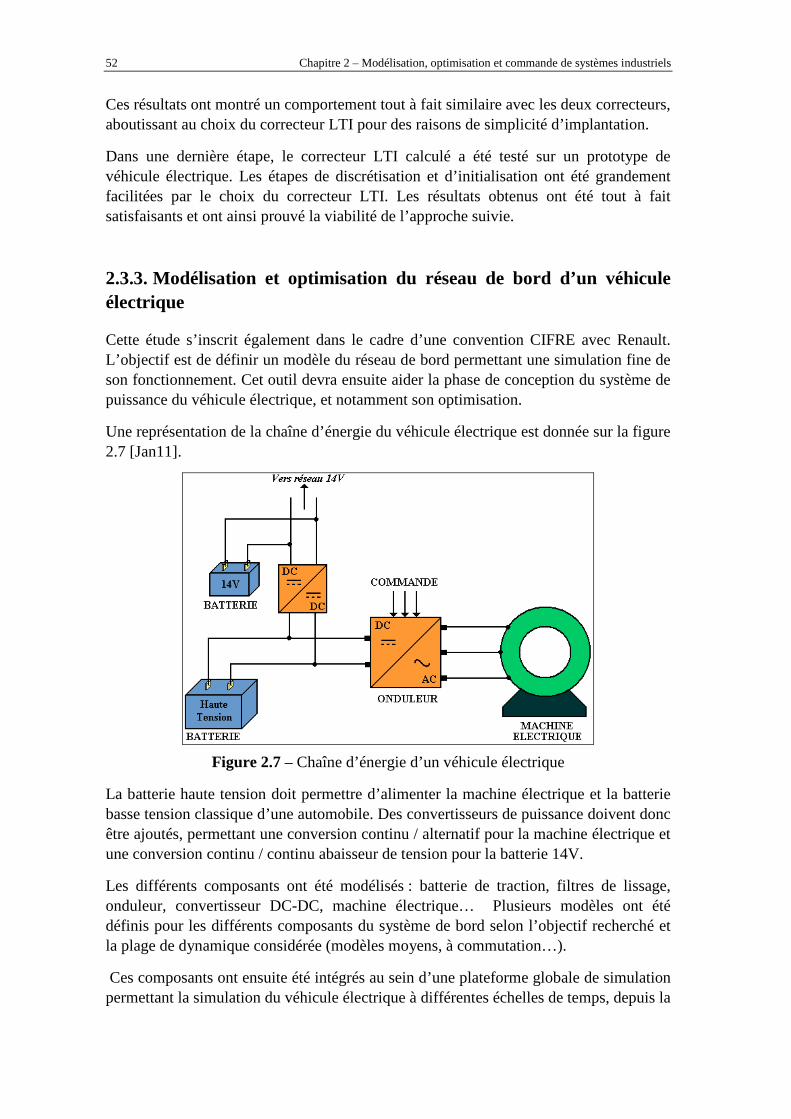
52 Chapitre 2 – Modélisation, optimisation et commande de systèmes industriels
Ces résultats ont montré un comportement tout à fait similaire avec les deux correcteurs, aboutissant au choix du correcteur LTI pour des raisons de simplicité d’implantation.
Dans une dernière étape, le correcteur LTI calculé a été testé sur un prototype de véhicule électrique. Les étapes de discrétisation et d’initialisation ont été grandement facilitées par le choix du correcteur LTI. Les résultats obtenus ont été tout à fait satisfaisants et ont ainsi prouvé la viabilité de l’approche suivie.
2.3.3. Modélisation et optimisation du réseau de bord d’un véhicule électrique
Cette étude s’inscrit également dans le cadre d’une convention CIFRE avec Renault. L’objectif est de définir un modèle du réseau de bord permettant une simulation fine de son fonctionnement. Cet outil devra ensuite aider la phase de conception du système de puissance du véhicule électrique, et notamment son optimisation.
Une représentation de la chaîne d’énergie du véhicule électrique est donnée sur la figure 2.7 [Jan11].
Figure 2.7 – Chaîne d’énergie d’un véhicule électrique
La batterie haute tension doit permettre d’alimenter la machine électrique et la batterie basse tension classique d’une automobile. Des convertisseurs de puissance doivent donc être ajoutés, permettant une conversion continu / alternatif pour la machine électrique et une conversion continu / continu abaisseur de tension pour la batterie 14V.
Les différents composants ont été modélisés : batterie de traction, filtres de lissage, onduleur, convertisseur DC-DC, machine électrique… Plusieurs modèles ont été définis pour les différents composants du système de bord selon l’objectif recherché et la plage de dynamique considérée (modèles moyens, à commutation…).
Ces composants ont ensuite été intégrés au sein d’une plateforme globale de simulation permettant la simulation du véhicule électrique à différentes échelles de temps, depuis la

Chapitre 2 – Modélisation, optimisation et commande de systèmes industriels 53
simulation des transitoires rapides jusqu’à la simulation de cycles de roulage typiques… Un effort important à été porté sur la possibilité de renseigner et recaler les paramètres de ces modèles à partir des données disponibles.
Face à la complexité du modèle à définir en termes de nombre de composants, d’interconnexions de sous systèmes et d’entrées / sorties, une réflexion poussée a dû être menée pour définir la causalité des modèles de chaque constituant. Cette réflexion a été facilitée par l’utilisation de méthodologies de modélisation particulières telles que :
- les Bond Graphs [Dau99], [Dau00], [Gan03], [RA06] ;
- la Représentation Energétique Macroscopique (REM) [Bou03].
Concernant les critères d’optimisation, il est évident que l’autonomie du véhicule est la préoccupation première. Cependant, cette amélioration de l’autonomie ne doit pas se faire au détriment des performances dynamiques du véhicule. L’optimisation d’un véhicule électrique est donc par nature un problème d’optimisation multiobjectifs.
Dans un premier temps, une optimisation globale du système a été effectuée en utilisant des modèles rapides (caractéristiques statiques, modèles moyens…), et des profils de roulage classiques (cycle NEDC par exemple) [JVP10]. Pour ce faire, une réflexion importante a été menée afin de déterminer les paramètres les plus influents sur l’autonomie (vitesse du véhicule, masse, pente de la route…). Cette optimisation globale a permis entre autres de modifier l’architecture représentée sur la figure 2.7 pour inclure un convertisseur de tension continu / continu entre la batterie et le rotor de la machine électrique.
Dans un deuxième temps, des optimisations locales (au sens géographique du terme) ont été conduites pour le pilotage des différents organes dimensionnés à l’étape précédente. Un premier axe d’optimisation concerne le pilotage de la machine électrique. Nous avons eu recours à la commande vectorielle de la machine [Mul04]. Trois stratégies de pilotage ont été définies [JVB09], permettant de déterminer les consignes de courant fqd iii ,, dans le domaine de Park :
• Stratégie à maximum de couple, privilégiant les performances dynamiques ;
• Stratégie à minimum de pertes, privilégiant l’autonomie ;
• Stratégie hybride, mixant les deux approches précédentes.
Les problèmes éventuels dus à une saturation de la tension batterie (en fonction de l’état de charge notamment), et à une méconnaissance des pertes ont été pris en compte afin d’obtenir une loi de commande robuste. Enfin, le réglage des correcteurs PI des boucles de courant a été effectué.
Un deuxième axe d’optimisation a concerné l’onduleur de tension. Le but est de déterminer les tensions statoriques de référence. Pour ce faire, une étude a été menée pour optimiser les paramètres de la MLI3, et notamment le découpage de la période
3 Modulation à Largeur d’Impulsion
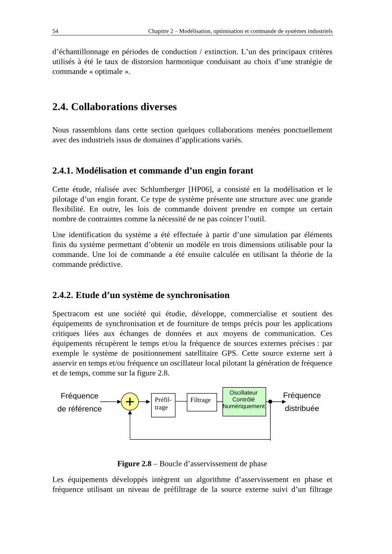
54 Chapitre 2 – Modélisation, optimisation et commande de systèmes industriels
d’échantillonnage en périodes de conduction / extinction. L’un des principaux critères utilisés à été le taux de distorsion harmonique conduisant au choix d’une stratégie de commande « optimale ».
2.4. Collaborations diverses
Nous rassemblons dans cette section quelques collaborations menées ponctuellement avec des industriels issus de domaines d’applications variés.
2.4.1. Modélisation et commande d’un engin forant
Cette étude, réalisée avec Schlumberger [HP06], a consisté en la modélisation et le pilotage d’un engin forant. Ce type de système présente une structure avec une grande flexibilité. En outre, les lois de commande doivent prendre en compte un certain nombre de contraintes comme la nécessité de ne pas coincer l’outil.
Une identification du système a été effectuée à partir d’une simulation par éléments finis du système permettant d’obtenir un modèle en trois dimensions utilisable pour la commande. Une loi de commande a été ensuite calculée en utilisant la théorie de la commande prédictive.
2.4.2. Etude d’un système de synchronisation
Spectracom est une société qui étudie, développe, commercialise et soutient des équipements de synchronisation et de fourniture de temps précis pour les applications critiques liées aux échanges de données et aux moyens de communication. Ces équipements récupèrent le temps et/ou la fréquence de sources externes précises : par exemple le système de positionnement satellitaire GPS. Cette source externe sert à asservir en temps et/ou fréquence un oscillateur local pilotant la génération de fréquence et de temps, comme sur la figure 2.8.
Figure 2.8 – Boucle d’asservissement de phase
Les équipements développés intègrent un algorithme d’asservissement en phase et fréquence utilisant un niveau de préfiltrage de la source externe suivi d’un filtrage
Fréquence
de référence
Fréquence
distribuée + Oscillateur Contrôlé
Numériquement Préfil-trage
Filtrage

Chapitre 2 – Modélisation, optimisation et commande de systèmes industriels 55
adaptatif de Kalman. Cet asservissement améliore d’un facteur 1000 la stabilité à long terme de la source de fréquence locale.
L’objectif de cette étude [RV10] était de construire un modèle simulant de manière réaliste le comportement de l’ensemble du filtrage existant puis d’optimiser le comportement de ce filtrage pour la « stabilité » à moyen terme (de 100s à 2h).
2.4.3. Etude d’un système d’estimation d’attitude
L’étude proposée [GM10] fait partie d’un projet plus global consistant à développer un système automatique gérant la sécurité de tir sur un terrain d’essai militaire. Les données analysées sont nombreuses (mesure de vent, de vitesse, de position) et permettent de fournir une autorisation de tir pour un char.
Afin de prévoir au mieux la position de l’impact d’un obus, il est nécessaire de connaitre très précisément l’orientation du tube de tir dans l’espace. L’objectif est ainsi de développer un système de mesure permettant de donner avec une grande précision l’attitude du tube.
Une première phase de l’étude a consisté en un recensement des technologies disponibles sur le marché (centrale inertielle, magnétomètre, gyromètre…) en les comparant en termes de temps de réponse, de précision de la mesure et de nécessité de recalage de la mesure. Les capteurs disponibles ne permettant pas de satisfaire toutes les contraintes du cahier des charges, nous avons donc, dans une deuxième phase, proposé une architecture du système permettant d’atteindre tous les objectifs.
Tout d’abord, une séparation des mesures est effectuée : attitude du châssis par rapport au repère terrestre, puis attitude du canon par rapport au châssis. Pour la première étape, des mesures issues de gyromètres sont recalées à l’aide d’un filtre de Kalman à partir de mesures fournies à une cadence plus faible par une centrale inertielle. Pour la deuxième étape, l’utilisation de radars hyperfréquences et des mesures fournies par le moteur permettant la rotation de la tourelle permet d’obtenir des mesures des angles relatifs entre le canon et le châssis. Enfin, à partir de toutes ces mesures, un deuxième filtre de Kalman permet d’estimer l’attitude du canon par rapport au repère terrestre.
2.5. Conclusions : bilan méthodologique
Nous avons présenté ici un rapide bilan des activités menées en collaboration avec des industriels. Il est relativement délicat de synthétiser ces travaux dans la mesure où il s’agit d’applications diverses ayant chacune leur spécificité. Cependant, il ressort un certain nombre de points communs qui méritent d’être mis en avant.
Il s’agit généralement de formaliser en un problème d’automatique les problématiques de commande apportées par les industriels. Dans cette optique, il s’agit de :

56 Chapitre 2 – Modélisation, optimisation et commande de systèmes industriels
• S’imprégner du domaine d’application afin d’en saisir les spécificités. Le calcul d’une commande, et encore plus la définition d’un problème d’optimisation, suppose une bonne connaissance des contraintes à respecter.
• Modéliser le système sous une forme adaptée au but recherché (simulation, optimisation, commande…). On retrouve toujours le compromis entre la représentativité du modèle et les temps de calcul nécessaires à sa simulation.
• Calculer une loi de commande en utilisant une méthode adaptée à la forme du problème et aux objectifs à atteindre.
Le point clé est assurément le deuxième, à savoir la détermination d’un ou plusieurs modèle(s) adapté(s) du système. En effet, il est très rare qu’une collaboration industrielle serve de cadre au développement d’une nouvelle méthode de commande ou d’un nouvel algorithme d’optimisation. Il s’agit généralement d’appliquer une méthode existante à un problème concret. Cette approche ne doit pas être considérée comme réductrice. En effet, elle suppose une bonne connaissance des outils existants afin de déterminer lequel pourra être utilisé. Elle nécessité également un travail important de reformulation du problème initial. Finalement, les travaux effectués constituent généralement une résolution exacte (le calcul d’une commande prédictive par résolution d’équations diophantiennes fournit la solution optimale au problème posé) d’un problème approché (les reformulations du problème initial se sont traduites par des simplifications ou des relaxations).
A ce stade un certain nombre de nouvelles problématiques apparaissent :
• La détermination d’un modèle adapté (sous entendu suffisamment simple mais représentatif) à une résolution par des méthodes classiques est parfois difficile, notamment à cause du grand nombre de variables et d’équations à prendre en compte ;
• La reformulation du problème entraîne souvent une relaxation des contraintes (certaines contraintes ne peuvent être reformulées de manière adéquate par exemple). Il est alors nécessaire de vérifier a posteriori que toutes les contraintes sont satisfaites. Cette vérification peut entraîner une alternance plus ou moins longue de phases de synthèse et d’analyse de la solution souvent consommatrice de temps ;
• L’objectif industriel peut être non seulement de satisfaire un cahier des charges mais en plus d’optimiser les performances du système. Cela conduit à optimiser les paramètres de réglage, rendant le problème d’optimisation sous-jacent extrêmement difficile à résoudre.
C’est pour toutes ces raisons qu’un deuxième volet des activités de recherche, plus théorique, est consacré à l’utilisation d’algorithmes d’optimisation stochastiques, les métaheuristiques. Cet aspect sera abordé au chapitre suivant.

Chapitre 3
Développement de méthodes génériques pour
l’Automatique fondées sur les métaheuristiques
3.1. Introduction ........................................................................................................ 59
3.2. Identification de systèmes .................................................................................. 60
3.2.1. Position du problème et état de l’art .............................................................. 60
3.2.2. Méthodologie proposée .................................................................................. 61
3.3. Optimisation de correcteurs PID ...................................................................... 66
3.3.1. Position du problème ..................................................................................... 66
3.3.2. Méthodologie proposée .................................................................................. 70
3.3.3. Optimisation multiobjectif ............................................................................. 74
3.4. Synthèse H∞∞∞∞ ......................................................................................................... 77
3.4.1. Optimisation des filtres de pondération ......................................................... 77
3.4.2. Synthèse H∞ d’ordre réduit ............................................................................ 84
3.5. Conclusions ......................................................................................................... 89

58 Chapitre 3 – Méthodes génériques pour l’Automatique

Chapitre 3 – Méthodes génériques pour l’Automatique 59
3.1. Introduction
Nous présentons dans ce chapitre un certain nombre de méthodologies qui ont été développées pour répondre à des problématiques d’automatique et fondées sur l’optimisation.
Lorsque l’on parcourt brièvement l’histoire de l’Automatique, on s’aperçoit très rapidement que l’optimisation a souvent été à la base des méthodes utilisées. Nous pouvons ainsi citer par exemple les méthodes de synthèse linéaire quadratique ou LQ [KS72] dans les années 70. Plus récemment sont apparues les méthodes de synthèses H2/H¶ ou H¶/H¶ [KDG96], pour lesquelles des méthodes de résolutions basées sur l’utilisation des inégalités matricielles affines (LMI) ont été développées, ou encore la paramétrisation de Youla-Kucera [FD87]. Parallèlement, la commande prédictive [CMT87], [Mac02] est apparue et constitue là encore une approche de commande optimale pondérant le suivi de référence et l’énergie de commande.
Ces différentes approches sont généralement fondées sur une reformulation convexe des problèmes d’optimisation pour laquelle des méthodes de résolution exactes et efficaces existent. C’est ainsi le cas des approches utilisant des modèles linéarisés du problème traité et des formulations quadratiques des critères. Si cette approche est tout à fait adaptée dans de nombreux cas, elle trouve un certain nombre de limites :
• Le travail de reformulation peut ne pas être évident. Ainsi, il est parfois délicat de transcrire les contraintes du cahier des charges en contraintes effectivement exploitables pour la synthèse. C’est typiquement le cas de la synthèse H∞, où les spécifications doivent être traduites en gabarits fréquentiels sur la boucle fermée. Cette nécessité de reformulation entraîne souvent le recours à de nombreux allers-retours entre synthèse et analyse pour vérifier a posteriori que les contraintes non prises en compte dans le formalisme utilisé sont satisfaites. De plus, elle rend l’utilisation des méthodes avancées délicate pour un non spécialiste qui ne saura pas faire facilement ce type de modification.
• Les différentes reformulations entraînent généralement des approximations par rapport au problème initial. En conséquence, même si les problèmes obtenus sont solubles de manière exacte, la solution obtenue n’est pas optimale au sens du problème initial.
• Les méthodes développées par ces approches permettent d’obtenir une loi de commande lorsque les paramètres de réglage sont fixés (exemple : choix des filtres de pondération dans le cas de la synthèse H∞). Il peut être intéressant non seulement de calculer une loi de commande, mais de l’optimiser. Dans ce cas les variables d’optimisation sont finalement les paramètres de réglage. Cette surcouche d’optimisation aborde ainsi des problèmes d’optimisation qui ne sont plus du tout convexes et pour lesquels les fonctions de coûts et de contraintes n’ont généralement pas d’expression analytique.

60 Chapitre 3 – Méthodes génériques pour l’Automatique
Des techniques d’optimisation non convexe ont plus récemment vu le jour pour traiter le problème initial. Des méthodes d’optimisation permettant de résoudre des problèmes d’optimisation non différentiables ont été utilisées, comme celles fondées sur le ε sous différentiel de Clarke [LF05]. Ces méthodes d’optimisation restent des méthodes d’optimisation locales, appartenant à la classe des méthodes de descente. Dans le domaine de la commande H∞, des solveurs existent désormais pour synthétiser des correcteurs d’ordre réduit (solveur HIFOO, [BHL06]) et / ou structurés (solveur ‘hinfstruct’ de Matlab, [SAN09], [ANS09]). Ces nouvelles méthodes fournissent des solutions dépendant fortement du point initial.
Les travaux que nous présentons ici se basent énormément sur l’utilisation d’une classe de méthodes d’optimisation stochastique, les métaheuristiques. Ces méthodes possèdent en effet l’avantage de ne requérir aucun calcul de gradient et ne préjugent ainsi pas de la structure mathématique des fonctions objectif et de contrainte. Elles sont donc un parfait candidat à la résolution des problèmes d’optimisation rencontrés en Automatique. L’inconvénient principal de ces méthodes est la quasi absence de garantie d’optimalité locale de la solution (les rares théorèmes de convergence sont des preuves de convergence en probabilité). Cet inconvénient a eu pour conséquence que ces méthodes ont été très peu utilisées en Automatique. Citons tout de même quelques exemples d’utilisation [ZLQ05], [MSK09].
Avant de présenter les différentes approches que nous avons développées, terminons cette introduction par deux arguments en faveur de l’utilisation de ces méthodes :
• Si aucune garantie d’optimalité ne peut être énoncée avec ces méthodes, en toute rigueur aucune garantie ne peut non plus être énoncée (vis-à-vis du problème initial) lorsque l’on utilise un algorithme exact sur un problème approché ;
• Il est toujours possible de récupérer la garantie d’optimalité locale en rajoutant une étape de post traitement à partir de la solution trouvée par la métaheuristique.
3.2. Identification de systèmes
3.2.1. Position du problème et état de l’art
La modélisation d’un système est bien sûr une étape fondamentale dans la conception d’une loi de commande. Que l’on parte d’un modèle de connaissance issu des lois de la physique, ou bien que l’on considère un modèle de comportement, il s’agit généralement d’identifier des paramètres. Dans de tels cas, une approche souvent utilisée est constituée par les moindres carrés [BW88]. Le problème d’optimisation sous-jacent est généralement non linéaire, et doit être résolu avec des méthodes ad’ hoc.
Nous nous intéressons ici à un problème plus complexe où non seulement les paramètres du modèle doivent être trouvés mais également sa structure. On parle alors de « régression symbolique ». Des techniques à base de réseaux de neurones peuvent

Chapitre 3 – Méthodes génériques pour l’Automatique 61
être utilisées [CBG90], [SS92]. Cependant, l’expression analytique qui en résulte est souvent très compliquée et ne peut être employée à des fins de commande. Nous cherchons ici des expressions mathématiques relativement simples. C’est pourquoi ce type de méthodes est plus répandu dans le domaine de l’apprentissage et de la classification [Zha00].
Plus récemment, les algorithmes génétiques ont été largement utilisés pour résoudre ce problème [DSW03], [GML98], [Hoa01], [MAS05], [Rai98], [SGD98], [WAW04]. Partant de la représentation sous forme d’arbre des fonctions mathématiques, des opérateurs de croisement et de mutation peuvent être créés, permettant la recherche d’expressions mathématiques. Cependant, il reste délicat avec ce type de méthode de rajouter de l’information a priori pour guider la recherche. Nous proposons ici de résoudre le problème en utilisant un algorithme de colonie de fourmis. Un tel algorithme a déjà été utilisé pour résoudre des problèmes d’approximation. Ainsi dans [BC02], [BCW02] l’algorithme est-il utilisé pour rechercher un programme approximant une fonction à partir d’un ensemble d’instructions. Dans [Yin03] un algorithme de colonie de fourmis est utilisé pour trouver une approximation d’une surface. Dans [GWJ04], l’algorithme est employé pour la résolution du problème de régression symbolique mais avec peu de succès.
3.2.2. Méthodologie proposée
3.2.2.1. Modélisation du problème
Nous considérons ici qu’une fonction )(xfy = doit être identifiée à partir de N points de mesure Niyx ii ,...,1),,( = . Nous recherchons ici non seulement les paramètres qui définissent la fonction f mais également son expression générale. Le problème peut alors s’écrire sous la forme du problème d’optimisation suivant :
∑=
−N
iii
fxfy
1
2))((min (Eq. 3.1)
Nous utilisons ici la représentation des fonctions sous forme d’arbre. En effet, toute fonction est composée d’opérateurs binaires (le ‘+’ par exemple) et d’opérateurs unaires (le ‘cos’ par exemple). Ainsi, la fonction )exp()3sin()( xxxf ×+= peut-elle se représenter sous la forme de l’arbre donné sur la figure 3.1.
Dans un deuxième temps, nous reformulons cet arbre sous forme d’arbre binaire complet en considérons qu’un opérateur unaire est un opérateur ayant un fils droit nul, ce que nous noterons par le symbole ∅ . Ainsi, l’arbre de la figure 3.1 devient celui de la figure 3.2.

62 Chapitre 3 – Méthodes génériques pour l’Automatique
Figure 3.1 – Représentation sous forme d’arbre de la fonction )exp()3sin()( xxxf ×+= .
Figure 3.2 – Représentation sous forme d’arbre binaire complet de la fonction )exp()3sin()( xxxf ×+= .
Les avantages procurés par cette représentation binaire complète sont :
• pour une profondeur de l’arbre p donnée, le nombre de nœuds est fixe et égal à 12 −p ;
• en numérotant les nœuds en largeur d’abord, les fils du nœud i sont les nœuds i2 et 12 +i .
Nous nous donnons maintenant un ensemble de symboles Ω autorisés, à partir desquels l’expression algébrique de la fonction pourra être formulée. Dans notre cas, nous choisissons par exemple :
×−+∅=Ω /,,,exp,cos,sin,,,,9,8,7,6,5,4,3,2,1 x (Eq. 3.2)
Dès lors, le problème (3.1) peut se reformuler, pour une profondeur p donnée par :
12,,1,.
))((min1
2,,
,, 121
121
−=Ω∈
−∑= −
−
pi
N
iii
ics
xfyp
p
K
K
K
θ
θθθθ (Eq. 3.3)
×
sin exp
x +
x 3
×
sin
x
+ x
exp
3
∅ ∅
∅ ∅ ∅ ∅ ∅ ∅

Chapitre 3 – Méthodes génériques pour l’Automatique 63
où 121 ,,
−pf θθ K
correspond à la fonction représentée sous forme d’arbre binaire complet
par les symboles 121 ,, −pθθ K . A ce problème d’optimisation doivent être ajoutées de
nombreuses contraintes permettant de ne créer que des fonctions viables. Ainsi par exemple si au nœud i on attribue le symbole cos=iθ , alors on devra attribuer au nœud
12 +i le symbole ∅=+12iθ , soit finalement :
∅=⇒= +12cos ii θθ (Eq. 3.4)
Ce problème d’optimisation est un problème d’optimisation combinatoire, mais dont l’expression de la fonction coût est non analytique. Dans la mesure où il s’agit d’une suite de décisions à prendre, nous proposons de le résoudre en utilisant un algorithme de colonie de fourmis.
3.2.2.2. Optimisation par colonie de fourmis
L’algorithme de colonie de fourmis permet de proposer un ensemble de solutions entières potentielles vérifiant les contraintes. Cet algorithme a été introduit par Marco Dorigo, et al. [DG96], [DMC96], [DBT00], [DS01]. Les algorithmes de colonie de fourmis reposent sur une analogie avec le comportement social de ces organismes. Le phénomène principal est le dépôt de phéromone sur le sol par les fourmis. Ce dépôt permet à une fourmi d’influencer les choix de ces congénères. Ainsi, plus un chemin est riche en phéromone et plus les fourmis auront tendance à l’emprunter. Ce processus s’apparente ainsi à une contreréaction positive.
L’observation de ce comportement a permis la définition d’algorithmes d’optimisation dont les premières applications ont été des problèmes de parcours de graphe. Considérons par exemple le problème ultra classique du voyageur de commerce tel que représenté sur la figure 3.3 [DM97]. Nous disposons ainsi d’un ensemble de nœuds (dans le cas du voyageur de commerce, il s’agit de villes) et d’arcs (ou de transitions) possibles entre ces nœuds. A chaque transition d’un nœud i à un nœud j , on associe un coût de transition ijd (dans le cas du voyageur de commerce, il s’agit de la distance entre ces nœuds). Le but est de passer dans toutes les villes une et une seule fois en minimisant la distance totale parcourue.
Pour résoudre ces problèmes, nous considérons que des « fourmis » parcourent ce graphe. Considérons ainsi une population de F fourmis. A l’itération t de l’algorithme, chaque fourmi f effectue un parcours. Lorsqu’elle arrive à un nœud i , il faut qu’elle choisisse sa prochaine transition. Ce choix peut se faire selon la probabilité suivante :
( ) ( ) ( )( )
( )∑
∈
=
iJmimim
ijijfi
f
t
tjp βα
βα
τη
τη
(Eq. 3.5)

64 Chapitre 3 – Méthodes génériques pour l’Automatique
Figure 3.3 – Problème du voyageur de commerce
Dans cette équation :
• ( )tijτ est la quantité de phéromone déposée sur l’arc ij à l’itération t par les fourmis des itérations précédentes ;
• ijη est la « désirabilité » intrinsèque d’opter pour le nœud j lorsqu’on est en i . Elle peut être égale par exemple à l’inverse du coût de la transition ijd1 : plus la transition entre deux nœuds est peu coûteuse, et plus l’envie de choisir cette transition est forte ;
• ( )iJ f est l’ensemble des nœuds accessibles depuis le nœud i pour la fourmi f : il s’agit de l’ensemble des nœuds atteignables depuis i , auquel on a retiré
tous les nœuds violant les contraintes (dans le cas du voyageur de commerce, il s’agit ainsi de tous les nœuds accessibles non précédemment visités). C’est cet ensemble, ( )iJ f , construit récursivement en même temps que chaque parcours, qui permet de gérer explicitement la faisabilité des solutions potentielles ;
• α et β sont deux coefficients permettant de pondérer la tendance panurgienne (« faire comme les autres fourmis ») et la vision court terme (« aller localement au plus court »).
Lorsque toutes les fourmis ont effectué leur parcours, ces parcours sont évalués et la phéromone est remise à jour selon l’équation suivante :
( ) ( ) ( ) ( )ttt ijijij ττρτ ∆+−=+ 11 (Eq. 3.6)
Le coefficient ρ est un facteur d’oubli, analogue à l’évaporation observée chez les fourmis réelles. En effet, du fait de la contre-réaction positive, le risque de converger rapidement vers un minimum local est important. Il est donc nécessaire d’ « oublier les erreurs du passé » et par exemple d’éventuelles mauvaises conditions initiales. La quantité de phéromone ajoutée sur l’arc ij , ( )tijτ∆ , dépend de la qualité des résultats de l’itération t . Elle est d’autant plus grande que les fourmis ayant opté pour l’arc ij
dij Noeud
Noeud

Chapitre 3 – Méthodes génériques pour l’Automatique 65
ont défini un parcours de faible coût. Plusieurs stratégies existent (seule(s) la ou les meilleure(s) fourmi(s) dépose(nt) de la phéromone sur les arcs parcourus, la quantité est bornée, la quantité est inversement proportionnelle à la longueur du meilleur trajet effectué…).
3.2.2.3. Adaptation au problème posé
Nous adaptons maintenant l’algorithme au problème de régression symbolique décrit au paragraphe 3.2.2.1. Supposons à l’itération k qu’une fourmi f ait choisi le symbole 1a au nœud i . Elle doit alors choisir des symboles pour les nœuds i2 et 12 +i . Pour ce faire, la probabilité qu’elle choisisse les symboles et 3a est donnée par :
( ) ( )( ) ( )∑
Ω∈→→
→→
→→
→→==→=
ω
βα
βα
ωτωη
τηθθ
)()(
)()()(
1,212
21,2212221
aa
aaaaaap
kiiii
kiiiiii
fk
( ) ( )( ) ( )∑ →→
→→=
=→=
Ω∈+→+→
+→+→
+ω
βα
βα
ωτωητη
θθ
)()(
)()(
1,12112
31,123112
312
1
aa
aaaa
a
ap
kiiii
kiiii
i
ifk
(Eq. 3.7)
Désormais, les valeurs de l’attractivité η dépendent non seulement de la transition mais également de la profondeur dans l’arbre i . Ceci permet de prendre en compte en particulier les contraintes terminales (si i2 correspond à un nœud du dernier niveau, le symbole correspondant doit être une constante ou une variable).
De manière générale, η peut permettre d’introduire de la connaissance a priori dans le système ou de favoriser les expressions simples.
3.2.2.4. Résultats obtenus
Nous choisissons les valeurs de paramètres suivantes :
• 1=α ;
• 2=β ;
• 2.0=ρ ;
• Nombre de fourmis : 10 ;
• Valeurs de η : 1 pour les transitions autorisées.
Nous utilisons un algorithme de colonie de fourmis de type MAX-MIN [SH97], [SH00]. Les résultats sont présentés dans les tableaux 3.1 et 3.2. Dans le premier tableau, la profondeur des arbres est fixée à 3. Les fonctions tests sont utilisées pour former les données et doivent être retrouvées par notre algorithme. Comme il s’agit d’un algorithme stochastique, il doit être validé de manière statistique. Ainsi, 100 tests sont faits pour chaque fonction. Un test est considéré comme un succès si le coût du
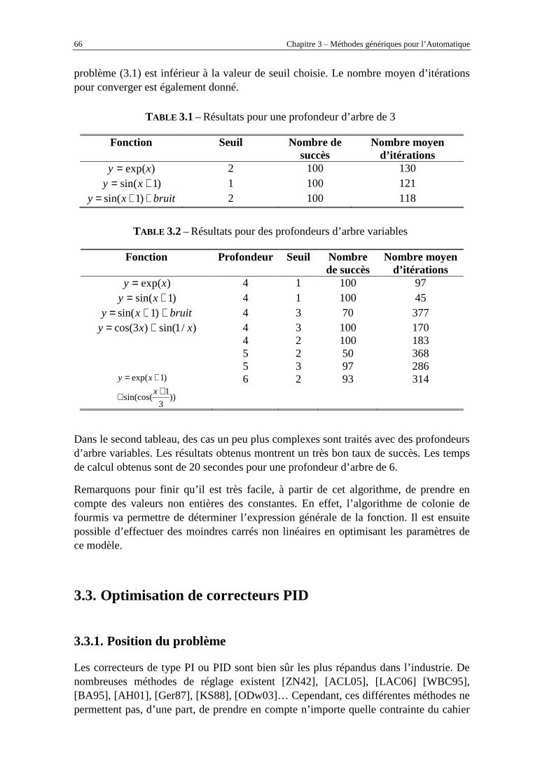
66 Chapitre 3 – Méthodes génériques pour l’Automatique
problème (3.1) est inférieur à la valeur de seuil choisie. Le nombre moyen d’itérations pour converger est également donné.
TABLE 3.1 – Résultats pour une profondeur d’arbre de 3
Fonction Seuil Nombre de succès
Nombre moyen d’itérations
)exp(xy = 2 100 130 )1sin( += xy 1 100 121
bruitxy ++= )1sin( 2 100 118
TABLE 3.2 – Résultats pour des profondeurs d’arbre variables
Fonction Profondeur Seuil Nombre de succès
Nombre moyen d’itérations
)exp(xy = 4 1 100 97 )1sin( += xy 4 1 100 45 bruitxy ++= )1sin( 4 3 70 377
)/1sin()3cos( xxy += 4 3 100 170 4 2 100 183 5 2 50 368 5 3 97 286
))3
1sin(cos(
)1exp(
++
+=x
xy
6 2 93 314
Dans le second tableau, des cas un peu plus complexes sont traités avec des profondeurs d’arbre variables. Les résultats obtenus montrent un très bon taux de succès. Les temps de calcul obtenus sont de 20 secondes pour une profondeur d’arbre de 6.
Remarquons pour finir qu’il est très facile, à partir de cet algorithme, de prendre en compte des valeurs non entières des constantes. En effet, l’algorithme de colonie de fourmis va permettre de déterminer l’expression générale de la fonction. Il est ensuite possible d’effectuer des moindres carrés non linéaires en optimisant les paramètres de ce modèle.
3.3. Optimisation de correcteurs PID
3.3.1. Position du problème
Les correcteurs de type PI ou PID sont bien sûr les plus répandus dans l’industrie. De nombreuses méthodes de réglage existent [ZN42], [ACL05], [LAC06] [WBC95], [BA95], [AH01], [Ger87], [KS88], [ODw03]… Cependant, ces différentes méthodes ne permettent pas, d’une part, de prendre en compte n’importe quelle contrainte du cahier

Chapitre 3 – Méthodes génériques pour l’Automatique 67
des charges, et, d’autre part, d’optimiser le réglage des paramètres du PID. Des techniques d’optimisation non lisse sont apparues plus récemment [ABN07], [BAN08] mais restent des techniques d’optimisation locale.
Considérons la boucle d’asservissement classique d’un système physique représentée sur la figure 3.4. Nous nous plaçons ici dans le cadre de systèmes linéaires, mais les résultats développés s’étendent sans problème aux systèmes non linéaires.
Système
)(sG ),( sθK
Correcteur + +
+ -
r u v y
d
ε
Figure 3.4 – Boucle d’asservissement
Le système G doit être piloté par le correcteur K , dont les paramètres de réglage sont notés θ , afin que la sortie y suive « au mieux » la référence r (l’écart ε doit rester faible), et ce malgré la présence de la perturbation d et en gardant une énergie de la commande u faible. A partir de ces notations, toutes les fonctions permettant de caractériser le comportement du système sont des fonctions des paramètres du correcteur. Ainsi, tout transfert de la boucle entre une entrée x et une sortie y quelconque est de la forme :
),()( θsHsT zx =→ (Eq. 3.8)
A partir de ces transferts, certaines spécifications peuvent se traduire en contraintes sur la représentation fréquentielle. Les critères les plus couramment utilisés dans le domaine fréquentiel sont les suivants, pour un correcteur de paramètres θ donné :
• Bande passante 0ω :
1
10
,1),(s.c
minarg)(1
ωωθω
ωθω
ε
ω
>∀<
=
→ jT y
(Eq. 3.9)
• Marge de phase φ∆ :
1),(avec
)180()),(arg()(
=°−−=∆
→
→
θωθωθφ
ε
ε
jT
jT
y
y (Eq. 3.10)
• Marge de module m∆ :
)1(),(min)( −−=∆ → θωθ εωjTm y (Eq. 3.11)
• Norme ∞H du système :

68 Chapitre 3 – Méthodes génériques pour l’Automatique
MiM
jTjTj
jT
i
yryrii
yr
deproprevaleurla)(et
)),(),((max),(avec
),(sup)(
èmeλ
θωθωλθωσ
θωσθω
→∗
→
∞→
=
=
(Eq. 3.12)
De manière plus générale, les spécifications fréquentielles se traduisent par des gabarits sur le module et la phase des différents transferts, par exemple :
Φ≤≤Φ
≤≤
→
→
)()),(arg()(
)(),()(
ωθωω
ωθωω
jjTj
jTjTjT
zx
zx (Eq. 3.13)
A titre d’exemple, la figure 3.5 montre le gabarit fréquentiel classique que doit respecter la boucle ouverte d’un transfert mono-variable : grands gains en basses fréquences afin d’assurer une bonne précision statique et dynamique, bande passante ω et marge de phase φ∆ suffisantes afin d’assurer respectivement une bonne rapidité et une bonne stabilité du système, faibles gains en hautes fréquences afin de filtrer les bruits.
ω
ω
dBG
φ
-180° φ∆
ω
Figure 3.5 – Gabarit fréquentiel classique pour la boucle ouverte d’un système mono-variable
De la même façon, les spécifications temporelles classiques des systèmes asservis telles que le dépassement en régime indiciel, le temps de réponse ou l’énergie de commande sont des fonctions des paramètres du correcteur :
• Dépassement en réponse indicielle %D :
+∞→
+∞→−
=
1
1
),(lim
),(lim),(
max)%(1
1
t
t
t ty
tyty
Dθ
θθθ (Eq. 3.14)
• Temps de réponse à %α :
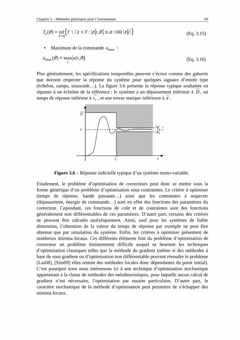
Chapitre 3 – Méthodes génériques pour l’Automatique 69
( ) ( ) trtTtTTT
e ⋅≤>∀=>
100/,:\inf)(0
αθεθ (Eq. 3.15)
• Maximum de la commande maxu :
),(max)(max θθ tuut
= (Eq. 3.16)
Plus généralement, les spécifications temporelles peuvent s’écrire comme des gabarits que doivent respecter la réponse du système pour quelques signaux d’entrée type (échelon, rampe, sinusoïde…). La figure 3.6 présente la réponse typique souhaitée en réponse à un échelon de la référence : le système a un dépassement inférieur à D , un temps de réponse inférieur à rt , et une erreur statique inférieure à ε .
1
t
D
rt
ε±
Figure 3.6 – Réponse indicielle typique d’un système mono-variable.
Finalement, le problème d’optimisation de correcteurs peut donc se mettre sous la forme générique d’un problème d’optimisation sous contraintes. Le critère à optimiser (temps de réponse, bande passante…) ainsi que les contraintes à respecter (dépassement, énergie de commande…) sont en effet des fonctions des paramètres du correcteur. Cependant, ces fonctions de coût et de contraintes sont des fonctions généralement non différentiables de ces paramètres. D’autre part, certains des critères ne peuvent être calculés analytiquement. Ainsi, sauf pour les systèmes de faible dimension, l’obtention de la valeur du temps de réponse par exemple ne peut être obtenue que par simulation du système. Enfin, les critères à optimiser présentent de nombreux minima locaux. Ces différents éléments font du problème d’optimisation de correcteur un problème éminemment difficile auquel se heurtent les techniques d’optimisation classiques telles que la méthode du gradient (même si des méthodes à base de sous gradient ou d’optimisation non différentiable peuvent résoudre le problème [Las08], [Sim09] elles restent des méthodes locales donc dépendantes du point initial). C’est pourquoi nous nous intéressons ici à une technique d’optimisation stochastique appartenant à la classe de méthodes des métaheuristiques, pour laquelle aucun calcul de gradient n’est nécessaire, l’optimisation par essaim particulaire. D’autre part, le caractère stochastique de la méthode d’optimisation peut permettre de s’échapper des minima locaux.

70 Chapitre 3 – Méthodes génériques pour l’Automatique
3.3.2. Méthodologie proposée
3.3.2.1. Optimisation par essaim particulaire
L’optimisation par essaim particulaire est une méthode d’optimisation stochastique, appartenant à la classe de méthode des « métaheuristiques », qui a été introduite par Russel Eberhart et James Kennedy en 1995 [EK95]. Cette méthode est fondée sur le comportement social d’organismes vivants tels que les bancs de poissons et les groupes d’oiseaux.
Soit le problème d’optimisation générique :
)(min xfx χ∈
(Eq. 3.17)
On considère un ensemble de P particules dans l’espace de recherche χ . Chaque particule est animée d’un certain mouvement dans cet espace, et garde en mémoire la position où elle a obtenu sa meilleure performance au sens du critère à optimiser f . En outre, chaque particule est en communication avec un ensemble de particules « amies », appelé voisinage. Chaque particule connaît donc la meilleure position obtenue par l’une des particules de son voisinage. On note :
• kpx position de la particule p lors de l’itération k ;
• kpv vitesse de la particule p lors de l’itération k ;
• kpb position où la particule p a obtenu sa meilleure valeur, depuis le début de
l’algorithme, à l’itération k ;
• kpg position où les particules du voisinage de la particule p ont obtenu leur
meilleure valeur, depuis le début de l’algorithme, à l’itération k .
A chaque itération de l’algorithme, les différentes particules évoluent dans l’espace de recherche selon :
11
211 )()(.
++
+
+=
−⊗+−⊗+=kp
kp
kp
kp
kp
kp
kp
kp
kp
vxx
xgcxbcvwv (Eq. 3.18)
Dans ces équations :
• w est le facteur d’inertie ;
• ⊗ signifie multiplication terme à terme de deux vecteurs ;
• 1c (resp. 2c ) est un vecteur de longueur la dimension du problème d’optimisation, et dont les composantes sont tirées selon une distribution uniforme dans l’intervalle ],0[ 1c (resp. ],0[ 2c ).

Chapitre 3 – Méthodes génériques pour l’Automatique 71
L’algorithme réalise donc à chaque itération et pour chaque particule une combinaison aléatoire de trois tendances : continuer sur sa lancée, revenir sur ses pas, agir comme les autres particules.
De nombreuses variantes de l’algorithme existent dans la littérature. Ainsi, des variations dans l’écriture de la loi d’évolution (3.18) sont fréquemment proposées et analysées comme dans [ES00] ou [CS04] par exemple. De même, la topologie du voisinage des particules a été étudiée de manière intensive [Ken99]. Deux voisinages principaux peuvent être cités : le voisinage géographique et le voisinage social. Dans le voisinage géographique, les particules « amies » d’une particule donnée sont les particules situées les plus proches dans l’espace de recherche ; pour le voisinage social, les particules « amies » d’une particule donnée sont fixées une fois pour toutes, quelles que soient leurs positions au cours de l’algorithme. Le voisinage social est plus simple à mettre en œuvre et sera utilisé ici.
Le choix des paramètres de l’algorithme (taille de l’essaim, facteur d’inertie w , coefficients de pondération des tendances 1c et 2c , taille du voisinage des particules) est, comme pour toute méthode de type métaheuristique, un élément important qui a été abondamment étudié [SE98], [Tre03] par exemple. Cependant, la retouche d’un correcteur est souvent une problématique industrielle qui doit être faite sur site, en fonction des conditions courantes de production, par un technicien non nécessairement formé aux techniques d’optimisation sous-jacentes au réglage. D’autre part, on ne gagnerait rien à changer un problème de réglage de paramètres de correcteurs en un problème de réglage des paramètres de l’algorithme. Il est donc important d’utiliser une méthode d’optimisation générique. Nous utiliserons donc ici des réglages dits « standard », validés par James Kennedy et Maurice Clerc [KC06] :
• Taille de l’essaim : D+10 , où D est le nombre de variables d’optimisation du problème ;
• ))2ln(2/(1=w ;
• )2ln(5,021 +== cc .
3.3.2.2. Résultats obtenus
Dans cette section, nous présentons des résultats numériques obtenus en optimisant des correcteurs calculés pour une maquette de suspension magnétique. Cette maquette peut se représenter conformément à la figure 3.7.

72 Chapitre 3 – Méthodes génériques pour l’Automatique
E l e c t r o -a i m a n t
P e n d u l e
P o s i t i o n
x
électro aimant
i
z E
V z
+10V
-10V
v z z
0
l
Z
capteur de position
Figure 3.7 – Maquette de suspension magnétique.
Le schéma-bloc du système linéarisé autour du point de fonctionnement 0=z est donné sur la figure 3.8.
)()(
)(sC
sε
sU =
Correcteur
20
21
1
1)(
)(
ω
s
G
sI
sZ
−−=
Suspension
ε u
d
z1
zV Capteur
β
Actionneur
sτ
K
sU
sI I
+=
1)(
)( i cz
V +
+
+
-
Figure 3.8 – Schéma-bloc de la suspension magnétique.
Les valeurs numériques des paramètres du modèle sont les suivantes :
• V/A09,0=IK ;
• s10.5 4−=τ ;
• A/m011,0−=G ;
• s/rad9,390 =ω ;
• m/V4000=β .
Le correcteur utilisé est un correcteur Proportionnel-Intégral-Dérivé (PID) filtré, de fonction de transfert :
sTs
sT
sTKsC
fd
d
i +⋅
+++=
1
1
1
11)(
τ (Eq. 3.19)

Chapitre 3 – Méthodes génériques pour l’Automatique 73
Par convention, la constante de temps du filtrage de l’action dérivée est choisie telle que : 10/dd T=τ . Les paramètres du correcteur à optimiser sont donc
Tfdi TTTK ),,,(=θ .
Afin d’illustrer la variété des critères qui peuvent être optimisés par notre algorithme, nous cherchons désormais à trouver un correcteur satisfaisant le cahier des charges suivant :
• Maximum de commande délivré par le correcteur : V10)(max ≤tut
;
• Marge de module minimale : 5,0min =∆=∆ mm ;
• Temps de réponse minimal.
Nous introduisons les contraintes sous la forme de fonctions de pénalité. Finalement le critère optimisé peut s’écrire, )(sG étant la boucle ouverte corrigée :
( ) ( )
0)(
sinon
)5,0)1()(min()(
5,0)1()(minsi
0)(
sinon
)10))(max(exp()(
:10))(max(si
)100/5:\inf()(avec,
)()()(min
2
22
1
1
0
21
=
−−−⋅=
<−−=
−=
>
⋅≤>∀=
++
>
θ
ωαθ
ωθ
λθ
εθ
θθθ
ω
ω
θ
J
jGJ
jG
J
tuJ
tu
trtTtTJ
JJJ
t
t
T
(Eq. 3.20)
Notons que la contrainte sur la commande est une contrainte technique donc stricte. La pénalité choisie est proche d’une pénalité barrière. En ce qui concerne la pénalité sur la contrainte de marge de module, nous avons opté pour une pénalité quadratique, plus douce. En effet, la contrainte sur la marge de module est une contrainte plus souple, qui peut être légèrement violée.
Le tableau 3.3 présente des résultats statistiques de cette optimisation.
TABLE 3.3 – Résultats statistiques de l’optimisation de correcteur
Meilleur Pire cas Moyenne Ecart-type
30,8.10-3 s 39,7.10-3 s 31,4.10-3 s 1,1.10-3 s

74 Chapitre 3 – Méthodes génériques pour l’Automatique
Notons que le critère optimisé est un critère non partout différentiable. De plus, de nombreux minima locaux existent. Ainsi, un algorithme déterministe classique se trouve rapidement bloqué. A titre d’exemple, nous avons testé la méthode du simplexe de Nelder et Mead [NM64] à partir de chacun des points de chaque population initiale. Il n’a jamais été possible de trouver un correcteur aussi performant que ceux calculés par la méthode d’optimisation par essaim particulaire. D’autre part, un tel algorithme, initialisé par un correcteur non stabilisant ne peut pas toujours converger vers un correcteur stabilisant, au contraire de la méthode développée.
3.3.3. Optimisation multiobjectif
Plus récemment, nous avons proposé [IS10] d’étendre ces résultats en utilisant l’optimisation par essaim particulaire dans un contexte multiobjectif. Tout comme les algorithmes évolutionnaires [Coe99], [Jas04], l’algorithme d’optimisation par essaim particulaire est en effet un algorithme à base de population et donc tout à fait adapté à la résolution de ce type de problèmes [Ber01].
L’optimisation multi-objectifs consiste en la minimisation « simultanée » de k objectifs :
)(,),(min 1 xfxf kx
K (Eq. 3.21)
Une telle optimisation est réalisée au sens de la Pareto optimalité [EG00], [TMJ99]. Une solution x domine une autre solution y si :
)()(t.q.et)()(, yfxfjyfxfi
yx
jjii <∃≤∀⇔p
(Eq. 3.22)
Une solution est dite « Pareto optimale », si elle n’est dominée par aucune autre. La principale difficulté dans l’extension de l’algorithme d’optimisation particulaire au cas multi-objectifs réside dans la définition de « leaders » ou« guides » k
pkp gb , . Quelques
implémentations ont déjà été réalisées [RC06], [SRC06], [CEC05], [AEF05]. L’algorithme présenté a l’avantage de ne pas utiliser de mesure de distance dans l’espace des objectifs, mais uniquement le concept de dominance. Ceci permet de s’affranchir en partie des problèmes de sensibilité à la formulation des critères. En utilisant [AEF05], le guide local kpb suit l’équation d’évolution :
kp
kp
kp
kp
kp
kp
kp
kp
kp
kp
bb
xb
xbbxbx
=
=+
++
+++
1
11
111
sinon
alors
)et(ou)(Si pfpfp
(Eq. 3.23)

Chapitre 3 – Méthodes génériques pour l’Automatique 75
Où le symbole pf signifie qu’on ne peut pas comparer les deux solutions au sens de la dominance. La définition des leaders globaux k
pg passe par la définition d’une matrice d’archive A contenant à l’itération k toutes les solutions non dominées connues. Ainsi, à l’itération 1+k , toutes les particules 1+k
px qui ne sont dominées par aucune des solutions de l’archive sont incorporées à l’archive. En revanche, toute solution de l’archive dominée par l’une des particules de l’essaim sort de cette archive. A partir de cette archive, nous pouvons alors définir les ensembles suivants :
k
pkp
ka
kx
xaxX
xaaA
p
p
quetel
quetel
=
∈= A (Eq. 3.24)
Ainsi, kxA représente pour une solution potentielle x l’ensemble des éléments de
l’archive qui la dominent, et kaX représente, pour un élément a de l’archive,
l’ensemble des particules de l’essaim qu’elle domine. Dès lors, pour une particule kpx , le guide global choisi est :
=∈
∈∈=
sinon/éprobabilitlaavec,,A
Asi/éprobabilitlaavecA
ka
kp
kx
kp
kak
pXxxa
xXag
α
α (Eq. 3.25)
Où est le cardinal de kaX et α est choisi afin d’avoir la somme des probabilités
égale à 1. L’équation (3.25) s’interprète de la façon suivante : il est clair que les éléments de l’archive qui dominent une particule sont des candidats intéressants pour jouer le rôle de guide global. D’autre part, en choisissant une probabilité inversement proportionnelle à k
aX , on favorise les éléments de l’archive dominant peu de particules, espérant ainsi obtenir un front de Pareto plus large. Remarquons encore une fois que le passage à un algorithme multiobjectifs n’entraîne pas de paramètres de réglage. L’algorithme utilisé ici reste donc un algorithme sans paramètre ni reformulation. Nous choisissons ici de synthétiser un correcteur pour la suspension magnétique (section 3.3.2) en résolvant le problème d’optimisation multi-objectif suivant :
∫∫ ==
=
==5,0
02
25,0
02
1
21),,,(
)()(,)()(:avec
)(),(min
tt
TTTK
dttufdttf
fffdi
θεθ
θθθ
(Eq. 3.26)
en réponse à un échelon de consigne. Ces deux objectifs sont clairement contradictoires. Le simulateur prend en compte la saturation de la commande à V5± . La figure 3.9 présente le front de Pareto obtenu par l’algorithme d’optimisation par essaim particulaire multi-objectif ainsi que des réponses typiques obtenues pour les points du front (a) qui favorise le plus le critère 1, (b) qui favorise le plus le critère 2 et (c) qui réalise un compromis entre les deux. Les temps de calcul sont de 1 minute avec Matlab 2007b sur un Pentium 2,5 GHz.

76 Chapitre 3 – Méthodes génériques pour l’Automatique
Point a)
0 0.05 0.1 0.15 0.2 0.25 0.3 0.350
0.2
0.4
0.6
0.8
1
1.2
1.4
temps
Rép
onse
0 0.05 0.1 0.15 0.2 0.25 0.3 0.35-5
-4
-3
-2
-1
0
1
2
3
4
5
temps
com
man
de
Point b)
0 0.2 0.4 0.6 0.8 1 1.2 1.4 1.6 1.8 20
0.2
0.4
0.6
0.8
1
1.2
1.4
1.6
1.8
2
temps
Rép
onse
0 0.2 0.4 0.6 0.8 1 1.2 1.4 1.6 1.8 2-1
-0.5
0
0.5
1
1.5
2
2.5
3
3.5
4
temps
com
man
de
Point c)
0 0.1 0.2 0.3 0.4 0.5 0.6 0.7 0.80
0.2
0.4
0.6
0.8
1
1.2
1.4
0 0.1 0.2 0.3 0.4 0.5 0.6 0.7 0.8
-2
-1
0
1
2
3
4
5
Figure 3.9 – Résultats d’optimisation multiobjectif.
0 0.02 0.04 0.06 0.08 0.1 0.12 0.140.05
0.1
0.15
0.2
0.25
0.3
0.35
0.4
Erreur quadratique
Ene
rgie
de
com
man
de
a)
c) b)
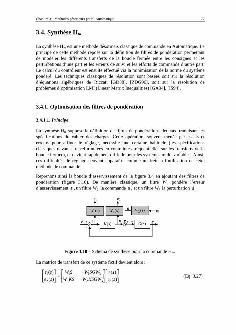
Chapitre 3 – Méthodes génériques pour l’Automatique 77
3.4. Synthèse H∞∞∞∞
La synthèse H¶ est une méthode désormais classique de commande en Automatique. Le principe de cette méthode repose sur la définition de filtres de pondération permettant de modeler les différents transferts de la boucle fermée entre les consignes et les perturbations d’une part et les erreurs de suivi et les efforts de commande d’autre part. Le calcul du contrôleur est ensuite effectué via la minimisation de la norme du système pondéré. Les techniques classiques de résolution sont basées soit sur la résolution d’équations algébriques de Riccati [GD88], [ZDG96], soit sur la résolution de problèmes d’optimisation LMI (Linear Matrix Inequalities) [GA94], [IS94].
3.4.1. Optimisation des filtres de pondération
3.4.1.1. Principe
La synthèse H∞ suppose la définition de filtres de pondération adéquats, traduisant les spécifications du cahier des charges. Cette opération, souvent menée par essais et erreurs pour affiner le réglage, nécessite une certaine habitude (les spécifications classiques devant être reformulées en contraintes fréquentielles sur les transferts de la boucle fermée), et devient rapidement difficile pour les systèmes multi-variables. Ainsi, ces difficultés de réglage peuvent apparaître comme un frein à l’utilisation de cette méthode de commande.
Reprenons ainsi la boucle d’asservissement de la figure 3.4 en ajoutant des filtres de pondération (figure 3.10). De manière classique, un filtre 1W pondère l’erreur d’asservissement ε , un filtre 2W la commande u , et un filtre 3W la perturbation d .
)(sG )(sK +
+ +
-
r ε u
d
v y
)(1 sW )(2 sW )(3 sW
1e 2e
3e
Figure 3.10 – Schéma de synthèse pour la commande H∞.
La matrice de transfert de ce système fictif devient alors :
−−
=
)(
)(
)(
)(
3322
311
2
1
se
sr
KSGWWKSW
SGWWSW
se
se (Eq. 3.27)

78 Chapitre 3 – Méthodes génériques pour l’Automatique
La solution du problème H¶ pour ce système, aboutissant à un correcteur K et une norme du transfert (3.27) égale à γ impose des contraintes aux différents transferts de la matrice de transfert. Par exemple, pour un système mono-variable :
≤
≤
≤
≤
∀⇒
≤
−−
∞
)()()(
)()()(
)()(
)()(
32
31
2
1
322
311
ωωγω
ωωγω
ωγω
ωγω
ω
γ
jWjWjKSG
jWjWjSG
jWjKS
jWjS
KSGWWKSW
SGWWSW
(Eq. 3.28)
Ainsi, la définition des filtres iW permet de modeler les différents transferts de la boucle fermée pour satisfaire le cahier des charges. La définition de ces filtres peut être difficile car le cahier des charges peut faire apparaître des spécifications temporelles sur la boucle fermée (temps de réponse, dépassement, énergie de commande, temps de rejet des perturbations…) et/ou des spécifications fréquentielles sur la boucle ouverte (bande passante, marge de phase…) qui doivent être traduites en gabarits fréquentiels sur la boucle fermée. Cette opération peut être délicate, notamment pour un système multi-variable.
Cependant, il est clair que tous les critères de performances, dont certains ont été rappelés dans la section 3.3 sont alors des fonctions des paramètres définissant les filtres de pondération. Nous proposons ainsi une nouvelle approche. L’idée est de reformuler le problème de réglage des filtres de pondération sous forme de problème d’optimisation. Les différentes spécifications sont alors explicitement prises en compte sous la forme de contraintes du problème d’optimisation, et ne nécessitent pas de reformulation.
3.4.1.2. Résultats obtenus
La méthode de réglage va être testée sur un système de chariot, piloté par un moteur à courant continu, et sur lequel est monté un pendule. Le système considéré est représenté sur la figure 3.11.

Chapitre 3 – Méthodes génériques pour l’Automatique 79
Moteur
Réducteur
Génératricetachymétrique
Potentiomètre
Potentiomètre
Charge
Chariot
u
i
ϕ xc
ω
Figure 3.11 – Système de pont roulant avec pendule.
Le système considéré peut être modélisé par les équations suivantes :
)()()()(
tutKtiRtd
tidL e =++ ω (Eq. 3.29a)
)()()()(
tiKtdtftd
tdJ e=++ ωω
(Eq. 3.29b)
)()(
tN
r
td
txd c ω= (Eq. 3.29c)
0)(sin)(cos2
2
2
2
=+++ φφαφφ gtd
d
td
dl
td
xd c (Eq. 3.29d)
Avec :
• )(ti : courant dans le moteur ;
• )(tu : tension aux bornes du moteur ;
• )(tω : vitesse de rotation du moteur ;
• )(txc : position du chariot ;
• )(tφ : angle du pendule ;
• )(td : perturbation de couple ;
• H0002,0=L : inductance du moteur ;
• Ω= 3,2R : résistance du moteur ;
• Nm/A0162,0=eK : constante électromagnétique ;
• 26kg.m10.5 −−=J : inertie du moteur ;
• N.m.s10.6 5−=f : coefficient de frottement ;

80 Chapitre 3 – Méthodes génériques pour l’Automatique
• m022,0=r : rayon de la poulie ;
• 17=N : facteur de réduction ;
• m275,0=l : longueur du pendule ;
• 1m.s3,0 −=α : coefficient de frottement du pendule ;
• 2m.s81,9 −=g : accélération de la pesanteur.
)(txc et )(tφ sont les grandeurs mesurées. Le cahier des charges est le suivant :
• En réponse à la consigne particulière de la figure 3.12 :
o Suivi sans dépassement ni erreur statique (une erreur de traînage est tolérée) ;
o Peu d’oscillation du pendule : rad01,0)( ≤tφ ;
o Efforts de commande faibles : V2)( ≤tu ;
o Bande passante supérieure à 1rad.s1 − .
o Marge de module supérieure à 0,5.
• En réponse à un échelon de couple perturbateur de Nm01,0)( =td :
o Influence sur la position du chariot : m01,0)( ≤txc ;
o Influence sur le pendule rad015,0)( ≤tφ ;
o Rejet de la perturbation.
0,4 m
0
0 4s
Figure 3.12 – Consigne de position appliquée au chariot.
Afin de résoudre le problème d’asservissement, nous choisissons de synthétiser un correcteur à 3 entrées (écart entre la consigne et la position, position du chariot et angle du pendule) conformément au schéma de synthèse de la figure 3.13. )(sG est le système obtenu en linéarisant les équations du système (3.23) autour du point 0=φ .

Chapitre 3 – Méthodes génériques pour l’Automatique 81
)(sG
)(sK
+ -
r ε u d
φ
)(1 sW )(2 sW )(3 sW
1e 2e
3e
cx
)(4 sW 4e
)(5 sW 5e
)(6 sW 6e
-
- +
+
Figure 3.13 – Schéma de synthèse à trois degrés de liberté.
Classiquement, l’influence des filtres est la suivante :
• 1W permet de régler le suivi de référence ;
• 2W permet de régler les efforts de commande ;
• 3W permet de régler le rejet de perturbation ;
• 4W pondère l’importance relative de la sortie position )(txc et de la sortie angle du pendule )(tφ ;
• 5W et 6W pondèrent l’influence des 3 mesures pour le calcul de la commande par )(sK . Ainsi augmenter ces deux filtres par exemple conduira la synthèse à considérer les deux mesures correspondantes comme très bruitées, et la synthèse conduira à un correcteur n’utilisant que la sortie position )(txc .
Nous choisissons les expressions suivantes pour les différents filtres de pondération :
s
sksW
2
111 1
1)(
ττ
++⋅= (Eq. 3.30a)
s
sksW
4
322 1
1)(
ττ
++⋅= (Eq. 3.30b)
33 )( ksW = , 44 )( ksW = , 55 )( ksW = , 66 )( ksW = (Eq. 3.30c)
Le problème d’optimisation peut donc s’écrire :
=
∞
6
5
3
4
2
1
,,,,,,,,
)(avec,)(min
4321
654321
e
e
e
r
sT
e
e
e
sTkkkkkk
ττττ
(Eq. 3.31)

82 Chapitre 3 – Méthodes génériques pour l’Automatique
Les différentes spécifications du cahier des charges sont des contraintes du problème d’optimisation. L’optimisation par essaim particulaire étant un algorithme d’optimisation pour des problèmes non contraints, des fonctions de pénalité sont ajoutées au critère. Ainsi, si l’on note )(),(),( tuttx rrcr φ les signaux obtenus en réponse à la consigne de la figure 3.12, )(),(),( tuttx ddcd φ les signaux obtenus en réponse à un échelon de perturbation de Nm01,0)( =td , la bande passante du système corrigé par
BPω et sa marge de module par m∆ , le critère à optimiser devient :
⋅+
−⋅+
−⋅+∆−⋅+
−⋅+
−⋅+
−⋅+∞
))(lim1000exp(
))01,0)(max(1000exp(
))015,0)(max(1000exp(
))5,0(1000exp(
))1(1000exp(
))2)(max(1000exp(
))01,0)(max(1000exp(
)(
min
4321
654321,,,
,,,,,
tx
tx
t
m
tu
t
sT
cdt
cdt
dt
BP
rt
rt
kkkkkk
φ
ω
φ
ττττ
(Eq. 3.32)
Les fonctions de pénalité choisies sont des fonctions très dures, proches de pénalité barrière. Un tel choix a été fait pour ne pas rajouter de paramètres de réglage dans le problème d’optimisation.
Remarquons que les différentes pénalités ne peuvent être calculées que par simulation, ce qui n’est pas un problème pour un algorithme tel que l’optimisation par essaim particulaire, qui suppose simplement d’être capable d’évaluer la fonction coût à optimiser.
La méthode d’optimisation a été implantée à l’aide de Matlab 2007b et Simulink 7.0 sur un Pentium IV, 2 GHz. La résolution du problème nécessite 15 minutes de calcul, pour un nombre d’itérations de l’algorithme fixé à 20. L’algorithme proposé est un algorithme stochastique. Dès lors, il est nécessaire d’exécuter plusieurs fois l’algorithme pour une même instance du problème afin d’obtenir des résultats statistiques sur la qualité des résultats et ainsi de valider l’approche proposée. 40 tests ont donc été effectués pour le problème (3.32), conduisant aux résultats du tableau 3.4.
Les résultats obtenus sont présentés dans les figures 3.14 (suivi de consigne), 3.15 (rejet de perturbation), et 3.16 (diagramme de Bode de la fonction de sensibilité). Les résultats présentés correspondent à une norme H¶ de 0,79 (norme obtenue pour le système corrigé par le correcteur moyen) pour le système de la figure 3.13. Les filtres correspondants sont :
00094.0
84.2332.0)(1 +
+=s
ssW
2.173
0866.02)(2 +
+⋅=s
ssW
01.0)(,1.0)(,10)(,0032.0)( 6543 ==== sWsWsWsW
(Eq. 3.33)

Chapitre 3 – Méthodes génériques pour l’Automatique 83
0 5 10 15 20 25-0.5
0
0.5
Pos
ition
(m
)
Reference
Position
0 5 10 15 20 25-0.01
0
0.01
Phi
(ra
d)
0 5 10 15 20 25-4
-2
0
2
u (V
)
Time (s)
Figure 3.14 – Suivi de consigne.
0 5 10 15 20 25-4
-2
0
2x 10
-3
Pos
ition
(m
)
0 5 10 15 20 25-5
0
5
10x 10
-3
Phi
(ra
d)
Figure 3.15 – Rejet de perturbation.
10-4
10-2
100
102
104
10-4
10-3
10-2
10-1
100
101
Sensitivity function
Figure 3.16 – Fonction de sensibilité.

84 Chapitre 3 – Méthodes génériques pour l’Automatique
TABLE 3.4 – Résultats de l’optimisation des filtres de pondération (norme H∞)
Meilleur cas Moyenne Pire cas
0,683 0,788 1,001
Le problème d’optimisation résolu est un problème très difficile avec de nombreux minima locaux, ce qui explique la relative disparité des résultats obtenus. De plus, nous nous sommes limités à 20 itérations de l’algorithme d’optimisation par essaim particulaire et une augmentation du nombre d’itérations conduit naturellement à une diminution de l’écart-type des résultats. Enfin, la population initiale est constituée de manière complètement aléatoire, afin d’explorer tout l’espace de recherche, mais induisant nécessairement une plus grande variété des résultats.
Néanmoins, les résultats demeurent très satisfaisants, avec à chaque fois le calcul d’un correcteur permettant de satisfaire le cahier des charges. Rappelons qu’aucune traduction de ce cahier des charges n’a été nécessaire pour prendre en compte les critères de performances demandés, exprimés sous forme de contraintes temporelles sur des réponses particulières de la boucle fermée et sous forme de contraintes fréquentielles sur la boucle ouverte. De plus, aucun réglage de paramètres n’est nécessaire.
3.4.2. Synthèse H∞∞∞∞ d’ordre réduit
3.4.2.1. Synthèse de correcteurs d’ordre réduit
Il est bien connu que la synthèse H∞ produit des correcteurs d’ordre élevés, généralement de l’ordre du modèle de synthèse (modèle du système plus filtres de pondération). Si l’on rajoute une contrainte sur l’ordre du système, le problème d’optimisation sous-jacent devient non convexe du fait de contraintes de rang sur des matrices. Le problème de synthèse H∞ d’ordre réduit se traduit alors sous forme de problème BMI (Bilinear Matrix Inequality).
Pour résoudre le problème, plusieurs approches existent :
• approximations convexes du problème, souvent obtenues à partir de considérations conservatives ;
• optimisation globale non linéaire, mais qui peuvent être très couteuses en temps de calcul ;
• optimisation locale, comme les solvers BMI. La solution dépend alors du point initial et il n’y a pas de garantie d’optimalité globale.
Ainsi, plusieurs heuristiques ont pu être développées : choix de pénalités barrières [DD93], [DD94], [Dav94] ; projection sur des sous-ensembles définis pour chacune des

Chapitre 3 – Méthodes génériques pour l’Automatique 85
contraintes [NN93], [BE93] ; résolutions alternées pour retrouver une suite de problèmes convexes [RI94], [IS95] ; complémentarité conique [EOA97].
Plus récemment, des méthodes fondées sur l’optimisation non différentiable sont apparues [AN06], [BHL06], [Bom07], [BNA07], [ANR08], [Sim09], [ARN11]. Ces travaux ont abouti à la création du solveur HIFOO et de la routine ‘hinfstruct’ de Matlab. Ces solveurs restent des optimisations locales. Les résultats peuvent donc dépendre fortement du ou des points initiaux.
Nous proposons ici une méthode d’optimisation globale fondée sur les essaims particulaires. L’avantage de cette méthode est le fait que nous pourrons intégrer non seulement la contrainte sur l’ordre du correcteur, mais également toutes les autres contraintes du cahier des charges.
Nous reprenons l’exemple du pont roulant traité dans la section 3.4.1, en conservant les filtres de pondération moyens obtenus. La synthèse du problème (à ordre plein) conduit alors à un ordre 6 pour le correcteur à trois degrés de liberté (4 pour le système, 1 pour
1W et 1 pour 2W ). Nous cherchons un correcteur d’ordre 2, de la forme :
T
ss
ssK
ss
ssK
ss
ssK
sK
++++++++
++++
=
)1)(1(
)1)(1(
)1)(1(
)1)(1(
)1)(1(
)1)(1(
)(
21
32313
21
22212
21
12111
ττττττττ
ττττ
(Eq. 3.34)
Le problème d’optimisation peut alors s’écrire, en conservant le cahier des charges et les notations de la section 3.4.1 :
∆−⋅+−⋅+
−⋅+
−⋅+
⋅+−⋅+
−⋅+⋅+
+∞→
∞
))5.0(1000exp())1(1000exp(
))05.0)(max(1000exp(
))01.0)(max(1000exp(
))(lim1000exp())2)(max(1000exp(
))05.0)(max(1000exp()1000exp(
)(
min
3231
2221
1211
21
321
,,,,
,,
m
t
tx
txtu
tD
sT
BP
dt
cdt
cdt
rt
rt
KKK
ω
φ
φ
ττττττττ
(Eq. 3.35)
Les résultats sont donnés dans le tableau 3.5. Les temps de calcul sont de l’ordre de 300 secondes (Pentium IV, 2GHz, Matlab R2007).
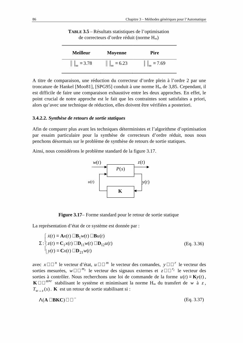
86 Chapitre 3 – Méthodes génériques pour l’Automatique
TABLE 3.5 – Résultats statistiques de l’optimisation de correcteurs d’ordre réduit (norme H∞)
Meilleur Moyenne Pire
78.3=∞ 23.6=∞
69.7=∞
A titre de comparaison, une réduction du correcteur d’ordre plein à l’ordre 2 par une troncature de Hankel [Moo81], [SPG95] conduit à une norme H∞ de 3,85. Cependant, il est difficile de faire une comparaison exhaustive entre les deux approches. En effet, le point crucial de notre approche est le fait que les contraintes sont satisfaites a priori, alors qu’avec une technique de réduction, elles doivent être vérifiées a posteriori.
3.4.2.2. Synthèse de retours de sortie statiques
Afin de comparer plus avant les techniques déterministes et l’algorithme d’optimisation par essaim particulaire pour la synthèse de correcteurs d’ordre réduit, nous nous penchons désormais sur le problème de synthèse de retours de sortie statiques.
Ainsi, nous considérons le problème standard de la figure 3.17.
Figure 3.17– Forme standard pour le retour de sortie statique
La représentation d’état de ce système est donnée par :
+=++=
++=Σ
)()()(
)()()()(
)()()()(
:
21
12111
1
twtxty
tutwtxtz
tutwtxtx
DC
DDC
BBA&
(Eq. 3.36)
avec nx ℜ∈ le vecteur d’état, mu ℜ∈ le vecteur des comandes, ry ℜ∈ le vecteur des sorties mesurées, 2mw ℜ∈ le vecteur des signaux externes et 2rz ℜ∈ le vecteur des sorties à contrôler. Nous recherchons une loi de commande de la forme )()( tytu K= ,
rm×ℜ∈K stabilisant le système et minimisant la norme H∞ du transfert de w à z , )(sT zw→ . K est un retour de sortie stabilisant si :
−ℜ∈+Λ )( BKCA (Eq. 3.37)
)(sP
K
)(tw )(tz
)(ty )(tu
Chapitre 3 – Méthodes génériques pour l’Automatique 87
Où )(MΛ est l’ensemble des parties réelles des valeurs propres de M .
Le problème d’optimisation s’écrit alors :
)()(.
min
tytucs
T zwrm
KK
=
∞→ℜ∈ × (Eq. 3.38)
La boucle pouvant être instable pour certaines valeurs de rm×ℜ∈K , le problème est reformulé en :
)(min KK
Jrm×ℜ∈
(Eq. 3.39)
avec :
∞→−= zwTJ /1)(K (Eq. 3.40)
si la boucle est stable, et :
))))(((Remax()( sTJ zw→= λK (Eq. 3.41)
sinon.
Le nombre de variables d’optimisation est ici rm× qui peut être rapidement important. Nous utilisons ici une version améliorée de l’algorithme d’optimisation par essaim particulaire [VE02], [Xin10] permettant de s’affranchir des risques de convergence prématurée de l’algorithme classique utilisée jusqu’à présent. L’idée générale est de perturber la meilleure solution courante afin de la forcer à continuer son exploration.
L’algorithme est comparé avec les résultats obtenus avec le solveur HIFOO [BHL06] (optimisation non lisse) et les résultats obtenus dans [AGP10] (utilisation de LMIs et d’algorithme stochastique du type « Hit and Run »). Pour ce faire, on teste la résolution sur la bibliothèque Compleib [Lei04] qui regroupe de nombreux exemples de systèmes issus de la littérature. Cette librairie est utilisée à des fins de benchmarks et de comparaison entre algorithmes [YC05]. Ces résultats sont présentés sur le tableau 3.6 [YS11]. Les résultats obtenus montrent que l’algorithme PSO utilisé, avec très peu de réglage (les valeurs des paramètres choisies sont directement tirées de [VE02] et n’ont pas été optimisées pour le problème posé), conduit à des résultats comparables aux meilleurs solveurs.

88 Chapitre 3 – Méthodes génériques pour l’Automatique
TABLE 3.6 –Synthèse de retours de sortie statiques H∞
Ex. n m r HIFOO Arz., et al. PSO
AC1 AC2 AC5 AC9 AC10 AC11 AC12 AC13 AC14 AC18
5 5 4 10 55 5 4 28 40 10
3 3 2 4 2 2 3 3 3 2
3 3 2 5 2 4 4 4 4 2
4.14 10-7
0.1115 669.56 1.0029
Inf 2.8335 0.3120 163.33
101.7203 12.6282
1.76 10-6
0.1115 661.7 1.0061
Inf 2.8375 0.6165
395.0404 319.31 10.6214
4.7 10-22
0.1115 665.09 1.098 Inf
2.8609 0.3134 167.36 101.96 27.18
HE1 HE3 HE4 HE5 HE6 HE7
4 8 8 4 20 20
2 4 4 2 4 4
1 6 6 2 6 6
0.1539 0.8061 22.8282 8.8952
192.3445 192.3885
0.1538 0.8291 22.8282 17.6061 401.7698 353.9425
0.1529 0.8399 23.43
10.0031 195.86 194.24
DIS2 DIS4 DIS5
3 6 4
2 4 2
2 6 2
1.0412 0.7394 1035.5
1.0244 0.7404 1030.82
1.0255 0.7863 1028
JE2 JE3
21 24
3 3
3 6
183.3512 5.0963
365.09 9.194
192.17 5.138
REA1 REA2 REA3
4 4 12
2 2 1
3 2 3
0.8694 1.1492 74.2513
0.8661 1.1482 74.2513
0.8738 1.1451 74.2513
WEC1 10 3 4 4.0502 4.1055 6.4843 BDT2 82 4 4 0.6471 2.90 1.0345 CSE 60 2 30 0.0201 0.02 0.0200 PAS 5 1 3 32.2258 0.0087 0.0571 TF1 TF2 TF3
7 7 7
2 2 2
4 3 3
0.3736 5200
0.4567
0.3799 5200
0.3264
0.4038 5200
0.5829 NN1 NN2 NN5 NN6 NN7 NN9 NN12 NN13 NN14 NN15 NN16 NN17
3 2 7 9 9 5 6 6 6 3 8 3
1 1 1 1 1 3 2 2 2 2 4 2
2 1 2 4 4 2 2 2 2 2 4 1
13.9089 2.2216 266.54 5602
74.0757 28.6633 16.3925 14.0589 17.4778 0.0982 0.9556 11.2182
13.458 2.2050
266.5445 5602
74.0372 31.03
16.3116 14.0579 17.4757 0.0980 0.9556 11.2182
13.8189 2.2049
266.4023 5593
74.0326 30.1549 17.7568 14.4829 17.5063 0.0980 0.9560 11.4864
HF2D10 HF2D11 HF2D14 HF2D15 HF2D16 HF2D17 HF2D18
5 5 5 5 5 5 5
2 2 2 2 2 2 2
3 3 4 4 4 4 2
79853 7719 53156 17521 44432 30024
124.7259
82314 78248 557008 202610 465790 303380
154.9970
80658 77213 535040 178900 447500 300240
126.6402 TMD 6 2 4 2.5267 2.1622 2.8015
FS 5 1 3 96925 87160 84727

Chapitre 3 – Méthodes génériques pour l’Automatique 89
3.5. Conclusions
Nous avons présenté dans ce chapitre quelques résultats obtenus en termes de méthodologies fondées sur les métaheuristiques pour l’Automatique. Ainsi, l’utilisation d’un algorithme de colonie de fourmis a-t-elle permis de résoudre le problème de régression symbolique, tandis qu’un algorithme d’optimisation par essaim particulaire a permis d’optimiser le réglage de correcteurs PID et de correcteurs H∞ en prenant en compte des contraintes fréquentielles et temporelles variées.
Plusieurs avantages quant à l’utilisation de tels algorithmes peuvent être avancés :
• les différentes contraintes du problème peuvent être prises en compte sans aucune reformulation ;
• la solution trouvée ne dépend pas du ou des points initiaux choisis ;
• il est possible d’optimiser sur les paramètres de réglage des méthodes classiques.
Au chapitre des inconvénients figure bien entendu l’absence de garanties sur l’optimalité de la solution trouvée. Cependant, il est d’une part toujours possible d’utiliser une étape de post traitement avec un algorithme de descente à partir de la solution trouvée, et d’autre part dans un problème de synthèse l’optimalité de la solution n’est pas forcément nécessaire.
Un deuxième inconvénient souvent reproché aux méthodes stochastiques est la nécessité de régler un certain nombre de paramètres. Il est à reconnaître que l’on ne gagnerait rien à transformer un problème de réglage de paramètres d’une loi de commande par exemple en un problème de réglage de paramètres de l’algorithme d’optimisation utilisé. C’est pourquoi nous avons toujours privilégié le choix de paramètres dits « standard ». Ainsi les résultats obtenus ont-ils été obtenus sans réglage fin des paramètres mais en reprenant des valeurs trouvées dans la littérature pour la résolution de problèmes différents. Cela constitue un grief important dans la communauté « métaheuristiques » qui s’intéresse naturellement au choix de variantes et de paramètres de l’algorithme. Nous considérons néanmoins qu’il s’agit pour la communauté automaticienne d’un atout très fort car elle montre la robustesse de l’approche. N’oublions pas que les méthodologies développées devront être utilisées par des gens ne connaissant généralement pas ce type d’algorithme.
Les exemples présentés dans ce chapitre restent académiques. Ils permettent de prouver la viabilité de l’approche suivie. Néanmoins, il reste à valider plus avant les méthodes développées en montrant qu’elles peuvent se transférer dans le monde de l’industrie. Ce sera l’objet du chapitre suivant.

90 Chapitre 3 – Méthodes génériques pour l’Automatique

Chapitre 4
Transfert de méthodologies vers l’industrie
4.1. Introduction ........................................................................................................ 93
4.2. Optimisation de l’affectation d’unités .............................................................. 93
4.2.1. Présentation du problème ............................................................................... 93
4.2.2. Modélisation du problème ............................................................................. 94
4.2.3. Solutions proposées ....................................................................................... 95
4.3. Utilisation d’algorithmes d’optimisation métaheuristiques pour la synthèse de correcteurs .......................................................................................................... 100
4.3.1. Utilisation de l’optimisation par essaim particulaire pour la synthèse H∞. . 100
4.3.2. Commande à séquencement de gain ............................................................ 101
4.4. Extension de résultats d’optimisation dans un contexte de boucle fermée . 103
4.4.1. Principe général ........................................................................................... 103
4.4.2. Gestion de l’énergie ..................................................................................... 103
4.4.3. Ventilation minière ...................................................................................... 104
4.5. Conclusions ....................................................................................................... 106

92 Chapitre 4 – Transfert de méthodologies vers l’industrie

Chapitre 4 – Transfert de méthodologies vers l’industrie 93
4.1. Introduction
Nous avons présenté au chapitre 3 un certain nombre de méthodes fondées sur l’optimisation, et notamment sur les métaheuristiques. Les résultats présentés ont été validés essentiellement à l’aide de problèmes académiques. Cette démarche classique a permis de prouver la viabilité des approches proposées. Il convient désormais de confronter ces méthodologies à des problèmes concrets.
Ce chapitre présente quelques transferts de méthodologies, développées au Département Automatique de Supélec, vers l’industrie. Il est à la frontière entre les travaux effectués et les perspectives de ses travaux dans la mesure où la finalité est toujours de pouvoir appliquer ces méthodes à des problèmes réels en répondant de manière innovante à des problématiques industrielles.
Les problématiques étudiées dans ce chapitre sont :
• le problème d’affectation d’unités, que nous résoudrons par algorithme génétique et colonie de fourmis ;
• la synthèse de correcteurs (H∞ et LPV) par optimisation par essaim particulaire ;
• l’extension des résultats d’optimisation dans un contexte de boucle fermée en utilisant les principes de la commande prédictive.
4.2. Optimisation de l’affectation d’unités
4.2.1. Présentation du problème
Le problème auquel nous nous intéressons ici est celui de l’affectation d’unités, ou « Unit Commitment ». Ce problème est le plus souvent étudié pour les systèmes de production d’énergie électrique, raison pour laquelle il a déjà été en partie étudié durant la thèse. Un certain nombre de méthodes ont été appliquées et sont énumérées par exemple dans [SK98].
Une première possibilité est d’utiliser des méthodes de résolution exacte. La programmation mixte entière est ainsi utilisée dans [CY83] et [Eri94]. La complexité combinatoire limite néanmoins l’utilisation de telles méthodes. La même difficulté se rencontre également dans le cas de la programmation dynamique, traitée dans [HHW88] et [RR94]. L’espace d’état nécessaire à la résolution est en effet de taille exponentielle par rapport au nombre d’unités. Cette dimension augmente encore lorsque l’on veut prendre en compte des contraintes couplant temporellement les variables. Cependant on peut se ramener à la résolution de problèmes de petite dimension en utilisant la relaxation lagrangienne [RV94]. Les contraintes couplant plusieurs installations sont

94 Chapitre 4 – Transfert de méthodologies vers l’industrie
relaxées via l’introduction de multiplicateurs de Lagrange. Le problème de minimisation est alors résolu via la maximisation du problème dual, lequel est décomposable en plusieurs sous problèmes, un par unité. Ces problèmes élémentaires, de taille relativement réduite, peuvent alors être résolus, par exemple, par programmation dynamique. Une structure itérative doit être mise en place, en alternant les phases de résolution du problème à multiplicateurs fixés, et des phases de mise à jour de ces multiplicateurs, par exemple par algorithmes génétiques [CLL00], [DSN99], [OI97] ou par des techniques de sous gradients [DH97]. Aucune garantie ne peut être donnée sur l’optimalité de la solution finalement obtenue, d’une part à cause de cette structure itérative, et d’autre part du fait du gap de dualité résultant de la non convexité du critère (variables entières).
Afin de lutter contre l’explosion combinatoire, une seconde possibilité est l’utilisation des méthodes déterministes approchées. Dans [She90], une méthode à base de listes de priorités est développée, en classant les unités élémentaires par ordre de coûts croissants. Cependant, de telles méthodes peuvent aboutir à des solutions très sous optimales lorsque le nombre de contraintes temporelles augmente. Des batteries de tests deviennent nécessaires, et on se rapproche des systèmes experts [KA95].
Enfin, une troisième possibilité, celle qui nous intéressera ici, est d’utiliser une méthode approchée stochastique. Des résolutions par algorithmes génétiques sont présentées dans [SKU02], [SKU01], [FYA96] et [MES95], par recuit simulé dans [CLL02] et [ZG90], par recherche tabou dans [MAS99]. Dans les cas étudiés, les algorithmes génétiques convergent rapidement vers des solutions relativement bonnes. Le recuit simulé converge plus lentement, mais vers des solutions de meilleure qualité. Afin de combiner les avantages des deux méthodes, celles-ci peuvent être hybridées comme dans [Won01], [Won98].
4.2.2. Modélisation du problème
Les notations suivantes seront employées :
• N : nombre de périodes temporelles ;
• K : nombre de chaudières ;
• knQ : puissance produite par l’installation k durant la période temporelle n ;
• knu : variable binaire définissant l’état de fonctionnement de l’unité k pendant
la période temporelle n .
Le problème d’optimisation est alors la minimisation des coûts de production et de démarrage / extinction :
∑∑= = −−
==
−+−+
N
n
K
kkn
kn
koff
kn
kn
kon
kn
kn
kprod
KkNnuQ uucuuc
uQc
kn
kn 1 1 11,,1;,,1, )1()1(
),(min
KK
(Eq. 4.1)
Chapitre 4 – Transfert de méthodologies vers l’industrie 95
où koff
kon cc , sont connus et les coûts de production s’écrivent :
( ) kn
kkn
kkn
kkn
kn
kprod uQQuQc
++= 01
22),( ααα (Eq. 4.2)
Le site de production doit satisfaire les contraintes suivantes :
• Satisfaction de la demande des consommateurs demnQ
NnQQ demn
K
k
kn ,,1,
1
K∈∀≥∑=
(Eq. 4.3)
• Contrainte de capacité :
NnuQQuQ kn
kkn
kn
k ,,1,maxmin K∈∀≤≤ (Eq. 4.4)
• Contrainte de temps minimum de marche et de temps minimum d’arrêt :
( )( )
.0,,0,00,1
1,,1,11,0
1211
1211
===⇒==
===⇒==
−+++−
−+++−
kTn
kn
kn
kn
kn
kTn
kn
kn
kn
kn
kdown
kup
uuuuu
uuuuu
L
L (Eq. 4.5)
Les différents paramètres kdown
kup
kkkkkkoff
kon TTQQcc ,,,,,,,, maxmin012 ααα sont des données
constructeur supposées constantes et parfaitement connues. La demande des consommateurs dem
nQ est également supposée connue bien qu’il s’agisse en fait d’une prédiction. D’autres contraintes (rampe, réserves…) peuvent bien sûr être ajoutées à cette modélisation.
4.2.3. Solutions proposées
4.2.3.1. Résolution par colonie de fourmis (version problème binaire)
Nous faisons ici l’hypothèse que pour toutes les installations, le coefficient k2α est nul.
Dans ce cas, il est relativement facile d’éliminer les variables réelles knQ qui
s’expriment à partir des knu [SFT04b], en supposant K1
21
11 ααα ≤≤≤ K :
−=
−−=
−=
∑
∑∑
∑
−
=
+=
−
=
=
Kn
KKK
i
in
demn
Kn
kn
kkK
ki
in
ik
i
in
demn
kn
n
K
i
in
idemnn
uQQQQQ
uQQuQQQQ
uQQuQQQ
maxmin
1
1
maxmin1
min
1
1
11max
1min
2min
1
,,maxmin
,,maxmin
,,maxmin
M
M
(Eq. 4.6)

96 Chapitre 4 – Transfert de méthodologies vers l’industrie
Dès lors, le problème est une suite de décisions binaires (allumer ou éteindre des installations en fonction du temps) pouvant se représenter par un parcours de graphe donné sur la figure 4.1.
Time interval 1
State 00…00
State 00…01
State 01…11
State 11…11
Time interval 2
Time interval N-1
Time interval N
Figure 4.1– Représentation graphique du problème d’affectation d’unités
Le but est alors d’aller d’un état possible à l’instant 1 jusqu’à un état possible à l’instant N en minimisant la somme des coûts. Les coûts de démarrage sont associés aux états, tandis que les coûts de démarrage et d’extinction sont associés aux transitions. L’algorithme de colonie de fourmis, déjà rencontré à la section 3.2, est une méthode parfaitement adaptée à ce type de problème, que nous avons développé dans [SFT04b], [SFT10].
4.2.3.2. Résolution par colonie de fourmis (version problème mixte)
Nous relâchons désormais l’hypothèse 02 =kα . Dès lors, il n’est plus possible d’éliminer les variables de production k
nQ , et le problème est un problème d’optimisation mixte. Poursuivant les travaux de [BP95], [SD08], [Soc08] sur l’adaptation de l’algorithme de colonie de fourmis aux problèmes d’optimisation en variables continues, nous avons proposé la résolution du problème à l’aide d’un algorithme de colonies de fourmis pour les problèmes d’optimisation mixte. Les résultats obtenus sont disponibles dans [SS07].
4.2.3.3. Résolution par algorithme génétique
Nous proposons ici une méthode de résolution par algorithme génétique [SFT08]. L’algorithme génétique est probablement la métaheuristique la plus connue [BFM00a], [BFM00b], [Koz92], [Koz94]. Contrairement à l’algorithme par colonie de fourmis qui est un algorithme constructif et donc gère explicitement les contraintes, l’algorithme génétique nécessite une attention toute particulière pour la prise en compte des nombreuses contraintes du problème. Pour ce faire, nous introduisons une fonction de pénalité. Le problème résolu est donc le suivant :
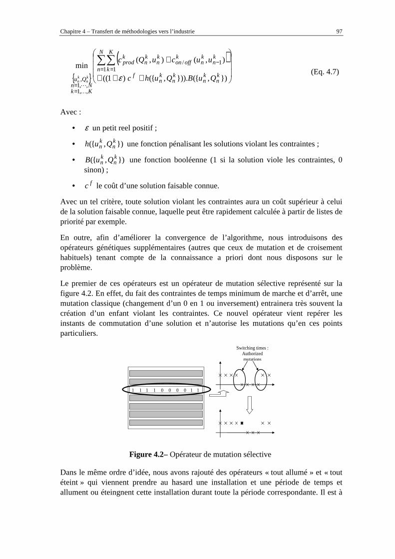
Chapitre 4 – Transfert de méthodologies vers l’industrie 97
( )
+++
+∑∑= =
−
==
),()).,()1((
),(),(min 1 1
1/
,,1,,1
,kn
kn
kn
kn
f
N
n
K
k
kn
kn
koffon
kn
kn
kprod
KkNn
Qu QuBQuhc
uucuQc
kn
kn εK
L
(Eq. 4.7)
Avec :
• ε un petit reel positif ;
• ),( kn
kn Quh une fonction pénalisant les solutions violant les contraintes ;
• ),( kn
kn QuB une fonction booléenne (1 si la solution viole les contraintes, 0
sinon) ;
• fc le coût d’une solution faisable connue.
Avec un tel critère, toute solution violant les contraintes aura un coût supérieur à celui de la solution faisable connue, laquelle peut être rapidement calculée à partir de listes de priorité par exemple.
En outre, afin d’améliorer la convergence de l’algorithme, nous introduisons des opérateurs génétiques supplémentaires (autres que ceux de mutation et de croisement habituels) tenant compte de la connaissance a priori dont nous disposons sur le problème.
Le premier de ces opérateurs est un opérateur de mutation sélective représenté sur la figure 4.2. En effet, du fait des contraintes de temps minimum de marche et d’arrêt, une mutation classique (changement d’un 0 en 1 ou inversement) entrainera très souvent la création d’un enfant violant les contraintes. Ce nouvel opérateur vient repérer les instants de commutation d’une solution et n’autorise les mutations qu’en ces points particuliers.
1 1 1 1 1 1 0 0 0 0
Switching times : Authorized mutations
Figure 4.2– Opérateur de mutation sélective
Dans le même ordre d’idée, nous avons rajouté des opérateurs « tout allumé » et « tout éteint » qui viennent prendre au hasard une installation et une période de temps et allument ou éteingnent cette installation durant toute la période correspondante. Il est à

98 Chapitre 4 – Transfert de méthodologies vers l’industrie
noter que ces trois opérateurs ne garantissent pas la création de nouvelles solutions faisables, ils en augmentent seulement la probabilité.
Enfin, comme il est bien connu que certaines installations sont plus rentables que d’autres, nous avons ajouté un opérateur d’échange de planning, représenté sur la figure 4.3.
0 1 1 1 0
1 0 0 1 1
N
K
Figure 4.3– Opérateur d’échange de planning
Cet opérateur choisit aléatoirement deux installations et une tranche de temps et échange les plannings de ces deux unités.
Afin de tester l’apport de ces nouveaux opérateurs, le tableau 4.1 présente les résultats obtenus avec les nouveaux opérateurs pour un cas de relative petite dimension : 4 unités et 24 périodes temporelles soit 96 variables binaires pour lequel la solution optimale est connue. A chaque fois 100 tests sont effectués. Un test est un succès si la solution optimale est trouvée.
TABLE 4.1 – Résultats d’optimisation avec nouveaux opérateurs
Cas Meilleur Moyenne Ecart-Type
Nombre de succès
Temps de calcul
50 ind. 100 iter.
8778 € (+0%)
9050 € (+3.1%)
236 € 20 13 s
100 ind. 100 iter.
8778 € (+0%)
9006 € (+2.6%)
265 € 31 26 s
50 ind. 200 iter.
8778 € (+0%)
8824 € (+0.5%)
73 € 77 24 s
50 ind. 300 iter.
8778 € (+0%)
8788 € (+0.1%)
37 € 94 40 s
Les mêmes résultats sont donnés sur le tableau 4.2, cette fois avec seulement les opérateurs classiques. L’amélioration apportée par les nouveaux opérateurs est très nette. Cela ne signifie pas que l’algorithme classique ne fonctionne. Il faut simplement beaucoup plus d’itérations pour le faire converger vers des solutions acceptables.

Chapitre 4 – Transfert de méthodologies vers l’industrie 99
TABLE 4.2 – Résultats d’optimisation avec opérateurs classiques seuls
Cas Meilleur Moyenne Ecart-Type
Nombre de succès
Temps de calcul
50 ind. 100 iter.
12221 € 13272 € 466 € 0 12 s
100 ind. 100 iter.
10798 € 12838 € 559 € 0 12 s
Enfin, le tableau 4.3 présente les résultats obtenus avec l’algorithme proposé pour des cas de grande dimension (jusqu’à 100 unités, soit 2400 variables binaires, soit
7222400 10.96,22 ≈ combinaisons possibles). Les tests sont effectués à l’aide de cas particuliers pour lesquels la solution optimale est connue. La taille des populations est fixée à 50. Les résultats obtenus montrent que des solutions de très bonne qualité peuvent être obtenues par cet algorithme et les nouveaux opérateurs.
TABLE 4.3 – Résultats d’optimisation pour des cas de grande dimension
Nombre d’unités
Nombre d’itérations Meilleur Moyenne
Ecart-type
Temps de calcul
10 500 29815 €
(+0.07%) 30016 €
(+0.74%) 185 € 188 s
20 500 1.50 105 € (+ 0.1%)
1.51 105 € (+ 0.9%)
710 € 466 s
40 1000 5.56 105 € (+ 0.07%)
5.59 105 € (+ 0.7%)
1.76 103 € 3100 s
60 1500 1.21 106 € (+ 0.21%)
1.22 106 € (+ 0.37%)
3.45 103 € 12000 s
80 2000 2.14 106 € (+ 0.32%)
2.15 106 € (+ 0.61%)
6.83 103 € 21000 s
100 2000 3.34 106 € (+ 0.85%)
3.36 106 € (+ 1.51%)
1.50 104 € 34000 s
4.2.3.4. Résolution hybride
Nous avons enfin proposé d’hybrider l’algorithme de colonie de fourmis avec l’algorithme génétique [SFT08b]. L’idée est d’utiliser la meilleure solution trouvée dans l’algorithme de colonie de fourmis comme solution faisable dans le coût (4.7). De plus, nous utilisons l’algorithme de fourmis comme générateur de solutions faisables pour

100 Chapitre 4 – Transfert de méthodologies vers l’industrie
former la population initiale de l’algorithme génétique. Les résultats obtenus montrent que cette approche permet de diminuer encore le nombre d’itérations nécessaires pour trouver des solutions de qualité.
4.3. Utilisation d’algorithmes d’optimisation métaheuristiques pour la synthèse de correcteurs
4.3.1. Utilisation de l’optimisation par essaim particulaire pour la synthèse H∞∞∞∞.
Les travaux présentés dans la section 3.4 concernant la synthèse H∞, et notamment l’optimisation des filtres de pondération trouvent un écho très favorable dans l’industrie, et ce pour plusieurs raisons :
• Le réglage des filtres de pondération dans une approche classique est une étape demandant une certaine expérience pour traduire les objectifs du cahier des charges en termes de gabarits fréquentiels de la boucle fermée. Cette étape étant supprimée, il n’est plus nécessaire de faire cette reformulation (les spécifications prises en compte sont les spécifications « naturelles » du cahier des charges), et le réglage peut être effectué par des personnels moins qualifiés.
• Toutes les contraintes du cahier des charges sont prises en compte lors de la synthèse. Il n’est plus nécessaire d’alterner des phases de synthèse de correcteur et des phases de vérification a posteriori de la satisfaction des contraintes. Il s’agit donc d’un gain de temps non négligeable dans la phase de conception de la loi de commande.
• L’utilisation d’une version relativement simple de l’algorithme par optimisation particulaire et de valeurs de paramètres standard conduit à une méthode sans aucun paramètre à régler.
• Même s’il n’y a pas de garantie d’avoir l’optimum global, la solution trouvée satisfait toutes les spécifications et conduit généralement à des performances meilleures que celles obtenues avec un réglage classique.
Dans ce contexte, deux études ont été menées au Département Automatique de Supélec en utilisant l’algorithme développé.
Une première étude, réalisée pour Renault [PTS09] a ainsi permis de calculer des correcteurs pour l’alimentation en air d’un moteur thermique, tandis qu’une deuxième, réalisée pour Arcelor [JDG11] a concerné sur le problème de la coulée continue. Ces deux exemples prouvent l’efficacité de la méthodologie développée.
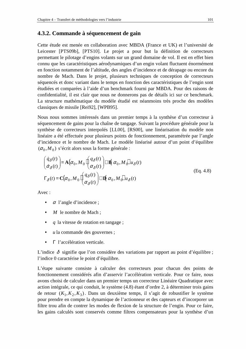
Chapitre 4 – Transfert de méthodologies vers l’industrie 101
4.3.2. Commande à séquencement de gain
Cette étude est menée en collaboration avec MBDA (France et UK) et l’université de Leicester [PTS09b], [PTS10]. Le projet a pour but la définition de correcteurs permettant le pilotage d’engins volants sur un grand domaine de vol. Il est en effet bien connu que les caractéristiques aérodynamiques d’un engin volant fluctuent énormément en fonction notamment de l’altitude, des angles d’incidence et de dérapage ou encore du nombre de Mach. Dans le projet, plusieurs techniques de conception de correcteurs séquencés et donc variant dans le temps en fonction des caractéristiques de l’engin sont étudiées et comparées à l’aide d’un benchmark fourni par MBDA. Pour des raisons de confidentialité, il est clair que nous ne donnerons pas de détails ici sur ce benchmark. La structure mathématique du modèle étudié est néanmoins très proche des modèles classiques de missile [Rei92], [WPB95].
Nous nous sommes intéressés dans un premier temps à la synthèse d’un correcteur à séquencement de gains pour la chaîne de tangage. Suivant la procédure générale pour la synthèse de correcteurs interpolés [LL00], [RS00], une linéarisation du modèle non linéaire a été effectuée pour plusieurs points de fonctionnement, paramétrée par l’angle d’incidence et le nombre de Mach. Le modèle linéarisé autour d’un point d’équilibre
),( 00 Mα s’écrit alors sous la forme générale :
( ) ( )
( ) ( ) )(,)(
)(,)(
)(,)(
)(,
)(
)(
0000
0000
tuMt
tqMt
tuMt
tqM
t
tq
δδ
δδ
δδ
δ
δ
δ
αα
α
αα
αα
DC
BA
+
=Γ
+
=
&
&
(Eq. 4.8)
Avec :
• α l’angle d’incidence ;
• M le nombre de Mach ;
• q la vitesse de rotation en tangage ;
• u la commande des gouvernes ;
• Γ l’accélération verticale.
L’indice δ signifie que l’on considère des variations par rapport au point d’équilibre ; l’indice 0 caractérise le point d’équilibre.
L’étape suivante consiste à calculer des correcteurs pour chacun des points de fonctionnement considérés afin d’asservir l’accélération verticale. Pour ce faire, nous avons choisi de calculer dans un premier temps un correcteur Linéaire Quadratique avec action intégrale, ce qui conduit, le système (4.8) étant d’ordre 2, à déterminer trois gains de retour ),,( 321 KKK . Dans un deuxième temps, il s’agit de robustifier le système pour prendre en compte la dynamique de l’actionneur et des capteurs et d’incorporer un filtre trou afin de contrer les modes de flexion de la structure de l’engin. Pour ce faire, les gains calculés sont conservés comme filtres compensateurs pour la synthèse d’un

102 Chapitre 4 – Transfert de méthodologies vers l’industrie
correcteur H∞ Loop Shaping [GM89], [MG92]. Remarquons que nous avons utilisé un correcteur sous-optimal, permettant d’avoir naturellement un correcteur sous forme observateur / retour d’état favorisant l’interpolation.
Finalement, le calcul du correcteur pour un point de fonctionnement donné revient à choisir des matrices de pondération ),( RQ pour le régulateur Linéaire Quadratique initial. Cela peut se faire assez facilement par essais et erreurs. Le problème qui se pose est le fait que ce réglage doive se faire pour chaque point de fonctionnement. Cette procédure peut donc devenir rapidement fastidieuse du fait du nombre de correcteurs à calculer, et il est donc nécessaire de définir une procédure systématique pour ce réglage. Nous avons décidé ici de reformuler le problème de réglage des correcteurs locaux en un problème d’optimisation (un pour chaque point de fonctionnement) :
≥∆°≥∆
dBGcs
tr
6),(
45),(.
),(min,
RQ
RQ
RQRQ
ϕ (Eq. 4.9)
Avec :
• ),( RQrt le temps de réponse à 5% en boucle fermée obtenu en considérant le système linéarisé et le correcteur calculé à partir des matrices de pondération
),( RQ ;
• ),( RQϕ∆ la marge de phase obtenue en considérant le système linéarisé et le correcteur calculé à partir des matrices de pondération ),( RQ ;
• ),( RQG∆ la marge de gain obtenue en considérant le système linéarisé et le correcteur calculé à partir des matrices de pondération ),( RQ .
Le problème d’optimisation obtenu est bien sûr très délicat à résoudre (nombreux minima locaux, fonctions de coûts et de contraintes n’ayant pas d’expression analytique…). Nous avons donc eu recours à un algorithme d’optimisation par essaim particulaire tel que celui décrit dans le chapitre 3. En outre, l’utilisation des valeurs de paramètres « standard » a permis d’obtenir une méthode sans réglage de paramètre.
La suite de l’étude, non détaillée ici, a consisté à étendre les résultats aux autres voies (lacet et roulis), puis à comparer le correcteur interpolé mono-axe à une synthèse LPV [AGB95], [AG95], [Pac94], [FAG96]. Concernant la synthèse LPV, le réglage des pondérations a pu être optimisé par essaim particulaire également.

Chapitre 4 – Transfert de méthodologies vers l’industrie 103
4.4. Extension de résultats d’optimisation dans un contexte de boucle fermée
4.4.1. Principe général
L’optimisation d’un système peut souvent être vue comme une commande en boucle ouverte de ce système : elle permet de déterminer une séquence de commande optimale permettant de satisfaire un objectif donné. C’est typiquement ce que l’on fait lorsqu’on résout le problème d’Unit Commitment de la section 4.2. Il est évident que cette commande ne peut être appliquée directement au système. En effet :
• Ce résultat d’optimisation a été obtenu à partir d’un modèle souvent très simplifié du système. Ces simplifications ont été nécessaires afin d’avoir un modèle suffisamment rapide pour l’optimisation.
• Il existe de nombreuses incertitudes paramétriques.
• Il existe de nombreuses perturbations agissant sur le système.
Ces incertitudes peuvent avoir un impact d’autant plus grave que la solution optimale calculée se trouve généralement en limite de contraintes : c’est en saturant une ou des contraintes qu’on obtient les meilleures performances.
Afin d’utiliser les résultats d’optimisation dans un contexte de boucle fermée, une façon relativement courante de faire est d’utiliser le principe de l’horizon fuyant : l’optimisation est réalisée à chaque période d’échantillonnage, la première commande de la séquence calculée est envoyée au système, puis on remet à jour le modèle utilisé pour l’optimisation à la période d’échantillonnage suivante où le problème d’optimisation est à nouveau résolu. Nous avons déjà vu cette approche aux paragraphes 2.2.1 et 2.2.2.
Nous avons de plus appliqué cette stratégie pour des problèmes de gestion de l’énergie et sur un benchmark ABB de ventilation minière.
4.4.2. Gestion de l’énergie
Nous reprenons ici le problème d’affectation d’unités de la section 4.2. L’optimisation présentée suppose que toutes les grandeurs sont connues. Ceci est bien sûr faux, notamment en ce qui concerne la demande des consommateurs dem
nQ de l’équation (4.3) qui est en réalité prédite à partir de données météorologiques et de différents facteurs sociaux.
Nous avons présenté dans [SO07] l’utilisation du principe de l’horizon fuyant pour résoudre le problème, l’optimisation en ligne étant réalisée par l’algorithme hybride colonie de fourmis / algorithme génétique de la section 4.2.3.4. Le problème résolu fait partie d’une classe de problèmes plus générale, à savoir la commande prédictive sous

104 Chapitre 4 – Transfert de méthodologies vers l’industrie
contrainte des systèmes hybrides [BBM98]. La méthodologie proposée peut s’étendre, sous réserve, comme toujours pour ce type de problème, que l’optimisation en ligne puisse être réalisée en un temps inférieur à la période d’échantillonnage.
Avec le même type d’approche, nous avons proposé le pilotage d’un réseau de chauffage urbain, tel que celui décrit dans la section 2.2.1 [SO09], [SFT05c]. Sur le fond le problème est identique : il s’agit de robustifier le pilotage d’un réseau de production d’énergie afin de le rendre insensible aux erreurs de prédiction sur la courbe de charge. La différence réside néanmoins au niveau de la structure mathématique du problème, puisque les grandeurs de commande sont des températures de fourniture d’eau chaude. Il s’agit donc d’un problème en variables réelles. En revanche, le modèle utilisé fait intervenir des équations aux dérivées partielles pour décrire la propagation de l’énergie au sein du réseau de distribution. Les algorithmes d’optimisation utilisés sont des méthodes de quasi Newton dans [SFT05c] et d’essaim particulaire dans [SO07].
Enfin, le couplage entre la production et la distribution dans le cas de réseau de chauffage urbain a été étudiée dans [San09].
Remarquons pour finir ce paragraphe, que les systèmes étudiés dans ce paragraphe 4.4.2, et notamment les réseaux de chauffage urbain, sont complexes en termes de modélisation, mais relativement faciles à piloter. Il faut entendre par là qu’ils sont « inconditionnellement stables ». En effet, dans le cas des réseaux de chauffage urbain, si on ne produit pas assez, le client n’aura pas toute l’énergie demandée, mais cela ne met pas en péril le fonctionnement du réseau de distribution du fait du fonctionnement des échangeurs de chaleur. Inversement, si on produit trop d’énergie, le surplus sera naturellement stocké (aux pertes thermiques près) dans le réseau de distribution d’eau chaude.
4.4.3. Ventilation minière
Le problème considéré ici est un benchmark ABB représenté sur la figure 4.4.
Figure 4.4– Problème de ventilation minière
La ventilation est réalisée par une turbine connectée à la surface via un puits vertical. Des ventilateurs envoient l’air frais à chaque niveau de forage. A l’intérieur de la mine,

Chapitre 4 – Transfert de méthodologies vers l’industrie 105
des engins travaillent et rejettent des polluants nocifs pour l’être humain. Ces polluants sont naturellement expulsés à l’extérieur du fait du gradient de pression occasionné par l’introduction d’air frais. L’objectif de la régulation est de maintenir une qualité de l’air suffisante (c'est-à-dire avec des concentrations faibles en polluants) en agissant sur les ventilateurs.
La concentration d’un polluant j à l’altitude z est modélisé par :
))()((1
)(),(
tzt
jj
jje
ttzc γβ
α−−+
= (Eq. 4.10)
avec )(tjα l’amplitude, )(tjβ la dilatation et )(tjγ l’inflexion de la distribution. Ces grandeurs constituent les variables d’état du problème et obéissent à une équation non linéaire de la forme :
[ ]
=
)(),(),(),(),(
,),(),(),(
)()()()()()(
111
111
tmtuttt
tttf
tttttt
innnn
Tnnn
&
K
&&&K&&&
γβαγβα
γβαγβα (Eq. 4.11)
Où )(tmin& représente les émissions de polluants par les engins. Il s’agit d’une perturbation pour notre système.
Le problème se traduit naturellement comme un compromis entre la qualité de l’air et l’énergie utilisée par les ventilateurs. Nous allons le traduire en un critère d’optimisation très semblable à celui de la commande prédictive :
( )
[/,/)1([pour
)(:avec
)()()(ˆmin 22,
,,1
uu
i
NkT
kTj
desjj
Niu
NiNkTNNikT
uu
duyy
u
i
+−+∈=
+−∫ ∑
+
=
ττ
ττλττK
(Eq. 4.12)
avec uN le nombre de degrés de liberté dans la loi de commande, N l’horizon de prédiction, T la période, )(ˆ τjy la concentration en polluant j prédite par le modèle (4.11) à partir de prédiction des émissions de polluants, )(τu la commande des ventilateurs supposée constante sur une période d’échantillonnage, )(, τdesjy la concentration désirée, et λ un facteur de pondération.
Les contraintes à satisfaire sont un niveau de polluant maximum maxjy à respecter à une
altitude rz fixée :
max),()( jrjj ytzcty ≤= (Eq. 4.13)
Le problème (4.12) est résolu en utilisant le simplexe de Nelder Meald, et le système bouclé par le principe de l’horizon fuyant. Les résultats obtenus dans [WIS09], où cette approche a été comparée avec une approche basée sur la commande de système hybride

106 Chapitre 4 – Transfert de méthodologies vers l’industrie
montrent des résultats tout à fait satisfaisants en termes de compromis qualité de l’air / énergie de commande.
4.5. Conclusions
Nous avons présenté dans ce chapitre un certain nombre d’applications industrielles qui utilisent les méthodologies développées au Département Automatique de Supélec. Ainsi, nous avons successivement présenté la résolution du problème d’affectation d’unités, l’utilisation de l’optimisation par essaim particulaire pour la synthèse H∞ et le calcul de correcteurs interpolés, et l’utilisation du principe de l’horizon fuyant pour boucler le système à partir de résultats d’optimisation.
Comme l’a montré notamment la section 4.3, les méthodes basées sur l’utilisation de métaheuristiques intéressent grandement nos partenaires industriels et ce pour plusieurs raisons. La raison principale est le fait que l’on peut résoudre le problème initial sans aucune reformulation du cahier des charges et tenant compte dès la phase de synthèse de toutes les contraintes. De plus, en utilisant des méthodes sans réglage de paramètres, la résolution peut être faite par des personnels ne connaissant pas forcément les méthodes sous jacentes, que cela soit en termes d’Automatique ou d’optimisation.
Outre l’intérêt théorique d’étudier les algorithmes stochastiques pour la résolution de problèmes d’automatique, cet intérêt industriel prouve le potentiel de ces méthodes. Ce chapitre, d’une part, ferme la boucle par rapport au chapitre 2 dans la mesure où il retourne à des applications industrielles. Dans le chapitre 2, la problématique initiale était reformulée pour conduire à la résolution exacte d’un problème approché. Dans ce chapitre, nous avons exploité une deuxième approche qui est la résolution approchée du problème initial. D’autre part, ce chapitre a déjà un pied dans les perspectives des travaux de recherche, puisque la finalité de ces travaux est toujours le transfert des méthodes vers l’industrie.
Pour terminer l’exposé de ces travaux de recherche, il convient d’insister sur le rôle de l’optimisation pour la résolution de problèmes d’automatique. Résoudre un problème d’optimisation peut sembler pour le novice un peu magique dans le sens où, sans connaître réellement l’Automatique, il sera capable de régler un correcteur en utilisant des méthodes avancées. En réalité il n’en est rien. En effet, un algorithme d’optimisation ne résout que ce qu’on lui donne à résoudre. Poser le problème de façon intelligente nécessite une connaissance fine à la fois du système que l’on étudie et des méthodes d’optimisation. Enfin, il ne faut pas oublier qu’un algorithme d’optimisation appartient au redoutable monde du calcul numérique. Il convient donc de toujours valider les solutions obtenues et leur cohérence à l’aune de la connaissance a priori disponible pour le problème traité.

TroisTroisTroisTroisièmeièmeièmeième partiepartiepartiepartie ::::
ProjetProjetProjetProjet de recherchede recherchede recherchede recherche


Chapitre 5
Projet de recherche
5.1. Introduction ...................................................................................................... 111
5.2. Perspectives à court terme ............................................................................... 111
5.2.1. Collaborations industrielles en cours ........................................................... 111
5.2.2. Synthèse de correcteurs d’ordre réduit......................................................... 112
5.2.3. Analyse de robustesse .................................................................................. 113
5.2.4. Optimisation robuste .................................................................................... 114
5.2.5. Métaheuristiques pour l’industrie ................................................................ 115
5.3. Perspectives à moyen terme............................................................................. 115
5.3.1. Problèmes d’automatique potentiellement traités avec des métaheuristiques ................................................................................................................................ 115
5.3.2. Collaborations avec la communauté « métaheuristiques » .......................... 116
5.3.3. Optimisation et commande prédictive ......................................................... 116
5.4. Perspectives à long terme................................................................................. 117
5.4.1. Modélisation de systèmes complexes .......................................................... 117
5.4.2. Inversion des rôles automatique / optimisation............................................ 118

110 Chapitre 5 – Projet de recherche

Chapitre 5 – Projet de recherche 111
5.1. Introduction
Nous avons présenté dans les chapitres précédents une synthèse des travaux de recherche. Ceux-ci s’articulent autour de trois axes : la modélisation, l’optimisation et la commande de systèmes industriels, le développement de méthodologies pour l’automatique fondée sur les métaheuristiques, et le transfert de ces méthodes vers l’industrie. En schématisant, les collaborations industrielles du chapitre 2 s’appuient généralement sur une formalisation de problématiques industrielles qui se traduisent par une modélisation adaptée de ce problème pour que celui-ci puisse être résolu par des méthodes classiques ad’ hoc. Nous avons ensuite montré les limites possibles de cette approche lorsque les systèmes deviennent « trop » complexes ou que l’on désire optimiser les paramètres de réglages des méthodes de synthèse classiques. Cela nous a conduits au développement de méthodes utilisant des algorithmes stochastiques présentées au chapitre 3. Enfin, nous avons commencé à présenter des transferts de ces méthodes vers l’industrie au chapitre 4 en insistant sur le fort potentiel et le ressenti favorable qu’elles peuvent avoir au sein des industriels.
Le projet de recherche va naturellement tenter de poursuivre les voies ouvertes pour étendre, exploiter et capitaliser les travaux entrepris. Nous séparons dans la suite les perspectives à court terme qui concernent des travaux en cours ou qui vont démarrer prochainement, des perspectives à plus long terme.
5.2. Perspectives à court terme
5.2.1. Collaborations industrielles en cours
Quelques collaborations industrielles sont actuellement en cours. Parmi celles-ci se trouve l’étude réalisée avec MBDA et l’université de Leicester présentée au paragraphe 4.3.2. Les étapes à venir vont permettre de valider plus avant la démarche de synthèse de correcteurs interpolés à partir d’optimisation par essaim particulaire. En effet, l’objectif est de complexifier le problème étudié en effectuant une synthèse trois axes pour tenir compte des couplages entres les voies de tangage, de lacet et de roulis. La synthèse du correcteur devra donc être pleinement multivariable, ce qui entraînera une augmentation du nombre de variables de décision dans l’algorithme d’optimisation par essaim particulaire.
Une autre collaboration a actuellement lieu avec Renault et la société LMS qui commercialise le logiciel de simulation AMESim. Cette collaboration a lieu dans le cadre beaucoup plus général du projet CSDL (Complex System Design Lab). Ce projet a pour but le développement d’un environnement collaboratif important permettant la simulation et l’optimisation de systèmes complexes. Il regroupe plusieurs industriels (Renault, Dassault, MBDA…) qui proposent chacun un cas d’étude représentatif des

112 Chapitre 5 – Projet de recherche
problématiques abordées, des éditeurs de logiciel de simulation (LMS, Enginsoft, Ansys…) qui apportent chacun leur spécificité en termes de niveau de modélisation et simulation (simulation par éléments finis, orientée commande…), et des institutions académiques (Supélec, Centrale Paris, Mines de Paris…) qui mettent à disposition leur savoir faire en termes de méthodologies d’étude. Parmi les points étudiés se trouvent la réduction de modèles (au sens passage d’un modèle à éléments finis à un modèle utilisable pour la commande), la propagation d’incertitudes dans les codes de calcul, et les méthodologies permettant de renseigner les modèles.
L’implication du Département Automatique, associé au Département Electrotechnique et Systèmes d’Energie, a lieu dans le cadre du cas d’étude Renault sur le véhicule électrique, dans la continuité des travaux de thèse de NOËLLE JANIAUD [Jan11]. Il s’agit de développer des modèles de machines électriques prenant en compte la saturation magnétique et les pertes fers et d’optimiser les lois de commande associées. Les méthodologies devront être implantées au sein du logiciel AMESim.
D’autres collaborations industrielles effectuées dans le cadre de thèses de doctorat sont présentées dans les sections 5.2.2 et 5.2.3.
5.2.2. Synthèse de correcteurs d’ordre réduit
Un axe important des travaux actuels concernent la synthèse de correcteurs d’ordre réduit ou structurés, calculés notamment dans un formalisme de type H∞. En effet, la synthèse de correcteurs robustes multivariables par un tel formalisme est une technique de commande avancée des systèmes qui a désormais fait ses preuves dans le domaine industriel (aéronautique, aérospatial…). L’une des difficultés sous-jacentes à ce type de méthodes demeure l’ordre du correcteur obtenu. En effet, une contrainte sur l’ordre du correcteur entraîne la perte de la convexité du problème de synthèse. Historiquement, la difficulté était contournée soit en réduisant a posteriori le correcteur obtenu, soit en adaptant les outils de l’optimisation convexe sans garantie d’optimalité. Plus récemment, l’optimisation non convexe a permis quelques avancées dans le domaine [Bom07], [Sim09] (optimisation non lisse), [YS11] (optimisation par essaim particulaire).
Dans ce contexte, la thèse CIFRE de SERGE HIRWA, effectuée en collaboration avec la Sagem et encadrée par GILLES DUC et moi-même, a démarré en juillet 2010. Cette thèse s’intitule « Méthodes de commande avancées appliquées aux viseurs » qui s’inscrit dans le cadre de l’activité Viseurs Héliportés de Sagem Défense Sécurité. Le système concerné est un viseur type Boule Gyro-Stabilisée 4 axes. La synthèse des correcteurs doit faire face aux contraintes industrielles suivantes :
• performances demandées toujours accrues, tant en précision de pointage qu’en performances dynamiques ;
• contraintes d’implémentation hardware obligeant à optimiser grandement les correcteurs et notamment leur ordre.

Chapitre 5 – Projet de recherche 113
Les premiers travaux entrepris ont concerné l’identification du système. Le modèle correspondant est caractérisé par de nombreux modes souples. Parallèlement, le système est soumis à de fortes perturbations harmoniques dues par exemple aux vibrations induites par le mouvement des pales de l’hélicoptère. Ces perturbations imposent l’introduction de réjecteurs dans le correcteur et augmentent d’autant son ordre.
Plusieurs techniques de synthèse de correcteurs d’ordre réduit dans un contexte de synthèse H∞ standard ou Loop Shaping ont déjà été testées sur des modèles simplifiés :
• réduction a posteriori ;
• utilisation de solveurs basés sur l’optimisation non convexe tels HIFOO [BHL06] ou la routine ‘hinfstruct’ de Matlab [Sim09] ;
• utilisation d’une heuristique développée dans [VM97] qui synthétise un correcteur réduit à partir d’un pré-correcteur. Ce pré-correcteur peut par exemple être calculé à partir de la méthode développée dans [TL09].
Après de premiers tests concluants, les travaux futurs s’orientent vers une complexification du problème traité en abordant des structures de commande multivariables (plusieurs mesures disponibles), une introduction d’une correction par anticipation permettant de lutter efficacement contre les vibrations, et une étude approfondie de la robustesse de la loi de commande obtenue. En effet, une grande dispersion des valeurs numériques du système est observée lors de la production en série.
Cette thématique de synthèse de correcteurs d’ordre réduit est également un thème majeur de l’équipe-projet INRIA DISCO à laquelle je participe en tant que chercheur associé.
5.2.3. Analyse de robustesse
L’analyse de la robustesse d’une loi de commande est un point clé de l’automatique dans un contexte industriel. C’est pourquoi la thèse de JULIEN CHAUDENSON, effectuée en collaboration avec Astrium, l’ESA et l’université de Stuttgart, a débuté en octobre 2010. Cette thèse est co-encadrée par DOMINIQUE BEAUVOIS, CARSTEN SCHERER et moi-même et porte sur l’analyse de robustesse des systèmes non linéaires avec application aux lanceurs spatiaux en phase balistique. J’ai obtenu une dérogation du Conseil Scientifique de l’université Paris XI pour être le directeur de thèse.
L’objectif général de la thèse est d’étendre les méthodes, actuellement utilisées pour valider les lois de commande des lanceurs, pour prendre en compte les non linéarités du système. Actuellement, la validation des lois de commande est en effet effectuée à l’aide d’outils désormais classiques de l’automatique linéaire (marges de stabilité, µ-analyse…) à partir de modèles linéarisés, ou de campagnes intensives et donc coûteuses en temps de calcul de simulations du modèle non linéaire (validation de type Monte Carlo).

114 Chapitre 5 – Projet de recherche
Les travaux se sont pour l’instant concentrés sur la définition de modèles non linéaires, à une et trois dimensions, représentatifs du système, obtenus à partir du simulateur complet du lanceur. L’objectif de la définition de ces modèles était d’avoir des benchmarks suffisamment simples mais intégrant les principales non linéarités du système afin de tester les différentes méthodes d’analyse de robustesse. Dans un deuxième temps, les outils classiques d’étude de stabilité ont été utilisés pour obtenir des conditions, souvent conservatives, de stabilité à partir de modèles linéarisés.
Il s’agit désormais de traiter le cas des non linéarités. Pour ce faire, la piste envisagée concerne l’utilisation des IQCs (Contraintes Intégrales Quadratiques) [Jon97], [MR97], [KMJ04], [KS09] par exemple. Parmi les différentes non-linéarités et retards présents dans les modèles, certains peuvent être pris en compte par les toolboxes disponibles. En revanche, d’autres non linéarités plus « exotiques » (PWM par exemple) nécessiteront une réflexion poussée afin de définir des multiplieurs adaptés au problème.
5.2.4. Optimisation robuste
Lorsque l’on cherche à optimiser le fonctionnement d’un système, l’optimum est généralement de se placer en limite de contraintes. Ceci est généralement incompatible avec le pilotage d’un système réel. En effet, l’optimisation a toujours été effectuée à partir d’un modèle du système. Il existe forcément des incertitudes de modélisation (certains phénomènes sont négligés par exemple) et des incertitudes paramétriques (les paramètres du modèle sont identifiés à partir de résultats expérimentaux). Dès lors, l’application du pilotage optimal calculé au système réel entrainera une variation par rapport à ce qui été prédit par le modèle et l’optimisation, et donc bien souvent une violation des contraintes. Ainsi, optimisation et robustesse sont-elles des notions contradictoires.
C’est dans ce contexte que se place l’optimisation robuste. Une vaste littérature existe sur le sujet, [Sah04], [BD96], [CSW03], [MVZ95] par exemple, abordant différentes techniques et notamment la notion d’optimisation avec recours. La thèse d’HENRI
BORSENBERGER, co-encadrée par PHILIPPE DESSANTE du Département Electrotechnique et Systèmes d’Energie de Supélec et moi-même est actuellement en cours de finalisation. Cette thèse porte sur l’optimisation robuste de systèmes complexes avec application aux réseaux d’énergie. Le cas d’étude considéré est celui de l’affectation d’unités présenté au paragraphe 4.2. Cet exemple présente en effet de nombreuses incertitudes que nous avons étudiées :
• Incertitudes sur la demande d’énergie de la part des consommateurs ;
• Incertitudes sur les coûts de production [BDS11]. C’est typiquement le cas lorsque le système de production d’énergie présente des incinérateurs ou des systèmes de cogénération.
• Incertitudes sur la capacité maximale de production. C’est le cas pour des installations photovoltaïques ou éoliennes.

Chapitre 5 – Projet de recherche 115
Les travaux effectués ont porté sur des méthodes d’optimisation robuste déterministes (à base de relaxation lagrangienne) applicables aux problèmes d’optimisation mixte (nombreuses variables binaires).
Les perspectives de ces travaux concernent d’une part l’utilisation de méthodes approchées pour des cas de très grande dimension, et d’autre part la prise en compte du réseau de distribution. Dans ce dernier cas, les modèles d’optimisation sous-jacents n’ont pas toujours d’expressions analytiques (c’est le cas des réseaux de chauffage urbain). D’autre part, ils sont relativement longs à simuler ce qui limite le nombre d’évaluations des fonctions de coût et de contraintes.
5.2.5. Métaheuristiques pour l’industrie
Nous avons exposé au paragraphe 4.3 un certain nombre d’exemples concrets où l’utilisation de méthodes d’optimisation métaheuristiques a trouvé un écho très favorable chez les industriels. Dans ce cadre, une thèse a débuté en janvier 2012 entre le département Automatique de Supélec et la Sagem portant sur l’optimisation des asservissements des viseurs par les métaheuristiques.
La Sagem est en effet parti d’un constat que nous avions déjà fait, à savoir que les méthodes d’automatique dites avancées employées pour la synthèse des correcteurs robustes linéaires ont permis à l’ingénieur de synthétiser ou d’adapter des correcteurs rapidement, facilement et surtout robustes aux incertitudes du système. En revanche, les méthodes de travail employées nécessitent, d’une part, encore plusieurs itérations de synthèses, et d’autre part un certain degré d’expérience de la part du concepteur.
Les objectifs de la thèse seront donc d’utiliser les algorithmes métaheuristiques pour améliorer et accélérer le réglage des correcteurs. En outre, l’utilisation de tels algorithmes rendra possible la prise en compte d’éléments non linéaires tels que les frottements lors de la phase de synthèse.
Le démarrage de cette thèse montre une nouvelle fois l’intérêt que porte le monde industriel pour le type de méthodes développées.
5.3. Perspectives à moyen terme
5.3.1. Problèmes d’automatique potentiellement traités avec des métaheuristiques
Nous avons présenté dans ce manuscrit plusieurs problèmes d’automatique résolus en ayant recours à des méthodes de type métaheuristiques. Voici une liste non exhaustive de problèmes qu’il nous semble possible de résoudre à l’aide de tels algorithmes :
• Identification de systèmes dynamiques non linéaires ;

116 Chapitre 5 – Projet de recherche
• Identification de modèles de frottements ;
• Synthèse de correcteurs structurés multi-variables ;
• Synthèse mixte H2 / H∞ avec prise en compte de contraintes diverses ;
• Synthèse de filtres à partir de gabarits fréquentiels quelconques ;
• Commande prédictive non linéaire ;
• Optimisation du volume du domaine de stabilité garanti ;
• µ-synthèse ;
• …
5.3.2. Collaborations avec la communauté « métaheuristiques »
Dans les exemples donnés dans les chapitres 3 et 4, nous avons toujours privilégié les variantes d’algorithmes les plus simples et avec des valeurs de paramètres relativement standard. En effet, nous sommes partis des constats suivants :
• Il y aurait peu à gagner à transformer un problème de réglage de paramètres d’une loi de commande en un problème de réglage de paramètres d’un algorithme d’optimisation ;
• Les méthodologies développées ont pour but d’être utilisées dans un contexte industriel et donc par des personnels n’ayant généralement pas de connaissance des méthodes d’optimisation stochastiques ;
• Nous recherchons des méthodes relativement génériques, donc ayant une certaine robustesse vis-à-vis du problème traité. Le but n’était donc pas de trouver la variante la meilleure possible pour résoudre un problème donné.
Les travaux effectués ont permis de prouver la viabilité des approches proposées [San09b], [San11] et le fort potentiel de ces méthodes dans le domaine de l’automatique. Il convient désormais de pousser plus avant les travaux en recherchant des collaborations avec des laboratoires dont les métaheuristiques sont le thème de recherche principal.
5.3.3. Optimisation et commande prédictive
Comme nous l’avons dit à plusieurs reprises, la commande prédictive est caractérisée par la résolution de problèmes d’optimisation en ligne. Très récemment, des travaux ont eu lieu pour aborder l’optimisation de fonctions coûteuses, c'est-à-dire des fonctions dont l’évaluation est très longue [Vil08]. Une telle approche pourrait sans doute être utilisée en Automatique, notamment pour la commande prédictive non linéaire. Dans ce domaine, le point bloquant est toujours la résolution en ligne de problèmes d’optimisation, la résolution devant se faire dans le temps d’une période

Chapitre 5 – Projet de recherche 117
d’échantillonnage. Afin de minimiser les temps de résolution pour les faire tenir en une période d’échantillonnage, une façon de faire pourrait être de diminuer le nombre d’évaluations de la fonction coût (qui ici ne serait pas réellement coûteuse).
Une autre perspective intéressante concerne la robustification des lois de commande prédictive. Des travaux ont eu lieu, notamment au Département Automatique pour robustifier ces lois de commande en utilisant par exemple la paramétrisation de Youla [Sto08]. Ces techniques sont généralement des techniques d’optimisation off-ligne. Il nous semblerait intéressant pour robustifier, cette fois-ci en ligne, la loi de commande d’utiliser des techniques d’optimisation robuste pour résoudre le problème à chaque pas de temps, prenant en compte des incertitudes sur la fonction de coût et les contraintes, et donc sur la modélisation du système.
5.4. Perspectives à long terme
5.4.1. Modélisation de systèmes complexes
Dans le cadre de systèmes complexes, le modèle initial permettant une simulation représentative du comportement du système est généralement inutilisable dans une optique d’optimisation ou de commande. Dès lors, il est nécessaire de disposer d’une batterie de modèles, chacun étant développé pour un objectif particulier (dimensionnement, simulation, optimisation, commande….). La structure des modèles reste néanmoins identique, et il serait intéressant de réfléchir à une « méta modélisation », permettant une manipulation efficace des modèles (modélisation objet, approches formelles, langage de description basé sur les approches objet…), indépendamment du but recherché.
L’élaboration des modèles passe généralement par une agrégation de sous systèmes, permettant d’obtenir des modèles globaux, sous l’hypothèse que ces modèles agrégés soient représentatifs, à l’échelle considérée, des phénomènes locaux. La formalisation de cette approche reste à effectuer et il serait intéressant d’explorer plus avant le passage des informations d’un niveau local au niveau global.
Enfin, il est apparu, au cours de nos travaux, que le choix de la causalité des modèles pouvait s’avérer crucial. D’autre part, le choix des variables de commande (ou d’optimisation) peut conduire à des expressions plus ou moins compliquées des critères et des contraintes. Ce choix est souvent à faire au cas par cas. Il peut utiliser un choix non physique du point de vue de la causalité mais correspondant à un simple changement de variables du point de vue de l’optimisation, les variables de commande pouvant être retrouvées a posteriori, en fonction des variables optimisées. La recherche de méthodologies générales de choix de variables et de structures de modèles nous semble une piste de travail à exploiter.
118 Chapitre 5 – Projet de recherche
Tous ces aspects liés à la modélisation et à l’organisation des sous modèles sont des points clés dans le cadre de collaborations industrielles comme nous l’avons vu dans le chapitre 2.
Dans le cadre de la réorganisation de la recherche à Supélec en une seule équipe de recherche baptisée « Supélec sciences des Systèmes », trois thèmes transverses ont été définis, à savoir modélisation, analyse et conception dont je suis l’un des coordinateurs scientifiques. Cette volonté de rapprochement devrait permettre des discussions fructueuses au sujet de la modélisation des systèmes complexes, notamment avec le Département Informatique dont l’une des thématiques de recherche constitue la modélisation des systèmes hétérogènes.
5.4.2. Inversion des rôles automatique / optimisation
Terminons ce chapitre de perspectives par une réflexion plus générale. Dans tous les travaux présentés, l’optimisation apparaît comme un outil au service de l’Automatique. Il serait très intéressant d’inverser les rôles et que les concepts de l’Automatique permettent de résoudre des problèmes d’optimisation, et notamment des problèmes d’optimisation dynamique (la fonction de coût dépend du temps et son optimum fluctue). Dès lors, on peut considérer ce problème d’optimisation comme un système dynamique donc la sortie serait le gradient (en supposant le problème en variables continues, différentiable, et sans contraintes pour simplifier l’exposé), sortie qu’il s’agit de réguler à 0. De telles approches ont déjà été testées, notamment avec la méthode de l’ « Extremum seeking » [KW00], [ZSK07], [TNM06], [AG06], [DG05], [GZ03]. De la même façon, des études de convergence d’algorithme d’optimisation par essaim particulaire ont pu être menées [Tre03] en considérant cet algorithme comme un système dynamique discret.
Il y a là un potentiel très intéressant pour l’Automatique.

Bibliographie
[ABN07] P. APKARIAN, V. BOMPART, D. NOLL, 2007. Nonsmooth structured control design with application to PID loop-shapingof a process. International Journal of Robust and Nonlinear Control, vol. 17, no. 14, pp. 1320-1342.
[ACL05] K. H. ANG; G. CHONG, Y. LI, 2005. PID control system analysis, design, and technology. IEEE Transactions on Control Systems Technology, vol. 13, no. 4, pp.559-576.
[AEF05] J. E. ALVAREZ-BENITEZ, R. M. EVERSON, J. E. FIELDSEND, 2005. A MOPSO algorithm based exclusively on Pareto dominance concepts. Lecture Notes in Computer Science, vol 3410, pp 459-473.
[AG95] P. APKARIAN, P. GAHINET, 1995. A convex characterization of gain scheduled H∞ controllers. IEEE Transactions on Automatic control, vol. 40, pp. 853-864.
[AG06] V. ADETOLA, M. GUAY , 2006. Adaptive output feedback extremum seeking receding horizon control of linear systems. Journal of Process Control, vol.16, pp. 521–533.
[AGB95] P. APKARIAN, P. GAHINET, G. BECKER, 1995. Self-scheduled H∞ control of linear parameter-varying systems: a design example. Automatica, vol. 31, no. 9, pp. 1251-1261.
[AGP10] D. ARZELIER, E. N. GRYAZINA , D. PEAUCELLE, T. POLYAK , 2010. Mixed LMI/Randomized methods for static output feedback control design, Proceedings of the IEEE American Control Conference, Baltimore, USA.
[AH01] K.J. ÅSTRÖM, T. HÄGGLUND, 2001. The future of PID control. Control Engineering Practice, vol. 9, no. 11, pp. 1163-1175.
[AN06] P. APKARIAN AND D. NOLL, 2006. Nonsmooth H∞ synthesis. IEEE Transactions on Automatic Control, vol. 51, no. 1, pp. 71-86.
[ANR08] P. APKARIAN, D. NOLL AND A. RONDEPIERRE, 2008. Mixed H2/H∞ control via nonsmooth optimization. SIAM Journal on Control and Optimization, vol. 47, no. 3, pp. 1516-1546.

120 Bibliographie
[ANS09] P. APKARIAN, D. NOLL AND A. SIMOES, 2009. Time-domain control design: a nonsmooth approach. IEEE Transactions on Control Systems Technology, vol. 17, no. 6, pp. 1439-1445.
[ARN11] P. APKARIAN, L. RAVANBOD-HOSSEINI, D. NOLL, 2011. Time domain constrained H∞ synthesis. International Journal of Robust and Nonlinear Control, vol. 21, no. 2, pp. 197-217.
[Arv01] L. ARVASTSON, 2001. Stochastic modelling and operational optimization in district heating systems. PhD. Thesis, Lund Institute of Technology, Centre for Mathematical Sciences, Mathematical Statistics, ISBN 91-628-4855-0.
[BA95] C. BOHN, D. P. ATHERTON, 1995. An analysis package comparing PID antiwindup strategies. IEEE Control System Magazine, vol. 15, no. 2, pp. 34-40.
[BAN08] V. BOMPART, P. APKARIAN, D. NOLL, 2008. Control design in the time- and frequency domains using nonsmooth techniques. Systems & control letters, vol. 57, no. 3, pp. 271-282.
[BBR95] A. BENONYSSON, B. BOHM, H. F. RAVN , 1995. Operational optimization in a district heating system. Energy Conversion Management, vol. 36, no. 5, pp. 297-314.
[BBM98] M. S. BRANICKY , V. S. BORKAR, S. K. MITTER, 1998. A unified framework for hybrid control: model and optimal control theory. IEEE Transaction on Automatic Control, vol. 43, pp. 31-45.
[BC02] M. BORYCZKA, Z. J. CZECH, 2002. Solving approximation problems by ant colony programming. Proceedings of the Genetic and Evolutionary Computation Conference, New York, USA.
[BCW02] M. BORYCZKA, Z. J. CZECH, W. WIECZOREK, 2002. Ant colony programming for approximation problems. Proceedings of the Intelligent Information Systems 2002 Symposium, Sopot.
[BD96] J. R. BIRGE, M. A. H. DEMPSTER, 1996. Stochastic programming approaches to stochastic scheduling. Journal of Global Optimization, vol. 9, no. 3–4, pp. 417-451.
[BDS11] H. BORSENBERGER, P. DESSANTE, G. SANDOU, 2011. Unit Commitment with production cost uncertainty: a recourse programming method. Journal of Energy and Power Engineering, vol. 5, pp. 164-172.
[BE93] S. BOYD, L. EL GHAOUI, 1993. Methods of centers for minimizing generalized eigenvalues. Linear Algebra and Aplications, special issue on Numerical Linear Algebra Methods in Control, Signals and Systems, vol. 188, pp. 63-111.
[Ber01] A. BERRO, 2001. Optimisation multiobjectif et stratégies d'évolution en environnement dynamique. Thèse de doctorat de l'Université des Sciences Sociales de Toulouse I.
[BFM00a] T. BAECK, D. B. FOGEL, Z. M ICHALEWICZ, 2000. Evolutionary computation 1: basic algorithms and operators. Institute of Physics Publishing.
[BFM00b] T. BAECK, D. B. FOGEL, Z. M ICHALEWICZ, 2000. Evolutionary computation 2: advanced algorithms and operators. Institute of Physics Publishing.
Bibliographie 121
[BHL06] J. V. BURKE, D. HENRION, A. S. LEWIS, M. L. OVERTON, 2006. HIFOO - A Matlab package for fixed-order controller design and H∞ optimization. Proceedings of the IFAC Symposium on Robust Control Design, Toulouse, France.
[BNA07] V. BOMPART, D. NOLL AND P. APKARIAN, 2007. Second-order nonsmooth optimization for H∞ synthesis. Numerische Mathematik, vol. 107, no. 3, pp. 433-454.
[Bom07] V. BOMPART, 2007. Optimisation non lisse pour la commande des systèmes de l’Aéronautique. Thèse de doctorat de l’Université Paul Sabatier – Toulouse III.
[Bou03] A. BOUSCAYROL, 2003. Formalismes de représentation et de commande appliqués aux systèmes électromagnétiques multimachines multiconvertisseurs. Mémoire d’HDR de l’Université des Sciences et Technologies de Lille.
[BP95] G. BILCHEV, I. PARMEE, 1995. The ant colony metaphor for searching continuous spaces. Lecture Notes in Computer Science, vol. 993, pp. 25-39.
[BW88] D. M. BATES, D. G. WATTS, 1988. Nonlinear Regression Analysis and Its Applications. New York: Wiley.
[CBG90] S. CHEN, S. A. BILLINGS, P. M. GRANT, 1990. Non-linear system identification using neural networks. International Journal of Control, vol. 51, no. 6, pp. 1191-1214.
[CEC05] L. CAGNINA , S. ESQUIVEL, C. A. COELLO COELLO, 2005. A particle swarm optimizer for multi-objective optimization. Journal of Computer Science & Technology, vol. 5, no. 4, 2005.
[CD08] N. CRAPLET, T. DESSENNE, 2008, sous la direction de G. SANDOU. Répartition optimale d’une consigne de puissance/débit sur les groupes turbines d’une centrale hydroélectrique. Rapport de recherche EDF.
[CLL00] C.-P. CHENG, C.-W. LIU, C.-C. LIU, 2000. Unit commitment by Lagrangian relaxation and genetic algorithms. IEEE Transactions on Power Systems, vol. 15, no. 2, pp. 707-714.
[CLL02] C.-P. CHENG, C.-W. LIU, C.-C. LIU, 2002. Unit commitment by annealing-genetic algorithm. Electrical Power and Energy Systems, vol. 24, pp. 149-158.
[CMT97] D. W. CLARKE, C. MOHTADI, AND P. S. TUFFS, 1987. Generalized predictive control – Part I. The basic algorithm. Automatica, vol. 23, no. 2, pp. 137-148.
[Coe99] C. A. C. Coello, 1999. An updated survey of evolutionary multiobjective optimization techniques: state of the art and future trends. Proceedings of the Congress on Evolutionary Computation, Washington, USA.
[CS04] A. CHATTERJEE, P. SIARRY, 2004. Nonlinear inertia weight variation for dynamic adaptation in particle swarm optimization. Computers & Operations Research, vol. 33, pp. 859–871.

122 Bibliographie
[CSW03] L. CHENG, E. SUBRAHMANIAN , A. W. WESTERBERG, 2003. Design and planning under uncertainty: Issues on problem formulation and solution. Computers & Chemical Engineering, vol. 27, pp. 781-801.
[CY83] A. I. COHEN, M. YOSHIMURA, 1983. A branch-and-bound algorithm for unit commitment. IEEE Transactions on Power Apparatus and Systems, vol. 102, no. 2, pp. 444-451.
[CW02] K. T. CHAU, Y. S. WONG, 2002. Overview of power management in hybrid electric vehicles. Energy Conversion and Management, vol. 43, no. 15, pp. 1953-1968.
[Dau99] G. DAUPHIN-TANGUY, 1999. Les Bond Graphs et leur application en mécatronique. Techniques de l’Ingénieur, no. S7222.
[Dau00] G. DAUPHIN-TANGUY, 2000. Les Bond Graphs. Hermès.
[DBT00] M. DORIGO, E. BONABEAU, G. THERAULAZ, 2000. Ant algorithms and stigmergy. Future Generation Computer Systems, vol. 16, pp. 851-871.
[DD93] J. DAVID , B. DE MOOR, 1993. The opposite analytic centering for solving minimum rank problems in control and identification. Proceedings of the 32nd IEEE Conference on Decision and Control, pp. 2901-2902.
[Dav94] J. DAVID , 1994. Algorithms for analysis and design of robust controllers. PhD Thesis, Department of Electrical Engineering, Leuven.
[DD94] J. DAVID , B. DE MOOR, 1993. Designing reduce order output feedback controllers using a potential reduction method. Proceedings of the American Control Conference, Baltimore, USA, pp. 845-849.
[DF99] G. DUC, S. FONT, 1999. Commande H∞ et µ-analyse – des outils pour la robustesse. Hermès.
[DG96] M. DORIGO, L. M. GAMBARDELLA , 1996. A study of some properties of Ant-Q. Proceedings of PPSN, 4th International Conference on Parallel Problem Solving from Nature, September 22-27, Berlin, Germany, pp. 656-665.
[DG05] D. DEHAAN , M. GUAY , 2005. Extremum-seeking control of state-constrained nonlinear systems. Automatica, vol. 41, pp. 1567 – 1574.
[DGK89] J. C. DOYLE, K. GLOVER, P. P. KHARGONEKAR, B. A. FRANCIS, 1989. State space solutions to standard H2 and H∞ control problems. IEEE Transactions on Automatic Control, vol.34, no. 8, pp. 831-847.
[DH97] E. DOTZAUER, K. HOLMSTRÖM, 1997. Optimal scheduling of cogeneration plants. Proceedings of the 16th International Symposium on Mathematical Programming, Lausanne, Switzerland.
[DM97] M. DORIGO, L. M. GAMBARDELLA , 1997. Ant Colony System: a Cooperative Learning Approach to the Traveling Salesman Problem. IEEE Transactions on Evolutionary Computation, vol. 1, pp. 53-66.
[DMC96] M. DORIGO, V. MANIEZZO, A. COLORNI, 1996. The ant system: optimization by a colony of cooperating agents. IEEE Transactions on Systems, Man and Cybernetics – Part B, vol. 26, no. 1, pp. 1-13.

Bibliographie 123
[DS01] M. DORIGO, T. STÜTZLE, 2001. An experimental study of the simple ant colony optimization algorithm. Proceedings of the 2001 WSES International Conference on Evolutionary Computation, pp. 253-258.
[DSN99] H. DUO, H. SASAKI, T. NAGATA , H. FUJITA, 1999. A solution for unit commitment using Lagrangian relaxation combined with evolutionary programming. Electric Power Systems Research, vol. 51, pp. 71-77.
[DSW03] J. W. DAVIDSON, D. A. SAVIC , G. A. WALTERS, 2003. Symbolic and numerical regressions: experiments and applications. Information Sciences, vol. 150, pp. 95-117.
[EG00] M. EHRGOTT,_ X. GANDIBLEUX , 2000. A survey and annotated bibliography of multiobjective combinatorial optimization. OR Spektrum, vol. 22, pp. 425-460.
[EK95] R. C. EBERHART, J. KENNEDY, 1995. A new optimizer using particle swarm theory. Proceedings of the 6th International Symposium on Micromachine and Human Science, Nagoya, Japan. pp. 39-43.
[EKK06] T. ESRAM, J. W. KIMBALL , P. T. KREIN, P. L. CHAPMAN, P. M IDYA , 2006. Dynamic maximum power point tracking of photovoltaic arrays using ripple correlation control. IEEE Transactions on Power Electronics, vol. 21, no. 5, pp. 1282-1291.
[EOA97] L. EL GHAOUI, F. OUSTRY, M. AITRAMI , 1997. A cone complementary linearization algorithm for static output feedback and related problems. IEEE Transactuons on Automatic Control, vol; 42, no. 8, pp. 1171-1176.
[Eri94] H. ERIKSON, 1994. Short term operation of district heating systems. School of Mechanical and Vehicular Engineering - Department of Energy Conversion - Postgraduate Program in Energy Conversion.
[ES00] R. C. EBERHART, Y. SHI, 2000. Comparing inertia weigthts and constriction factors in particle swarm optimization. Proceedings of the IEEE Congress on Evolutionary Computation (CEC 2000), San Diego, CA, USA, pp. 84-88.
[FAG96] E. FERON, P. APKARIAN, P. GAHINET, 1996. Analysis and synthesis of robust control systems via parameter-dependent Lyapunov functions. IEEE Transactions on Automatic Control, vol. 41, no. 7, pp. 1041–1046.
[FD87] B. A. FRANCIS, J. C. DOYLE, 1987. Linear control theory with an H¶ optimality criterion. SIAM Journal on Control and Optimization, vol. 25, pp. 815-844.
[FLP11] P. FONGARLAND, A. LESIEUR, C. PHILIPPE, 2011, sous la direction de C.
KARIMI , P. RODRIGUEZ-AYERBE, G. SANDOU. Dimensionnement et régulation d’une chaîne de conversion de puissance pour panneau solaire. Rapport de recherche Fondation Ocean Vital.
[Fri99] P. FRIDMANN , 1999. Equilibrage des réseaux de distribution. Techniques de l’ingénieur, traité Génie énergétique, doc. BE 9 200.
[FYA96] K. FUJITA, K. YOSHIDA, S. AKAGI, N. HIROKAWA , 1996. Genetic algorithm based optimal planning method of energy plant configurations. Proceedings of the 1996 ASME Design Engineering Technical Conferences, Irvine, USA.

124 Bibliographie
[Gan03] G. GANDANEGARA, 2003. Méthodologie de conception systémique en génie électrique à l’aide de l’outil Bond Graph. Application à une chaîne de traction ferroviaire. Thèse de doctorat de l’INP Toulouse.
[GA94] P. GAHINET, P. APKARIAN, 1994. A linear matrix inequality approach to H∞ control. International Journal of Robust and Nonlinear Control, vol. 4, no. 4, pp. 421-448.
[GD88] K. GLOVER, J. C. DOYLE, 1988. State space formulae for all stabilizing controllers that satisfy an H∞-norm bound and relations to risk sensitivity. Systems and Control Letters, vol. 11, pp. 167-172.
[Ger87] J.P. GERRY, 1987. A comparison of PID control algorithms. Control Engineering, vol. 34, no. 3, pp. 102-105.
[GM89] K. GLOVER, D. MCFARLANE, 1989. Robust stabilization of normalized coprime factor plant description with H∞-bounded uncertainty. IEEE Transactions on Automatic Control, vol. 34, no. 8, pp. 821-830.
[GM10] Y. GAO, L. MERIENNE, sous la direction de D. BEAUVOIS, G. SANDOU, 2010. Etude de faisabilité d’un système de mesure. Rapport de recherche DGA.
[GML98] J. G. GRAY, D. J. MURRAY-SMITH , Y. LI, Y., K. C. SHARMAN , T. WEINBRENNER, 1998. Nonlinear model structure identification using genetic programming. Control Engineering Practice, vol. 6, pp. 1341-1352.
[GWJ04] J. GREEN, J. L. WHALLEY , C. G. JOHNSON, 2004. Automatic programming with ant colony optimization. Proceedings of the 2004 UK Workshop on Computational Intelligence, pp. 70-77, Loughborough University, United Kingdom.
[GZ03] M. GUAY , T. ZHang, 2003. Adaptive extremum seeking control of nonlinear dynamic systems with parametric uncertainties. Automatica, vol. 39, pp. 1283-1293.
[HHW88] W. J. HOBBS, G. HERMON, S. WARNER, G. B. SHEBLÉ, 1988. An enhanced dynamic programming approach for unit commitment. IEEE Transactions on Power Systems, vol. 3, no. 3, pp. 1201-1205.
[Hoa01] N. X. HOAI, 2001. Solving the symbolic regression problem with tree-adjunct grammar guided genetic programming: the preliminary results. Proceedings of the 5th Australia-Japan co-joint Workshop on Evolutionary Computation, Ontago New Zealand.
[IS94] T. IWASAKI , R. E. SKELTON, 1994. All controllers for the general H∞ control problem: LMI existence conditions and state space formulas. Automatica, vol. 30, no. 8, pp. 1303-1317.
[IS94] T. IWASAKI, R. E. SKELTON, 1995. The XY centering algorithm for dual LMI problem: a new approach to fixed-order control design. International Journal of Control, vol. 62, pp. 1257-1272.
[IS10] S. IGHOBRIOUEN, G. SANDOU, 2010. Optimisation multi-objectifs par essaim particulaire pour la synthèse de correcteurs. 10ième Conférence Internationale Francophone d’Automatique, Nancy, France.

Bibliographie 125
[Jan11] N. JANIAUD , 2011. Modélisation du système de puissance du véhicule électrique en régime transitoire en vue de l’optimisation de l’autonomie, des performances et des coûts associés. Thèse de doctorat de Supélec.
[Jas04] A. JASZKIEWICZ, 2004. On the computational efficiency of multiple objective metaheuristics. The knapsack problem case study. European Journal of Operational Research, vol. 158, no. 2, pp. 418-433.
[JDG11] K. JABRI, D. DUMUR, E. GODOY, A. MOUCHETTE, B. BELE, 2011. Particle swarm optimization based tuning of a modified smith predictor for mould level control in continuous casting. Journal of Process Control, vol. 21, pp. 263-270.
[Jon97] U. JONSSON, 1997. Stability analysis with popov multipliers and integral quadratic constraints. Systems & Control Letters, vol. 31, no. 2, pp. 85-92.
[JVB09] N. JANIAUD , F.-X. VALLET, PATRICK BASTARD, M. PETIT, G. SANDOU, 2009. Electric Vehicle Powertrain Architecture and Control Global Optimization. World Electric Vehicle Journal, vol. 3.
[JVP10] N. JANIAUD , F.-X. VALLET, M. PETIT, G. SANDOU, 2010. Electric Vehicle Powertrain Simulation to Optimize Battery and Vehicle Performances, IEEE Vehicle Power and Propulsion Conference, Lille, France.
[KA95] D. P. KOTHARI, A. AHMAD , 1995. An Expert System Approach to the Unit Commitment Problem. Energy Conversion Management, vol. 36, no. 4, pp. 257-261.
[KC06] J. KENNEDY, M. CLERC, 2006. Standard PSO. http://www.particleswarm.info/Standard_PSO_2006.c
[Ken99] J. KENNEDY, 1999. Small worlds and mega-minds: effects of neighborhood topology on particle swarm performance. Proceedings of IEEE Congress on Evolutionary Computation (CEC 1999), Piscataway, NJ, USA, pp. 1931-1938.
[KL08] R.-Y. KIM , J.-S. LAI, 2008. A seamless mode transfer maximum power point tracking controller for thermoelectric generator applications. IEEE Transactions on Power Electronics, vol. 23, no. 5, pp. 2310-2318.
[KMJ04] C.-Y. KAO, A. MEGRETSKI, U. JÖNSSON, 2004. Specialized fast algorithm for IQC feasibility and optimization problems. Automatica, vol. 40, pp. 239-252
[Koz92] J. R. KOZA, 1992. Genetic programming: on the programming of computers by means of natural selection. MIT Press.
[Koz94] J. R. KOZA, 1994. Genetic programming II: automatic discovery of reusable programs. MIT Press.
[KS72] H. KWAKERNAAK , R. SIVAN , 1972. Linear optimal control system. New York: Willey-interscience.
[KS88] A. KAYA , T. J. SCHEIB, 1988. Tuning of PID controls of different structures. Control Engineering, vol. 35, no. 7, pp. 62-65.
[KS09] I. E. KÖSE, C. W. SCHERER, 2009. Robust L2-gain feedforward control of uncertain systems using dynamic IQCs. International Journal of Robust and Nonlinear Control, vol. 19, pp. 1224-1247.

126 Bibliographie
[KW00] M. KRSTIC, H.-H. WANG, 2000. Stability of extremum seeking feedback for general nonlinear dynamic systems. Automatica, vol. 36, pp. 595-601.
[LAC06] Y. LI, K. H. ANG, G. CHONG, 2006. PID control system analysis and design. IEEE Control Systems Magazine, vol. 26, no. 1, pp. 32-41.
[Las08] B. LASSAMI, 2008. Optimisation non différentiable pour la prise en compte de cahier des charges génériques en automatique. Thèse de doctorat de l’Université Parsi XI.
[Lei04] F. LEIBFRITZ, 2004. COMPleib: COnstraint Matrix-optimization Problem library - a collection of test examples for nonlinear semidefinite programs, control system design and related problems. Technical report. University of Trier, Department of Mathematics, URL: www.complib.de.
[LF05] B. LASSAMI, S. FONT, 2005. Backstepping controller retuning using ε subdifferential optimization. Proceedings of the 44th IEEE Conference on Decision and Control, and the European Control Conference, Sevilla, Spain, pp. 5119-5125.
[LL00] D. J. LEITH, W. E. LEITHEAD, 2000. Survey of gain-scheduling analysis and design. International Journal of Control, vol. 73, no. 11, pp. 1001-1025.
[LPB02] H. V. LARSEN, H. PALSSON, B. BOHM, H. F. RAVN , 2002. Aggregated dynamic simulation model of district heating networks. Energy Conversion Management, vol. 43, pp. 995-1019.
[Mac02] J. M. MACIEJOWSKI, 2002. Predictive control with constraints, Prentice-Hall, Pearson Education Limited, Harlow, UK.
[MAS05] J. MADAR, J. ABONYI, F. SZEIFERT, 2005. Genetic programming for the identification of nonlinear input-output models. Industrial and Engineering Chemistry Research, vol. 44, pp. 3178--3186.
[MAS99] A. H. MANTAWY , Y. L. ABDEL-MAGID, S. Z. SELIM , 1999. A new genetic-based Tabu search algorithm for unit commitment problem. Electric Power Systems Research, vol. 49, pp. 71-78.
[MES95] X. MA, A. A. EL-KEIB, R. E. SMITH , H. MA, 1995. A genetic algorithm based approach to thermal unit commitment of electrical power systems. Electrical Power Systems Research, vol. 34, pp. 29-36.
[MG92] D. MCFARLANE, K. GLOVER, 1992. A loop shaping design procedure using H∞ synthesis. IEEE Transactions on Automatic Control, vol. 37, no. 6, pp. 759-769.
[MKS09] I. MARUTA, T.-H. KIM , T. SUGIE, 2009. Fixed-structure H∞ controller synthesis: A meta-heuristic approach using simple constrained particle swarm optimization. Automatica, vol. 45, pp. 553-559.
[Moo81] B. C. MOORE, 1981. Principal components analysis in linear systems: controllability, observability and model reduction. IEEE Transactions on Automatic Control, vol. 26, no. 1, pp. 17-31.
[MR97] A. MEGRETSKI, A. RANTZER, 1997. System analysis via Integral Quadratic Constraints. IEEE Transactions on Automatic Control, vol. 42, no. 6, pp. 819-830.

Bibliographie 127
[MRS05] C. MUSARDO, G. RIZZONI, B. STACCIA, 2005. A-ecms: an adaptative algorithm for hybrid electric vehicle enrgy management. Proceedings of the 44th IEEE Conference on Decision and Control and European Control Conference, Sevilla, Spain.
[Mul04] B. MULTON, 2004. Les machines synchrones autopilotées. Préparation à l’agrégation de genie électrique, ENS Cachan.
[MVZ95] J. M. MULVEY , R. J. VANDERBEI, S. A. ZENIOS, 1995. Robust optimization of large-scale systems. Operations Research, vol. 43, pp. 264-281.
[NM64] J. A. NELDER, R. MEAD, 1964. A simplex method for function minimization. The Computer Journal, vol. 7, pp. 308-313.
[NN93 Y. NESTEROV, A. NEMIROVSKY, 1993. Interior point polynomial methods in convex programming. SIAM Studies in Applied Mathematics, vol. 13.
[NPS05] N. FERNIA, G. PETRONE, G. SPAGNUOLO, M. VITELLI , 2005. Optimization of perturb and observe maximum power point tracking method. IEEE Transactions on Power Electronics, vol. 20, no. 4, pp. 963-973.
[ODw03] A. O’DWYER, 2003. Handbook of PI and PID Controller Tuning Rules. London. Imperial College Press.
[OI97] S. O. ORERO, M. R. IRVING, 1997. A Combination of the genetic algorithm and Lagrangian relaxation decomposition techniques for the generation unit commitment problem. Electric Power Systems Research, vol. 43, pp. 149-156.
[Pac94] A. PACKARD, 1994. Gain scheduling via Linear Fractional Transformations. Systems and control Letters, vol. 22, pp. 79-92.
[Pal93] O. P. PALSSON, 1993. Stochastic modelling, control and optimization of district heating systems. PhD. Thesis, IMSOR no.68, Lyngby.
[PDM07] A. PANDEY, N. DASGUPTA, A. K. MUKERJEE, 2007. A simple single-sensor MPPT solution. IEEE Transactions on Power Electronics, vol. 22, no. 2, pp. 698-700.
[PKR05] P. PISU, K. KOPRUBASI, G. RIZZONI, 2005. Energy management and drivability control problems for hybrid electric vehicles. 44th IEEE Conference on Decision and Control and European Control Conference, Sevilla, Spain.
[PTS09] G. PITA-GIL , V. TALON, G. SANDOU, E. GODOY, D. DUMUR, 2009. Robust Non-linear Control Applied to Internal Combustion Engine Air Path Using Particle Swarm Optimization. Proceedings of the 3rd IEEE Multi-conference on Systems and Control, Saint-Petersburg, Russia.
[PTS9b] E. PREMPAIN, M.C. TURNER, I. POSTLETHWAITE, G. SANDOU, G. DUC, D. VORLEY, J.-PH. HARCAUT, 2009. Dynamic controllers. Proceedings of the Materials and Components for Missiles - Innovation & Technology Partnership Conference, Lille, France.
[PTS10] E. PREMPAIN, M.C. TURNER, G. SANDOU, G. DUC, D. VORLEY, J.-PH. HARCAUT, 2010. Dynamic controllers flight control design over a large flight envelope. Proceedings of the Materials and Components for Missiles

128 Bibliographie
- Innovation & Technology Partnership Conference, Manchester, United Kingdom.
[Rai98] G. R. RAIDL , 1998. A hybrid GP approach for numerically robust symbolic regression. Proceedings of the Third Annual Conference on Genetic Programming, pp. 323-28. University of Wisconsin, USA.
[RA06] X. ROBOAM, S. ASTIER, 2006. Graphes de liens causaux pour systèmes à énergie renouvelables (parties 1 et 2). Techniques de l’Ingénieur, no. D3970-3971.
[RC06] M. REYES-SIERRA, C. A. COELLO COELLO, 2006. Multi-objective particle swarm optimizers: a survey of the state-of-the-art. International Journal of Computational Intelligence Research, vol.2, no. 3, pp. 287–308.
[Rei92] R. T REICHERT, 1992. Dynamic scheduling of modern robust control autopilot designs for missiles. IEEE Control Systems Magazine, vol. 12, no. 5, pp. 35-42.
[Rey08] O. REYSS, 2008. Stratégies de contrôle embarquables d’un GMP hybride de type bi-mode. Thèse de doctorat de l’Universités Paris XI.
[RI94] M. A. ROTEA, T. IWASAKI, 1994. An alternative to the D-K iteration? Proceedings of the American Control Conference, pp. 53-57.
[RPD09] O. REYSS, P. POGNANT-GROS, G. DUC, G. SANDOU, 2009. Multivariable torque tracking control for E-IVT hybrid powertrain. International Journal of Systems Science, vol. 40, no. 11, pp. 1181-1195.
[RR94] H. F. RAVN , J. M. RYGAARD, 1994. Optimal scheduling of coproduction with a storage. Engineering Optimization, vol. 22, pp. 267-281.
[RS00] W. J. RUGH, J. S. SHAMMA , 2000. Research on gain scheduling. Automatica, vol. 36, pp. 1401-1425.
[RV10] V. ROUDOT, M. VIEL, sous la direction de D. BEAUVOIS, G. SANDOU, 2010. Etude de l’asservissement en phase et fréquence d’un système de synchronisation. Rapport de recherche Spectracom.
[RV94] F. J. ROOIJERS, R. A. M. VAN AMERONGEN, 1994. Static economic dispatch for co-generation systems. IEEE Transactions on Power Systems, vol. 9, no. 3, pp. 1392-1398.
[Sah04] N. V. SAHINIDIS , 2004. Optimization under uncertainty: state-of-the-art and opportunities. Computers and Chemical Engineering, vol. 28, pp. 971-983.
[SAN09] A. SIMOES, P. APKARIAN, D. NOLL, 2009. Nonsmooth multi-objective synthesis with applications. Control Engineering Practice, vol. 17, no. 11, pp. 1338-1348.
[San09] G. SANDOU, 2009. Metaheuristic strategy for the hierarchical predictive control of large scale energy networks. Control Engineering and Applied Informatics, vol. 11, no. 3, pp. 32-40.
[San09b] G. SANDOU, 2009. Particle Swarm Optimization: an efficient tool for the design of automatic control laws. Proceedings of the European Control Conference, Budapest, Hungary.

Bibliographie 129
[San11] G. SANDOU, 2011. Some problems handled by Particle Swarm Optimization in automatic control. Proceedings of the International Conference on Evolutionary Computation Theory and Applications, Paris, France.
[SD08] K. SOCHA, M. DORIGO, 2008. Ant colony optimization for continuous domains. European Journal of Operational Research, vol. 185, no. 3, pp. 1155-1173.
[SE98] Y. SHI, R. C. EBERHART, 1998. Parameter selection in particle swarm optimization. Evolutionary Programming VII: Proceedings of the Seventh Annual Conference on Evolutionary Programming, New York, USA. pp. 591-600.
[SFT04] G. SANDOU, S. FONT, S. TEBBANI, A. HIRET, C. MONDON, 2004. Global modelling and simulation of a district heating network. Proceedings of the 9th International Symposium on District Heating and Cooling, Espoo, Finland.
[SFT04b] G. SANDOU, S. FONT, S. TEBBANI, A. HIRET, C. MONDON, 2004. Optimisation d’un site de générateurs par colonies de fourmis. Journal Européen des Systèmes Automatisés, Numéro spécial « Métaheuristiques pour l’optimisation difficile », vol. 38, no. 9/10, pp.1097-1121.
[SFT05a] G. SANDOU, S. FONT, S. TEBBANI, A. HIRET, C. MONDON, 2005. Optimization and control of a district heating network. Proceedings of the 16th IFAC World Congress, Prague, Czech Republic.
[SFT05b] G. SANDOU, S. FONT, S. TEBBANI, A. HIRET, C. MONDON, 2005. Short term optimization of cogeneration systems considering heat and electricity demands. Proceedings of the 15th Power Systems Computation Conference, Liège, Belgium.
[SFT05c] G. SANDOU, S. FONT, S. TEBBANI, A. HIRET, C. MONDON, 2005. Predictive control of a complex district heating network. Proceedings of the 44th IEEE Conference on Decision and Control and European Control Conference 2005, Séville, Spain.
[SFT08] G. SANDOU, S. FONT, S. TEBBANI, A. HIRET, C. MONDON, 2008. Enhanced genetic algorithm with guarantee of feasibility for the Unit Commitment problem. Lecture Notes in Computer Science, Vol. 4926, pp. 291-302.
[SFT08b] G. SANDOU, S. FONT, S. TEBBANI, A. HIRET, C. MONDON, 2008. Feeding a genetic algorithm with an ant colony for constrained optimization - an application to the Unit Commitment problem. Proccedings of the 5th International Conference on Informatics in Control, Automation and Robotics, Funchal, Madeira, Portugal.
[SFT10] G. SANDOU, S. FONT, S. TEBBANI, A. HIRET, C. MONDON, 2010. Ant colonies for the unit commitment problem: from optimization to predictive control. Artificial ants, from collective intelligence to real-life optimization and beyond, chapter 6, pp. 119-138, Nicolas Monmarché, Frédéric Guinand, Patrick Siarry (Eds), ISBN: 978-1-84821-194-0, Wiley.
[SGD98] A. SALHI , A., H. GLASER, D. DE ROURE, 1998. Parallel implementation of a genetic-programming based tool for symbolic regression. Information Processing Letters, vol. 66, pp. 299-307.
130 Bibliographie
[SH97] T. STÜTZLE, H. HOOS, 1997. MAX-MIN ant system and local search for combinatorial optimization problems. Proceedings of the 2nd International Conference on Metaheuristics, Sophia-Antipolis, France.
[SH00] T. STÜTZLE, H. HOOS, 2000. MAX-MIN ant system. Future Generation Computer Systems, vol. 16, pp. 889-914.
[She90] G. B. SHEBLÉ, 1990. Solution of the unit commitment problem by the method of unit periods. IEEE Transactions on Power Systems, vol. 5, no. 1, pp. 257-260.
[Sim09] A. M. SIMOES, 2009. Synthèse de compensateurs structurés par l' optimisation non lisse. Thèse de doctorat de l’ONERA et l’ISAE.
[SK98] S. SEN, D.P KOTHARI, 1998. Optimal thermal generation unit commitment: a review. Electrical Power and Energy Systems, vol. 20, no. 7, pp. 443-454.
[SKU01] M. SAKAWA , K. KATO, S. USHIRO, M. INAOKA , 2001. Operation planning of a district heating and cooling plants using genetic algorithms for mixed integer programming. Applied Soft Computing, vol. 1, pp. 139-150.
[SKU02] M. SAKAWA , K. KATO, S. USHIRO, 2002. Operational planning of district heating and cooling plants through genetic algorithms for mixed 0-1 linear programming. European Journal of Operational Research, vol. 137, pp. 677-687.
[SM11] A. SAFARI, S. MEKHILEF, 2011. Simulation and hardware implementation of incremental conductance MPPT with direct control method using Cuk converter. IEEE Transactions on Industrial Electronics, vol. 58, no. 4, pp. 1154-1161.
[SO07] G. SANDOU, S. OLARU, 2007. Ant colony and genetic algorithm for constrained predictive control of power systems. Lecture Notes in Computer Science, vol. 4416, pp. 501-514.
[SO09] G. SANDOU, S. OLARU, 2009. Particle Swarm Optimization based NMPC: An application to district heating networks. Lecture Notes in Control and Information Sciences , vol. 384, pp. 551-559.
[Soc08] K. SOCHA, 2008. Ant colony optimization for continuous and mixed-variable domains. Thèse de doctorat de l’Université Libre de Bruxelles.
[SP05] S. SKOGESTAD, I. POSTLEWAITE, 2005. Multivariable feedback control. Wiley edition.
[SPG95] R. SAMAR , I. POSTLETHWAITE, D.-W. GU, 1995. Model reduction via balanced realization. International Journal of Control, vol. 62, no. 1, pp. 33-64.
[SRC06] L. V. SANTANA -QUINTERO, N. RAMIREZ-SANTIAGO, C. A. COELLO COELLO, J. MOLINA LUQUE, A. GARCIA HERNANDEZ-DIAZ , 2006. A new proposal for multiobjective optimization using particle swarm optimization and rough sets theory. Lecture Notes in Computer Science, vol. 4193, pp. 483–492.
[SS92] Y.-T SU, Y.-T. SHEEN, 1992. Neural network for system identification. International Journal of Systems Science, vol. 23, no. 12, pp. 2171-2186.

Bibliographie 131
[SS07] A.T. SERBAN, G. SANDOU, 2007. Mixed ant colony optimisation for the Unit Commitment problem. Lecture Notes in Computer Science, vol. 4431, pp. 332-340.
[SSS02] M. SOGA, M. SHIMADA , J.-Y. SAKAMOTO , A. OTOMO, 2002. Development of vehicle dynamics management system for hybrid vehicles: Ecb system for improved environmental and vehicle dynamic performance, JSAE Review, vol. 23.
[Sto08] C. N. STOICA, 2008. Robustification de lois de commande prédictives multivariables. Thèse de doctorat de l’Université Paris XI.
[SV09] M. SOCK, V. VERDEIL, 2009, sous la direction de G. SANDOU. Régulation coordonnée de niveau et de puissance électrique d’usines hydroélectriques au fil de l’eau. Rapport de recherche EDF.
[TL09] R. TOSCANO, P. LYONNET, 2009. Robust PID controller tuning based on the heursitic Kalman algorithm. Automatica, vol. 45, pp. 2099-2106.
[TMJ99] M. TAMIZ , S. K. MIRRAZAVI , D. F. JONES, 1999. Extensions of Pareto efficiency analysis to integer goal programming. International Journal of Management Science, vol. 27, pp. 179-188.
[TNM06] Y. TAN, D. NEŠIC, I. MAREELS, 2006. On non-local stability properties of extremum seeking control. Automatica, vol. 42, pp. 889-903.
[Tre03] I. C. TRELEA, 2003. The particle swarm optimization algorithm: convergence analysis and parameter selection. Information Processing Letters, vol. 85, no.6, pp. 317-325.
[VE02] F. VAN DEN BERGH, A. P. ENGELBRECHT, 2002. A new locally convergent particle swarm optimizer. Proceedings of the IEEE Conference on Systems, Man and cybernetics, Hammamet, Tunisia.
[Vil08] J. VILLEMONTEIX , 2008. Optimisation de fonctions coûteuses. Modèles gaussiens pour une utilisation efficace du budget d’évaluations : théorie et pratique industrielle. Thèse de doctorat de l’Université Paris Sud.
[VM97] G. VINNICOMBE, S. MIYAMOTO , 1997. On reduced order H∞ loop shaping controllers: a design method and examples of local optima. Proceedings of the European Control Conference, Bruxelles, Belgium.
[WAW04] S. WINKLER, M. AFFENZELLER, S. WAGNER, 2004. New methods for the identification of nonlinear model structures based upon genetic programming techniques. Proceedings of the 15th International Conference on Systems Science, vol. 1, pp. 386-393, Wroclaw, Poland.
[WBC95] L. WANG, T. J. D. BARNES, W. R. CLUETT, 1995. New frequency-domain design method for PID controllers. IEE Proceedings, Control Theory and Applications, vol. 142, no. 4, pp. 265-271.
[WIS09] E. WITRANT, A. D’I NNOCENZO, G. SANDOU, F. SANTUCCI, M. D. DI
BENEDETTO, A. J. ISAKSSON, K. H. JOHANSSON, S.-I. NICULESCU, S. OLARU, E. SERRA, S. TENNINA, U. TIBERI, 2009. Wireless ventilation control for large-scale systems: the mining industrial case. International Journal of Robust and Nonlinear Control, vol.20, pp.226-251.

132 Bibliographie
[WPB95] F. WU, A. PACKARD, G. BALAS, 1995. LPV control design for pitch axis missile autopilots. Proceedings of the Conference on Decision and Control, Mew Orleans, USA.
[Won98] S. Y. W. WONG. An enhanced simulated annealing approach to unit commitment. Electrical Power and Energy Systems, vol. 20, no. 5, pp. 359-368.
[Won01] S. Y. W. WONG, 2001. Hybrid simulated annealing/genetic algorithm approach to short term hydro thermal scheduling with multiple thermal plants. Electrical Power and Energy Systems, vol. 23, pp. 565-575.
[Xin10] Z. XINCHAO, 2010. A perturbed particle swarm algorithm for numerical optimization. Applied Static output feedback Computing, vol. 10, pp. 119-124.
[YC05] M. YAGOUBI, P. CHEVREL, 2005. Structured H2 Controller Synthesis via a dilated LMI Based Algorithm. Proceedings of the IEEE Conference on Decision and Control and European Control Conference, Sevilla, Spain.
[Yin03] P.-Y. YIN, 2003. Ant colony search algorithms for optimal polygonal approximation of plane curves. Pattern recognition, vol. 36, pp. 1783-1797.
[YS11] M. YAGOUBI, G. SANDOU, 2011. Particle Swarm Optimization for the design of H∞ static output feedbacks, Proceedings of the 18th IFAC World Congress, Milano, Italy.
[ZD97] K. ZHOU, J. C. DOYLE, 1997. Essential of robust control. Prentice-Hall.
[ZDG96] K. ZHOU, K., J. C. DOYLE, K. GLOVER, 1996. Robust and optimal control. New Jersey: Prentice-Hall.
[ZG90] F. ZHUANG, F. D. GALIANA , 1990. Unit commitment by simulated annealing. IEEE Transactions on Power Systems, vol. 5, no. 1.
[Zha00] G. P. ZHANG, 2000. Neural networks for classification: a survey. IEEE Transactions on systems, man and cybernetics, part C: applications and reviews, vol. 30, no. 4, pp. 451-462.
[ZLQ05] J. ZHAO, T. LI, J. QIAN , 2005. Application of particle swarm optimization algorithm on robust PID controller tuning. Lecture Notes in Computer Science, vol. 3612, pp. 948-957, Springer-Verlag Berlin Heidelberg.
[ZN42] J. G. Ziegler, N. B. Nichols, 1942. Optimum settings for automatic controllers. Transactions of the ASME, vol. 64. pp. 759-768.
[ZSK07] C. ZHANG, A. SIRANOSIAN, M. KRSTIC, 2007. Extremum seeking for moderately unstable systems and for autonomous vehicle target tracking without position measurements. Automatica, vol. 43, pp. 1832-1839.

AnnexeAnnexeAnnexeAnnexe ::::
Copies de publications significativesCopies de publications significativesCopies de publications significativesCopies de publications significatives


INTERNATIONAL JOURNAL OF ROBUST AND NONLINEAR CONTROLInt. J. Robust Nonlinear Control (2009)Published online in Wiley InterScience (www.interscience.wiley.com). DOI: 10.1002/rnc.1485
Wireless ventilation control for large-scale systems: The mining industrial case
E. Witrant1,∗,†, A. D’Innocenzo2, G. Sandou3, F. Santucci2, M. D. Di Benedetto2, A. J. Isaksson4,K. H. Johansson5, S.-I. Niculescu6, S. Olaru3, E. Serra2, S. Tennina2 and U. Tiberi2
1Control Systems Department, Universite Joseph Fourier/GIPSA-lab, Grenoble, France2Department of Electrical and Computer Engineering, DEWS-University of L’Aquila, L’Aquila, Italy
3Automatic Control Department, SUPELEC, Gif sur Yvette, France4ABB Corporate Research, Vasteras, Sweden
5Automatic Control Department, KTH, Stockholm, Sweden6LSS-SUPELEC, Gif-sur-Yvette, France
SUMMARY
This paper describes a new industrial case on automation, for large-scale systems with high environmental impact: themining ventilation control systems. Ventilation control is essential for the operation of a mine in terms of safety (CO andNOx regulation) and energy optimization. We first discuss a novel regulation architecture, highlighting the interest for amodel-based control approach and the use of distributed sensing capabilities thanks to a wireless sensor network (WSN).We propose a new model for underground ventilation. The main components of the system dynamics are described withtime-delays, transmission errors, energy losses and concentration profiles. Two different model-based control approaches,which can embody the complex dynamics of the system, are proposed. The first one resorts to a nonlinear model predictivecontrol strategy (receding horizon) and aims to energy minimization, thanks to a continuous operation of the fans. The secondone, based on a hybrid description of the model and fans operation, provides automatic verification of the wireless controlthanks to abstraction techniques. These control strategies are compared with simulations, in terms of regulation efficiency,energy consumption and the need for computational capabilities. The industrial case description and control strategies opennew vistas for the development of global system approaches that allow for the optimization of energy consumption ofcomplex large-scale systems. Copyright q 2009 John Wiley & Sons, Ltd.
Received 14 May 2008; Revised 25 April 2009; Accepted 6 May 2009
KEY WORDS: network controlled systems; ventilation control; large-scale systems; distributed flow control; wireless sensornetworks
1. INTRODUCTION
Mining ventilation is an interesting example of a large-scale system with high environmental impact where
∗Correspondence to: E. Witrant, GIPSA-lab, Control SystemsDepartment, ENSE3-Domaine Universitaire-BP46, 38402 SaintMartin d’Heres-Cedex, France.
†E-mail: [email protected]
advanced control strategies can bring major improve-ments. Indeed, one of the first objectives of modernmining industry is to fulfill environmental specifica-tions [1] during the ore extraction and crushing, byoptimizing the energy consumption or the productionof polluting agents. The mine electric consumption was4% of total industrial electric demand in the US in 1994(6% in 2007 in South Africa) and 90% of it was relatedto motor system energy [2]. Another interesting figure is
Copyright q 2009 John Wiley & Sons, Ltd.

E. WITRANT ET AL.
given in [3] where it is estimated that the savings asso-ciated with global control strategies for fluid systems(pumps, fans and compressors) represent approximately20% of the total manufacturing motor system energysavings. This motivates the development of new controlstrategies for large-scale aerodynamic processes basedon appropriate automation and a global considerationof the system. More specifically, the challenge in thispaper is focused on the mining ventilation since asmuch as 50% or more of the energy consumed by themining process may go into the ventilation (includingheating the air). It is clear that investigating automaticcontrol solutions and minimizing the amount of pumpedair to save energy consumption (proportional to thecube of airflow quantity [4]) are of great environmentaland industrial interest.
In the advanced ventilation control context depictedso far, reconfigurability and wireless interconnectionare key automation components. The first issue isrelated to the variable topology of the mine (mobileprocess industry): after all accessible ore has beenretrieved from a mine level, the extraction rooms arefilled and a new level further down along the decline(which is a spiraling tunnel used by the trucks to reachthe surface) is bored. All equipments, including theventilation, have to be moved and re-configured inthe new level. While making easier re-configurability,the second issue also comes from the blasting anddrilling operations in the extraction rooms, renderingthe wiring infeasible in these areas. Our approachstrongly relies on distributed sensing and actuationcapabilities, and consequently communication capabil-ities. Wireless networks can also be used for improvingthe efficiency of other processes that are of importancein operating a mine, e.g. equipment (trucks and venti-lation system) maintenance, people and equipmentlocalization, voice communication and security. Wewill consequently quickly discuss the wireless automa-tion in the mining environment and determine theimpact of such a network on the controlled dynamics.Note that the specific study of wireless communi-cations in underground areas is a specific field ofresearch [5] out of the scope of this paper, where wefocus on the ventilation control aspects. Nevertheless,further details on wireless network architecture andperformance can be found in [6, 7].
We focus our attention on a specific control problem:the regulation of the underground fans. A new modelis proposed to describe this part of the system, high-lighting the main dynamics that should be consideredfor model-based control strategies. These dynamicsinvolve communication constraints (delays and packetlosses) associated with the WSN, energy losses andphysical delays due to flow transport, and the dynamicsof the stratified flow in the extraction room. Whileexperimental results are not available yet to validatethe proposed model, we tried to capture the funda-mental dynamics that affect the closed-loop perfor-mances and represent them in a detailed simulationscenario.
Based on the previous model, two different controlstrategies are proposed to regulate the gas concentra-tions in the extraction rooms, essentially distinguishedby continuous and hybrid automation. The first oneis a nonlinear model-predictive control (recedinghorizon) scheme, which is particularly well suitedto handle the model nonlinearities and to optimizea performance criterion (energy minimization) undersome constraints. The second strategy is based ona conservative mathematical model of the system,and proposes a simple threshold control strategy. Theadvantage of this approach is that the control can beeasily implemented and is suited for embedded fancontrollers and pervasive sensors deployment in therooms.
This work integrates the main results presented in[7–10] in a unified way, highlighting the use of aWSN in the regulation process and the non linear(continuous and hybrid) control aspects. The mainnovelty is the comparison between the continuous(nonlinear model predictive control) and the discreteapproaches.
This paper is organized as follows. In Section 2,we illustrate and discuss in detail the mining venti-lation control problem from an industrial point ofview. In Section 3, we propose a mathematical modelof the system. Section 4 is focused on a nonlinearmodel predictive control algorithm, while in Section 5we introduce a conservative mathematical model of thesystem and formally prove safety of a threshold controlstrategy. These two control approaches are compared inSection 6.
Copyright q 2009 John Wiley & Sons, Ltd. Int. J. Robust Nonlinear Control (2009)DOI: 10.1002/rnc

WIRELESS VENTILATION CONTROL
2. MINING VENTILATION CONTROL
Traditionally, the control of large-scale systems isperformed locally with decentralized pre-set controlactions. The terms control and optimization conse-quently refer to the preliminary design of the globalsystem and automation devices, without feedback orreal-time control considerations. Mining ventilationprovides an interesting example for the automationevolution of large-scale systems. To this end we haveexplored the literature background and found that wecan track mathematical modeling efforts back to 1968[11], when a steady-state compartmental model wasproposed for flow networks with complex topology. In1973, new results on the experimental determinationof turbulent diffusion coefficients were presented [12],indicating a motivation for more advanced models. Wehave to wait until the 1990s to find the first use ofNavier–Stokes equations, with simplified chamber-like[13] and general mine aerology [14] models. Theassociated problems of nonlinearity and nonstationarybehavior, high dimensionality and numerical issues arequickly reported in [15]. This short literature overviewalso illustrates the parallel evolution of computingcapability and automation complexity.
Mining engineers have been primarily concernedwith the proper design of ventilation tunnels, fansand turbines, and more generally with the short-and long-term planning of ventilation requirements[16]. However, recent technological developments inthe fields of embedded control and wireless sensing[17, 18] systems motivate some new research efforts,seeking global automation strategies that would allowfor an optimized real-time control of the ventilationsystem. The novel socio-political concern for energyconsumption and the increase of electricity pricesin a context of worldwide competition also moti-vate theoretical research leading to improved controlarchitectures, such as the one presented in this section.
2.1. The mining system and main control objectives
The global mine configuration is illustrated in Figure 1.The ventilation is first achieved by a turbine and a heaterconnected on the surface to a vertical shaft. The heateris required (in winter time at least) to avoid freezing in
Figure 1. Mine ventilation process and current automation.
the upper part of the shaft and air cooling devices areused at high depths (more than 1000m) to compensatethe geothermal effect (the temperature increases by 1Cevery 30m as we go down). We will refer to this partof the system as the primary system. From the venti-lation shaft, fans located at each extraction level pumpfresh air to the extraction rooms via tarpaulin tubes:this is the secondary system. Bad quality air naturallyflows because of the pressure gradient from the extrac-tion rooms back into the decline and to the exhaustventilation shaft (similar but separate from the primaryventilation shaft).
The distinction between primary system andsecondary system will be used in the following sectionsto split the control problems. In fact, the primary systemtypically has a simpler and more stable geometry whilethe secondary system is strongly varying in geometry(rooms are blasted every day), characteristics (tarpaulintube length and shape) and disturbances (trucks) evenwithin the same mine. Computational fluid dynamics(CFD) models, such as the one presented in [19]can then be envisioned for the primary system whilegray-box identification or global models focused on themain dynamics should be preferred for the secondaryone.
Copyright q 2009 John Wiley & Sons, Ltd. Int. J. Robust Nonlinear Control (2009)DOI: 10.1002/rnc

E. WITRANT ET AL.
2.1.1. Today’s automation architecture. In the currentventilation regulation architecture, the turbine is oper-ated based on the flow pressure gradient and theheating depends on the external temperature. Thesystem of fans is controlled according to the demandof airflow in different parts of the mine thanks tofrequency converters, as presented in Figure 1. Thisairflow demand is simply activated on messages sentby human operators to the control room using walkie-talkies, indicating their position and which fan needsto be set to its maximum speed (no automatic control,but maximum ventilation power during ore extraction).Both turbine and fans are at least operated at low speedfor safety reasons. There may also be an additionalsafety system that triggers the fan high-speed operationbased on a motion detector placed at the entrance ofthe extraction rooms. The current control architectureis then characterized by the absence of any true sensingof air quality and of real-time feedback loops in thesecondary system.
2.1.2. Definition of control objectives. The mainobjective of the mining control system is to providethe extraction rooms with good air quality, thus refer-ring to a ventilation control. We specify the objectiveas the control of air quality (O2, NOx and/or COx ) inthe extraction rooms at different levels. Consideringthe distinction between the primary and the secondarysystems as defined above, it is then suitable to fulfill acascade control configuration with the following twoobjectives:
1. regulate the turbine and heater based on physicalmeasurements within the vertical shaft to providea suitable airflow pressure at the location of thefans;
2. regulate the ventilation fans based on chemicalsensors to ensure air quality in extraction rooms.
An additional system objective is to obtain safetythrough wireless networking (e.g. support of personalcommunication and localization). It should be notedthat today’s control architecture does not enable thefulfillment of these objectives, due to the lack ofautomatic control and sensing capabilities. Insteadthe wireless control architecture that is proposed inthe following strives for fulfilling all the objectives
Figure 2. Proposed automation architecture.
listed above. Moreover, due to the advanced featuresof this architecture, additional control objectives canbe defined, e.g. in terms of personal safety for miningpersonnel (localization, real-time process monitoring,etc.).
2.2. Proposed wireless control architecture
The proposed automation architecture is depicted inFigure 2, where we introduced networked sensors in thevertical ventilation shaft, in access tunnels and in theextraction rooms. The sensors placed in the verticalshaft and in the access tunnels can make use of theexisting wired connections, while those in the extrac-tion rooms must be wireless, due to the blasting activi-ties. The exchange of sensor measurements and controlsignals can then be carried through a mix of wired andwireless links.
2.2.1. Hybrid wired–wireless communication. Sincethe whole system setup foresees the presence of somecabling, for power delivery to fans along the primarysystem and for connecting entrance detectors in roomsin the secondary system, it seems interesting to inves-tigate the exploitation of power line communication(PLC) devices. The main idea is to provide a wiredbackbone along the power line already present in the
Copyright q 2009 John Wiley & Sons, Ltd. Int. J. Robust Nonlinear Control (2009)DOI: 10.1002/rnc

WIRELESS VENTILATION CONTROL
system, while resorting to a proper WSN deploymentfor air sensing within the extraction rooms. In thissetup a proper PLC/WSN gateway node should bedeployed at the interface between the area and thewired backbone.
This basic setup can be further enhanced byexploiting the fact that the working environment istypically populated by several mobile entities liketrucks and humans. Such entities (let them be equippedwith one or more sensor nodes) could be useful toimprove the quality of monitoring by increasing thespatial density of measurements. While the mobileentities are a potential benefit from an energy pointof view (as the wireless nodes can resort to clas-sical battery recharge mechanisms), their deploymentposes additional challenges as it induces an increasedtopology variability in space and time. Along that line,an interesting evolution is concerned with hand-heldand/or on truck mobile nodes acting as cluster-headsand in turn interconnected (e.g. through an IEEE802.11 wireless interface) to build a dynamic wirelessbackbone. This would help to make energy constraintson some lower tier wireless sensor nodes less strin-gent, while providing a larger bandwidth support forintroducing advanced services, like, for example, anIP-based (peer-to-peer) voice service [7].
In the next sections, we suppose that such a networkis deployed and ensures the necessary communicationcapabilities for distributed sensing and actuation.
2.2.2. Decentralized control and fans regulation. Twocontrol architectures can be considered:
1. A centralized strategy, where all the sensor signalsare transmitted to the control room, where thecontrol algorithms are run. This strategy aims atglobal optimization of the energy consumption,at the price of a higher communication load dueto the transmission of control signals between thesurface and the fans.
2. A decentralized approach, where some intelli-gence is embedded at the locations of the fans andcan adjust their regulation directly based on thechemical sensor measurements. This regulation isstructurally sub-optimal but should be preferred as
Figure 3. Description of the control setup, includingcommunications (—) and airflows (−·−).
a first approach for its simplicity and the limitedcommunication constraints.
Note that a control algorithm embedded at a fans loca-tion has to be relatively simple, because of the limitedcomputation capabilities, while we can develop morecomplex control strategies for the algorithms run in thecontrol room.
The ventilation system can be described in two parts:one fixed installation, which is the primary air supplyfrom the ground via a vertical shaft, and the secondarysystem, a mobile network of fans. This architecture canbe abstracted in the block diagram description proposedin Figure 3, where both the physical (airflow) andthe communication (wired and wireless) interconnec-tions are modeled. This description includes the existingsystems as well as key elements of the advanced tech-nological solutions presented in this paper.
Considering the fact that a feedback controller(using the pressure gradient) is already available on theprimary system, we will focus on proposing feedbackcontrol strategies that can be implemented on thesecondary system. We suppose that the primary systemis regulated so that a fixed pressure is available forthe fans and will detail in the next sections the maindynamics of the secondary system, the importance ofthe WSN in the controlled dynamics and two possiblemodel-based control strategies.
3. EXTRACTION ROOMS AIR QUALITY MODEL
Clearly, model-based control strategies have a signifi-cant advantage to ensure optimized performances and
Copyright q 2009 John Wiley & Sons, Ltd. Int. J. Robust Nonlinear Control (2009)DOI: 10.1002/rnc

E. WITRANT ET AL.
Figure 4. Stratification and sigmoid description in extractionrooms.
handle classical control problems, such as actuation andcommunication constraints, disturbances rejection andenergy consumption minimization. In order to provide aglobal control strategy for a large-scale interconnectedsystem, we first present a simplified fluid model thatmakes use of the available distributed measurements.The aerodynamics in the room environment is mainlyset by the gas buoyancy and resulting stratification. Inthe extraction rooms, the pollutant sources from truckscan be considered as forced plumes, the incoming freshair as a jet and the gas in the room as a stratified flow.Specific simplified fluid models have been proposed torepresent such flows in [20, 21], which gave rise to anactive research field in fluid mechanics. The develop-ment of Intelligent Buildings automation, and particu-larlyUnderfloor Air Distribution systems [22], renewedthe interest in these models, due to the associated poten-tial costs and energy savings (buildings air conditioningcurrently represents 10% of all energy use in the US).
We consider the secondary system, detailed inFigure 4. Distributed wireless sensors provide chemicalmeasurements at different locations in the extractionroom. We consider that the sensor signals are carriedto the fans embedded control units over a wirelessmulti-hop network, to account for the fact that a wirednetwork would be difficult to install and maintain insuch an environment. We suppose that there is nopollutant in the tarpaulin tube and that the flow in theroom is incompressible.
Most of the proposed dynamics rely on a non-dimensionalmodeling of the distributed phenomena. Thetwo main advantages of this approach, classically used
in industrial preliminary design, are the integration ofas many physical properties as possible (avoid datamapping) and a reduced computation time (close toreal-time, approximately 10 times slower in the worstcases). It then allows for predictive models on non-identified operating points with satisfying computationtimes.
3.1. Time-delays
Two different delays are involved in this model. Thefirst one is a physical delay, associated with the airflowin the tarpaulin tube, between the fan and the extractionroom (the time needed for a change of the flow speeddue to a modification in the fan actuation to reach theextraction room). This airflow is considered inviscidand incompressible, and modeled as a time-varyingdelay tarp(t). Indeed, for a one-dimensional Poiseuillelaminar flow and the previous hypotheses, the flowspeed u(x, t) and temperature Ttarp(x, t) are obtainedfrom Navier–Stokes equations (see, for example, [23]or similar textbooks for details) as
t
[u
Ttarp
]+[
u r
Ttarp u
]x
[u
Ttarp
]=0
where r=287.045J/kgK is the air gas constant and=1.4 is the ratio of specific heat coefficients. Thecharacteristic velocities v(x, t) of the traveling wavesare then the solutions of
det
∣∣∣∣∣−v+u r
Ttarp −v+u
∣∣∣∣∣=0
⇔ v1,2(x, t)=u(x, t)±√rTtarp(x, t)
We are interested in the down-flow time-delay, whichis approximated by the previous equation as
tarp(t)≈ Lt
u(t)+√rTtarp(t)
(1)
where Lt is the length of the tarpaulin tube, u(t) andTtarp(t) are the space-averaged flow speed and temper-ature, respectively.
The second source of delay is due to the distributedmeasurements and wireless transmission between the
Copyright q 2009 John Wiley & Sons, Ltd. Int. J. Robust Nonlinear Control (2009)DOI: 10.1002/rnc

WIRELESS VENTILATION CONTROL
extraction room and the fan. This delay is time-varyingand denoted as wsn(t), to indicate that it is relatedto wireless sensor network (WSN) automation. Weconsider that a wireless multi-hop protocol is set, asdetailed in [24], to minimize the energy consumptionof the wireless nodes according to specific communi-cation quality constraints. The associated end-to-enddelay writes as
wsn(t)=h(t)F+h(t)∑i=1
(i +i )
where h(t) is the time-varying number of hops, Fdenotes the propagation and transmission delays,i =1, . . .,h(t) indicates the transmission node consid-ered, i is the time to wait before sending a datapacket (typically a random variable) and i is thetime induced by an automatic repeat reQuest (ARQ)mechanism. For simulation purposes, we consider theexperimental data presented in [25], scaled to representa tunnel of length Lt (the initial measurements wereperformed in a 10m corridor, approximately). Notethat packet losses (not detailed here) are associatedwith this model, as the number of packet losses isdirectly proportional to the number of hops.
3.2. Energy losses in the tarpaulin tube
The loss of airflow energy due to curves and length ofthe tube can be modeled using standard loss parame-ters as follows. The fan produces a pressure gradientthat results in a flow speed ufan at the entrance of thetarpaulin tube. This speed is then increased by the nega-tive variation of pressure H = Pfan−Proom betweenthe input and the output of the tube, and decreased bythe energy losses (friction). The flow energy is partlydissipated along the tarpaulin tube (distributed lossesd) and in the curves (concentrated losses c). Conser-vation of energy (Bernoulli’s equation) implies that
H =d +c+u2room2
−u2fan2
(2)
where is air density and uroom is the flow speed at theroom side of the tube. We can express the distributedlosses by d = Ltu2avg f/(2Dt ) (Darcy–Weisbachequation), where Dt is the tube diameter, f modelsfriction losses, and uavg is the average velocity of the
fluid in the tube. We take into account the concentratedlosses introduced by the curves considering an effectivelength Le=Lt , >1. The value of depends on thecurvature and diameter of the tube. Replacing uavgwith ufan (over-approximation of the losses), we havethat d +c= Leu2fan f/(2Dt ). For the consideredoperating conditions, the flow is turbulent (i.e. theReynolds number Re is very high) and the energylosses are further simplified considering that f can beexpressed as [26]
f = (1.82 log10Re−1.64)−2⇒
= d +c= 1
2
Le
Dt
(ufan
1.82 log10Re−1.64
)2 (3)
By substituting (3) in (2) and solving for uroom weobtain
uroom(t) ≈ ×ufan(t−tarp)
.=√1− Lt
Dt
(1
1.82 lnRe−1.64
)2
where <1 represents the energy losses associated withthe tarpaulin tube and Re≈672,80Dt×ufan [4]. Wesupposed that 2H/(u2fan)1, which is a reason-able assumption associated with the incompressibilityhypothesis in the tarpaulin tube.
3.3. Concentration profiles
The novel modeling approach presented in this sectionis primarily motivated by the shapes similarity ofthe experimental buoyancy profiles presented in [22]and related works. Indeed, fluid stratification (relativegravity), monitored for different inflow buoyancy,momentum and number of sources, always exhibitssigmoid-like profile. WSN measurements motivatefurther use of this property, as they can be easilyassociated with an appropriate estimation strategy toprovide ‘on-line’ shape monitoring. This extra simpli-fication is particularly suitable to the proposed globalapproach. Establishing the control strategy on theshape properties also has the significant advantage that,compared with classical space discretization methods,the closed-loop performance is structurally robust with
Copyright q 2009 John Wiley & Sons, Ltd. Int. J. Robust Nonlinear Control (2009)DOI: 10.1002/rnc

E. WITRANT ET AL.
respect to the time-varying localization of the WSNmeasurements.
Note that, as the clean airflow and pollutants enterdirectly into the extraction rooms, we do not considerthe physical transport phenomenon (or associated time-delay) in the rooms but only first order dynamics onmass conservation. This is consequently equivalent toa zero-dimensional model of the extraction room. Theassociated model uncertainties can be considered asacceptable since the distributed measurements providedby theWSN allow for an online model adjustment usingclassical estimation methods.
The pollutants (COx , CH4, SO2 and NxOx areclassically associated with the trucks engines) volumeconcentration profiles c j (z, t), where z∈[0,hroom] isthe height in the extraction room, hroom is the roomheight and j indicates the pollutant considered, areapproximated by the sigmoid distribution:
c j (z, t)= j (t)
1+e− j (t)(z− j (t)hroom)
where j (t) is the amplitude, j (t) is the dilatation and j (t) is the inflection point of the distribution. Notethat any function can be approximated with the desiredprecision level by a sum of such sigmoid functions: wesuppose here that one curve is sufficiently accurate forfeedback control purposes and that the induced error isnegligible in comparison with the system uncertainties.This simplified modeling approach was proposed fordistributed systems involving smooth energy transportphenomena in [27] for the modeling of temperatureprofiles in Tokamak plasmas and validated with exper-imental results.
In our case, the real-time measurements provided bythe WSN can be used to estimate the shape parameters j , j , j , thanks to classical recursive identifica-tion or Kalman filtering techniques [28]. To ensurethe system identifiability, we have to suppose thatmeasurements are available at three different heightsfor each regulated pollutant. We can consider thata node contains all the necessary chemical sensors,which simplifies the previous hypothesis to the need ofthree wireless sensor nodes located at different heights.Note that the height dependency of the concentrationdistribution allows for a direct use of all the availableinformation at a given sampling time if we have more
than three nodes (e.g. we can easily substitute the infor-mation provided by a sensor by the one provided byanother if we keep z as a free variable in the estimationalgorithm). The model accuracy then directly dependson the measurements frequency, the number of nodesand the precise knowledge of the nodes localization(e.g. achieved thanks to ultra-wide band techniques forvery accurate positioning in harsh environments suchas underground mines, as proposed in [29, 30]).
As the aim of this paper is to investigate the impact ofthe main dynamics on the feedback regulation and sinceno experimental data are available for the moment,we only describe the impact of the mass conserva-tion (flow continuity property). This ensures that theproposed model is consistent with the global physicsof the system and can be used in a predictive mode.The shape parameters j , j , j can also be relatedto the global parameters (room temperature and pres-sure, number of trucks and engines power, etc.) with anappropriate identification method. The pollutant massm j (t) in the room is obtained from the concentrationdistribution, thanks to the relationship:
m j (t) = Sroom
∫ hroom
0c j (z, t)dz
≈ Sroom
[∫ hdoor
0c j (z, t)dz+ j (t)h
]
where Sroom is the room surface, hdoor is the door heightand h=hroom−hdoor. The last equality is establishedby supposing that the air above hdoor is saturated withpollutants, as there is no exhaust in this region. Further-more, we are interested in a detailed model below theroom entrance level, as it corresponds to the breathingand engine levels, and can consider the term j (t)has an averaging of what happens above. This hypoth-esis is reasonable in mining ventilation applications as,typically, the ceiling is blasted and the engines/humansenter the room only to work on the ore at the groundlevel. The pollutant dynamics is set thanks to the massconservation law:
m j (t)= m j,in(t)−m j,out(t)−m j,chem(t) (4)
where m j,in is the incoming pollutant mass rate dueto the engines and humans, given by appropriate
Copyright q 2009 John Wiley & Sons, Ltd. Int. J. Robust Nonlinear Control (2009)DOI: 10.1002/rnc

WIRELESS VENTILATION CONTROL
specifications, and m j,chem is the mass variation dueto chemical reactions between components j and k ata rate jk=−kj. The mass conservation Equation (4)sets the shape parameters dynamics with:
m j (t) ≈ Sroom
[∫ hdoor
0c j (z, t)dz+ j (t)h
]
m j,out(t) ≈ Qout
hdoor
∫ hdoor
0c j (z, t)dz
m j,chem(t) = Sroom
[∫ hdoor
0jkc j (z, t)ck(z, t)dz
+jk j (t)k(t)h
]
where Qout= Stufan(t−tarp) is the volume rate offlow leaving the room (equal to the one enteringthe room, from the incompressibility hypothesis),while St is the cross-section of the tarpaulin tube.The dynamics of the mass transformed by chemicalreactions m j,chem(t) is set using the classical equationm j,chem(t)=jkm jmk , applied to our room division(above and below hdoor) and expressed in terms of theconcentration. This model ensures that the transformedmass is conserved (m j,chem+mk,chem=0).
The variable-step integration method described in[27] (discretization of the integral term, which isexpressed as a constant matrix) is now introducedto obtain a differential equation representation of thedistributed model:
E j
⎡⎢⎢⎣
j (t)
j (t)
j (t)
⎤⎥⎥⎦= m j,in(t)−B jufan(t−tarp)−Djk
with:
E j.= Sroom
⎛⎜⎜⎜⎜⎜⎜⎝Vint
⎡⎢⎢⎢⎢⎢⎢⎣
......
...
C j,i
j
C j,i
j
C j,i
j
......
...
⎤⎥⎥⎥⎥⎥⎥⎦
+⎡⎢⎣
h
0
0
⎤⎥⎦T
⎞⎟⎟⎟⎟⎟⎟⎠
B j.= 1
hdoorVint
⎡⎢⎢⎢⎢⎣
...
C j,i
...
⎤⎥⎥⎥⎥⎦×St
Djk = Sroomjk,i
⎡⎢⎢⎢⎢⎣Vint
⎡⎢⎢⎢⎢⎣
...
C j,iCk,i
...
⎤⎥⎥⎥⎥⎦+ jkh
⎤⎥⎥⎥⎥⎦
where i =1, . . .,N , Vint=Mint(N,1 :N), N is thenumber of discretization points, Mint is the integra-tion matrix and C j,i =c j(zi , t). The system dynamicsis finally represented as a set of delay differentialequations of the form:⎡⎢⎢⎣
j (t)
j (t)
j (t)
⎤⎥⎥⎦= E†[m j,in(t)−B jufan(t−tarp)−Djk] (5)
y j (t) = j (t)
1+e− j (t)(zr− j (t)hroom)(6)
where † denotes the Moore–Penrose inverse and y j (t)is the concentration of gas j at the reference height zr .
3.4. Locally regulated fan
We used a three-phase asynchronous motor model withthe fan as load to determine the fan power consumption.The working principle can be found in [31] or in similartext books. We report here the main principles. Let n2be the speed of the motor, then:
n2= 60 f1p
(1−s)
where f1 is the supply frequency and p the numberof the poles. The slip factor of the motor is defined ass
.=(n1−n2)/n1, where n1 is the speed of the rotatingmagnetic field. A local feedback control loop is setby varying the supply frequency while maintaining aconstant voltage–frequency ratio. This kind of controlis called scalar V/Hz control [31]. The parameters ofthe motor and the fan, along with their numerical valuesare shown in Table I.
Copyright q 2009 John Wiley & Sons, Ltd. Int. J. Robust Nonlinear Control (2009)DOI: 10.1002/rnc

E. WITRANT ET AL.
Table I. Motor and fan characteristics.
Motor and fan characteristics
Nominal power 75 kW Nominal RMS voltage 400 VNominal current 155A Nominal frequency 50HzNominal frequency 50Hz Nominal speed 1484 RPMNominal speed ∼155,32rad/s Nominal torque ∼483NmMaximum voltage ∼565V Motor friction 0.03914Rotor resistance 20.92m Rotor leakage inductance 0.335mHStator resistance 35.52m Stator leakage inductance 0.335mHMagnetizing inductance 0.0151mH Base frequency 50HzNumber of poles 4 Motor inertia 1.21kg/m2
Motor friction 0.03914 Base speed 314 rad/sStator impedance 105m Rotor impedance 105mMagnetizing impedance 4.74 Fan friction 0.13Load inertia 4kg/m2
3.5. Illustrative test case
To illustrate the previous results, we consider an extrac-tion room with dimensions hroom=9m, Sroom=200m2
and hdoor=5m, and wish to regulate the air qualityat zr =3m. The system (room and tarpaulin tube)temperature is 298K and its pressure is 1 atm. The tubeparameters are Dt =1.2m, Lt =300m and =1.66.We consider the regulation of two toxic gases emittedby the trucks, CO and NO, with an atmosphericconcentration chosen arbitrarily as 10−6 kg/m3 (tracegases). The engines emit approximately 23.5 g/s ofNO and 4.6 g/s of CO (inferred from [32]), and weconsider the safety thresholds NO=5.9g/m3 andCO=0.234g/m3 (calculated from [4] for sea levelconditions). The network delays and packet lossesare obtained by scaling the measurements presentedin [25] to the system scale: this results in commu-nication delays between 1 and 5 s and packet lossesranging from 10% to 40%. The time evolution of theconcentrations at zr is presented in Figure 5, for a fanflow speed ufan=10m/s and 1–3 trucks working inthe room. In this scenario, CO is clearly the limitingfactor, but the relative importance of the componentsstrongly depends on the chemical reactions rate, whichis chosen arbitrarily.
Remark 1The proposed non-dimensional dynamics has beenconstructed based on the fundamental conservation
0 500 1000 15000
0.5
1
1.5
2
2.5
3
time (s)
Num
ber
of tr
ucks
and
gas
con
cent
ratio
n (g
/m3 )
Figure 5. CO (- -) and NO (–) concentrations in theextraction room.
laws (flow equation for the physical delay, massconservation in the room), engineering relationships(Darcy–Weisbach equation and associated energylosses computation, fan model) and experimentalmeasurements (scaled WSN delays and packet losses).This part of the model is then fairly accurate to inves-tigate the main dynamics, compare the time constantsand test different control strategies. The concentration
Copyright q 2009 John Wiley & Sons, Ltd. Int. J. Robust Nonlinear Control (2009)DOI: 10.1002/rnc

WIRELESS VENTILATION CONTROL
profiles estimation with sigmoid curves constrainedby first order dynamics (mass conservation) is suffi-cient for control design analysis at this point, asthe main time constant and some nonlinearities areroughly depicted. Specific care has to be taken in itsreal-time implementation as it strongly relies on thedistributed measurements provided by the WSN andon their localization.
The communication constraints, as time-delays andpacket losses, are of secondary importance here dueto the slow behavior of the concentration profilesevolution. These constraints will only be considered aslight constraints in the control schemes. This reducesthe inclusion of WSN into the solution to a conceptuallevel, as an automation solution that provides thenecessary distributed measurements. Future worksfocused on the communication aspects may considermore specifically the impact of communication outagesor the design of ‘sleep and wake’ sensors policyaccording to the pollutants dynamics (i.e. maxi-mizing the sleeping time to minimize the sensorsenergy consumption without degrading the closed-loopperformances).
4. CONTINUOUS APPROACH:NONLINEAR MODEL PREDICTIVE CONTROL
The control objective is to minimize the fan energyconsumption while ensuring an acceptable air qualityin the extraction room. Owing to the height-dependentmodel proposed in the previous section, the air qualityobjective can be rephrased as guaranteeing a maximumpollutant concentration at a given height zr :
max∀ jy j (t)y j
where y j is the threshold value on pollutant j (COxor NOx , for example). The reference zr corresponds tothe highest height where the air quality has to be guar-anteed and around which the sensors should be placed.Communication constraints, such as delays, timeout,packet losses and bandwidth limitations, are also takeninto account in the optimization algorithm.
Figure 6. Receding horizon control synopsis.
4.1. Receding horizon control
Predictive control is a model-based design tech-nique [33, 34], which basic principles are illustratedin Figure 6. It is based on the on-line solution ofsuccessive optimization problems. The idea is to solvea scheduling optimization problem at time kT (T :sampling time) from a prediction model, based onfuture desired outputs y j,des and prediction of futuredisturbances ˆm j,in (pollutant sources from trucks inthis case), to apply the first control values to thesystem, update the prediction model according to theavailable measurements, and repeat the whole proce-dure at time (k+1)T . The desired outputs are chosenas close as possible to the maximum admissible pollu-tants concentrations, possibly with a safety margin, inorder to minimize the fan energy consumption. Thereceding horizon controller then has to achieve thedesired trajectory while respecting the concentrationthresholds, which act as output boundary constraints.
Copyright q 2009 John Wiley & Sons, Ltd. Int. J. Robust Nonlinear Control (2009)DOI: 10.1002/rnc

E. WITRANT ET AL.
The scheduling algorithm can be stated as:
minui ,i∈1,...,Nu
∫ kT+N
kT
[∑j(y j ()− y j,des())
2
+u2fan()
]d
where ufan()=ui if ∈[kT+(i−1)N/Nu ,kT+i N/Nu ], and y j is the prediction of future outputs,computed from the simulation of a prediction model.For the prediction model, predicted values of distur-bances ˆm j,in are considered. The tuning parameters ofthe control law are N , Nu and . Here, N representsthe prediction horizon length. It should be chosenlarge enough to provide information about the transientbehavior. Next, Nu represents the number of degreesof freedom in the control action during the predic-tion horizon. A trade-off has to be found betweenthe increased precision (large number of degrees offreedom) and the consequent augmented complexityof the optimal control problem to be solved at eachsampling period. Finally, is the weighting factorbetween the control effort and the disturbance rejectionperformances.
4.2. Implementation issues
In this paper the ‘real system’ will be the referencemodel, which has been defined in Section 3. However,for a first approach, the following assumption is usedfor this section. The update of the states of the predic-tion model supposes that an estimation of the realsystem states is available from the signals of the wire-less network. This part is beyond the scope of this paper,and in the following it is considered that the state ofthe system is available for control design purpose.
Being a real-time optimization procedure, the mainimplementation problems are related to the speed ofconvergence of the scheduling algorithm. This impliesthat the prediction model has to be simpler than thereference model. A trade-off has to be made between itscomplexity and its representativeness. For the predic-tion model, the time-varying delay tarp(t) is chosen asa constant equal to the maximal time-delay that mayoccur in the real system. This choice is the most robust
one as it can only lead to a more reactive control law.The pollutant sources act as disturbances and are takenas the mean value of the sources due to the trucks in theprediction model. Any available information about thedisturbances can be included in the prediction model.
The second important issue is the feasibility of thesuccessive optimization procedure, as the schedulingalgorithm has to be solved with the constraints definedin Section 4.1. If the problem appears to be unfeasible,then one has to define alternative strategies. This pointwill be discussed in Section 6.4.
4.3. Numerical result
We focus on the constrained case and consider twopollutants, namely COx and NOx . The thresholds aredefined as:
yCOx (t)yCOx = 0.000234kgm3
yNOx (t)yNOx = 0.0059kgm3
The desired concentrations are set at 90% of the thresh-olds:
yCOx ,des = 0.9∗ yCOx
yNOx ,des = 0.9∗ yNOx
The pollutant sources are set according to thescenario depicted in Figure 5. For the prediction model,we consider a number of trucks equal to 2, which is amean value.
4.3.1. Reference case. The tuning parameters of thecontrol law are
• N : prediction horizon of the model;• Nu : number of degrees of freedom for the controlpolicy;
• : weighting factor between the controlled inputconsumption objective and the regulation objec-tive.
The reference case is N =100, Nu =1 and =10−7.The corresponding results are presented in Figure 7,where the pollutants levels, control input and energyconsumption of the electric motor of the fan are given.
Copyright q 2009 John Wiley & Sons, Ltd. Int. J. Robust Nonlinear Control (2009)DOI: 10.1002/rnc

WIRELESS VENTILATION CONTROL
0 500 1000 15000
0.5
1
1.5
2
2.5
0 500 1000 15000
2
4
6
Time [s]
NO
co
nce
nta
tio
n [
kg/m
]
0 500 1000 150040
50
60
70
Co
ntr
ol i
np
ut
ufa
n [
m/s
]
0 500 1000 15000
2
4
6x 10⁶
Time [s]
En
erg
y co
nsu
mp
tio
n [
J]
Figure 7. Regulation results for the reference case (N =100s,Nu =1,=10−7).
This regulation is satisfactory, with a smooth controlaction verifying the constraints over the whole timeinterval. As previously mentioned, the fact that a singleactuator controls both pollutant concentrations (NOxand COx ) makes the control law to take into accountthe hardest constraint (COx ).
The computation time for the simulation of 1500 s(real-time) is 10min with Matlab 2007a on aPentium IVTM, 2.80GHz. The proposed regulationcan then be performed in real-time, provided thatsufficient computation capabilities are available. Theinfluence of the tuning parameters will now bedetailed.
4.3.2. Influence of . The reference case is modifiedby setting =10−5 and the corresponding resultsare presented in Figure 8. The fan control signalufan(t) illustrates the fact that increasing decreasesthe control inputs, as forecasted by the optimizationproblem formulation. Consequently, it also leads to a
higher level of pollutant, but this level still satisfies theconstraints.
4.3.3. Influence of N. The reference case is nowchanged by setting N =50. The corresponding resultsare given in Figure 9. The control law is now morereactive, as the decisions of the controller related tothe constraints activation are taken later than in thereference case.
4.3.4. Influence of Nu. Finally, the influence of Nu isstudied by testing the reference case with Nu =2, asillustrated in Figure 10. The corresponding control lawappears to be smoother, with very satisfactory regula-tion results. However, the computation time is increasedto 45minutes (4.5 times longer than the Nu =1 case).Remember that Nu is the number of optimization vari-ables, and thus is directly linked to the computationcomplexity.
Copyright q 2009 John Wiley & Sons, Ltd. Int. J. Robust Nonlinear Control (2009)DOI: 10.1002/rnc
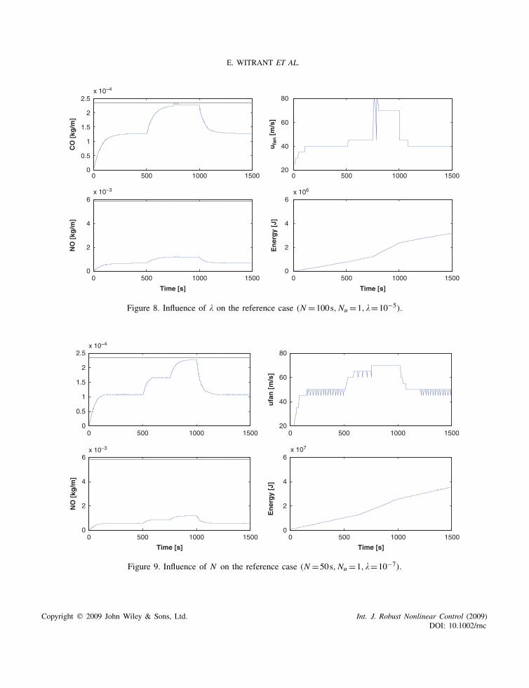
E. WITRANT ET AL.
0 500 1000 15000
0.5
1
1.5
2
2.5
x 106
CO
[kg
/m]
0 500 1000 15000
2
4
6
Time [s]
NO
[kg
/m]
0 500 1000 150020
40
60
80
ufa
n [
m/s
]0 500 1000 1500
0
2
4
6
Time [s]
En
erg
y [J
]
Figure 8. Influence of on the reference case (N =100s,Nu =1,=10−5).
0 500 1000 15000
0.5
1
1.5
2
2.5
0 500 1000 15000
2
4
6
Time [s]
NO
[kg
/m]
0 500 1000 150020
40
60
80
ufa
n [
m/s
]
0 500 1000 15000
2
4
6x 10⁷
Time [s]
En
erg
y [J
]
Figure 9. Influence of N on the reference case (N =50s,Nu =1,=10−7).
Copyright q 2009 John Wiley & Sons, Ltd. Int. J. Robust Nonlinear Control (2009)DOI: 10.1002/rnc

WIRELESS VENTILATION CONTROL
0 500 1000 15000
0.5
1
1.5
2
2.5
0 500 1000 15000
2
4
6
Time [s]
NO
[kg
/m]
0 500 1000 150020
40
60
80
ufa
n [
m/s
]
0 500 1000 15000
2
4
6x 10⁶
Time [s]
En
erg
y [J
]
Figure 10. Influence of Nu on the reference case (N =100s,Nu =2,=10−7).
Remark 2The receding horizon control strategy has proved to beparticularly efficient to achieve optimal performanceson the nonlinear system considered. Communicationconstraints and model uncertainties are easily taken intoaccount and the trade-off between regulation perfor-mance and energy consumption is transparent inthe choice of the scalar parameter . The drawbackis that the high computational demand associatedwith the optimization process may not be appro-priate for embedded applications. This motivates asecond control strategy, presented in the next section,where the algorithm simplicity is preferred to closed-loop performance.
5. HYBRID APPROACH:SAFETY CONTROL STRATEGY
The control strategy proposed in this section is focusedon the safety of the closed-loop system. The secondaryventilation system is modeled conservatively, e.g.using worst-case approximations, and we use a simple
threshold control algorithm. We model the closed-loopsystem using the hybrid systems mathematical frame-work: this allows to take into account the effects oftime-delays, transmission errors and safety constraints.Thus, we use abstraction techniques and tools devel-oped in previous works [35, 36] to verify safety (withrespect to gas concentrations) and temporal propertiesof the system, with a required precision. Since we usea conservative approximation of the original system,if the safety verification algorithm states that theabstract system is safe then the original system is alsosafe.
5.1. Hybrid model
In Section 3.3 we derived the dynamics of the time-dependant shape parameters (t), (t) and (t) in (5)and used them to compute the concentration of gas jat the reference height zr (6). Since such a model cannot be used for the hybrid control approach proposedin this section, we derive approximated (conservative)dynamics for the gas concentration average. We areinterested here in the dynamics of the height-averaged
Copyright q 2009 John Wiley & Sons, Ltd. Int. J. Robust Nonlinear Control (2009)DOI: 10.1002/rnc

E. WITRANT ET AL.
concentration:
C j (h, t).= 1
h
∫ h
0c j (z, t)dz (7)
The pollutant dynamics is simplified by omitting thechemical reactions in the mass conservation law:
m j (t) = m j,in(t)−m j,out(t)
= m j,in(t)+uin(t)Stcatm
−uout(t)SoutC j (hout, t) (8)
where c j,atm is the gas concentration in the atmosphere,Sout is the section of the extraction room output,St is the section of the tarpaulin tube, and uin(t),uout(t)are, respectively, the input and output airflow veloci-ties. Dividing (8) by the room volume VR , we obtainthe concentration dynamics:
C j (hroom,t) = m j,in(t)
VR+ uin(t)Stc j,atm
VR
−uout(t)SoutVR
C j (hout, t) (9)
From the incompressibility hypothesis, (9) can berewritten as
C j (hroom, t) = m j,in(t)
VR+ uin(t)Stc j,atm
VR
−uin(t)StVR
C j (hout, t) (10)
The next step is to simplify the profile descriptionby a rough approximation of the shape parameters. Wecan use a hybrid representation, supposing that j and j can only assume a finite number of constant values
kj and kj , where k is the number of trucks in theroom. In other words, we do not consider the tran-sient dynamics of these parameters when the numberof trucks in the room changes. Note that kj and kjshould also depend on the current airflow velocity atthe room entrance, but we suppose that the strongestcontribution derives from the number of trucks in theextraction room. The dynamics of the average concen-tration in the room is calculated by expressing j (t) as
a function of C j (hroom, t). To this aim, we substitutethe sigmoid function in the integral (7) and obtain:
C j (h, t) = 1
h
∫ h
0
j (t)
1+e−kj (z−kj hroom)dz
= j (t)
kjh
ln
⎛⎝ekj (h−kj hroom)+1
e−kj kj hroom +1
⎞⎠
⇔ j (t) = kj hroom
ln
⎛⎝e
kj (1−kj )hroom +1
e−kj kj hroom +1
⎞⎠C j (hroom, t)
(11)
Substituting (11) in the sigmoid function (c j (z, t)) defi-nition and computing the space averaged concentrationbetween 0 and hout, we have that:
C j (hout, t) = kjhroom
ln
⎛⎝e
kj (1−kj )hroom +1
e−kj kj hroom +1
⎞⎠C j (hroom, t)
× 1
hout
∫ hout
0
1
1+e−kj (−kj hroom)d
Finally, substituting the expression of C j (hout, t) inEquation (10) we obtain:
C j (hroom, t) = m j,in(t)
VR+ uin(t)Sinc j,atm
VR
−uin(t)SinVR
kj hroom
ln
⎛⎝e
kj (1−kj )hroom +1
e−kj kj hroom +1
⎞⎠
×C j (hroom, t)
× 1
hout
∫ hout
0
1
1+e−kj (−kj hroom)d
(12)
Copyright q 2009 John Wiley & Sons, Ltd. Int. J. Robust Nonlinear Control (2009)DOI: 10.1002/rnc

WIRELESS VENTILATION CONTROL
The simplified model for the secondary system is thenthe continuous time non-linear delay system:
C j (hroom, t) = m j,in(t)
VR+ Sinc j,atm
VRufan(t− t (t))
− Sin
VRufan(t− t (t))
×hroom ln
⎛⎝e
kj (hout−kj hroom)+1
e−kj kj hroom +1
⎞⎠
hout ln
(e
kj (1−k)hroom +1
e−kj kj hroom +1
)
×C j (hroom, t) (13)
where t is the worst case delay introduced by thetarpaulin tube tarp(t), as defined in Equation (1). Thedynamics becomes affine if we consider the controlinput ufan piecewise constant (i.e. constant during thesimulation time step) as we will do in the next subsec-tion. Note that depends on the airflow velocity in thetube, due to the Reynolds number dependency.
5.2. Control design
Given the model of the secondary system (13), wedefine the following control specifications.
1. Safety: the gas concentrations cannot enter anunsafe set (a red alert zone), given by standardacceptable air quality for humans.
2. Comfortable air quality: the gas concentrationsmight enter, only for a bounded amount of time,a set (a yellow alert zone) that satisfies safety forhumans, but might be uncomfortable.
These two properties intuitively state the following:we guarantee that the oxygen concentration is alwaysover the minimum safety threshold for humans, and werequire that if a disturbance (e.g. the entrance of a truckin a room) moves it under a threshold of optimality(comfortable air quality), then it only happens for ashort amount of time.
Our aim is to automatically verify whetherthe controlled system satisfies the aforementionedsafety/comfort properties. Thus, we first need to
model the two specifications as formulae. The firststrong specification (classical safety property) can bemodeled using the temporal logic CTL [37], while thesecond relaxed specification can be modeled using thetemporal logic TCTL [38]. Clearly, we have to verifythat both of them are satisfied.
Because of the hybrid nature of the problem (e.g.number of trucks in an extraction room), it is extremelyhard to verify exhaustively on the model (13) whetherthe specifications above are satisfied for any discreteand continuous disturbance. For this reason, wefirst obtain a conservative hybrid model with affinedynamics of our closed-loop system, then construct atimed automaton abstraction of the hybrid automaton,which preserves CTL and TCTL temporal properties.Timed automata can generally be abstracted into finitestate systems [39], which renders the model checkingdecidable.
We now define a hybrid model of our closed-loopsystem with affine dynamics thanks to the followingassumptions.
Assumption 1As a first approach, we consider only two speed levels(which is the case in some of the actual mines, whereonly basic automation is available), namely:
fan∈Lfan, HfanDepending on the maximum gas emission/consumptionof the trucks, we can chose a desired airflow uH
inat the endpoint of the tarpaulin tube and derive the
corresponding fan velocity Hfan using appropriate
engineering data sheet.
Assumption 2A threshold control strategy is considered: we canswitch fans to low and high speed levels when the gasconcentrations hit some given thresholds.
Assumption 3The WSN design guarantees that the measured concen-tration is affected by a bounded estimation error ε>0and that the estimation and communication delays arebounded by a value c>0. As discussed in Section 1,the main wiring problem in the mine is in the extractionroom. Thus, we reasonably assume that the threshold
Copyright q 2009 John Wiley & Sons, Ltd. Int. J. Robust Nonlinear Control (2009)DOI: 10.1002/rnc
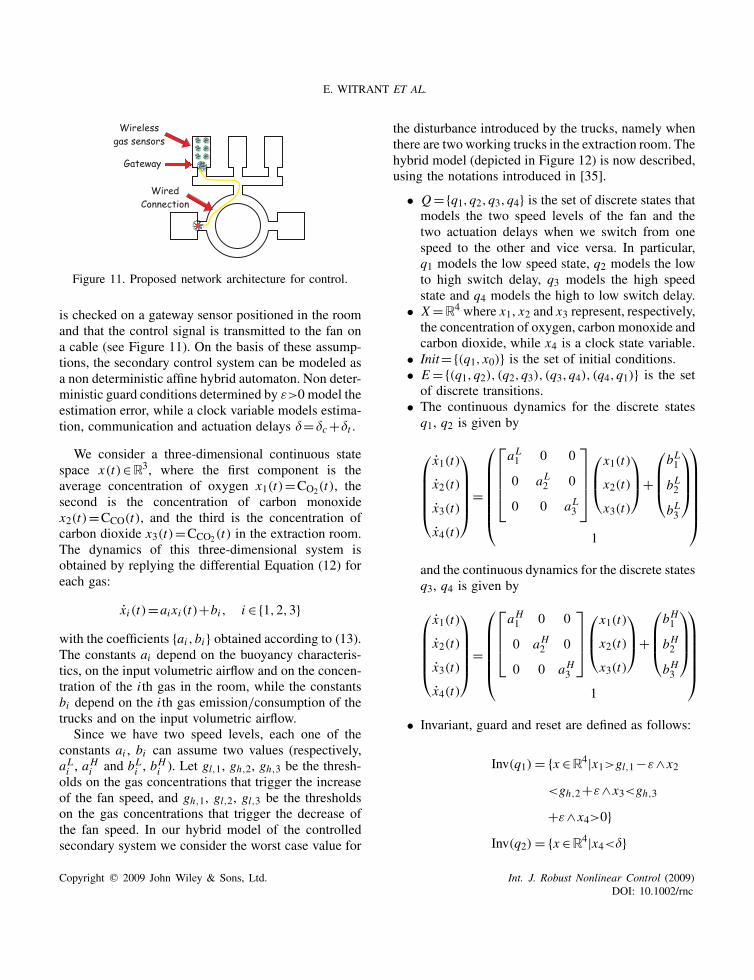
E. WITRANT ET AL.
Figure 11. Proposed network architecture for control.
is checked on a gateway sensor positioned in the roomand that the control signal is transmitted to the fan ona cable (see Figure 11). On the basis of these assump-tions, the secondary control system can be modeled asa non deterministic affine hybrid automaton. Non deter-ministic guard conditions determined by ε>0 model theestimation error, while a clock variable models estima-tion, communication and actuation delays = c+ t .
We consider a three-dimensional continuous statespace x(t)∈R3, where the first component is theaverage concentration of oxygen x1(t)=CO2(t), thesecond is the concentration of carbon monoxidex2(t)=CCO(t), and the third is the concentration ofcarbon dioxide x3(t)=CCO2(t) in the extraction room.The dynamics of this three-dimensional system isobtained by replying the differential Equation (12) foreach gas:
xi (t)=aixi (t)+bi , i ∈1,2,3with the coefficients ai ,bi obtained according to (13).The constants ai depend on the buoyancy characteris-tics, on the input volumetric airflow and on the concen-tration of the i th gas in the room, while the constantsbi depend on the i th gas emission/consumption of thetrucks and on the input volumetric airflow.
Since we have two speed levels, each one of theconstants ai , bi can assume two values (respectively,aLi , a
Hi and bLi , b
Hi ). Let gl,1, gh,2, gh,3 be the thresh-
olds on the gas concentrations that trigger the increaseof the fan speed, and gh,1, gl,2, gl,3 be the thresholdson the gas concentrations that trigger the decrease ofthe fan speed. In our hybrid model of the controlledsecondary system we consider the worst case value for
the disturbance introduced by the trucks, namely whenthere are two working trucks in the extraction room. Thehybrid model (depicted in Figure 12) is now described,using the notations introduced in [35].
• Q=q1,q2,q3,q4 is the set of discrete states thatmodels the two speed levels of the fan and thetwo actuation delays when we switch from onespeed to the other and vice versa. In particular,q1 models the low speed state, q2 models the lowto high switch delay, q3 models the high speedstate and q4 models the high to low switch delay.
• X=R4 where x1, x2 and x3 represent, respectively,the concentration of oxygen, carbon monoxide andcarbon dioxide, while x4 is a clock state variable.
• Init=(q1, x0) is the set of initial conditions.• E=(q1,q2), (q2,q3), (q3,q4), (q4,q1) is the setof discrete transitions.
• The continuous dynamics for the discrete statesq1, q2 is given by
⎛⎜⎜⎜⎜⎝x1(t)
x2(t)
x3(t)
x4(t)
⎞⎟⎟⎟⎟⎠=
⎛⎜⎜⎜⎜⎜⎜⎝
⎡⎢⎢⎢⎣aL1 0 0
0 aL2 0
0 0 aL3
⎤⎥⎥⎥⎦⎛⎜⎝x1(t)
x2(t)
x3(t)
⎞⎟⎠+
⎛⎜⎜⎝bL1
bL2
bL3
⎞⎟⎟⎠
1
⎞⎟⎟⎟⎟⎟⎟⎠
and the continuous dynamics for the discrete statesq3, q4 is given by
⎛⎜⎜⎜⎜⎝x1(t)
x2(t)
x3(t)
x4(t)
⎞⎟⎟⎟⎟⎠=
⎛⎜⎜⎜⎜⎜⎝
⎡⎢⎢⎣aH1 0 0
0 aH2 0
0 0 aH3
⎤⎥⎥⎦⎛⎜⎝x1(t)
x2(t)
x3(t)
⎞⎟⎠+
⎛⎜⎜⎝bH1
bH2
bH3
⎞⎟⎟⎠
1
⎞⎟⎟⎟⎟⎟⎠
• Invariant, guard and reset are defined as follows:
Inv(q1) = x ∈R4|x1>gl,1−ε∧x2
<gh,2+ε∧x3<gh,3
+ε∧x4>0Inv(q2) = x ∈R4|x4<
Copyright q 2009 John Wiley & Sons, Ltd. Int. J. Robust Nonlinear Control (2009)DOI: 10.1002/rnc

WIRELESS VENTILATION CONTROL
Figure 12. Hybrid model of the closed-loop secondary system.
Inv(q3) = x ∈R4|x1<gh,1
+ε∨x2>gl,2−ε∨x3
>gl,3−ε∨x4>0Inv(q4) = x ∈R4|x4<
G(q1,q2) = x ∈R4|x1gl,1
−ε∨x2gh,2
+ε∨x3gh,3+εG(q2,q3) = x ∈R4|x4
G(q3,q4) = x ∈R4|x1gh,1+ε∧x2
gl,2−ε∧x3gl,3−εG(q4,q1) = x ∈R4|x4
∀e∈ E, R(e, x(t)) = (x1(t), x2(t), x3(t),0)′
The threshold control strategy is designed by definingthe guards gl,1, gl,2, gl,3, gh,1, gh,2 and gh,3. We nowautomatically verify, by using the theoretical resultsintroduced in [36] and the tool developed in [35], if fora given control strategy the hybrid automaton definedabove (which models the closed-loop secondary system
Copyright q 2009 John Wiley & Sons, Ltd. Int. J. Robust Nonlinear Control (2009)DOI: 10.1002/rnc

E. WITRANT ET AL.
according to our control strategy) satisfies Safety andComfort properties. More precisely, define the Safetyspecification introduced above as a CTL formula s ,and define the comfortable air quality specification asa TCTL formula c(tmax), where tmax is the maximumtime the system is allowed to dwell in uncomfortableair quality.
Unfortunately, model checking is in general unde-cidable also for affine hybrid automata: an importanttechnique used to cope with complexity is abstraction.In recent papers [35, 36] an algorithm that constructs anabstraction of a hybrid automaton with affine dynamicswas proposed and implemented. Such a algorithmpreserves temporal properties expressed by CTL andTCTL temporal logics. The abstract model belongs to asubclass of timed automata, which is called durationalgraph. Durational graphs are a special class of timedand hybrid automata [40, 41], in which the continuousvariables are clocks, increasing with a constant slope.Resets are restricted to clock resets to 0.
The following result is directly implied by the resultsdeveloped in [36]:Proposition 1Given a hybrid automaton H and a durational graphG such that H and G are bisimilar with precision (H≈G), then:
(i.) If the specification s is satisfied for the systemG, then it is satisfied for the system H.
(ii.) If the specification c(tmax−) is satisfied forthe system G, then c(tmax) is satisfied for thesystem H.
According to the above proposition, we can verify prop-erties of the affine hybrid automaton by checking prop-erties on the durational graph abstraction, using modelchecking tools for timed automata (e.g. KRONOS [42],UPPAAL [43]). If for an initial choice of the thresholdthe system is not verified to be safe, we can iterativelyrun the verification procedure for tighter thresholdsuntil both safety and comfort are satisfied.
The abstraction algorithm’s graphical output isillustrated in Figure 13(a). The algorithm intuitivelyworks as follows. The set of initial conditions of thegas concentrations (blue polytope) is partitioned in afinite number of polytopes according to the continuous
dynamics and the guard sets. The property of eachelement of the partition is that, for each pair of initialconditions x01 , x
02 belonging to it, the arrival times t1, t2
to the guard satisfy |t1− t2|<. This procedure is iter-ated to all guard sets (green and red polytopes) of thehybrid automaton. Each partition element is translatedinto a discrete state of the abstracting durational graph.The resulting durational graph G satisfies H≈G,and thus Proposition 1 holds. Moreover, we can getfrom the precision of our abstraction a measure ofsafety: this can be used to optimize the thresholds byiterative search, in order to guarantee safety with adesired robustness and energy consumption reduction.
By executing the automatic verification procedureon our hybrid model using the thresholds gl,1=0.2955,gl,2=0.510−3, gl,3=0.0885, gh,1=0.2975, gh,2=2.5×10⁻³, gh,3=0.091 (in [kg/m3]) and an abstrac-tion precision =1s, we verified on the abstractionG that s is satisfied, and c(tmax) is satisfied fortmax=61s. Since our abstraction has been constructedwith precision =1s, then Proposition 1 implies that(1) the original is safe and (2) the maximum time ofuncomfortable air quality is bounded by 62 s.
For completeness, we also show in Figure 13(b)some Matlab simulations of the closed-loop system.For the particular initial condition chosen for this simu-lation, safety and air quality can be verified using theplots. The advantage of automatic verification is thatthe same two properties can be verified in one shot forthe whole set of initial conditions, which has infinitecardinality.
6. COMPARISON BETWEENTHE TWO APPROACHES
6.1. Comparison framework
In this section we compare the continuous and thehybrid control strategies on the test case proposed inSection 3.5. The safety thresholds CO=0.000234kgm3
and NO=0.0059kgm3 are considered as strongconstraints, in the sense that the regulated pollutantconcentrations have to remain below these values atany time. The comparison is based on simulationresults, for which we compare regulation efficiency,
Copyright q 2009 John Wiley & Sons, Ltd. Int. J. Robust Nonlinear Control (2009)DOI: 10.1002/rnc

WIRELESS VENTILATION CONTROL
X10-3
4
3.8
3.6
3.4
3.2
3
0.2040.206
0.2080.21
0.212 12
34
5
x10-3COO
2
CO
2
(a)
0 100 200 300 400 5000.294
0.295
0.296
0.297
0.298
0.299
0.3
O2
[kg
/m3 ]
CO
2 [k
g/m
3 ]
0 100 200 300 400 5001
1.005
1.01
1.015
1.02
CO
[kg
/m3 ]
0 100 200 300 400 5000.0879
0.088
0.0881
0.0882
0.0883
Time [s](b)
Figure 13. Matlab simulations and screenshot of the abstraction algorithm output. (a) Polytopes representing the set ofinitial conditions and the projections of their executions with the guard sets and (b) temporal simulation.
energy consumption, robustness with respect to modeluncertainties, and computational complexity.
For comparison consistency, the MPC control lawdepicted in 4.1 is tested with a control regulation objec-tive set to 90% of the thresholds, while for the discretestrategy a choice of the guards gl,CO/NO and gh,CO/NOat 80% and 90% of the safety thresholds is made. Forboth strategies, the high and low operating conditionsof the fans result in flow speeds ufan of 10 and 80m/s,respectively. The parameters for the MPC strategy areset to =10−5, N =100 and Nu =1. Simulation resultsof the two strategies are depicted in Figure 14.
6.2. Regulation efficiency
For both strategies, the safety conditions are satisfied.The MPC is tuned such that both approaches have acomparable energy consumption. We can see that, interms of regulation efficiency, the MPC leads most ofthe time as the pollutant concentration is significantlylower (40% lower for the one truck case, equivalent
when there are two trucks and 12% higher for the threetrucks case).
6.3. Energy Consumption and control input
The energy consumption is compared using the fanmodel discussed in Section 3.4. Figure 14 shows thatthe MPC strategy is more efficient (by approximately8.2%) with respect to energy consumption. This ismainly due to the fact that a relatively high has beenchosen for this comparison, leading to a strong weighton power consumption optimization. Furthermore, theMPC approach obviously leads to smoother controllaws. Note that the observed differences between thetwo approaches are also related to the nonlinear proper-ties of the plant and to the tuning of the controller gains(or choice of the guards for the thresholds approach).
6.4. Robustness with respect to model uncertainties
In the receding horizon strategy, one has to considera prediction model of the system. In our case, the
Copyright q 2009 John Wiley & Sons, Ltd. Int. J. Robust Nonlinear Control (2009)DOI: 10.1002/rnc

E. WITRANT ET AL.
0 500 1000 15000
0.5
1
1.5
2
2.5
0 500 1000 15000
2
4
6
Time [s]
NO
[kg
/m]
0 500 1000 15000
20
40
60
80
ufa
n [
m/s
]
0 500 1000 15000
1
2
3
4x 10⁶
Time [s]
En
erg
y [J
]
Figure 14. Comparison of the two approaches—MPC (solid) and Hybrid (dotted).
prediction model is the reference model, with themaximum time delay, and prediction of pollutantsources at mid value. Feasibility of successive opti-mization problems appears to be a crucial point in thereceding horizon strategy. The constraints are takeninto account by adding some hard penalization terms inthe optimization criterion. Thus, when the constraintsbegin to be slightly violated, the control law increasesits value to satisfy the constraints as soon as possible.More advanced strategies are investigated in [44], butthe previous approach appears to be sufficient for themine ventilation, as illustrated by the robustness testspresented in Figure 15(b).
Two different robustness tests were performed. Inthe first one (Figure 15(a)), we consider underestimatedvalues for the prediction of the pollutant sources. Thus,for this test, the prediction model assumes that there isonly one truck in themine. This is a worst case situation,as can be seen from the real truck profile of Figure 7.The second test (Figure 15(b)) consists of testing a 20%underestimated gain of the system. In other words, the
prediction model assumes that the amount of pollutantis always lower and slower than in reality. Both testsshow that the MPC strategy is robust against pollutantprediction errors and model uncertainties.
While the hybrid approach is structurally robust, inthe sense that it converges in finite time, the thresh-olds may not be satisfied due to the system inertia andneglected dynamics. This can happen, for example, ifwe choose the guards at 85% and 95% of the thresholdvalues, as illustrated in Figure 16. Even if the fans areset to their maximum value once the threshold is trig-gered, the controller cannot predict the safety marginthat is necessary to compensate for the inertia of thepollutants concentration in the room.
6.5. Computational complexity
The computational complexity of the threshold controlstrategy is O(1), namely the control algorithm can beexecuted in a constant (and very short) time. In fact, thecontroller is very simple and does not require any kind
Copyright q 2009 John Wiley & Sons, Ltd. Int. J. Robust Nonlinear Control (2009)DOI: 10.1002/rnc

WIRELESS VENTILATION CONTROL
0 500 1000 15000
0.5
1
1.5
2
2.5
0 500 1000 15000
2
4
6
Time [s]
NO
[kg
/m]
0 500 1000 15000
20
40
60
80
ufa
n [
m/s
]
0 500 1000 15000
2
4
6
Time [s]
En
erg
y [J
]
0 500 1000 15000
0.5
1
1.5
2
2.5
0 500 1000 15000
2
4
6
Time [s]
NO
[kg
/m]
0 500 1000 150020
40
60
80
ufa
n [
m/s
]
0 500 1000 15000
2
4
6
Time [s]
En
erg
y [J
]
(a)
(b)
Figure 15. Robustness tests (N =100s,Nu =1,=10−5): (a) MPC with underestimated pollutant source (1 truck)and (b) MPC with parameter uncertainty.
Copyright q 2009 John Wiley & Sons, Ltd. Int. J. Robust Nonlinear Control (2009)DOI: 10.1002/rnc

E. WITRANT ET AL.
0 500 1000 15000
0.5
1
1.5
2
2.5
0 500 1000 15000
20
40
60
80
u fan
[m/s
]
0 500 1000 15000
2
4
6
NO
[kg/
m]
Time [s]
0 500 1000 15000
1
2
3
4x 10⁶
Ene
rgy
[J]
Time [s]
Figure 16. Threshold control strategy with slightly modified guards.
of computation, since it is based only on the compar-ison between measurements and safety thresholds. Onthe contrary, the MPC approach is computationally timeconsuming, since hard optimization problems have tobe solved at each sampling time. More precisely, theevaluation of the cost function implies the simulation ofthe whole model, as well as the numerical integrationof differential equations. The number of such simula-tions grows exponentially with the number of degreesof freedom Nu in the control law design. Further, in thereal implementation of the MPC control algorithm itis necessary to take into account, before the predictionstage, the reconstruction of those states which param-eterize the finite time optimal control problem to besolved at each sampling period.
Remark 3The comparison between the continuous and the hybridcontrol strategies have shown that the nonlinear modelpredictive control outperforms the safety control,in terms of energy consumption minimization androbustness. This performance is achieved at the price
of a higher computational complexity, which rendersthe MPC difficult to envision for embedded systems,while the threshold control strategy can be included ina modern wireless sensor equipped with a microchip.From an implementation point of view we can thenrelate the choice of the control strategy to the regu-lation architecture presented in Section 2.1. Indeed,if a centralized approach can be implemented, thenthere is no difficulty to set the MPC in the controlroom. If the computational resource is limited to theWSN, then the threshold control strategy can be usedto reduce the energy consumption in comparison withthe actual on/off strategy.
7. CONCLUSIONS
We provided a precise description of the mining venti-lation problem, a novel industrial case in the fieldof control that is of prime environmental importanceand where advanced control methodologies can bringa major improvement. This problem was formulated
Copyright q 2009 John Wiley & Sons, Ltd. Int. J. Robust Nonlinear Control (2009)DOI: 10.1002/rnc
WIRELESS VENTILATION CONTROL
as the one of wireless ventilation control for large-scale systems, the core idea being to combine WSNcapabilities with model-based control strategies. Weconsequently derived a new control-oriented model thatincludes the various dynamics of this multi-physicsprocess. The constraints induced by the WSN weremostly associated with time-delays and packet losses.The modeling of the complete system have shown thatthe communication constraints have a secondary impor-tance compared to the regulated pollutants dynamics.
Two different control approaches were applied:a continuous approach based on a receding horizonscheme (MPC) and a threshold control strategy thatuses a mathematical abstraction of the system. Thefirst approach was shown to allow for a precise controlof the pollution level, explicitly taking into account thenon linearities and operation constraints, and providingfor an easy tuning between closed-loop performanceand energy consumption. The second approach wasfocused on guaranteeing safety and providing fora reduced-complexity regulation that is suitable forembedded control. Comparing the two approaches, itappeared that significantly improved performances canbe achieved thanks to MPC while the threshold controlstrategy can be easily embedded in WSN. Such resultcan be used as an automation design argument, tomotivate a centralized control approach (offering largercomputational capabilities) or to evaluate the gainsassociated with a WSN-embedded control solution.
The on-line estimation of key model parameters andthe design of a new control strategy that can synthe-size the advantages of the two approaches may provideinteresting guidelines for future research.
ACKNOWLEDGEMENTS
The authors greatly acknowledge the contribution of theanonymous reviewers, who significantly participated in thepaper improvement thanks to their thoughtful and construc-tive remarks.
REFERENCES
1. van der Merwe C. Mining industry challenged to cut energyconsumption 15% by 2015. Mining Weekly Online 2007.
2. Xenergy Inc. United States industrial electric motor systemsmarket opportunities assessment, Office of energy efficiency
and renewable energy. Technical Report, U.S. Department ofEnergy, 1998.
3. Scheihing PE, Rosenberg M, Olszewski M, Cockrill C,Oliver J. United States industrial motor-driven systems marketassessment: charting a roadmap to energy savings for industry.International Workshop on Industrial Energy EfficiencyPolicies: Understanding Success and Failure, Utrecht, TheNetherlands, 1998.
4. Hartman HL, Mutmansky JM, Ramani RV, Wang YJ. MineVentilation and Air Conditioning (3rd edn). Wiley: New York,1997.
5. The Second International Conference on WirelessCommunications in Underground and Confined Areas.Val-d’Or, Canada, 2008.
6. Isaksson A, Strand M, Di Benedetto MD, D’Innocenzo A,Santucci F, Serra E, Tennina S, Tiberi U, Bemporad A,Di Cairano S, Maggi F, Synekidou M, D’Angelo M, JohanssonKH, Seuret A, Witrant E, Fischione C. Final report on theindustrial test case. HYCON Deliverable D4d.5.3, 2008.
7. Pomante L, Santucci F, Rinaldi C, Tennina S, FischioneC. Mining ventilation automation: wireless sensing,communication architecture and advanced services. IEEECASE, 2008.
8. Witrant E, D’Innocenzo A, Isaksson A, Di Benedetto M,Johansson K, Santucci F, Strand M. Mining ventilation control:a new industrial case for wireless automation. Proceedings ofthe IEEE Conference on Automation Science and Engineering(CASE 2008), Washington, DC, U.S.A., 2008.
9. Sandou G, Witrant E, Olaru S, Niculescu S. Receding horizonclimate control in metal mine extraction rooms IEEE CASE,2008.
10. Di Benedetto M, D’Innocenzo A, Serra E, Witrant E.Automatic verification of wireless control in a miningventilation system, IEEE CASE’08, 2008.
11. Tolmachev S, Fainshtein E. Analysis of multi-branch junctionsin ventilation networks, regarded as systems with distributedparameters. Journal of Mining Science 1968; 4(2):128–133.
12. Klebanov F, Martynyuk G. A method for experimentaldetermination of the coefficient of longitudinal turbulentdiffusion in ventilating currents of mine workings. Journal ofMining Science 1973; 9(4):413–416.
13. Kalabin G, Baklanov A, Amosov P. Calculating the aerogasdynamics of chamber-like mine workings on the basis ofmathematical modeling. Journal of Mining Science 1990;26(1):61–73.
14. Petrov N, Shishkin M, Dnitriev V, Shadrin V. Modelingmine aerology problems. Journal of Mining Science 1992;28(2):185–191.
15. Petrov N. Methods of solving problems and designingequipment for mine ventilation. Journal of Mining Science1994; 30(2):195–204.
16. Widzyk-Capehart E, Watson B. Agnew gold mine expansionmine ventilation evaluation using VentSim. Proceedings of the7th International Mine Ventilation Congress, 2001.
Copyright q 2009 John Wiley & Sons, Ltd. Int. J. Robust Nonlinear Control (2009)DOI: 10.1002/rnc
E. WITRANT ET AL.
17. Estrin D, Govindan R, Eidemann J, Kumar S. Nextcentury challenges: Scalable coordination in sensor networks.Proceedings of the ACM/IEEE International Conference onMobile Computing and Networking, 1999.
18. Ribeiro A, Giannakis GB. Bandwidth-constrained distributedestimation for wireless sensor networks—part I and II. IEEETransaction on Signal Processing 2006; 54.
19. Witrant E, Johansson K. The HynX team. Air flow modellingin deep wells: application to mining ventilation. IEEE CASE,2008.
20. Schmidt W. Turbulent propagation of a stream of heated air.Zeitschrift fur Angewandte Mathematik and Mechanik 1941;21:265–278, 351–363.
21. Morton B. Forced plumes. Journal of Fluid Mechanics 1959;5(1):151–163.
22. Liu Q, Linden P. The fluid dynamics of an underfloorair distribution system. Journal of Fluid Mechanics 2006;554:323–341.
23. Hirsch C. Numerical Computation of Internal & ExternalFlows: The Fundamentals of Computational Fluid Dynamics.(2nd edn). Butterworth-Heinemann (Elsevier): London, 2007.
24. Park PG. Randomized protocol design in wireless automation.M. Eng. Thesis, Royal Institute of Technology (KTH),Stockholm, Sweden, 2007.
25. Witrant E, Park PG, Johansson M, Johansson K, Fischione C.Control over wireless multi-hop networks. Proceedings of theIEEE Conference on Control Applications, 2007.
26. Lee P, Garimella S, Liu D. Investigation of heat transfer inrectangular microchannels. International Journal of Heat andMass Transfer 2005; 48:1688–1704.
27. Witrant E, Joffrin E, Bremond S, Giruzzi G, Mazon D,Barana O, Moreau P. A control-oriented model of the currentprofile in tokamak plasma. Plasma Physics Controlled Fusion2007; 49:1075–1105.
28. Ljung L. System Identification: Theory for the User (2nd edn).Prentice-Hall PTR: Englewood Cliffs, NJ, 1998.
29. Nerguizian C, Despins C, Affes S. Geolocation in mineswith an impulse response fingerprinting technique and neuralnetworks. IEEE Transactions on Wireless Communications2006; 5(3).
30. Chehri A, Fortier P, Tardif P-M. Frequency domain analysisof UWB channel propagation in underground mines. 64thIEEE Conference on Vehicular Technology, 2006.
31. Krause P. Analysis of Electrical Machinery. McGraw-Hill:New York, 1986.
32. Frey H, Kim K. Comparison of real-world fuel use andemissions for dump trucks fueled with B20 biodiesel versuspetroleum diesel. 85th Annual Meeting of the TransportationResearch Board, 2006.
33. Maciejowski J. Predictive Control with Constraints. Prentice-Hall: Englewood Cliffs, NJ, 2002.
34. Mayne DQ, Rawlings JB, Rao C, Scokaert P. Constrainedmodel predictive control: stability and optimality. Automatica2000; 30:789–814.
35. D’Innocenzo A, Julius AA, Pappas GJ, Di Benedetto MD,Di Gennaro S. Verification of temporal properties on hybridautomata by simulation relations. Proceedings of the 46thIEEE Conference on Decision and Control, New Orleans,U.S.A., 2007.
36. D’Innocenzo A, Julius A, Di Benedetto M, PappasG. Approximate timed abstractions of hybrid automata.Proceedings of the 46th IEEE Conference on Decision andControl. New Orleans, Louisiana, U.S.A., 2007.
37. Clarke E, Grumberg O, Peled D. Model Checking. The MITPress: Cambridge, MA, 2002.
38. Alur R, Courcoubetis C, Dill D, Model-checking in densereal-time. Information and Computation 1993 104(1):2–34.
39. Alur R, Henzinger T, Lafferriere G, Pappas G. Discreteabstractions of hybrid systems. Proccedings of the IEEE 2000;88(2):971–984.
40. Alur R, Dill D. A theory of timed automata. TheoreticalComputer Science 1994; 126:183–235.
41. Alur R, Courcoubetis C, Halbwachs N, Henzinger T, Ho P,Nicollin X, Olivero A, Sifakis J, Yovine S. The algorithmicanalysis of hybrid systems. Theoretical Computer Science1995; 138:3–34.
42. Yovine S. Kronos: a verification tool for real-time systems.International Journal of Software Tools for TechnologyTransfer 1997 1(1):123–133.
43. Larsen KG, Pettersson P, Yi W. UPPAAL in a nutshell.International Journal on Software Tools for TechnologyTransfer 1997; 1(1):134–152.
44. Sandou G, Olaru S. Hybrid systems computation and control.Ant Colony and Genetic Algorithm for Constrained PredictiveControl of Power Systems. Lecture Notes in Computer Science,vol. 4416. Springer: Berlin, Heidelberg, 2007; 501–514.
Copyright q 2009 John Wiley & Sons, Ltd. Int. J. Robust Nonlinear Control (2009)DOI: 10.1002/rnc
June 29, 2007 14:38 International Journal of Systems Science IJSS
International Journal of Systems ScienceVol. 00, No. 00, January 2005, 1–29
Multivariable torque tracking control for E-IVT hybridpowertrain
O. REYSS†§, G. DUC§, P. POGNANT-GROS† and G. SANDOU§
§ Automatic Control Department, École supérieure d’électricité,3 rue Joliot Curie, 91192 Gif-Sur-Yvette, France† Renault Advanced Engineering Department,avenue du golf, 78288 Guyancourt, France
(Received 00 Month 200x; In final form 00 Month 200x)
This study deals with the control of an hybrid vehicle powertrain, composed of three actuators (oneengine, two electric machines). This powertrain belongs to the Electric-Infinitely Variable Trans-mission (E-IVT) class. In order to achieve low fuel consumption, drivability and electric powermanagement, controllers must achieve simultaneously three specifications: tracking engine speed,wheel-torque and battery power references. Decoupled controlled-output behaviors and maximalperformances are also required.In order to imitate a classical powertrain control structure, the control structure is split in two parts.The interest is to decouple transmission speed ratio control and wheel torque control. A model-baseddesign approach is proposed, that directly deals with robustness and decoupling, in a full multivari-able and frequency-dependent framework (H∞ synthesis).Closed-loop simulations are presented. Stability and performances face to disturbances and non-linearities are also evaluated, using the theory of linear parameter varying systems.
Keywords: H∞-synthesis; Linear Parameter Varying Systems; Hybrid electricpowertrain.
1 Introduction
The development of new automotive engine and powertrain concepts is drivenby the aim to reduce the average fleet CO2 emissions and fuel consumption.Hybrid powertrain concepts, in addition to the conventional internal combus-tion engine, are equipped with one or more electrical machines and a batteryas an energy storage unit. By using the specific advantages of both powersources, hybrid vehicles are considered as a short term possibility to achievethe mentioned goals.
Corresponding author. Email: [email protected]

June 29, 2007 14:38 International Journal of Systems Science IJSS
2 Multivariable torque tracking control for E-IVT hybrid powertrain
In the frame of an Advanced Engineering Department project, RENAULThas initiated collaboration with the Automatic Control Department of SUP-ELEC. The study deals with the control of a dual-mode power-split hybridpowertrain. Such a transmission is composed of three actuators (one internalcombustion engine, two electric machines) which allow managing the powerfrom the engine and the battery to the wheels. Opening or closing clutchesand breaks change speed ratios between actuators and wheels, so we have twodifferent mechanical modes. In order to achieve low fuel consumption, driv-ability and electric power management, main control specifications are: track-ing engine speed, wheel torque and battery power references, decoupling thecontrolled-output behaviors and achieving maximal closed-loop performancesfaced to uncertainties or non-linearities. This powertrain is described in section2.
To enable the design of the control law, a complete model of the system hasbeen defined. Its study showed that it is possible to perform reduction withoutlosing accuracy on its behavior. It also showed non-linearities due to batterycharge process. Indeed, our system can be written as a quasi-LPV model (linearparameter varying), which means that matrices of its state-space descriptionare time-varying. Although stability and performances of our system couldseriously be degraded by this non-linearity, a linear time invariant controllerhas been designed. As a result, the stability and performance robustness faceto such variations will have to be guaranteed.
In order to imitate a classical powertrain control behavior, the control struc-ture has been split in two parts. The interest is to decouple transmission speedratio control and wheel torque control. As shown in section 3, this new controllaw is composed of two controllers : a 2×2-multivariable part, controlling inter-nal combustion engine speed and battery power from electric machine torques,and an open-loop part, controlling wheel torque from the internal combustionengine. To design the closed-loop part of the control structure, a model-baseddesign approach was proposed, that directly deals with robustness and decou-pling, in a full multivariable and frequency-dependent framework. It is basedon H∞ synthesis. Many specifications have to be taken into account, suchas reaching performances, respecting actuators limitations and stability mar-gins, and rejecting disturbances. All these specifications can be expressed byfrequency-dependent weights on different closed-loop transfers. This approachallows fixing compromises between each closed-loop objectives and is presentedin section 4.
Robust stability and performances face to disturbances and non-linearitieshave been analysed in section 5. This part of the study was first axed on theanalysis of the linearised system, using µ-analysis. Stability and performances

June 29, 2007 14:38 International Journal of Systems Science IJSS
O. REYSS, G. DUC, P. POGNANT-GROS and G. SANDOU 3
of the non-linear system have then been analysed by applying the LPV systemstheory. Each method gave good results. Closed-loop simulations on a model ofthe vehicle have been performed. This full model includes actuators or vehiclespeed limits, delays and losses. Since the results detailed in section 6 are veryconvincing, this control law should be implemented into a prototype.
2 System description
2.1 Structure
2.1.1 Mechanical structure. The main advantage of this structure is thepossibility to operate in two mechanical modes. The first one stands for lowspeeds, the second for high speeds. On the other hand, different driving con-ditions imply different control strategies. For example, it may be interestingto track the wheel torque (as a classic car does), whereas it may be better tokeep the engine speed at zero in particular situations. In this study, the firstmechanical mode (low speeds) and the torque tracking strategy will only beconsidered. This structure is presented in Villeneuve (2004).
Figure 1 presents the transmission architecture, operating in the first mode.On this scheme:
• Te1 and ωe1 (respectively Te2 et ωe2) stand for machine 1 (resp. 2) torqueand speed,
• Tice and ωice stand for the torque and speed of the Internal CombustionEngine (ICE),
• Tdwh and ωwh stand for wheel torque and speed,• ki (respectively ko) is the stiffness of the axle that links the ICE to the
powertrain (resp. the axle that links the wheels to the powertrain),• Ti and ωi stand for the torque and speed of the axle that links the ICE to
the powertrain,• To and ωo stand for the torque and speed of the axle that links the wheels
to the powertrain,• Tvi and ωvi stand the torque and speed of the axle that links the electric
machine 1 to the powertrain,• Tvo and ωvo stand for the torque and speed of the axle that links the electric
machine 2 to the powertrain,• Ucapa stands for electric machines input voltage,• Ubatt stands for battery voltage.

June 29, 2007 14:38 International Journal of Systems Science IJSS
4 Multivariable torque tracking control for E-IVT hybrid powertrain
Figure 1. Mechanical structure of the system
In this paper, we will also consider:
• Jice, Jaxle et Je inertias of the ICE, the wheels and electric machines,• Ecapa the battery charge level,• Cx the aerodynamical coefficient of the vehicle,• ρ the air relative density,• Vvh the vehicle speed,• Rwheel the wheel radius,• mvehicle the vehicle weight,• Troad/wheel the torque applied to the wheel by the floor.
According to figure 1, the kinetic part of the powertrain is composed of four

June 29, 2007 14:38 International Journal of Systems Science IJSS
O. REYSS, G. DUC, P. POGNANT-GROS and G. SANDOU 5
planetary trains (1, 2, B and C), two breaks B1 and B2, and four speed ratiosKi, Ko, Kvi and Kvo. This part is connected to the internal combustion engine(ICE), to the wheels and to the electric machines 1 and 2.
The electrotechnical part of the powertrain operates as follow : both ma-chines are connected to a buffer-capacitor via two convertors. The aim of thiscapacitor is not power storage but to ensure a convenient voltage at the ma-chines input. A super-capacitor stands for power storage. Both capacitors areconnected by a step-up DC/DC converter. The high bandwidth of the electricmachines allows us to control the buffer-capacitor voltage using them. Studyingthe transmission behavior, it is possible to only consider the buffer-capacitor,and the super-capacitor and the DC/DC converter can be seen as positive ornegative power stream.
2.1.2 Control structure. To control such a complex system, it is possibleto opt for a multi-level control strategy (see figure 2). Each level has differentaims, different time response and different operating means. Such a leveledapproach is versatile and could be applied to other hybrid vehicles.
Figure 2. leveled control structure
This paper will only deal with one level called the COS (Co-OrdinatingStrategies). Its inputs are references for the wheel torque T ]
o , the ICE speedω]
ice and the electric machines power E]capa. Its aim is to track these references
by generating control inputs (Te1, Te2 and Tice) for both electric machines andfor the ICE.

June 29, 2007 14:38 International Journal of Systems Science IJSS
6 Multivariable torque tracking control for E-IVT hybrid powertrain
2.1.3 Specifications for first mechanical mode - torque tracking. In orderto design a controller for the system, the set of specifications for the firstmechanical mode and the torque tracking strategy is as follows :
(i) time response (τωice) smaller than a predetermined value for ωice;(ii) time response (τωice) smaller than a predetermined value for To;(iii) Ucapa in a range centered on its nominal value U ref
capa;(iv) good stability margins;(v) reduced actuators activity;(vi) controlled-output behaviors decoupling;(vii) rejection of the main disturbances (Tdice, Tdwh et Pdcdc).
2.2 Full and reduced-order models
2.2.1 7 state model. It is possible to get simple equations describing thebehavior of each component of the powertrain :
Internal Combustion Engine (crankshaft):
Jiceωice = Tice − Ti + Tdice
Tdice stands for the friction torque (as well as disturbances on the ICE shaft).
Flywheel:
Ti = ki(ωice − ωi)
Electric machines 1 and 2:
Je
[ωe1
ωe2
]=
[Te1
Te2
]−
[Tvi
Tvo
]
Wheel (one equation for its inertia, one for the shaft stiffness):
To = ko(ωwh − ωo)
Jaxleωwh = −To + Troad/wheel
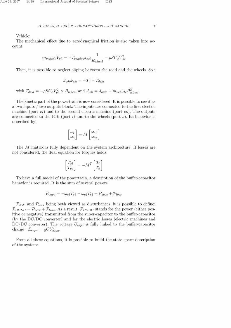
June 29, 2007 14:38 International Journal of Systems Science IJSS
O. REYSS, G. DUC, P. POGNANT-GROS and G. SANDOU 7
Vehicle:The mechanical effect due to aerodynamical friction is also taken into ac-
count:
mvehicleVvh = −Troad/wheel1
Rwheel− ρSCxV 2
vh
Then, it is possible to neglect sliping between the road and the wheels. So :
Jwhωwh = −To + Tdwh
with Tdwh = −ρSCxV 2vh ×Rwheel and Jwh = Jaxle + mvehicleR
2wheel.
The kinetic part of the powertrain is now considered. It is possible to see it asa two inputs / two outputs block. The inputs are connected to the first electricmachine (port vi) and to the second electric machine (port vo). The outputsare connected to the ICE (port i) and to the wheels (port o). Its behavior isdescribed by:
[ωi
ωo
]= M
[ωe1
ωe2
]
The M matrix is fully dependent on the system architecture. If losses arenot considered, the dual equation for torques holds:
[Tvi
Tvo
]= −MT
[Ti
To
]
To have a full model of the powertrain, a description of the buffer-capacitorbehavior is required. It is the sum of several powers:
Ecapa = −ωe1Te1 − ωe2Te2 + Pdcdc + Ploss
Pdcdc and Ploss being both viewed as disturbances, it is possible to define:PDCDC = Pdcdc +Ploss. As a result, PDCDC stands for the power (either pos-itive or negative) transmitted from the super-capacitor to the buffer-capacitor(by the DC/DC converter) and for the electric losses (electric machines andDC/DC converter). The voltage Ucapa is fully linked to the buffer-capacitorcharge : Ecapa = 1
2CU2capa.
From all these equations, it is possible to build the state space descriptionof the system:

June 29, 2007 14:38 International Journal of Systems Science IJSS
8 Multivariable torque tracking control for E-IVT hybrid powertrain
X =
− biceJice
0 0 0 − 1Jice
0 0
0 − bwhJwh
0 0 0 − 1Jwh
0
0 0 0 0J−1
e MT 00 0 0 0 0ki 0 −
[ki 00 ko
]M
0 0 00 ko 0 0 00 0 0 0 0 0 0
X +
0 0 1Jice
0 0 0
J−1e
00
0 0 00 0 0
−ωe1 −ωe2 0
Te1
Te2
Tice
+ (1)
+
1Jice
0 0
0 1Jwh
0
0 0 00 0 00 0 00 0 00 0 1
Tdice
Tdwh
PDCDC
Y =
ωice
To
Ecapa
=
1 0 0 0 0 0 00 0 0 0 0 1 00 0 0 0 0 0 1
X
where the state vector is:
X =[ωice ωwh ωe1 ωe2 Ti To Ecapa
]T
2.2.2 Reduced 3 state model. This 7 state model is a component-basedone. Its study shows that it is possible to reduce the mechanical part to get a3 states model. The mechanical part of the system corresponds to the first 6state of its state-space description. A method to perform such a reduction is toneglect high-frequency dynamics of our system. These dynamics describe thestiffness of shafts (the flywheel and the shaft between the kinetic part and thewheels). Bode diagrams show that the behavior of the full and reduced models,are close on a frequency range from 0 to 10rad.s−1. These diagrams are shownon figure 3. The state space description of the reduced system is as follows:
ωe1
ωe2
Ecapa
= 03×3
[ωe1
ωe2
Ecapa
]+
[M1
−ωe1 −ωe2 0
] [Te1
Te2
Tice
]+ M2
[Tdice
Tdwh
Pdcdc
](2)
[ωice
To
Ecapa
]= M3
[ωe1
ωe2
Ecapa
]+ M4
[Te1
Te2
Tice
]+ M5
[Tdice
Tdwh
Pdcdc
]
where:
M1 = Je−1
[MT
[0 0 10 0 0
]+
[1 0 00 1 0
]]

June 29, 2007 14:38 International Journal of Systems Science IJSS
O. REYSS, G. DUC, P. POGNANT-GROS and G. SANDOU 9
M2 =
[Je−1
MT 00
0 0 1
]
M3 =
[ [ 1 0 ]M 00 0 00 0 1
]
M4 =
01×3
[ 0 1 ] M−T
[JeJe
−1[MT
[0 0 10 0 0
]+
[1 0 00 1 0
]]−
[1 0 00 1 0
]]
01×3
M5 =
01×3
[ 0 1 ] M−T JeJe−1
MT 001×3
with Je = Je + MT
[Jice 00 Jwh
]M .
Figure 3. Full model (solid) and reduced model (dashed) Bode diagrams

June 29, 2007 14:38 International Journal of Systems Science IJSS
10 Multivariable torque tracking control for E-IVT hybrid powertrain
As a result, three disturbances in the reduced model have to be considered:Tdice, Tdwh and PDCDC for the energetic part.
2.3 System properties
The equation describing the energetic part of the system contains torque /speed products. These makes the system being non-linear. In fact, ωe1 and ωe2
are both states and coefficients of the control input matrix of the state spacedescription (see (2)).
A LPV (linear parameter varying) system is a linear system whose statespace description matrices depend on varying parameters. The system (2) isnot exactly a LPV system : one matrix is linearly dependent on ωe1 and ωe2, butthese parameters are also states of the system. Such systems are called quasi-LPV systems. It is possible to find a LPV system that is very close to a quasi-LPV, called an equivalent LPV system. In order to get this system, varyingparameters are replaced by fictive parameters having the same variation rangeand dynamics. Using this method, ωe1 and ωe2 are both considered as statevariables and varying parameters.
Helmersson (1995) and Leith et al. (2000) show that properties satisfiedby the equivalent LPV system are satisfied by the quasi-LPV system (butthe converse is not true). As soon as we consider arbitrarily variation for theequivalent LPV, variations of the states ωe1 and ωe2 are a subset of variationsof the equivalent LPV parameters. It means that tools developed for LPVsystems can be applied to the system, although it is somewhat conservative.
3 COS structure
3.1 Global COS structure
It is possible to describe the COS as a MIMO controller, whose inputs are ref-erences T ]
o , ω]ice and P ]
elec, and each measure delivered by the system, that is to
say Ecapa, ωe1 and ωe2. It is possible to compute ωice as ωice =[1 0
]M
[ωe1
ωe2
]
and to ensure the feedback of each variable (ωice and Ecapa, see figure 4).

June 29, 2007 14:38 International Journal of Systems Science IJSS
O. REYSS, G. DUC, P. POGNANT-GROS and G. SANDOU 11
Figure 4. Classic COS structure
3.2 Structure proposal for the COS
The strategy of figure 4 is fully multivariable. As a result, this control lawmay be totally different from the one used in a classic vehicle, that is splitin two independent but communicating parts: one that tracks the speed ratiobetween the ICE and the wheels (gear box control) and another that tracksthe wheel torque (ICE control). Usually, a mechanic gear box operates in adiscrete mode, but when the car is taking off, its behavior is close to an IVT’sone (so does a robotized gear box changing its speed ratio). Indeed, the gearbox controller or the driver continuously operates on the speed ratio with theclutch. We would like to get profit of such a knowledge by designing a twolevels control structure: a first level tracking the wheel torque by calculatingthe ICE torque, and a second one tracking the speed ratio between the ICEand the wheels, with the two electric machines torques.
The study of the system model (2) shows an interesting property. Since thesecond line of matrix M3 is zero, a simple algebraic equation links six torques: To, Te1, Te2, Tice, Tdice and Tdwh.
Such an equation has important consequences on the control law. It showsthat it is possible to have a first controller K1 for ωice and Ecapa whose outputsare Te1 and Te2, and a second one K2 tracking To using Tice. For the controllaw to be accurate, T ]
o is considered as a disturbance in the design of the thefirst controller. The structure of this control law is described in figure 5.
Consider the reduced model (2), which can be stated as:
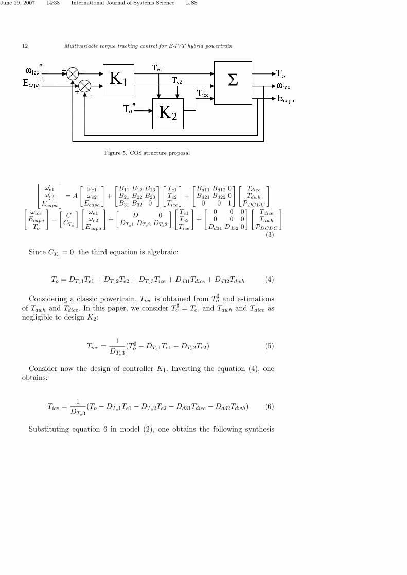
June 29, 2007 14:38 International Journal of Systems Science IJSS
12 Multivariable torque tracking control for E-IVT hybrid powertrain
Figure 5. COS structure proposal
˙ωe1
˙ωe2˙Ecapa
= A
[ωe1
ωe2
Ecapa
]+
[B11 B12 B13
B21 B22 B23
B31 B32 0
][Te1
Te2
Tice
]+
[Bd11 Bd12 0Bd21 Bd22 0
0 0 1
][Tdice
Tdwh
PDCDC
]
[ωice
Ecapa
To
]=
[C
CTo
][ωe1
ωe2
Ecapa
]+
[D 0
DTo1 DTo2 DTo3
] [Te1
Te2
Tice
]+
[ 0 0 00 0 0
Dd31 Dd32 0
][Tdice
Tdwh
PDCDC
]
(3)
Since CTo= 0, the third equation is algebraic:
To = DTo1Te1 + DTo2Te2 + DTo3Tice + Dd31Tdice + Dd32Tdwh (4)
Considering a classic powertrain, Tice is obtained from T ]o and estimations
of Tdwh and Tdice. In this paper, we consider T ]o = To, and Tdwh and Tdice as
negligible to design K2:
Tice =1
DTo3(T ]
o −DTo1Te1 −DTo2Te2) (5)
Consider now the design of controller K1. Inverting the equation (4), oneobtains:
Tice =1
DTo3(To −DTo1Te1 −DTo2Te2 −Dd31Tdice −Dd32Tdwh) (6)
Substituting equation 6 in model (2), one obtains the following synthesis

June 29, 2007 14:38 International Journal of Systems Science IJSS
O. REYSS, G. DUC, P. POGNANT-GROS and G. SANDOU 13
model:
˙ωe1
˙ωe2˙Ecapa
= A
ωe1
ωe2
Ecapa
+ B′
[Te1
Te2
]+ B′
d
Tdice
Tdwh
PDCDC
To
[ωice
Ecapa
]= C
ωe1
ωe2
Ecapa
+ D
[Te1
Te2
](7)
with:
B′ =
B11 −B13DTo1
DTo3B12 −B13
DTo2
DTo3
B21 −B23DTo1
DTo3B22 −B23
DTo2
DTo3
B31 B32
and:
B′d =
Bd11 −B13Dd31DTo3
Bd12 −B13Dd32DTo3
0 B13DTo3
Bd21 −B23Dd31DTo3
Bd22 −B23Dd32DTo3
0 B23DTo3
0 0 1 0
Controller K1 can now be designed by any automatic control method. Themain advantage of this structure is the decoupling of two different behaviors:one part of the control law acts as a gear box controller and controls the batterycharge, the other part as an ICE controller. As explained before, such a controllaw allows using the knowledge of classic powertrains. Furthermore, it may bevery efficient because fast actuators (electric machines) are split from the slowone (ICE).
4 K1 controller synthesis
4.1 Frequency dependent specifications
Sharp specifications are very important to design controllers. It is possible totranslate these specifications into frequency-dependent weights on significant

June 29, 2007 14:38 International Journal of Systems Science IJSS
14 Multivariable torque tracking control for E-IVT hybrid powertrain
transfers. Figure 6 shows the closed-loop system we have to study in order todesign controller K1.
Figure 6. closed-loop system
Studying such a system, most significant transfers are between referencesand disturbances, to tracking errors and control inputs. Thus :
[εu
]=
[S −SG′
K1S −K1SG′
] [rd
]
where : ε = [εωiceεEcapa
]T , u = [Te1 Te2]T , r = [ω]ice E]
capa]T and d =[Tdice Tdwh PDCDC To]T . G and G’ are the transfer function of Σ and Σ′, andS = (I + GK1) is the sensitivity function.
Translating specifications into frequency-dependent weights on these trans-fers gives relevant results. For example, it is possible to reduce the time responseand the tracking errors by ensuring low values for S(jω) at low frequencies,and to reduce actuators activity by reducing K1(jω)S(jω). Low values for−S(jω)G′(jω) and −K1(jω)S(jω)G′(jω) mean high disturbance rejection.
Controller design methods sometimes work with frequency-dependentweights as specifications. This approach allows independently working on eachtransfers and on well defined frequency ranges. This is one of the advantagesof H∞-synthesis.

June 29, 2007 14:38 International Journal of Systems Science IJSS
O. REYSS, G. DUC, P. POGNANT-GROS and G. SANDOU 15
4.2 H∞ synthesis
4.2.1 Principle. The principle of this method is the minimization of the H∞norm of one or several transfers of the system. Such a method allows satisfyingspecifications as: performances (time response, overshoot), stability margins oractuator limitations, by introducing frequency dependent weights, according tothe specifications. These weights are shown on figure 7.
Figure 7. Closed-loop system with frequency dependent weights
Transfers between references and disturbances, and tracking errors and con-trol inputs then become:
[e1
e2
]=
[w1S −w1SG′w3
w2K1S −w1K1SG′w3
] [rd
]
If we perform H∞ synthesis on this model, interesting properties can becaptured. Let’s consider that the obtained controller ensures an H∞ norm ofthe closed-loop system less or equal to γ:
‖[
w1S −w1SG′w3
w2K1S −w1K1SG′w3
]‖∞ ≤ γ

June 29, 2007 14:38 International Journal of Systems Science IJSS
16 Multivariable torque tracking control for E-IVT hybrid powertrain
For a SISO plant, this inequality implies the following properties, ∀ω:
|S(jω)| ≤ γ
|w1(jω)|
|K1(jω)S(jω)| ≤ γ
|w2(jω)|
|S(jω)G′(jω)| ≤ γ
|w1(jω)w3(jω)|
|K1SG′(jω)| ≤ γ
|w2(jω)w3(jω)|
This is an important result because it shows that it is possible to shape eachtransfer by choosing the three weights. For MIMO plants, these inequalitiesfurther hold by using singular values, or by considering each particular SISOtransfer. It is therefore possible to have sharp specifications on each reference(with w1), each control input (w2) and each disturbance (w3). Note that spec-ifications are satisfied only if γ ≤ 1.
It is important to consider two things. First, transfers are not equal to the fre-quency dependent weights, they only satisfy the inequalities. Then, the harderthe specifications are, the bigger is γ (remember that specifications are onlysatisfied if γ ≤ 1). Performing such methods, the most difficult thing is to get asuitable compromise between each specification and system limits. This choiceis often made by proceeding iterative shaping of the weights.
Two methods are mostly used to perform H∞ synthesis: they are based onsolving Riccati equations (see Doyle et al. (1989), Glover et al. (1988) and Zhouet al. (1996) and LMIs (linear matrix inequalities, see Apkarian et al. (1994)).

June 29, 2007 14:38 International Journal of Systems Science IJSS
O. REYSS, G. DUC, P. POGNANT-GROS and G. SANDOU 17
4.3 Variations of ωe1 and ωe2
4.3.1 Polytope. One matrix of the state space description of the system islinearly dependent on ωe1 and ωe2. As a result, ωe1 and ωe2 being also statevariables, the system is a quasi-LPV one. As explained before, it is possible tostudy these systems as LPVs, by considering ωe1 and ωe2 both as state vari-ables and varying parameters. Furthermore, since the plant matrices linearlydepend on ωe1 and ωe2, a polytopic LPV representation can be used: such anapproach requires considering that ωe1 and ωe2 evolve in a convex polygoneof R2, which is called a polytope. It will be defined by considering differentphysical limitations, the first one being the variation ranges [ωe1min; ωe1max]and [ωe2min; ωe2max].
In a simple model of the system (neglecting stiffness of the flywheel and theaxles), there is an algebraic relation linking ωe1, ωe2, ωice and ωwh (so doesthe vehicle speed Vvh). The matrix that links these variables is M . There arelimitations on ωice and Vvh too.
The main difference between both mechanical modes is the value of M . Onthe other hand, the first mechanical mode stands for ωe1 > 0, and the secondmode stands for ωe1 < 0. It is possible to draw the two polytopes (for eachmode) on the same figure.
Taking into account all limitations gives the domain represented on figure 8.The biggest square stands for the electric machines limitations, dotted areasrepresent ωice and Vvh limitations and A, B, C and D areas are the intersectionsof both. As we are studying the first mechanical mode, we only consider thepolytope obtained by the union of zones A and B.
4.3.2 Controllability and observability. The study of the system control-lability and observability is necessary before designing a controller. In fact, itis necessary to know if these properties are satisfied on the whole polytope.Here, consider the reduced model used for the controller K1 synthesis (withonly two outputs, see (7)). It is possible to show that the system controllabilityvanishes on a line satisfying:
ωe2
ωe1= −M(1, 1)
M(1, 2)

June 29, 2007 14:38 International Journal of Systems Science IJSS
18 Multivariable torque tracking control for E-IVT hybrid powertrain
Figure 8. ωe1 and ωe2 polytope, taking all limitations into account
In fact, on this line, two columns of the state space description of the systembecome proportional. However, as this line is outside the polytope, we can saythat controllability and observability conditions are convenient in the wholepolytope.
5 LTI controller - H∞ synthesis
5.1 Synthesis framework
The system being an LPV, it is possible to design either a non-linear controller(for example a polytopic LPV controller) or a LTI controller. The choice thatis made in this paper, is to design a LTI controller based on the model lin-earised on a significant operating point of the polytope. To validate this choice,stability and performances of such a controller have to be analysed with LPV

June 29, 2007 14:38 International Journal of Systems Science IJSS
O. REYSS, G. DUC, P. POGNANT-GROS and G. SANDOU 19
analysis tools.
According to this, conditions to perform the synthesis of a robust controllerare:
(i) consider a two levels control structure,(ii) focus on the first mechanical mode, and a torque tracking strategy,(iii) use a linearised model of the system for some operating point,(iv) perform H∞ synthesis,(v) design frequency dependent weights induced by specifications:
Two first order weights are introduced for tracking errors and control inputs,whereas w3(s) is chosen as a constant diagonal matrix:
w1(s) =
[Ko11Kinf11s+Ko11ωc11
Ko11s+ωc110
0 Ko12Kinf12s+Ko12ωc12
Ko12s+ωc12
]
w2(s) =
1ωc2
s+Ko2
1Kinf2ωc2
s+10
01
ωc2s+Ko2
1Kinf2ωc2
s+1
w3(s) =
K31 0 0 00 K32 0 00 0 K33 00 0 0 K34
where Ko11, Ko12 and Ko2 stand for low frequency gains, Kinf11, Kinf12
and Kinf2 stand for high frequency gains and ωc11, ωc12 and ωc2 are the 0dBcrossover frequencies. K31, K32, K33 and K34 are constant gains.
Roughly speaking, Ko11, Ko12 have to be high enough to obtain zero steady-state errors; Kinf11, Kinf12 are less than 1 and control the stability margins;ωc11, ωc12 allow tuning the bandwidth; Ko2 is less than 1 while Kinf2 (greaterthan 1) together with ωc2 allow reducing the actuators’ activity; finally gainsK3i allow disturbance rejection.
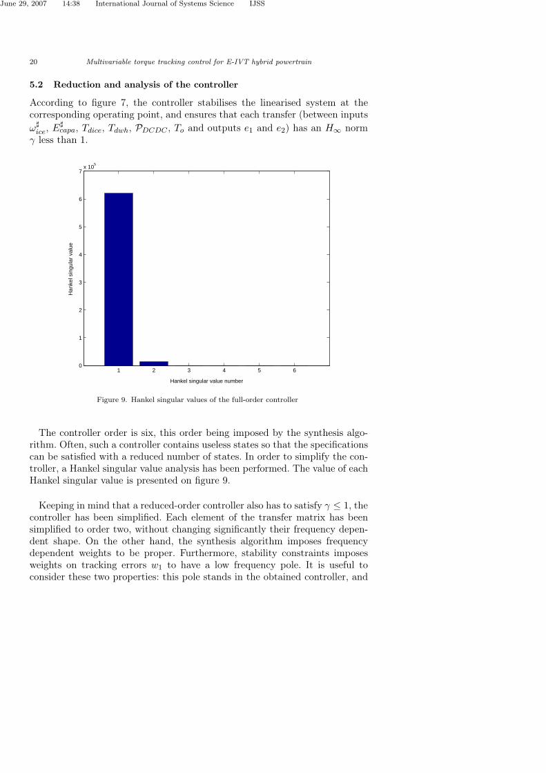
June 29, 2007 14:38 International Journal of Systems Science IJSS
20 Multivariable torque tracking control for E-IVT hybrid powertrain
5.2 Reduction and analysis of the controller
According to figure 7, the controller stabilises the linearised system at thecorresponding operating point, and ensures that each transfer (between inputsω]
ice, E]capa, Tdice, Tdwh, PDCDC , To and outputs e1 and e2) has an H∞ norm
γ less than 1.
1 2 3 4 5 60
1
2
3
4
5
6
7x 10
5
Hankel singular value number
Han
kel s
ingu
lar
valu
e
Figure 9. Hankel singular values of the full-order controller
The controller order is six, this order being imposed by the synthesis algo-rithm. Often, such a controller contains useless states so that the specificationscan be satisfied with a reduced number of states. In order to simplify the con-troller, a Hankel singular value analysis has been performed. The value of eachHankel singular value is presented on figure 9.
Keeping in mind that a reduced-order controller also has to satisfy γ ≤ 1, thecontroller has been simplified. Each element of the transfer matrix has beensimplified to order two, without changing significantly their frequency depen-dent shape. On the other hand, the synthesis algorithm imposes frequencydependent weights to be proper. Furthermore, stability constraints imposesweights on tracking errors w1 to have a low frequency pole. It is useful toconsider these two properties: this pole stands in the obtained controller, and

June 29, 2007 14:38 International Journal of Systems Science IJSS
O. REYSS, G. DUC, P. POGNANT-GROS and G. SANDOU 21
Figure 10. full-order (solid line) and simplified (dashed line) controllers Bode diagrams
the lowest the frequency of this pole is, the better the performances are. As aresult, it is gainful to substitute such poles by zero poles.
Such a simplified controller K1 is composed of 4 PI controllers, with highfrequency filtering. The order of the simplified controller is four. Figure 10presents full-order and simplified controllers Bode diagrams. As a result, wewill now call K1 the simplified controller (tracking ωice and Ecapa)).
5.3 Controller analysis
The model required to design the controller is different from the real system(that is non-linear). Considering the real system, ωe1 and ωe2 vary inside thepolytope AB of figure 8. Moreover, the whole system is now considered, that’sto say the closed-loop part (K1, tracking ωice and Ecapa, see figure 5) and theopen loop part (K2, tracking To). Every guarantees on stability and perfor-mances given by H∞ synthesis are lost. As a result, the use of stability andperformance analysis tools is necessary.

June 29, 2007 14:38 International Journal of Systems Science IJSS
22 Multivariable torque tracking control for E-IVT hybrid powertrain
Figure 11. µ upper and lower bounds (system in ωe1 = ωe1max2
rad.s−1 and ωe2 = ωe2minr
ad.s−1)
5.3.1 Linear analysis. First, slow variations of ωe1 and ωe2 are considered.If those variations are slow enough, it is possible to consider that they have noinfluence on stability and performances. Then, it is possible to see ωe1 and ωe2
as invariant uncertain parameters instead of varying parameters. The stabilityand the performances of the system is given by its analysis on each point of thepolytope. Considering this hypothesis, µ-analysis (see Zhou et al. (1996)) hasbeen performed and showed stability on the whole polytope. Considering themodel linearised for ωe1 = ωe1max
r ad.s−1 and ωe2 = ωe2min
r ad.s−1, and using realparameter uncertainties with unit norm, 0.002 is obtained as the maximumof µ upper bound (see figure 11). It shows that the system is stabilised forωe1 ∈ [0;ωe1max]rad.s−1 and ωe2 ∈ [ωe2min; 0]rad.s−1. Using such a method,it is therefore possible to shows that the system is stabilised on the wholepolytope.
Transfers between references and disturbances, and tracking errors and con-trol inputs are helpful tools to analyse performances of the system. Althoughperformances are worst on the corners, these stands convenient, and the spec-ifications are satisfied on the whole polytope.

June 29, 2007 14:38 International Journal of Systems Science IJSS
O. REYSS, G. DUC, P. POGNANT-GROS and G. SANDOU 23
5.3.2 Robust stability in the polytope. It is possible to write the statespace description of the system as follows:
xS = ASxS + BS(θ)uS
y = CSxS + DSuS
where xS is the state vector, uS is the control input vector and y is the outputvector, AS , CS and DS are constant matrices and BS is a matrix that linearlydepends on θ that is time varying in the polytope Θ.
A controller being designed, it is possible to write the state space descriptionof the closed-loop system, named SBF , as:
x = A(θ)x + B(θ)u
y = C(θ)x + D(θ)u
where x is the state vector, u is the input vector and y the output vector ofthe closed-loop system, A(θ), B(θ), C(θ) and D(θ) are matrices that linearlydepends on θ that is time varying in the polytope Θ. Indeed, these matricesare varying because they are dependent on BS .
One of the most common tools to study the stability of a LTI (linear timeinvariant) system is the quadratic Lyapunov stability.Lyapunov stability:An equilibrium point x0 is Lyapunov stable if it is possible to find a function
V (x) satisfying:
(i) V (x) > V (x0) for x 6= x0
(ii) ddt(V (x)) < 0 for x 6= x0
Such a function V (x) is called energy function of the system.
When V (x) = (x − x0)T P (x − x0) with P = P T > 0, quadratic stability issatisfied. Considering a linear time invariant system, A its state matrix andx = 0 as an equilibrium, this definition is equivalent to solving the followinglinear matrix inequalities (LMI), whose unknown is P :
P > 0 (8)

June 29, 2007 14:38 International Journal of Systems Science IJSS
24 Multivariable torque tracking control for E-IVT hybrid powertrain
AT P + PA < 0
Gahinet et al. (1994) and Gahinet et al. (1996) show it is possible to extendthis theory to polytopic LPV systems. It means that the varying system isalways a barycenter of the linearised systems on the corners of the polytope.Furthermore, if the system is a polytopic LPV system, so does the closed-loopsystem. As a result:
A(θ(t)) =∑
i αi(t)Ai with 0 ≤ αi(t) ≤ 1 and∑
αi(t) = 1
where Ai are the state matrices of the linearised system on each corner ofthe polytope.
Now, consider a constant matrix P being positive, such that quadratic Lya-punov stability is satisfied on each corner of the polytope (on linearised sys-tems), that is to say, such that:
ATi P + PAi < 0 for every i
Then, we have: αi(t)ATi P + Pαi(t)Ai < 0 for every i and every t∑
i αi(t)ATi P + P
∑i αi(t)Ai < 0 for every t
Thus A(t)T P + PA(t) < 0
This is an important result, because it shows that finding such a constant Pmatrix satisfying (8) on each corner of the polytope proves Lyapunov quadraticstability for every variation of the parameters on the whole polytope. Note thatthis is only a sufficient condition.
This analysis has been performed on the system and it has shown that thesystem is stable for every arbitrarily variations of ωe1 and ωe2 in the polytope.
6 Controllers, for two different specification sets
6.1 Examples of specifications
One of the main advantages of this method is the possibility to change speci-fications very sharply, by shaping frequency dependent weights. To show dif-ferences between two sets of specifications, based on paragraph 2.1.3, two con-trollers are considered.
First, a controller with hard constraints on ωice and To is designed. Specifi-cations are:

June 29, 2007 14:38 International Journal of Systems Science IJSS
O. REYSS, G. DUC, P. POGNANT-GROS and G. SANDOU 25
τωice τTomax(|U ref
capa − Ucapa|)100ms as fast as possible 25V
The aim of this synthesis is to get a controller able to track ωice during hardsimulation events.
Then, a controller with hard constraints on Ecapa is designed. Face to simu-lations close to a real driving cycle, specifications are:
τωice τTomax(|U ref
capa − Ucapa|)100ms as fast as possible 2V
6.2 Simulations
In order to check the performances of these controllers, a complete discretemodel of the vehicle is required, with:
(i) ICE and electric machines limitations,(ii) delays as on the real powertrain (measures...),(iii) system non-linearities (capacitor charge, depending on ωe1 and ωe2),(iv) disturbances (mostly Tdice, Tdwh, Pdcdc).
Because the system is non-linear, it is not possible to test each scenarii and toget exhaustive results. But simulations on the whole polytope give significantresults.
First specification setSeveral types of events happen during the simulation. It is possible to change
the value of: the ICE speed and the wheel torque references, the battery chargeor discharge power PDCDC , and consequently the electric machines and thevehicle speeds. Figure 12 shows ωice, To and Ucapa and their references. On thisfigure, we also draw Pdcnormalis, that is equal to P divided by its maximumand centered, in order to be easily compared to other variables. Studying theTe1, Te2 and Tice torques may also be interesting to verify that they remaininside the specifications (figure 13). Figure 14 presents ωe1 and ωe2, as well asVvh, in order to see where the system is on the polytope.
Second specification setHere, the same events are simulated. Results are presented on figures 15 and
16. Vehicle and electric machines speeds are the same as on figure 14.

June 29, 2007 14:38 International Journal of Systems Science IJSS
26 Multivariable torque tracking control for E-IVT hybrid powertrain
Figure 12. First specification set: ωice, To and Ucapa and references
The specifications are satisfied in both cases. The time response for ωice issmaller than 100ms, To is fast enough and Ucapa stands in an appropriate range.The controlled-outputs behaviors are well decoupled: for example, during awheel torque step, the ICE speed and the buffer-capacitor voltage variationsare not significant. Pdcdc and other disturbances are rejected.
Differences are shown between these two controllers. The second one ensuresa more precise tracking of Ucapa. To get such a behavior, constraints on ωice
and To has been decreased, but it is not visible on these figures. It is possibleto see such differences by performing harder simulations.
These simulations show that a LTI controller give convenient results. Forharder simulation events, or with a different polytope the design of a LPVcontroller may be needed.

June 29, 2007 14:38 International Journal of Systems Science IJSS
O. REYSS, G. DUC, P. POGNANT-GROS and G. SANDOU 27
Figure 13. First specification set: actuators torques
7 Conclusion
The hybrid electric vehicle described in this paper is a potential solution toreduce CO2 emissions and fuel consumption. Such hybrid transmissions arenon-linear multivariable systems: the three output variables (ICE speed, bat-tery charge and wheel torque) are fully dependent on the three actuators (oneICE and two electric machines). Furthermore, energetic control specificationinvolves non-linearity. This makes the control law be complex and hardly tun-able. In order to simplify this problem, a two-level control structure has beendefined in order to imitate a classic powertrain behavior. A controller has beendesigned using H∞ synthesis and led to a LTI controller on an operating point.This model-based design approach directly deals with robustness and decou-pling, in a full multivariable (2× 2) and frequency-dependent framework. ThisLTI controller has been analysed with a LPV analysis tool, in order to checkthe robustness of stability and performances. Finally, simulation of the closed-loop system have been performed, showing the design approach capabilities tosatisfy precise specifications. Since the results are very convincing, this controllaw will be implemented into a prototype.

June 29, 2007 14:38 International Journal of Systems Science IJSS
28 Multivariable torque tracking control for E-IVT hybrid powertrain
Figure 14. Vehicle and electric machines speeds
REFERENCES
A. Villeneuve, "Dual mode electric infinitely variable transmission", Aachenerkolloquium fahrzeug- und motorentechnik (2004).
D.J Leith, W.E Leithead, "Survey on gain-scheduling analysis and design",International journal of control (2000).
A. Helmersson, "Methods for robust gain scheduling", Phd Thesis, Linköpinguniversity (1995).
J.C. Doyle, K. Glover, P.P. Khargonekar, B. Francis, "State space solutions forH2 and H∞ control problems", IEEE transactions on automatic control(1989).
P. Gahinet, P. Apkarian, M. Chilali, "Affine parameter-dependent Lyapunovfunctions for real parametric uncertainty", Proceedings of the 33rd con-ference on decision and control (1994).
P. Gahinet, P. Apkarian, M. Chilali, "Affine parameter-dependent Lyapunovfunctions and real parametric uncertainty", IEEE transactions on auto-matic control (1996).
K. Glover, J.C. Doyle, "State space formulae for all stabilizing controllers thatsatisfy an H∞-norm bound and relations to risk sensitivity", Systems andcontrol letters (1988).
P. Apkarian, P. Gahinet, "A linear matrix inequality approach to H∞ control",

June 29, 2007 14:38 International Journal of Systems Science IJSS
O. REYSS, G. DUC, P. POGNANT-GROS and G. SANDOU 29
Figure 15. Second specification set : ωice, To and Ucapa and references
Int. of robust and non linear control (1994).K. Zhou, J.C. Doyle, K. Glover, Robust and optimal control, Prentice-hall
(1996).

June 29, 2007 14:38 International Journal of Systems Science IJSS
30 Multivariable torque tracking control for E-IVT hybrid powertrain
Figure 16. Second specification set: actuators torques

Ant Colony and Genetic Algorithm forConstrained Predictive Control of Power
Systems
Guillaume Sandou and Sorin Olaru
Supelec, Automatic Control Department3, rue Joliot Curie, F-91192 Gif-sur-Yvette, France
Guillaume.Sandou,[email protected]
Abstract. In this paper, a cooperative metaheuristic based on antcolony optimization and genetic algorithm is developed for constrainedpredictive control of power systems. The classical Unit Commitment so-lution is an open loop control for power systems which cannot be appliedto real system, since it is affected by important uncertainties, a typicalsource being the consumer load. Predictive control offers an efficient wayto use optimization results in a closed loop framework, implying the on-line solution of successive constrained mixed optimization problems. Thealgorithm proposed here is able to explicitly deal with constraints, andto quickly find high quality suboptimal solutions for computationallyinvolving predictive control schemes. Simulation results show the effi-ciency of the developed method, even for Unit Commitment problemswith underestimated consumer demand.
1 Introduction
The control of hybrid systems necessitates pertinent answers to several chal-lenging problems, like the switching between different operating regimes, theinteraction of continuous-time and discrete event subsystems and the overallsatisfaction of operational constraints [1]. An inherent question is whether theclassical automatic control methods (for example frequency domain shaping oroptimal control) can be adapted in a systematic manner to the design of controllaws for hybrid systems. It turns out that the answer is generally negative (dueto the structural disparity) with a notable exception, that of predictive controllaw [2]. Indeed this technique, which is based on finite time optimal controlproblems over a receding horizon, has the important advantage of being a time-domain design procedure and thus being effective in the hybrid systems frame-work, too.
Optimizing the evolution of the hybrid system over a receding horizon gener-ally leads to mixed integer quadratic/linear programs (MIQP/MILP) which arecomputationally involving (NP-complete problems) due to the presence of logi-cal optimisation arguments. The exact solvers have a worst case combinatorialcomplexity as it is the case for example with the classical branch and bound
A. Bemporad, A. Bicchi, and G. Buttazzo (Eds.): HSCC 2007, LNCS 4416, pp. 501–514, 2007.c© Springer-Verlag Berlin Heidelberg 2007

502 G. Sandou and S. Olaru
routines, even if they are tailored to the problem specificity [3]. The real-timeimplementation constraints might force the optimization routines to act on a rel-ative short time interval and to offer at least a feasible suboptimal solution. Thiscan be obtained in a slightly different manner by renouncing to the exhaustivesearch and the use of evolutionary methods.
Figure 1 presents a classification for the MPC implementations. In a firststage, a cautious control design would pass by the tuning of the prediction hori-zon such that the attainability demands to be met and the optimization problemto be simplified. However, the real-time implementation would be resumed by aMIQP/MILP or MINP if nonlinearities are considered.
Fig. 1. A classification of predictive control possible implementations

Ant Colony and Genetic Algorithm 503
The same figure presents a demarcation between the implementations basedon on-line optimisation and those where an explicit analytical dependence of theoptimum on the current state is available [4]. In the second case, there is no needfor on-line optimisation, the computational load being reduced to the evaluationof the analytical function which gives the exact solution. Unfortunately explicitsolution can be practically constructed only for control problems with few statesand small prediction horizon due to the curse of dimensionality.
Returning to the classification, on the on-line implementation part a separa-tion can be made between the exact methods and the routines which allow fromthe design stage a certain degree of suboptimality as it is the case for examplewith genetic algorithms [5] or the Lagrangian relaxation where the quality of thesolution is improved, but it can not go beyond the duality gap.
In the present paper the attention will be given to cooperative metaheuristicsbased on ant colony optimization and genetic algorithm situated on the class ofsuboptimal methods. From the standpoint of computational complexity, findingout if an MIQP model has a feasible solution is essentially as hard as actuallyfinding the optimum. Branch and Bound procedures, for example, have to explorethe entire search tree to prove this. The developed algorithm proves to havethe ability of proposing (high quality) feasible solutions due to the contraintshandling mechanism.
For the sake of illustration, a popular problem in power systems will be used,the Unit Commitment. Indeed, power systems can be casted in the class ofhybrid systems since they have to be controlled both by integer variables (on/offvariables) and real variables (produced powers when switched on). Benefitingfrom this practical aspects, the details of the algorithm will be described in apractical manner.
The paper is organized as follows. The predictive control of power systems ispresented in section 2. This control law is based on a scheduling algorithm. Thisscheduling algorithm has to be highly tractable even for such large scale mixed in-teger optimization problems. Furthermore it has to take into account all technicalconstraints of the system. That is why a cooperative stochastic method using antcolony optimization and genetic algorithm has been developed and is depicted insection 3. Numerical results are given in section 4, showing the efficiency of theproposed control method even in the case of underestimated consumer demand.Finally, conclusions and forthcoming works are drawn in section 5.
2 Predictive Control of Power Systems
2.1 Open Loop Control and Unit Commitment
Unit Commitment is a classical large scale mixed integer problem in power sys-tems, which aims to compute the optimal scheduling of several production unitswhile satisfying consumer demand and technical constraints:
minuk
n,Qkn
m+N−1∑
n=m
(K∑
k=1
(ckprod(Q
kn, uk
n) + ckon/off(uk
n, ukn−1)
)). (1)

504 G. Sandou and S. Olaru
N is the length of time horizon, K the number of production unit, ukn (resp.
Qkn) the on/off status (resp. produced power) of production unit k during time
interval n. Production costs and start up and shut down costs are defined by:
ckprod(Q
kn, uk
n) = αk1Qk
n + αk0uk
n
ckon/off(uk
n, ukn−1) = ck
onukn(1 − uk
n−1) + ckoffuk
n−1(1 − ukn) . (2)
Integer variables are on/off status of production units, and real variables areproduced powers. The usual restriction comes from:
– capacity constraints
Qkminu
kn ≤ Qk
n ≤ Qkmaxu
kn, ∀n ∈ m, . . . , m + N − 1 , ∀k ∈ 1, . . . , K , (3)
– consumer demand satisfaction
K∑
k=1
Qkn ≥ Qdem
n , ∀n ∈ m, . . . , m + N − 1 , (4)
– time up and time down constraints⎧⎨
⎩
(uk
n−1 = 0, ukn = 1
)⇒
(uk
n+1 = 1, ukn+2 = 1, · · · , uk
n+T kup−1 = 1
)
(uk
n−1 = 1, ukn = 0
)⇒
(uk
n+1 = 0, ukn+2 = 0, · · · , uk
n+T kdown−1 = 0
) , (5)
– ramp constraints∣∣Qk
n − Qkn−1
∣∣ ≤ ΔQk, ∀n ∈ m, . . . , m + N − 1 , ∀k ∈ 1, . . . , K . (6)
Discrete dynamics on the system are expressed through logical equations (5) andcontinuous dynamics are stated as power increment limitations (6).
2.2 Closed Loop Control
For optimisation, consumer demand is supposed to be perfectly known over thewhole time horizon: the computation of the optimal scheduling is a referencetrajectory for integer and real control inputs. However, prediction errors of theconsumer load may lead to a deficient behavior. Thus, a closed loop control isrequired: the problem refers to the control of a hybrid system. A convenient wayto extend optimisation results in a closed loop framework is the receding horizon.The closed loop structure is presented in figure 2.
The idea is to compute the optimal scheduling on time interval [m, m+N −1],considering predicted consumer load Qdem
n . The first values of integer schedulingare applied to the system. Simultaneously, real variables are slightly updated soas to fulfill, if possible, the real demand at time m, Qdem
m . Production unit localregulations are assumed to be perfect: if production unit k has produced Qk
m−1during time interval m − 1, it can produce, if still switched on, whatever powerin the range [max(Qk
m−1 − ΔQk, Qkmin), min(Qk
m−1 + ΔQk, Qkmax] during time
interval m. The scheduling algorithm will now be detailed.

Ant Colony and Genetic Algorithm 505
Fig. 2. Closed loop control synopsis
3 Optimization Procedure
3.1 Optimization Methods Analysis and Proposition of a WellSuited Algorithm
Numerous methods have been applied to solve Unit Commitment and relatedproblems such as facility location. They are listed for instance in [6] and are herebriefly depicted. Exact solution methods (exhaustive enumeration, Branch andBound [7], dynamic programming [8]) have been tested. These methods sufferfrom combinatorial complexity: an efficient approximated method is requested.Deterministic approximated methods can be used (priority lists in [9]). But, dueto numerous constraints, they are often strongly suboptimal. Constraints areexplicitly considered using Lagrangian relaxation [10]. Coupling constraints arerelaxed, and the problem is divided into several optimisation problems (one perproduction unit). However, no guarantee can be given on the actual optimality.Further, an iterative procedure has to be performed: solution of the optimisa-tion problems and updating of Lagrange multipliers. The update can be madewith genetic algorithms [11] or subgradient methods [12]. For large scale cases,metaheuristics are interesting methods: simulated annealing in [13], tabu searchin [14] and genetic algorithms in [15]. No guarantee can be given on the actualoptimality of the solution, but an often suitable solution with low computationtimes can be found. One of the problems of these methods is the handling ofconstraints. The algorithm ”moves” randomly in the search space, and so, there is

506 G. Sandou and S. Olaru
no guarantee that the final solution is in the feasible set. This is particularly thecase for Unit Commitment, as the feasible set is much smaller than the searchspace.
Considering these arguments, ant colony appears to be an efficient way tosolve this kind of problems, as it is able to find near optimal solutions with anexplicit handling of all constraints. Indeed, ant colony is a constructive stochasticalgorithm and solutions are explicitly built as feasible ones (see section 3.2). Fromthis initial population of ”medium quality solutions” quickly computed by antcolony, a feasibility criterion is defined (see section 3.4). Genetic algorithm is thenused to intensively explore the search space (see section 3.5), with an implicitmanagement of problem constraints. Indeed, due to a positive feedback in the antcolony algorithm formulation, it may converge to a local minimum. An intensiveexploration of the search space is thus required to circumvent this issue, andgenetic algorithm, which is an efficient stochastic algorithm for unconstrainedproblems is used. Note that the algorithm supposes that real variables are quicklycomputed: the developed cooperative algorithm is also hybridized with an exactsolution algorithm for real variables (see section 3.3). Finally, this method allowssimultaneously using the interesting properties of ant colony (explicitly handlingof constraints) and of genetic algorithm (deep exploration of the search space,and so high quality of the solution). The general synopsis of the method isdepicted on figure 3.
Fig. 3. Cooperative algorithm synopsis
3.2 Ant Colony Optimization
Real world ants. Ant colony optimization was firstly introduced by MarcoDorigo [16] and [17]. It is based on the way ants are looking for food.
Suppose (see figure 4a), that ants have managed to find food. Each particu-lar ant does not know where to go. It only chooses its path depending on thepheromone trail which has been laid on the ground by previous ants. If the pathof pheromone is broken because of an obstacle, see figure 4b, first ants randomly
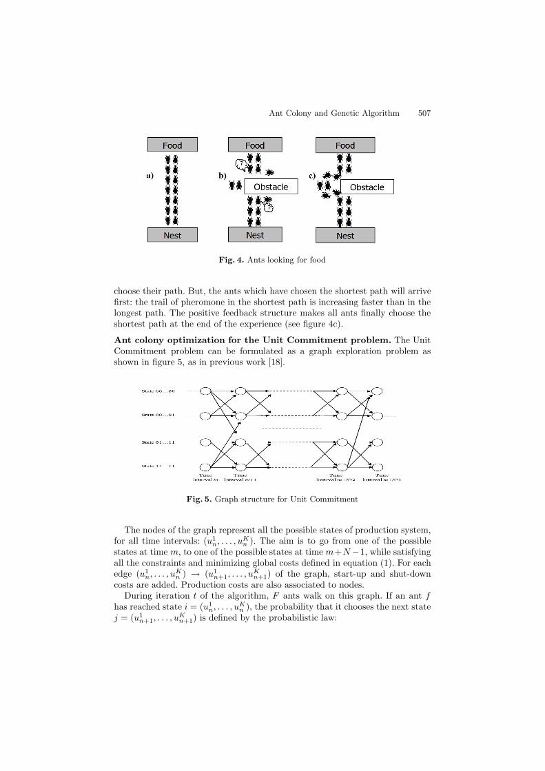
Ant Colony and Genetic Algorithm 507
Fig. 4. Ants looking for food
choose their path. But, the ants which have chosen the shortest path will arrivefirst: the trail of pheromone in the shortest path is increasing faster than in thelongest path. The positive feedback structure makes all ants finally choose theshortest path at the end of the experience (see figure 4c).
Ant colony optimization for the Unit Commitment problem. The UnitCommitment problem can be formulated as a graph exploration problem asshown in figure 5, as in previous work [18].
Fig. 5. Graph structure for Unit Commitment
The nodes of the graph represent all the possible states of production system,for all time intervals: (u1
n, . . . , uKn ). The aim is to go from one of the possible
states at time m, to one of the possible states at time m+N −1, while satisfyingall the constraints and minimizing global costs defined in equation (1). For eachedge (u1
n, . . . , uKn ) → (u1
n+1, . . . , uKn+1) of the graph, start-up and shut-down
costs are added. Production costs are also associated to nodes.During iteration t of the algorithm, F ants walk on this graph. If an ant f
has reached state i = (u1n, . . . , uK
n ), the probability that it chooses the next statej = (u1
n+1, . . . , uKn+1) is defined by the probabilistic law:

508 G. Sandou and S. Olaru
p(f)i (j) =
ηαijτij(t)β
∑m∈Jf (i)
ηαimτim(t)β
. (7)
– τij(t) is the pheromone trail on edge i=(u1n, . . . , uK
n ) → j = (u1n+1, . . . , u
Kn+1)
during iteration t. Its value depends on the results of previous ants.– ηij is the attractiveness. It refers to the ” local choice ”. When next node has
to be chosen, the best local candidate is the node for which the gap betweenthe maximum produced power and the predicted demand is the smallest. Itis not sure that this is the best ”global” choice, as the security margin isquite low. For more details, see previous work [18].
– α and β are weighting factors.– Jf (i) is the feasible set. This feasible set contains a priori all 2K states. But,
those states which do not satisfy time up and time down constraints, andthose states which do not satisfy consumers’ demands, are to be removed.Note that, even if produced powers are not known yet, it is possible to checkthe possibility of consumer’s demand satisfaction with the equation:
K∑
k=1
((Qk
min(1 − ukn)+(
min(Qkmax, Q
kn + ΔQk)
)uk
n
)uk
n+1
)≥ Qdem
n+1. (8)
Jf (i) sets are recursively constructed for each ant, and lead to the guarantee ofthe feasibility of solutions. After the ant has completed its path, it is possible toevaluate the solution by solving the real optimisation problem defined in equation(1), with fixed binary variables. Due to the positive feedback of the algorithmthe past mistakes have to be forgotten to avoid premature convergence. This isdone by the pheromone evaporation. The pheromone trail is updated:
τij(t + 1) = (1 − ρ)τij(t) + Δτij(t) (9)
ρ is the evaporation coefficient. This coefficient is viewed as an analogy withnatural evaporation. Δτij is the updating coefficient, depending on the resultsof ants in iteration t. An elitism algorithm is used: only the best ant is allowedto lay some pheromone on each edge it has used. The ant evaluation supposesthe computation of real variables, which will now be depicted.
3.3 Computation of Real Variables
Binary variables are computed by ant colony. For each feasible sequence ukn the
corresponding real variables Qkn are computed as the solution of:
arg minQk
n
m+N−1∑n=m
(K∑
k=1
(ckprod
(Qk
n, ukn
)+ ck
on/off
(uk
n, ukn−1
)))
= arg minQk
n
(m+N−1∑
n=m
K∑k=1
(ckprod
(Qk
n, ukn
)))
= arg minQk
n
(m+N−1∑
n=m
K∑k=1
αk1Qk
nukn + αk
0ukn
)= arg min
Qkn
(m+N−1∑
n=m
K∑k=1
αk1Qk
nukn
)
(10)

Ant Colony and Genetic Algorithm 509
As there are no temporally coupling constraints anymore (they have been guar-anteed by the constructive ant colony algorithm), the problem can be dividedinto N successive optimisation problems:
minQk
n,k=1,...,K
(K∑
k=1αk
1Qknuk
n
)
subject to
⎧⎪⎪⎪⎪⎪⎨
⎪⎪⎪⎪⎪⎩
K∑k=1
Qkn ≥ Qdem
n
Qkminu
kn ≤ Qk
n ≤(
Qkmin(1 − uk
n−1)+(min(Qk
max, Qkn−1 + ΔQk)
)uk
n−1
)
︸ ︷︷ ︸=Qk
max(n)
ukn
(11)
Without loss of generality, consider that α11 ≤ α2
1 ≤ . . . ≤ αK1 . Then, the
optimal solution of problem (10) is to produce as much as possible with low-cost units, while satisfying capacity constraints. Then, the following recursivealgorithm is performed:
⎧⎪⎪⎪⎪⎪⎪⎪⎪⎪⎪⎪⎪⎪⎨
⎪⎪⎪⎪⎪⎪⎪⎪⎪⎪⎪⎪⎪⎩
Q1n = min
(max
(Qdem
n −K∑
i=2Qi
minuin, Q1
min
), Q1
max(n))
u1n
...
Qkn = min
(max
(Qdem
n −k−1∑i=1
Qin −
K∑i=k+1
Qiminu
in, Qk
min
), Qk
max(n)
)uk
n
...
QKn = min
(max
(Qdem
n −K−1∑i=1
Qin, QK
min
), QK
max(n))
uKn
Qkmax(n + 1) = Qk
min(1 − ukn) +
(min(Qk
max, Qkn + ΔQk)
)uk
n
(12)
3.4 Feasibility Criterion
To compute a feasibility criterion one has just to know a feasible solution. If thecost of this feasible known solution is cf , the feasibility criterion can be:
minuk
n, Qkn
n = 1, · · · , Nk = 1, . . . , K
⎛
⎝N∑
n=1
K∑k=1
(ckprod
(Qk
n, ukn
)+ ck
on/off
(uk
n, ukn−1
))
+((1 + ε) cf + h
(uk
n, Qkn
))B
(uk
n, Qkn
)
⎞
⎠ (13)
where one can distinguish:
– ε is a small positive real,– h
(uk
n, Qkn
)is a penalty function for non feasible solutions
uk
n, Qkn
,
– B(
ukn, Qk
n
)is a boolean function with value 1 for non feasible solutions
and 0 for feasible ones.

510 G. Sandou and S. Olaru
With this criterion, all infeasible solutions will have a higher cost than the costof the feasible known solution. For feasible solutions, the penalty is null, and theinitial cost function is just considered. Finally, any unconstrained optimisationalgorithm can be used to solve the problem, the constraints being implicitlytaken into account. In this study, the known feasible solution is the best solutionfound by ant colony optimization.
3.5 Knowledge Based Genetic Algorithm
Classical genetic algorithm. A knowledge based genetic algorithm, similarto the one developed in current work [19] is used. The general flow chart of agenetic algorithm is called up in figure 6.
Fig. 6. Flow chart of a genetic algorithm
The main idea is to make a population of potential solutions evolves to createnew solutions by using stochastic (or ”genetic”) operators. In this cooperativemethod, the initial population is made of all feasible solutions computed by antcolony optimization. Classical operators are crossing-over operator and mutationoperator (see figure 7). For the crossing over operation, two potential solutionsare randomly chosen in the population. They randomly merge their variables(or ”genes”) to create two new solutions. The mutation operation is the randomselection of a potential solution and of one of its genes. This gene is changed toanother. The aim of this operator is to keep the population genetic diversity.
The selection operator is an operator which aims to choose a new popula-tion from parents and children. This operation is made using the roulette wheelselection. After having computed the fitness value of each individual in the pop-ulation, the probability of selection is proportional to the quality of individuals.Knowledge based operator. Classical genetic operators may not be wellsuited to Unit Commitment problem. Consider for instance the situation of fig-ure 8. Because of time down and time up constraints, a random mutation willvery often lead to an infeasible solution. Switching times are particular points of

Ant Colony and Genetic Algorithm 511
Fig. 7. Classical crossing-over (a) and mutation (b) operators
Fig. 8. Selective mutation operator
the solution where a mutation has a higher probability to create a new feasiblesolution. Thus, a selective mutation operator has been designed. Switching timesare detected, and mutations are allowed only for these genes. No guarantee onthe feasibility is achieved, but the ”probability of feasibility” is higher.
4 Simulation Results
4.1 Real Time Updating of Produced Powers
As already explained, the ”optimal” scheduling of the power system is computedfrom predicted values Qdem
n on time interval [m, m + N − 1]. The first valuesof integer scheduling uk
m are applied to the system. Real variables are updated

512 G. Sandou and S. Olaru
Table 1. Characteristics of the benchmark example
Unit Qmin Qmax ΔQ α0 α1 con coff Tdown Tup
(MW) (MW) (MW) (AC) (AC/MWh) (AC) (AC) (h) (h)1 10 40 10 25 2.6 10 2 2 42 10 40 10 25 7.9 10 2 2 43 10 40 10 25 13.1 10 2 3 44 10 40 10 25 18.3 10 2 3 4
Fig. 9. Simulation results
at time m, when real value Qdemm is known, using the equation (12) considering
Qdemm instead of Qdem
n . These values are given to the scheduling procedure attime m+1, for instance for the satisfaction of ramp constraints.
4.2 Case Study
To test the algorithm, a ”four unit” academic case is considered. The charac-teristics of this case are given in table 1. A worst case is considered: consumerload is always underestimated. The prediction error is a random value in therange [−5%, 0%]. The time horizon is N = 24 hours. Consumer load has a dailyoscillation. Thus, the dynamic of the system is about 24 hours and the timehorizon has to be greater: a high value has to be given to N . The simulation isperformed on a 4 day total horizon. Results, obtained with Matlab 6.5 on a PIV2GHz, are given on figure 9.
Results show that the production is very close to the real demand, exceptfor some peaks which have been underestimated. The optimization of the 96binary variable problem is performed in just 25 seconds with the developed antcolony/genetic algorithm method. Due to the computation of successive econom-ical near optimal solutions and real time slight updates, global costs are veryclose to global optimal costs. More precisely, a comparison has been performedwith classical MILP solver, with a ”Branch and Bound” method. It shows thatthe developed metaheuristic optimisation algorithm can compute a sub-optimal

Ant Colony and Genetic Algorithm 513
solution with a mean slight increase of 0.4% compared with the optimal solution.Furthermore, the MILP solver is very sensitive to the problem characteristicssuch as start up and shut down costs, leading to varying computation timesgoing from 10 seconds to 10 hours. Finally, the algorithm has been tested for10-unit case, leading to satisfying results with 10 minute computation times, andfor which MILP solver is untractable.
5 Conclusions and Perspectives
In this paper a control structure has been defined for power systems. A meta-heuristic algorithm, based on ant colony and genetic algorithm, is used to per-form the solution of Unit Commitment. As this kind of algorithm is highlytractable and explicitly manage all the constraints of the problem, it can beused to extend the optimization results in a closed loop real time framework.
This study is an experimentation of the use of stochastic algorithms for pre-dictive control of hybrid systems. Of course, the main drawback of the proposedmethod is that no guarantee can be given on the actual optimality of solutions.Further, the problem of stability of the closed loop predictive control structureis a very tough task. However, the use of ant colony for the constrained predic-tive control of hybrid systems is promising. The proposed algorithm is tractableeven for large scale systems and could be applied to various kinds of systemssuch as non linear or non analytical systems. Further, numerous constraints canbe explicitly taken into account as the proposed method is based on a construc-tive algorithm. Finally, it allows the use of large receding horizons. Forthcomingworks deal with the use of such algorithms in a more general framework forcontrol of generic non linear constrained hybrid systems.
References
1. Branicky M.S., Borkar V.S., Mitter S.K.: A unified framework for hybrid control:model and optimal control theory, IEEE Transaction on Automatic Control, 43,(1998), 31-45.
2. Mayne D.Q., Rawlings J.B., Rao C.V., Scockaert P.O.M.: Constrained model pre-dictive control: Stability and optimality, Automatica, 36, (2000),789–814.
3. Fletcher R., Leyffer S., ”Numerical experience with lower bounds for MIQP branchand bound”, Technical report, Dept. of Mathematics, University of Dundee, Scot-land. http://www.mcs.-dundee.ac.uk:8080/sleyffer/miqp art.ps.z, (1995).
4. Bemporad A., Borelli F., Morari M.: Piecewise Linear Optimal Controllers forHybrid Systems, IEEE American Control Conference, (2000).
5. Olaru S., Thomas J., Dumur D., Buisson J.: Genetic Algorithm based Model Pre-dictive Control for Hybrid Systems under a Modified MLD Form, InternationalJournal of Hybrid Systems, 4, (2004), 113-132.
6. Sen S., Kothari D. P.: Optimal Thermal Generating Unit Commitment: a Review.Electrical Power and Energy Systems, 20(7), (1998), 443-451.
7. Chen C.-L, Wang S.-C.: Branch and Bound scheduling for thermal generating units.IEEE Transactions on Energy Conversion, 8, (1993), 184-189.

514 G. Sandou and S. Olaru
8. Ouyang Z., Shahidehpour S. M.: An intelligent dynamic programming for unitcommitment application. IEEE Transactions on Power Systems, 6, (1991), 1203-1209.
9. Senjyu T., Shimabukuro, K., Uezato K., Funabashi T.: A fast technique for UnitCommitment problem by extended priority list. IEEE Transactions on Power Sys-tems, 19, (2004), 2119-2120.
10. Zhai Q; Guan X.: Unit Commitment with identical units: successive subproblemssolving method based on Lagrangian relaxation. IEEE Transactions on Power Sys-tems, 17, (2002), 1250-1257.
11. Cheng C.-P., Liu C.-W., Liu C.-C.: Unit Commitment by Lagrangian Relax-ation and Genetic Algorithms. IEEE Transactions on Power Systems, 15, (2000),707-714.
12. Dotzauer E., Holmstrm K., Ravn H. F.: Optimal Unit Commitment and EconomicDispatch of Cogeneration Systems with a Storage. 13th Power Systems Computa-tion Conference, Trondheim, Norway (1999), 738-744.
13. Yin Wa Wong S.: An Enhanced Simulated Annealing Approach to Unit Commit-ment. Electrical Power & Energy Systems, 20, (1998), 359-368.
14. Rajan C. C. A, Mohan M. R.: An evolutionary programming-based tabu searchmethod for solving the unit commitment problem. IEEE Transactions on PowerSystems, 19, (2004), 577-585.
15. Swarup K . S., Yamashiro: Unit commitment solution methodology using geneticalgorithm. IEEE Transactions on Power Systems, 17, (2002), 87-91.
16. Dorigo M., Maniezzo V., Colorni A.: The Ant System: Optimization by a Colonyof Cooperating Agents. IEEE Transactions on Systems, Man and Cybernetics-PartB, 26, (1996), 1-13.
17. Dorigo M., Gambardella, L. M., Ant Colony System : a Cooperative LearningApproach to the Traveling Salesman Problem, IEEE Transactions on EvolutionaryComputation, 1 (1997), 53-66.
18. Sandou G., Font S., Tebbani S., Hiret A., Mondon C.: Optimisation par colonies defourmis d’un site de generation d’energie. Journal Europeen des Systemes Automa-tises, Numero special: Metaheuristiques pour l’optimisation difficile, 38, (2004),1097-1119.
19. Sandou G., Font S., Tebbani S., Hiret A., Mondon C.: Enhanced genetic algorithmwith gurantee of feasibility for the Unit Commitment problem, submitted to IEEETransactions on Power Systems.

Particle Swarm Optimization for the design of H static output feedbacks
Mohamed Yagoubi*, Guillaume Sandou**
*IRCCyN (Communications and Cybernetic Research Institute of Nantes) 1, rue de la Noë, 44321 Nantes, France
*EMN (Ecole des Mines de Nantes) 4, rue Alfred Kastler, 44307 Nantes, FRANCE
(Tel.: +33 2 51 85 83 27; e-mail: [email protected]) **SUPELEC Systems Sciences (E3S), Automatic Control Department
3, rue Joliot Curie, 91192 Gif-sur-Yvette, FRANCE (Tel: +33 1 69 85 13 86; e-mail: [email protected])
Abstract: The design of H reduced order controllers is known to be a non convex optimization problem for which no generic solution exists. In this paper, the use of Particle Swarm Optimization (PSO) for the computation of H static output feedbacks is investigated. Two approaches are tested. In a first part, a probabilistic-type PSO algorithm is defined for the computation of discrete sets of stabilizing static output feedback controllers. This method relies on a technique for random sample generation in a given domain. It is therefore used for computing a suboptimal H static output feedback solution. In a second part, the initial optimization problem is solved by PSO, the decision variables being the feedback gains. Results are compared with standard reduced order problem solvers using the COMPleib benchmark examples and appear to be much than satisfactory, proving the great potential of PSO techniques.
Keywords: Reduced order controllers, Particle Swarm Optimization, static output feedback, H synthesis
1. INTRODUCTION
H synthesis is an efficient tool in automatic control to compute controllers in a closed-loop framework, achieving high and various performances (Gahinet and Apkarian, 1994, Zhou, et al., 1996). The main drawback of such approaches is the controller order: H synthesis provides a controller whose order is the same as the synthesis model. A classical way to derive low order controllers is to use a full-order synthesis and to reduce the obtained controller. However, this kind of approach may lead to a high H norm of the closed-loop system and a high sensitivity to high frequency noises.
Another approach is to solve an H optimization problem, adding some order constraints on the solution. However, this kind of constraints is expressed by matrices rank constraints. Thus, the reduced-order synthesis problem appears to be a non-convex, non-smooth optimization problem. Several approaches exist, trying to overcome this difficulty:
Convex approximations of non-convex stability regions, but often obtained from conservative conditions;
Global nonlinear optimization techniques such as an exhaustive search, which are very expensive;
Local optimization techniques such as BMI solvers. In that case, the solution strongly depends on the initial controller.
More recently, some new techniques have began to emerge, adding some random process in the deterministic search algorithm (Arzelier, et al., 2010), and achieving results which are almost similar to those obtained with the HIFOO standard
(Burke, et al., 2006). Following this new trend, a new approach is proposed in this paper, based on Particle Swarm Optimization (PSO) to solve the H static output feedback synthesis problem. PSO was firstly introduced by Eberhart and Kennedy (Eberhart and Kennedy, 1995). This optimization method belongs to the class of approximated stochastic method called metaheuristics methods. With such methods, the optimality of the computed solution can never be guaranteed, but there are strong advantages:
The structure of costs and constraints is not an essential point as no gradient has to be computed;
The random part allows escaping from local minima.
Two approaches based on PSO are presented in the sequel. In the first one, a probabilistic-type PSO algorithm, to deal with the problem of building sets of stabilizing static output feedback controllers, is proposed. A suboptimal H static output feedback solution is then computed obviously by selecting the element achieving the best H performance in the constructed set. In this approach, the PSO algorithm is proposed to maximize an empirical estimate of the existence probability of static output feedback controllers in some bounded balls moving in the search space. The probability estimate is evaluated based on a random sample generation technique borrowed from (Calafiore, et al., 1999, Calafiore, et al., 2006). This technique produces a finite number of real random matrices uniformly distributed in a given domain.
The second approach deals with the direct optimization of output feedback gains, the optimization variables being the feedback gains.

The paper is organized as follows. The PSO algorithm is presented in section 2. For MIMO systems, a static output feedback may lead to numerous optimization variables and so a perturbed PSO algorithm is also presented. In section 3, a probabilistic-type PSO-based approach leading to discrete sets of stabilizing static output feedback controllers is presented. A direct H optimization of feedback gains is fully described in section 4. In the same section, an indirect application of PSO, based on the method described in section 3, is also proposed for solving the optimal H static output feedback problem. Comparisons with standard algorithms show much than satisfactory results which can be achieved with low computation loads. Finally conclusions and forthcoming works are drawn in section 5.
2. PARTICLE SWARM OPTIMIZATION
2.1 Classical algorithm
PSO was firstly introduced by Eberhart and Kennedy (Eberhart and Kennedy, 1995). This optimization method is inspired by the social behavior of bird flocking or fish schooling. Consider the following optimization problem:
min ( )x
f xcÎ
(1)
P particles are moving in the search spacec . Each of them
has its own velocity, and is able to remember where it has found its best performance. Each particle has also some “friends”. The following notations will be used:
k
px : position of particle p at iteration k ;
k
pv : velocity of particle p at iteration k ;
1 ,
arg min( ( ))k kp p
k
px b x
b f x-Î
= : best position found by particle p
until iteration k ;
( ) 1, 2, , k
pV x PÌ set of “friend particles” of particle
p at iteration k ;
, ( )
arg min ( )k ki p
k
px b i V x
g f xÎ Î
= best position found by the friend
particles of particle p until iteration k. The particles move in the search space c according to the
following transition rule:
1
0 1 21 1
. ( ) ( )k k k k k kp p p p p pk k k
p p p
v c v c b x c g x
x x v
+
+ +
= + Ä - + Ä -
= + (2)
In this equation:
Ä is the element wise multiplication of vectors;
0c is the inertia factor ;
1c (resp.
2c ) is a random number in the range
1[0, ]c
(resp. 2
[0, ]c ).
2.2 Perturbed PSO algorithm
The choice of parameters is very important to ensure the satisfying convergence of the algorithm. Lots of work have been done on the topic; see for instance (Shi and Eberhart, 1998; Trelea 2003). However the PSO algorithm may suffer from premature convergence to local minima, especially for optimization problems with numerous variables. This can be the case for static output feedbacks, as a MIMO plant with r measured outputs and m control inputs leads to r m´ optimization variables. To overcome this difficulty, some perturbed versions have been defined. The idea is to add a random movement to the best particle to avoid that behaviour. Following the algorithm given in (van den Bergh and Engelbrecht, 2002), the transition rule (2) for the best particle is reformulated into:
1
0 [0,1]
1 1
. ( ) (1 2 )k k k k k
p p p p
k k k
p p p
v c v g x r
x x v
r+
+ +
= + - + -
= +, (3)
where [0,1]r is a random vector in the range [0,1]. The value
of kr is updated after each time step by:
1
2 if _
0.5 if _
otherwise
k
ck k
ck
nb success s
nb failure f
r
r r
r
+
ìï >ïïïï= >íïïïïïî
(4)
where _nb success is the number of consecutive successes
and _nb failure the number of consecutive failures (a step
is a success if the best value found by the particles is
enhanced, and a failure otherwise). cs and
cf are 2 tuning
parameters. For more details, see for instance (Van den Bergh and Engelbrecht, 2002; Xinchao, 2010) and references therein.
3. PROBABILISTIC-TYPE PSO FOR STATIC OUTPUT FEEDBACK STABILIZATION
Some attempts to use PSO for the design of automatic control laws have already been presented for instance in (Sandou, 2009). The originality, however, of the method proposed in this paper is twofold:
It allows building discrete sets of stabilizing static output feedbacks: the use of random sample generation technique makes it possible to better scrutinize the set of stabilizing static output feedbacks which may be nonconvex and consisting of many disjoint domains.
It takes advantage of probabilistic information (probability estimate of the existence of a static output feedback in a predefined domain) which is not the case of a standard PSO method.
3.1 Problem statement
Consider the state space representation of the plant S :

1
1 11 12
21
( ) ( ) ( ) ( )
: ( ) ( ) ( ) ( )
( ) ( ) ( )
x t x t w t u t
z t x t w t u t
y t x t w t
ìï = + +ïïïS = + +íïï = +ïïî
A B B
C D D
C D
, (5)
where nx Î is the state vector, mu Î is the control
vector, ry Î is the measured outputs vector, 2mw Î is the input vector (reference and disturbance inputs), and
2rz Î is the controlled vector. All matrices are assumed to be of appropriate dimensions. The model (5) is assumed to be stabilizable by static output feedback, that is to say that there exists a control law ( ) ( )u t y t= K such that the closed-loop
of figure 1 is stable.
Fig. 1: Computation of static output feedbacks
The set of stabilizing static output feedback matrices is:
/ ( )m r -G = Î L + ÎK A BKC (6)
where ( )ML denotes the spectrum (all eigenvalues) of the
matrix M . The first problem tackled with in this paper is to
build a non trivial subset ns
G Ì G of 1ns ³ instances.
3.2 Sample generation problem
We describe here the method used for generating real matrix
samples m rÎK bounded in the gl norm ball of radius d
given by:
( ) , / , 1,2,m r m r
g ggd d´ ´Q = Î £ = ¥K K (7)
The problem can be reduced to multiple random vector generation for which the technique borrowed from (Calafiore, et al., 1999) can be used. It is an algorithm that returns a real
random vector mq Î uniformly distributed in ( ), m
gdQ .
The algorithm is based on a generalized gamma density
function ( ),a bG f , defined as:
( ) 1
,,
( )
bba f
a b
bG f f e f
G a- - += Î (8)
where a and b are given parameters and ( )G a is the
gamma function. We report here the algorithm used for this purpose in the Randomized Algorithms Control Toolbox (RATC) (http://ract.sourceforge.net).
Algorithm 1: (Uniform generation in a real gl norm ball)
Generate m independent real random scalars
1/ ,i g gGx Î ;
Construct the vector md Î of components i i id s ,
where is are independent random signs;
Generate 1/mh j= , where j is uniform in 0,1é ùê úë û ;
Return
g
dq h
dd= .
Remark 1: The solution for the case ( )2, m rd ´Q can also
be dealt with using RATC. A singular value decomposition is needed in that case. See (Tempo, et al. 2005) for more details.
3.3 Probabilistic-type PSO for static output feedback stabilization
The algorithm proposed in this section uses complementary advantages of:
The sample generation method described in section 3.2. The probabilistic information (which is often neglected
in a deterministic context) that consists in an empirical probability estimate of the existence of a static output feedback in some predetermined subsets.
The PSO (the meta-heuristic method described in section 2) property of escaping from local minima.
The main idea for building a set of stabilizing static output feedback controllers for the system given in (5) is summarized hereafter.
The following lines describe the proposed method:
“-For an iteration j , the method starts from an initialization
point j Î GK that can be computed using a direct application of PSO to optimize a criterion of the form:
( )max Re( ( ))L +A BKC .
-Define then a search domain bounded in a gl norm ball of
radius jdK
centred on jK and given by:
( ) , /
1, 2,
j
j j
m r m r j
g g
g
d d´ ´Q = Î - £
= ¥
K
K KK K K
(9)
-A PSO particle p represents a couple ( ),j j
p pd K that is a
gl
norm ball ( ),jp j m r
g pq d ´K of radius j
pd and centred on j
pK
moving in the search domain j
gQK defined in (9).
-At each iteration k of the PSO algorithm, a fixed number
N of samples ,
1, ,
j ip i N=K
uniformly distributed in
jp
gqK is
generated using the method described in section 3.2. The PSO algorithm is used to optimise the criterion:
( )sS
K
( )w t ( )z t
( )y t ( )u t

( ) ( )
1,
ˆ 2j
j j
p N
JP jd d
=+ -
K
(10)
including the radius j
pd and an empirical probability estimate
ˆ jNP defined by:
,
1
1ˆ ( )N
j j i
N pi
P EN =
= å K (11)
where ,( ) 1j i
pE =K when ,j i
pÎ GK and ,( ) 0j i
pE =K
otherwise.
-Finally, the solutions ,j i
pÎ GK are added to the collection
set j
nsG of ns instances.”
The above algorithm is run several times ( 1, ,pso
j n= )
with different initialization points j Î GK and the resulting set of stabilizing controllers is given by:
1,..., pso
j
ns nsj n=G = È G (12)
3.4 Some results from Compleib library
For sake of comparison with existing methods (e.g. Arzelier, et al., 2010), the proposed method is tested on all examples of the database COMPleib (Leibfritz, 2004). It is a library composed of different Linear Time Invariant models and ranging from purely academic problems to more realistic industrial examples. Among them are models of Aircraft (AC), Helicopter (HE), Jet engine (JE), Reactor (REA), Decentralized interconnected systems (DIS), academic tests problems (NN), a Wind energy conversion (WEC), a Binary distillation towers (BDT), terrain following (TF), a Strings (CSE), a Piezoelectric bimorph actuator (PAS), a Tuned Mass damper (TMD), a Flexible Satellite (FS) and 2D heat Flow (HF2D). This relevant library is now extensively used in order to evaluate the effectiveness of some control design strategies (see for instance (Yagoubi, et al. (2005)).
Figures 2 and 3 show the population of stabilizing gains for the two-parameters examples AC7 and NN5.
Fig. 2: Set of stabilizing static output feedbacks generated with the probabilistic-type PSO method for example AC7
Fig. 3: Set of stabilizing static output feedbacks generated with the probabilistic-type PSO method for example NN5
These results were found with 8pson = iterations executed
from 8 different initializing points j Î GK computed with a direct application of PSO algorithm and ( 10N = ,
30jd =K
, 1g = ). The values of the PSO algorithm
parameters are given in section 4.1.
Similar to the algorithms proposed in (Arzelier, et al., 2010), the proposed method allows to detect the exact shape of the set of stabilizing static output feedback controllers.
Remark 2: Note that algorithm 2 has a low computation load, as it only evaluates the stability of systems. The number of stabilizing static output feedbacks found depends, however, on the initialization points, the iterations number
and the choice of the parameters ( ), ,jN gdK
.
4. OPTIMIZATION OF STATIC H OUTPUT FEEDBACKS
4.1 Direct PSO method
In this section, the direct optimization of static H output feedbacks for a given MIMO plant by a perturbed PSO algorithm is tested. Consider once again the state space representation given by (5). The problem refers to the following optimization problem:
min , . ( ) ( )m r w zT s t u t y t
´ ¥Î=
KK
, (13)
where w zT
¥ denotes the H norm of the transfer from w
to z . Of course, the closed-loop may be unstable for some
values of matrice m rÎK . To tackle this difficulty, the optimization problem is reformulated into:
min ( )m rJ
´ÎKK
, (14)
where: ( ) 1 /w z
J T ¥
= -K , (15)
if the closed-loop of figure 1 is stable, and:

( ) max(Re( ( ( ))))w z
J T sl
=K , (16)
otherwise. ( ( ))w zT sl
denotes the set of the poles of the
closed-loop transfer ( )w zT s
. This kind of criterion can be
optimized by PSO which does not require any particular formulation of the cost function.
The optimization problem is solved using a perturbed PSO algorithm. For comparison, the algorithm is tested on the benchmark examples given in the COMPleib library. Results obtained with the PSO algorithm have been compared with those obtained with the HIFOO package (Burke, et al. 2006), considered as one of the best effective tool for the synthesis of static output feedback, and those obtained in (Arzelier, et al., 2010). Following these works, the algorithm is not tested for systems that are already open-loop asymptotically stable. Corresponding results are given in table I. In (Arzelier, et al., 2010), several algorithms were tested. The best value achieved so far is kept for the comparison.
For the PSO algorithm, the following values have been
chosen for the parameters: 0
0.7c = , 1 2
1.5c c= = ,
15; 5c cs f= = ; Swarm size = 30; Number of iterations:
1000 and initial value of r : 1.
The direct PSO method has been able to stabilize all systems, except A10 (but the other algorithms are not able to do so either). Except examples AC18 and HF2D11…HF217, the PSO algorithm achieves very satisfactory results, with H norm values very close to the HIFOO solver. For examples AC1, HE1, DIS2, DIS5, REA2, NN2, NN5, NN6, NN7, NN15 and FS the PSO algorithm gives even the best results. Note also that the PSO algorithm has a low computation load, as it only evaluates the H norm of systems. Further, results could be enhanced again with a fine tuning of the parameters. In the presented tests, the same values have been chosen for each example, whereas they should be adapted to each case.
4.2 Indirect PSO method
A suboptimal H static output feedback solution can also be computed thanks to Algorithm 2. In fact, this is possible by selecting, from the constructed set of stabilizing static output
feedbacks ns
G , the element achieving the best H
performance. Numerical results, obtained using the same
parameters ( ), ,jN gdK
as in section 3.4 for the COMPLeib
library examples are given in Table I (see Appendix).
5. CONCLUSIONS AND FORTHCOMING WORKS
In this paper, two design methods of H reduced order controllers by using PSO algorithm have been proposed. First, a new method based on a probabilistic-type PSO algorithm, that computes discrete set of stabilizing static output feedback controllers, has been given. A suboptimal H static output feedback solution is computed obviously by selecting the element achieving the best H performance in the constructed set. Second, the initial optimization problem has been solved by a direct PSO method, the decision variables being the feedback gains.
Moreover, the numerical results presented in this paper show comparisons with standard reduced order problem solvers using the COMPleib benchmark examples. The proposed methods seem promising when compared with HIFOO and the mixed Randomized/LMI algorithm proposed in (Arzelier, et al., 2010).
Therefore, a forthcoming work will deal with similar methods, incorporating probabilistic strategies into PSO algorithms, to construct new algorithms that can outperform existing methods in designing multi-objective structured output feedback controllers.
APPENDIX
Table I. Computation of H static output feedbacks
Example n m r HIFOO Arzelier, et al. Direct PSO Indirect PSO
AC1 AC2 AC5 AC9 AC10 AC11 AC12 AC13 AC14 AC18
5 5 4
10 55 5 4
28 40 10
3 3 2 4 2 2 3 3 3 2
3 3 2 5 2 4 4 4 4 2
4.14 10-7
0.1115 669.56 1.0029
Inf 2.8335 0.3120 163.33
101.7203 12.6282
1.76 10-6
0.1115 661.7
1.0061 Inf
2.8375 0.6165
395.0404 319.31 10.6214
4.7 10-22
0.1115 665.09 1.098
Inf 2.8609 0.3134 167.36 101.96 27.18
1.2 10-7 0.112 684.32
1.12 Inf
2.923 0.640 173.35 111.385 10.639
HE1 HE3 HE4 HE5 HE6 HE7
4 8 8 4
20 20
2 4 4 2 4 4
1 6 6 2 6 6
0.1539 0.8061 22.8282 8.8952
192.3445 192.3885
0.1538 0.8291 22.8282 17.6061 401.7698 353.9425
0.1529 0.8399 23.43
10.0031 195.86 194.24
0.154 0.853 23.512 8.931
198.325 210.931
DIS2 DIS4
3 6
2 4
2 6
1.0412 0.7394
1.0244 0.7404
1.0255 0.7863
1.026 0.811

DIS5 4 2 2 1035.5 1030.82 1028 1037.12 JE2 JE3
21 24
3 3
3 6
183.3512 5.0963
365.09 9.194
192.17 5.138
288.31 8.12
REA1 REA2 REA3
4 4
12
2 2 1
3 2 3
0.8694 1.1492 74.2513
0.8661 1.1482 74.2513
0.8738 1.1451 74.2513
0.871 1.148 74.25
WEC1 10 3 4 4.0502 4.1055 6.4843 4.13 BDT2 82 4 4 0.6471 2.90 1.0345 2.45 CSE 60 2 30 0.0201 0.02 0.0200 0.02 PAS 5 1 3 32.2258 0.0087 0.0571 0.061 TF1 TF2 TF3
7 7 7
2 2 2
4 3 3
0.3736 5200
0.4567
0.3799 5200
0.3264
0.4038 5200
0.5829
0.481 5200 0.553
NN1 NN2 NN5 NN6 NN7 NN9 NN12 NN13 NN14 NN15 NN16 NN17
3 2 7 9 9 5 6 6 6 3 8 3
1 1 1 1 1 3 2 2 2 2 4 2
2 1 2 4 4 2 2 2 2 2 4 1
13.9089 2.2216 266.54 5602
74.0757 28.6633 16.3925 14.0589 17.4778 0.0982 0.9556 11.2182
13.458 2.2050
266.5445 5602
74.0372 31.03
16.3116 14.0579 17.4757 0.0980 0.9556 11.2182
13.8189 2.2049
266.4023 5593
74.0326 30.1549 17.7568 14.4829 17.5063 0.0980 0.9560 11.4864
13.921 2.233 266.31 5616
76.041 31.23 16.67 14.961 17.821 0.0998 0.9861 11.31
HF2D10 HF2D11 HF2D14 HF2D15 HF2D16 HF2D17 HF2D18
5 5 5 5 5 5 5
2 2 2 2 2 2 2
3 3 4 4 4 4 2
79853 7719
53156 17521 44432 30024
124.7259
82314 78248 557008 202610 465790 303380
154.9970
80658 77213 535040 178900 447500 300240
126.6402
87564 79012
555140 188903 477321 307111
156.4301 TMD 6 2 4 2.5267 2.1622 2.8015 2.5232
FS 5 1 3 96925 87160 84727 88392
REFERENCES
Arzelier, D., Gryazina, E. N., Peaucelle, D. and Polyak, T. (2010). Mixed LMI/Randomized methods for static output feedback control design, IEEE American Control Conference, Baltimore, USA, June 2010.
Burke, J. V., Henrion, D., Lewis, A. S., Overton M. L., (2006). HIFOO - A Matlab package for fixed-order controller design and H optimization. IFAC Symposium on Robust Control Design, Toulouse, July 2006.
Calafiore, G., Dabbene F., and Tempo R. (1999). Radial and uniform distributions in vector and matrix spaces for probabilistic robustness. In Topics in Control and its Applications, Springer, New York, pp. 17-31.
Calafiore G. and Fabrizio Dabbene (2006). Probabilistic and Randomized Methods for Design under Uncertainty, Springer-Verlag, "Communications and Control Engineering series", London, ISBN 1-84628-094-X.
Eberhart, R.C., and Kennedy, J. (1995). A new optimizer using particle swarm theory. In: Proc. of the 6th Int. Symposium on Micromachine and Human Science, Nagoya, Japan. pp. 39-43.
Gahinet, P., and Apkarian P. (1994). A linear matrix inequality approach to H control. In Int. Journal of Robust and Nonlinear Control, Vol. 4, pp. 421-448.
Leibfritz, F. (2004). COMPleib: COnstraint Matrix-optimization Problem library - a collection of test examples for nonlinear semidefinite programs, control system design and related problems. Technical report.
University of Trier, Department of Mathematics, URL: www.complib.de.
Sandou, G. (2009). Particle Swarm Optimization: an Efficient Tool for the Design of Automatic Control Law. European Control Conference, Budapest, Hungary.
Shi, Y., and Eberhart, R.C. (1998). Parameter selection in particle swarm optimization. : Proc. of the 7th Annual Conf. on Evolutionary Programming, USA, pp. 591-600.
Tempo R., Calafiore G., and Dabbene F., (2005). Randomized Algorithms for Analysis and Control of Uncertain Systems. Springer-Verlag, "Communications and Control Engineering series", London
Trelea, I. C. (2003). The particle swarm optimization algorithm: convergence analysis and parameter selection. Information Processing Letters, Vol. 85(6), pp. 317-325.
Van den Bergh F., Engelbrecht A. P., (2002). A new locally convergent particle swarm optimiser, IEEE Conference on Systems, Man and cybernetics, Hammamet, Tunisia.
Xinchao Z (2010). A perturbed particle swarm algorithm for numerical optimization. Applied Static output feedbackt Computing, Vol. 10, pp. 119-124.
Yagoubi M., and Chevrel P. (2005). Structured H2 Controller Synthesis via a dilated LMI Based Algorithm, IEEE Conference on Decision and Control and European Control Conference ECC, Sevilla, Spain.
Zhou, K., Doyle, J.C., and Glover K. (1996). Robust and optimal control, Prentice-Hall.
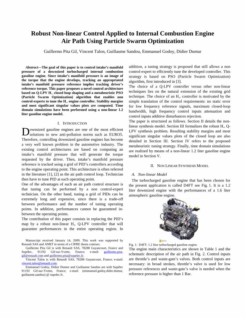
Abstract—The goal of this paper is to control intake’s manifold pressure of a downsized turbocharged internal combustion gasoline engine. Since intake’s manifold pressure is an image of the torque that the engine develops, tracking an appropriated intake’s manifold pressure reference implies tracking driver’s reference torque. This paper proposes a novel control architecture based on Q-LPV H∞ closed loop shaping and a metaheuristic PSO (Particle Swarm Optimization) algorithm that enables non control-experts to tune the H∞ engine controller. Stability margins and most significant singular values plots are computed. Time domain simulations have been performed using a non-linear 1.2 liter gasoline engine model.
I. INTRODUCTION
ownsized gasoline engines are one of the most efficient solutions to new anti-pollution norms such as EURO5.
Therefore, controlling downsized gasoline engines has become a very well known problem in the automotive industry. The existing control architectures are based on computing an intake’s manifold pressure that will generate the torque requested by the driver. Then, intake’s manifold pressure reference is tracked using a grid of PID’s controllers according to the engine operating point. This architecture is often referred in the literature [1], [2] as the air path control loop. Technician then have to tune PID at each operating point. One of the advantages of such an air path control structure is that tuning can be performed by a non control-expert technician. On the other hand, tuning a grid of PIDs can be extremely long and expensive, since there is a trade-off between performance and the number of tuning operating points. In addition, performances cannot be guaranteed in-between the operating points. The contribution of this paper consists in replacing the PID’s map by a robust non-linear H∞ Q-LPV controller that will guarantee performances in the entire operating region. In
Manuscript received January 14, 2009. This work was supported by
Renault SAS and ANRT in terms of a CIFRE thesis contract. Guillermo Pita Gil is with Renault SAS, 78288 Guyancourt, France and
Supélec, 91192 Gif-sur-Yvette, France; e-mail: [email protected] and [email protected].
Vincent Talon is with Renault SAS, 78288 Guyancourt, France; e-mail: [email protected].
Emmanuel Godoy, Didier Dumur and Guillaume Sandou are with Supélec 91192 Gif-sur-Yvette, France; e-mail: (emmanuel.godoy,dider.dumur, guillaume.sandou) @ supelec.fr.
addition, a tuning strategy is proposed that still allows a non control-expert to efficiently tune the developed controller. This strategy is based on PSO (Particle Swarm Optimization) algorithm, first introduced in [3]. The choice of a Q-LPV controller versus other non-linear techniques lies on the natural extension of the existing grid technique. The choice of an H∞ controller is motivated by the simple translation of the control requirements: no static error for low frequency reference signals, maximum closed-loop bandwidth, high frequency control inputs attenuation and control inputs additive disturbances rejection. The paper is structured as follows. Section II details the non-linear synthesis model. Section III formalizes the robust H∞ Q-LPV synthesis problem. Resulting stability margins and most significant singular values plots of the closed loop are also detailed in Section III. Section IV refers to the proposed metaheuristic tuning strategy. Finally, time domain simulations are realized by means of a non-linear 1.2 liter gasoline engine model in Section V.
II. NON LINEAR SYNTHESIS MODEL
A. Non-linear Model
The turbocharged gasoline engine that has been chosen for the present application is called D4FT see Fig. 1. It is a 1.2 liter downsized engine with the performances of a 1.6 liter atmospheric gasoline engine.
Fig. 1: D4FT: 1.2 liter turbocharged gasoline engine
The engine main characteristics are shown in Table 1 and the schematic description of the air path in Fig. 2. Control inputs are throttle’s and waste-gate’s valves. Both control inputs are necessary: in broad strokes, throttle’s valve is used for low pressure references and waste-gate’s valve is needed when the reference pressure is higher than 1 Bar.
Robust Non-linear Control Applied to Internal Combustion Engine Air Path Using Particle Swarm Optimization
Guillermo Pita Gil, Vincent Talon, Guillaume Sandou, Emmanuel Godoy, Didier Dumur
D

Fig. 2: D4FT’s air path scheme
The validation model of this engine, Fig.3, is available in ACHILLE’s library [1] and [4]. ACHILLE is a toolbox that has very detailed models of all Renault/Nissan gasoline and diesel engines. The model is 0D (no spatial dependency) and describes the complete air path: air filter, compressor, exchanger, turbine and catalyses. Fig. 4 shows an example of comparison between ACHILLE simulation results and real measurements of a full load transient response.
The non-linear model from where the synthesis Q-LPV model has been derived is based on the hypothesis that pressure varies
much faster than temperature and therefore temperature derivatives are neglected [5] and [6]. For the current application, intake’s manifold pressure and the pressure at the entry of the turbine have been kept as state variables:
( )
( )
−−=
−=
)(
)(
avtmavtmcylmavt
avt
colmapemcol
col
TQTQTQV
rP
dt
d
TQTQV
rP
dt
d
wgturbcylE
cylApap
(1)
where, by using a Bernoulli equation:
−=
−=
aptavtrTPeff
wgm
colaperT
Peffpapm
PPSQ
PPSQ
avt
avt
wg
ape
ape
pap
2
2
(2)
B. Q-LPV Polytopic Model
Q-LPV representations of non-linear models are not unique. An intuitive set of rules to choose the appropriate Q-LPV representation is:
− Respect the system nature (integrator, low-pass, etc.). − Do not make controller design harder. Avoid unstable
poles or zeros as far as possible. − Choose control inputs with a physical meaning.
According to these simple rules, a Q-LPV representation of the previously described gasoline engine model has been derived. Control inputs are chosen to be throttle’s valve and waste-gate’s valve efficient sections. By using these control inputs, we obtain a quasi-linear dependence of pressure derivatives with respect to control inputs while keeping their physical meaning.
TABLE II NOMENCLATURE
Symbol Signification
colP Intake’s manifold pressure
avtP Pressure at the entry of the turbine
aptP Pressure at the output of the turbine
papmQ Throttle’s valve mass flow
cylAmQ Cylinder’s mass flow
turbmQ Turbocharger’s mass flow
wgmQ Waste-gate’s valve mass flow
apeT Temperature after the heat exchanger
colT Intake’s manifold temperature
cylT Temperature in the cylinders
avtT Temperature at the entry of the turbine
colV Intake’s manifold volume
avtV Volume at the turbine entry
r Perfect gas constant
TABLE I ENGINE CHARACTERISTICS
Characteristic Value
Bore 69 mm Stroke 77 mm
Compression ratio 9.5 Number of cylinders 4
Fig. 4: Transient response of ACHILLE model. Red: measured, blue: model, green: model with a sensor (1st order)
Fig. 3: ACHILLE model of the D4FT

Regrouping non-linear terms as specified in (3) leads to the non-linear Q-LPV model (4).
=
−−
=
−=
−=
−=
avtcylcylE
aptavtrTP
avt
ape
avtavtavtturb
colaperT
P
col
ape
colavtcolcylA
VTQmrp
PPV
TrVPTQmr
PPV
TrVPTQmr
avt
avt
ape
ape
26
24
3
θ
θ
θ
θ
ε
(3)
+
=
effwg
effpap
avt
col
avt
col
S
S
p
P
P
P
P
dt
d
6
43
01
00
0
0
θθ
θθ
ε
(4)
Note that matrix B of the state space representation can be normalized as suggested in [7]. According to the present motor control application, the system dynamics are closed to actuators dynamics (which are first order-like with τpap and τwg time constants). Therefore, actuator’s dynamics need to be taken into consideration in the synthesis model (5).
+=+=
DuCxy
BuAxxɺ
(5)
where,
−−
=
=
=
=
−−
−−
0010000
0000001
00000
00000
001100
000010
,
11
11
3
6
4
2
1
wgwg
pappap
effwg
effpap
wg
pap
avt
col
DC
BA
S
S
p
u
u
p
u
x
x
P
P
x
ττττ
θθ
θθ
ε
with,
==⋅−<<⋅−
−<<−⋅<<⋅
−<<−
sec2.0
106984.5107963.3
798.575.71
10521.3104236.4
7688.084.47
96
11
104
93
wgpap ττθθθ
θ
ε
III. PROPOSED CONTROL ARCHITECTURE
In this section, H∞ Q-LPV controllers have been computed using H∞ Q-LPV techniques described in [8] and [9]. The following Fig. 5 closed-loop shaping filters structure has been used.
Control architectures with and without feed-forward actions and with and without measurable disturbance offer 4 different
trades-off between complexity and performance. For instance, when adding a feed-forward action, reference tracking is performed without overshoot. However, the controller has an additional entry, and therefore its B matrix an extra column.
Fig. 5: Q-LPV H∞ synthesis scheme
Note that there is a third varying parameter α that allows choosing whether the controller is going to use the waste-gate to perform reference tracking or not. Note also that because of including a varying parameter in the shaping filter W22(s), control input shaping filters have been placed after the actuators. This manipulation ensures that the synthesis problem can be expressed in terms of LMIs. Another way to overcome this difficulty could have been adding a sufficiently fast dynamic before the actuators. In our application, the first solution has been preferred to avoid higher order controllers. For the same reason, shaping filters k31, k32 and k4 have been chosen to be constants.
Most significant singular values plots have been computed Fig. 6 and compared to synthesis specified templates (dashed plot).
10-4
10-2
100
102
104
106
-60
-40
-20
0
20
10-4
10-2
100
102
104
106
-140
-100
-60
-20
20
60
10-4
10-2
100
102
104
106
-150
-100
-50
0
50
10-4
10-2
100
102
104
106
-200
-150
-100
-50
0
40
Frequency (rad/sec)
d1 e
t d2 t
o P
colr
ef-P
ref
(dB
)K
S t
o u
2 (
dB
)K
S t
o u
1 (
dB
)S
to P
colr
ef-P
col
(dB
)
Fig. 6: Main closed loop singular values
Quadratic stability has been successfully checked by finding a positive definite symmetric matrix X such that:
0looplosedloopclosed ≺T
icT
i XAXA −− +
−
Throttle
Waste Gate
00100
00001
1010
0100 3
εθθ
W1(s)
k4
k31 W21(s)
αW22(s)
),,( 3 αθθ εK
k32

is verified for all polytope’s vertexes. In addition, closed-loop poles at polytope’s vertexes Fig. 7 present good damping ratios.
-26 -24 -22 -20 -18 -16 -14 -12 -10 -8 -6 -4 -2 0 2-20
-15
-10
-5
0
5
10
15
20
Fig. 7: Closed loop poles of the equivalent LTI at the polytope’s vertexes.
In the simplest structure case (no feed-forward actions and no measurable disturbance, Nichols diagrams obtained by opening the loop at the measurement are plot in Fig. 8. Stability margins (50dB gain margin and 67° phase margin) are sufficient, since minimum requirements are 20 dB gain margin and 45° phase margin.
Open-Loop Phase (deg)
Open
-Loop G
ain(d
B)
-200 -190 -180 -170 -160 -150 -140 -130 -120 -110 -100 -90-70
-60
-50
-40
-30
-20
-10
0
10
20
30
40
50
60
70
Fig. 8: Nichols Diagrams of the Open loop.
Note also that the Bode diagrams of the equivalent frozen LTI at each vertex of the controller, Fig. 9, illustrate PI plus phase lead behavior.
0
20
40
60
80
-90-60-30
0306090
Pcol Pcol to first outputref m-
Frequency (rad/sec)
Phas
e (d
eg)
Mag
nit
ude
(dB
)
Pcol Pcol to second outputref m-
Frequency (rad/sec)
Phas
e (d
eg)
Mag
nit
ude
(dB
)
-40
-20
0
20
40
60
10-3
10-2
10-1
100
101
102
103
10-3
10-2
10-1
100
101
102
103
-180
-90
0
90
180
270
Fig. 9: Bode Diagram of the Controller at the vertexes of its polytope.
IV. CONTROL LAW TUNING
A. The Tuning Optimization Problem
Control law tuning has become a very important problem for industry applications. It is one of the main factors that are taken into consideration when choosing among all available control laws the most suited one for an industrial use. The purpose is to ensure that a non control-specialist user can “easily” tune the control law. In the current application, a metaheuristic optimization algorithm (with no tuning parameters) will choose the shaping filters (see [10]) that minimize a criterion built as follows:
)1exp(exp
exp
expexp)W(
margin
marginmargin
margin
marginmargin
max
max
max
max
Gain
GainGain
Phase
PhasePhase
−+
+
+
+
+
+
=
−
−
−−
opt
DDD
ttt
γ
J
Min
Min
%
%%
r
rr
(6)
Note that there are no weights in the criterion so that the person in charge of tuning the controller will only have to specify the maximum acceptable response time, the minimum acceptable gain margin, the minimum acceptable phase margin, the maximum acceptable overshoot, etc. Note also that adding the last term to the sum ensures that L2 gain is smaller than the unity if the final value of the criterion is smaller than one.
The decision variables are the parameters that define the shaping filters. For W1(s), W21(s) and W22(s), there are three parameters for each (since they are first order-like): low frequency gain, high frequency gain and the frequency for which the gain magnitude equals 0 dB; and in the case of k31, k32 and k4 just the values of the constants. Therefore, the total number of decision variables is 12.
B. Particle Swarm Optimization
Particle swarm Optimization (PSO) was firstly introduced in [3]. This optimization method is inspired by the social behavior of bird flocking or fish schooling.
Consider the following optimization problem: )(min xf
x χ∈ (7)
P particles are moving in the search space. Each of them has its own velocity, and is able to remember where it has found its best performance. Each particle has some “friends”. The following notations are used:
− kpx position of particle p at iteration k.
− kpv : velocity of particle p at iteration k.
− , 1
))(min(argkp
kp xbx
kp xfb
−∈= : best position found by particle p
until iteration k.
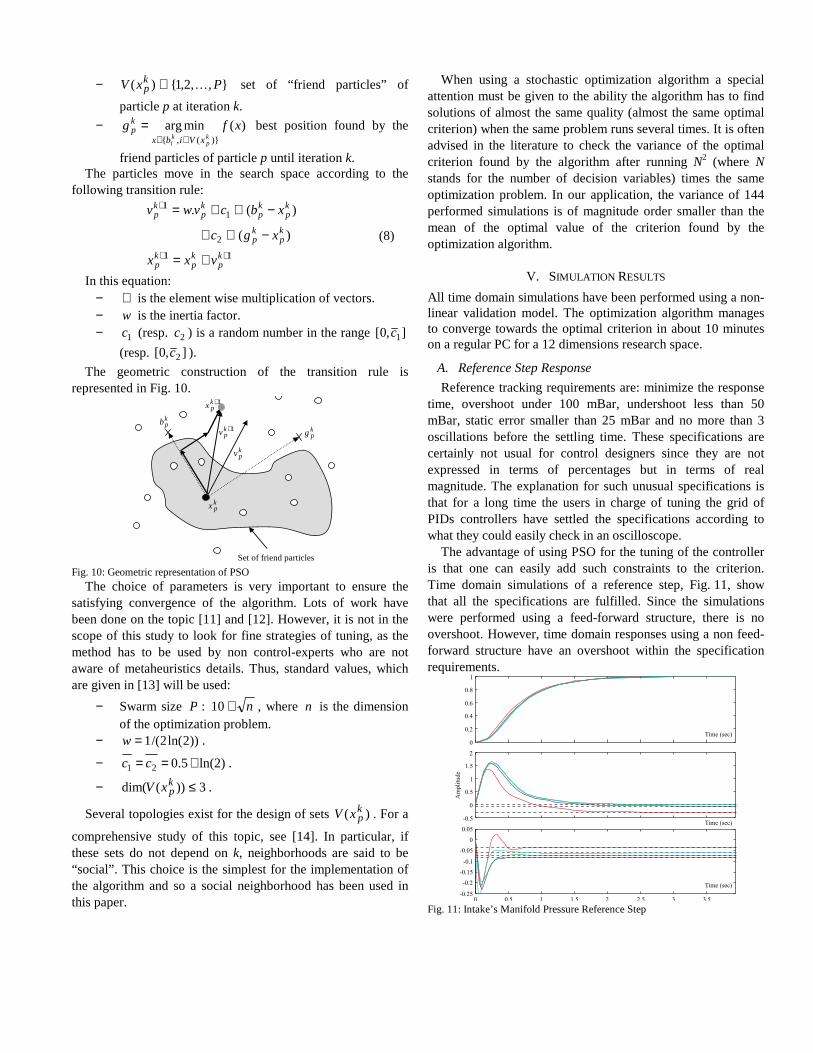
− ,,2,1)( PxV kp …⊂ set of “friend particles” of
particle p at iteration k.
− )(minarg)(,
xfgkp
ki xVibx
kp
∈∈= best position found by the
friend particles of particle p until iteration k. The particles move in the search space according to the
following transition rule:
11
2
11
)(
)(.
++
+
+=
−⊗+
−⊗+=
kp
kp
kp
kp
kp
kp
kp
kp
kp
vxx
xgc
xbcvwv
(8)
In this equation: − ⊗ is the element wise multiplication of vectors. − w is the inertia factor. − 1c (resp. 2c ) is a random number in the range ],0[ 1c
(resp. ],0[ 2c ).
The geometric construction of the transition rule is represented in Fig. 10.
Set of friend particles
kpb
kpg
kpx
kpv
1+kpv
1+kpx
Fig. 10: Geometric representation of PSO
The choice of parameters is very important to ensure the satisfying convergence of the algorithm. Lots of work have been done on the topic [11] and [12]. However, it is not in the scope of this study to look for fine strategies of tuning, as the method has to be used by non control-experts who are not aware of metaheuristics details. Thus, standard values, which are given in [13] will be used:
− Swarm size P : n+10 , where n is the dimension of the optimization problem.
− ))2ln(2/(1=w .
− )2ln(5.021 +== cc .
− 3))(dim( ≤kpxV .
Several topologies exist for the design of sets )( kpxV . For a
comprehensive study of this topic, see [14]. In particular, if these sets do not depend on k, neighborhoods are said to be “social”. This choice is the simplest for the implementation of the algorithm and so a social neighborhood has been used in this paper.
When using a stochastic optimization algorithm a special attention must be given to the ability the algorithm has to find solutions of almost the same quality (almost the same optimal criterion) when the same problem runs several times. It is often advised in the literature to check the variance of the optimal criterion found by the algorithm after running N2 (where N stands for the number of decision variables) times the same optimization problem. In our application, the variance of 144 performed simulations is of magnitude order smaller than the mean of the optimal value of the criterion found by the optimization algorithm.
V. SIMULATION RESULTS
All time domain simulations have been performed using a non-linear validation model. The optimization algorithm manages to converge towards the optimal criterion in about 10 minutes on a regular PC for a 12 dimensions research space.
A. Reference Step Response
Reference tracking requirements are: minimize the response time, overshoot under 100 mBar, undershoot less than 50 mBar, static error smaller than 25 mBar and no more than 3 oscillations before the settling time. These specifications are certainly not usual for control designers since they are not expressed in terms of percentages but in terms of real magnitude. The explanation for such unusual specifications is that for a long time the users in charge of tuning the grid of PIDs controllers have settled the specifications according to what they could easily check in an oscilloscope.
The advantage of using PSO for the tuning of the controller is that one can easily add such constraints to the criterion. Time domain simulations of a reference step, Fig. 11, show that all the specifications are fulfilled. Since the simulations were performed using a feed-forward structure, there is no overshoot. However, time domain responses using a non feed-forward structure have an overshoot within the specification requirements.
0
0.2
0.4
0.6
0.8
1
-0.5
0
0.5
1
1.5
2
0 0.5 1 1.5 2 2.5 3 3.5-0.25
-0.2
-0.15
-0.1
-0.05
0
0.05
Time (sec)
Time (sec)
Time (sec)
Am
pli
tud
e
Fig. 11: Intake’s Manifold Pressure Reference Step

B. Disturbance Step Response
Time domain responses to disturbance steps, Fig. 12 and 13, show that the controller manages to efficiently reject the additive disturbances on the control inputs: it has no static error and the response time is short enough.
0
0.2
0.4
0.6
0.8
1
-1
0
1
2
3
4
0-1
-0.5
0
0.5
1 2 3 4
Time (sec)
Fig. 12: Additive Disturbance Step on u1
0
0.2
0.4
0.6
0.8
1
-1
0
1
2
3
4
-1
-0.5
0
0.5
0 1 2 3 4
Time (sec)
Fig. 13: Additive Disturbance Step on u2
VI. CONCLUSIONS
This paper presents a new control structure to perform efficient reference tracking in the air path of a downsized turbocharged gasoline engine. The proposed H∞ Q-LPV control structure is computed using a closed-loop shaping
*design coupled with a metaheuristic PSO (Particle Swarm Optimization) algorithm that allows non control-experts to easily tune the engine controller.
Results are encouraging. Time domain simulations confirm that the resulting controller manages to fulfill all time-domain synthesis requirements in spite of a non-linear validation model.
VII. PERSPECTIVES
Future work will validate the proposed control architecture within a real D4FT engine and discuss onboard implementation requirements of the Q-LPV H∞ controller.
Robust anti-windup actions will be added to the control loop in order to minimize undesirable effects due to actuators saturations.
REFERENCES
[1] V. Talon, T. Tabet, S. Castric and P. Emery. “Engine control model based design with ACHILLE library”. E-COSM Rencontres Scientifiques de l’IFP. October 2006.
[2] G. Colin, Y. Chamaillard, A. Charlet, G. Bloch, G. Corde. Linearized Neural Predictive Control: A Turbocharged SI Engine Application. SAE 2005-01-0046.
[3] R.C. Eberhart, J. Kennedy, J., “A new optimizer using particle swarm theory”, Sixth International Symposium on Micromachine and Human Science, Nagoya, Japan. pp. 39-43, 1995.W.-K. Chen, Linear Networks and Systems (Book style). Belmont, CA: Wadsworth, 1993, pp. 123–135.
[4] G. Martin, V. Talon, P. Higelin, A. Charlet and C. Caillol. “Implementing turbomachinery physics into data map-based turbocharger models”. SAE 2009-01-0310.
[5] L. Guzzella and C. Onder. “Introduction to Modeling and Control of Internal Combustion Engine System”. Springer 2004.
[6] E. Hendricks and S. Sorenson. “Si engine controls and mean value modeling”. SAE paper No. 910258, 1991.
[7] P. Apkarian, P. Gahinet and G. Becker. “Self scheduled H control of linear parameter varying systems: a design example”. Automatica, 1995, n°31, pp 1251-1261..
[8] K. Zhou, J.C. Doyle, K. Glover, ”Robust and Optimal Control”. Prentice-Hall, 1996.
[9] G. Pita Gil, M. Ganet. “Gain-Scheduled and LPV Control for Re-entry Vehicle”. 7th international ESA Conference on Guidance, Navigation and Control, 2008.
[10] G. Sandou, G. Duc, D. Beauvois, “Optimisation par essaim particulaire du réglage d’un correcteur H-infini”, Actes de la 5ième Conférence Internationale Francophone d’Automatique internationale (2008) CD ROM 5ième Conférence Internationale Francophone d’Automatique (2008-09-03), Bucharest, Romania.
[11] Shi, Y., and Eberhart, R.C. (1998). Parameter selection in particle swarm optimization. : Proc. of the 7th Annual Conf. on Evolutionary Programming, USA, pp. 591-600.
[12] Eberhart, R.C., and Shi, Y. (2000). Comparing inertia weights and constriction factors in particle swarm optimization. In: Proc. of the IEEE Congress on Evolutionary Computation, San Diego, USA.
[13] Kennedy, J. and Clerc, M. (2006). Standard PSO. http://www.particleswarm.info/Standard_PSO_2006.c
[14] J. Kennedy, “Small worlds and mega-minds: effects of neighborhood topology on particle swarm performance”, IEEE Congress on Evolutionary Computation (CEC 1999), Piscataway, NJ, USA, pp. 1931-1938, 1999


![Processus aléatoires et applications · la derni`ere´egalit´e pouvant se montrer par un d´eveloppement limit´e de log[(1−λn/n)n]. Exemple 1.1.5. La probabilit´e de gagner](https://img.pdfslide.us/doc/110x75/5c03911e09d3f2ab198d3ae3/processus-aleatoires-et-applications-la-derniereegalite-pouvant-se-montrer.jpg)