Spatio-Temporal Image Correlation Spectroscopy:Extension to Three Dimensions and Application to

Biological Systems

Dominique Guillet

Department of Physics

McGill University, Montreal

Quebec, Canada

April 2012

A Thesis submitted to McGill University

in partial fulfillment of the requirements of the degree of

Master of Science

c© Dominique Guillet, 2012

Contents

Abstract vii

Resume viii

Statement of Originality ix

Acknowledgments x

1 Introduction 11.1 Fluorescence . . . . . . . . . . . . . . . . . . . . . . . . . . . . . . . . 21.2 Fluorescence Microscopy . . . . . . . . . . . . . . . . . . . . . . . . . 4

1.2.1 Confocal laser scanning microscopy (CLSM) . . . . . . . . . . 41.3 Fluorescence Correlation Spectroscopy . . . . . . . . . . . . . . . . . 61.4 Image Correlation Spectroscopy . . . . . . . . . . . . . . . . . . . . . 7

2 Spatiotemporal Image Correlation Spectroscopy 82.1 Image Correlation Techniques . . . . . . . . . . . . . . . . . . . . . . 8

2.1.1 Image Correlation Spectroscopy . . . . . . . . . . . . . . . . . 92.2 Spatio-Temporal Image Correlation Spectroscopy . . . . . . . . . . . 10

2.2.1 Immobile Population Removal . . . . . . . . . . . . . . . . . . 132.2.2 Experimental Limitations . . . . . . . . . . . . . . . . . . . . 14

3 Vesicle Dynamics during Plant Cell Cytokinesis 183.1 Biological System: Somatic Cytokinesis . . . . . . . . . . . . . . . . . 183.2 Materials and Methods . . . . . . . . . . . . . . . . . . . . . . . . . . 243.3 Results . . . . . . . . . . . . . . . . . . . . . . . . . . . . . . . . . . . 25

3.3.1 Vesicle dynamics . . . . . . . . . . . . . . . . . . . . . . . . . 253.3.2 Cell plate growth rate . . . . . . . . . . . . . . . . . . . . . . 29

3.4 Discussion . . . . . . . . . . . . . . . . . . . . . . . . . . . . . . . . . 31

4 Extension of STICS to 3 Dimensions 364.1 Theory . . . . . . . . . . . . . . . . . . . . . . . . . . . . . . . . . . . 374.2 Computer Simulations . . . . . . . . . . . . . . . . . . . . . . . . . . 40

4.2.1 3D simulator . . . . . . . . . . . . . . . . . . . . . . . . . . . 40

iii

iv CONTENTS

4.2.2 Simulation Results . . . . . . . . . . . . . . . . . . . . . . . . 43

5 Conclusion 55

References 58

List of Figures

1.1 Jablonski diagram . . . . . . . . . . . . . . . . . . . . . . . . . . . . . 31.2 Fluorescent spectra of two fluorescent proteins . . . . . . . . . . . . . 41.3 Schematic of a laser scanning confocal microscope . . . . . . . . . . . 51.4 Schematic representation of the image correlation spectroscopy technique 7

2.1 Evolution of the correlation function of a STICS analysis . . . . . . . 122.2 Image from a dividing plant cell with region of analysis overlayed . . 162.3 Evolution of the correlation function as a function of time lag . . . . 172.4 Example of a vector map from a STICS analysis . . . . . . . . . . . . 17

3.1 Sketch of vesicles and vesicle fusion with each other and the cell plate 193.2 Sketch of the different components of plant cell cytokinesis . . . . . . 203.3 Summary of the stages of cell division . . . . . . . . . . . . . . . . . . 233.4 Selected frames from a CLSM fluorescence image time series showing

the reorientation of the cell plate . . . . . . . . . . . . . . . . . . . . 253.5 STICS vector map during accumulation of vesicles . . . . . . . . . . . 263.6 STICS vector maps at different stages of cytokinesis . . . . . . . . . . 283.7 STICS vector map at the ring phragmoplast stage of cell division . . 293.8 Analysis of the growth rate of the cell plate . . . . . . . . . . . . . . 303.9 FRAP experiment on the cell plate of a dividing BY-2 cell . . . . . . 35

4.1 Schematic representation of a 3D image stack time series . . . . . . . 374.2 Contour plots of the 3D autocorrelation function . . . . . . . . . . . . 434.3 Contour plots of the time evolution of the 3D correlation function . . 444.4 3D STICS results for simulations with increasing velocity magnitudes

in the z dimension . . . . . . . . . . . . . . . . . . . . . . . . . . . . 464.5 Spatial spreading of the correlation function with movement . . . . . 474.6 3D STICS results of simulations for increasing values of flowing particle

density . . . . . . . . . . . . . . . . . . . . . . . . . . . . . . . . . . . 484.7 3D STICS results of simulations with velocity components in all three

spatial dimensions . . . . . . . . . . . . . . . . . . . . . . . . . . . . . 524.8 3D STICS results of simulations with flowing and filtered immobile

populations . . . . . . . . . . . . . . . . . . . . . . . . . . . . . . . . 53

v

List of Tables

4.1 Adjustable parameters for 3D simulations . . . . . . . . . . . . . . . 424.2 Comparison between STICS and 3D STICS results for simulations of

2D velocities . . . . . . . . . . . . . . . . . . . . . . . . . . . . . . . . 454.3 Effect of resolution and number of images in z on 3D STICS . . . . . 50

vi

Abstract

The object of this thesis is to present work done using spatio-temporal image correla-

tion spectroscopy (STICS), a technique that uses fluorescence intensity fluctuations in

a microscopy image time series to calculate a complete space-time correlation function

in order to measure transport dynamics in cells. The time evolution of this correla-

tion function gives information on the magnitude and direction of a flow of fluorescent

particles sampled in the image series. First, a new application of STICS to plant cell

biology is shown. In dividing plant cells, delivery of new cell wall material to the

forming cell plate requires intricate coordination of secretory vesicle trafficking and

delivery. In this work, STICS is used to measure vesicle dynamics during plant cell

division. It was discovered that vesicle transport to the plane of division occurs in

three phases, each with its characteristic flow patterns and range of velocities, which

directly reflect the rate of growth of the forming cell plate. The second part of this

thesis presents the extension of the STICS technique to a third spatial dimension. The

development of this new technique, called 3D STICS, allows the study of transport

dynamics in three dimensions, which is more relevant in tissues and non adherent cells

which are inherently 3D. Computer simulations were performed to test the accuracy

and precision of the technique under a range of parameters such as particle density of

immobile and moving populations; and number of images, velocity and resolution in

the third spatial dimension. A comparison between values of velocities in a 2D plane

recovered using STICS and its new 3D version is also presented.

vii

Resume

L’objet de cette these est de presenter des travaux faits a l’aide de la spectroscopie

par correlation spatiotemporelle d’images (STICS), une technique qui utilise les fluc-

tuations d’intensite dans une serie d’images capturees a l’aide d’un microsope par

fluorescence pour calculer la fonction complete de correlation spatiotemporelle, et

ainsi mesurer la dynamique du transport de proteines a l’interier de cellules vivantes.

L’evoultion temporelle de cette fonction de correlation donne de l’information sur

la direction et la vitesse d’un flot de particules fluorescentes presentes dans la serie

d’images. Tout d’abord, une nouvelle application de la technique en biologie vegetale

est presentee. Lors de la division cellulaire vegetale, le transport du materiel mem-

branaire necessaire a la formation de la plaque cellulaire requiert une grande precision

dans la coordination du transport et de la livraison des vesicules de secretion. Dans

cette these, STICS est utilisee pour mesurer la dynamique de ces vesicules pendant la

division cellulaire vegetale. Les resultats obtenus revelent l’existence de trois phases

dans le transport des vesicules de secretion au site de division cellulaire, chacune

presentant une echelle de vitesse et des motifs de mouvement characteristiques qui se

refletent dans le taux de croissance de la plaque cellulaire. Dans un deuxieme temps, le

developpement de STICS pour inclure l’analyse de la troisieme dimension spatiale est

presente. Cette nouvelle technique, appelee STICS 3D, permet l’etude de dynamiques

en trois dimensions, ce qui est plus pertinent que la version deux-dimensionnelle pour

les tissus et les cellules non adherentes, qui ont un environnement intrinsequement

3D. Des simulation par ordinateur ont ete effectuees pour determiner l’exactitude,

la precision et les limites de la technique pour un eventail de parametres comme la

vitesse, le nombre d’images et la resoultion dans la troisieme dimension spatiale ainsi

que la densite des populations immobiles et en mouvement. Une comparaison en-

tre les resultats obtenus avec STICS et la nouvelle version 3D de la technique est

egalement presentee.

viii

Statement of Originality

The author claims the following aspects of the thesis constitute original scholarship

and an advancement of knowledge:

Chapter 3 STICS measurements of vesicle dynamics during plant cell cytokinesis.

This chapter presents the first application of spatio-temporal image correla-

tion spectroscopy (STICS) on dividing plant cells and is the first comprehen-

sive characterization of endogenous secretory vesicle dynamics during plant cell

cytokinesis. Because of the interdisciplinary nature of this project, the work

presented was done in collaboration with Prof. Anja Geitmann’s group, from

Universite de Montreal. Chloe van Oostende performed cell culture, imaging,

FRAP experiments and analysis with FluMOS.

Chapter 4 Extension of STICS to 3 Dimensions. This chapter presents the devel-

opment of a new technique, 3D spatio-temporal image correlation spectroscopy

(3D STICS), which is an extension of STICS. This new technique allows the

study of transport dynamics in three dimensions, which is more relevant in tis-

sues and non adherent cells which are inherently 3D. This chapter presents the

theoretical basis of the technique as well as its characterization under various

simulation parameters.

ix

Acknowledgments

First I would like to thank my supervisor, Prof. Paul Wiseman, for giving me the

opportunity to be a part of his research group. It is thanks to him that I have ex-

perienced stimulating collaborations and leading-edge research. He has my gratitude

for giving me a chance as a simple undergraduate one summer and accepting me in

his group ever since.

I also want to acknowledge my research collaborators, without whom part of this

thesis would have never existed. First I need to thank Prof. Anja Geitmann, from

Universite de Montreal, for allowing me to work with her group on this interesting

project of dividing plant cells. I also have to recognize the incredible work of her

postdoc, Chloe van Oostende, who was a big part of this project, taking care of the

cell culture and imaging, and analyses of cells with FRAP and FluMOS. I have to

thank her for the numerous meetings and long - but always enjoyable! - discussions

that were necessary to obtain the results we have now.

I also need to thank many people from my own research group. Antoine Godin

helped me considerably with the coding of 3D STICS and the 3D simulator in MatLab.

I also have to thank Laurent Potvin-Trottier and Benjamin Rappaz for the stimulating

discussions around cups of coffee in the morning and for the training they gave me

in cell culture. Finally I have to thank all other Wiseman group members, present or

past, alongside whom I have worked. They have all contributed in their own way to

make my time in the group an enjoyable and priceless experience.

The final acknowledgements must go to my family, and especially to my parents,

Christiane and Jean-Pierre. They have instilled in me, ever since I was very young, a

thirst for knowledge and a wonderment of life. They have given me the confidence to

believe in myself and the drive to seek out challenges. They have always supported

me and have given me their unconditional love, for which I am forever grateful.

x

Chapter 1

Introduction

Despite being the smallest living organisms, cells are arguably amongst the most

important subject of study for human society since they form the basis of every

living thing. They interact together through extremely complex pathways using an

incredible variety of molecules to perform tasks like signalling, transport and cell

division, to name only a few. In spite of abundant research in the field since their

discovery hundreds of years ago, much still remains to be understood about the

functions and mechanisms of cells.

The emergence of new microscopy techniques to study the many different aspects

of cells and cell functions have advanced the field of biophysics in the last decade.

However, new quantitative analysis techniques also had to be developed to keep up

with the increasing quantity of data generated and to probe the system under study

at various spatial and time scales. Fluorescence fluctuation techniques are among

the most useful and versatile tools to have been established in recent years. One

such technique is called spatio-temporal image correlation spectroscopy (STICS), a

technique that extracts information from fluorescence fluctuations in an image time

series to map the movement of fluorescently labeled particles inside a living cell.

This thesis presents the application of STICS to a new biological system: the

dynamics of secretory vesicle in dividing plant cells. These vesicles are crucial to

1

2 CHAPTER 1. INTRODUCTION

the formation of the new cell wall: their transport to the proper location in the cell

at the right time is of utmost importance to the normal development of the plant.

As well, the extension of the technique to a third spatial dimension is presented, by

application to 3D image time series. This will allow the study of protein dynamics

in cells in a 3D environment, which is a more biologically relevant environment for

tissues.

This works will review, in Chapter 1, the fundamental concepts and experimental

techniques that are essential to the work done in this thesis. Then, Chapter 2 will

introduce the STICS technique: the theoretical basis behind it along with its strengths

and limitations. Chapter 3 will show the application of STICS to dividing plant cells

and the results obtained. This will be followed by Chapter 4, where the extension

of the technique to three spatial dimensions is presented. The final chapter will give

a summary of the work and discuss potential future research projects based on this

work.

1.1 Fluorescence

The field of live cell biology took a giant leap forward when the naturally occurring

green fluorescent protein (GFP) was extracted and purified for the first time from the

jellyfish Aequorea victoria [1]. Indeed, this was a breakthrough because it became

possible to have the cell synthesize a protein of interest attached with a GFP fluo-

rescent maker by genetically splicing the GFP codon within the genetic code of the

protein. This revolutionized live cell imaging. Since its discovery, many mutants have

been made that fluoresce at different wavelengths, making fluorescent proteins a ver-

satile tool for fluorescence microscopy, one of the most widely used imaging technique

in the field of biology.

Fluorescence occurs when a molecule in a singlet excited state rapidly returns to

the ground singlet state via the emission of a photon of a longer wavelength than

1.1. FLUORESCENCE 3

that of the photon that was originally absorbed by the molecule to excite the elec-

tron [2]. Fluorescence can be explained with Jablonski diagrams, named after Alexan-

der Jablonski, who introduced them as a representation of electronic energy levels [3].

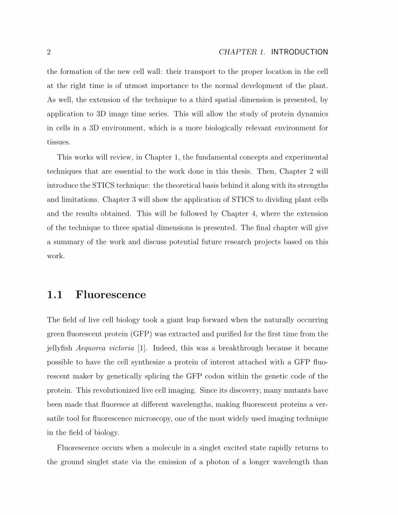
Figure 1.1: Jablonski diagram showing the different energy levels

Figure 1.1 is an example of such a diagram. Initially, the molecule is in the ground

state S0. Upon absorbing a photon of excitation light, electrons can be promoted to

the first excited singlet state S1. This process occurs very rapidly, on the femtosecond

time scale. After absorption, the molecule is in a high vibrational state of the singlet

excited state. It rapidly relaxes to the lowest vibrational state level of S1 through a

non-radiative decay process, on the time scale of 10−12 s. When the molecule drops

from the lowest vibrational excited state back to the ground state, a photon is emitted

as fluorescence emission on the nanosecond time scale. Some energy is lost by the

molecule during the vibrational relaxation, so the absorbed and emitted photons dif-

fer in wavelength. This shift of the emission to longer wavelength is called the Stokes

shift. It is essential for fluorescence microscopy, as it allows the simultaneous exci-

tation and detection of fluorescent molecules by using optical filters to block out the

excitation light and detect the weaker fluorescence emission. Each fluorescent protein

4 CHAPTER 1. INTRODUCTION

has its own characteristic absorption-emission spectrum. This allows the observation

of more than one fluorescent population at the same time, if they have sufficiently

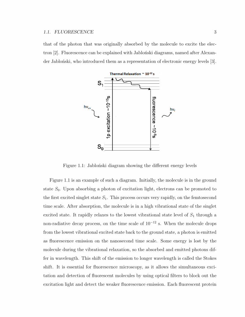
different emission wavelength peaks. An example of the spectra of enhanced green

fluorescent protein (EGFP) and MitoTracker Orange is shown in Figure 1.2.

Figure 1.2: Absorption (dotted line) and fluorescence emission (full line) spec-

tra of EGFP (green) and MitoTracker Orange (blue). Data available from

www.invitrogen.com

1.2 Fluorescence Microscopy

Fluorescence microscopes make use of the principles of fluorescence described in the

previous section to excite a sample labelled with a fluorescent marker and image the

fluorescence emission at a different wavelength. Many different types of fluorescence

microscopes exist, using more or less complicated setups. The research presented in

this thesis mainly made use of confocal laser scanning microscopes.

1.2.1 Confocal laser scanning microscopy (CLSM)

The spatial resolution of any microscope is defined by the physical dimension of the

imaged diffraction pattern of a single point source, which is called the point spread

function (PSF). The degree of spreading in space of this PSF reflects on the quality

of an optical system.

1.2. FLUORESCENCE MICROSCOPY 5

Figure 1.3: Schematic of a laser scanning confocal microscope. Image reproduced

from [5]

The principal advantage of the confocal microscope, invented in 1957 by Marvin

Minsky [4], is to use a pin-hole to spatially filter out-of-focus light for samples thicker

than the PSF. This allows the imaging of thin cross-sections of a sample since flu-

orescence is only detected from a small illumination volume defined by the spatial

extent of the PSF. This also reduces blurring due to scattered light and improves the

signal-to-noise ratio. Furthermore, a confocal laser scanning microscope can raster

scan the sample point-by-point with a focused laser beam and reconstruct the fluores-

cence image using a computer. A schematic of a laser scanning confocal microscope

is shown in Fig 1.3.

In a CLSM, the laser beam is usually scanned across a sample using a set of

mirrors. Lenses collimate the beam, which passes through a dichroic mirror before

being focused by an objective lens into a small focal volume on or within the sample.

By scanning the focal point across the sample, the fluorophores in the focus are ex-

cited sequentially as the beam is scanned across the sample. Fluorescence emitted is

collected back through the same objective (epi mode) or the dichroic mirror, which

reflects the fluorescence emission into a CCD or PMT detector. Fluorophores slightly

below or above the focal plane may also be excited. This creates background fluores-

cence which reduces the signal-to-noise ratio. This background can be decreased with

6 CHAPTER 1. INTRODUCTION

a series of pinholes. The size of the PSF at the focal point is reduced by bringing

the excitation beam through a first pinhole. The emission signal passes through a

second pinhole in order to block the out-of-focus components along the edge of the

beam (see Figure 1.3) [6].

1.3 Fluorescence Correlation Spectroscopy

Many quantitative fluorescence techniques have been developed based on fluorescence

microscopy. One of the earliest fluorescence fluctuation techniques introduced is called

fluorescence correlation spectroscopy (FCS). Such time signal-correlation techniques

were first applied in the early 1970’s at Cornell University [7]. FCS essentially looks

at the intensity fluctuations arising from fluorescent particles moving into and out of

a small stationnary laser beam focus within a sample. FCS records these fluorescence

intensity fluctuations as a time series that is then used to calculate a temporal au-

tocorrelation function (see Figure 1.4). Information about the transport dynamics,

number of molecules and chemical reaction rates, for example, can be extracted from

the magnitude and characteristic time scale of the intensity fluctuations. Although

it has high time resolution, it is important to note that FCS measurements are made

only at a single point in space. Furthermore, results depend strongly on the size and

shape of the focal volume. The time scales involved in FCS range from microseconds

to milliseconds, making it possible to probe reactions and dynamics on short time

scales within the sample. However, extended exposure times can photobleach the

fluorescent labels under study and thus prevent the study of long timescale dynam-

ics. Many extensions of FCS have been developed over the years to tackle different

challenges [8]. The main technique of interest for this thesis is an imaging analog of

FCS called image correlation spectroscopy.

1.4. IMAGE CORRELATION SPECTROSCOPY 7

Figure 1.4: Schematic representation of the image correlation spectroscopy technique.

A) The fluorescence intensity is collected from the focal volume. Intensity fluctua-

tions arise from fluorophores moving in and out of the volume. B) The fluorescence

intensity is recorded as a function of time. The temporal autocorrelation function

will be calculated from this time series and reveal information on the dynamics of the

fluorescent molecules in the system.

1.4 Image Correlation Spectroscopy

Image correlation spectroscopy (ICS) differs from FCS in that it analyzes intensity

fluctuations sampled in space across an image recorded using a fluorescence micro-

scope instead of sampling in time from a fixed position in space. It can be thought

of as its spatial equivalent. The technique was first developed to look at aggregation

states and protein surface densities in cells [9]. The technique was later extended to

temporal ICS by calculating the time autocorrelation function from an image time

series [10]. Using both spatial and temporal correlation functions, ICS can recover

information about degree of aggregation, concentration, diffusion coefficients and dy-

namics of proteins. A more rigorous introduction to ICS will be presented in the next

chapter.

Chapter 2

Spatiotemporal Image Correlation

Spectroscopy

This thesis focuses on work done using spatio-temporal image correlation spectroscopy

(STICS), a technique developed in 2005 by Hebert et al. [11] as an extension of image

correlation spectroscopy (ICS) which was briefly introduced in the previous chapter.

STICS calculates a full space-time correlation function from the intensity fluctuations

in a fluorescence microscopy image time series. The time evolution of this correlation

function gives information on the magnitude and direction of a flow of fluorescent

particles sampled in the image series. This chapter will first present an introduction

to ICS, followed by a more in-depth review of STICS.

2.1 Image Correlation Techniques

All image correlation techniques are based on one common principle: calculating

the correlation function of intensity fluctuations recorded within a microscopy image

time series. They differ in the way they treat this data. Consider the generalized

correlation function,

8

2.1. IMAGE CORRELATION TECHNIQUES 9

rab(ξ, η, τ) =〈δia(x, y, t)δib(x+ ξ, y + η, t+ τ)〉〈ia(x, y, t)〉t〈ib(x, y, t+ τ)〉t+τ

(2.1)

where ξ and η are spatial lag variables and τ is the temporal lag variable. δi(x, y, t)

represents the intensity fluctuation of a pixel at position (x,y) and at time t and is

given by

δi(x, y, t) = i(x, y, t)− 〈i〉t (2.2)

where i(x, y, t) is the intensity at pixel (x, y) recorded in the image at time t. 〈i〉tis the average intensity of that image. The angular brackets in the numerator of

Eq. 2.1 represent an ensemble average of pixel intensity fluctuations over all pairs of

images separated by τ . The subcripts a and b refer to the general case of two detection

channels. By making different approximations to this generalized correlation function,

image correlation techniques can extract various information contained within the

image time series.

The correlation techniques described in this chapter make use of the microscope

point-spread function (PSF) to correlate fluorescence intensity fluctuations over space,

time, or both. Indeed, each image from a fluorescence microscope is the result of the

spatial convolution of the PSF with the location of all fluorescent point-emitters.

For spatial correlation, it is important for the signal from each point-source to be

oversampled: the convolution causes the integrated emission to be spread over a

number of adjacent pixels in the image, to an extent dependent on the size of the

PSF and the pixel size.

2.1.1 Image Correlation Spectroscopy

Taking τ = 0 in Eq. 2.1 reduces the problem to calculating and fitting the spatial

autocorrelation function for each separate frame. This corresponds to the original

technique called image correlation spectroscopy (ICS). The correlation function of

the image frame at time t is well approximated as a two-dimensional Gaussian:

10 CHAPTER 2. SPATIOTEMPORAL IMAGE CORRELATION SPECTROSCOPY

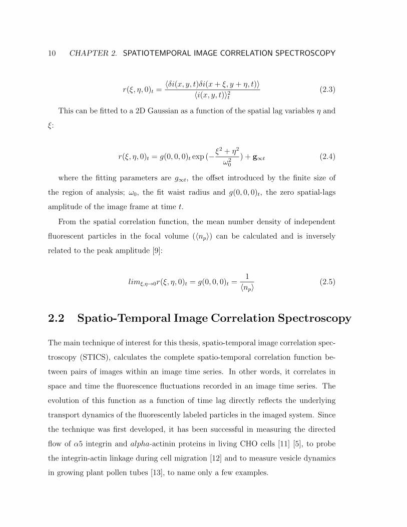
r(ξ, η, 0)t =〈δi(x, y, t)δi(x+ ξ, y + η, t)〉

〈i(x, y, t)〉2t(2.3)

This can be fitted to a 2D Gaussian as a function of the spatial lag variables η and

ξ:

r(ξ, η, 0)t = g(0, 0, 0)t exp (−ξ2 + η2

ω20

) + g∞t (2.4)

where the fitting parameters are g∞t, the offset introduced by the finite size of

the region of analysis; ω0, the fit waist radius and g(0, 0, 0)t, the zero spatial-lags

amplitude of the image frame at time t.

From the spatial correlation function, the mean number density of independent

fluorescent particles in the focal volume (〈np〉) can be calculated and is inversely

related to the peak amplitude [9]:

limξ,η→0r(ξ, η, 0)t = g(0, 0, 0)t =1

〈np〉(2.5)

2.2 Spatio-Temporal Image Correlation Spectroscopy

The main technique of interest for this thesis, spatio-temporal image correlation spec-

troscopy (STICS), calculates the complete spatio-temporal correlation function be-

tween pairs of images within an image time series. In other words, it correlates in

space and time the fluorescence fluctuations recorded in an image time series. The

evolution of this function as a function of time lag directly reflects the underlying

transport dynamics of the fluorescently labeled particles in the imaged system. Since

the technique was first developed, it has been successful in measuring the directed

flow of α5 integrin and alpha-actinin proteins in living CHO cells [11] [5], to probe

the integrin-actin linkage during cell migration [12] and to measure vesicle dynamics

in growing plant pollen tubes [13], to name only a few examples.

2.2. SPATIO-TEMPORAL IMAGE CORRELATION SPECTROSCOPY 11

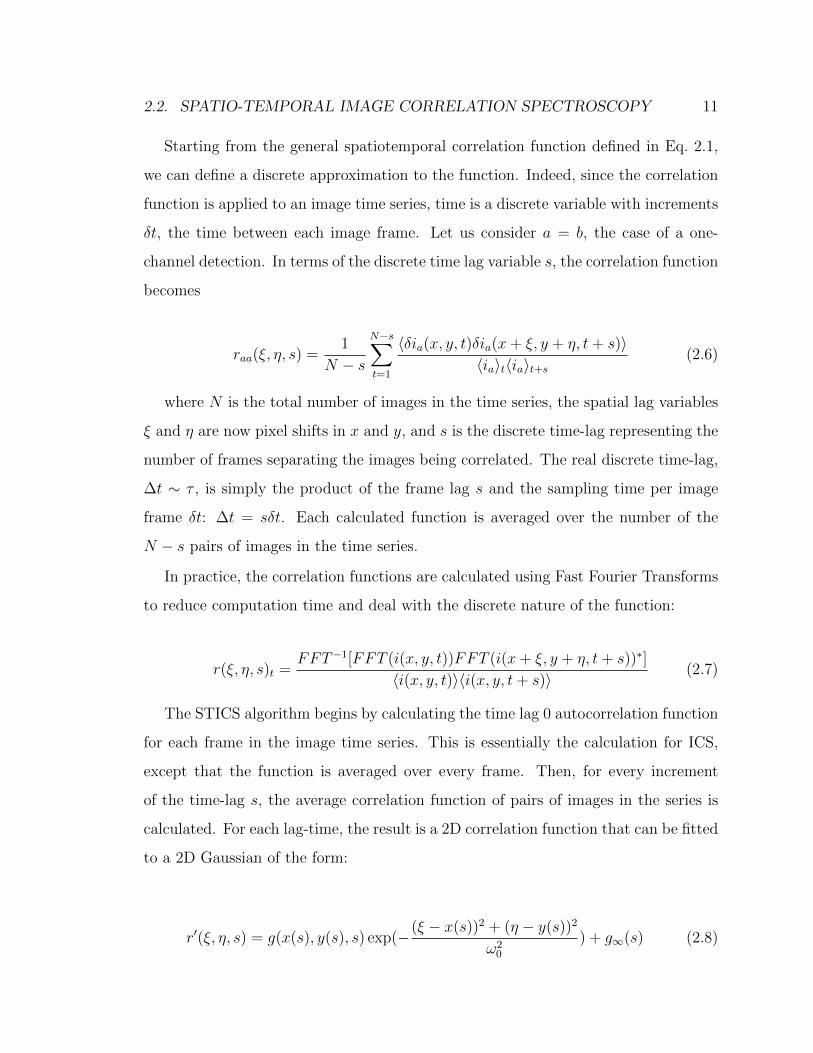
Starting from the general spatiotemporal correlation function defined in Eq. 2.1,

we can define a discrete approximation to the function. Indeed, since the correlation

function is applied to an image time series, time is a discrete variable with increments

δt, the time between each image frame. Let us consider a = b, the case of a one-

channel detection. In terms of the discrete time lag variable s, the correlation function

becomes

raa(ξ, η, s) =1

N − s

N−s∑t=1

〈δia(x, y, t)δia(x+ ξ, y + η, t+ s)〉〈ia〉t〈ia〉t+s

(2.6)

where N is the total number of images in the time series, the spatial lag variables

ξ and η are now pixel shifts in x and y, and s is the discrete time-lag representing the

number of frames separating the images being correlated. The real discrete time-lag,

∆t ∼ τ , is simply the product of the frame lag s and the sampling time per image

frame δt: ∆t = sδt. Each calculated function is averaged over the number of the

N − s pairs of images in the time series.

In practice, the correlation functions are calculated using Fast Fourier Transforms

to reduce computation time and deal with the discrete nature of the function:

r(ξ, η, s)t =FFT−1[FFT (i(x, y, t))FFT (i(x+ ξ, y + η, t+ s))∗]

〈i(x, y, t)〉〈i(x, y, t+ s)〉(2.7)

The STICS algorithm begins by calculating the time lag 0 autocorrelation function

for each frame in the image time series. This is essentially the calculation for ICS,

except that the function is averaged over every frame. Then, for every increment

of the time-lag s, the average correlation function of pairs of images in the series is

calculated. For each lag-time, the result is a 2D correlation function that can be fitted

to a 2D Gaussian of the form:

r′(ξ, η, s) = g(x(s), y(s), s) exp(−(ξ − x(s))2 + (η − y(s))2

ω20

) + g∞(s) (2.8)

12 CHAPTER 2. SPATIOTEMPORAL IMAGE CORRELATION SPECTROSCOPY

where g(x(s), y(s), s) is the peak intensity, x(s) and y(s) are the x and y coordi-

nates of the peak position, ω0 is the e−2 waist radius and g∞ is the spatial lag offset

of the correlation function. Following the evolution of the fit values as a function

of time lag can reveal information about the dynamics of the fluorescent population.

Indeed, the peak’s position is directly related to the flow of the particles. Therefore,

if the fluorescent population is undergoing directed flow, the correlation function’s

peak position will shift according to its magnitude and direction. On the other hand,

tracking the width of the peak will give information about the diffusion coefficient of

the particles. Some idealized cases are shown in Figure 2.1 calculated from computer

simulations of an image series.

Figure 2.1: STICS analysis of computer simulated images for different dynamics: i)

Directed flow. The peak moves in the direction opposite to the flow. ii) Diffusion. The

peak stays centered and progressively widens. iii) Directed flow and diffusion. The

peak divides in two parts, each presenting the behaviour of either diffusion (central

peak) or flow (translating peak). Image adapted from [11].

Once we have extracted the fit values of x(s) and y(s), we can recover the mag-

nitude and direction of the flow by calculating the velocity vectors vx and vy, given

that we know the pixel size and the time δt between each frame:

2.2. SPATIO-TEMPORAL IMAGE CORRELATION SPECTROSCOPY 13

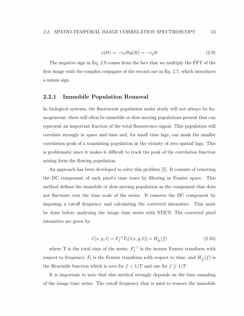
x(δt) = −vxδty(δt) = −vyδt (2.9)

The negative sign in Eq. 2.9 comes from the fact that we multiply the FFT of the

first image with the complex conjugate of the second one in Eq. 2.7, which introduces

a minus sign.

2.2.1 Immobile Population Removal

In biological systems, the fluorescent population under study will not always be ho-

mogeneous: there will often be immobile or slow-moving populations present that can

represent an important fraction of the total fluorescence signal. This population will

correlate strongly in space and time and, for small time lags, can mask the smaller

correlation peak of a translating population in the vicinity of zero spatial lags. This

is problematic since it makes it difficult to track the peak of the correlation function

arising form the flowing population.

An approach has been developed to solve this problem [5]. It consists of removing

the DC component of each pixel’s time trace by filtering in Fourier space. This

method defines the immobile or slow-moving population as the component that does

not fluctuate over the time scale of the series. It removes the DC component by

imposing a cutoff frequency and calculating the corrected intensities. This must

be done before analyzing the image time series with STICS. The corrected pixel

intensities are given by:

i′(x, y, t) = F−1f Ft(i(x, y, t))×H 1T

(f) (2.10)

where T is the total time of the series, F−1f is the inverse Fourier transform with

respect to frequency, Ft is the Fourier transform with respect to time, and H 1T

(f) is

the Heaviside function which is zero for f < 1/T and one for f ≥ 1/T .

It is important to note that this method strongly depends on the time sampling

of the image time series. The cutoff frequency that is used to remove the immobile

14 CHAPTER 2. SPATIOTEMPORAL IMAGE CORRELATION SPECTROSCOPY

component is defined by the Heaviside function H 1T

(f) and depends on the total time

T of the series. Filtering an image time series that is shorter in time will result in a

higher cutoff frequency, meaning more signal - and thus more information - will be

lost. It is therefore important to keep this in mind when comparing STICS results

for different image time series on which the Fourier filter was first applied. If there si

a distribution of velocities, the comparison will only be meaningful if the same time

sampling was used for all image time series.

2.2.2 Experimental Limitations

With correlation techniques, there is a lower limit on the sampling required in order

to have enough averaging of the correlation function to obtain reliable and meaningful

results. The accuracy and precision of ICS was investigated [14] and it was found that

the smallest usable region of interest (ROI) for ICS analysis was a region of 16x16

pixels2 area for typical imaging with a high NA objective lens. The same limit is

applicable to STICS. However, it suffers an additional restriction: since it calculates

the velocity of particles by tracking the translating peak of the correlation function,

the latter needs to stay in the ROI for a minimum of one time lag. This imposes an

upper limit to the velocities that can be recovered using this technique. Taking the

x-axis as an example, the maximal velocity that can be measured is

vmaxx =Nx × δx2× δt

(2.11)

where Nx is the size of the region in pixels, δx is the spatial resolution in µm per

pixel and δt is the time between image frames. The same equation is applicable to

the y axis. When analyzing data, the ROI chosen would usually have a size of a

16x16 pixels2 area, in order to obtain relatively finely sampled vector maps across a

cell. Therefore, the imaging rate has to be adjusted to fit the flow rate of the system

under study. A system that reaches high velocities will have to be imaged at a much

higher time resolution than a slower system.

2.2. SPATIO-TEMPORAL IMAGE CORRELATION SPECTROSCOPY 15

The STICS analysis is performed on image time series using a software first written

in Matlab by David Kolin of the Wiseman lab in 2007 and improved by various group

members since then. Some parameters have to be set in order to perform the analysis.

The user has to choose the maximum time lag τ over which the fluctuations are

correlated. The size of the analysis ROI’s also has to be set, with a minimum size of

16x16 pixels2 area as mentioned previously. The spacing between each ROI can also

be adjusted. If a spacing smaller than the subregion size is chosen, the subregions will

overlap. If they do, the velocity vectors from adjacent regions are not independent

of each other: hence there should be a certain continuity from one region to another.

The user can set a vector mismatch threshold to filter out vectors that deviate from

their neighbour by a certain amount.

The software ensures the reliability of the results obtained by implementing other

parameters that will stop the analysis for a specific subregion if a threshold value is

reached. For example, the user can set a beam radius threshold in µm that sets the

maximum e−2 radius allowed for the correlation functions. Another parameter is the

correlation local maxima, which is the ratio of the noise correlation peak amplitudes

(off center) to the amplitude of the correlation function from the fluctuation signal.

This ensures that the noise correlation peaks are not larger than the signal correlation

peak.

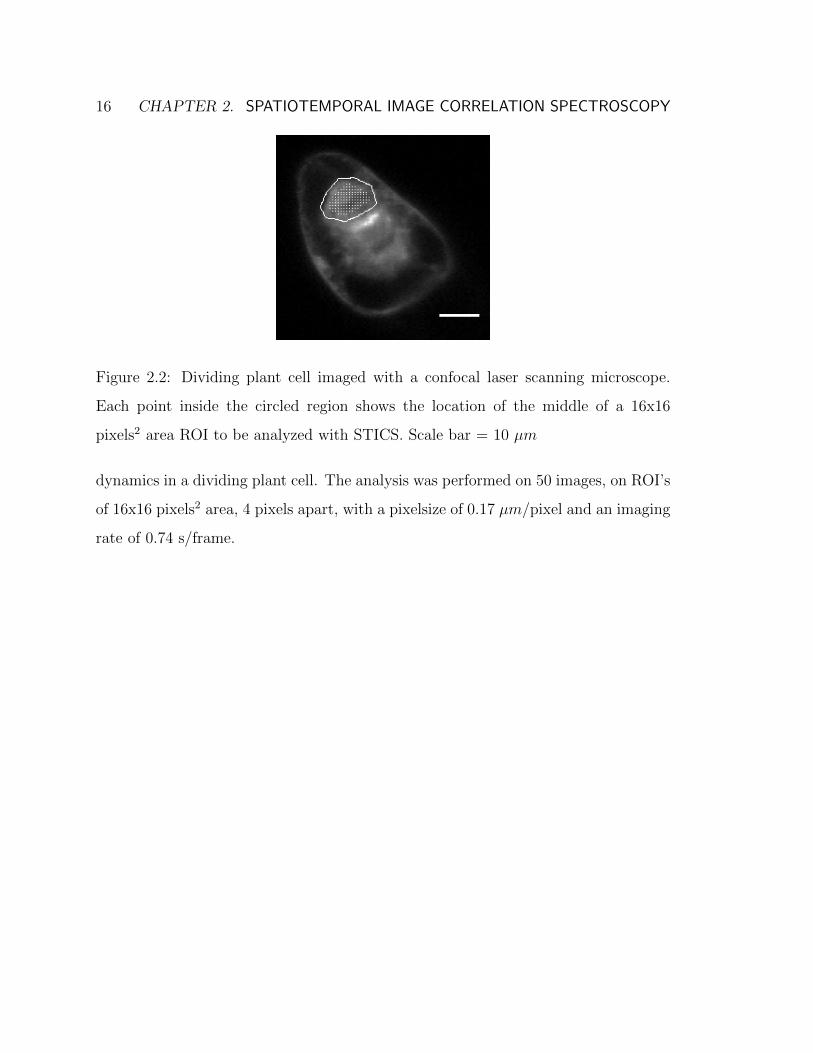
An example of the STICS technique applied to real experimental data is presented

here. Figure 2.2 shows the first image of the series with the region chosen to perform

the STICS analysis overlayed. The data presented is taken from a dividing plant

cell with secretory vesicles labeled with Knolle-GFP. This biological system and its

analysis with STICS will be the subject of the next chapter.

Figure 2.3B shows the time evolution of the correlation function for the suared

16x16 pixels2 ROI in Figure 2.3A. Figure 2.4 shows the resulting flow vectors for this

region and a few neighbouring ones, which were shown in Figure 2.2, overlayed on the

first image of the time series. These vectors give quantitative information on vesicle

16 CHAPTER 2. SPATIOTEMPORAL IMAGE CORRELATION SPECTROSCOPY

Figure 2.2: Dividing plant cell imaged with a confocal laser scanning microscope.

Each point inside the circled region shows the location of the middle of a 16x16

pixels2 area ROI to be analyzed with STICS. Scale bar = 10 µm

dynamics in a dividing plant cell. The analysis was performed on 50 images, on ROI’s

of 16x16 pixels2 area, 4 pixels apart, with a pixelsize of 0.17 µm/pixel and an imaging

rate of 0.74 s/frame.

2.2. SPATIO-TEMPORAL IMAGE CORRELATION SPECTROSCOPY 17

Figure 2.3: A) Close-up of the circled region in Figure 2.2. The square shows the

location of a ROI on which STICS is applied. Scale bar = 10 µm. B) Evolution of

the correlation function as a function of time lag shown for the squared region. For

each time lag, the correlation function is fitted to a 2D Gaussian function and the

time evolution of the peak’s location gives the magnitude and direction of the flow of

vesicles. Scale bar = 1 µm.

Figure 2.4: Resulting vector map for the STICS analysis of the ROI’s shown in

FIgure 2.2, which gives information on vesicle dynamics in a dividing BY-2 plant cell.

Scale bar = 10 µm.

Chapter 3

Vesicle Dynamics during Plant Cell

Cytokinesis

This chapter will discuss a new application of STICS to study the phenomenon of cell

division in plant cells. Here, STICS was used to measure the dynamics of secretory

vesicles carrying new cell wall material in plant cells undergoing somatic cytokinesis.

The high density and small size of the vesicles make this a perfect candidate for STICS

measurement. This chapter will first introduce the biological process studied, the

experimental techniques are then presented, followed by the results and a discussion

on their meaning.

3.1 Biological System: Somatic Cytokinesis

In eukaryotic cells, the cell cycle is divided into two main phases: interphase and

mitosis. Interphase is the longest of the two, and is itself divided in three stages: G1,

S and G2. G1 and G2 are two growth phases, while S in the stage at which the DNA

replicates in the cell. Mitosis, or M phase, is the relatively brief but complex period

when nuclear division occurs (karyokinesis). It is divided into five stages: prophase,

metaphase, anaphase, telophase and finally cytokinesis, in which the cytoplasm of

18

3.1. BIOLOGICAL SYSTEM: SOMATIC CYTOKINESIS 19

the cell is divided in two to form two daughter cells [15].

In plant cells, cytokinesis occurs when a cell plate forms in the middle of the cell,

expands in a centrifugal direction and attaches to the parent cell wall, thus physically

dividing the cytoplasm of the cell. The material components of the cell plate, like

pectins, hemicelluloses, callose and cellulose synthesizing enzyme complexes [16], are

delivered by secretory vesicles produced by Golgi stacks in the cell that fuse with the

cell plate. Figure 3.1 represents vesicles produced by the Golgi apparatus delivering

material components to the cell plate and fusing with each other and with the cell

plate during its formation.

Figure 3.1: Sketch representing vesicles produced by the Golgi apparatus delivering

material components to the cell plate and fusing with each other and with the cell

plate during its formation. Adapted from [5]

The vesicles need to be transported rapidly and efficiently to precise locations in

the cell at specific times in order for cell division to occur normally. Indeed, failure to

do so will result in abnormal growth patterns or aberrant deposition of the cell wall

components, or in the extreme, a complete absence of both processes [17]. Knowledge

about the dynamics between the production of the vesicles by Golgi stacks and their

fusion with the cell plate - the vesicle movements within the cytoplasmic space and

their method of delivery to the cell plate - is scarce. Measurement of the vesicles

20 CHAPTER 3. VESICLE DYNAMICS DURING PLANT CELL CYTOKINESIS

dynamics is the subject of investigation of the work presented in this chapter.

The new cell plate forms in the equatorial plane of a cytoskeletal array known as

the phragmoplast. This consists of opposing actin filaments and microtubules with

their (+) end facing the plane of division. The major function of the microtubules is

to deliver the Golgi-derived vesicles to the site of cell plate assembly in the center of

the structure, while the main role of the actin filaments is to guide the cell plate to

the proper site of fusion with the cell wall. [17]

Another distinct structure of plant cell cytokinesis is the cell plate assembly ma-

trix (CPAM). It is a transient, membrane-less cytoplasmic domain that encompasses

the vesicles fusing to form the cell plate. It is composed of various scaffolding, enzy-

matic, structural and regulatory proteins necessary for the formation of the cell plate

and these are transported to the assembly region by microtubules from the phragmo-

plast. [18] [19] The cell plate arises within the CPAM and undergoes a maturation

process throughout its formation, which takes typically approximately 30 minutes [20].

A sketch of the components of plant cytokinesis during cell plate formation is shown

in Figure 3.2.

Figure 3.2: Sketch of the different components of plant cell cytokinesis in the telophase

stage of cell division. Phragmoplast microtubules direct vesicles from Golgi stacks to

the site of fusion with the cell plate, which is expanding outwards.

The Golgi stacks that produce the secretory vesicles are known to accumulate

3.1. BIOLOGICAL SYSTEM: SOMATIC CYTOKINESIS 21

at the equatorial plane in a belt-shaped arrangement. Although the Golgi stacks

are close to the phragmoplast, they are excluded from it [21]. The mean distance

between the bulk of the Golgi stacks and the destination sites of the vesicles in the

equatorial plane is usually several micrometers and about 5-10 µm in the BY-2 cells

studied. Golgi stack dynamics and the eventual fusion of vesicles in the equatorial

plane have been extensively investigated by optical as well as transmission electron

microscopy [22] [23]. It is interesting to note that taking into account the average

diameter of a new cell wall (∼ 9 µm), the mean number of Golgi stacks per cell (∼

68 during mitosis [21]), the dimension of Golgi-derived vesicles (∼ 50 nm [20]) and

the fact that about 30% of the cell plate membrane is recycled by vesicles during

maturation [20], each Golgi stack must produce on average 310 vesicles to form the

new cell wall. It is believed that most vesicles are transported to the site of cell plate

assembly in 6 to 8 minutes (from metaphase to the early stage of karyokinesis) [24].

Such estimates show that there must be a high degree of vesicle trafficking during

that period of time.

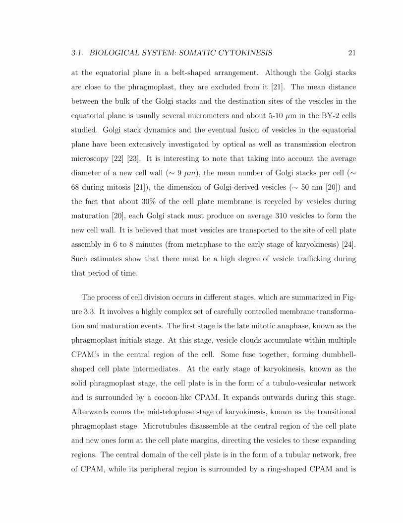
The process of cell division occurs in different stages, which are summarized in Fig-

ure 3.3. It involves a highly complex set of carefully controlled membrane transforma-

tion and maturation events. The first stage is the late mitotic anaphase, known as the

phragmoplast initials stage. At this stage, vesicle clouds accumulate within multiple

CPAM’s in the central region of the cell. Some fuse together, forming dumbbell-

shaped cell plate intermediates. At the early stage of karyokinesis, known as the

solid phragmoplast stage, the cell plate is in the form of a tubulo-vesicular network

and is surrounded by a cocoon-like CPAM. It expands outwards during this stage.

Afterwards comes the mid-telophase stage of karyokinesis, known as the transitional

phragmoplast stage. Microtubules disassemble at the central region of the cell plate

and new ones form at the cell plate margins, directing the vesicles to these expanding

regions. The central domain of the cell plate is in the form of a tubular network, free

of CPAM, while its peripheral region is surrounded by a ring-shaped CPAM and is

22 CHAPTER 3. VESICLE DYNAMICS DURING PLANT CELL CYTOKINESIS

still expanding outwards. The last stage, occuring during the late telophase stage of

cytokinesis, is called the ring phragmoplast stage. The cell plate has matured into a

planar fenestrated sheet and grows until it attaches to the cell wall [23]. Complete

cell division occurs in approximately 30 minutes in the commonly used BY-2 plant

cell line that was used for the cytokinesis studies presented in this thesis.

3.1. BIOLOGICAL SYSTEM: SOMATIC CYTOKINESIS 23

Figure 3.3: Summary of the stages of plant cell division. A) G2-M stage (premitotic).

B) Phragmoplast initials stage. C) Solid phragmoplast stage. D) Transitional phrag-

moplast stage. E) Ring phragmoplast stage. F) G1 stage in the daughter cells. (chr:

chromosome, cpam: cell plate assembly matrix, cw: cell wall; db: dumbbell-shaped

intermediate, gs: golgi stack, mt: microtubule, N: nucleus, ne: nuclear envelope,

pfs: planar fenestrated sheet cell plate, pgz: peripheral cell plate growth zone, pm:

plasma membrane, ppb: pre-prophase band, tn: tubular network cell plate, tvn:

tubulo-vesicular network cell plate, v: golgi-derived vesicle) Adapted from [23].

24 CHAPTER 3. VESICLE DYNAMICS DURING PLANT CELL CYTOKINESIS

3.2 Materials and Methods

The work presented in this chapter was done in collaboration with Prof. Anja Geit-

mann’s group from the Institut de recherche en biologie vegetale, affiliated with the

Universite de Montreal. Cell culture and imaging was done by Chloe van Oostende

in the Geitmann lab. STICS analysis were performed by Dominique Guillet. Other

image analysis techniques (FRAP and FluMOS) were performed by Thomas Triplet

and Chloe van Oostende.

The tobacco BY-2 cell line was cultured in the dark (25 C, impeller velocity of 150

revolutions per minute (rpm)) [25]. Cells were subcultured weekly by transferring

1 mL of a 7-day-old culture into 50 mL of fresh medium. Stable transformations

of BY-2 cells were performed using Agrobacterium tumefaciens strain LBA4404 fol-

lowing established protocols [26]. Secretory vesicles were labeled with Knolle-GFP.

Stably transfected BY-2 cell lines were maintained independently by culturing them

every week in BY-2 medium in a 6-well plate with gentle shaking. All lines were

selected and subcultured in BY-2 medium containing carbenicillin at 150 mg/L, to

kill agrobacteria.

Confocal laser scanning microscopy (CLSM) imaging was performed with a Zeiss

LSM 510 META/LSM 5 LIVE/Axiovert 200 M system. The microscope was fitted

with a Plan Apochromat 100x/1.4 oil differential interference contrast (DIC) objec-

tive. We excited GFP using the 488 nm diode laser (100 mW) with an emission filter

LP 505. Live imaging was performed using 19% of the diode laser power. Image res-

olution was based on 1024x1024 pixels, with a pixel size of 0.17 µm and an imaging

time of 0.74 s/frame.

Unless specified otherwise, STICS analysis were performed on subsets of 50 images,

on ROI subregions of 16x16 pixels with 4 pixel spacing between adjacent ROI’s (which

means they overlapped by 12 pixels). To obtain statistics on vesicle velocities, 17

CLSM fluorescence image series of dividing BY-2 cells of length ranging 100 to 2500

images were analyzed. For STICS analysis, they were divided in subsets of either 50

3.3. RESULTS 25

or 100 images corresponding to different stages of cell division, resulting in a total of

over 50 different vector maps. The vector maps shown in this chapter are overlayed

on the first image of the time series analyzed.

3.3 Results

3.3.1 Vesicle dynamics

Knolle is a syntaxin protein specifically expressed between the mitosis phase of the

cell cycle and the end of cytokinesis. Its function is required for the formation of the

cell plate and cytokinetic vesicle fusion [27]. It is sorted in the Golgi and delivered

in vesicles to the cell plate. Several image time series of dividing cells expressing

Knolle-GFP were analyzed at different stages of the cell plate formation using the

STICS technique.

Figure 3.4: Frames from a fluorescence image time series showing the formation of

the cell plate and its reorientation over time. A) Vesicles accumulate at the center.

B) Fusion of vesicles at the site of cell plate formation. C) Reorientation of the cell

plate towards its target on the cell wall. D) The cell plate has extended to the plasma

membrane. Scale bar = 10 µm

The process of cytokinesis is relatively long, taking up to 30 minutes to complete.

Therefore, it is difficult to image the same cell over the whole process of cell plate

formation without causing significant photobleaching of the fluorescent probe. Fur-

thermore, it is not unusual for the plane of cell division to shift and reorient during

26 CHAPTER 3. VESICLE DYNAMICS DURING PLANT CELL CYTOKINESIS

the growth of the cell plate. Figure 3.4 shows a typical example of such shifting

behaviour in a cell undergoing cytokinesis. Therefore, it is important, when apply-

ing the STICS technique, to choose a analysis time window that is shorter than the

time-scale of these large-scale morphological changes.

Many image time sub-series were analyzed using STICS. Figures 3.5 to 3.7 show the

output STICS vector maps of analysis done on image time series at different moments

of the cell division process. They were chosen because they are representative of the

general tendencies of vesicle dynamics over the course of cell plate formation that

were observed in our analysis and that will be described for each vector map.

Figure 3.5: STICS vector map of vesicle dynamics calculated over 16x16 pixel ROI’s

4 pixels apart, correlated over 50 images in time, early in the division process of the

cell. There is clear movement of vesicles towards the cell plate, as well as towards the

plasma membrane, in the direction of cell plate growth. Scale bar = 10 µm.

Figure 3.5 shows the results of the STICS analysis applied on a subset of 50 images

collected during the accumulation of vesicles at the site of fusion. No cell plate is

3.3. RESULTS 27

perceptible at this point in time. There is very clear vesicle movement towards the

center of the cell, where the cell plate formation will initiate.

Figure 3.6A shows the results of the STICS analysis applied on a subset of 50

images collected at an early stage of cell division, as can be seen from the fact that

the cell plate is still of a rather small size (about 9 µm) and has not extended very

far. The flow vectors show clear movement of the vesicles towards the cell plate, as

well as movement directed towards the plasma membrane, in the direction of growth

of the cell plate. The few vectors that can be seen pointing away from the cell plate

may be due to the recycling of cell plate membrane by vesicles.

Figure 3.6B shows the results of the STICS analysis applied on a 50 image subset

from the same image series as Figure 3.6A, 148 s later. During this time, the ”right”

side of the cell plate has almost reached the plasma membrane and as a result vesicle

trafficking on that side has dramatically decreased, as can be seen on the vector map.

It also shows vesicle dynamics towards the ”left” side of the cell plate, which is still

expanding. Although the mean velocity in Figure 3.6B is higher than in Figure 3.6A

(3.16 µm/min compared to 2.49 µm/min), the velocity of vesicles being brought to

the expanding side of the cell plate, and thus responsible for cell plate growth, is

comparable to that of the earlier time. The cell plate spans approximatively 18 µm

at this time.

28 CHAPTER 3. VESICLE DYNAMICS DURING PLANT CELL CYTOKINESIS

Figure 3.6: STICS vector maps measured for different subsets of 50 images taken from

the same image series A) Early stage of cell division, with the cell plate measuring ∼ 9

µm. There is clear movement of vesicles towards the cell plate, as well as towards the

plasma membrane, in the direction of cell division. B) Same cell, 148 seconds later,

with the cell plate now spanning ∼ 18 µm. Vesicle dynamics are now concentrated

more towards the ”left” side of the cell plate, which is still extending. Scale bars =

10 µm.

Figure 3.7 shows the results of the STICS analysis applied on a 50 image subset

from the same image series as Figure 3.6, 389 s later. Because vesicle dynamics had

notably slowed down at that point, the time window for analysis was increased to 100

images to be able to detect the slower movements. At that moment, the ’left’ side of

the cell plate spanned 23 µm and had almost reached the parent plasma membrane.

Most vesicle dynamics have died down: the overall velocity has decreased and the

number of vectors detected above noise is much smaller. It is important to note also

that because of this decrease in the number of vectors generated under lower S/N

ratio, ’noise’ vectors are less filtered and appear in the resulting vector maps as some

3.3. RESULTS 29

of the highest velocity vectors.

Figure 3.7: STICS vector map of vesicle dynamics towards the end of cell plate

growth, with the cell plate almost spanning the whole cell diameter at ∼ 23 µm.

Vesicle dynamics have greatly slowed down. The number of detected vectors as well

as the overall velocity has notably decreased. Scale bar = 10 µm.

3.3.2 Cell plate growth rate

As a parallel investigation, live microscopy image time series were analysed using

Geitmann lab’s fluorescence morphological operators software (FluMOS) by to mea-

sure cell plate growth rate in BY-2 cells. This image analysis software was designed

as a fully automated pipeline of arithmetic, morphological and thresholding operators

and is capable of extracting the cell plate and computing its length from a series of

fluorescence images. The detection rate achieved with this program is over 95%, thus

requiring very little manual correction. This allows processing of high-throughput mi-

30 CHAPTER 3. VESICLE DYNAMICS DURING PLANT CELL CYTOKINESIS

Figure 3.8: Measurements of cell plate growth using FluMOS. A) Example of a typ-

ical curve of cell plate diameter as a function of time. The primary and secondary

centrifugal growths can clearly be observed, as well as the early accumulation of vesi-

cles at 5 µm diameter. B) Expansion rate of the cell plate diameter. Between 5

and 15 µm (primary centrifugal growth), the cell plate grows at a higher rate than

when it has reached 15 µm (secondary centrifugal growth). Measurements come from

FluMOS analysis of 14 different cells, and the error bars represent the standard error

on these measurements.

croscopy imaging data resulting in reliable statistical analysis of the cell plate growth.

Analysis with FLuMOS revealed that cell plate growth in dividing BY-2 cells

occurs in 3 phases (see Figure 3.8A). The first one is an accumulation of vesicles on

a region of 5 µm diameter. This is followed by a phase of fast primary centrifugal

growth (PCG), at a rate of 1.2 ± 0.45 µm/s, until it reaches 15 µm (15.4 ± 1.89 µm).

Afterwards, the plane of cell division sometimes shifts and reorients itself towards its

target on the plasma membrane. The cell plate then slows down during the secondary

centrifugal growth (SCG) until all sides are fused with the parental plasma membrane.

The rate of growth averages 0.34 µm/min, but the variability of this last phase is high.

Apparently, whatever the final diameter of the cell plate (between 20 to 35 µm), the

3.4. DISCUSSION 31

second phase is less variable (34%) than the third one (47%) (see Figure 3.8B). These

results were obtained by analyzing 14 different cells, and the errors on these values

are the standard errors on the measurements.

3.4 Discussion

Secretory vesicles are directly responsible for the formation of the cell plate, by car-

rying membrane components to the site of cell plate formation and fusing together

to form the cell plate. Therefore, the speed and number of vesicles delivered defines

the diameter and growth rate of the cell plate. A slower growth rate of the cell plate

should correspond with an decrease in vesicle trafficking in the cytoplasm of the cell.

The different phases of cell plate growth that were observed in the last section should

therefore agree with vesicle dynamics detected with STICS.

Figure 3.5 shows rather slow dynamics, at an average velocity of 0.794 µm/min,

but a high number of velocity vectors detected above noise. In terms of stages of cy-

tokinesis discussed earlier, this corresponds to the phragmoplast initials stage, where

vesicle clouds accumulate within multiple CPAM’s in the central region of the cell.

Morphologically, this reflects the first stage of cell plate growth that was detectable:

an accumulation of vesicles, without any distinct cell plate growth.

Figure 3.6A illustrates elevated vesicle dynamics. Flow vectors can be seen sur-

rounding the entirety of the cell plate, which is expanding but still relatively small, at

a diameter of 9 µm. This corresponds to the solid phragmoplast stage of cell division,

where the cell plate is surrounded by a cocoon-like CPAM and is expanding outwards.

The large quantity and high velocity of vesicles transported to the cell plate cause

it to expand very rapidly, growing approximately 9 µm in 148 s (Figure 3.6B). This

corresponds to the primary centrifugal growth of the cell plate observed in Figure 3.8.

In Figure 3.6B, the main change is that the flow vectors are now concentrated on

the side of the cell plate that is still growing. This is consistent with the transitional

32 CHAPTER 3. VESICLE DYNAMICS DURING PLANT CELL CYTOKINESIS

phragmoplast stage of cell division. At this point, microtubules disassemble at the

central region of the cell plate and new ones form at the cell plate margins, directing

the vesicles to these expanding regions.

Vesicle dynamics then attenuate, as can be seen by the reduced number of vectors

in Figure 3.7 and by the lower velocity range in that figure. This also becomes clear by

comparing cell plate growth: in 389 s, it has only expanded 5 µm. This is consistent

with the secondary centrifugal growth of the cell plate that was distinguished in

Figure 3.8.

It is important to note that the vector maps presented in this chapter are rep-

resentative of the results obtained with STICS on all cells analyzed, even though

these results come from the analysis of the same cell at different stages of cell divi-

sion. They still serve as a good example of vesicle dynamics over the course of plant

cell cytokinesis. Indeed, this specific cell was imaged for the whole duration of the

formation of its cell plate, allowing a good visualization and comprehension of the

evolution of the characteristics of vesicle dynamics during cell division in terms of

flow pattern, range of velocities and density of vesicle trafficking. The other cells

analyzed exhibited similar vesicle dynamics characteristics at corresponding stages of

cell division.

To further confirm these results, fluorescence recovery after photobleaching (FRAP)

experiments were performed by Chloe van Oostende, from the Geitmann lab. In

FRAP, a high intensity laser pulse is used to photobleach the target fluorescent par-

ticles in a small (∼ µm) region of the sample, and the rate at which the fluorescence

intensity recovers in time after the bleach pulse across this region is interpreted as

the rate of lateral transport of the labeled species back into the bleached area [28].

A parameter that can be calculated from FRAP experiments is the mobile fraction

(Mf) of fluorescent species [29]. It is calculated by comparing the fluorescence in the

bleached region after full recovery (F∞), just after bleaching (F0) and before bleaching

(Fi), using the following equation:

3.4. DISCUSSION 33

Mf = (F∞ − F0)/(Fi − F0) (3.1)

Figure 3.9A, the whole length of the cell plate was bleached and the recovery along

different regions was calculated. It is important to note that at this point, neither of

the two sides have reached the parental plasma membrane. Therefore, they should

have similar dynamics and show a similar recovery of fluorescence. This is what is

seen here: very limited recovery is seen in the central region of the cell plate, while

the two sides show a dramatically higher recovery value. Six cells were bleached and

analyzed in a similar way. The curve shown here is a typical representation of the

results obtained.

Figure 3.9B presents average results from FRAP experiments done at different

stages of cell plate formation. It appears that at the beginning of the formation of

the cell plate (CP beginning), vesicles are delivered faster than afterwards. At that

stage, the average mobile fraction (Mf) was 85%. For later stages, a distinction was

made between the expanding sides of the cell plate (growing) and its center. The

growing extremities presented a higher recovery (Mf=51%) than the central region

(Mf=36%) of the cell plate (paired T-test, two-tailed P value < 0.001). Each bar

represents the average result of the analysis of nine cells, and the error bars are

the standard error on the measurements. This is in agreement with the STICS and

FluMOS results presented and discussed above.

This work represents the first comprehensive characterization of secretory vesi-

cle dynamics during plant cell cytokinesis. This process is extremely well studied

in many regards. Studies have used methods like electron tomography and elec-

tron microscopy improved by using high-pressure freezing [23] to study the geometry

and ultra-structure of a dividing plant cell. Studies also investigated the effects of

treatment of the cell with various drugs acting as inhibitors to different components

of plant cell division [30] [31]. Vesicle pathways have also been studied using syn-

thetic vesicles and polystyrene beads, which are bigger and stiffer than endogenous

34 CHAPTER 3. VESICLE DYNAMICS DURING PLANT CELL CYTOKINESIS

ones [32] [33]. However, none of these techniques combine live imaging of dividing

plant cells and analysis of the dynamics of endogenous fluorescent secretory vesicles.

The results obtained in this chapter are unprecedented and bring important insights

on the delivery of vesicles to the forming cell plate during plant cell cytokinesis.

The vesicle dynamics measured in this chapter were obtained with STICS, a tech-

nique that is restricted to the study of dynamics in a two dimensional plane. However,

vesicle transport and delivery occur in a 3D environment. Some information is there-

fore sure to be lost in the analysis of vesicle dynamics in the 2D focal plane of the cell

plate. The analysis of data in 3D space would provide additional information on this

process and would require the development of a technique able to analyze particles as

small and dense as vesicles. A first step in this direction is taken in the next chapter.

3.4. DISCUSSION 35

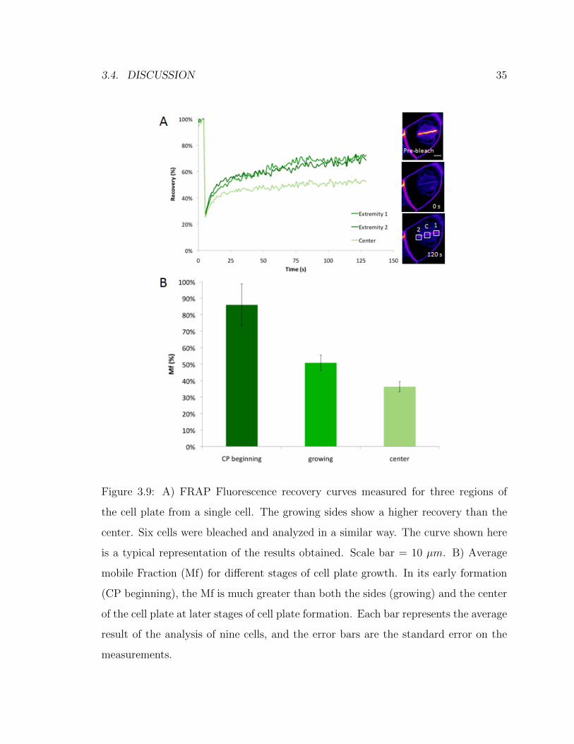
Figure 3.9: A) FRAP Fluorescence recovery curves measured for three regions of

the cell plate from a single cell. The growing sides show a higher recovery than the

center. Six cells were bleached and analyzed in a similar way. The curve shown here

is a typical representation of the results obtained. Scale bar = 10 µm. B) Average

mobile Fraction (Mf) for different stages of cell plate growth. In its early formation

(CP beginning), the Mf is much greater than both the sides (growing) and the center

of the cell plate at later stages of cell plate formation. Each bar represents the average

result of the analysis of nine cells, and the error bars are the standard error on the

measurements.

Chapter 4

Extension of STICS to 3 Dimensions

The STICS technique for 2D and time measurement was introduced in Chapter 2 and

applied to study secretory vesicle transport in BY-2 plant cells undergoing cytokinesis

in Chapter 3, and has been used to study dynamics in a variety of biological systems

since it was first developed [11] [12] [13]. It has been shown to be a robust and

reliable technique, given sufficient spatial and time sampling. However, STICS has

one important limitation: it is restricted to the study of dynamics in a two dimensional

plane set by the spatial resolution of the microscope, whereas the environment of

tissues and non adherent cells is inherently 3D. It is therefore crucial to be able

to study dynamics in three dimensions in order to completely understand biological

processes not restricted to membranes in these cells [34] [35]. Vesicle transport in

dividing plant cells as studied in Chapter 3 also occurs in three dimensions, although

it was only measured here in the 2D focal plane of the cell plate. The work presented

could therefore benefit from an analysis method that can study dynamics in three

dimensions. A few techniques have tried to solve that problem, namely 3D Single

Particle Tracking [36], but they are usually limited in terms of low density labeling

for spatial sampling and tracking a small number of molecules at once. STICS, as

was discussed previously, works very well in high density situations and does not

need to individually resolve each protein. An extension of the technique to a third

36

4.1. THEORY 37

spatial dimension, called 3D STICS, was developed to overcome its limitation to two

dimensions.

This chapter will first present the theory behind the development of 3D STICS,

followed by computer simulations performed to map the detection and spatial sam-

pling of the technique for ranges of parameters such as particle density of immobile

and moving populations; total number of images, particle velocity and image spacing

in the third spatial dimension.

4.1 Theory

The central idea behind 3D STICS is to extend calculation of the spatio-temporal

correlation function to times series of 3D image stacks. A 3D stack is composed of

many 2D (x and y) images separated by a constant spacing in the third (z) spatial

dimension. The z voxel (volume element in 3D) resolution is set by the spacing, in

µm, between each 2D image in z. A schematic representation of a 3D image time

series is shown in Figure 4.1.

Figure 4.1: Schematic representation of a 3D image time series, with k images in the

third spatial dimension, z, and n images in time.

The spatial resolution in x, y and z is set by the 3D PSF of the microscope. Each

2D image from a fluorescence microscope is the integrated intensity distribution from

the spatial convolution of the PSF with the location of all fluorescent point-emitters.

38 CHAPTER 4. EXTENSION OF STICS TO 3 DIMENSIONS

The degree of spreading in space of this PSF reflects on the quality of the optical

system. It is important to note that in the z optical axis, the PSF has a larger

spreading in space than in the other two dimensions for standard objective lenses.

Furthermore, even though 3D STICS calculations approximates the 3D PSF profile

as Gaussian, this is not really the case: the PSF deviates from Gaussian in z. The

spatial resolution is therefore lower in z than it is in x and y [37] [38].

In Chapter 2, we defined in Equation 2.1 a generalized fluorescence intensity fluc-

tuation correlation function for the two spatial lag variables ξ and η and one time lag

variable τ . This function can be extended to three dimensions in space by adding a

third spatial lag variable χ. The equation becomes

rab(ξ, η, χ, τ) =〈δia(x, y, z, t)δib(x+ ξ, y + η, z + χ, t+ τ)〉〈ia(x, y, z, t)〉t〈ib(x, y, z, t+ τ)〉t+τ

(4.1)

We can define a discrete approximation to the function similar to Eq. 2.6. In the

third spatial dimension, z, the discretization comes from the voxel spacing in z in the

image stack. In this case, time is a discrete variable with increments ∆T , the time

taken to image each z stack of 2D images. In terms of the discrete time lag variable

s, the correlation function becomes

raa(ξ, η, χ, s) =1

N − s

N−s∑t=1

〈δia(x, y, z, t)δia(x+ ξ, y + η, z + χ, t+ s)〉〈ia〉t〈ia〉t+s

(4.2)

where N is the total number of image stacks in the time series, the spatial lag

variables ξ, η and χ are voxel shifts in x, y and z, and s is the discrete time-lag

representing the number of image stacks separating the two z stacks being correlated.

The real time-lag, ∆T ∼ τ , is the product of the discrete time lag s, the sampling

time per image frame δt and the number of 2D images in a a stack n: ∆T = nsδt.

In practice, similarly to the 2D version of STICS, the correlation functions are

calculated using Fast Fourier Transforms for computational efficiency:

4.1. THEORY 39

r(ξ, η, χ, s)t =FFT−1[FFT (i(x, y, z, t))FFT (i(x+ ξ, y + η, z + χ, t+ s))∗]

〈i(x, y, z, t)〉〈i(x, y, z, t+ s)〉(4.3)

The 3D STICS algorithm begins by calculating the time lag 0 autocorrelation

function for each image stack in the 3D image time series. Then, for every increment

of the time lag s, the average correlation function of pairs of image stacks in the series

is calculated. For each time lag, the result is a 3D correlation function that can be

fitted to a 3D Gaussian of the form:

r′(ξ, η, χ, s) = g(x(s), y(s), z(s), s) exp(−((ξ − x(s))2 + (η − y(s))2

ω20x,y

+(χ− z(s))2

ω20z

))+g∞(s)

(4.4)

where g(x(s), y(s), z(s), s) is the peak intensity, x(s), y(s) and z(s) are the x, y

and z coordinates of the peak position, ω0x,y is the e−2 waist radius in the x and y

axes, ω0z is the e−2 waist radius in the z axis and g∞ is the long spatial lag offset of

the correlation function. It is important to note that the value of ω0z is greater than

ω0x,y . As discussed previously, the 3D PSF has a larger spreading in z than in the

other dimensions. With CLSM’s, it can be greater than two times the value of ω0x,y

depending on whether the objective lens is overfilled [38].

As in the 2D version of STICS, following the evolution of the fit values as a function

of time lag reveals information about the dynamics of the fluorescent population. If

the fluorescent population under study is undergoing directed flow, the correlation

peak will shift in x, y and z according to its magnitude and direction if the dynamics

are sampled appropriately.

40 CHAPTER 4. EXTENSION OF STICS TO 3 DIMENSIONS

4.2 Computer Simulations

4.2.1 3D simulator

Computer simulations with set inputs were employed to test the collection parameter

space of 3D STICS to investigate the feasibility of the approach. In order to do

this, an existing simulator limited to simulating 2D image time series, programmed

in MatLab by David Kolin of the Wiseman group, was extended to simulate three

dimensional image time series. This 2D simulator worked in the following way: using

a set input density supplied by the user, point particles are given random positions

inside a 2D matrix. The convolution of this matrix with a 2D Gaussian of set e−2

spatial radius is then performed to model the integration of fluorescence from a PSF

with Gaussian profile. Particle positions are recalculated for every image in the time

series, by moving each frame according to the dynamics set by the user input diffusion

coefficient and velocity [39].

The same basic principles apply to the 3D simulator that was developed. Using

the set input density (in particles/µm3) supplied by the user, point particles are

given random positions inside a 3D matrix. The convolution of this matrix with a

3D Gaussian of set e−2 spatial radius in the x and y axes and a larger e−2 spatial

radius in the z axis is performed to model the integration of fluorescence from a 3D

PSF with asymmetric Gaussian intensity profile. The equation for the convolution is

C3D = P3D ∗G3D, where C3D is the resulting 3D convolved matrix, PM is the 3D

particle position matrix and G3D is the 3D Gaussian matrix defined as

G3D = exp (−(2(x− x0)2

ω20x

+2(y − y0)2

ω20y

+2(z − z0)2

ω20z

)) (4.5)

Particle positions are recalculated for every 2D image in the time series, by moving

each frame according to the dynamics set by the user input diffusion coefficient and

velocity in the following way:

4.2. COMPUTER SIMULATIONS 41

x′ = x+ vxδt+ arand√

2Dxδt/px (4.6)

where x’ is the new particle position, x is the previous particle position, δt is the set

sampling time per image frame, vx is the set magnitude of the velocity in the x axis,

arand is a random number taken from a normal distribution with mean 0 and variance

1, Dx is the set diffusion coefficient in the x axis and px is the set voxel resolution

in the x axis. Similar equations hold for the y and z axes. Recalculating particle

positions for every 2D image models the fact that during real microscopy acquisition,

particles in a sample will have moved in the time taken to record one image, although

this does not model faster dynamics on the image frame time scale. Furthermore,

to create a z stack, each 2D image is set to sample the convolved matrix at the

appropriate value of the stack in the z dimension, effectively modeling the focal plane

of a CLSM moving in the z axis during acquisition of 3D-time data. The adjustable

parameters for 3D simulations are shown in Table 4.1. The default values represent

the typical values used for simulations, unless specified otherwise. The PSF size in

the z dimension was taken to be twice as large as the PSF in the x and y dimensions

to model the 3D PSF of a CLSM. Values of pixel size and sampling time used are

also typical of confocal laser-scanning microscopy. Most simulations presented in this

chapter are done with velocity components in the x and y dimensions set to 0 and

set to 0.01 µm/s in the z dimension, in order to characterize the capabilities of the

technique in this new dimension.

To give a general idea of the size and shape of the correlation function in the three

spatial dimensions, contour plots of correlation functions calculated from computer

simulations are presented in Figures 4.2 and 4.3. Both simulations were performed

with a PSF size of 0.4 µm in x and y and of 0.8 µm in z. Figure 4.2 shows contour

plots in the x-y (A) and x-z (B) planes of the autocorrelation function of a 3D stack of

64 images in z of 64x64 pixels, with a pixel size of 0.1 µm and a z spacing of 0.1 µm.

The effect on the 3D correlation function of the larger PSF size in the z dimension

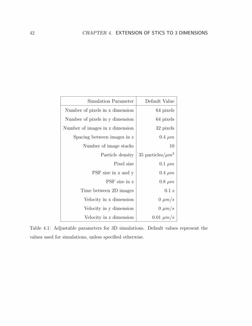
42 CHAPTER 4. EXTENSION OF STICS TO 3 DIMENSIONS

Simulation Parameter Default Value

Number of pixels in x dimension 64 pixels

Number of pixels in y dimension 64 pixels

Number of images in z dimension 32 pixels

Spacing between images in z 0.4 µm

Number of image stacks 10

Particle density 35 particles/µm3

Pixel size 0.1 µm

PSF size in x and y 0.4 µm

PSF size in z 0.8 µm

Time between 2D images 0.1 s

Velocity in x dimension 0 µm/s

Velocity in y dimension 0 µm/s

Velocity in z dimension 0.01 µm/s

Table 4.1: Adjustable parameters for 3D simulations. Default values represent the

values used for simulations, unless specified otherwise.

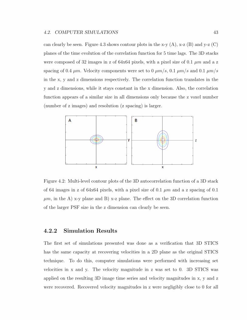
4.2. COMPUTER SIMULATIONS 43

can clearly be seen. Figure 4.3 shows contour plots in the x-y (A), x-z (B) and y-z (C)

planes of the time evolution of the correlation function for 5 time lags. The 3D stacks

were composed of 32 images in z of 64x64 pixels, with a pixel size of 0.1 µm and a z

spacing of 0.4 µm. Velocity components were set to 0 µm/s, 0.1 µm/s and 0.1 µm/s

in the x, y and z dimensions respectively. The correlation function translates in the

y and z dimensions, while it stays constant in the x dimension. Also, the correlation

function appears of a similar size in all dimensions only because the z voxel number

(number of z images) and resolution (z spacing) is larger.

Figure 4.2: Multi-level contour plots of the 3D autocorrelation function of a 3D stack

of 64 images in z of 64x64 pixels, with a pixel size of 0.1 µm and a z spacing of 0.1

µm, in the A) x-y plane and B) x-z plane. The effect on the 3D correlation function

of the larger PSF size in the z dimension can clearly be seen.

4.2.2 Simulation Results

The first set of simulations presented was done as a verification that 3D STICS

has the same capacity at recovering velocities in a 2D plane as the original STICS

technique. To do this, computer simulations were performed with increasing set

velocities in x and y. The velocity magnitude in z was set to 0. 3D STICS was

applied on the resulting 3D image time series and velocity magnitudes in x, y and z

were recovered. Recovered velocity magnitudes in z were negligibly close to 0 for all

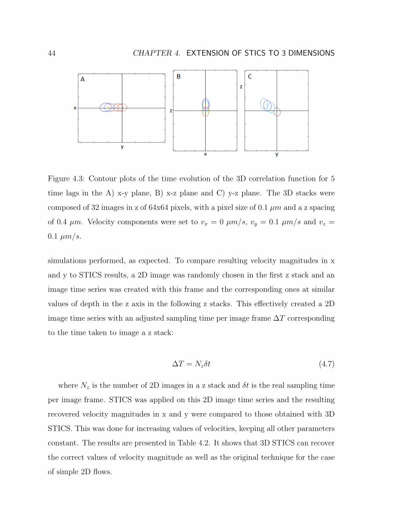
44 CHAPTER 4. EXTENSION OF STICS TO 3 DIMENSIONS

Figure 4.3: Contour plots of the time evolution of the 3D correlation function for 5

time lags in the A) x-y plane, B) x-z plane and C) y-z plane. The 3D stacks were

composed of 32 images in z of 64x64 pixels, with a pixel size of 0.1 µm and a z spacing

of 0.4 µm. Velocity components were set to vx = 0 µm/s, vy = 0.1 µm/s and vz =

0.1 µm/s.

simulations performed, as expected. To compare resulting velocity magnitudes in x

and y to STICS results, a 2D image was randomly chosen in the first z stack and an

image time series was created with this frame and the corresponding ones at similar

values of depth in the z axis in the following z stacks. This effectively created a 2D

image time series with an adjusted sampling time per image frame ∆T corresponding

to the time taken to image a z stack:

∆T = Nzδt (4.7)

where Nz is the number of 2D images in a z stack and δt is the real sampling time

per image frame. STICS was applied on this 2D image time series and the resulting

recovered velocity magnitudes in x and y were compared to those obtained with 3D

STICS. This was done for increasing values of velocities, keeping all other parameters

constant. The results are presented in Table 4.2. It shows that 3D STICS can recover

the correct values of velocity magnitude as well as the original technique for the case

of simple 2D flows.

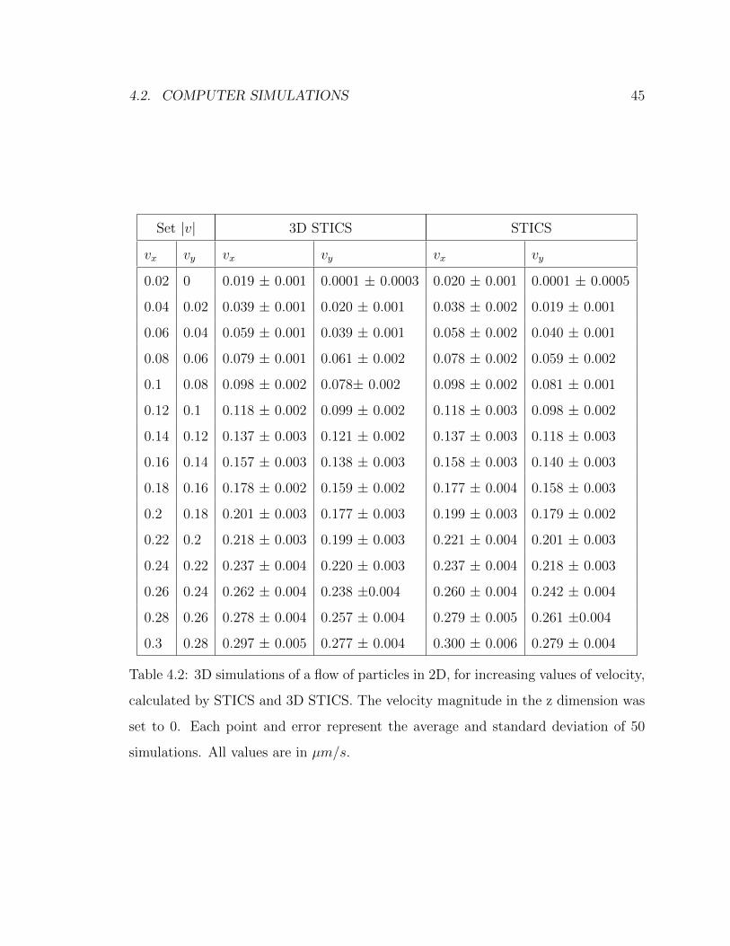
4.2. COMPUTER SIMULATIONS 45

Set |v| 3D STICS STICS

vx vy vx vy vx vy

0.02 0 0.019 ± 0.001 0.0001 ± 0.0003 0.020 ± 0.001 0.0001 ± 0.0005

0.04 0.02 0.039 ± 0.001 0.020 ± 0.001 0.038 ± 0.002 0.019 ± 0.001

0.06 0.04 0.059 ± 0.001 0.039 ± 0.001 0.058 ± 0.002 0.040 ± 0.001

0.08 0.06 0.079 ± 0.001 0.061 ± 0.002 0.078 ± 0.002 0.059 ± 0.002

0.1 0.08 0.098 ± 0.002 0.078± 0.002 0.098 ± 0.002 0.081 ± 0.001

0.12 0.1 0.118 ± 0.002 0.099 ± 0.002 0.118 ± 0.003 0.098 ± 0.002

0.14 0.12 0.137 ± 0.003 0.121 ± 0.002 0.137 ± 0.003 0.118 ± 0.003

0.16 0.14 0.157 ± 0.003 0.138 ± 0.003 0.158 ± 0.003 0.140 ± 0.003

0.18 0.16 0.178 ± 0.002 0.159 ± 0.002 0.177 ± 0.004 0.158 ± 0.003

0.2 0.18 0.201 ± 0.003 0.177 ± 0.003 0.199 ± 0.003 0.179 ± 0.002

0.22 0.2 0.218 ± 0.003 0.199 ± 0.003 0.221 ± 0.004 0.201 ± 0.003

0.24 0.22 0.237 ± 0.004 0.220 ± 0.003 0.237 ± 0.004 0.218 ± 0.003

0.26 0.24 0.262 ± 0.004 0.238 ±0.004 0.260 ± 0.004 0.242 ± 0.004

0.28 0.26 0.278 ± 0.004 0.257 ± 0.004 0.279 ± 0.005 0.261 ±0.004

0.3 0.28 0.297 ± 0.005 0.277 ± 0.004 0.300 ± 0.006 0.279 ± 0.004

Table 4.2: 3D simulations of a flow of particles in 2D, for increasing values of velocity,

calculated by STICS and 3D STICS. The velocity magnitude in the z dimension was

set to 0. Each point and error represent the average and standard deviation of 50

simulations. All values are in µm/s.

46 CHAPTER 4. EXTENSION OF STICS TO 3 DIMENSIONS

The second set of simulations was done to verify that 3D STICS achieves its goal of

recovering velocities in the third spatial dimension and to test the range of velocities

at which it obtains precise and accurate results. Setting velocity magnitudes in x and

y to 0, 3D STICS was applied on simulations of flowing populations with increasing

values of velocities in the z dimension, keeping all other parameters constant. The

results are shown in Figure 4.4.

Figure 4.4: 3D STICS results for computer simulations with increasing values of ve-

locity magnitudes in the z dimension. Velocity magnitudes in the x and y dimensions

were set to 0. Each point and error bars represent the average and standard deviation

of 50 simulations.

As can be seen, the technique performs rather well for smaller values of velocities,

but results start to deviate at higher values of velocities. This is because as the

velocity magnitude increases, the displacement of particles in the z dimension within

a z stack in the time taken to image it becomes non negligible. With the parameters

4.2. COMPUTER SIMULATIONS 47

used for the simulations shown in Table 4.1, an image stack takes 3.2 seconds to

image. At a velocity of 0.5 µm/s, the particles move 1.6 µm in the time it takes to

image a single stack. As the correlation function is calculated from such an image

time series, it will be more spread out in the axis of movement. Figure 4.5 shows the

autocorrelation function of a 3D stack composed of 32 images of 64x64 pixels, with a

pixel size of 0.1 µm and a z spacing of 0.4 µm, without flow (A) and with a flow in the

z direction of 0.5 µm/s (B). The spreading of the correlation function is due to the

movement of particles. For higher time lags, the correlation function in Figure 4.5B

will quickly move past the edge of the correlation window, at which point part of it

will reappear on the other side. The fit values of such a correlation function to a 3D

Gaussian will be incorrectly calculated, resulting in an incorrect peak position. This

effect is lessened as the imaging rate is increased. Current high-speed microscopes,

which can record hundreds of images in a second, will not be as affected by this error,

although there will always be a sampling limit.

Figure 4.5: Spatial spreading of the correlation function. A) x-z plane of the autocor-

relation function of a 3D stack composed of 32 images of 64x64 pixels, with a pixel

size of 0.1 µm and a z spacing of 0.4 µm, without flow. B) x-z plane of the autocor-

relation function of a similar 3D stack with particles flowing in the z dimension at a

rate of 0.5 µm/s. The spreading of the correlation function is due to the movement

of particles.

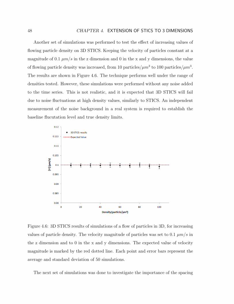
48 CHAPTER 4. EXTENSION OF STICS TO 3 DIMENSIONS

Another set of simulations was performed to test the effect of increasing values of

flowing particle density on 3D STICS. Keeping the velocity of particles constant at a

magnitude of 0.1 µm/s in the z dimension and 0 in the x and y dimensions, the value

of flowing particle density was increased, from 10 particles/µm3 to 100 particles/µm3.

The results are shown in Figure 4.6. The technique performs well under the range of

densities tested. However, these simulations were performed without any noise added

to the time series. This is not realistic, and it is expected that 3D STICS will fail

due to noise fluctuations at high density values, similarly to STICS. An independent

measurement of the noise background in a real system is required to establish the

baseline flucutation level and true density limits.

Figure 4.6: 3D STICS results of simulations of a flow of particles in 3D, for increasing

values of particle density. The velocity magnitude of particles was set to 0.1 µm/s in

the z dimension and to 0 in the x and y dimensions. The expected value of velocity

magnitude is marked by the red dotted line. Each point and error bars represent the

average and standard deviation of 50 simulations.

The next set of simulations was done to investigate the importance of the spacing

4.2. COMPUTER SIMULATIONS 49

between images in a 3D stack and the number of images used to create the z stacks.

With the original version of STICS, a criterion for accurate and precise results was

sufficient spatial resolution and sampling. There is a lower limit on the sampling

required in order to have enough averaging of the correlation function to obtain

reliable and meaningful results. It was found that the smallest usable region of interest

(ROI) for ICS and STICS analysis was a region of 16x16 pixels2 area for typical

imaging with a high NA objective lens [14]. A similar condition should exist on

the sampling required in the z dimension. Also, as was discussed in Chapter 2,

it is important for spatial correlation for the signal from each point-source to be

oversampled: the spatial convolution of the PSF with the location of all fluorescent

point-emitters causes the integrated emission to be spread over a number of adjacent

pixels in the image, to an extent dependent on the size of the PSF and the pixel

size. The same principle applies to 3D STICS for the third spatial dimension. To get

oversampling in the z dimension, it is important to image 3D stacks with a z spacing

smaller than the diameter of the PSF in z.

Keeping the velocity of particles constant at a magnitude of 0.1 µm/s in the z

dimension and 0 in the x and y dimensions, the z spacing was varied from 0.2 µm to

2 µm and tested for z stacks of 16, 32 and 48 images. The results are summarized in

Table 4.3, where ∆z is the z spacing between images in µm and ∆N z is the number of

images in a z stack. Each value shown is the average of the results of 50 simulations

and the error is the standard deviation on these results. These show that 3D STICS

fails to be accurate for large z spacing, as expected, because the signal from each

point-source is not oversampled enough in z. The technique also has lower accuracy

for z stacks of 16 images because there is less averaging of the correlation function at

that size: half the number of fluctuations are expected to be sampled compared to z

stacks of 32 images.

To illustrate the effect of sampling in three spatial dimensions and how it is dif-

ferent in z because of the larger PSF size, simulations of particles flowing with equal

50 CHAPTER 4. EXTENSION OF STICS TO 3 DIMENSIONS

HHHHHHH

HH∆z

∆N z16 32 48

0.2 0.083±0.004 0.098±0.002 0.102±0.001

0.4 0.092±0.003 0.099±0.001 0.1016±0.0006

0.6 0.100±0.004 0.100±0.001 0.1001±0.0009

0.8 0.102±0.004 0.098±0.001 0.1017±0.0005

1.0 0.095±0.006 0.102±0.002 0.0996±0.0009

1.2 0.10±0.01 0.09±0.01 0.104±0.005

1.4 0.10±0.02 0.09±0.01 0.108±0.008

1.6 0.12±0.03 0.091±0.008 0.08± 0.01

1.8 0.12±0.03 0.094±0.006 0.08±0.01

2.0 0.14±0.04 0.096±0.004 0.09±0.01

Table 4.3: 3D STICS simulation analysis results for the measured z-velocity (set value

vz = 0.1 µm/s). ∆z is the spacing between images in µm and ∆N z is the number

of images in a stack. The velocity magnitude of particles was set at 0 in the x and y

dimensions. Each value and error represent the average and standard deviation of 50

simulations.

4.2. COMPUTER SIMULATIONS 51

velocity components in all three dimensions were performed. The velocity of flow-

ing particles was increased from vx = vy = vz = 0.05 µm/s to vx = vy = vz = 0.5

µm/s, in 3D stacks of 32 images, 32x32 pixels, with a pixel size of 0.4 µm and a z

spacing of 0.4 µm. The only difference in the resulting recovered velocity components

should therefore come from the difference in sampling in z compared to x and y. The

principle behind STICS and 3D STICS is to sample fluctuations in space and time,

with the PSF acting as the correlator. In 2D, the sampling of spatial fluctuations

depends on how many beam areas are sampled per ROI. In 3D, the number of PSF

fluctuation volumes sampled will depend on the direction, since it is the PSF is lager

in z. However, there will also be a temporal component: the particles will not cross

the PSF as fast in z as in x and y. The results presented in Figure 4.7 clearly show

the effect of the larger PSF size in z. For smaller velocity values, 3D STICS can

recover the set velocity component in z as well as in x and y, indicating that the lower

sampling in z is compensated by the fact that particles take more time to cross the

PSF in that direction. However, for higher velocity values, this effect is lessened by

the fast flow of the particles, and recovered velocity components in z start to deviate

due to lower sampling. Each point and error bars in the figure represent the average

and standard deviation of 50 simulations.

The final set of simulations performed was done to investigate velocity recovery in

the presence of an immobile population. As mentioned in Chapter 2, there will often

be immobile or slow-moving populations present that can represent an important

fraction of the total fluorescence signal. This population will correlate strongly in

space and time and, for small time lags, can mask the smaller correlation peak of a

translating population in the vicinity of zero spatial lags, making it difficult to track

the correlation function’s peak location in order to calculate velocities. Therefore, a

filter is needed to remove the contribution of the immobile population. In this 3D

case, this can be done in a similar way as with STICS, by removing the DC component

of each pixel’s time trace by filtering in Fourier space. The corrected pixel intensities

52 CHAPTER 4. EXTENSION OF STICS TO 3 DIMENSIONS

Figure 4.7: 3D STICS results of simulations with increasing and equal velocity com-

ponents in all three spatial dimensions in 3D stacks of 32 images, 32x32 pixels, with

a pixel size of 0.4 µm and a z spacing of 0.4 µm. The effect of the larger PSF size

in z (0.8 µm compared to 0.4 µm) can clearly be seen. Each point and error bars

represent the average and standard deviation of 50 simulations.

are given by:

i′(x, y, z, t) = F−1f Ft(i(x, y, z, t))×H 1T

(f) (4.8)

where T is the total time of the series, F−1f is the inverse Fourier transform with

respect to frequency, Ft is the Fourier transform with respect to time, and H 1T

(f) is

the Heaviside function which is zero for f < 1/T and one for f ≥ 1/T .

The results shown in Figure 4.8 present the velocities recovered by 3D STICS for

simulated image time series containing an immobile population of increasing density

and a flowing population of set constant density. The immobile population density

was increased from 10 particles/µm3 to 100 particles/µm3. The velocity of the moving

4.2. COMPUTER SIMULATIONS 53

particles was set at a constant magnitude of 0.1 µm/s in the z dimension and 0 in

the x and y dimensions. The density of the flowing population is kept constant at

a value of 35 particles/µm3. Once the image series is filtered, 3D STICS is able to

recover the flowing population’s velocity, with no significant change even when 75%

of the total population is immobile.

Figure 4.8: 3D STICS results of simulations with flowing and filtered immobile pop-

ulations, for increasing values of immobile population particle density. The velocity

magnitude of flowing particles was kept at a constant value of 0.1 µm/s in the z di-

mension and at a value of 0 in the x and y dimensions. The expected value of velocity

magnitude is marked by the red dotted line. Each point and error bars represent the

average and standard deviation of 50 simulations.

From the computer simulations shown above, it is clear that 3D STICS performs

well under parameters consistent with current CLSM microscopes. Results could even

be improved by using faster imaging systems such as spinning-disk microscopes, ca-

pable of imaging hundreds of images in a second. However, faster imaging rates can

result in significant photobleaching, which could be incorporated into future simula-

54 CHAPTER 4. EXTENSION OF STICS TO 3 DIMENSIONS

tions. 3D STICS was only tested so far with computer-simulated image time series.

Before the technique can be applied in real studies, it will have to be tested with

real control experiments and the results obtained compared to those of an estab-

lished technique, like 3D single particle tracking at labeling densities accessible to

both. There is a great number of potential avenues to be explored with 3D STICS.

Other biological processes that were previously studied with STICS could be ideal

test subjects for the new 3D version of the technique, such as vesicle transport and

delivery dynamics in dividing plant cells. Intracellular endosomal delivery and traf-

ficking would be another candidate system for this method. Although some details

of 3D STICS remain to be explored, the work presented in this chapter represents

a stepping stone in the development of a new 3D correlation technique. With this

powerful tool, more biologically relevant and complex systems will be accessible and

perhaps reveal new details on molecular transport mechanisms that are essential to

cell function.

Chapter 5

Conclusion

New applications developments to the spatio-temporal image correlation spectroscopy

(STICS) technique were presented in this thesis. Chapter 3 illustrated its application

for measurements of secretory vesicle dynamics carrying new cell wall material inside

dividing tobacco BY-2 cells. Due to their small size and high density, quantitative

information on the dynamics of these vesicles had always been difficult to obtain.

The STICS technique was successful in measuring velocity maps for the secretory

vesicles from fluorescence microscopy image time series. The values of the velocity

flow obtained varied depending on the stage of cell division. In parallel, the growth

rate of the cell plate was measured using fluorescence morphological operators soft-

ware (FluMOS). It was discovered that the cell plate passed through three specific

phases: an accumulation of vesicles at the site of fusion, followed by a period of high

growth rate until the cell plate reached an approximate diameter of 15 µm, and fi-

nally another slower period of growth until the cell plate reached and attached to

the parental plasma membrane. These stages match well with the dynamics of the

vesicles that were characterized using STICS: slow velocities as the vesicles accumu-

late at the center, rapid and active trafficking as the cell plate first starts expanding,

and slower dynamics focused on the growing extremities as it finishes its matura-

tion. This study sheds new light on the rate of vesicle transport to the cell plate and

55

56 CHAPTER 5. CONCLUSION

how it evolves throughout cell plate formation. Previous studies have used electron

tomography [23], drugs, inhibitors [30], beads and synthetic vesicles to study this

process [32], but none combined live imaging of dividing plant cells and analysis of

the dynamics of endogenous fluorescent secretory vesicles. This work represents the

first comprehensive characterization of secretory vesicle dynamics during plant cell

cytokinesis.

Chapter 4 presented the extension of STICS to three spatial dimensions. Although

the original STICS technique has proven useful for a number of membrane biophysics

applications, it is restricted to the study of dynamics in two dimensions, which is

not always biologically relevant. To overcome this restriction, an extension of the

technique to a third spatial dimension was developed. Its capabilities and limits

were extensively tested using computer simulations. The new technique was first

compared to its 2D predecessor by testing its ability to calculate velocities in a 2D

plane. Then, its efficacy at recovering velocities in the third spatial dimension was

tested. The effects of the densities of the immobile and moving population, as well as

the number of images and resolution in the third spatial dimension was investigated.

The simulations done in this chapter revealed that the technique performs well under

parameters easily achieved with current high-speed microscopes. However, before

it can be applied to study biological systems, the technique remains to be tested

on controlled experimental data and compared with the results of an established

technique such as 3D single particle tracking.

There is a great number of potential avenues to be explored with 3D STICS. One of

them ties in with Chapter 3 of this thesis: the technique could be used to study vesicle

dynamics in three dimensions in plant cells. Vesicles and other organelles do of course

have three degrees of translational freedom in the three dimensional space of the cell.

Therefore, in order to obtain a more complete picture of intracellular trafficking, the

acquisition of 3D image time series would be needed in adherent cell tissue culture.

Other biological systems that were previously studied with STICS could be ideal

57

test subjects for the new 3D version of the technique, such as a study of adhesion

complexes in cells migrating inside a 3D matrix, which is closer to the tissue context

for cell migration [34] [35]. Although some details of 3D STICS remain to be explored,

the work presented in this thesis represents a stepping stone in the development of a

new 3D correlation technique. With this new powerful tool, more biologically relevant

and complex systems will be accessible to researchers and perhaps reveal new details

on molecular transport mechanisms that are essential to cell function.

Bibliography

[1] O. Shimomura, F. Johnson, and Y. Saiga, “Extraction, purification and prop-erties of aequorin, a bioluminescent protein from the luminous hydromedusan,aequorea,” J. Cell. Comp. Physiol., vol. 59, 1962.

[2] B. Valeur, Molecular Fluorescence: Principles and Applications. Wiley, 2002.

[3] A. Jablonski, “ber den Mechanismus der Photolumineszenz von Farbstoffphos-phoren,” Zeitschrift Fr Physik, vol. 94, pp. 38–46, 1935.

[4] M. Monsky, “Memoirs on inventing the confocal scanning microscope,” Scanning,vol. 10(4), pp. 128–138, 1988.

[5] B. Hebert, Spatio-temporal Image Correlation Spectroscopy: Development andImplementation in Living Cells. PhD thesis, Physics Department, McGill Uni-versity, 2006.

[6] S. Paddock, “Confocal laser scanning microscopy,” BioTechniques, vol. 27,pp. 992–1004, 1999.

[7] D. Magde, E. Elson, and W. W. Webb, “Thermodynamic fluctuations in a re-acting system: measurement by fluorescence correlation spectroscopy,” PhysicalReview Letters, vol. 29(11), pp. 705–708, 1972.

[8] E. Haustein and P. Schwille, “Fluorescence correlation spectroscopy: novel vari-ation of an established technique,” Annu Rev Biophys Biomol Struct, vol. 36,pp. 151–169, 2007.

[9] N. Petersen, P. Hddelius, P. W. Wiseman, O. Seger, and K.-E. Magnusson,“Quatitation of membrane receptor distributions by image correlation spec-troscopy: concept and application,” Biophysical Journal, vol. 65, pp. 1135–1146,1993.

[10] P. W. Wiseman and N. O. Petersen, “Image correlation spectroscopy: optimiza-tion for ultrasensitive detection of preexisting platelet-derived growth factor-betareceptor oligomers on intact cells,” Biophysical Journal, vol. 76(2), pp. 963–977,1999.

58

BIBLIOGRAPHY 59

[11] B. Hebert, S. Constantino, and P. W. Wiseman, “Spatiotemporal image cor-relation spectroscopy (STICS) theory, verification, and application to proteinvelocity mapping in living CHO cells,” Biophysical Journal, vol. 88, pp. 3601–3614, 2005.

[12] C. Brown, B. Hebert, D. Kolin, J. Zareno, A. Horwitz, and P. W. Wiseman,“Probing the integrin-actin linkage using high-resolution protein velocity map-ping,” Journal of Cell Science, vol. 119, pp. 5204–5214, 2006.

[13] J. Bove, B. Vaillancourt, J. Kroeger, P. K. Hepler, P. W. Wiseman, and A. Geit-mann, “Magnitude and direction of vesicle dynamics in growing pollen tubesusing spatiotemporal image correlation spectroscopy (STICS) and fluorescencerecovery after photobleaching (FRAP),” Plant Physiology, vol. 147(4), pp. 1646–1658, 2008.

[14] S. Constantino, J. Comean, D. Kolin, and P. W. Wiseman, “Accuracy and dy-namic range of spatial image correlation spectroscopy and cross-correlation spec-troscopy,” Biophysical Journal, vol. 89, pp. 1251–1260, 2005.

[15] G. M. Cooper and R. E. Hausman, The Cell: a molecular approach (5th Edition).Sinauer Associates Inc., 2009.

[16] D. Verma, “Cytokinesis and building of the cell plate in plants,” Annu Rev PlantPhysiol Plant Mol Biol, vol. 52, pp. 751–784, 2001.

[17] T. M. Molchan, A. H. Valster, and P. K. Hepler, “Actomyosin promotes cellplate alignment and late lateral expansion in Tradescantia stamen hair cells,” JCell Biol, vol. 130, pp. 1345–1357, 1995.

[18] A. L. Samuels, T. H. J. Giddings, and S. L. A., “Cytokinesis in tobacco BY-2and root tip cells: a new model of cell plate formation in higher plants,” Planta,vol. 214(5), pp. 683–693, 2002.

[19] M. S. Otegui and S. L. A., “Electron tomographic analysis of post-meiotic cytoki-nesis during pollen development in Arabidopsis thaliana,” Planta, vol. 218(4),pp. 501–515, 2004.

[20] J. M. Seguı-Simarro, J. R. Austin, E. A. White, and L. A. Staehelin, “Electrontomographic analysis of post-meiotic cytokinesis during pollen development inArabidopsis thaliana,” Plant Cell, vol. 16, pp. 836–856, 2004.

[21] J. M. Seguı-Simarro and L. A. Staehelin, “Cell cycle-dependent changes in Golgistacks, vacuoles, clathrin-coated vesicles and multivesicular bodies in meristem-atic cells of Arabidopsis thaliana: quantitative and spatial analysis,” Planta,vol. 223, pp. 223–236, 2006.

[22] A. Nebenfur, “Organelle dynamics during cell division,” Plant Cell Monogr,vol. 9, pp. 195–206, 2007.

60 BIBLIOGRAPHY

[23] M. S. Seguı-Simarro, Otegui, J. M., J. R. Austin, and L. A. Staehelin, “Electrontomographic analysis of post-meiotic cytokinesis during pollen development inArabidopsis thaliana,” Plant Cell Monogr, vol. 9, pp. 251–287, 2008.

[24] K. Ueda, S. Sakaguchi, F. Kumagai, S. Hasezawa, H. Quader, and U. Kristen,“Development and disintegration of phragmoplasts in living cultured cells ofa GFP::TUA6 transgenic Arabidopsis thaliana plant,” Protoplasma, vol. 220,pp. 111–118, 2003.

[25] T. Nagata and F. Kumagai, “Plant cell biology through the window of the highlysynchronized tobacco BY-2 cell line,” Methods Cell Sci, vol. 21(2-3), pp. 123–127,1999.

[26] P. Dhonukshe and T. W. J. J. Gadella, “Alteration of microtubule dynamicinstability during preprophase band formation revealed by Yellow FluorescenceProtein-CLIP170 microtubule plus-end labeling,” Plant Cell, vol. 15(3), pp. 597–611, 2003.

[27] M. H. Lauber, I. Waizenegger, T. Steinmann, H. Schwarz, U. Mayer, I. Hwang,W. Lukowitz, and G. Jurgens, “The Arabidopsis KNOLLE protein is acytokinesis-specific syntaxin,” J Cell Biol, vol. 139(6), pp. 1485–1493, 1997.

[28] M. Edidin, Y. Zagyansky, and T. J. Lardner, “Measurement of membrane proteinlateral diffusion in single cells,” Science, vol. 191, pp. 466–468, 1976.

[29] A. J. Reits and J. J. Neefjes, “From fixed to FRAP: measuring protein mobilityand activity in living cells,” Nature Cell Biol, vol. 3, pp. E145–E147, 2001.

[30] T. Higaki, N. Kutsuna, T. Sano, and S. Hasezawa, “Quantitative analysis ofchanges in actin microfilament contribution to cell plate development in plantcytokinesis,” BMC Plant Biol, vol. 8, p. 80, 2008.

[31] N. Kutsuna, F. Kumagai, M. H. Sato, and S. Hasezawa, “Quantitative analysisof changes in actin microfilament contribution to cell plate development in plantcytokinesis,” Plant Cell Physiol, vol. 44(10), pp. 1045–1054, 2003.

[32] A. Esseling-Ozdoba, J. W. Vos, A. A. M. van Lammeren, and A. M. C. Emons,“Synthetic lipid (DOPG) vesicles accumulate in the cell plate region but do notfuse,” Plant Physiol, vol. 147, pp. 1699–1709, 2008.

[33] A. Esseling-Ozdoba, R. A. Kik, A. A. M. van Lammeren, J. M. Kleijn, andE. A. M. C., “Flexibility contra stiffness: the phragmoplast as a physical barrierfor beads but not for vesicles,” Plant Physiol, vol. 152(2), pp. 1065–1072, 2010.

[34] D. J. Webb and A. F. Horwitz, “New dimensions in cell migration,” Nature CellBiol, vol. 5, pp. 690–692, 2003.

BIBLIOGRAPHY 61

[35] T. Jacks and R. A. Weinberg, “Taking the study of cancer cell survival to a newdimension,” Cell, vol. 111, pp. 923–925, 2002.

[36] I. M. Peters, B. G. De Grooth, J. M. Schins, C. G. Figdor, and J. Greve,“Three-dimensional single-particle tracking with nanometer resolution,” Rev SciInstrum, vol. 69, pp. 2762–2766, 1998.

[37] R. W. Cole, T. Jinadasa, and C. M. Brown, “Measuring and interpreting pointspread functions to determine confocal microscope resolution and ensure qualitycontrol,” Nature Protocols, vol. 6, pp. 1929–1941, 2011.

[38] S. T. Hess and W. W. Webb, “Focal volume optics and experimental artifacts inconfocal fluorescence correlation spectrsocopy,” Biophysical Journal, vol. 83(4),pp. 2300–2317, 2002.

[39] D. L. Kolin, k-Space Image Correlation Spectroscopy: Theory, Verification, andApplications. PhD thesis, Department of Chemistry, McGill University, 2008.