Embed Size (px)
Citation preview
ConsumerEquilibriumand Market
Demand
Chapter 4
Discussion Topics
What are the conditions that describe your initial purchase decision?
What makes you change your purchase decision?
A representation of the law of demandWhat is meant by tastes and
preferencesUse of consumer surplus for benefit
calculation2
Measurement andInterpretation of
Consumer Equilibrium(Purchase Decision)
3
Consumer EquilibriumRemember that utility represents the level
of satisfaction obtained from alternative bundles (or collection) of goods
Assume the consumer wants to maximize utility given his/her limited budget We also assume that utility only impacted by
the consumption of market goods (i.e. price exists)
How can we represent this problem graphically and mathematically?
Page 54
Incr
easin
g Util
ity
Page 54
Consumer Equilibrium
Good 1
Good 2
U4
U2
U3
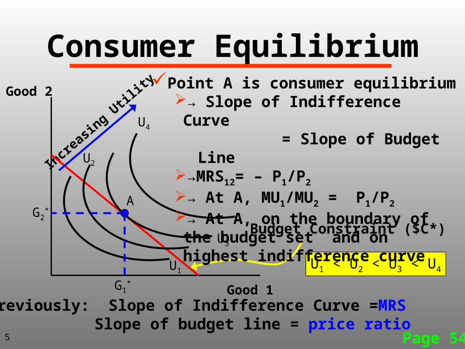
U1U1 < U2 < U3 < U4
Budget Constraint ($C*)
A
G1*
G2*
Point A is consumer equilibrium→ Slope of Indifference Curve
= Slope of Budget Line→MRS12= – P1/P2
→ At A, MU1/MU2 = P1/P2
→ At A, on the boundary of the budget set and on highest indifference curve
Previously: Slope of Indifference Curve =MRS Slope of budget line = price ratio
5
Page 54
Consumer Equilibrium
Good 1
Good 2
U4
U2
U3
U1
A
G1*
G2*
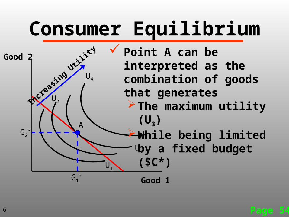
Point A can be interpreted as the combination of goods that generates The maximum utility (U3)While being limited by a
fixed budget ($C*)
Incr
easin
g Util
ity
6
Page 54
Consumer Equilibrium
Good 1
Good 2
U3
A
G1*
G2*
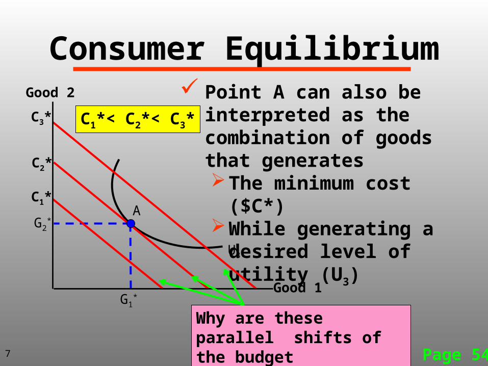
Point A can also be interpreted as the combination of goods that generates The minimum cost ($C*)While generating a desired
level of utility (U3)
Why are these parallel shifts of the budget constraint?
C1*
C2*
C3* C1*< C2*< C3*
7
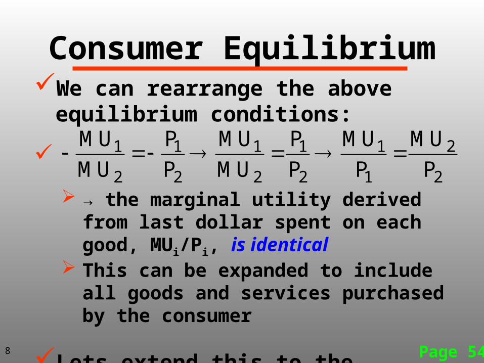
Consumer EquilibriumWe can rearrange the above equilibrium
conditions:
→ the marginal utility derived from last dollar spent on each good, MUi/Pi, is identical
This can be expanded to include all goods and services purchased by the consumer
Lets extend this to the textbook example of tacos vs. hamburger consumption Page 54
1 1 1 1 1 2
2 2 2 2 1 2
MU P MU P MU MU
MU P MU P P P
8
Page 54
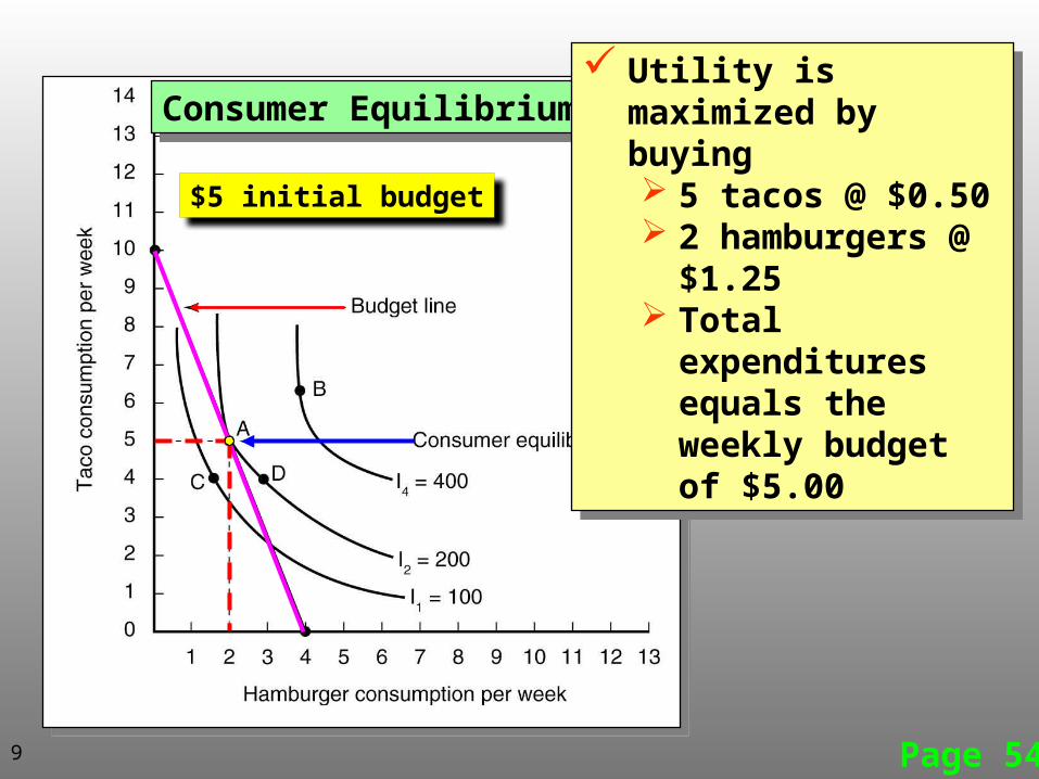
Consumer EquilibriumConsumer Equilibrium Utility is maximized by
buying 5 tacos @ $0.50 2 hamburgers @
$1.25 Total expenditures
equals the weekly budget of $5.00
Utility is maximized by buying 5 tacos @ $0.50 2 hamburgers @
$1.25 Total expenditures
equals the weekly budget of $5.00
9
$5 initial budget
Page 54
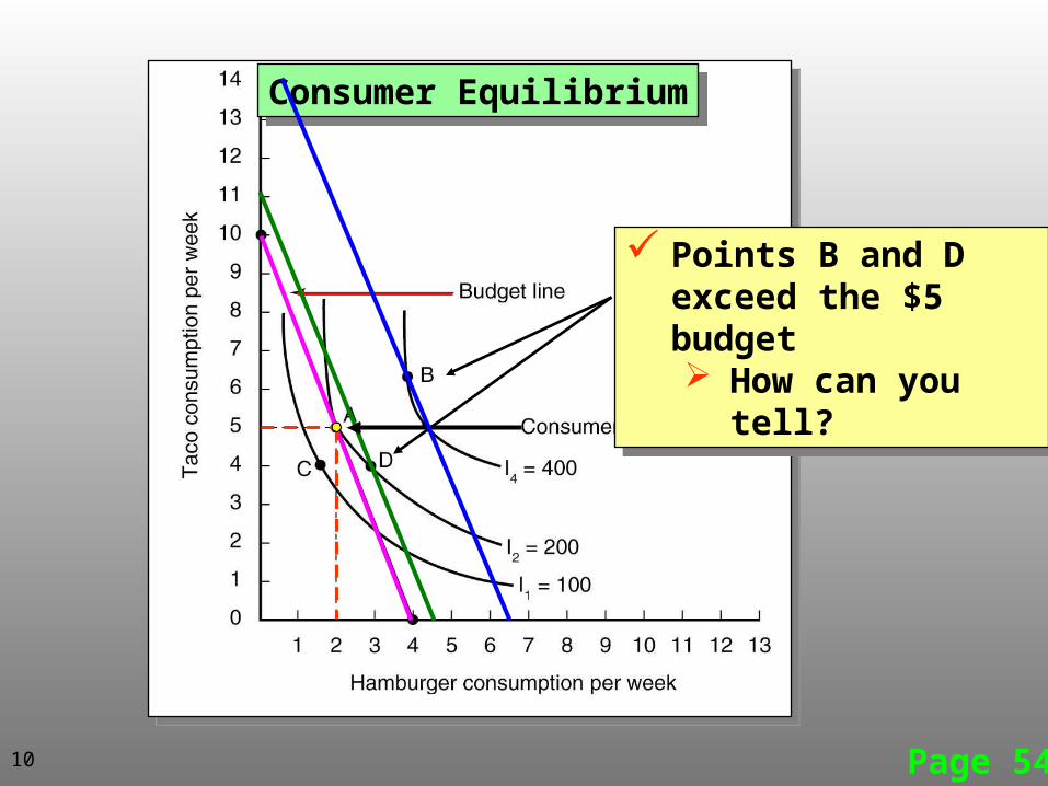
Consumer EquilibriumConsumer Equilibrium
Points B and D exceed the $5 budget How can you tell?
Points B and D exceed the $5 budget How can you tell?
10
Page 54
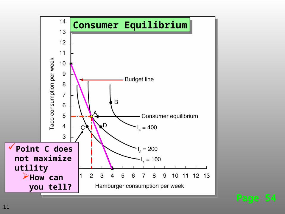
Consumer EquilibriumConsumer Equilibrium
Point C does not maximize utility
How can you tell?
11
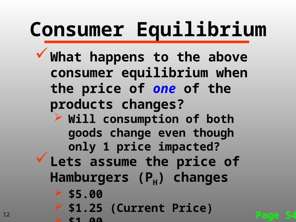
Consumer EquilibriumWhat happens to the above
consumer equilibrium when the price of one of the products changes? Will consumption of both goods
change even though only 1 price impacted?
Lets assume the price of Hamburgers (PH) changes $5.00 $1.25 (Current Price) $1.00
Page 5412
Effect of Price Changes
Page 54
1 2 3 4 5 6
1
3
2
4
5
6
7
8
9
10
11
D
Hamburger Consumption per Week
Tac
o C
onsu
mpt
ion
per
Wee
k
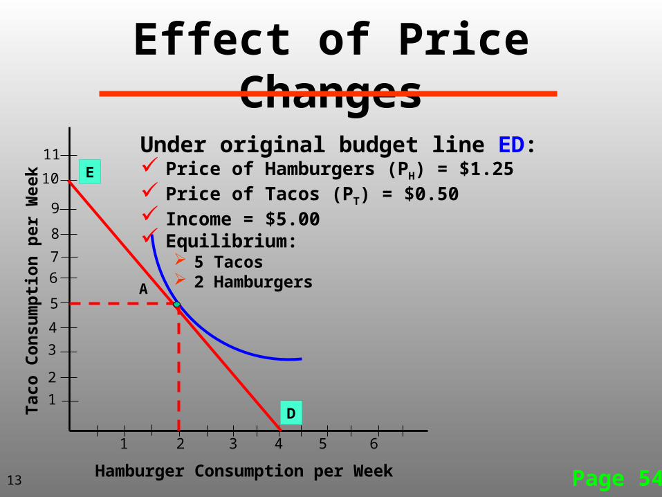
Under original budget line ED: Price of Hamburgers (PH) = $1.25 Price of Tacos (PT) = $0.50 Income = $5.00 Equilibrium:
5 Tacos 2 Hamburgers
13
A
E
Effect of Price Changes
Page 54
1 2 3 4 6
1
3
2
4
5
6
7
8
9
10
11
D
Hamburger Consumption per Week
Tac
o C
onsu
mpt
ion
per
Wee
k
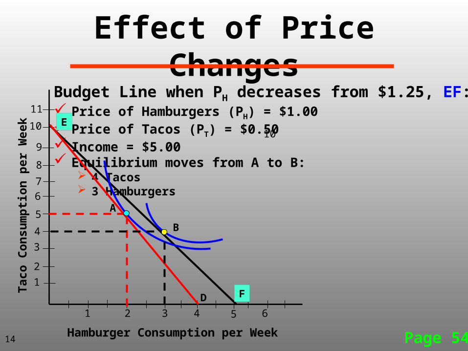
Budget Line when PH decreases from $1.25, EF: Price of Hamburgers (PH) = $1.00 Price of Tacos (PT) = $0.50 Income = $5.00 Equilibrium moves from A to B:
4 Tacos 3 Hamburgers
F
B
14
10
A
5
E
Effect of Price Changes
Page 54
1 2 3 4 6
1
3
2
4
5
6
7
8
9
10
11
D
E
Hamburger Consumption per Week
Tac
o C
onsu
mpt
ion
per
Wee
k
F
B
15
A
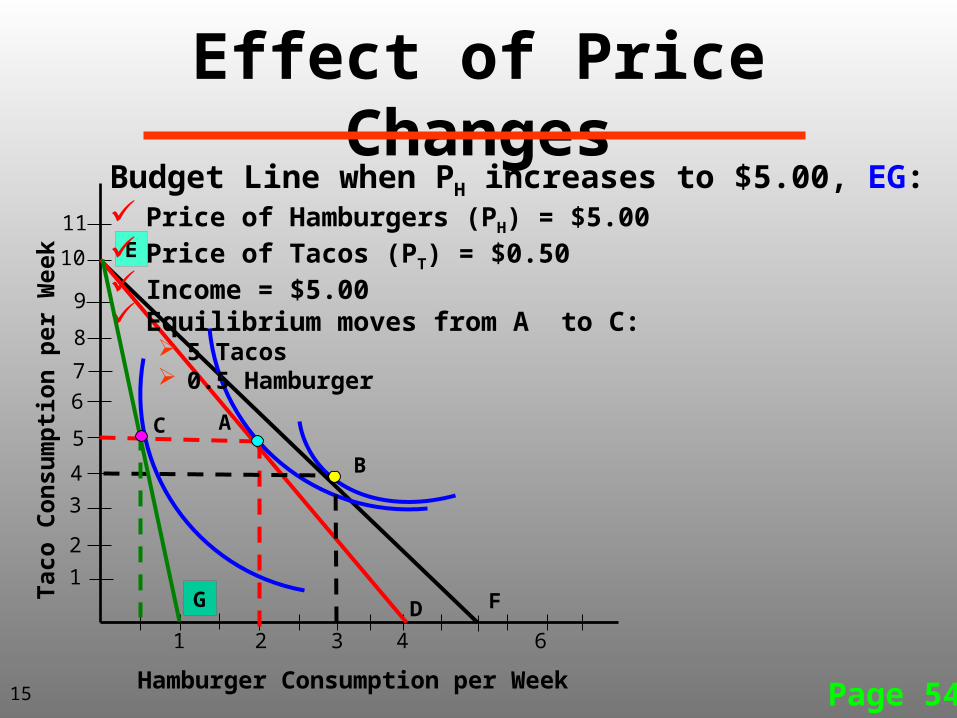
Budget Line when PH increases to $5.00, EG: Price of Hamburgers (PH) = $5.00 Price of Tacos (PT) = $0.50 Income = $5.00 Equilibrium moves from A to C:
5 Tacos 0.5 Hamburger
C
G
Effect of Price Changes
Page 54
1 2 3 4 6
1
3
2
4
5
6
7
8
9
10
11
D
E
Hamburger Consumption per Week
Tac
o C
onsu
mpt
ion
per
Wee
k
F
B
16
AC
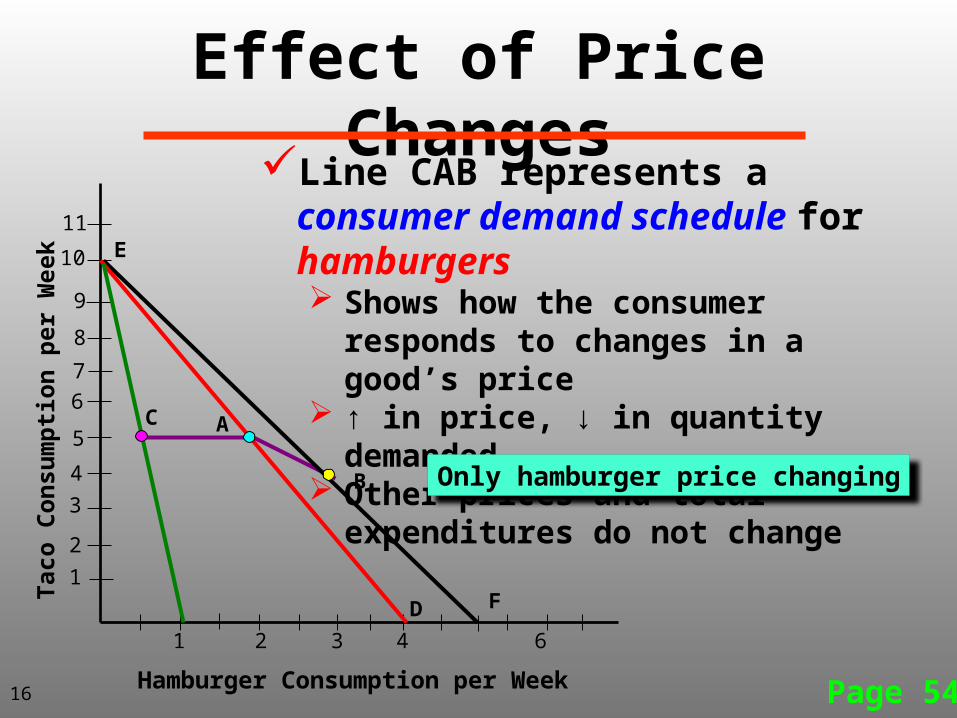
Line CAB represents a consumer demand schedule for hamburgers Shows how the consumer responds to
changes in a good’s price ↑ in price, ↓ in quantity demanded Other prices and total expenditures do not
change
Only hamburger price changing
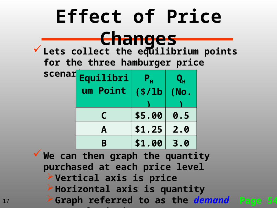
Lets collect the equilibrium points for the three hamburger price scenarios
We can then graph the quantity purchased at each price levelVertical axis is priceHorizontal axis is quantityGraph referred to as the demand curve for
hamburgers Page 54
Equilibrium Point
PH ($/lb)
QH (No.)
C $5.00 0.5
A $1.25 2.0
B $1.00 3.0
17
Effect of Price Changes
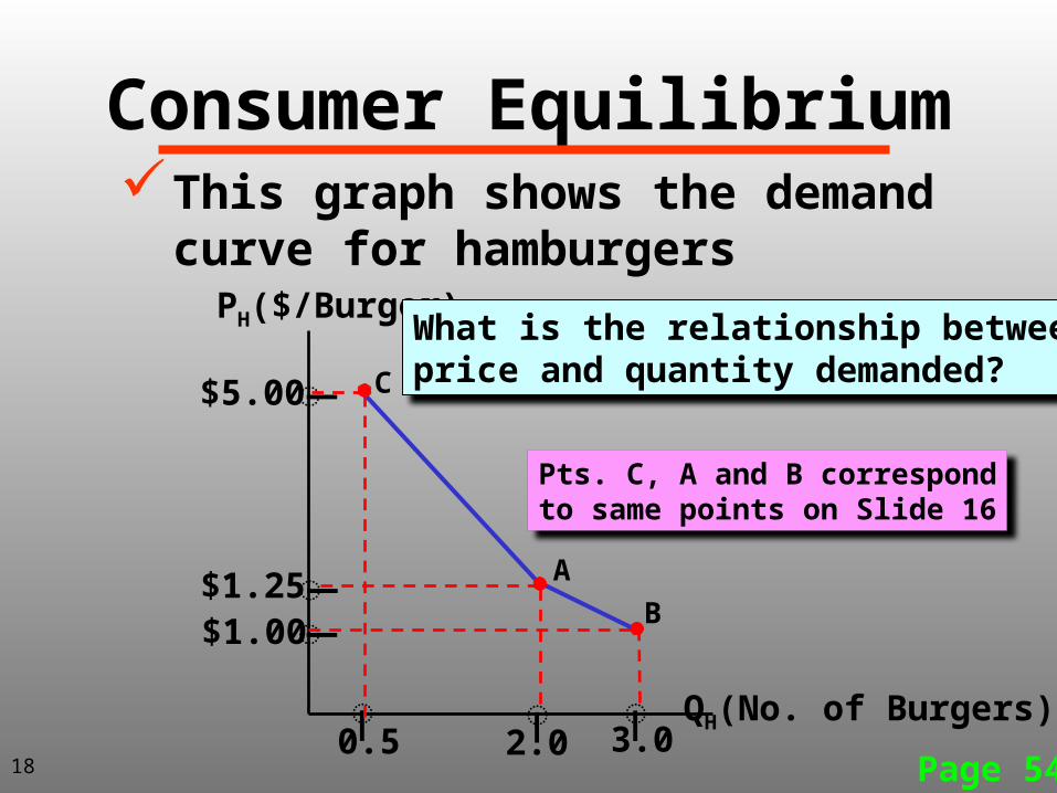
Consumer EquilibriumThis graph shows the demand curve
for hamburgers
Page 54
PH($/Burger)
H̶
H̶H̶
QH(No. of Burgers)H̶ H̶H̶
C
A
B
0.5 2.0 3.0
$5.00
$1.25$1.00
What is the relationship betweenprice and quantity demanded?
18
Pts. C, A and B correspondto same points on Slide 16
Effect of an Income Change
Page 54
1 2 3 4 5 6
1
3
2
4
5
6
7
8
9
10
11
J
K
Hamburger Consumption per Week
Tac
o C
onsu
mpt
ion
per
Wee
k
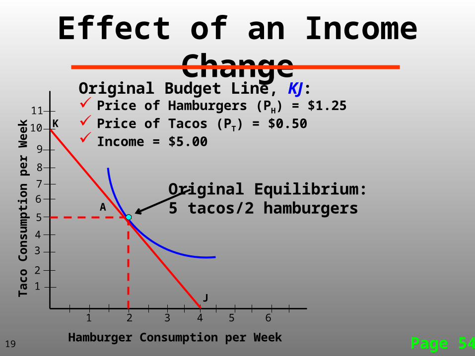
Original Budget Line, KJ: Price of Hamburgers (PH) = $1.25 Price of Tacos (PT) = $0.50 Income = $5.00
19
A
Original Equilibrium:5 tacos/2 hamburgers
Effect of an Income Change
Page 54
1 2 3 4 5 6
1
3
2
4
5
6
7
8
9
10
11
J
K
Hamburger Consumption per Week
Tac
o C
onsu
mpt
ion
per
Wee
k
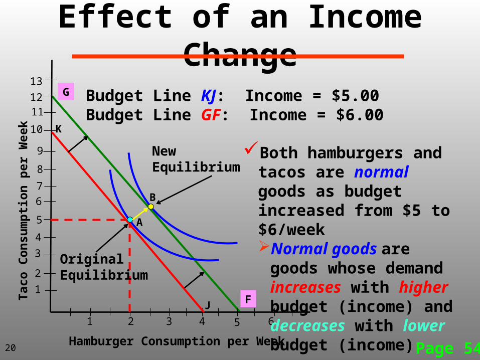
Budget Line KJ: Income = $5.00Budget Line GF: Income = $6.00
20
A
12
13
B
G
F
OriginalEquilibrium
NewEquilibrium
Both hamburgers and tacos are normal goods as budget increased from $5 to $6/weekNormal goods are goods
whose demand increases with higher budget (income) and decreases with lower budget (income)
Effect of an Income Change
Page 541 2 3 4 5 6
1
3
2
4
5
6
7
8
9
10
11
J
K
Tac
o C
onsu
mpt
ion
per
Wee
k
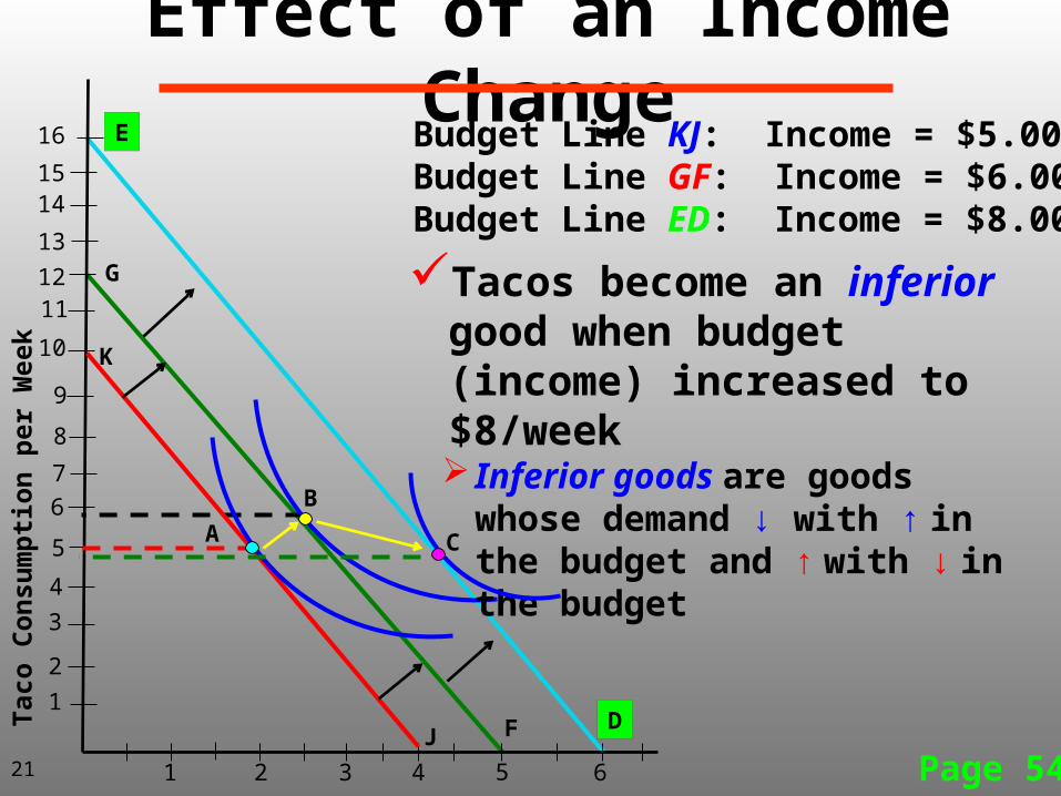
Budget Line KJ: Income = $5.00Budget Line GF: Income = $6.00Budget Line ED: Income = $8.00
21
A
12
13
B
G
F
Tacos become an inferior good when budget (income) increased to $8/week Inferior goods are goods whose
demand ↓ with ↑ in the budget and ↑ with ↓ in the budget
1415
16
C
E
D
Effect of an Income Change
Page 541 2 3 4 5 6
1
3
2
4
5
6
7
8
9
10
11
J
K
Tac
o C
onsu
mpt
ion
per
Wee
k
22
A
12
13
B
G
F
C
D
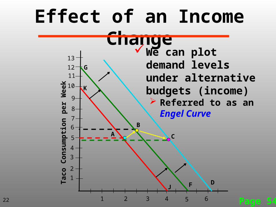
We can plot demand levels under alternative budgets (income) Referred to as an Engel
Curve
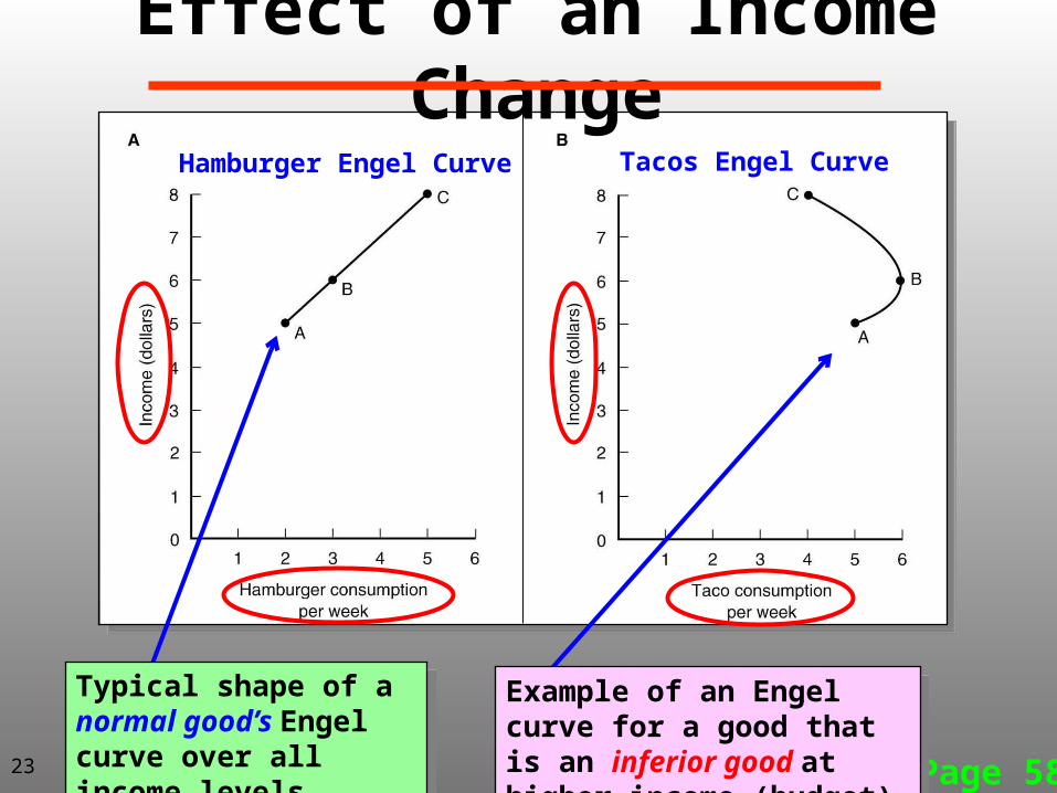
Hamburger Engel Curve Tacos Engel Curve
Page 58
Typical shape of a normal good’s Engel curve over all income levels
Typical shape of a normal good’s Engel curve over all income levels
Example of an Engel curve for a good that is an inferior good at higher income (budget) levels
Example of an Engel curve for a good that is an inferior good at higher income (budget) levels23
Effect of an Income Change

Measurement andInterpretation ofMarket Demand
24
Concept of Market DemandThe above model of consumer
behavior focused on a single individual
We can extend the above model to one where we refer to overall or total market demand for a city, county, state, country, etc.
25
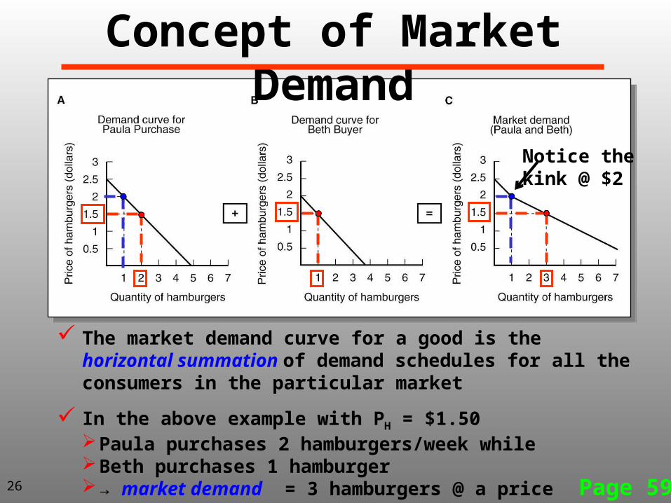
The market demand curve for a good is the horizontal summation of demand schedules for all the consumers in the particular market
In the above example with PH = $1.50Paula purchases 2 hamburgers/week while Beth purchases 1 hamburger→ market demand = 3 hamburgers @ a price $1.50/hamburger
Page 59
Concept of Market Demand
Notice thekink @ $2
26
Demand Curve DescriptionWhen discussing events in the market place
economists use specific terms to distinguish between movement along a demand curve vs. a shift in a demand curve
Movement along a demand curve referred to as a change in quantity demanded Only 1 demand curve, just a different point on it
Alternatively a shift in the demand curve referred to as a change in demandNeed not be a parallel shift in the demand curve
27
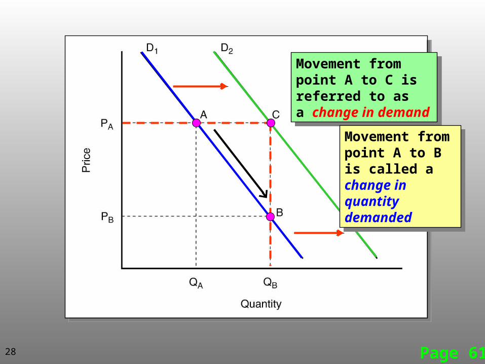
Movement from point A to C is referred to as a change in demand
Movement from point A to C is referred to as a change in demand
Page 61
Movement from point A to B is called a change in quantity demanded
Movement from point A to B is called a change in quantity demanded
28
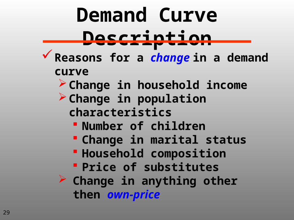
Demand Curve DescriptionReasons for a change in a demand curve
Change in household incomeChange in population characteristics
Number of children Change in marital status Household composition Price of substitutes
Change in anything other then own-price
29
Concept of Consumer SurplusA characteristic of market demand
curve Concept of consumer surplus (CS) or
economic well-being CS is derived from consumption and the
fact we have a negatively sloped demand curve (with respect to its own-price)
A demand curve reveals the willingness of consumers to pay a certain price for a particular quantity of a good
Page 63-6430
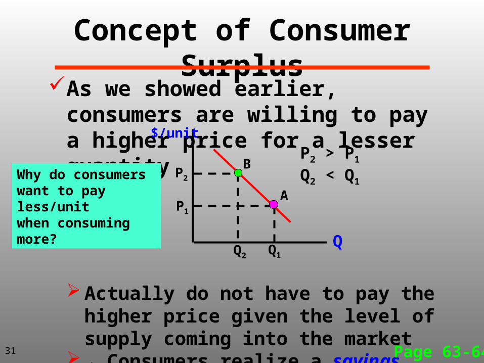
Concept of Consumer SurplusAs we showed earlier, consumers are
willing to pay a higher price for a lesser quantity
Actually do not have to pay the higher price given the level of supply coming into the market
→ Consumers realize a savingsPage 63-64
$/unit
Q
A
Q1Q2
P1
BP2
P2 > P1
Q2 < Q1
31
Why do consumerswant to pay less/unitwhen consuming more?
Page 63
Quantifying Consumer Surplus
1 2 3 4 5 6
1
3
2
4
5
6
7
8
9
10
11
7 8 9 10 110
AC
B
ED
32
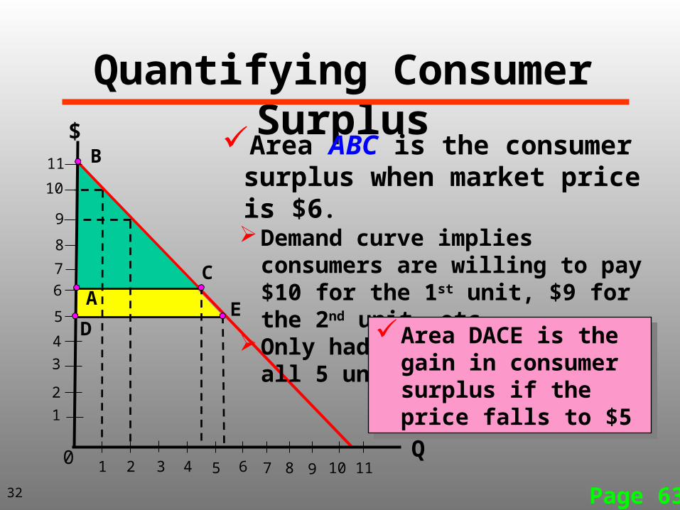
Area ABC is the consumer surplus when market price is $6. Demand curve implies consumers are
willing to pay $10 for the 1st unit, $9 for the 2nd unit, etc.
Only had to pay $6 each for all 5 units
Area DACE is the gain in consumer surplus if the price falls to $5
Area DACE is the gain in consumer surplus if the price falls to $5
Q
$
33 Page 63
Quantifying Consumer Surplus
1 2 3 4 5 6
1
3
2
4
5
6
7
8
9
10
11
7 8 9 10 110
A C
B
ED
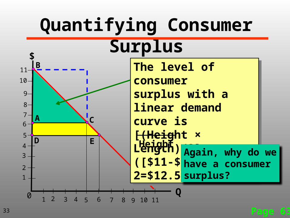
The level of consumersurplus with a linear demand curve is [(Height × Length)/2] =([$11-$6]×5)/2=$12.50
The level of consumersurplus with a linear demand curve is [(Height × Length)/2] =([$11-$6]×5)/2=$12.50
Q
$
HeightAgain, why do wehave a consumersurplus?
In SummaryConsumer equilibrium for an
individual for a given price and budgetIndividual consumer’s demand
scheduleMarket demand curveEngel curvesChange in demand vs. change in
quantity demandedConsumer surplus

Chapter 5 examines the concept of an elasticity, one of the most important concepts in all of economics….