Embed Size (px)
Citation preview
Demand, Supply and Equilibrium
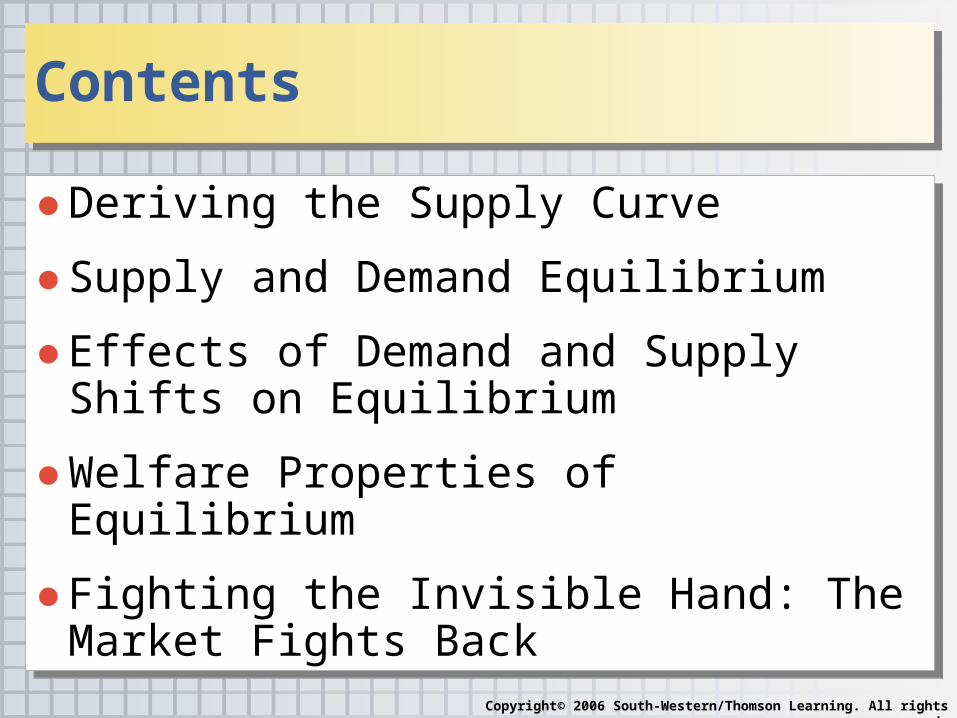
● Deriving the Supply Curve
● Supply and Demand Equilibrium
● Effects of Demand and Supply Shifts on Equilibrium
● Welfare Properties of Equilibrium
● Fighting the Invisible Hand: The Market Fights Back
● Deriving the Supply Curve
● Supply and Demand Equilibrium
● Effects of Demand and Supply Shifts on Equilibrium
● Welfare Properties of Equilibrium
● Fighting the Invisible Hand: The Market Fights Back
ContentsContents
Copyright© 2006 South-Western/Thomson Learning. All rights reserved.
Copyright© 2006 South-Western/Thomson Learning. All rights reserved.
The Invisible Hand The Invisible Hand
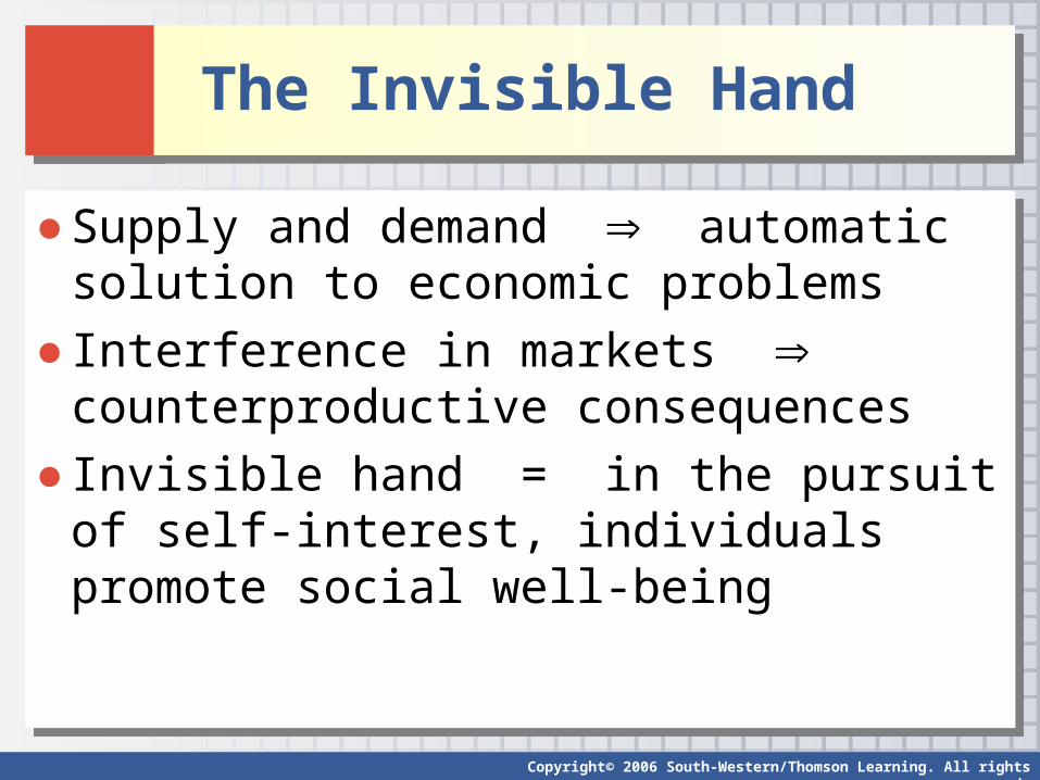
● Supply and demand automatic solution to economic problems
● Interference in markets counterproductive consequences
● Invisible hand = in the pursuit of self-interest, individuals promote social well-being
● Supply and demand automatic solution to economic problems
● Interference in markets counterproductive consequences
● Invisible hand = in the pursuit of self-interest, individuals promote social well-being
Copyright© 2006 South-Western/Thomson Learning. All rights reserved.
Deriving Supply Curve Deriving Supply Curve
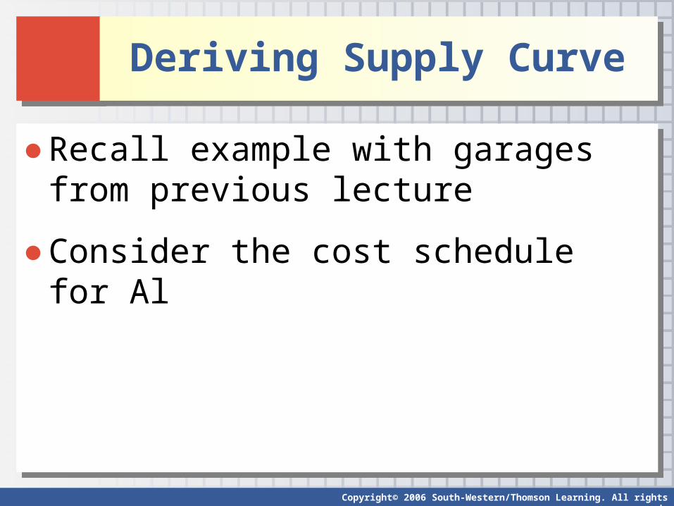
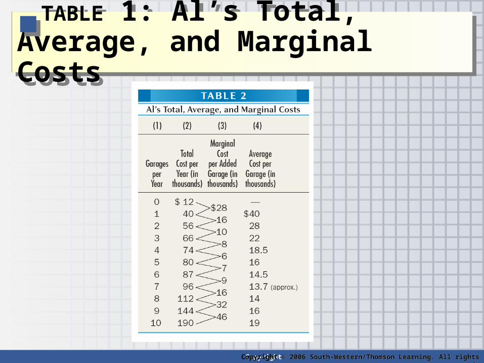
● Recall example with garages from previous lecture
● Consider the cost schedule for Al
● Recall example with garages from previous lecture
● Consider the cost schedule for Al
Copyright© 2006 South-Western/Thomson Learning. All rights reserved.
TABLE 1: Al’s Total, Average, and Marginal Costs
TABLE 1: Al’s Total, Average, and Marginal Costs
Copyright © 2006 South-Western/Thomson Learning. All rights reserved.
Copyright© 2006 South-Western/Thomson Learning. All rights reserved.
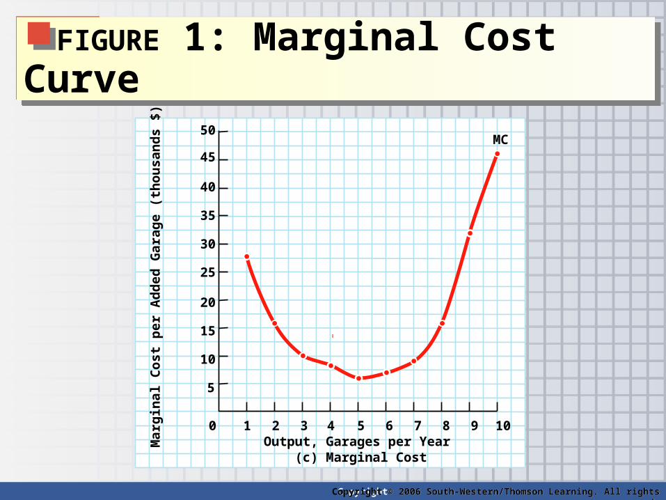
FIGURE 1: Marginal Cost CurveFIGURE 1: Marginal Cost Curve
Copyright © 2006 South-Western/Thomson Learning. All rights reserved.
MC
(c) Marginal Cost Output, Garages per Year
5
Mar
gin
al
Co
st p
er A
dd
ed G
arag
e (t
ho
usa
nd
s $
)
10 9 8 7 6 4 3 2 1 0
5
10
15
45
50
40
35
30
25
20
Copyright© 2006 South-Western/Thomson Learning. All rights reserved.
Supply CurveSupply Curve
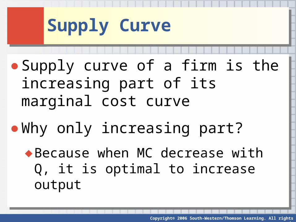
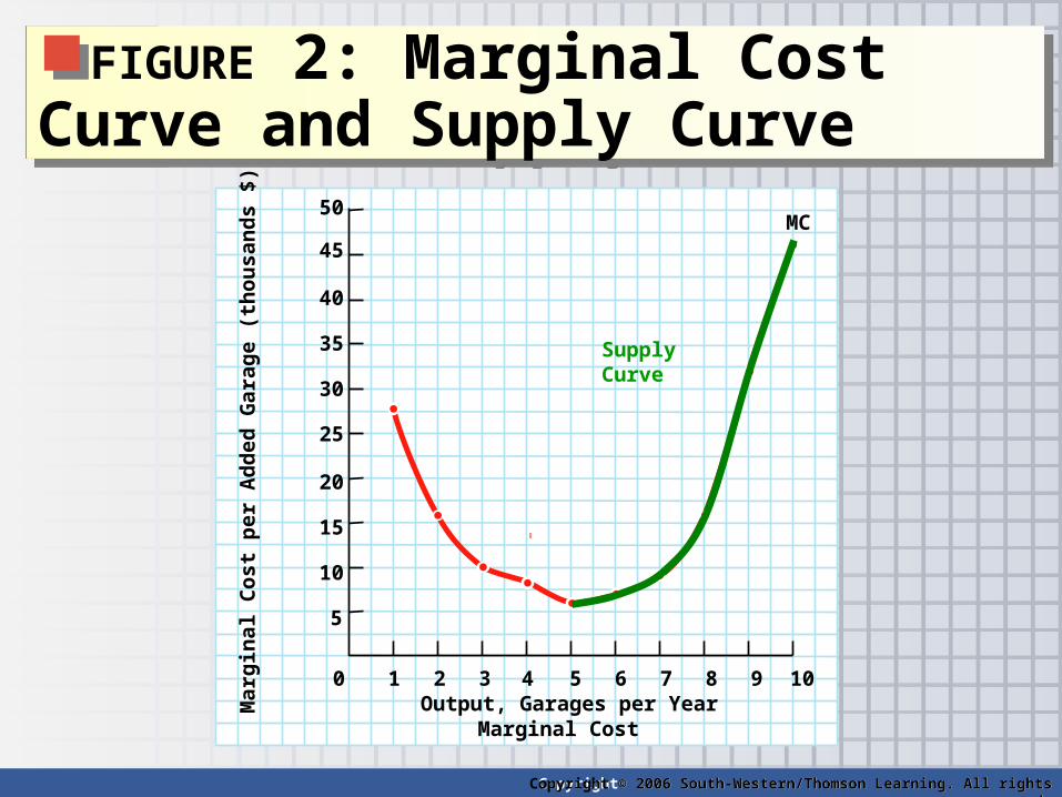
● Supply curve of a firm is the increasing part of its marginal cost curve
● Why only increasing part?
♦ Because when MC decrease with Q, it is optimal to increase output
● Supply curve of a firm is the increasing part of its marginal cost curve
● Why only increasing part?
♦ Because when MC decrease with Q, it is optimal to increase output
Copyright© 2006 South-Western/Thomson Learning. All rights reserved.
FIGURE 2: Marginal Cost Curve and Supply Curve
FIGURE 2: Marginal Cost Curve and Supply Curve
Copyright © 2006 South-Western/Thomson Learning. All rights reserved.
MC
Marginal Cost Output, Garages per Year
5
Mar
gin
al
Co
st p
er A
dd
ed G
arag
e (t
ho
usa
nd
s $
)
10 9 8 7 6 4 3 2 1 0
5
10
15
45
50
40
35
30
25
20
Supply Curve
Copyright© 2006 South-Western/Thomson Learning. All rights reserved.
From Individual to Market SupplyFrom Individual to Market Supply
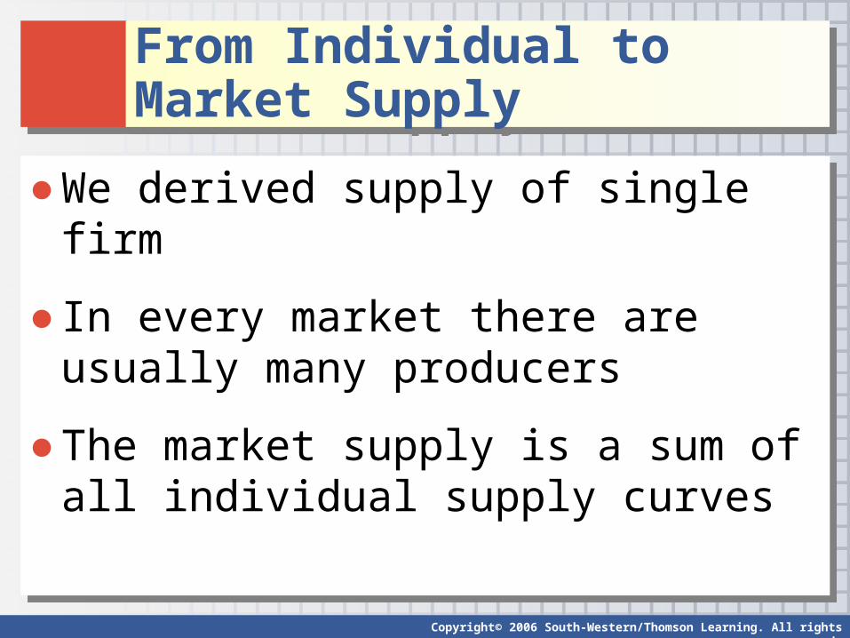
● We derived supply of single firm
● In every market there are usually many producers
● The market supply is a sum of all individual supply curves
● We derived supply of single firm
● In every market there are usually many producers
● The market supply is a sum of all individual supply curves
Copyright© 2006 South-Western/Thomson Learning. All rights reserved.
Supply and Quantity SuppliedSupply and Quantity Supplied
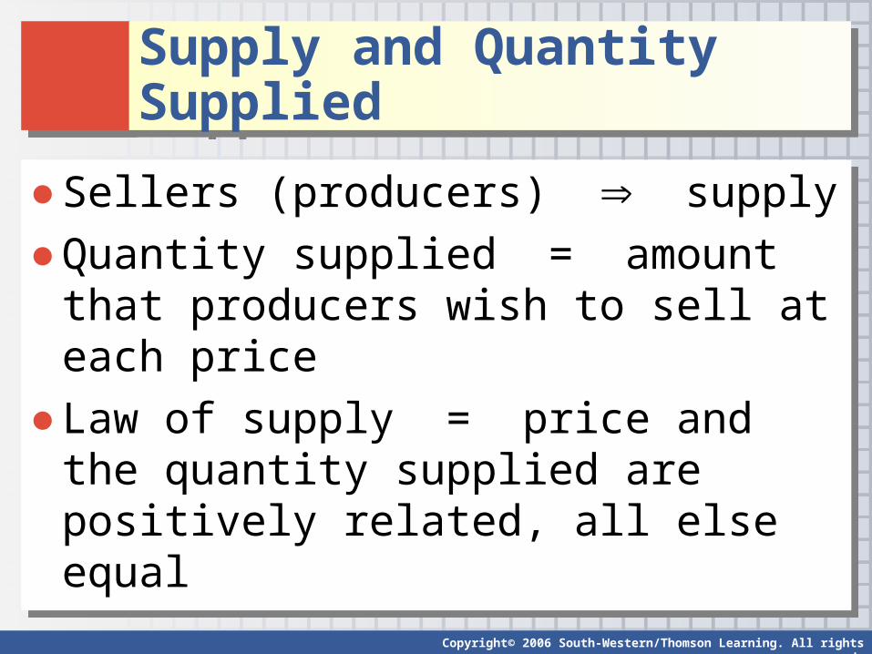
● Sellers (producers) supply
● Quantity supplied = amount that producers wish to sell at each price
● Law of supply = price and the quantity supplied are positively related, all else equal
● Sellers (producers) supply
● Quantity supplied = amount that producers wish to sell at each price
● Law of supply = price and the quantity supplied are positively related, all else equal
Copyright© 2006 South-Western/Thomson Learning. All rights reserved.
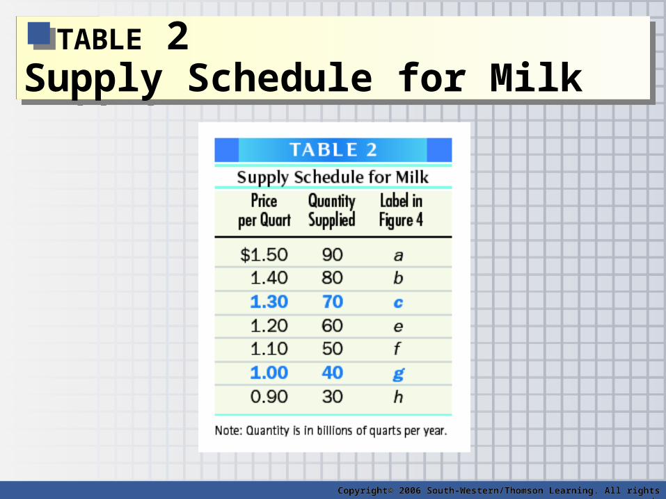
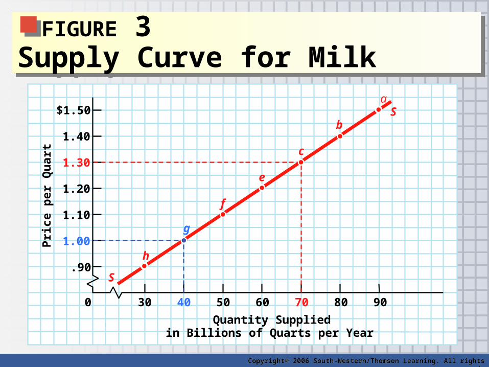
TABLE 2 Supply Schedule for Milk
TABLE 2 Supply Schedule for Milk
Copyright© 2006 South-Western/Thomson Learning. All rights reserved.
Copyright© 2006 South-Western/Thomson Learning. All rights reserved.
Supply and Quantity SuppliedSupply and Quantity Supplied
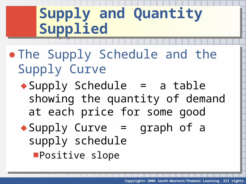
● The Supply Schedule and the Supply Curve♦ Supply Schedule = a table showing the
quantity of demand at each price for some good
♦ Supply Curve = graph of a supply schedule■Positive slope
● The Supply Schedule and the Supply Curve♦ Supply Schedule = a table showing the
quantity of demand at each price for some good
♦ Supply Curve = graph of a supply schedule■Positive slope
Copyright© 2006 South-Western/Thomson Learning. All rights reserved.
FIGURE 3 Supply Curve for Milk
FIGURE 3 Supply Curve for Milk
S
S
a
b
c
e
f
g
h
90 80 70 60 50 40
$1.50
1.40
1.30
1.20
1.10
1.00
Pri
ce
pe
r Q
uar
t
Quantity Supplied in Billions of Quarts per Year
30 0
.90
Copyright© 2006 South-Western/Thomson Learning. All rights reserved.
Copyright© 2006 South-Western/Thomson Learning. All rights reserved.
Supply and Quantity SuppliedSupply and Quantity Supplied
● Shifts of the Supply Curve♦ Movement along a supply curve due to
■Changes in price
♦ Shift between supply curves due to■Changes in industry size (entry and exit)■Changes in production technology■Changes in prices of inputs■Changes in prices of related outputs
● Shifts of the Supply Curve♦ Movement along a supply curve due to
■Changes in price
♦ Shift between supply curves due to■Changes in industry size (entry and exit)■Changes in production technology■Changes in prices of inputs■Changes in prices of related outputs
Copyright© 2006 South-Western/Thomson Learning. All rights reserved.
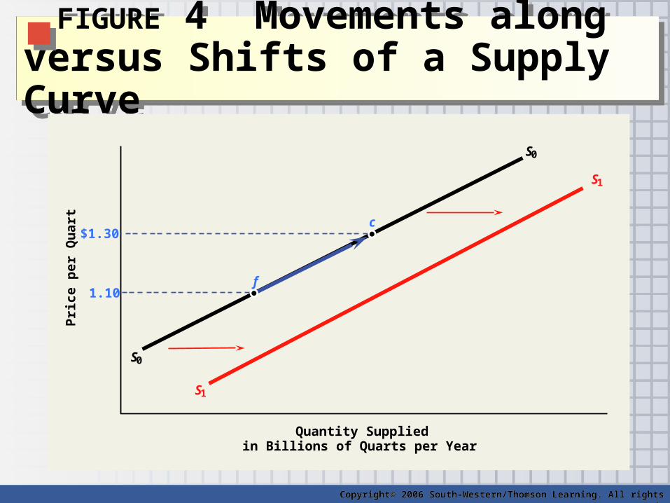
FIGURE 4 Movements along versus Shifts of a Supply Curve
FIGURE 4 Movements along versus Shifts of a Supply Curve
S0
S0
Pri
ce p
er Q
uar
t
Quantity Supplied in Billions of Quarts per Year
c
f
S1
S1
1.10
$1.30
Copyright© 2006 South-Western/Thomson Learning. All rights reserved.
Copyright© 2006 South-Western/Thomson Learning. All rights reserved.
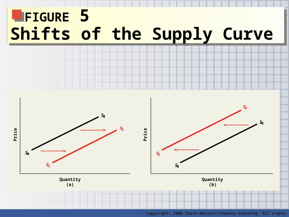
FIGURE 5 Shifts of the Supply Curve
FIGURE 5 Shifts of the Supply Curve
S2
S2
S0
S0
Quantity (b)
S1
S1
S0
S0
Pri
ce
Pri
ce
Quantity (a)
Copyright© 2006 South-Western/Thomson Learning. All rights reserved.
Copyright© 2006 South-Western/Thomson Learning. All rights reserved.
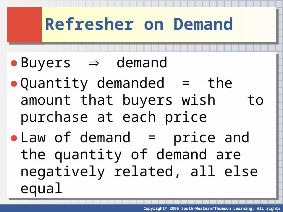
Refresher on DemandRefresher on Demand
● Buyers demand
● Quantity demanded = the amount that buyers wish to purchase at each price
● Law of demand = price and the quantity of demand are negatively related, all else equal
● Buyers demand
● Quantity demanded = the amount that buyers wish to purchase at each price
● Law of demand = price and the quantity of demand are negatively related, all else equal
Copyright© 2006 South-Western/Thomson Learning. All rights reserved.
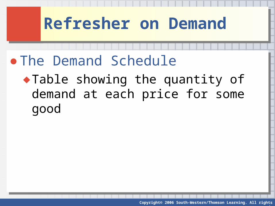
Refresher on DemandRefresher on Demand
● The Demand Schedule♦ Table showing the quantity of demand at each
price for some good
● The Demand Schedule♦ Table showing the quantity of demand at each
price for some good
Copyright© 2006 South-Western/Thomson Learning. All rights reserved.
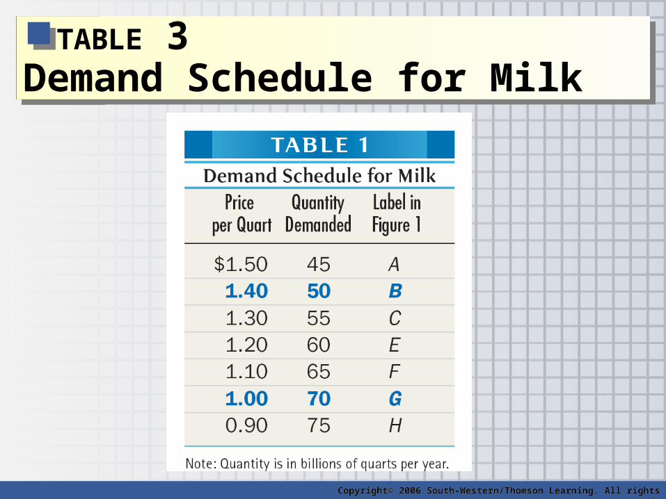
TABLE 3 Demand Schedule for Milk
TABLE 3 Demand Schedule for Milk
Copyright© 2006 South-Western/Thomson Learning. All rights reserved.
Copyright© 2006 South-Western/Thomson Learning. All rights reserved.
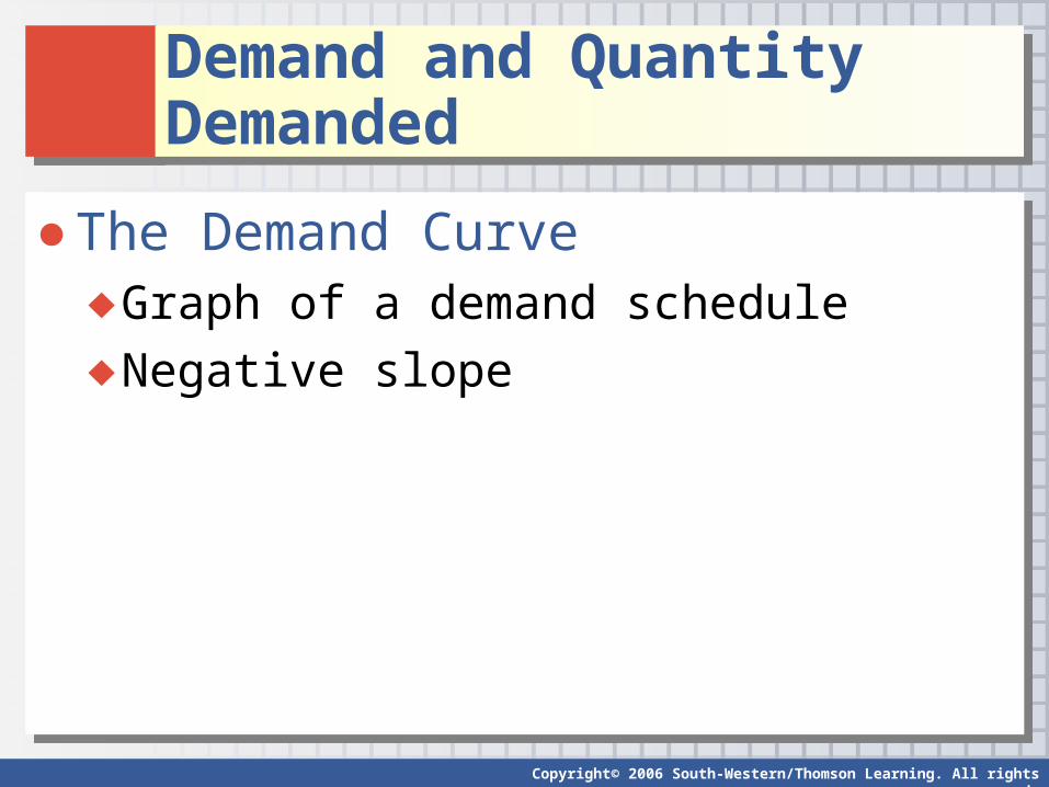
● The Demand Curve♦ Graph of a demand schedule
♦ Negative slope
● The Demand Curve♦ Graph of a demand schedule
♦ Negative slope
Demand and Quantity DemandedDemand and Quantity Demanded
Copyright© 2006 South-Western/Thomson Learning. All rights reserved.
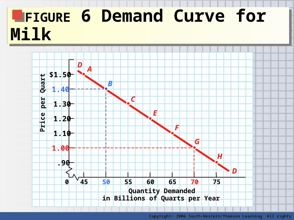
FIGURE 6 Demand Curve for MilkFIGURE 6 Demand Curve for MilkP
rice
per
Qu
art
H
G
F
E
C
D
D
B
A
Quantity Demanded in Billions of Quarts per Year
75 70 65 60 55 50 45 0
.90
1.00
1.10
1.20
1.30
1.40
$1.50
Copyright© 2006 South-Western/Thomson Learning. All rights reserved.
Copyright© 2006 South-Western/Thomson Learning. All rights reserved.
Demand and Quantity DemandedDemand and Quantity Demanded
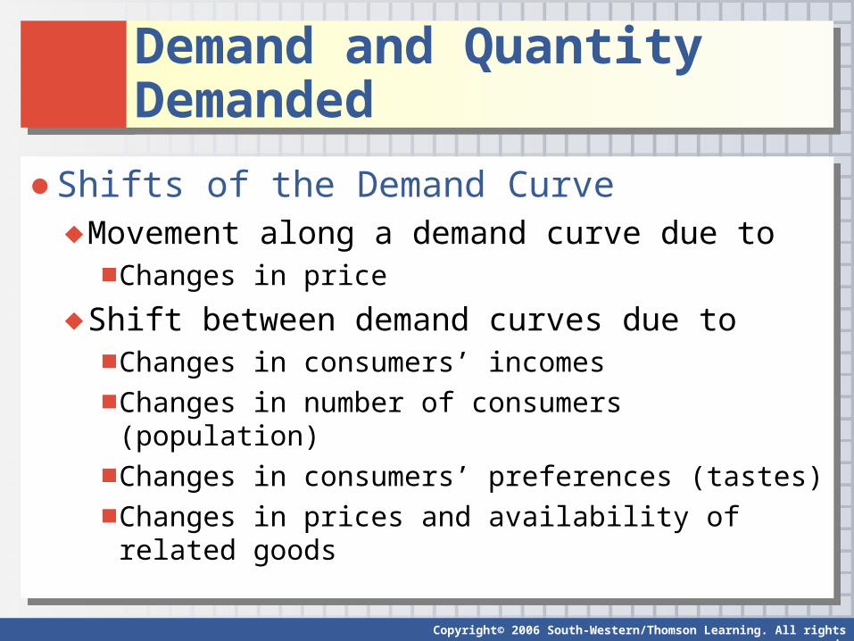
● Shifts of the Demand Curve♦ Movement along a demand curve due to
■Changes in price
♦ Shift between demand curves due to■Changes in consumers’ incomes■Changes in number of consumers (population)■Changes in consumers’ preferences (tastes)■Changes in prices and availability of related goods
● Shifts of the Demand Curve♦ Movement along a demand curve due to
■Changes in price
♦ Shift between demand curves due to■Changes in consumers’ incomes■Changes in number of consumers (population)■Changes in consumers’ preferences (tastes)■Changes in prices and availability of related goods
Copyright© 2006 South-Western/Thomson Learning. All rights reserved.
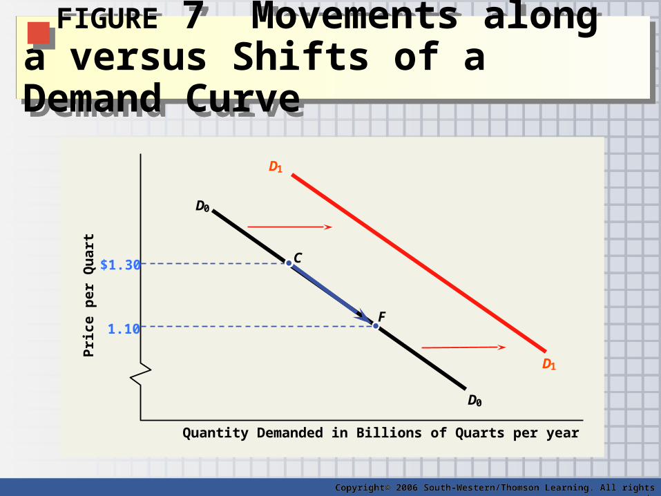
FIGURE 7 Movements along a versus Shifts of a Demand Curve
FIGURE 7 Movements along a versus Shifts of a Demand Curve
Pri
ce
pe
r Q
ua
rt
Quantity Demanded in Billions of Quarts per year
F 1.10
$1.30
D0
D0
C
D1
D1
Copyright© 2006 South-Western/Thomson Learning. All rights reserved.
Copyright© 2006 South-Western/Thomson Learning. All rights reserved.
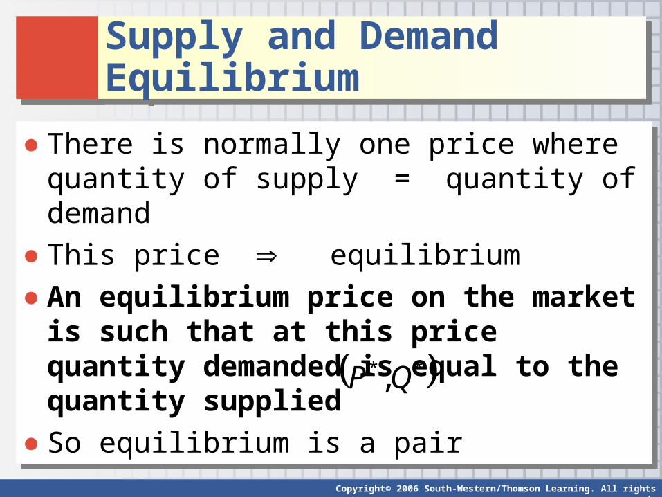
Supply and Demand EquilibriumSupply and Demand Equilibrium
● There is normally one price where quantity of supply = quantity of demand
● This price equilibrium
● An equilibrium price on the market is such that at this price quantity demanded is equal to the quantity supplied
● So equilibrium is a pair
● There is normally one price where quantity of supply = quantity of demand
● This price equilibrium
● An equilibrium price on the market is such that at this price quantity demanded is equal to the quantity supplied
● So equilibrium is a pair **,QP
Copyright© 2006 South-Western/Thomson Learning. All rights reserved.
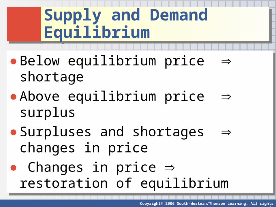
Supply and Demand EquilibriumSupply and Demand Equilibrium
● Below equilibrium price shortage
● Above equilibrium price surplus
● Surpluses and shortages changes in price
● Changes in price restoration of equilibrium
● Below equilibrium price shortage
● Above equilibrium price surplus
● Surpluses and shortages changes in price
● Changes in price restoration of equilibrium

TABLE 4 Equilibrium Price & Quantity of Milk
TABLE 4 Equilibrium Price & Quantity of Milk
Copyright© 2006 South-Western/Thomson Learning. All rights reserved.
Copyright© 2006 South-Western/Thomson Learning. All rights reserved.
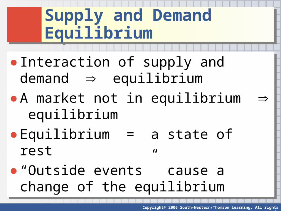
Supply and Demand EquilibriumSupply and Demand Equilibrium
● Interaction of supply and demand equilibrium
● A market not in equilibrium equilibrium
● Equilibrium = a state of rest
● “Outside events” cause a change of the equilibrium
● Interaction of supply and demand equilibrium
● A market not in equilibrium equilibrium
● Equilibrium = a state of rest
● “Outside events” cause a change of the equilibrium
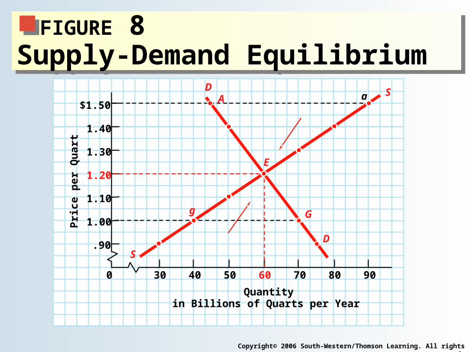
FIGURE 8 Supply-Demand Equilibrium
FIGURE 8 Supply-Demand Equilibrium
D
D
G
A S
S
90 80 70 60 50 40
$1.50
1.40
1.30
1.20
1.10
1.00
Pri
ce p
er Q
uar
t
Quantity in Billions of Quarts per Year
30 0
.90
E
g
a
Copyright© 2006 South-Western/Thomson Learning. All rights reserved.
Copyright© 2006 South-Western/Thomson Learning. All rights reserved.
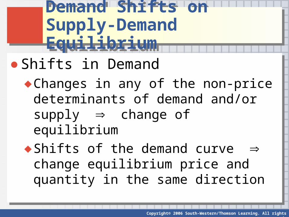
Demand Shifts on Supply-Demand EquilibriumDemand Shifts on Supply-Demand Equilibrium
● Shifts in Demand♦ Changes in any of the non-price determinants
of demand and/or supply change of equilibrium
♦ Shifts of the demand curve change equilibrium price and quantity in the same direction
● Shifts in Demand♦ Changes in any of the non-price determinants
of demand and/or supply change of equilibrium
♦ Shifts of the demand curve change equilibrium price and quantity in the same direction
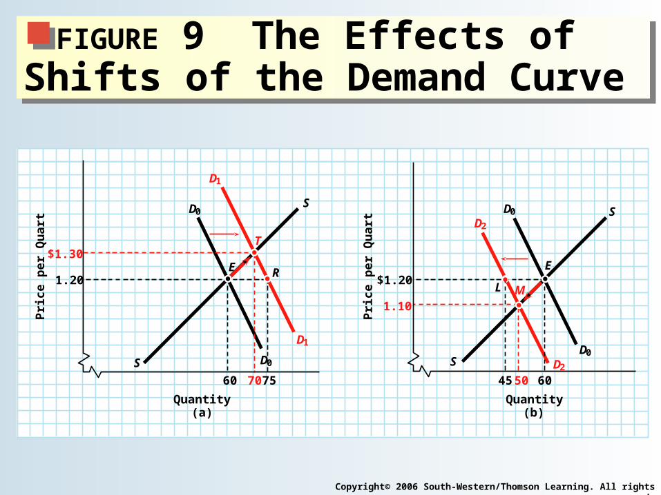
FIGURE 9 The Effects of Shifts of the Demand Curve
FIGURE 9 The Effects of Shifts of the Demand Curve
60
(b)
60 45 50
1.10
Quantity
$1.20
(a)
75 70
$1.30
Pri
ce p
er Q
uar
t
Pri
ce p
er Q
uar
t
Quantity
1.20
D0
D0
D1
D1
S
S
T
R E
D2
D2
D0
D0
S
S
M
E
L
Copyright© 2006 South-Western/Thomson Learning. All rights reserved.
Copyright© 2006 South-Western/Thomson Learning. All rights reserved.
Supply Shifts and Supply-Demand EquilibriumSupply Shifts and Supply-Demand Equilibrium
● Shifts in Supply♦ Shifts of the supply curve change in
equilibrium price and quantity in opposite directions
♦ Old equilibrium position new equilibrium position
● Shifts in Supply♦ Shifts of the supply curve change in
equilibrium price and quantity in opposite directions
♦ Old equilibrium position new equilibrium position
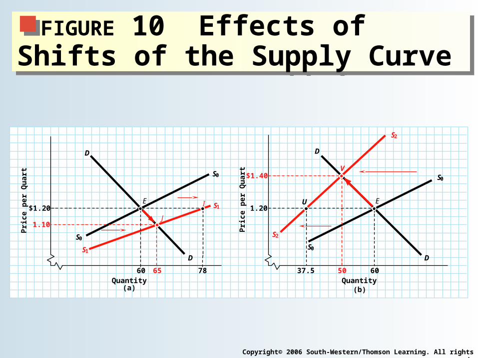
FIGURE 10 Effects of Shifts of the Supply Curve
FIGURE 10 Effects of Shifts of the Supply Curve
D
D
S2
S2
S0
S0
37.5 50
(b)
60
$1.40
Quantity
1.20
D
D S1
S1
S0
S0
78 65
(a)
60
1.10 Pri
ce p
er Q
uar
t
Pri
ce p
er Q
uar
t
Quantity
$1.20
V
U E
J
I E
Copyright© 2006 South-Western/Thomson Learning. All rights reserved.
Copyright© 2006 South-Western/Thomson Learning. All rights reserved.
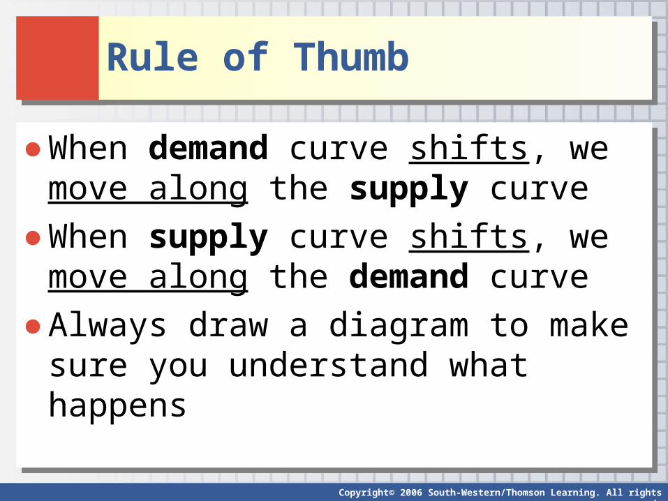
Rule of ThumbRule of Thumb
● When demand curve shifts, we move along the supply curve
● When supply curve shifts, we move along the demand curve
● Always draw a diagram to make sure you understand what happens
● When demand curve shifts, we move along the supply curve
● When supply curve shifts, we move along the demand curve
● Always draw a diagram to make sure you understand what happens
Copyright© 2006 South-Western/Thomson Learning. All rights reserved.
Sometimes we cannot say much…Sometimes we cannot say much…
● When both supply and demand curve shift, we usually have problems with predicting new equilibium:♦ Can predict price, not quantity
♦ Or can predict quantity, not price
● Because it is the degree of shifts in both curves that determine the final outcome
● When both supply and demand curve shift, we usually have problems with predicting new equilibium:♦ Can predict price, not quantity
♦ Or can predict quantity, not price
● Because it is the degree of shifts in both curves that determine the final outcome
Copyright© 2006 South-Western/Thomson Learning. All rights reserved.
Consumer SurplusConsumer Surplus
● Consumer Surplus is the difference between the maximum amount that the consumer is willing to pay for the product and the price that she actually gets to pay
● Graphically it is the area above the equilibrium price and below the market demand line
● Consumer Surplus is the difference between the maximum amount that the consumer is willing to pay for the product and the price that she actually gets to pay
● Graphically it is the area above the equilibrium price and below the market demand line
Copyright© 2006 South-Western/Thomson Learning. All rights reserved.
Producer SurplusProducer Surplus
● Producer Surplus is the difference between the price at which the producer happens to sell the product and her costs (i.e. the smallest amount of money she is willing to accept in exchange for the product she offers)
● Graphically it is the area below the equilibrium price and above the market supply line
Copyright© 2006 South-Western/Thomson Learning. All rights reserved.
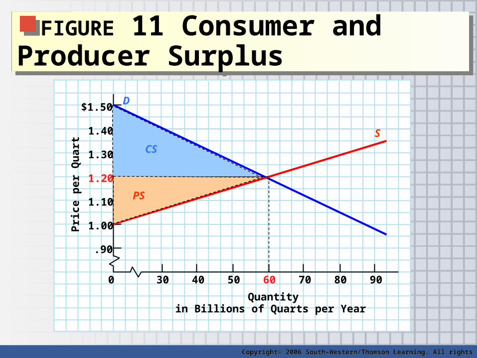
FIGURE 11 Consumer and Producer Surplus
FIGURE 11 Consumer and Producer Surplus
90 80 70 60 50 40
$1.50
1.40
1.30
1.20
1.10
1.00
Pri
ce p
er Q
uar
t
Quantity in Billions of Quarts per Year
30 0
.90
Copyright© 2006 South-Western/Thomson Learning. All rights reserved.
D
S
CS
PS
Copyright© 2006 South-Western/Thomson Learning. All rights reserved.
Some Geometry RefresherSome Geometry Refresher
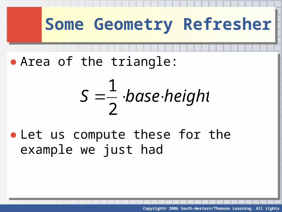
● Area of the triangle:
● Let us compute these for the example we just had
● Area of the triangle:
● Let us compute these for the example we just had
heightbaseS 2
1
Copyright© 2006 South-Western/Thomson Learning. All rights reserved.
Calculating CS and PSCalculating CS and PS
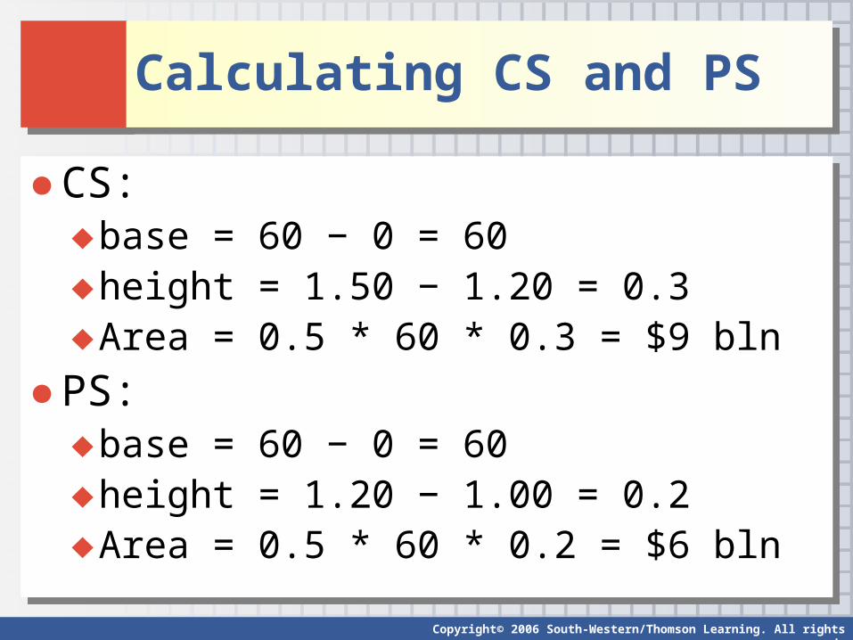
● CS:♦ base = 60 − 0 = 60♦ height = 1.50 − 1.20 = 0.3♦ Area = 0.5 * 60 * 0.3 = $9 bln
● PS:♦ base = 60 − 0 = 60♦ height = 1.20 − 1.00 = 0.2♦ Area = 0.5 * 60 * 0.2 = $6 bln
● CS:♦ base = 60 − 0 = 60♦ height = 1.50 − 1.20 = 0.3♦ Area = 0.5 * 60 * 0.3 = $9 bln
● PS:♦ base = 60 − 0 = 60♦ height = 1.20 − 1.00 = 0.2♦ Area = 0.5 * 60 * 0.2 = $6 bln
Copyright© 2006 South-Western/Thomson Learning. All rights reserved.
Total Surplus and WelfareTotal Surplus and Welfare
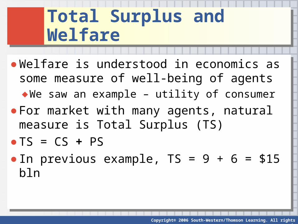
● Welfare is understood in economics as some measure of well-being of agents♦ We saw an example – utility of consumer
● For market with many agents, natural measure is Total Surplus (TS)
● TS = CS + PS
● In previous example, TS = 9 + 6 = $15 bln
● Welfare is understood in economics as some measure of well-being of agents♦ We saw an example – utility of consumer
● For market with many agents, natural measure is Total Surplus (TS)
● TS = CS + PS
● In previous example, TS = 9 + 6 = $15 bln
Copyright© 2006 South-Western/Thomson Learning. All rights reserved.
Why Market Economy?Why Market Economy?
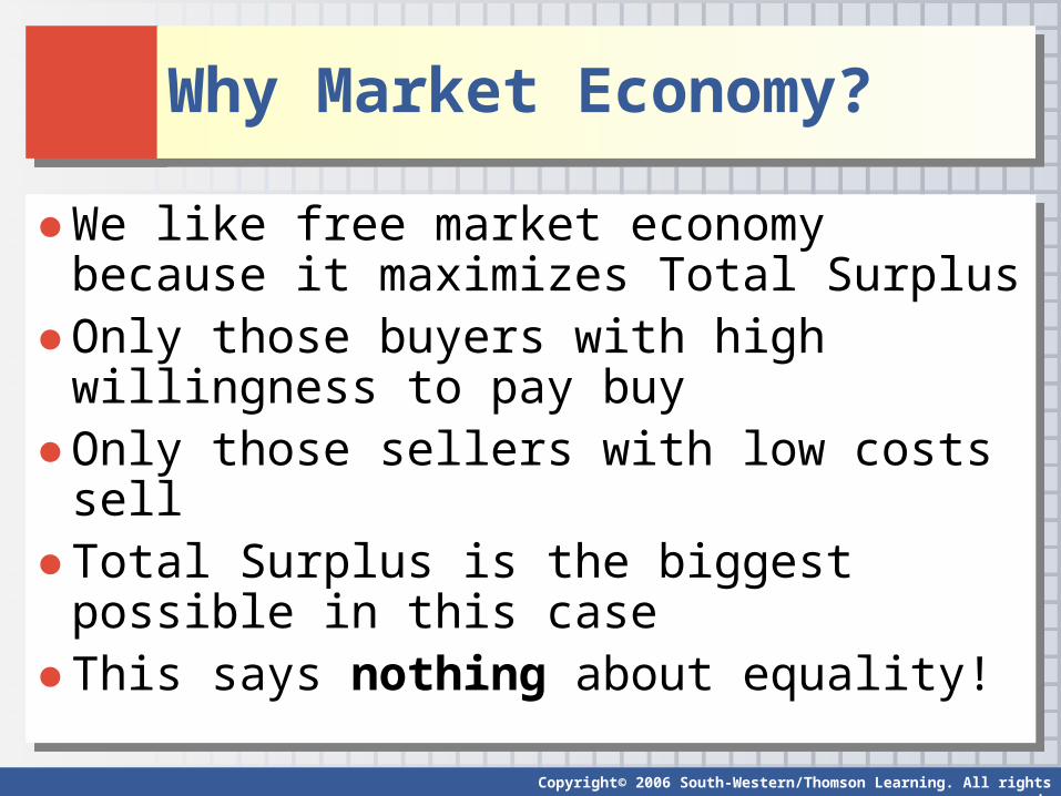
● We like free market economy because it maximizes Total Surplus
● Only those buyers with high willingness to pay buy
● Only those sellers with low costs sell● Total Surplus is the biggest possible in this
case● This says nothing about equality!
● We like free market economy because it maximizes Total Surplus
● Only those buyers with high willingness to pay buy
● Only those sellers with low costs sell● Total Surplus is the biggest possible in this
case● This says nothing about equality!

Copyright© 2006 South-Western/Thomson Learning. All rights reserved.
Fighting the Invisible Hand: The Market Fights BackFighting the Invisible Hand: The Market Fights Back
● A Can of Worms♦ Favoritism and corruption
♦ Unenforceability
♦ Limitation of the volume of transactions
♦ Misallocation of resources
● Let us see what our model predicts about fighting the invisible hand
● A Can of Worms♦ Favoritism and corruption
♦ Unenforceability
♦ Limitation of the volume of transactions
♦ Misallocation of resources
● Let us see what our model predicts about fighting the invisible hand
Copyright© 2006 South-Western/Thomson Learning. All rights reserved.
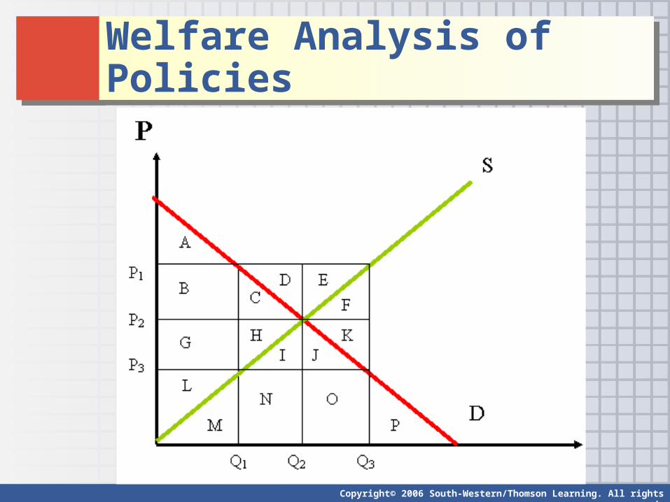
Welfare Analysis of PoliciesWelfare Analysis of Policies
Copyright© 2006 South-Western/Thomson Learning. All rights reserved.
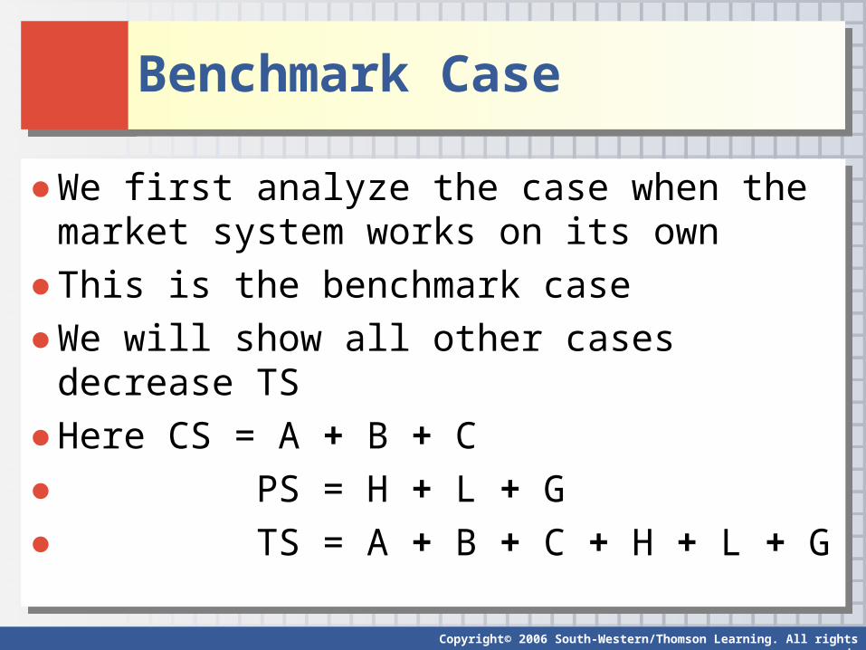
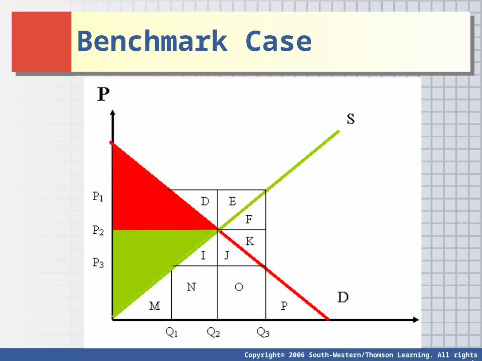
Benchmark CaseBenchmark Case
● We first analyze the case when the market system works on its own
● This is the benchmark case
● We will show all other cases decrease TS
● Here CS = A + B + C
● PS = H + L + G
● TS = A + B + C + H + L + G
● We first analyze the case when the market system works on its own
● This is the benchmark case
● We will show all other cases decrease TS
● Here CS = A + B + C
● PS = H + L + G
● TS = A + B + C + H + L + G
Copyright© 2006 South-Western/Thomson Learning. All rights reserved.
Benchmark CaseBenchmark Case
Copyright© 2006 South-Western/Thomson Learning. All rights reserved.
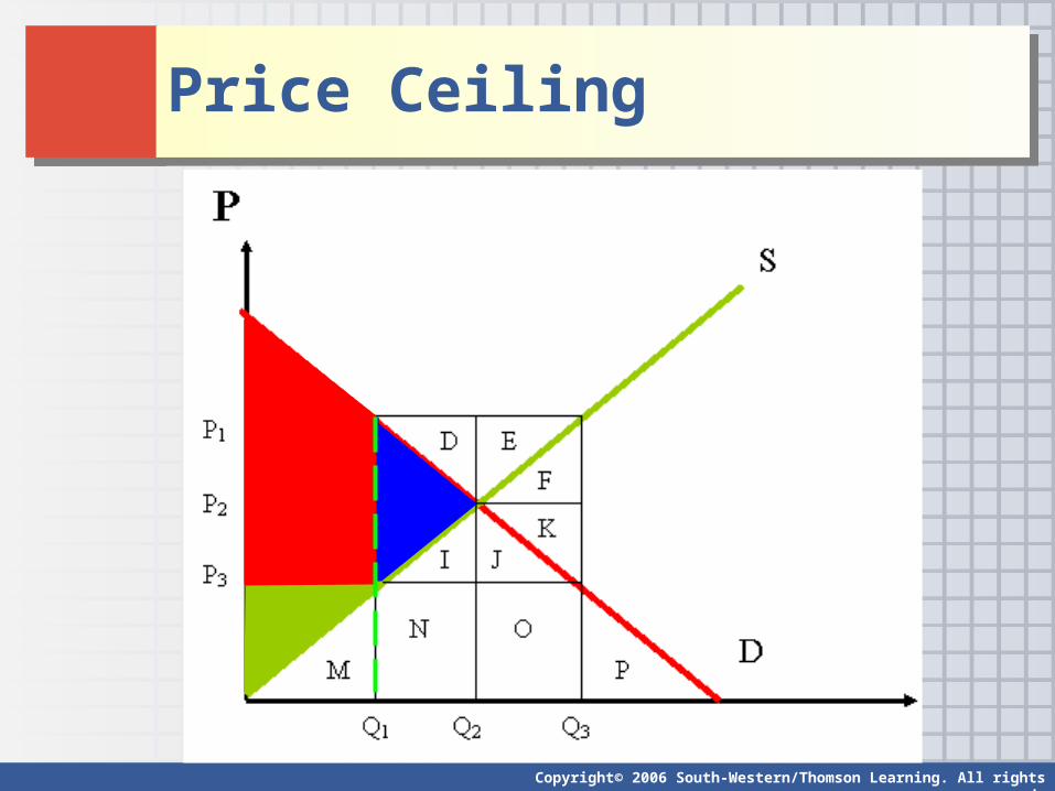
Price CeilingPrice Ceiling
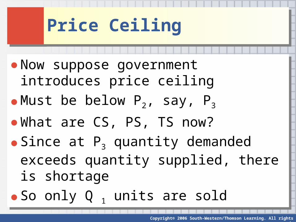
● Now suppose government introduces price ceiling
● Must be below P2, say, P3
● What are CS, PS, TS now?
● Since at P3 quantity demanded exceeds quantity supplied, there is shortage
● So only Q 1 units are sold
● Now suppose government introduces price ceiling
● Must be below P2, say, P3
● What are CS, PS, TS now?
● Since at P3 quantity demanded exceeds quantity supplied, there is shortage
● So only Q 1 units are sold
Copyright© 2006 South-Western/Thomson Learning. All rights reserved.
Price CeilingPrice Ceiling
Copyright© 2006 South-Western/Thomson Learning. All rights reserved.
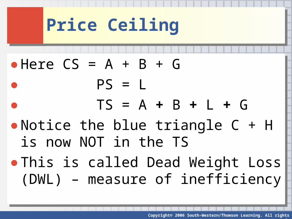
Price CeilingPrice Ceiling
● Here CS = A + B + G
● PS = L
● TS = A + B + L + G
● Notice the blue triangle C + H is now NOT in the TS
● This is called Dead Weight Loss (DWL) – measure of inefficiency
● Here CS = A + B + G
● PS = L
● TS = A + B + L + G
● Notice the blue triangle C + H is now NOT in the TS
● This is called Dead Weight Loss (DWL) – measure of inefficiency
Copyright© 2006 South-Western/Thomson Learning. All rights reserved.
Fighting the Invisible Hand: The Market Fights BackFighting the Invisible Hand: The Market Fights Back
● Restraining the Market Mechanism: Price Ceilings♦ Shortages
♦ Black markets with higher prices
♦ Underinvestment
♦ Vested interests that resist change
● Restraining the Market Mechanism: Price Ceilings♦ Shortages
♦ Black markets with higher prices
♦ Underinvestment
♦ Vested interests that resist change
Copyright© 2006 South-Western/Thomson Learning. All rights reserved.
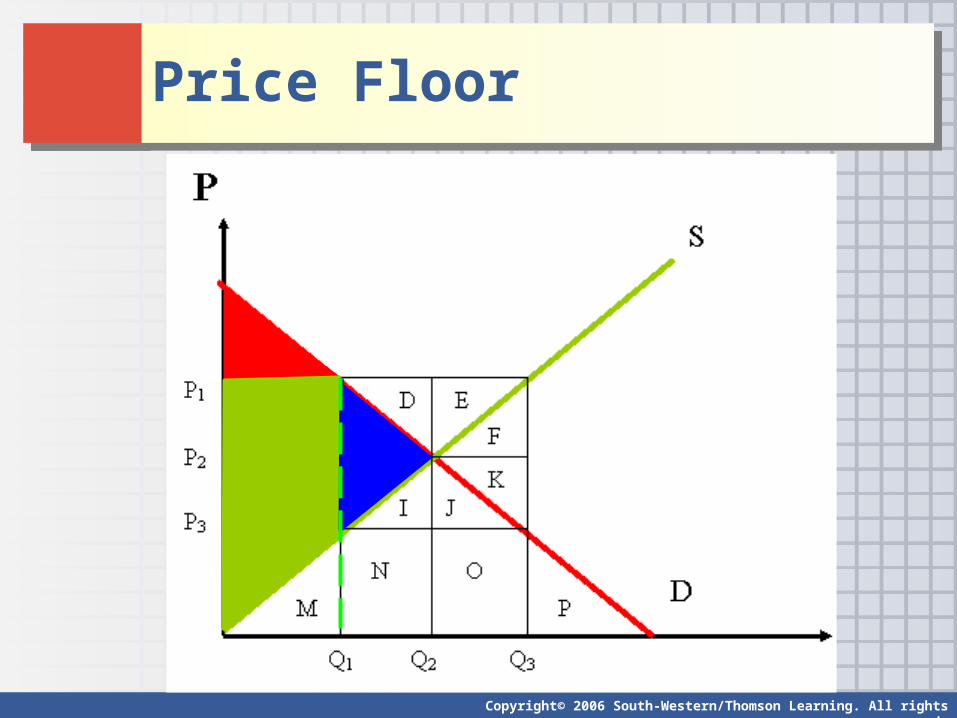
Price FloorPrice Floor
● Now suppose government introduces price floor
● Must be above P2, say, P1
● What are CS, PS, TS now?
● Since at P1 quantity supplied exceeds quantity demanded, there is surplus
● Again only Q1 units are sold
● Now suppose government introduces price floor
● Must be above P2, say, P1
● What are CS, PS, TS now?
● Since at P1 quantity supplied exceeds quantity demanded, there is surplus
● Again only Q1 units are sold
Copyright© 2006 South-Western/Thomson Learning. All rights reserved.
Price FloorPrice Floor
Copyright© 2006 South-Western/Thomson Learning. All rights reserved.
Price FloorPrice Floor
● Here CS = A
● PS = L + B + G
● TS = A + B + L + G
● Notice the blue triangle C + H is now NOT in the TS again
● So we again have DWL from interfering with the market mechanism
● Here CS = A
● PS = L + B + G
● TS = A + B + L + G
● Notice the blue triangle C + H is now NOT in the TS again
● So we again have DWL from interfering with the market mechanism
Copyright© 2006 South-Western/Thomson Learning. All rights reserved.
Fighting the Invisible Hand: The Market Fights BackFighting the Invisible Hand: The Market Fights Back
● Restraining the Market Mechanism: Price Floors♦ Surpluses
♦ Disposal problems
♦ Overinvestment
♦ Vested interests that resist change
● Restraining the Market Mechanism: Price Floors♦ Surpluses
♦ Disposal problems
♦ Overinvestment
♦ Vested interests that resist change
Copyright© 2006 South-Western/Thomson Learning. All rights reserved.
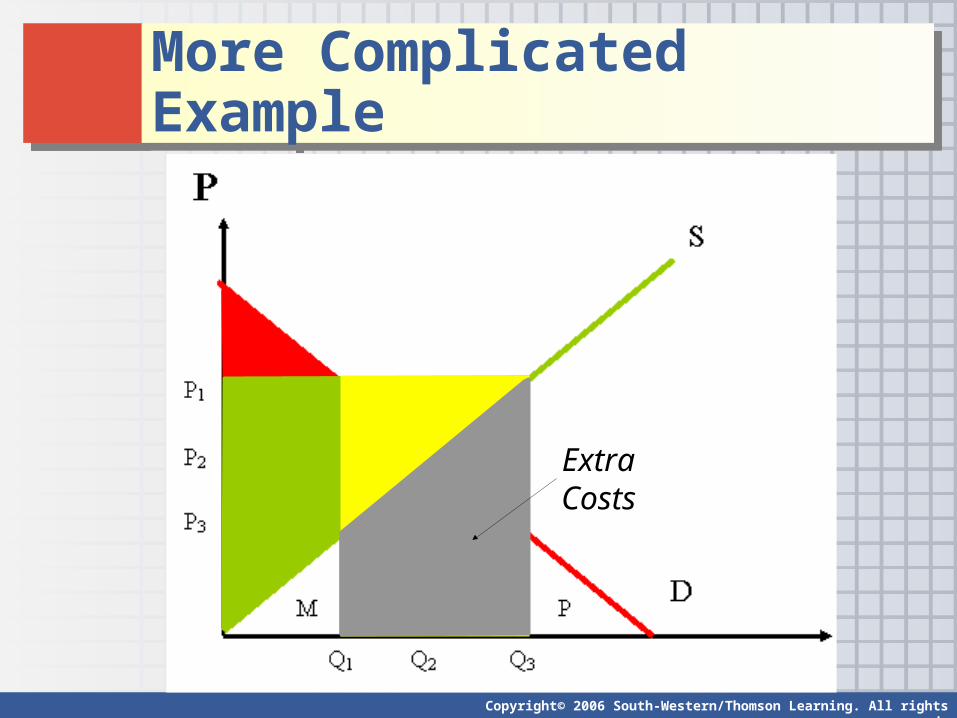
More Complicated ExampleMore Complicated Example
● By simply fixing price we make some group better off at the expense of the other group
● Total result is negative, however
● Maybe government can help?
● Suppose again fix price at P1 as a floor, but government buys all the surplus that consumers do not want to buy
● By simply fixing price we make some group better off at the expense of the other group
● Total result is negative, however
● Maybe government can help?
● Suppose again fix price at P1 as a floor, but government buys all the surplus that consumers do not want to buy
Copyright© 2006 South-Western/Thomson Learning. All rights reserved.
More Complicated ExampleMore Complicated Example
Extra Costs
Copyright© 2006 South-Western/Thomson Learning. All rights reserved.
More Complicated ExampleMore Complicated Example
● Clearly costs of government intervention do not compensate the extra gain for producer
● So intervention is in general not a good idea
● Later on in the course we will see examples when government intervention is beneficial
● Clearly costs of government intervention do not compensate the extra gain for producer
● So intervention is in general not a good idea
● Later on in the course we will see examples when government intervention is beneficial
Copyright© 2006 South-Western/Thomson Learning. All rights reserved.
Tax Policy AnalysisTax Policy Analysis
● Suppose government wants to introduce a tax on producers
● There are many different taxes
● We consider the easiest – per-unit sales tax
● It means that producers have to pay a fixed amount of money to the government for every unit they have sold
● Suppose government wants to introduce a tax on producers
● There are many different taxes
● We consider the easiest – per-unit sales tax
● It means that producers have to pay a fixed amount of money to the government for every unit they have sold
Copyright© 2006 South-Western/Thomson Learning. All rights reserved.
Tax Policy AnalysisTax Policy Analysis
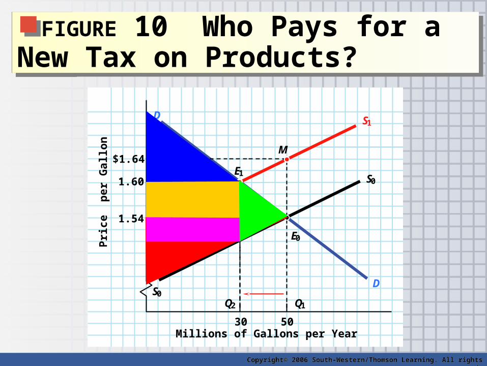
● Costs of producers stay the same
● So they translate tax into price one-for-one♦ Suppose the government introduces a sales tax of 10
cents per gallon of milk♦ This shifts supply curve up♦ How much equilibrium changes is determined by
demand elasticity
● However, all tax burden is split between consumer and producer
Copyright© 2006 South-Western/Thomson Learning. All rights reserved.
FIGURE 10 Who Pays for a New Tax on Products?
FIGURE 10 Who Pays for a New Tax on Products?
Millions of Gallons per Year
Pri
ce p
er G
allo
n
30 50
1.60
1.54
$1.64
Q2 Q1
D
D
S0
S0
S1
S1
M
E0
Copyright© 2006 South-Western/Thomson Learning. All rights reserved.
E1
Copyright© 2006 South-Western/Thomson Learning. All rights reserved.
Tax Policy AnalysisTax Policy Analysis
● Notice that both consumers and producers pay tax, even though government wants to tax producers only
● How tax burden is split between consumers and producers?♦ Depends on price elasticities of supply and
demand
♦ Or, more precise, on the relative elasticity
● Notice that both consumers and producers pay tax, even though government wants to tax producers only
● How tax burden is split between consumers and producers?♦ Depends on price elasticities of supply and
demand
♦ Or, more precise, on the relative elasticity
Copyright© 2006 South-Western/Thomson Learning. All rights reserved.
A Simple But Powerful Lesson A Simple But Powerful Lesson
● Self-interested actions of buyers and sellers laws of supply and demand
● Difficult to resist
● Interference counterproductive effects
● Self-interested actions of buyers and sellers laws of supply and demand
● Difficult to resist
● Interference counterproductive effects
Copyright© 2006 South-Western/Thomson Learning. All rights reserved.
The EndThe End
??????