Embed Size (px)
Citation preview
Topic 2 (a)Demand & Supply
Module 2 Topic 1
Demand & Supply
1. Demand
2. Supply
3. Market Equilibrium
4. Consumer & Producer Surplus
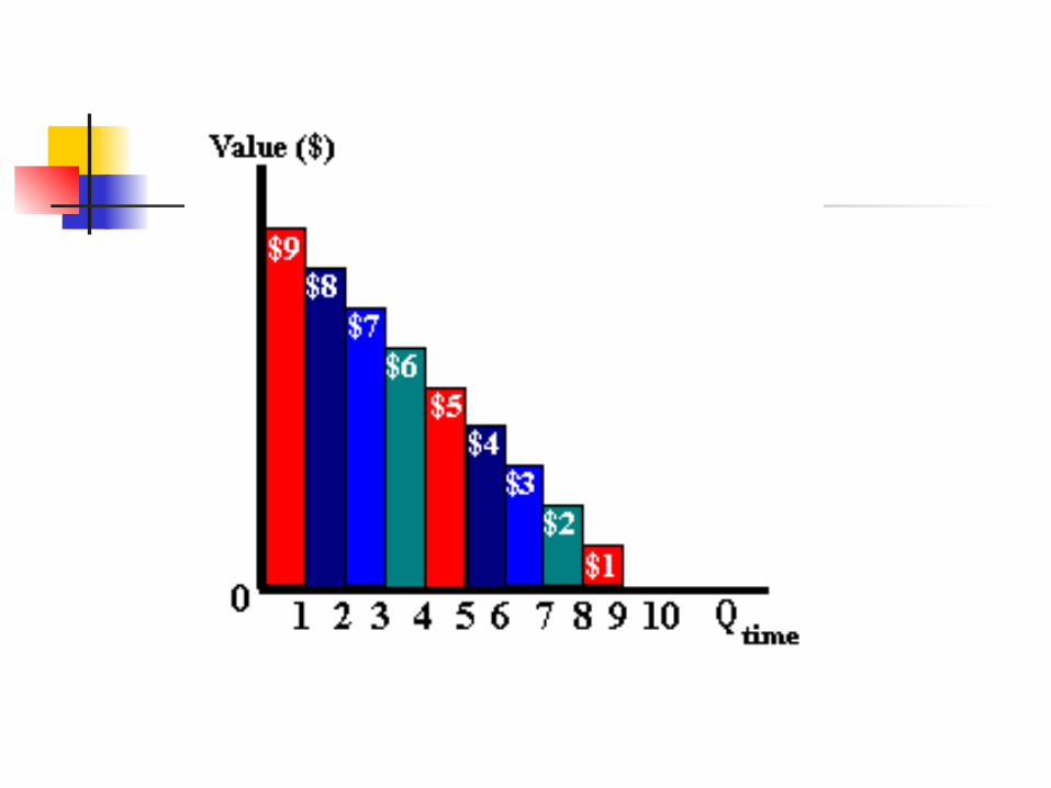
1.1 What is demand?
No. of units of a good or service that consumers are willing and able to purchase during a period, under a given set of conditions

1.2 Why is the study of demand important for firms?
Determines a firm’s profitability Affect long run planning and
strategic decisions Affects short run decisions
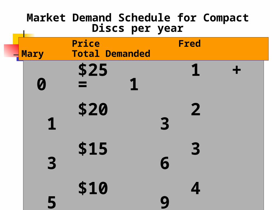
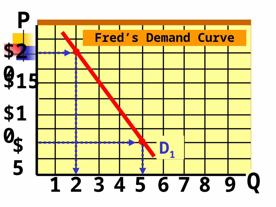
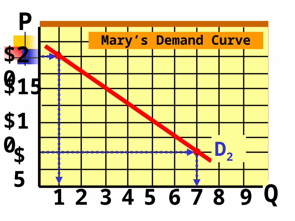
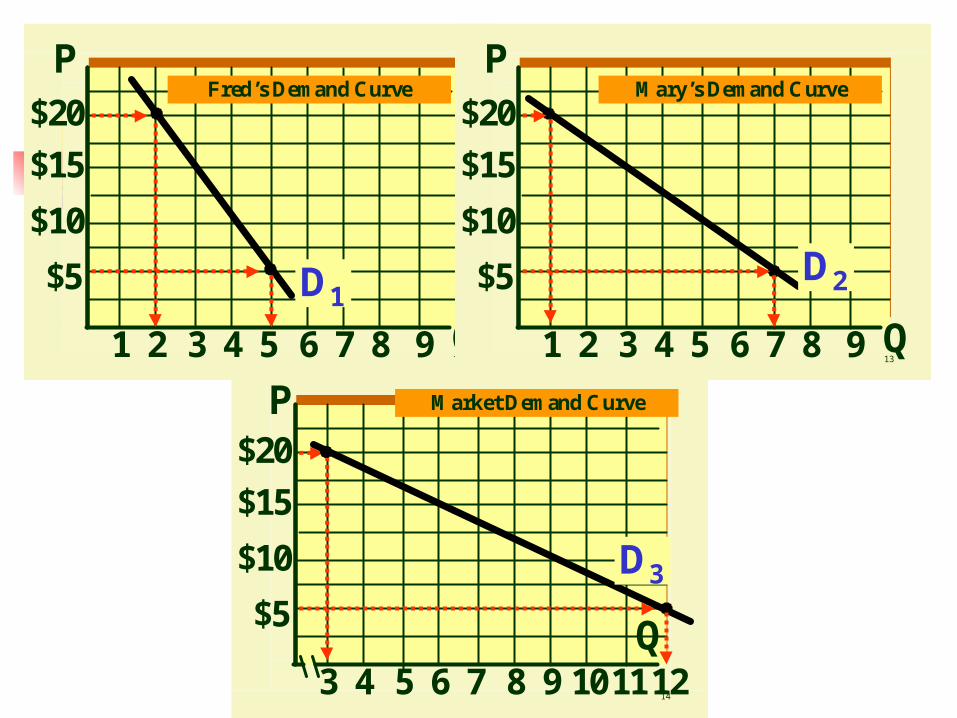
$25 1 + 0 = 1
$20 2 1 3
$15 3 3 6
$10 4 5 9
$5 5 7 12
Price Fred Mary Total Demanded
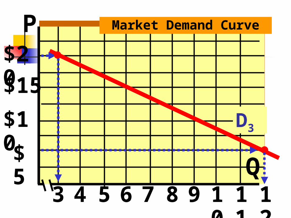
Market Demand Schedule for Compact Discs per year
$20
$15
$10
$5
1 2 3 4
P
Q5 6 7 8 9
Fred’s Demand Curve
D1
$20
$15
$10
$5
1 2 3 4
P
Q5 6 7 8 9
Mary’s Demand Curve
D2
$20
$15
$10
$5
3 4 5 6
P
Q7 8 9 1011
Market Demand Curve
D3
12
12
$20
$15
$10
$5
1 2 3 4
P
Q5 6 7 8 9
Fred’s Demand Curve
D1
13
$20
$15
$10
$5
1 2 3 4
P
Q5 6 7 8 9
Mary’s Demand Curve
D2
14
$20
$15
$10
$5
3 4 5 6
P
Q7 8 9 1011
Market Demand Curve
D3
12
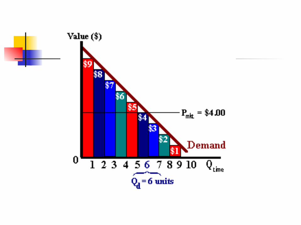
1.3 The Law of demand:
Law of Demand: There is an inverse relationship b/w the
price of a good and the quantity buyers are willing to purchase in a defined time period, other things being the same (ceteris paribus).
When the price of a good rises the quantity demanded will fall and vice versa.
1.3 Law of demand
Reasons for inverse relationship: Income effect: ↑P=> ↓ Real income => ↓ Purchasing power
=> ↓ Qd Substitution effect: ↑P => the good becomes relatively more
expensive => consumers switch to other products => ↓ Qd
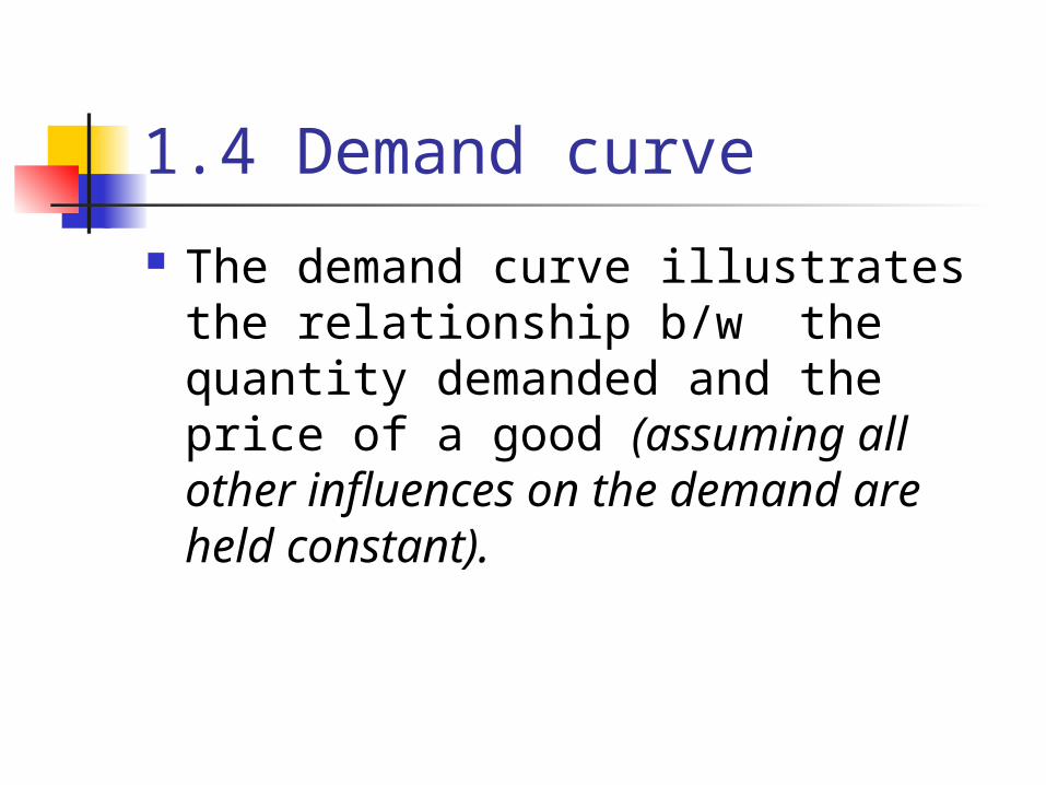
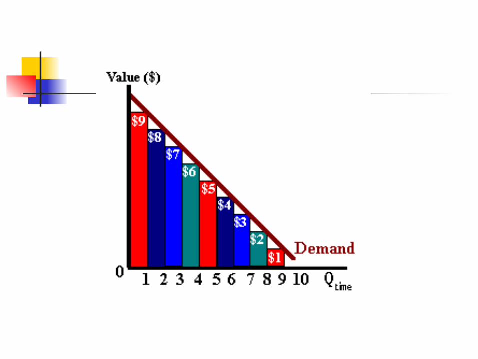
1.4 Demand curve
The demand curve illustrates the relationship b/w the quantity demanded and the price of a good (assuming all other influences on the demand are held constant).

IMPORTANT - KNOW THE DIFFERENCE BETWEEN A CHANGE IN THE QUANTITY DEMANDED AND A CHANGE IN DEMAND
When price changes, what happens?
The curve does not shift - there is a change in the
quantity demanded
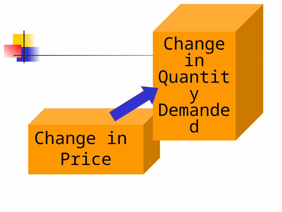
Change in Price
Change in Quantity
Demanded
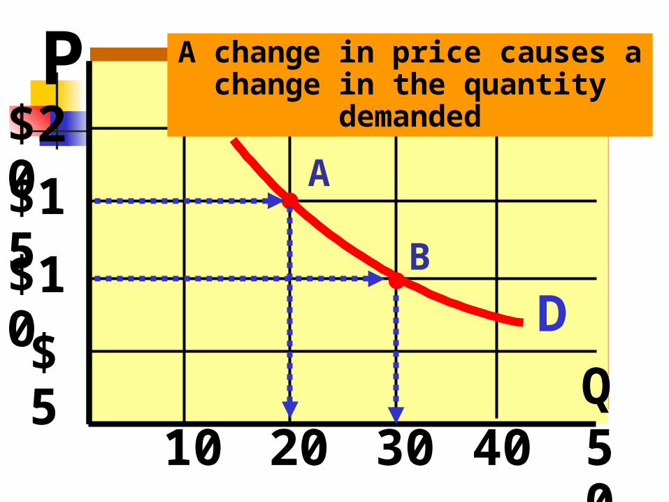
$20
$15
$10
$5
10 20 30 40
A
B
A change in price causes a change in the quantity
demanded
D
P
Q50
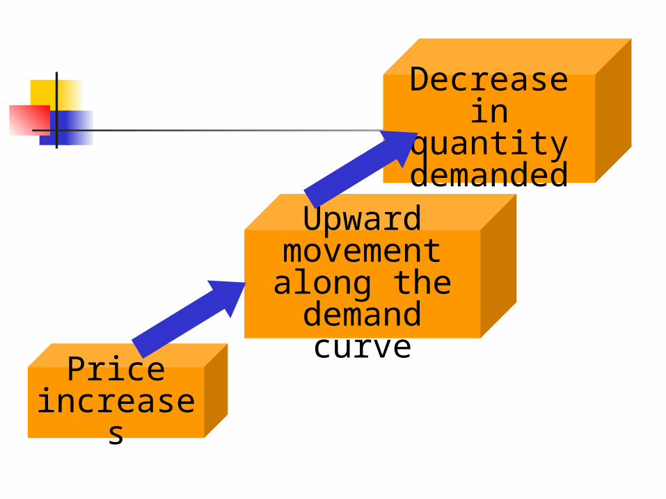
Price increases
Upward movement along the
demand curve
Decrease in quantity
demanded
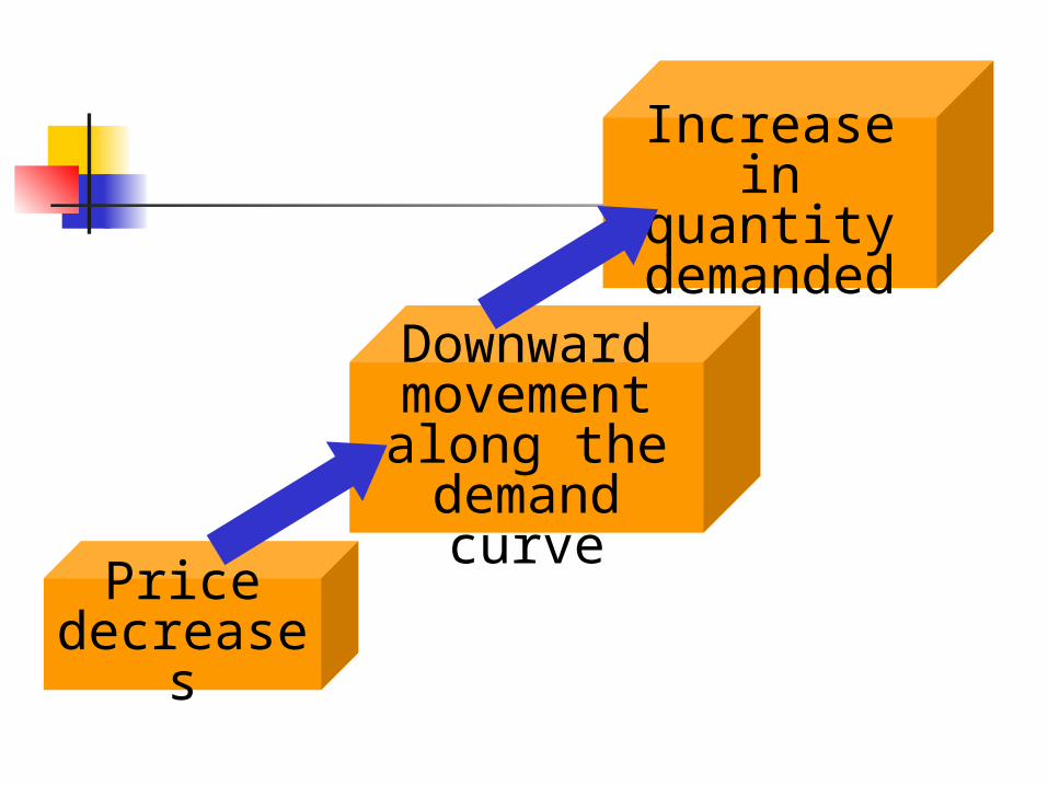
Price decreases
Downward movement along the
demand curve
Increase in quantity
demanded
When something changes other than price, what happens?
The whole curve shifts,there is a
change in demand
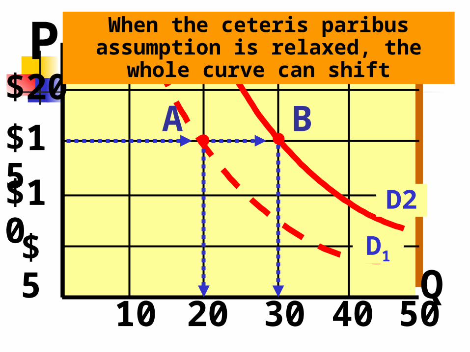
$20
$15
$10
$5
10 20 30 40
D1
D2
P
50
A
When the ceteris paribus assumption is relaxed, the whole curve can shift
Q
B
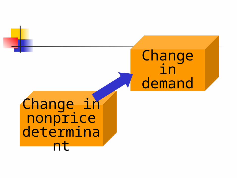
Change innonprice
determinant
Change in demand
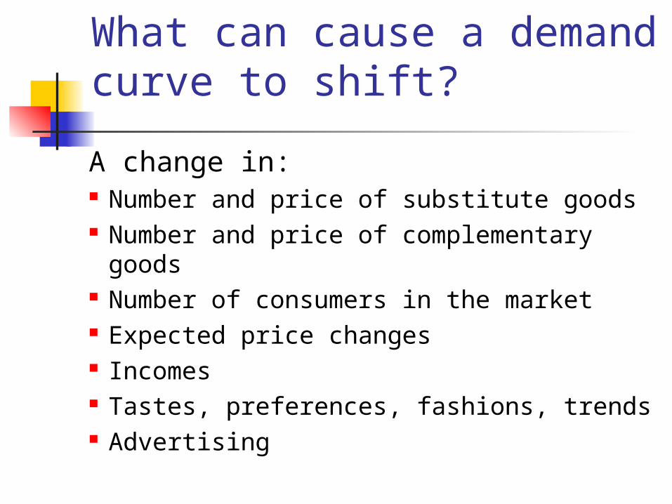
What can cause a demand curve to shift?
A change in: Number and price of substitute goods Number and price of complementary
goods Number of consumers in the market Expected price changes Incomes Tastes, preferences, fashions, trends Advertising
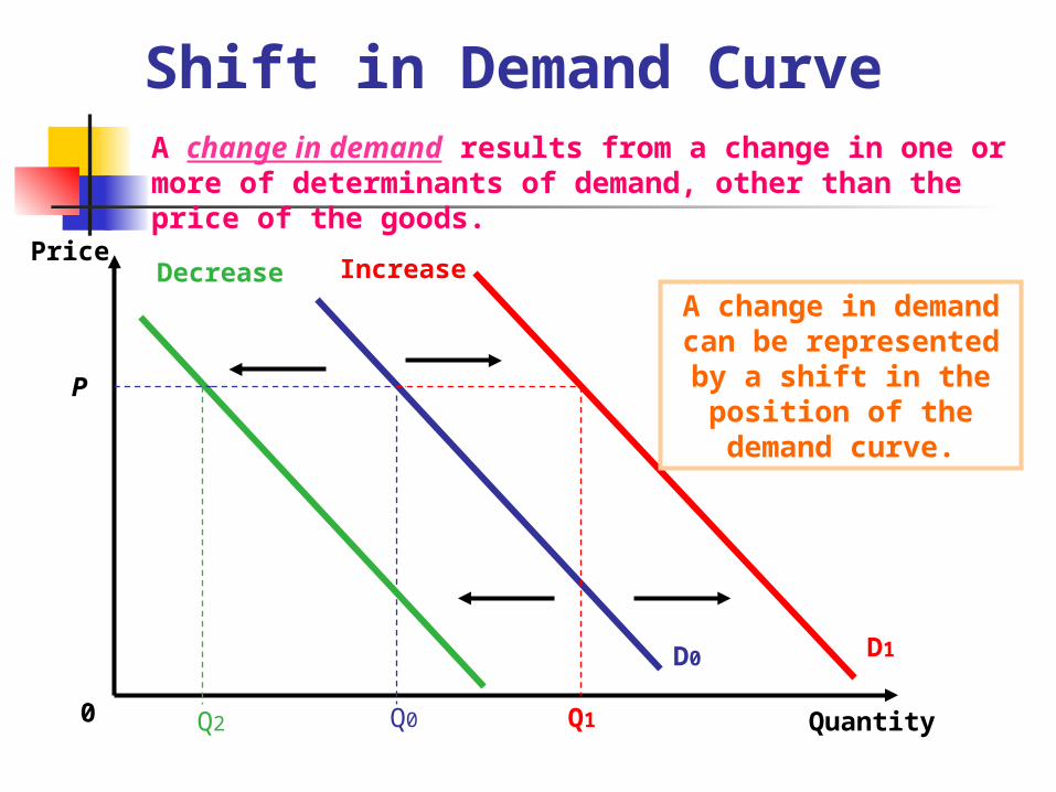
Shift in Demand Curve
P
Price
0 Q0 Q1
D0 D1
QuantityQ2
Decrease Increase
A change in demand results from a change in one or more of determinants of demand, other than the price of the goods.
A change in demand can be represented
by a shift in the position of the demand curve.
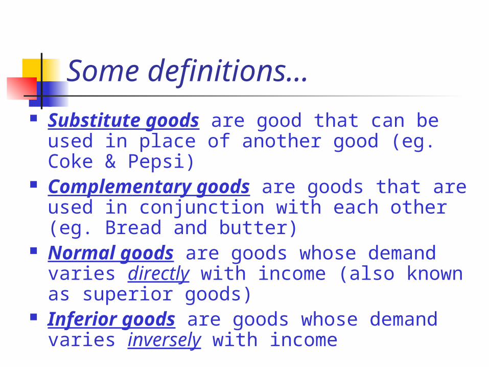
Some definitions… Substitute goods are good that can be
used in place of another good (eg. Coke & Pepsi)
Complementary goods are goods that are used in conjunction with each other (eg. Bread and butter)
Normal goods are goods whose demand varies directly with income (also known as superior goods)
Inferior goods are goods whose demand varies inversely with income
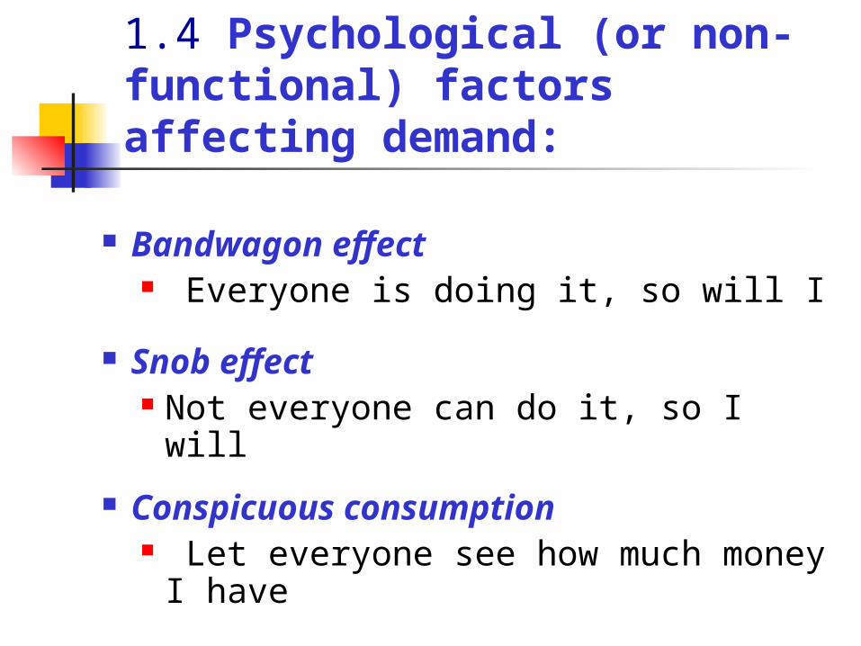
1.4 Psychological (or non-functional) factors affecting demand:
Bandwagon effect Everyone is doing it, so will I
Snob effect Not everyone can do it, so I will
Conspicuous consumption Let everyone see how much
money I have
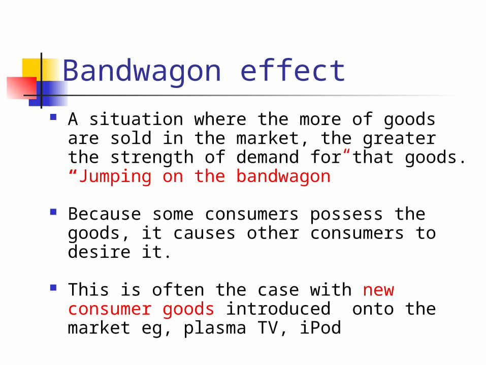
Bandwagon effect A situation where the more of goods are sold
in the market, the greater the strength of demand for that goods. “Jumping on the bandwagon”
Because some consumers possess the goods, it causes other consumers to desire it.
This is often the case with new consumer goods introduced onto the market eg, plasma TV, iPod

Snob effect
Demand for the good strengthens as the availability of that good is reduced.
The scarcity of the good leads consumers to psychologically re-appraise the qualities of the goods.
Eg, Limited Edition Books or Prints; Exclusive Designer Wear
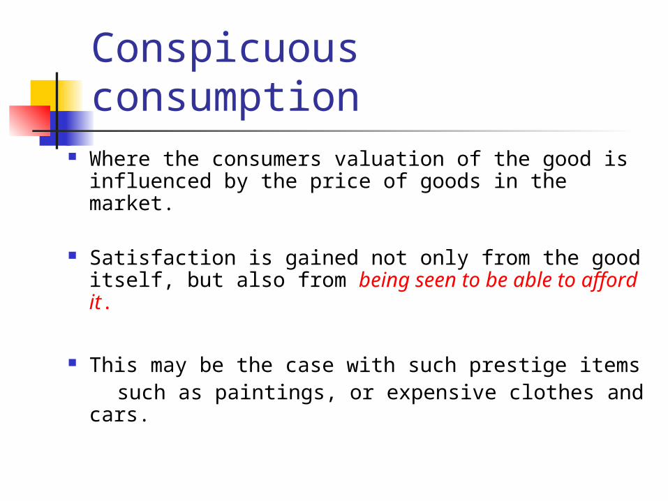
Conspicuous consumption Where the consumers valuation of the good is
influenced by the price of goods in the market.
Satisfaction is gained not only from the good itself, but also from being seen to be able to afford it.
This may be the case with such prestige items such as paintings, or expensive clothes and cars.
2. What is Supply ?
No. of units of a good or service firms are willing and able to produce during a period, under a given set of conditions
2.2 Law of Supply
There is a direct relationship between the price of a good and the quantity sellers are willing to offer for sale in a defined time period, ceteris paribus
2.1 Supply curve
Supply curve: The supply curve shows the
relationship between quantity supplied & price, other things being the same (citeris paribus)

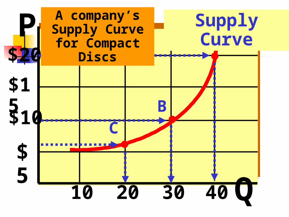
A $20 40
B 10 30
C 6 20
Point Price Quantity
An Individual Seller’s Supply for Compact Discs
$20
$15
$10
$5
10 20 30 40
A
BC
Supply CurveA company’s Supply Curve for Compact Discs
P
Q
Why do supply curves have a positive slope?
A higher price means more profitable to suppliers/sellers.
Therefore, they will supply more of the good or service.
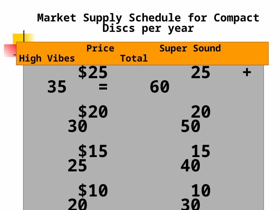
$25 25 + 35 = 60
$20 20 30 50
$15 15 25 40
$10 10 20 30
$5 5 15 20
Price Super Sound High Vibes Total
Market Supply Schedule for Compact Discs per year
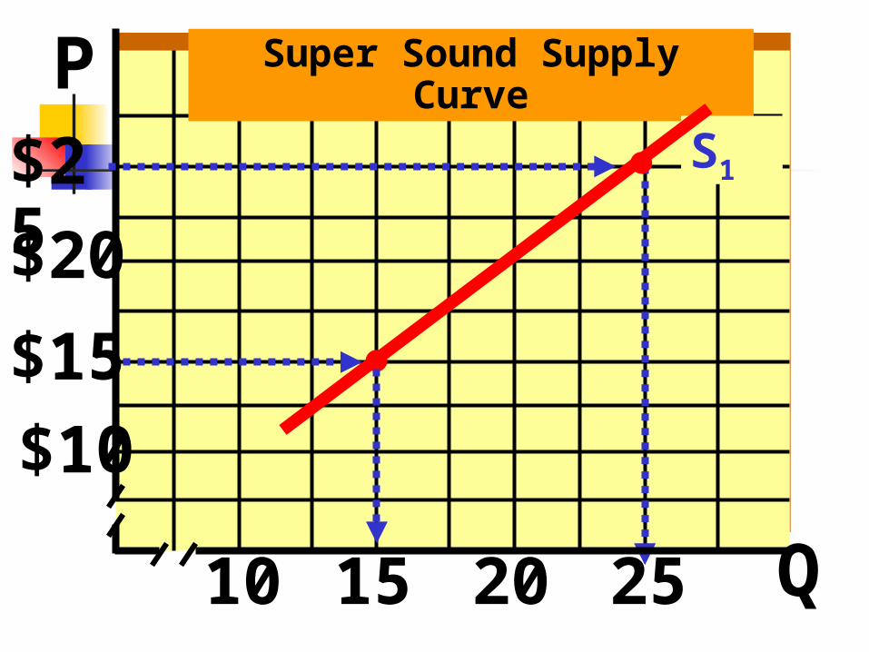
$25
$20
$15
$10
10
P
Q15 20
Super Sound Supply Curve
S1
25
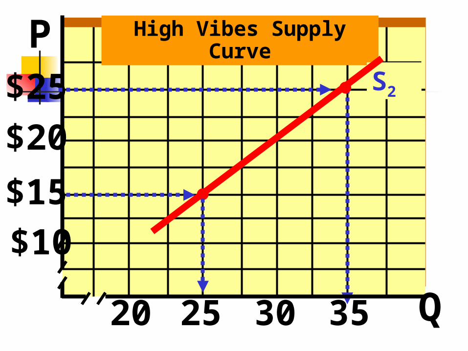
$25
$20
$15
$10
20
P
Q25 30
High Vibes Supply Curve
S2
35
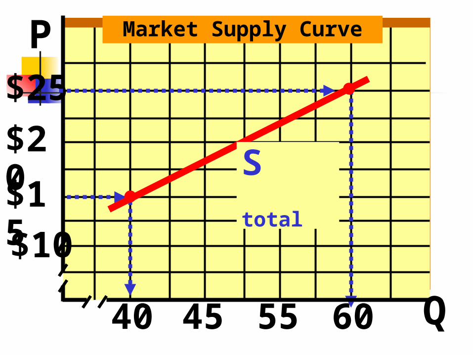
$25
$20
$15
$10
40
P
Q45 55
Market Supply Curve
60
S total
IMPORTANT - KNOW THE DIFFERENCE BETWEEN A CHANGE IN THE QUANTITY SUPPLIED AND A CHANGE IN SUPPLY
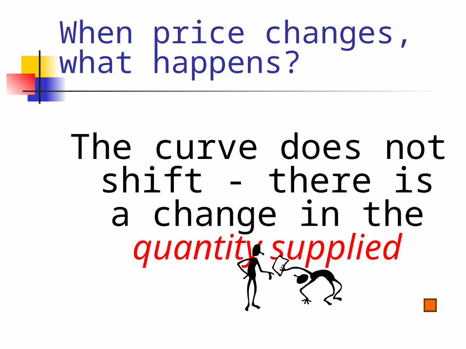
When price changes, what happens?
The curve does not shift - there is a change in the
quantity supplied
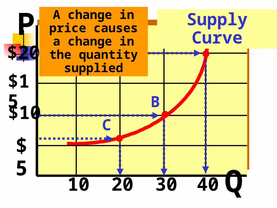
$20
$15
$10
$5
10 20 30 40
A
B
C
Supply CurveA change in price causes a change
in the quantity supplied
P
Q
Change in Price
Change in Quantity Supplied
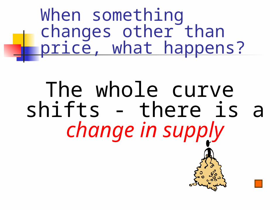
When something changes other than price, what happens?
The whole curve shifts - there is a change in
supply
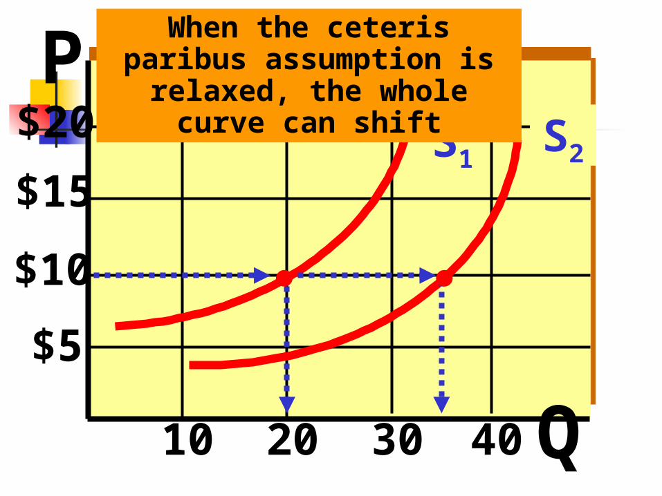
$20
$15
$10
$5
10 20 30 40
S1S2
When the ceteris paribus assumption is relaxed, the
whole curve can shiftP
Q
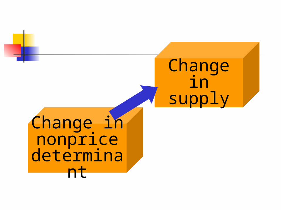
Change innonprice
determinant
Change in supply
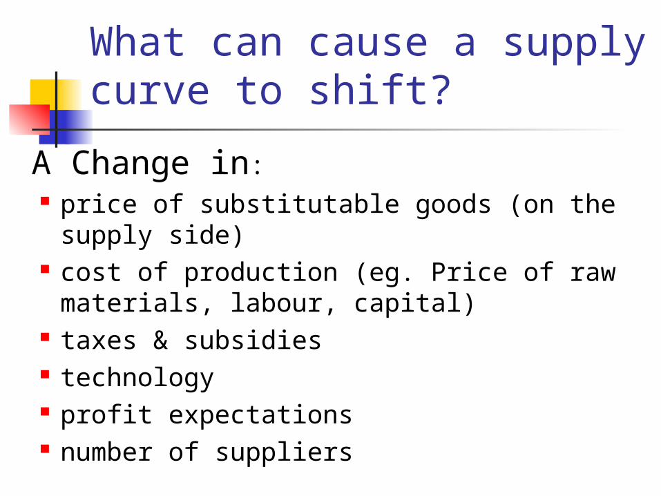
What can cause a supply curve to shift?
A Change in: price of substitutable goods (on the supply
side) cost of production (eg. Price of raw
materials, labour, capital) taxes & subsidies technology profit expectations number of suppliers
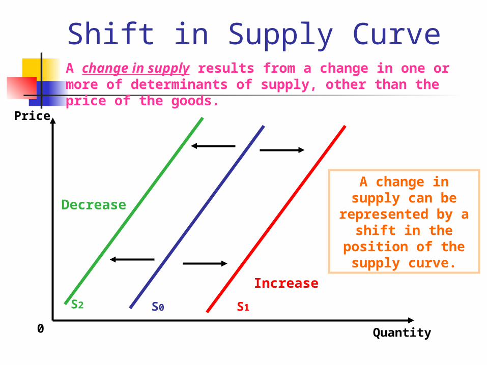
Shift in Supply Curve
Price
0
S0 S1
Quantity
Increase
Decrease
S2
A change in supply results from a change in one or more of determinants of supply, other than the price of the goods.
A change in supply can be
represented by a shift in the
position of the supply curve.
3. Market equilibrium
The point where quantity demanded equals quantity supplied
Market forces keep the price at equilibrium (how?)
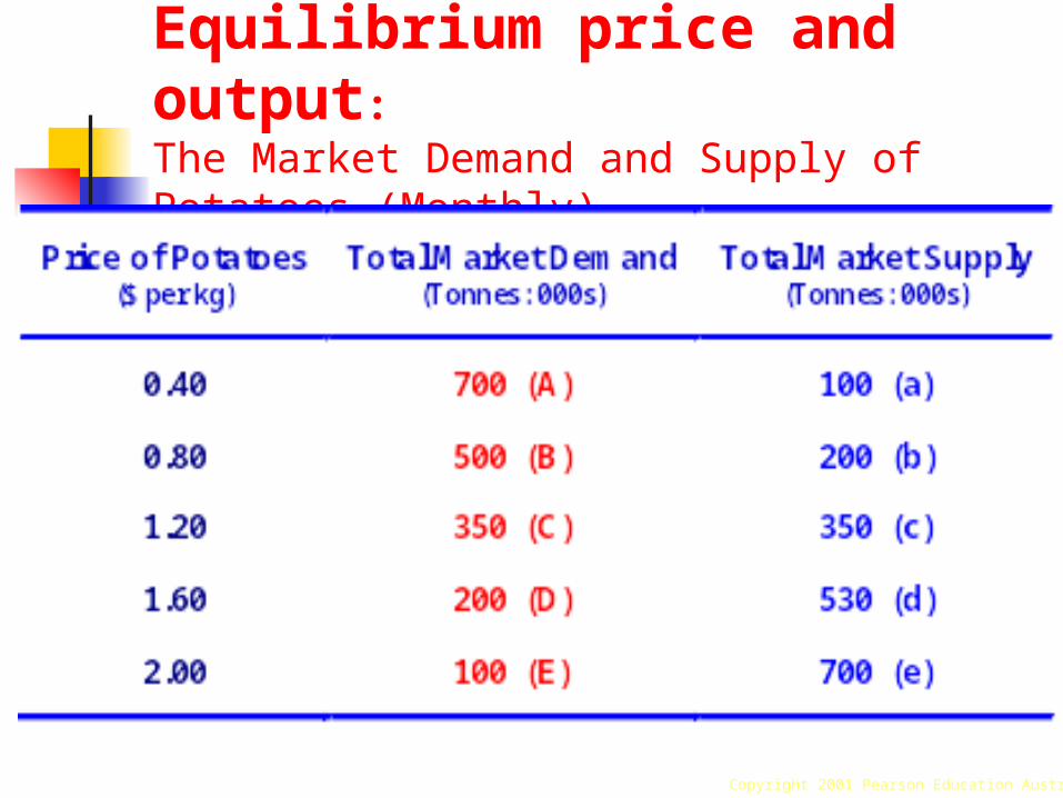
Equilibrium price and output:The Market Demand and Supply of Potatoes (Monthly)
Copyright 2001 Pearson Education Australia
fig
0
0.4
0.8
1.2
1.6
2
0 100 200 300 400 500 600 700 800
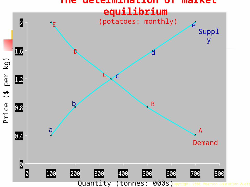
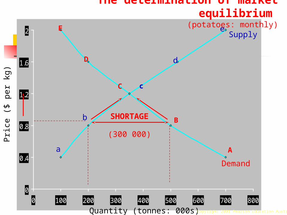
The determination of market equilibrium (potatoes: monthly)
Quantity (tonnes: 000s)
Pri
ce (
$ p
er
kg)
E
D
C
B
Aa
b
c
d
eSupply
Demand
Copyright 2001 Pearson Education Australia
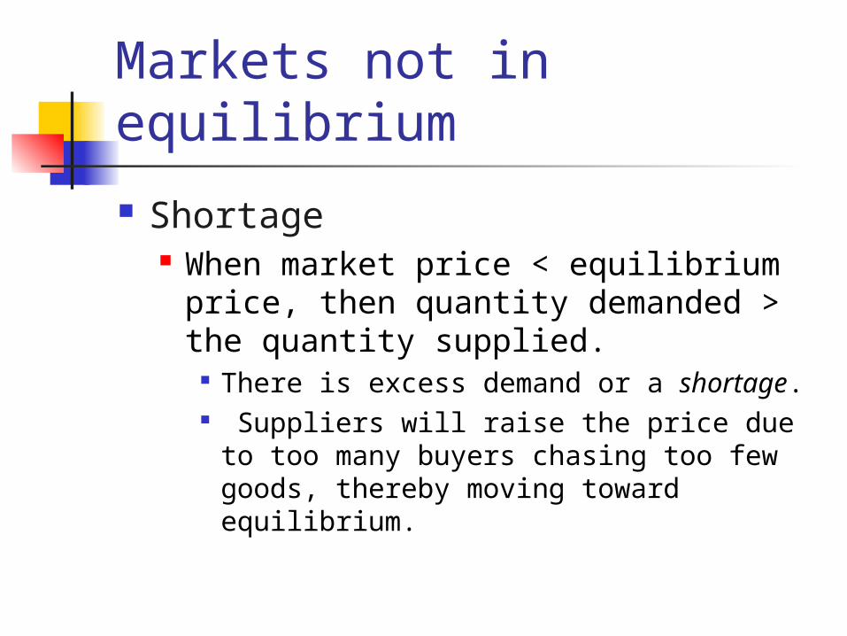
Markets not in equilibrium
Shortage When market price < equilibrium
price, then quantity demanded > the quantity supplied.
There is excess demand or a shortage. Suppliers will raise the price due to too
many buyers chasing too few goods, thereby moving toward equilibrium.
fig
0
0.4
0.8
1.2
1.6
2
0 100 200 300 400 500 600 700 800
Quantity (tonnes: 000s)
Pri
ce (
$ p
er
kg)
E
D
C
B
Aa
b
d
eSupply
Demand
SHORTAGE
(300 000)
The determination of market equilibrium
(potatoes: monthly)
Copyright 2001 Pearson Education Australia
c
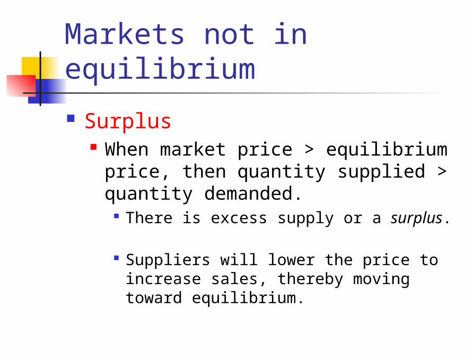
Markets not in equilibrium
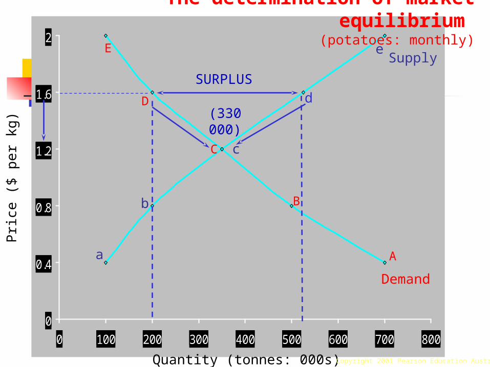
Surplus When market price > equilibrium
price, then quantity supplied > quantity demanded.
There is excess supply or a surplus. Suppliers will lower the price to increase
sales, thereby moving toward equilibrium.
fig
0
0.4
0.8
1.2
1.6
2
0 100 200 300 400 500 600 700 800
Quantity (tonnes: 000s)
Pri
ce (
$ p
er
kg)
E
D
C
B
Aa
b
c
d
e
SURPLUS
(330 000)
Supply
Demand
The determination of market equilibrium
(potatoes: monthly)
Copyright 2001 Pearson Education Australia
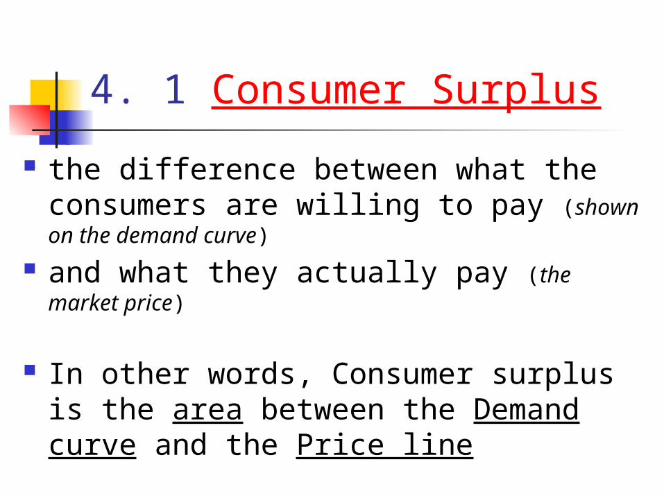
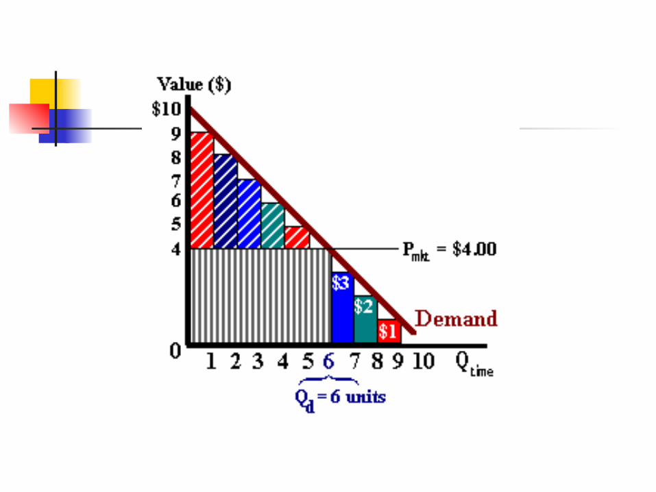
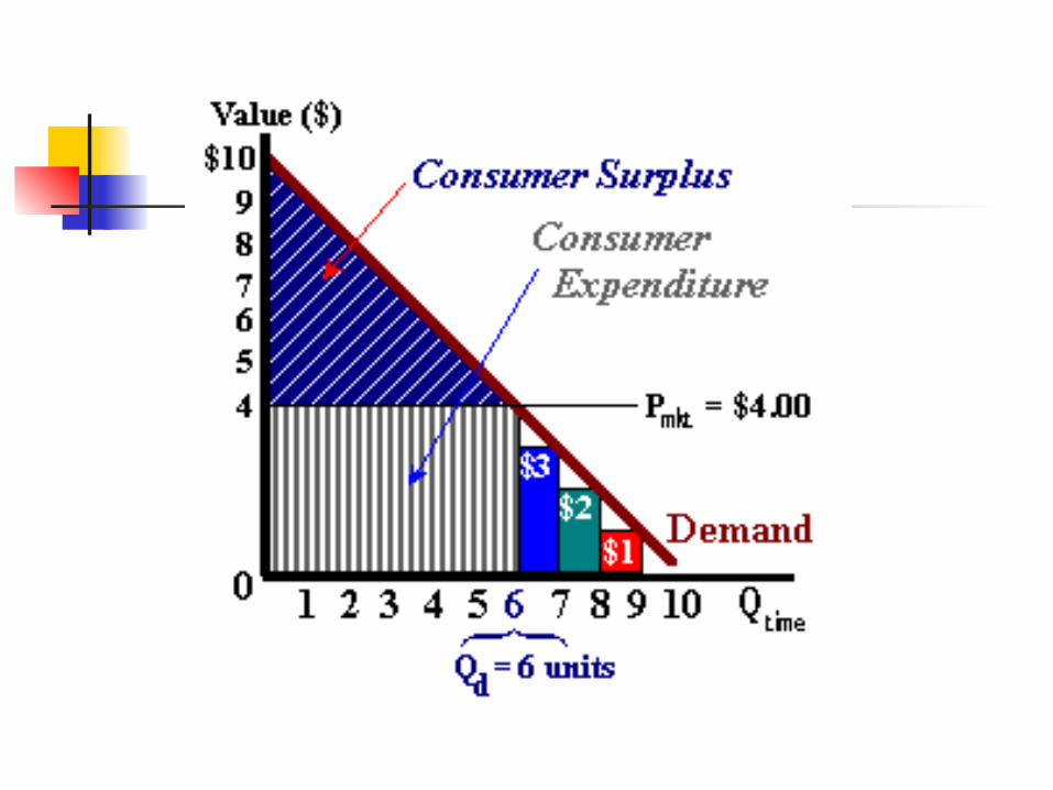
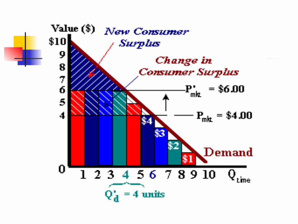
4. 1 Consumer Surplus
the difference between what the consumers are willing to pay (shown on the demand curve)
and what they actually pay (the market price)
In other words, Consumer surplus is the area between the Demand curve and the Price line
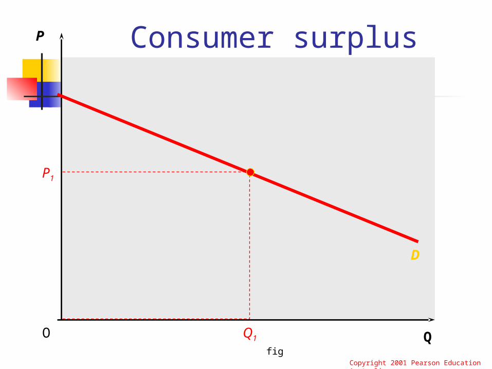
fig
Consumer surplus
D
P1
Q1
P
QO
Copyright 2001 Pearson Education Australia
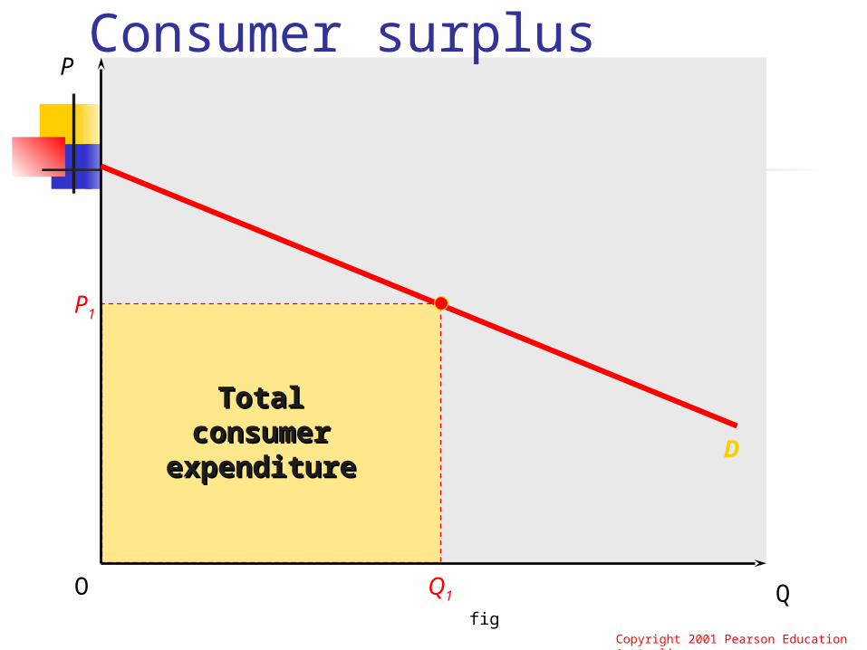
fig
Consumer surplus
D
TotalTotalconsumerconsumer
expenditureexpenditure
P1
Q1
P
QO
Copyright 2001 Pearson Education Australia
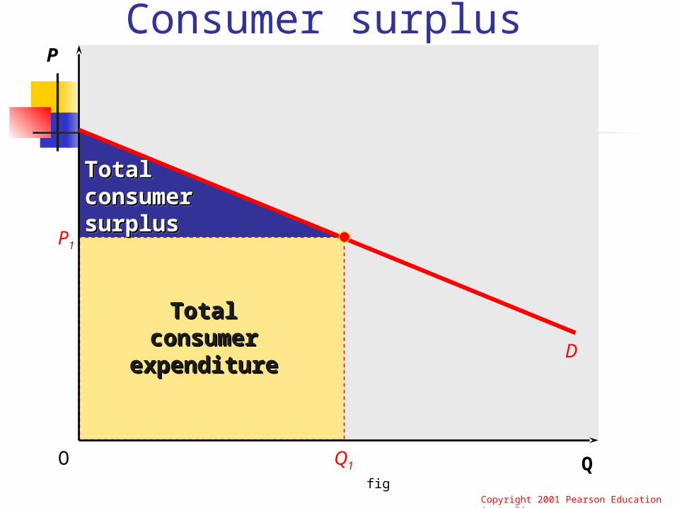
fig
Consumer surplus
D
TotalTotalconsumerconsumer
expenditureexpenditure
TotalTotalconsumerconsumersurplussurplus
TotalTotalconsumerconsumersurplussurplus
P1
Q1
P
QO
Copyright 2001 Pearson Education Australia
Consumer Surplus
CS is the area between the demand curve and the market price line.
It measures how much the consumer gains from buying goods in the market
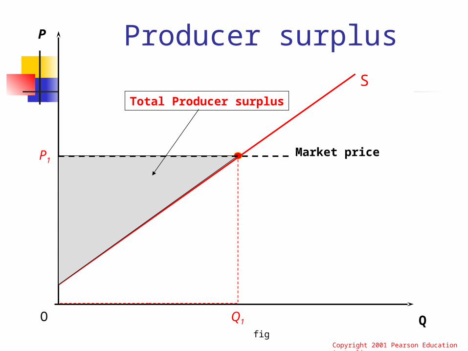
4.2 Producer surplus
the amount producers receive (market price)
above the minimum price required to make them supply the good (shown on the supply curve)
Producer surplus is the area between the Price line and the Supply curve
fig
Producer surplus
P1
Q1
P
QO
Copyright 2001 Pearson Education Australia
S
Producer Surplus
Total Producer surplus
Market price
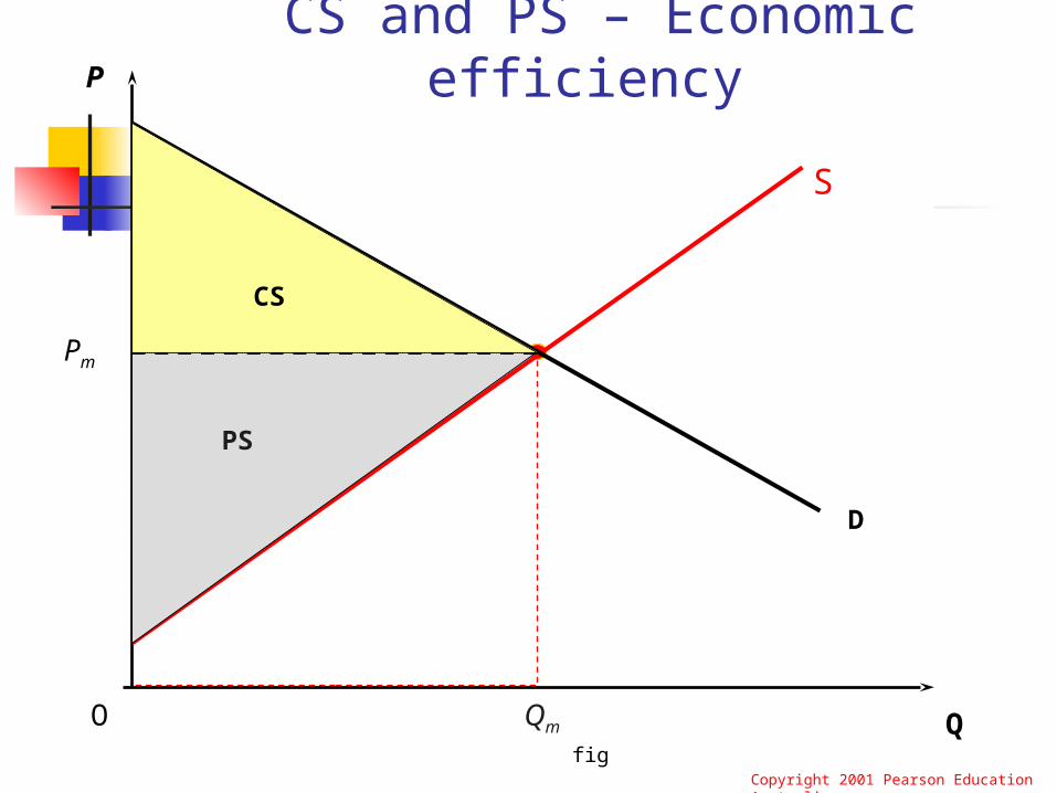
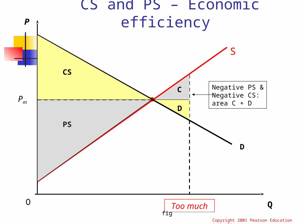
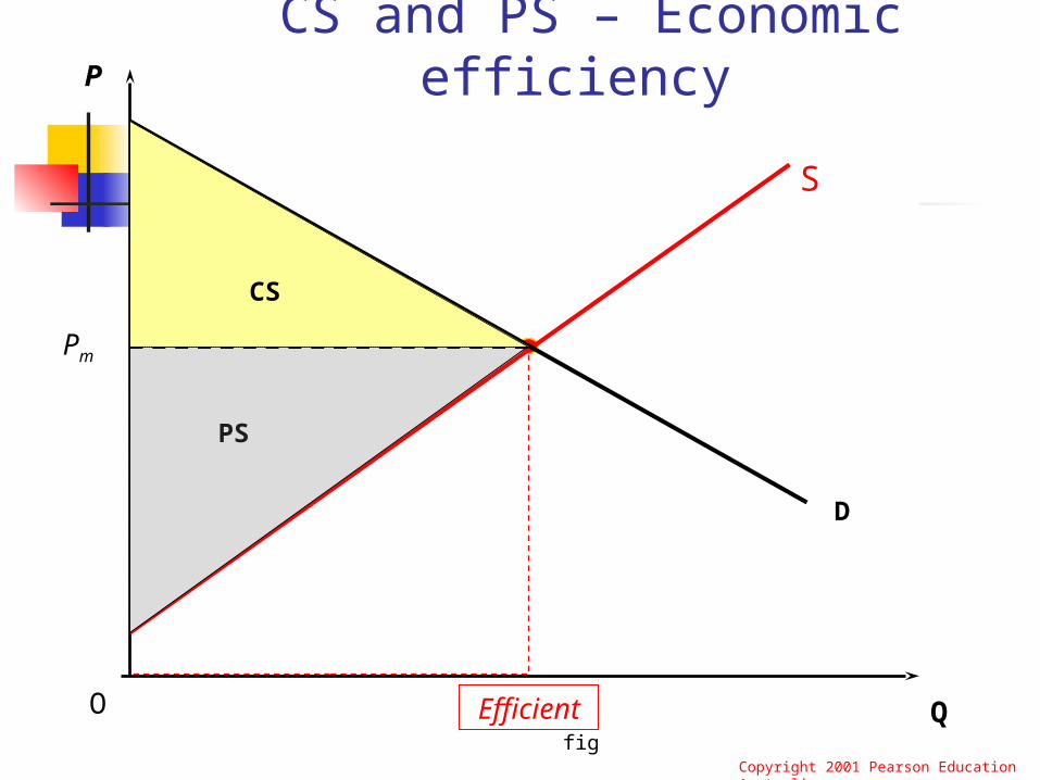
4.3 CS and PS – Economic efficiency
CS and PS are an important tool for measuring the performance of an economic system
or for assessing the impact of alternative government policies in that system.
fig
CS and PS – Economic efficiency
Pm
Qm
P
QO
Copyright 2001 Pearson Education Australia
S
Producer Surplus
PS
CS
D
fig
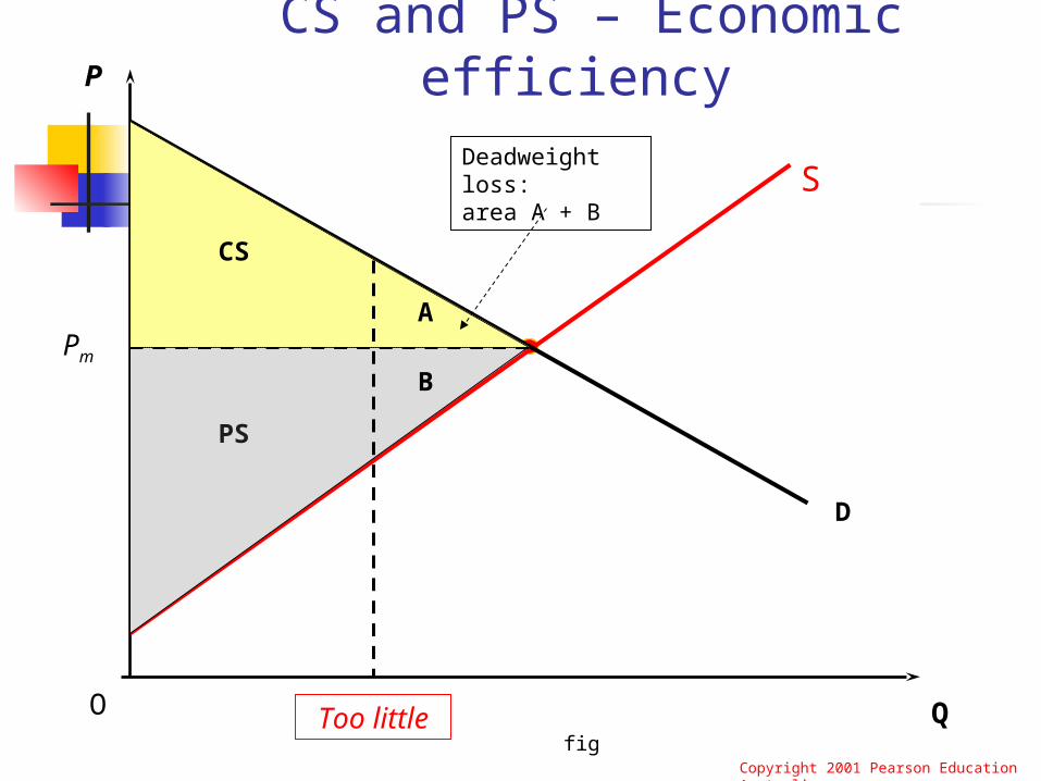
CS and PS – Economic efficiency
Pm
Too little
P
QO
Copyright 2001 Pearson Education Australia
S
Producer Surplus
PS
D
A
B
Deadweight loss:area A + B
CS
fig
CS and PS – Economic efficiency
Pm
Too much
P
QO
Copyright 2001 Pearson Education Australia
S
Producer Surplus
PS
D
CS
C
D
Negative PS &Negative CS:area C + D
fig
CS and PS – Economic efficiency
Pm
Efficient
P
QO
Copyright 2001 Pearson Education Australia
S
Producer Surplus
PS
CS
D