Computer Methods in Applied Mechanics and Engineering€¦ · the components of certain wave-energy converters. ... Computer Methods in Applied Mechanics and Engineering 199 ... Computer

Computer Methods in Applied Mechanics and Engineering 199 (2010) 2085–2098

Contents lists available at ScienceDirect

Computer Methods in Applied Mechanics and Engineering

j ourna l homepage: www.e lsev ie r.com/ locate /cma

Partitioned simulation of the interaction between an elastic structure and freesurface flow

Joris Degroote a, Antonio Souto-Iglesias b, Wim Van Paepegem c, Sebastiaan Annerel a,Peter Bruggeman d, Jan Vierendeels a,⁎a Department of Flow, Heat and Combustion Mechanics, Ghent University, Sint-Pietersnieuwstraat 41, B-9000 Ghent, Belgiumb Naval Architecture Department (ETSIN), Technical University of Madrid (UPM), Avda. Arco de la Victoria s/n, 28040 Madrid, Spainc Department of Materials Science and Engineering, Ghent University, Sint-Pietersnieuwstraat 41, B-9000 Ghent, Belgiumd Department of Applied Physics, Eindhoven University of Technology, P.O.-Box 513, 5600 MB Eindhoven, The Netherlands

⁎ Corresponding author.E-mail addresses: [email protected] (J. Degro

(A. Souto-Iglesias), [email protected] (W. [email protected] (S. Annerel), [email protected] (J. Vierendeels).

URL's: http://www.FSI.UGent.be/ (J. Degroote), http(W. Van Paepegem).

0045-7825/$ – see front matter © 2010 Elsevier B.V. Aldoi:10.1016/j.cma.2010.02.019

a b s t r a c t
a r t i c l e i n f o
Article history:Received 12 October 2009Received in revised form 12 February 2010Accepted 18 February 2010Available online 25 March 2010

Keywords:Fluid–structure interactionPartitionedFree surfaceVolume-of-fluidRolling tankImpactIQN-ILSAitken relaxation

Currently, the interaction between free surface flow and an elastic structure is simulated with monolithiccodes which calculate the deformation of the structure and the liquid–gas flow simultaneously. In this work,this interaction is calculated in a partitioned way with a separate flow solver and a separate structural solverusing the interface quasi-Newton algorithm with approximation for the inverse of the Jacobian from a least-squares model (IQN-ILS). The interaction between an elastic beam and a sloshing liquid in a rolling tank iscalculated and the results agree well with experimental data. Subsequently, the impact of both a rigidcylinder and a flexible composite cylinder on a water surface is simulated to assess the effect of slamming onthe components of certain wave-energy converters. The impact pressure on the bottom of the rigid cylinderis nearly twice as high as on the flexible cylinder, which emphasizes the need for fluid–structure interactioncalculations in the design process of these wave-energy converters. For both the rolling tank simulations andthe impact simulations, grid refinement is performed and the IQN-ILS algorithm requires the same number ofiterations on each grid. The simulations on the coarse grid are also executed using Gauss-Seidel couplingiterations with Aitken relaxation which requires significantly more coupling iterations per time step.

ote), [email protected] Paepegem),[email protected] (P. Bruggeman),

://www.composites.UGent.be/

l rights reserved.

© 2010 Elsevier B.V. All rights reserved.

1. Introduction

Over the past decade, the simulation of fluid–structure interaction(FSI) has gained interest, resulting in numerous biomedical [1–3] andengineering [4,5] applications. More recently, the level of complexityof FSI simulations has increased by the addition of advanced modelssuch as free surface flow to the coupled problem [6–10]. Multiphaseflow can be highly unsteady because of waves and droplets. Theinteraction between such an unsteady flow and a structure can changeabruptly due to impact of a structure on a free surface or a wavehitting an already deforming structure. This strong time dependencecauses additional difficulties in FSI simulations.

Free surface flowhas since long fascinated scientists and engineers,possibly due to the countless spectacular applications, and severalnumerical methods have been devised. Most of these methods can be

categorized as interface-tracking, interface-capturing or particlemethods. Interface-tracking methods represent the liquid–gas inter-face by means of a chain of grid nodes in 2D or a surface in 3D. Thesegrid nodes move at the same speed as the fluids over a static [11] ordeforming [12,13] fluid grid. Interface-capturing methods use a gridwhich does not deform due to themotion of the fluid and some kind ofmarkerwhich is transportedwith the flow to determine onwhich sideof the liquid–gas interface a cell is located. The Volume-Of-Fluid (VOF)method employs a marker variable to store the fraction of the cell thatis filled with a given phase [14,15] and the Level Set method indicatesthe liquid–gas interface with the zero level of a smooth function [16].The Particle Finite Element Method (PFEM) [17] and SmoothedParticle Hydrodynamics (SPH) [18] are particle methods but alsolatticemethods [19] fit in this category. Several benchmarks have beenestablished to compare and verify all these simulation techniques, forexample the well-known dam-break problem [20].

FSI and coupled problems in general can be simulated in either amonolithic or a partitioned way. In the monolithic approach, theequations of the subproblems are solved simultaneously, therebytaking into account the interaction between the subproblems duringthe solution process. This results in a large system of generallynonlinear coupled equations which is often solved with Newtoniterations [21] with suitable preconditioning for the different blocks in

mailto:[email protected]






http://www.FSI.UGent.be/

http://www.composites.UGent.be/

http://dx.doi.org/10.1016/j.cma.2010.02.019

http://www.sciencedirect.com/science/journal/00457825

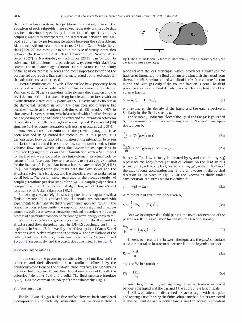
Fig. 1. The fluid subdomain Ωf, the solid subdomain Ωs, their boundaries Γf and Γs andthe fluid–structure interface Γi.

2086 J. Degroote et al. / Computer Methods in Applied Mechanics and Engineering 199 (2010) 2085–2098

the resulting linear systems. In a partitioned simulation, however, theequations of each subproblem are solved separately with a code thathas been developed specifically for that kind of equations [22]. Acoupling algorithm incorporates the interaction between the sub-problems, often by performing iterations between the subproblems.Algorithms without coupling iterations [23] and Gauss-Seidel itera-tions [1,24,25] are mostly unstable in the case of strong interactionbetween the flow and the structure. However, quasi-Newton itera-tions [26,27] or Newton-Krylov techniques [28,29] can be used tosolve such FSI problems in a partitioned way, even with black-boxsolvers. The main advantage of monolithic simulations is the stabilityof the solution process, whereas the most important benefit of thepartitioned approach is that existing, mature and optimized codes forthe subproblems can be reused.

Several simulations of FSI with a free surface have previously beenperformed with considerable attention for experimental validation.Walhorn et al. [6] use a space-time finite element discretization and theLevel Set method to simulate a rising bubble and dam-break with anelastic obstacle. Antoci et al. [7] work with SPH to calculate a variation ofthe dam-break problem in which the dam does not disappear butbecomes flexible at the bottom. Idelsohn et al. [8,9] employ PFEM tosimulate various cases, amongwhichdam-breakwith aflexible obstacle, asolidobject impactingandfloatingonwaterand the interactionbetweenaflexible structure and the sloshingflow in a rolling tank. Potapov et al. [10]simulate fluid–structure interaction with tearing structures using SPH.

However, all results mentioned in the previous paragraph havebeen obtained using monolithic techniques. In this paper, it isdemonstrated how partitioned simulation of the interaction betweenan elastic structure and free surface flow can be performed. A finitevolume flow code which solves the Navier-Stokes equations inarbitrary Lagrangian-Eulerian (ALE) formulation with a VOF modelfor the free surface is coupled with a finite element structural code bymeans of interface quasi-Newton iterations using an approximationfor the inverse of the Jacobian from a least-squares model (IQN-ILS)[27]. This coupling technique treats both the flow solver and thestructural solver as a black box and the algorithm will be explained indetail below. The performance (measured as the average number ofcoupling iterations per time step) of the IQN-ILS coupling algorithm iscompared with another partitioned algorithm, namely Gauss-Seideliterations with Aitken relaxation [30,31].

An existing case, namely the sloshing flow in a rolling tank with aflexible obstacle [9], is simulated and the results are compared withexperiments to demonstrate that the partitioned approach results in thecorrect solution. Subsequently, the impact of both a rigid and a flexiblecomposite cylinderonawater surface is simulated toaccelerate thedesignprocess of a particular component for floating wave-energy converters.

Section 2 describes the governing equations for the flow and thestructure and their discretization. The IQN-ILS coupling algorithm isexplained in Section 3, followed by a brief description of Gauss-Seideliterations with Aitken relaxation in Section 4. The simulations of therolling tank and falling cylinder are presented in Section 5 andSection 6, respectively, and the conclusions are listed in Section 7.

2. Governing equations

In this section, the governing equations for the fluid flow and thestructure and their discretization are outlined, followed by theequilibriumconditionson thefluid–structure interface. The subdomainsare indicated as Ωf and Ωs and their boundaries as Γf and Γs, with thesubscript f denoting fluid and s solid. The fluid–structure interfaceΓi=Γf∩Γs is the common boundary of these subdomains (Fig. 1).

2.1. Flow equations

The liquid and the gas in the free surface flow are both consideredincompressible and mutually immiscible. This multiphase flow is

modeled with the VOF technique, which introduces a scalar volumefraction αf throughout the fluid domain to distinguish the liquid fromthe gas [14,15]. A region is filled with liquid only if the volume fractionis one and with gas only if the volume fraction is zero. The fluidproperties such as the fluid density ρf are written as a function of thevolume fraction

ρf = αf ρl + ð1−αf Þρg ð1Þ

with ρl and ρg the density of the liquid and the gas, respectively.Similarly for the fluid viscosity μf.

The unsteady, isothermal flow of the liquid and the gas is governedby the conservation of mass and a single set of Navier-Stokes equa-tions, given by

∂ρf∂t + ∇⋅ ρf vf

� �= 0 ð2aÞ

∂ρf vf∂t + ∇⋅ ρf vf vf

� �−∇⋅τf = f f ð2bÞ

for xaΩf. The flow velocity is denoted by vf and the time by t. ffrepresents the body forces per unit of volume on the fluid. In thispaper, gravity is the only body force so ff=−ρf g1y with g=9.81m/s2

the gravitational acceleration and 1y the unit vector in the verticaldirection as indicated in Fig. 1. For the Newtonian fluids underconsideration, the stress tensor is defined as

τf = −pI + 2μγ ð3aÞ

with the rate of strain tensor γ given by

γ =12

∇vf + ð∇vf ÞTh i

: ð3bÞ

For two incompressible fluid phases, the mass conservation of thephases results in an equation for the volume fraction, namely

∂αf

∂t + ∇⋅ αf vf� �

= 0: ð4Þ

There is nomass transfer between the liquid and thegas. Also, surfacetension is not taken into account because both the Reynolds number

Re =ρlvlLμl

ð5aÞ

and the Weber number

We =ρlvlLσlg

ð5bÞ

aremuch larger than one, withσlg being the surface tension coefficientbetween the liquid and the gas and L the appropriate length scale.

The flow equations are discretized in space on a grid with triangularand rectangular cells using the finite volumemethod. Scalars are storedin the cell centres and a power law is used to obtain momentum

2087J. Degroote et al. / Computer Methods in Applied Mechanics and Engineering 199 (2010) 2085–2098

variables at the faces. Gradients at the cell centres are calculated fromthe face values using the Green-Gauss theorem. The face values for thegradient calculations are the arithmetic average of the node values,which are in turn theweighted average of the values in the cells aroundthe node. The pressure interpolation at the faces is performed with astaggered grid approach similar to the one described by Patankar [32].Eqs. (2) are solved using the Pressure-Implicit with Splitting ofOperators (PISO) scheme with skewness and neighbour correction.Algebraic multigrid is employed to accelerate the convergence.

The grid of the fluid domain is deforming, driven by the defor-mation of the fluid–structure interface. Smoothing with fictitioussprings between the grid nodes is applied for deformations during thetime step. Cells which have either become too skewed or which falloutside the range of desired cell sizes are eliminated once in each timestep. The implicit backward Euler time discretization of Eqs. (2) in ALEformulation is first order accurate on a moving grid.

Eq. (4) for the volume fraction is solved with first order explicittime discretization but the time step for this equation is only a fractionof the time step of the FSI calculation such that the Courant numberdoes not exceed 0.25 near the liquid–gas interface. However, thevolume fraction is recalculated after each grid deformation and theconvective flux coefficients are updated based on the new volumefractions. The liquid–gas interface is reconstructed with a piecewise-linear approach for an accurate calculation of the fluxes through thefaces near the liquid–gas interface [33].

2.2. Structural equations

The deformation ds of the structure is determined by the conser-vation of momentum

ρs∂2ds

∂t2−∇⋅σs = f s ð6Þ

for xaΩswith ρs the structural density and fs=−ρsg1y the body forceper unit volume on the structure. The relation between the stresstensor σs and the strain tensor

�s =12

∇ds + ∇dsð ÞTh i

ð7Þ

is given by the constitutive equation of the material, in this case alinear-elastic material law.

σs = C : �s: ð8Þ

The value of C depends on the material and will therefore bedifferent for the test cases presented in Section 5 and Section 6, wherethis and other case-dependent assumptions will be documented.

The structure is discretized with finite elements. Geometricnonlinearity is taken into account during the solution process and thestress on the fluid–structure interface follows the rotation of thestructure during the time step. Unconditionally stable implicit Hilber-Hughes-Taylor time integration [34] is used with a small numericaldamping parameter αs=−0.05.

2.3. Equilibrium conditions

The equilibrium conditions on the fluid–structure interface are thekinematic condition

vf =∂ds

∂t ð9Þ

and the dynamic condition

nf ⋅σf = −ns⋅σs ð10Þ

for xaΓi with d the displacement, σ the stress tensor and n the unitnormal vector that points outwards from the domainΩ. The Dirichlet-Neumann formulation of the FSI problem is employed, which meansthat the flow equations are solved for a given velocity of the fluid–structure interface, whereas a stress is imposed on the fluid–structureboundary of the solid domain. The time discretization converts Eq. (9)into equality of the displacements on the fluid–structure interface.Appropriate conditions such as no-slip walls and constant pressureboundaries are imposed on Γf nΓi and displacements or rotations areapplied on ΓsnΓi.

As the fluid and solid have a different discretization on the fluid–structure interface, an interpolation has to be performed. To transferthe displacement from the solid side to the fluid side of the interface,the fluid grid nodes are projected orthogonally on the boundaryof the structural grid, after which the displacement at the location ofthis projection is calculated with linear interpolation of the valuesat the two nearest structural nodes. The stresses on the solidside of the fluid–structure interface are obtained in an analogousway from the stresses on the fluid side by orthogonal projection ofthe load integration points on the fluid grid followed by linearinterpolation. Although other interpolation techniques exist [35,36],this simple approach is chosen because it does not require anyinformation about the connectivity or discretization in the solvers,which is consistent with the black-box approach of the IQN-ILScoupling algorithm and the Gauss-Seidel iterations with Aitkenrelaxation. The interpolation will be hidden in the following sectionsto avoid additional notation.

3. Interface quasi-Newton coupling algorithm

In this section, the flow solver and the structural solver areredefined as functions with the degrees-of-freedom on the interfaceas input and output. These functions will subsequently be used in theexplanation of the coupling algorithms. In the remainder of this paper,all values and functions are at the new time level n+1, unlessindicated otherwise with a superscript n. A right superscript kindicates the coupling iteration within time step n+1 and a subscriptdenotes the element in a vector. Capital letters denote matrices, boldlower case letters and lower case letters represent vectors and scalars,respectively.

The displacement degrees-of-freedom of all nodes on the fluid–structure interface are grouped in a vector daℝu and the normalstress components σ⋅n on all faces of the interface are gathered in avector taℝw. The function

t = FðdÞ ð11Þ

is referred to as the flow solver and it concisely represents severaloperations. The displacement of the fluid–structure interface is passedon to the flow code and the grid of the fluid domain adjacent to theinterface is adapted accordingly. Subsequently, the grid velocity iscalculated and the flow equations are solved for the fluid state in theentire fluid domain, which also results in a stress distribution on theinterface.

The structural solver is represented by the function

d = SðtÞ: ð12Þ

This expression indicates that the stress distribution on theinterface is given to the structural code which then calculates thedisplacement of the entire structure and thus also the newdisplacement of the fluid–structure interface. It is important to noticethat F and S both solve a problem in a subdomain while their inputand output is limited to the fluid–structure interface. Operations ond and t are therefore fast compared to evaluations of these functions.


The equilibrium conditions in Section 2.3 have to be satisfied ineach time step of the FSI simulations so Eqs. (11) and (12) have to besatisfied by the same vector d and t. Elimination of t results in a set ofequations for the displacement vector only

S ∘FðdÞ = d ð13Þ

which is subsequently reformulatedas anonlinear root-findingproblemin the interface's displacement

rðdÞ = S∘FðdÞ−d = 0: ð14Þ

The dependence of r on d is further often omitted for clarity. Thisnonlinear equation in d is solved with quasi-Newton iterations

d̂rdd j

dkΔdk = −rk ð15aÞ

dk+1 = dk + Δdk ð15bÞ

and a hat is used to indicate the approximation of the Jacobian.This approximation is necessary because the exact Jacobian of r(d) isunknown as the Jacobians of the black-box functions F and S areunavailable. In each quasi-Newton iteration, the residual vector iscalculated as the output of the structural solver (d ̃k+1)minus the inputof the flow solver (dk)

rk = rðdkÞ = S ∘FðdkÞ−dk = d̃k +1−dk

: ð16Þ

A tilde indicates that the displacement has been calculated by thestructural solver to distinguish it from the displacement given to theflow solver. Since the displacement calculated by S is only an inter-mediate value that is not used in the next coupling iteration, the tildeis dropped once the displacement for the next iteration has beencalculated.

If the Jacobian dr/dd is approximated and quasi-Newton iterationsare performed, black-box solvers can be used. However, the linearsystem Eq. (15a) with as dimension the number of degrees-of-freedom in the interface's displacement has to be solved in each quasi-Newton iteration. Although the number of degrees-of-freedom in theinterface's displacement is generally smaller than the number ofdegrees-of-freedom in the entire fluid and structure domain, theJacobian matrix dr/dd is usually dense. As a result, the solution of thelinear system Eq. (15a) corresponds to a significant computationalcost in large simulations, especially if a direct solver is used. It istherefore more advantageous to approximate the inverse of theJacobian by applying the least-squares technique introduced by [26]on a particular set of vectors, as will be explained below. Thistechnique can also be used to solve linear systems as demonstrated in[37].

By approximating the inverse of the Jacobian, the quasi-Newtoniterations Eqs. (15a) and (15b) can be written as

dk+1 = dk +d̂rdd j

dk

� �−1

−rk� �

: ð17Þ

It can be seen from Eq. (17) that the approximation for theinverse of the Jacobian does not have to be created explicitly; aprocedure to calculate the product of this matrix with the vector −rk

is sufficient. The vector −rk is the difference between the desired

residual, i.e. 0, and the current residual rk and it is further denotedas Δr=0−rk. The correction of the displacement in Eq. (17) isrewritten as

Δdk =ˆdrdd

� �−1−rk

� �≈ d̂d

dr−rk

� �ð18Þ

with a slight abuse of notation. After substitution of the definition ofthe residual r= d̃−d, this becomes

Δdk≈ d̂ddr

−rk� �

ð19aÞ

=ˆdd̃dr

−I

0@

1A −rk� �

ð19bÞ

=ˆdd̃dr

−rk� �

+ rk: ð19cÞ

Eq. (19c) indicates that the change Δd̃ of the structural solver'soutput due to a given change of the residual Δr=−rk

Δd̃ =ˆdd̃dr

⋅ −rk� �

ð20Þ

has to be approximated. This is done with data obtained during theprevious quasi-Newton iterations: Eq. (16) shows that the flow equa-tions and structural equations are solved in quasi-Newton iteration k,resulting in d̃

k+1= S ∘FðdkÞ and the corresponding residual rk. To

predict how d̃ changeswhen r changes, these vectors are converted intodifferences with respect to the first quasi-Newton iteration.

Δrk = rk−r0 ð21aÞ

Δd̃k+1

= d̃k+1−d̃

1: ð21bÞ

Each quasi-Newton iteration generates an additional vectorΔr andthe corresponding vector Δd̃. These vectors are stored as the columnsof the matrices

Vk = Δrk−1 Δrk−2… Δr1 Δr0

h ið22aÞ

and

Wk = Δ d̃k

Δd̃k−1

… Δd̃2

Δd̃1

h i: ð22bÞ

The number of columns in Vk and Wk is indicated as v and it isgenerally much smaller than the number of rows u. Nevertheless, insimulations with a low number of degrees-of-freedom on the inter-face, it is possible that the number of columns has to be limited to u bydiscarding the rightmost columns.

The desired change of the residualΔr=0−rk is approximated as alinear combination of the known Δri

Δr≈Vkck ð23Þ

with ckaℝv the coefficients of the decomposition. Because v≤u,Eq. (23) is an overdetermined set of equations for the elements of ck

and hence the least-squares solution to this linear system is calculated.Therefore, the so-called economy size QR-decomposition of Vk iscalculated using Householder transformations [38]

Vk = Q kRk ð24Þ


with Qkaℝu×v an orthogonal matrix and Rkaℝv×v an upper triangularmatrix. The coefficient vector ck is then determined by solving thetriangular system

Rkck = Q kTΔr ð25Þ

using back substitution. If aΔr i vector is (almost) a linear combinationof otherΔr j vectors, one of the diagonal elements ofRkwill (almost) bezero. Consequently, the equation corresponding to that row of Rk

cannot be solved during the back substitution. If a small diagonalelement is detected, the corresponding column in Vk is removed andthe QR-decomposition (Eq. (24)) and the solution of the triangularsystem (Eq. (25)) are repeated until none of the diagonal elements istoo small. The tolerance for the detection of small diagonal elementsdepends on how accurately the flow equations and structural equa-tions are solved.

The Δ d̃ that corresponds to Δr≈Vkck can be approximated usingthe same decomposition coefficients ck butwith respect toWk becausethere is a one-to-one relation between the columns of Vk and Wk.Consequently, the Δd̃ sought after in Eq. (20) is given by

Δd̃ = Wkck: ð26Þ

Substitution of Eq. (26) in Eq. (19c) yields

Δd = Wkck + rk: ð27Þ

The complete IQN-ILS technique is shown in the algorithm below.Because thematrices Vk andWk have to contain at least one column, arelaxation with factor ω (line 36) is performed in the second couplingiteration of each time step. The quasi-Newton iterations start from theinitial guess

dn+1;0 =52dn−2dn−1 +

12dn−2 ð28Þ

which is an extrapolation based on the previous time steps. Lowerorder extrapolations are used for the first two time steps. The it-erations in the time step have converged when ||rk||2≤ �o with �o theconvergence tolerance.

The relation between Δr and Δd is thus found by means of the Δd̃values. One might try to relate the residual r directly to d instead ofto d̃, but this obviously will not work as the new input for S ∘F wouldbe a linear combination of the previous inputs. The only newinformation in the input of S ∘F would originate from numericalerrors and consequently the coupling iterations would not converge.More details can be found in [27].

Algorithm 1. IQN-ILS method

1: k=0

2: d̃1=S ∘F(d0)

3: r0= d̃1=d0

4: while ||rk||2 N �0 do

5: if k=0 then

6: dk+1=dk+ωrk

7: else

8: construct Vk and Wk as shown in Eqs. (21a) and (21b) and Eqs.(22a) and (22b)

9: calculate QR-decomposition Vk=QkRk

10: solve Rkck=−QkTrk

11: dk+1=dk+Wkck+rk

12: end if

13: k=k+1

14: d k̃+1=S ∘F(dk)

15: rk= d̃k+1−dk

16: end while

4. Gauss-Seidel iterations with Aitken relaxation

If the interaction between the fluid and the structure is strongthen Gauss-Seidel iterations between the flow solver and the struc-tural solver diverge quickly without any relaxation. However, it isdifficult to determine a priori a value for the relaxation factor whichwill result in fast convergence of the Gauss-Seidel iterations. Aitkenrelaxation [30,31] signifies that a dynamically varying scalarrelaxation factor ωk is used for the Gauss-Seidel iterations within atime step. The next displacement of the fluid–structure interface iscalculated as

dk +1 = dk + ωkrk ð29aÞ

= 1−ωk� �

dk + ωk d̃k +1 ð29bÞ

and consequently the next input for S ∘F is a linear combination of thelast output and the previous input. Moreover, the update of theinterface's position is in the direction of the residual vector, as opposedto the update from the IQN-ILS method. The first relaxation in a timestep is executedwith the relaxation factor from the end of the previoustime step, but limited to ωmax, so ω0=sign(ωn)min(|ωn|,ωmax). Thevalue of ωk is obtained as

ωk = −ωk−1rk−1

� �Trk−rk−1

� �

rk−rk−1� �T rk−rk−1

� � : ð30Þ

5. Rolling tank

The rolling tank cases presented by [9] are simulated to verifythe coupling code and both solvers. These cases consist of arectangular container partially filled with oil or water. This fluidinteracts with a flexible structure which is clamped to either thetop or bottom of the tank. The container rotates around the mid-point of its bottom and a harmonic rolling motion is imposed byan electric motor. Three different configurations are considered,namely a standing beam immersed in shallow oil (Fig. 3), a standingbeam immersed in deep oil (Fig. 4) and a hanging beam aboveshallow water (Fig. 5).

For this rolling tank, data from experiments and two-dimensionalmonolithic PFEM calculations are available [9]. The experiments havebeen performed with a transparent tank such that images could betaken. The displacement of the tip of the beam in the rotatingreference frame of the tank has been calculated from these imageswith a computer programme. Special attention has been paid to thegaps between the flexible structure and the front and back of the tanksuch that the experiments can be considered two-dimensional.


Algorithm 2. Gauss-Seidel iterations with Aitken relaxation [30,31]

1: k=0

2: d̃=S ∘F(d0)

3: r0=d̃−d0

4: while ||rk||2 N �0 do

5: if k=0 then

6: ω0=sign(ωn)min(|ωn|,ωmax)

7: else

8: ωk = −ωk−1 ðrk−1ÞT ðrk−rk−1Þ‖rk−rk−1‖2

9: end if

10: dk+1=dk+ωkrk

11: k=k+1

12: d̃k+1=S ∘F(dk)

13: rk= d̃k+1–dk

14: end while

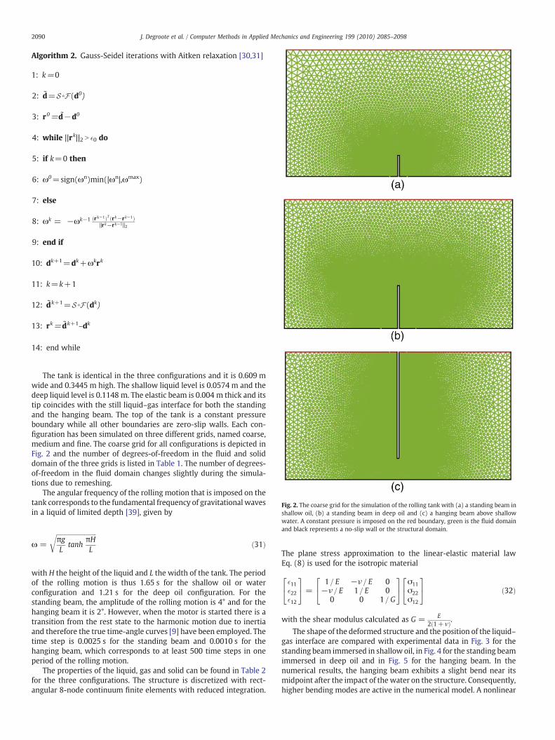
Fig. 2. The coarse grid for the simulation of the rolling tank with (a) a standing beam inshallow oil, (b) a standing beam in deep oil and (c) a hanging beam above shallowwater. A constant pressure is imposed on the red boundary, green is the fluid domainand black represents a no-slip wall or the structural domain.

The tank is identical in the three configurations and it is 0.609 mwide and 0.3445 m high. The shallow liquid level is 0.0574 m and thedeep liquid level is 0.1148 m. The elastic beam is 0.004 m thick and itstip coincides with the still liquid–gas interface for both the standingand the hanging beam. The top of the tank is a constant pressureboundary while all other boundaries are zero-slip walls. Each con-figuration has been simulated on three different grids, named coarse,medium and fine. The coarse grid for all configurations is depicted inFig. 2 and the number of degrees-of-freedom in the fluid and soliddomain of the three grids is listed in Table 1. The number of degrees-of-freedom in the fluid domain changes slightly during the simula-tions due to remeshing.

The angular frequency of the rolling motion that is imposed on thetank corresponds to the fundamental frequency of gravitational wavesin a liquid of limited depth [39], given by

ω =

ffiffiffiffiffiffiffiffiffiffiffiffiffiffiffiffiffiffiffiffiffiffiffiffiffiffiπgL

tanhπHL

rð31Þ

with H the height of the liquid and L the width of the tank. The periodof the rolling motion is thus 1.65 s for the shallow oil or waterconfiguration and 1.21 s for the deep oil configuration. For thestanding beam, the amplitude of the rolling motion is 4° and for thehanging beam it is 2°. However, when the motor is started there is atransition from the rest state to the harmonic motion due to inertiaand therefore the true time-angle curves [9] have been employed. Thetime step is 0.0025 s for the standing beam and 0.0010 s for thehanging beam, which corresponds to at least 500 time steps in oneperiod of the rolling motion.

The properties of the liquid, gas and solid can be found in Table 2for the three configurations. The structure is discretized with rect-angular 8-node continuum finite elements with reduced integration.

The plane stress approximation to the linear-elastic material lawEq. (8) is used for the isotropic material

�11�22�12

24

35 =

1= E −ν= E 0−ν= E 1= E 0

0 0 1= G

24

35 σ11

σ22σ12

24

35 ð32Þ

with the shear modulus calculated as G = E2ð1+ νÞ.

The shape of the deformed structure and the position of the liquid–gas interface are compared with experimental data in Fig. 3 for thestanding beam immersed in shallow oil, in Fig. 4 for the standing beamimmersed in deep oil and in Fig. 5 for the hanging beam. In thenumerical results, the hanging beam exhibits a slight bend near itsmidpoint after the impact of the water on the structure. Consequently,higher bending modes are active in the numerical model. A nonlinear

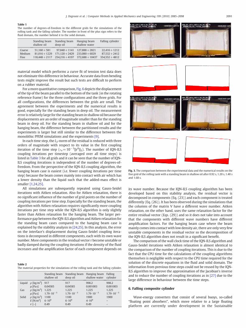
Fig. 3. The comparison between the experimental data and the numerical results on thefine grid of the rolling tank with a standing beam in shallow oil after 0.92 s, 1.20 s, 1.40 sand 1.68 s.

Table 1The number of degrees-of-freedom in the different grids for the simulations of therolling tank and the falling cylinder. The number in front of the plus sign refers to thefluid domain, the number behind it to the solid domain.

Standing beamshallow oil

Standing beamdeep oil

Hanging beamshallow water

Falling cylinder

Coarse 51,160+581 97,840+1141 127,888+2821 22,416+1212Medium 81,016+1229 171,120+2429 233,080+6029 87,532+2412Fine 118,448+2117 254,216+4197 372,688+10437 354,552+4812


material model which performs a curve fit of tension test data doesnot eliminate this difference in behaviour. Accurate data from bendingtests might improve the result but such tests are difficult to performon a rubber material.

For amore quantitative comparison, Fig. 6 depicts the displacementof the tip of the beamparallel to the bottom of the tank (in the rotatingreference frame) for the three configurations and the three grids. Forall configurations, the differences between the grids are small. Theagreement between the experiments and the numerical results isgood, especially for the standing beam in deep oil. The measurementerror is relatively large for the standingbeam in shallowoil because thedisplacements are an order ofmagnitude smaller than for the standingbeam in deep oil. For the standing beam in shallow oil and for thehanging beam, the difference between the partitioned results and theexperiments is larger but still similar to the difference between themonolithic PFEM simulations and the experiments [9].

In each time step, the L2-norm of the residual is reducedwith threeorders of magnitude with respect to its value in the first couplingiteration of the time step (�o=10−3||r0||2). The number of IQN-ILScoupling iterations per timestep (averaged over all time steps) islisted in Table 3 for all grids and it can be seen that the number of IQN-ILS coupling iterations is independent of the number of degrees-of-freedom. From the perspective of the IQN-ILS coupling algorithm, thehanging beam case is easiest (i.e. fewer coupling iterations per timestep) because the beam comes mainly into contact with air which hasa lower density than the liquid such that the added-mass effect issmaller [1,24,25].

All simulations are subsequently repeated using Gauss-Seideliterations with Aitken relaxation. Also for Aitken relaxation, there isno significant influence of the number of grid points on the number ofcoupling iterations per time step. Especially for the standing beam, thealgorithmwith Aitken relaxation requires significantly more couplingiterations per time step while the IQN-ILS algorithm is only slightlyfaster than Aitken relaxation for the hanging beam. The larger per-formance gap between the IQN-ILS algorithmandAitken relaxation forthe standing beam cases compared to the hanging beam case isexplained by the stability analysis in [24,25]. In this analysis, the erroron the interface's displacement during Gauss-Seidel coupling itera-tions is decomposed in different components, each with its own wavenumber.More components in the residual vector r become unstable orbadly damped during the coupling iterations if the density of the fluidincreases and the amplification factor of each component depends on

Table 2The material properties for the simulations of the rolling tank and the falling cylinder.




Fallingcylinder

Liquid ρ [kg/m3] 917 917 998.2 998.2μ [Pas] 0.04585 0.04585 0.001003 0.001003

Gas ρ [kg/m3] 1.225 1.225 1.225 1.225μ [Pas] 1.79·10−5 1.79·10−5 1.79·10−5 1.79·10−5

Solid ρ [kg/m3] 1100 1100 1900 1900E [N/m2] 6·106 6·106 4·106 –

ν [–] 0.49 0.49 0.49 –

its wave number. Because the IQN-ILS coupling algorithm has beendeveloped based on this stability analysis, the residual vector isdecomposed in components (Eq. (23)) and each component is treateddifferently (Eq. (26)). It has been observed during the simulations thatthe columns of the matrix V have a different wave number. Aitkenrelaxation, on the other hand, uses the same relaxation factor for theentire residual vector (Eqs. (29)) and so it does not take into accountthat the components with different wave numbers have differentamplification factors. For the hanging beam case where the beammainly comes into contactwith lowdensity air, there are only very fewunstable components in the residual vector so the decomposition ofthe IQN-ILS algorithm does not result in a significant benefit.

The comparison of the wall clock time of the IQN-ILS algorithm andGauss-Seidel iterations with Aitken relaxation is almost identical tothe comparison of the number of coupling iterations. This is due to thefact that the CPU time for the calculations of the coupling algorithmsthemselves is negligible with respect to the CPU time required for thesolution of the discrete equations in the fluid and solid domain. Theinformation from previous time steps could not be reused by the IQN-ILS algorithm to improve the approximation of the Jacobian's inverseand to reduce the number of coupling iterations as in [27] due to thelarge difference in behaviour between the time steps.

6. Falling composite cylinder

Wave-energy converters that consist of several buoys, so-called“floating point absorbers”, which move relative to a large floatingplatform are currently under development in the Sustainable

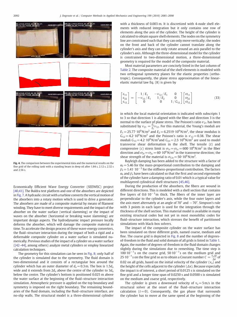
Fig. 4. The comparison between the experimental data and the numerical results on thefine grid of the rolling tank with a standing beam in deep oil after 1.84 s, 2.12 s, 2.32 sand 2.56 s.


Economically Efficient Wave Energy Converter (SEEWEC) project[40,41]. The Buldra test platform and one of the absorbers are depictedin Fig. 7. Ahydraulic circuitwitha turbine converts the verticalmotionofthe absorbers into a rotary motion which is used to drive a generator.The absorbers are made of a composite material by means of filamentwinding. They have tomeet diverse requirements and the impact of theabsorber on the water surface (vertical slamming) or the impact ofwaves on the absorber (horizontal or breaking wave slamming) areimportant design aspects. The hydrodynamic impact pressure locallydeforms the absorber, which will damage the composite material intime. To accelerate the design process of thesewave-energy converters,the fluid–structure interaction during the impact of both a rigid and adeformable composite cylinder on a water surface is simulated nu-merically. Previous studies of the impact of a cylinder on awater surface([42–44], among others) analyze metal cylinders or employ linearizedcalculation techniques.

The geometry for this simulation can be seen in Fig. 8; only half ofthe cylinder is simulated due to the symmetry. The fluid domain istwo-dimensional and it consists of a rectangular box around thecylinder which has an outer diameter of do=0.3m. The box is 1.5dowide and it extends from 2do above the centre of the cylinder to 3dobelow the centre. The cylinder's bottom is positioned 0.025 m abovethe water surface at the beginning of the fluid–structure interactionsimulation. Atmospheric pressure is applied on the top boundary andsymmetry is imposed on the right boundary. The remaining bound-aries of the fluid domain, including the fluid–structure interface, areno-slip walls. The structural model is a three-dimensional cylinder

with a thickness of 0.003 m. It is discretized with 4-node shell ele-ments with reduced integration but it only contains one row ofelements along the axis of the cylinder. The height of the cylinder iscalculated to obtain square shell elements. The nodes on the symmetryline are constrained such that they can onlymove vertically; the nodeson the front and back of the cylinder cannot translate along thecylinder's axis and they can only rotate around an axis parallel to thecylinder's axis. Although the three-dimensional model for the cylinderis constrained to two-dimensional motion, a three-dimensionalgeometry is required for the model of the composite material.

Most material parameters are concisely listed in the last column ofTable 2. The composite material of the shell elements is modeled withtwo orthogonal symmetry planes for the elastic properties (ortho-tropic). Consequently, the plane stress approximation of the linear-elastic material law Eq. (8) is given by

ε11ε22ε12

24

35 =

1 = E1 −ν12 = E1 0−ν12 = E1 1 = E2 0

0 0 1 = G12

24

35 σ11

σ22σ12

24

35 ð33Þ

in which the local material orientation is indicated with subscripts 1to 3 so that direction 1 is aligned with the fiber and direction 3 is thenormal to the surface of plane stress. The Poisson's ratio ν21 has beensubstituted by ν21 = E2

E1ν12. For this material, the Young's moduli are

E1=25.77⋅109N/m2 and E2=6.2519⋅109N/m2, the shear modulus isG12=4.2⋅109N/m2 and the Poisson's ratio is ν12=0.38. The shearmoduli G13=4.2⋅109N/m2and G23=2.5⋅109N/m2 are used to modeltransverse shear deformation in the shell. The tensile (t) andcompressive (c) stress limit is σ1t=σ1c=600⋅106N/m2 in the fiberdirection and σ2t=σ2c=60⋅106N/m2 in the transverse direction; theshear strength of the material is σ12s=50⋅106N/m2.

Rayleigh damping has been added to the structure with a factor ofαr=5.46 for the mass-proportional contribution to the damping andβr=1.41⋅10−5 for the stiffness-proportional contribution. The factorsαr and βr have been calculated so that the first and second eigenmodeof the cylinder have a damping ratio of 0.01which is a typical value formultilayered cylindrical shell structures [45,46].

During the production of the absorbers, the fibers are wound indifferent directions. This is modeled with a shell section that containsfive layers of 0.6⋅10−3m thick. The fibers of the inner layer areperpendicular to the cylinder's axis, while the four outer layers andthe axis meet alternately at an angle of 70° and −70°. Simpson's rulewith 3 points in each layer is used for the integration through thethickness of the shell section. This material model is available in manyexisting structural codes but not yet in most monolithic codes forfluid–structure interaction, which stresses the benefit of partitionedsimulations with black-box solvers.

The impact of the composite cylinder on the water surface hasbeen simulated on three different grids, named coarse, medium andfine. The coarse grid is depicted in Fig. 8 and the number of degrees-of-freedom in the fluid and solid domain of all grids is listed in Table 1.Again, the number of degrees-of-freedom in the fluid domain changesslightly during the simulations due to remeshing. The time step is100∙10−7s on the coarse grid, 50∙10−7s on the medium grid and25∙10−7s on the fine grid so as to obtain a Courant number C = voΔt

Δxof

0.02 on all grids, based on the initial velocity of the cylinder (vo) andthe height of the cells adjacent to the cylinder (Δx). Because especiallythe impact is of interest, a short period of 0.0125 s is simulated on thefine grid and a longer time span of 0.0250 s and 0.0500 s is simulatedon the medium and coarse grid, respectively.

The cylinder is given a downward velocity of vo=5m/s in thestructural solver at the onset of the fluid–structure interactioncalculation (t=0). Consequently, the gas phase that surroundsthe cylinder has to move at the same speed at the beginning of the

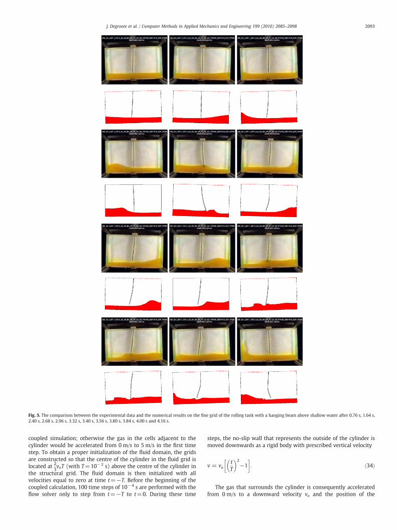
Fig. 5. The comparison between the experimental data and the numerical results on the fine grid of the rolling tank with a hanging beam above shallow water after 0.76 s, 1.64 s,2.40 s, 2.68 s, 2.96 s, 3.32 s, 3.40 s, 3.56 s, 3.80 s, 3.84 s, 4.00 s and 4.16 s.


coupled simulation; otherwise the gas in the cells adjacent to thecylinder would be accelerated from 0 m/s to 5 m/s in the first timestep. To obtain a proper initialization of the fluid domain, the gridsare constructed so that the centre of the cylinder in the fluid grid islocated at 2

3voT (with T=10−2 s) above the centre of the cylinder in

the structural grid. The fluid domain is then initialized with allvelocities equal to zero at time t=−T. Before the beginning of thecoupled calculation, 100 time steps of 10−4 s are performed with theflow solver only to step from t=−T to t=0. During these time

steps, the no-slip wall that represents the outside of the cylinder ismoved downwards as a rigid body with prescribed vertical velocity

v = votT

� �2−1

: ð34Þ

The gas that surrounds the cylinder is consequently acceleratedfrom 0 m/s to a downward velocity vo and the position of the

Table 3The number of coupling iterations per time step (averaged over all time steps andbetween brackets averaged over all time steps between t=0 and t=0.0125 s) for thesimulations of the rolling tank and the falling cylinder.




Falling cylinder

IQN-ILS Aitken IQN-ILS Aitken IQN-ILS Aitken IQN-ILS Aitken

Coarse 7.16 11.93 8.90 15.16 4.54 5.34 10.4 (7.6) 17.9 (12.6)Medium 7.32 12.11 8.95 15.40 4.53 5.14 9.5 (7.6)Fine 7.62 12.53 8.96 15.30 4.53 4.92 8.1

Fig. 6. The displacement of the tip of the beam parallel to the bottom of the tank (in therotating reference frame) for the simulation of the rolling tankwith (a) a standing beamin shallow oil, (b) a standing beam in deep oil and (c) a hanging beam above shallowwater.


centre of the cylinder is identical in the fluid and solid domain att=0.

During the fluid–structure interaction calculation, the cylinder firstfalls through the air region and then it impacts on the water surfacearound t=5∙10−3 s. There is no exact time of impact because there is

no exact position of the liquid–gas interface as this interface is nottracked with grid points but reconstructed from the volume fraction.The shape of the free-surface during the impact is displayed inFig. 9. These plots show that the cylinder is first compressed vertically(Fig. 9(c)) and then stretched vertically (Fig. 9(e)). This can also beobserved in Fig. 10(a) which depicts the deformation of the cylinder,defined as the difference between the initial and current value ofthe distance between the top and the bottom of the cylinder. Thedeformation is small while the cylinder is traversing the air regionbut it increases rapidly during the impact on the water surface. Afterthe initial contact, the deformation oscillates with decreasingamplitude. The maximal deformation amounts to approximately 6%of the cylinder's diameter.

Fig. 10(b) displays the vertical velocity at the bottom of thecylinder as a function of time. The simulation on the coarse grid hasbeen performed with the flexible cylinder as described above but alsowith a “rigid” cylinder which has thousand times larger stiffnessmoduli than the flexible cylinder. At impact, the velocity at the bottomof the cylinder jumps from−5 m/s to−2 m/s for the flexible cylinder,followed by oscillations due to the interaction between the inertia inthe flexible structure and in the fluid. The velocity decreases moregradually for the rigid cylinder as it barely deforms. The vertical forceon the entire cylinder is shown in Fig. 10(c) and the peak at impact ismuch higher for the rigid cylinder, as expected. As the force isproportional to the acceleration and thus to the second timederivative of the displacement, it is much more difficult to have asmooth evolution of the force than a smooth evolution of thedisplacement. Consequently, few authors show stresses or forces asa function of time.

Fig. 10 shows that the solution of the different grids is very close toeach other, especially for the medium and fine grid. The maximaldeformation is almost identical on all grids but there is a smalldifference in the time of impact between the coarse grid on one handand the medium and fine grid on the other hand, as can be seen inFig. 10(b) and (c). Because decreasing the time step with a factor twoon the coarse grid does not yield significant improvement, it can beconcluded that the difference is mainly due to the grid.

Fig. 11 depicts the pressure relative to the atmospheric pressure onthree different segments of the fluid–structure interface as a functionof time for the flexible and the rigid cylinder. The delay between thepeaks at the different locations can clearly be observed and theamplitude of the peak decreases as one moves away from the bottomof the cylinder. The peak of the pressure at the bottom of the cylinderis 182∙103N/m2 for the flexible cylinder and 279∙103N/m2 for the rigidcylinder, which proves that the fluid–structure interaction must betaken into account during the design process to avoid a too strong andtherefore a too costly product. The minimal pressure during theoscillations in t [0, 0.0125] s is 18∙103N/m2 below atmosphericpressure for the flexible cylinder and 3∙103N/m2 below atmosphericpressure for the rigid cylinder. The absolute pressure is in both caseshigher than the vapour pressure of pure water which is 2338N/m2 at293 K and thus no cavitation occurs.

Fig. 8. The coarse grid for the simulation of the falling cylinder. A constant pressure isimposed on the red boundary, yellow means a symmetry boundary, green is the fluiddomain and black represents a no-slip wall or the structural domain.

Fig. 7. (a) The Buldra test platform of the SEEWEC project and (b) a composite point absorber produced by means of filament winding.


The damage to the composite material due to the impact isassessed with the Tsai-Wu failure criterion in plane stress condi-tion [47] which requires that

IF = F1σ11 + F2σ22 + F11σ211 + F22σ

222 + F66σ

212 + 2F12σ11σ22b1

ð35aÞ

with

F1 =1σ1t

+1σ1c

ð35bÞ

F2 =1σ2t

+1σ2c

ð35cÞ

F11 =−1

σ1tσ1cð35dÞ

F22 =−1

σ2tσ2cð35eÞ

F66 =1

σ212s

ð35fÞ

F12 = fffiffiffiffiffiffiffiffiffiffiffiffiffiF11F22

p: ð25gÞ

The tensile and compressive strength in the fiber direction andin the transverse direction are given above. Often, the couplingcoefficient f is set to 0 so that F12 disappears. The value of IF is analyzedin all time steps near the impact and in all layers of the compositematerial. Its maximal value is 0.25 so well below the limit.

In each time step, the L2-norm of the residual is reduced with threeorders of magnitude with respect to its value in the first couplingiteration (�o=10−3||r0||2). The number of coupling iterations per timestep is displayed in Fig. 12 for the simulation on the coarse grid. About5 IQN-ILS iterations per time step are required during the first 500time steps while the cylinder is falling through air. However,approximately 11 IQN-ILS iterations per time step are necessary toreach convergence in the time steps in which there is contact betweenthe cylinder and the water. This difference illustrates the effect of thefluid density on the stability of the coupling iterations [1,24,25]. Thenumber of coupling iterations per time step (averaged over all timesteps and over all time steps between t=0 and t=0.0125s) is similar

Fig. 10. (a) The deformation of the flexible cylinder as a function of time for the fallingcylinder. The deformation is defined as the initial distance between the top and bottomof the cylinder (do) minus the current distance between the top and bottom (d). (b) Thevertical velocity at the bottom of the rigid and flexible cylinder as a function of time.(c) The vertical force on the entire rigid and flexible cylinder as a function of time.

Fig. 9. The shape of the water surface on the coarse grid of the falling flexible cylinderafter (a) 0.005 s, (b) 0.010 s, (c) 0.015 s, (d) 0.020 s, (e) 0.025 s, (f) 0.030 s, (g) 0.035 s,(h) 0.040 s and (i) 0.045 s.


for all grids as can be seen in Table 3. This proves that the performanceof the IQN-ILS coupling algorithm is independent of the number ofdegrees-of-freedom. For comparison, the simulation on the coarsegrid are also performed using Gauss-Seidel iterations with Aitkenrelaxation which requires almost twice as many coupling iterationsto reach the same convergence tolerance. The number of couplingiterations per time step is limited to 20. As in the previous section,reuse of information from previous time steps to improve theapproximation of the Jacobian's inverse and consequently reducethe number of coupling iterations as used in [27] does not functionwell in this particular case due to the large difference in behaviourbetween the time steps during the impact.

7. Conclusion

The numerical results demonstrate that the interaction betweenfree surface flow and an elastic structure can be simulated in a

partitioned way using the IQN-ILS coupling algorithm, even for caseswith strong interaction due to the incompressibility of the fluid.Gauss-Seidel iterations with Aitken relaxation can also be used butthis requires more coupling iterations. Both coupling algorithms treatthe flow solver and the structural solver as a black box, meaning

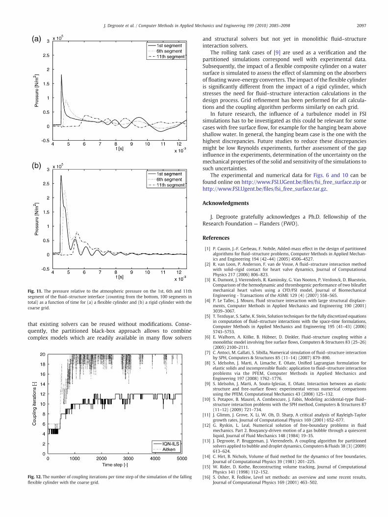
Fig. 11. The pressure relative to the atmospheric pressure on the 1st, 6th and 11thsegment of the fluid–structure interface (counting from the bottom, 100 segments intotal) as a function of time for (a) a flexible cylinder and (b) a rigid cylinder with thecoarse grid.


that existing solvers can be reused without modifications. Conse-quently, the partitioned black-box approach allows to combinecomplex models which are readily available in many flow solvers

Fig. 12. The number of coupling iterations per time step of the simulation of the fallingflexible cylinder with the coarse grid.

and structural solvers but not yet in monolithic fluid–structureinteraction solvers.

The rolling tank cases of [9] are used as a verification and thepartitioned simulations correspond well with experimental data.Subsequently, the impact of a flexible composite cylinder on a watersurface is simulated to assess the effect of slamming on the absorbersof floatingwave-energy converters. The impact of the flexible cylinderis significantly different from the impact of a rigid cylinder, whichstresses the need for fluid–structure interaction calculations in thedesign process. Grid refinement has been performed for all calcula-tions and the coupling algorithm performs similarly on each grid.

In future research, the influence of a turbulence model in FSIsimulations has to be investigated as this could be relevant for somecases with free surface flow, for example for the hanging beam aboveshallow water. In general, the hanging beam case is the one with thehighest discrepancies. Future studies to reduce these discrepanciesmight be low Reynolds experiments, further assessment of the gapinfluence in the experiments, determination of the uncertainty on themechanical properties of the solid and sensitivity of the simulations tosuch uncertainties.

The experimental and numerical data for Figs. 6 and 10 can befound online on http://www.FSI.UGent.be/files/fsi_free_surface.zip orhttp://www.FSI.Ugent.be/files/fsi_free_surface.tar.gz.

Acknowledgments

J. Degroote gratefully acknowledges a Ph.D. fellowship of theResearch Foundation — Flanders (FWO).

References

[1] P. Causin, J.-F. Gerbeau, F. Nobile, Added-mass effect in the design of partitionedalgorithms for fluid–structure problems, Computer Methods in Applied Mechan-ics and Engineering 194 (42–44) (2005) 4506–4527.

[2] R. van Loon, P. Anderson, F. van de Vosse, A fluid–structure interaction methodwith solid–rigid contact for heart valve dynamics, Journal of ComputationalPhysics 217 (2006) 806–823.

[3] K. Dumont, J. Vierendeels, R. Kaminsky, G. Van Nooten, P. Verdonck, D. Bluestein,Comparison of the hemodynamic and thrombogenic performance of two bileafletmechanical heart valves using a CFD/FSI model, Journal of BiomechanicalEngineering - Transactions of the ASME 129 (4) (2007) 558–565.

[4] P. Le Tallec, J. Mouro, Fluid structure interaction with large structural displace-ments, Computer Methods in Applied Mechanics and Engineering 190 (2001)3039–3067.

[5] T. Tezduyar, S. Sathe, K. Stein, Solution techniques for the fully discretized equationsin computation of fluid–structure interactions with the space-time formulations,Computer Methods in Applied Mechanics and Engineering 195 (41–43) (2006)5743–5753.

[6] E. Walhorn, A. Kölke, B. Hübner, D. Dinkler, Fluid–structure coupling within amonolithic model involving free surface flows, Computers & Structures 83 (25–26)(2005) 2100–2111.

[7] C. Antoci, M. Gallati, S. Sibilla, Numerical simulation of fluid–structure interactionby SPH, Computers & Structures 85 (11–14) (2007) 879–890.

[8] S. Idelsohn, J. Marti, A. Limache, E. Oñate, Unified Lagrangian formulation forelastic solids and incompressible fluids: application to fluid–structure interactionproblems via the PFEM, Computer Methods in Applied Mechanics andEngineering 197 (2008) 1762–1776.

[9] S. Idelsohn, J. Marti, A. Souto-Iglesias, E. Oñate, Interaction between an elasticstructure and free-surface flows: experimental versus numerical comparisonsusing the PFEM, Computational Mechanics 43 (2008) 125–132.

[10] S. Potapov, B. Maurel, A. Combescure, J. Fabis, Modeling accidental-type fluid–structure interaction problems with the SPH method, Computers & Structures 87(11–12) (2009) 721–734.

[11] J. Glimm, J. Grove, X. Li, W. Oh, D. Sharp, A critical analysis of Rayleigh-Taylorgrowth rates, Journal of Computational Physics 169 (2001) 652–677.

[12] G. Ryskin, L. Leal, Numerical solution of free-boundary problems in fluidmechanics. Part 2. Bouyancy-driven motion of a gas bubble through a quiescentliquid, Journal of Fluid Mechanics 148 (1984) 19–35.

[13] J. Degroote, P. Bruggeman, J. Vierendeels, A coupling algorithm for partitionedsolvers applied to bubble and droplet dynamics, Computers & Fluids 38 (3) (2009)613–624.

[14] C. Hirt, B. Nichols, Volume of fluid method for the dynamics of free boundaries,Journal of Computational Physics 39 (1981) 201–225.

[15] W. Rider, D. Kothe, Reconstructing volume tracking, Journal of ComputationalPhysics 141 (1998) 112–152.

[16] S. Osher, R. Fedkiw, Level set methods: an overview and some recent results,Journal of Computational Physics 169 (2001) 463–502.

http://www.FSI.UGent.be/files/fsi_free_surface.zip

http://www.FSI.Ugent.be/files/fsi_free_surface.tar.gz


[17] E. Oñate, S. Idelsohn, F. Del Pin, R. Aubry, The particle finite element method. Anoverview, International Journal of Computational Methods 1 (2004) 267–307.

[18] J. Monaghan, Simulating free surface flows with SPH, Journal of ComputationalPhysics 110 (2) (1994) 399–406.

[19] D. Rothman, S. Zaleski, Lattice-gas models of phase separation: interfaces, phasetransitions and multiphase flow, Reviews of Modern Physics 66 (1994)1417–1479.

[20] A. Colagrossi, M. Landrini, Numerical simulation of interfacial flows by smoothedparticle hydrodynamics, Journal of Computational Physics 191 (2) (2003)448–475.

[21] M. Heil, An efficient solver for the fully coupled solution of large-displacementfluid–structure interaction problems, Computer Methods in Applied Mechanicsand Engineering 193 (2004) 1–23.

[22] C. Felippa, K. Park, C. Farhat, Partitioned analysis of coupled mechanical systems,Computer Methods in Applied Mechanics and Engineering 190 (2001)3247–3270.

[23] C. Förster, W. Wall, E. Ramm, Artificial added mass instabilities in sequentialstaggered coupling of nonlinear structures and incompressible viscous flows,Computer Methods in Applied Mechanics and Engineering 196 (7) (2007)1278–1293.

[24] J. Degroote, P. Bruggeman, R. Haelterman, J. Vierendeels, Stability of a couplingtechnique for partitioned solvers in FSI applications, Computers & Structures 86(23–24) (2008) 2224–2234.

[25] J. Degroote, S. Annerel, J. Vierendeels, Stability analysis of Gauss-Seidel iterationsin a partitioned simulation of fluid–structure interaction, Computers & StructuresIn press.

[26] J. Vierendeels, L. Lanoye, J. Degroote, P. Verdonck, Implicit coupling of partitionedfluid–structure interaction problems with reduced order models, Computers &Structures 85 (11–14) (2007) 970–976.

[27] J. Degroote, K.-J. Bathe, J. Vierendeels, Performance of a new partitioned procedureversus a monolithic procedure in fluid–structure interaction, Computers &Structures 87 (11–12) (2009) 793–801.

[28] C. Michler, E. van Brummelen, R. de Borst, An interface Newton-Krylov solver forfluid–structure interaction, International Journal for Numerical Methods in Fluids47 (10–11) (2005) 1189–1195.

[29] H. Matthies, R. Niekamp, J. Steindorf, Algorithms for strong coupling procedures,Computer Methods in Applied Mechanics and Engineering 195 (2006)2028–2049.

[30] D. Mok, W. Wall, Partitioned analysis schemes for the transient interaction ofincompressible flows and nonlinear flexible structures, in: K. Schweizerhof, K.Wall, W.A. Bletzinger (Eds.), Trends in computational structural mechanics,CIMNE, Barcelona, 2001.

[31] U. Küttler, W. Wall, Fixed-point fluid–structure interaction solvers with dynamicrelaxation, Computational Mechanics 43 (2008) 61–72.

[32] S. Patankar, Numerical Heat Transfer and Fluid Flow, Hemisphere, Washington,DC, USA, 1980.

[33] D. Youngs, Numerical Methods for Fluid Dynamics, chap. Time-Dependent Multi-Material Flow with Large Fluid Distortion, in: K.W. Morton, M.J. Baines (Eds.),Academic Press, New York, NY, USA, 1982, pp. 273–285.

[34] H. Hilber, T. Hughes, R. Taylor, Improved numerical dissipation for timeintegration algorithms in structural dynamics, Earthquake Engineering &Structural Dynamics 5 (3) (1977) 283–292.

[35] C. Farhat, M. Lesoinne, P. Le Tallec, Load and motion transfer algorithms for fluid/structure interaction problems with non-matching discrete interfaces: momen-tum and energy conservation, optimal discretization and application toaeroelasticity, Computer Methods in Applied Mechanics and Engineering 157(1998) 95–114.

[36] A. de Boer, A. van Zuijlen, H. Bijl, Review of coupling methods for non-matchingmeshes, Computer Methods in Applied Mechanics and Engineering 196 (2007)1515–1525.

[37] R. Haelterman, J. Degroote, D. Van Heule, J. Vierendeels, The quasi-Newton leastsquares method: a new and fast secant method analyzed for linear systems, SIAMJournal on numerical analysis 47 (3) (2009) 2347–2368.

[38] G.H. Golub, C.F.V. Loan, Matrix computations, 3 rd edn.Johns Hopkins UniversityPress, Baltimore, MD, USA, 1996.

[39] H. Lamb, Hydrodynamics, Surface Waves, 6 edn, Cambridge University Press,1932, pp. 365–369, chap. 9.

[40] G. De Backer, M. Vantorre, R. Banasiak, J. De Rouck, C. Beels, H. Verhaeghe,Performance of a point absorber heaving with respect to a floating platform, 7thEuropean Wave and Tidal Energy Conference, Porto, Portugal, 1, 2007.

[41] C. Blommaert, W. Van Paepegem, J. Degrieck, Design of composite material forcost effective large scale production of components for floating offshorestructures, Plastics rubber and composites 38 (2) (2009) 146–152.

[42] M.-C. Lin, L.-D. Shieh, Flow visualization and pressure characteristics of a cylinderfor water impact, Applied Ocean Research 19 (1997) 101–112.

[43] M. Ionina, A. Korobkin, Water impact on cylindrical shells, in: R. Beck, W. Schultz(Eds.), International Workshop on Water Waves and Floating Bodies, Port Huron,MI, USA, 1999, pp. 44–47.

[44] H. Sun, O. Faltinsen, Water impact of horizontal circular cylinders and cylindricalshells, Applied Ocean Research 28 (2006) 299–311.

[45] N. Alam, N. Asnani, Vibration and damping analysis of a multilayered cylindricalshell, Part I: Theoretical analysis, AIAA Journal 22 (6) (1984) 803–810.

[46] N. Alam, N. Asnani, Vibration and damping analysis of a multilayered cylindricalshell, Part II: Numerical results, AIAA Journal 22 (7) (1984) 975–981.

[47] S. Tsai, E. Wu, General theory of strength for anisotropic materials, Journal ofComposite Materials 5 (1971) 58–80.

Documents

Computer Methods in Applied Mechanics and Engineering€¦ · the components of certain wave-energy converters. ... Computer Methods in Applied Mechanics and Engineering 199 ... Computer