Embed Size (px)
Citation preview

COMPUTER METHODS IN APPLIED MECHANICS AND ENGINEERING 82 (1990) 27-57 NORTH-HOLLAND
A DISCOURSE ON THE STABILITY CONDITIONS FOR MIXED FINITE ELEMENT FORMULATIONS
Franco B R E Z Z I Dipartimento di Meccanica Strutturale and Istituto di Analisi, Numerica del C. N.R., 27100 Pavia, Italy
Klaus-Jiirgen B A T H E Department of Mechanical Engineering, Massachusetts Institute of Technology, Cambridge, MA 02139,
U.S.A.
Received 13 February 1990
We discuss the general mathematical conditions for solvability, stability and optimal error bounds of mixed finite element discretizations. Our objective is to present these conditions with relatively simple arguments. We present the conditions for solvability and stability by considering the general coefficient matrix of mixed finite element discretizations, and then deduce the conditions for optimal error bounds for the distance between the finite element solutions and the exact solution of the mathematical problem. To exemplify our presentation we consider the solutions of various example problems. Finally, we also present a numerical test that is useful to identify numerically whether, for the solution of the general Stokes flow problem, a given finite element discretization satisfies the stability and optimal error bound conditions.
I. Introduction
During the recent years it has been recognized to an increasing extent that the use of mixed finite elements can be of great benefit and may even be necessary to obtain reliable and accurate solutions in certain fields of engineering analysis. Mixed finite elements are currently used with much success in the solution of incompressible fluid flows, and continue to provide great promise for the analysis of solids and structures [1, 2].
Of course, the largest area of finite e lement applications is still structural analysis and mixed finite elements are, in principle, much suited for use in the analysis of almost incompressible media (for example, for the analysis of rubber-like materials, elasto-plasticity and creep) and the analysis of plates and shells. However, although many mixed finite elements have been proposed over the last two decades in the research literature, it is apparent that mixed finite elements are hardly used in practical structural analysis.
The reason why mixed finite elements are not used abundantly in engineering practice is that their predictive behavior is much more difficult to assess than for the conventional and commonly used displacement-based elements. Whereas displacement-based elements, once formulated and shown to work well on certain sets of examples (including the patch tests), can be generally employed, mixed finite elements cannot be recommended for general use unless a deeper analysis and understanding is available. Namely, considering a certain category of
0045-7825/90/$03.50 © 1990 - Elsevier Science Publishers B.V. (North-Holland)

28 F. Brezzi, K.J. Bathe, A discourse on the stability conditions for FE formulations
problems, a mixed finite element may work well in the solution of certain problems but perform very poorly on other problems. Therefore, a mathematical analysis (even a limited one) for the stability and convergence of a proposed formulation is an important requirement. Such mathematical analysis should give sufficient insight as to the general applicability of the finite element under consideration, and is in general no easy task.
Some researchers have proposed some easily applied 'counting rules' to assess whether a mixed finite element can be recommended [3, 4]. However, such rules can at best give some guide-lines and do not give the necessary information to assess whether an element is stable and accurate.
Considering mixed finite element discretizations, we recognize that they are governed by a system of equations with a coefficient matrix C, that we may write as
0 ]" (1.1)
We quote as a main example the analysis of incompressible fluid flow, the Stokes problem, when using the velocity-pressure formulation. Other important examples of interest are the analysis of incompressible solids and the analysis of plates and shells. In principle, many solutions can be formulated using a mixed or hybrid method that results into the coefficient matrix (1.1), because this matrix is reached by minimizing a functional under linear con- straints [1].
The general mathematical theory for the solution of problems that are governed by the coefficient matrix in (1.1) is now quite well established and the detailed applications of this theory to a number of important problem categories is available. We know necessary and sufficient conditions for the existence and uniqueness of the solution, both for the continuous and the discretized problems. We also know necessary and sufficient conditions on the choice of the discretizations in order to have optimal error bounds [1, 5]. This information is most valuable for the design and analysis of mixed finite elements because the basic mathematical results are quite generally applicable (while the detailed application to problem areas may of course not be straight-forward).
Our objective in this paper is two-fold. The first aim is to present the general mathematical results quoted above with relatively simple arguments. For this purpose we consider the general coefficient matrix of mixed finite element formulations and deduce the conditions of solvability and stability. In proceeding this way, we refer to the continuous problem only when necessary (since the treatment of the continuous problem requires a background in functional analysis) and we concentrate on the discretized (finite-dimensional) problem. However, we succeed in pointing out the basic mathematical conditions on the discretization and in showing that they are necessary to have stability and optimal error estimates.
Our second aim in this paper is to propose a simple numerical procedure for checking whether the above mathematical conditions are satisfied for a given mixed finite element formulation. Such a procedure is useful because it may be employed to check a formulation and its computer program implementation (much like the patch test is used for incompatible displacement-based finite element formulations). We consider in this discussion the analysis of incompressible fluid flow and our test is closely related to 'Fortin's trick' to identify whether the mathematical conditions of stability and optimal error bounds are satisfied.
F. Brezzi, K.J. Bathe, A discourse on the stability conditions for FE formulations 29
The paper is organized into the following sections. In Section 2 we recall some basic properties of square matrix systems and introduce the basic concepts of stability and optimality. In Section 3 we then deal with the special case of systems of the form (1.1); hence here we focus onto the analysis of mixed finite element formulations in detail. Finally, in Section 4 we discuss two applications and introduce our test for checking the good quality of a given discretization, using as an example the case of an incompressible fluid. We then conclude our presentation in Section 5.
2. Some preliminaries and the general problem of solvability and stability
Let us consider the general case of an N × N matrix M and the associated system
G i v e n b ~ R N f i n d x E R N such that M x = b . (2.1)
The following theorem is a well-known cornerstone in linear algebra.
T H E O R E M 2.1. Problem (2.1 ) has a unique solution for every given right-hand side b, if and only i f the associated homogeneous system Mx = 0 has only the solution x = O.
In other words, in order to have a solvable problem in (2.1) for every possible b ~ R N we need the following condition to hold:
i f M x = 0 , t h e n x = 0 . (2.2)
Condition (2.2) answers the problem of the solvability of (2.1) but not of its stability. Roughly speaking, we would like that a small change in b determines only a small change in x. However, in order to measure the magnitude of such change we have to introduce norms. Assume that we choose a norm II IlL for measuring the size of solutions and a norm II IIR for right-hand sides. In principle, we are allowed to choose the same norm for both, but we shall see that this, in general, is not the most convenient choice. We also point out explicitly that, in finite-dimensional spaces, all norms are equivalent in the sense that for any two norms 1[ IIs, and II [Is2 in R N there exist two positive constants s 1 and s z such that
II vllsl slllolls2, (2.3)
Ilvlls= s211vllsl (2.4)
for every vector v in •u. However, these constants s a and s 2 will, in general, depend on the dimension N.
E X A M P L E . This is a very simple example, only used to fix our ideas [2]. Let
Ilollsl := m a x Io, I = IIo11,, (2.5)
Ilvlls= = Io,] = 11o11,1, (2.6) i
30 F. Brezzi, K.J. Bathe, A discourse on the stability conditions for FE formulations
then it is easy to see that
so that S 1
that
max Iv, I ~ E Iv,I, (2.7) i i
E IOil ~ N max Ili[, (2.8) i i
= 1 and s z = N. Similarly we have for the Euclidean norm,
IlvllE:= Iv, I 2 =lloll/2, (2.9)
lie I1,1~< x/-~llv 11,2, Ilvll,<.V-~llvlllo. (2.10)
We have seen that the choice of one norm or another can change, asymptotically, the dependence on N of the various constants. We shall come back to this point with useful guidelines for the most convenient choices. For the moment, we assume that the choice of II IlL and II I1~ has been performed and define stability in terms of these norms.
D E F I N I T I O N . Let M be a non-singular N × N matrix. We define the stability constant of M with respect to the norms II IlL and II IIR as the smallest possible constant SLR such that
II~bll~ II~xllL ~< sL~ (2.11) IlxllL Ilbll.
for all vectors x and 8x in R u with M x =: b and M 8x =: 8b. []
In other words, (2.11) bounds the relative change in x (in the norm L) by means of the relative change in the right-hand side b (in the norm R). We point out that such a constant SLR always exists. However, if we consider a sequence of problems of type (2.1) with increasing dimension N (corresponding, in general, to a finer and finer finite element mesh) we might find that the corresponding constants SLR depend on N and become infinitely large when N----> +o0. Thus we might say that a sequence of problems of the type (2.1) is stable with respect to the norms II I1~ and II I1~ if the stability constant SLR is uniformly bounded.
We would like now to present stability from a slightly different point of view. For this, let us introduce the matrix norms
and
IIMYlIR IIMII~. = sup - - (2.12) Y I l Y l I '
IIM-1IIRL = sup I l M - l z l l ' (2.13) z Ilzll~
From (2.13) for z = 8b (so that M - l z = ~X) we easily obtain
II~xllL (2.14) IIM-~IIRL ~ II~bll------~ '
F. Brezzi, K.J. Bathe, A discourse on the stability conditions for FE formulations 31
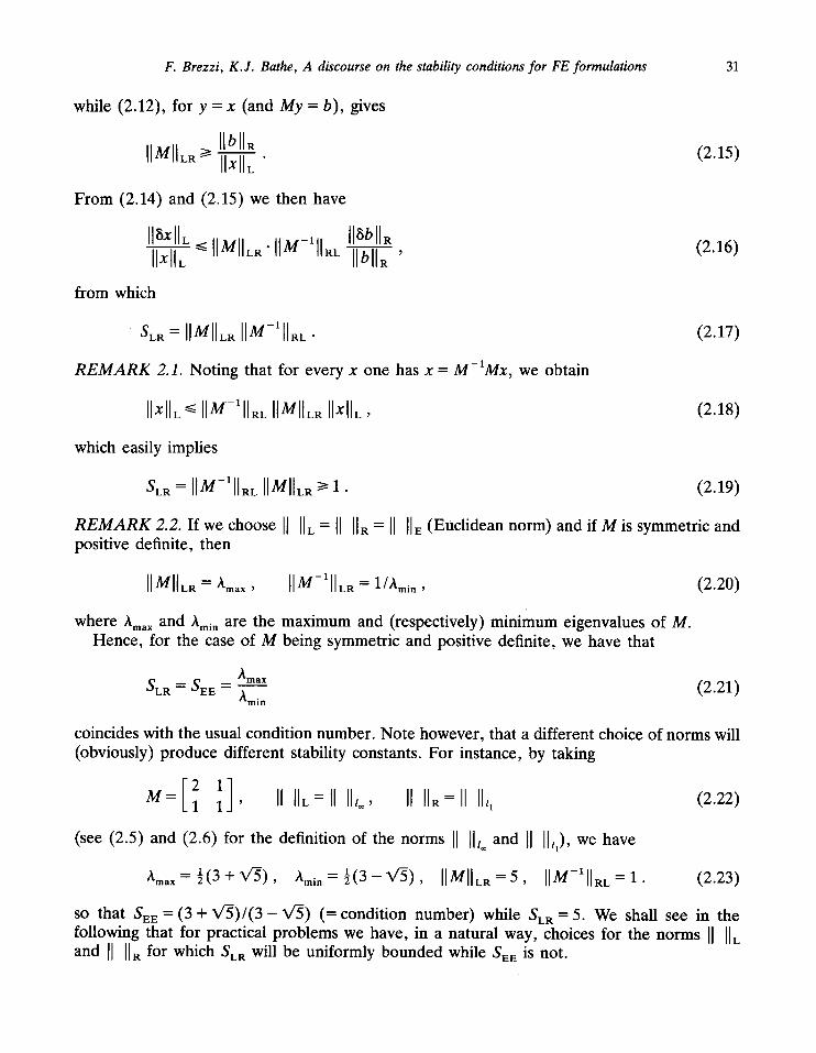
while (2.12), for y = x (and My = b), gives
IlbllR IIMIILR >I Ilxl-----~ (2.15)
From (2.14) and (2.15) we then have
II~xll, (2.16) Ilxll---7 -< IIMII,~" IIM-111~L II~bll_____~ Ilbll~ '
from which
SL~ = IIMIILR IIM-XII~L • (2.17)
REMARK 2.1. Noting that for every x one has x = M-IMx, we obtain
IIxlIL ~ IIM-'II~L IIMIIL~ IIXIIL, (2.18)
which easily implies
SL~ = IIM-1IIRL IIMIILR I> 1. (2.19)
R E M A R K 2.2. If we choose II IlL = II I1~ ----II lie (Euclidean norm) and if M is symmetric and positive definite, then
IIMIIL~ = A m a x , IIM-1IIL~ ~- a/~.rnin , (2.20)
where hma x and Ami . are the maximum and (respectively) minimum eigenvalues of M. Hence, for the case of M being symmetric and positive definite, we have that
/~max (2.21) SLR = SEE -- '~min
coincides with the usual condition number. Note however, that a different choice of norms will (obviously) produce different stability constants. For instance, by taking
1 1 ' II ILL--II I1,o, II I1~ = II I1,, (2.22)
(see (2.5) and (2.6) for the definition of the norms II I1,~ and II II,), we have
'~rnax = ½(3 + X/5), '~rnin = ½(3- V ~ ) , IIMIILR -- 5, IIM-XII~L = 1. (2.23)
so that SEE = (3 + V ~ ) / ( 3 - V~) (= condition number) while SLR = 5. We shall see in the following that for practical problems we have, in a natural way, choices for the norms II IlL and II I1~ for which SLR will be uniformly bounded while SEE is not.

32 F. Brezzi, K.J. Bathe, A discourse on the stability conditions for FE formulations
From (2.17) we see that a sequence of problems will be stable with respect to the norms II IlL and II 114 if both IIMIIL~ and IIM-XII~ are uniformly bounded. In the applications it is very easy to find norms II I1~ such that
y'Mx~kMllYllL Ilxll, Vx, y , (2.24)
with k M uniformly bounded from above and from below. From (2.24) we have a natural choice for II IIR that produces a uniform bound for IIMIIL~. Indeed, if we define the dual norm of II IlL by
IIzlIDL := sup ytz (2.25) y IlylIL '
we have the following proposition.
PROPOSITION 2.1. Let M be an N x N matrix, let II IlL be a norm in R iv and let k M be the smallest possible constant for which (2.24) holds true, that is,
ytMx k M = sup . (2.26)
x , y IlylIL Ilxll,
I f we choose II I1~ = II I1~ (dual norm o f II IlL as defined in (2.25)), then
IIMII~ = k ~ . (2.27)
PROOF. We have
IIMxlIR IIMIILR = sup IIxlI------T (use (2.12))
IIMxlIoL = s u p
x IIxlIL (use II IIR = II IIDL)
{ ll~[~ L y 'Mx ~ = sup sup (use (2.25)) x y II--~L J
ytMx = sup - k M (use (2.26)).
x,y Ilxll~ IlylIL [] (2.28)
If we assume now that we are given a sequence of problems such that
ytMx<~kMllYllLllXHL Vx, y ,
with k M uniformly bounded from above and from below, and if we choose l[ 114 = II IIDL, then the sequence of problems will be stable with respect to the norms I[ IlL and i] ]]R if and only if IIM-Xll~L is uniformly bounded. In the following proposition we express IIM-111~L in terms of the norm II IlL alone.
F. Brezzi, K.J. Bathe, A discourse on the stability conditions for FE formulations 33
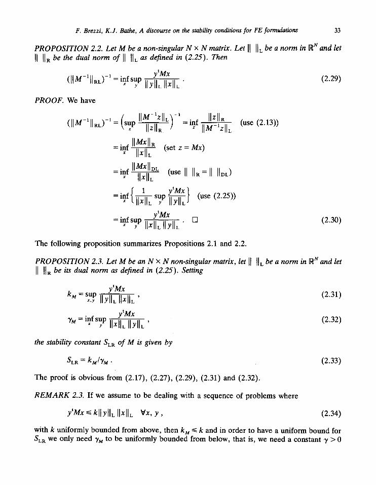
P R O P O S I T I O N 2.2. Let M be a non-singular N x N matrix. Let II II, be a norm in R N and let II I1~ be the dual norm of II II, as defined in (2.25). Then
(IIM-~II~0 -~ = inf sup ytMx (2.29) Y IlylIL Ilxll~"
PROOF. We have
([IM-1IIRL) -1= (sup Z
)-1 IlzllR IIM-lzll~ =in f (use (2.13)) IlzllR ~ IIM-lzll~
IIMxll~ =in f Ilxll~ (set z Mx)
=inf IIMxlIDL (use II I1~= II IIoL) Ilxll,
1 ytMx =in f [-~LSUPI[--~L J (use (2.25))
ytMx [] (2.30) = inf sup
The following proposition summarizes Propositions 2.1 and 2.2.
P R O P O S I T I O N 2.3. Let M be an N × N non-singular matrix, let II IlL be a norm in R N and let II IIR be its dual norm as defined in (2.25). Setting
ytMx k M = sup , (2.31)
x,r Ilyll~ IIxlIL ytMx
YM = inf sup , (2.32) x ~ IIxlILIlylI~
the stability constant SLR of M is given by
SLR = kM/YM. (2.33)
The proof is obvious from (2.17), (2.27), (2.29), (2.31) and (2.32).
R E M A R K 2.3. If we assume to be dealing with a sequence of problems where
Y tMX ~ kllYlIL IlxllL Vx, y , (2.34)
with k uniformly bounded from above, then k M <<. k and in order to have a uniform bound for SLR we only need YM to be uniformly bounded from below, that is, we need a constant y > 0
34 F. Brezz~, K.J. Bathe, A discourse on the stability conditions for FE formulations
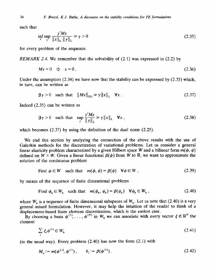
such that y t M x
infsup t> > 0 (2.35) x y IIXlILIlYlIL '/
for every problem of the sequence.
R E M A R K 2.4. We remember that the solvability of (2.1) was expressed in (2.2) by
M x = O ~ x = 0 . (2.36)
Under the assumption (2.34) we have now that the stability can be expressed by (2.35) which, in turn, can be written as
3 , / > 0 such that IIMXlIDLI>'/IIxlI Wx. (2.37)
Indeed (2.35) can be written as
3y >0 such that sup y t M x Y ~ ~ ' / I I x l I L Vx, (2.38)
which becomes (2.37) by using the definition of the dual norm (2.25).
We end this section by analyzing the connection of the above results with the use of Galerkin methods for the discretization of variational problems. Let us consider a general linear elasticity problem characterized by a given Hilbert space W and a bilinear form m(~b, qJ) defined on W × W. Given a linear functional/3(th) from W to R, we want to approximate the solution of the continuous problem
Find ~b ~ W such that m(th, ~b) =/3(qJ) VqJ ~ W , (2.39)
by means of the sequence of finite dimensional problems
Find qb h E W h such that m(dPh, ~Oh) = fl(~Oh) VqJ h ~ W h , (2.40)
where W h is a sequence of finite dimensional subspaces of W h. Let us note that (2.40) is a very general mixed formulation. However, it may help the intuition of the reader to think of a displacement-based finite element discretization, which is the easiest case.
By choosing a basis ~b (1), . . , ~b (N) in W h we can associate with every vector ~ E R N the element
wh i
(in the usual way). Every problem (2.40) has now the form (2.1) with
(2.41)
Mi j := rn(~b (j), ~b(i)), b i := fl(~b(i)). (2.42)

F. Brezzi, K.J. Bathe, A discourse on the stability conditions for FE formulations 35
If the bilinear form m(4,, q,) satisfies
m(4,, ~0)~k~l14 ,11~ IIq'll~ V4,, q ~ W , (2 .43)
then (2.34) will easily hold with k = k m (with k m independent of h) if we choose
i4, w (i) (2.44)
as a norm in R N. The stability condition (2.35) can now be written in terms of the bilinear form m(4,, ~b) and of the space W h as
m( 4,h , ~bh ) inf sup
¢~hEWh *h~'Wh 114,hllw II~IIw t>3 ,>0 (2.45)
with 3' independent of h. We point out that (2.45) on one hand implies (as we have seen) the solvability of every
discrete problem (2.40). On the other hand, if (2.45) holds with 3, independent of h, then one can deduce optimal error bounds for the distance between the solution 4' of (2.39) and the solution 4,h of (2.40). Incidentally, we point out that (2.45), together with
l im{ inf ile-e~llw)=o v ~ e w (2.49) h-.O ~,hew h
implies that (2.39) has a unique solution. We shall not report here the proof of this fact (which has basically little bearing upon our discussion), and shall instead report the proof of the optimal error bounds.
T H E O R E M 2.2 [6]. Assume that the bilinear form m(4,, ~k) and the sequence o f subspaces W h C W satisfy (2.43), (2.45) and (2.49). Let 4> be the solution o f (2.39) and 4,h the solution o f (2.40). Then
114, - 4,~llw ~<(1 + kin~3, ) inf 114,- q'~llw • ~th e W h
(2 .50)
PROOF. For every ~kh E W h we have
3, II q,h - 4,~11 ~ ~ sup Xh E W h
m(~bh -- 4,h, Xh) IIx~ll~
(use (2.45))
= sup )(h E Wh
{m(O/h -- 4,, Xh) -- m(4, -- 4,h, Xh)}
m( q'h -- 4,, Xh ) ---- s u p
(add and subtract 4,)
(use (2.39) and (2.40)
~< sup (use (2.43)) Xh~h IIxhll~
= kmll~0h - 4,11w • (2 .51)
36 F. Brezz~, K.J. Bathe, A discourse on the stability conditions for FE formulations
From (2.51) we have, using the triangle inequality,
II ch - ¢ II w ~< II ch - ~h II w + II ~,~ - 6 II w
<~ ( k m / Y ) l l o h - 611w + I1~,~ - ¢llw
= (1 + km/Y)llg'h - ¢ l l w
and (2.50) follows since (2.52) holds for every ¢'h E W h. []
(2.52)
3. Solvability and stability of mixed finite element formulations
We consider now a special case of (2.1). Namely we assume that the matrix M has the typical form arrived at when using a mixed finite element formulation,
[A ° M = B ' (3.1)
where A is a square N A × N A matrix and B a rectangular N B × N A matrix with (obviously) N A + N B = N . Accordingly we split the unknown x = (u, p) with u ~ R NA and p C R NB and the right-hand side b = (f , g) with f ~ W vA, g E R NB. With this notation, the linear system under examination can be written as
A u + B t p = f , B u = g . (3.2)
The analysis of the solvability, stability and optimality of mixed formulations has been performed in [5]. However, we shall follow here the more elegant presentation of Arnold [7]. In any case, the following space is of crucial importance. We set
K = {v E f f ~ N A I B v =0}
(in other words K = Ker(B)). Let N K be the dimension of K; we can split R/vA as
(3.3)
If N T is the dimension of T, we will obviously have N T + N K = N A .
Let us now assume that the system of equations with the matrix M has been established in a suitable basis so that we can write the matrix A as
A rr ] (3.6) A T K o
A = A K r AKK
~ N A = T ~ K , (3.4)
where T is the orthogonal of K in R NA. As a consequence of (3.4) every v ~ R NA can be split, in a unique way, as a sum
v v r + o K with o r E T, v K ~ K and t = v r v K = O. (3.5)
F. Brezzi, K.J. Bathe, A discourse on the stability conditions for FE formulations 37
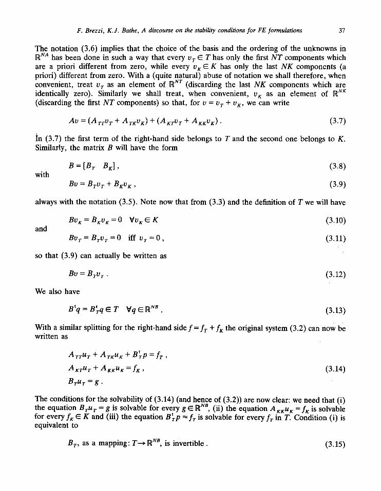
The notation (3.6) implies that the choice of the basis and the ordering of the unknowns in R NA has been done in such a way that every v r E T has only the first N T components which are a priori different from zero, while every v r ~ K has only the last N K components (a priori) different from zero. With a (quite natural) abuse of notation we shall therefore, when convenient, treat o r as an element of R Nr (discarding the last N K components which are identically zero). Similarly we shall treat, when convenient, v K as an element of R NK
(discarding the first N T components) so that, for v = o r + v r , we can write
A v = ( A f r o r + A r r V K ) + ( A f r o r + AKKVK) . (3.7)
in (3.7) the first term of the right-hand side belongs to T and the second one belongs to K. Similarly, the matrix B will have the form
with B = [ B v BKI, (3.8)
Bo = Bro r + B r o r , (3.9)
always with the notation (3.5). Note now that from (3.3) and the definition of T we will have
and Bv r = B r v r = O Vv r E K (3.10)
By r = B r v T = O iff v r = 0 , (3.11)
so that (3.9) can actually be written as
Bv = B r v r . (3.12)
We also have
Btq = Btrq ~ T Vq E R N8 . (3.13)
With a similar splitting for the right-hand side f = f r + fK the original system (3.2) can now be written as
t A r r u r + A r r u r + B r P = f r ,
A r r u r + A r r u r = f r ,
B r u r = g •
(3.14)
The conditions for the solvability of (3.14) (and hence of (3.2)) are now clear: we need that (i) the equation B r u r = g is solvable for every g E R NB, (ii) the equation A r r u r = f x is solvable for every f r E K and (iii) the equation Btrp = fT is solvable for every fT in T. Condition (i) is equivalent to
BT, a s a mapping: T---> R NB, is invertible. (3.15)
38 F. Brezzi, K.J. Bathe, A discourse on the stability conditions for FE formulations
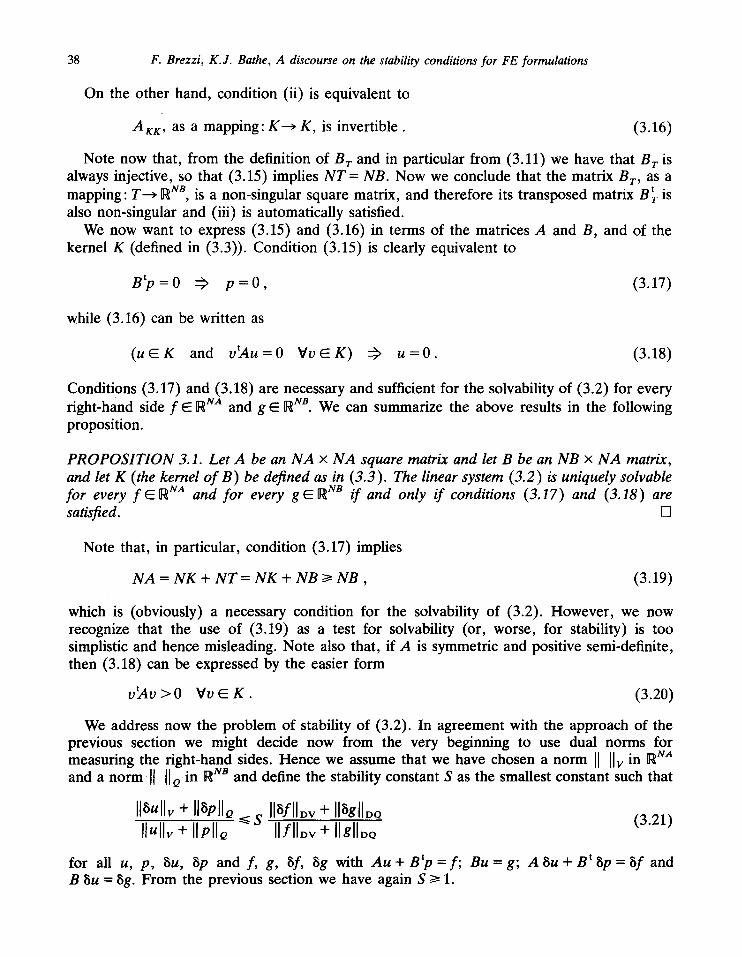
On the other hand, condition (ii) is equivalent to
AKK, as a mapping: K---> K, is invertible. (3.16)
Note now that, from the definition of B r and in particular from (3.11) we have that B r is always injective, so that (3.15) implies N T = NB. Now we conclude that the matrix Br, as a mapping: T---> R NB, is a non-singular square matrix, and therefore its transposed matrix B~- is also non-singular and (iii) is automatically satisfied.
We now want to express (3.15) and (3.16) in terms of the matrices A and B, and of the kernel K (defined in (3.3)). Condition (3.15) is clearly equivalent to
B t p = 0 z:) p = 0 , (3.17)
while (3.16) can be written as
( u C K and v tAu=O V v ~ K ) :ff u = 0 . (3.18)
Conditions (3.17) and (3.18) are necessary and sufficient for the solvability of (3.2) for every right-hand side f ~ •NA and g E R NB. We can summarize the above results in the following proposition.
P R O P O S I T I O N 3.1. Let A be an N A x N A square matrix and let B be an N B x N A matrix, and let K (the kernel o r B ) be defined as in (3.3). The linear system (3.2) is uniquely solvable for every f ~ N A and for every g E R NB i f and only i f conditions (3.17) and (3.18) are satisfied. []
Note that, in particular, condition (3.17) implies
N A = N K + N T = N K + N B >>- N B , (3.19)
which is (obviously) a necessary condition for the solvability of (3.2). However, we now recognize that the use of (3.19) as a test for solvability (or, worse, for stability) is too simplistic and hence misleading. Note also that, if A is symmetric and positive semi-definite, then (3.18) can be expressed by the easier form
vtAv > 0 Vv E K . (3.20)
We address now the problem of stability of (3.2). In agreement with the approach of the previous section we might decide now from the very beginning to use dual norms for measuring the right-hand sides. Hence we assume that we have chosen a norm II IIv in R Na
N B and a no rm I I Iio in R and define the stability constant S as the smallest constant such that
IlSullv + IlSpllo Ilullv+llpllo
IlafllDv + IlagllDo (3.21) IlfllDv + IlgllDo
for all u, p, 8u, 8p and f, g, 8f, 8g with A u + Btp = f; Bu = g; A 8u + B t 8p = 8 f and B 8u = 8g. From the previous section we have again S I> 1.
F. Brezzi, K.J. Bathe, A discourse on the stability conditions for FE formulations 39
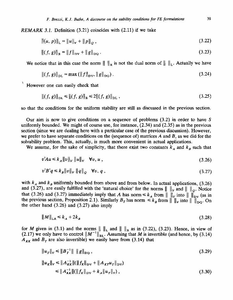
R E M A R K 3.1. Definition (3.21) coincides with (2.11) if we take
II(u, P)II~ = Ilull~ + IIPlIo, (3.22)
II(f, g)llR = I[fllDv + IlgllD~ • (3.23)
We notice that in this case the norm II IIR is not the dual norm of II I1,. Actually we have
II(L g)llD~ = max (llfl lov, Ilgll~Q) •
However one can easily check that
(3.24)
II(f, g)IIDL ~ II(f' g)llR ~ 211(f, g)IIDL, (3.25)
so that the conditions for the uniform stability are still as discussed in the previous section.
Our aim is now to give conditions on a sequence of problems (3.2) in order to have S uniformly bounded. We might of course use, for instance, (2.34) and (2.35) as in the previous section (since we are dealing here with a particular case of the previous discussion). However, we prefer to have separate conditions on the (sequence of) matrices A and B, as we did for the solvability problem. This, actually, is much more convenient in actual applications.
We assume, for the sake of simplicity, that there exist two constants k a and k B such that
o~u<~kal lo l l~ Ilull¢ Vv, u, (3.26)
v'n'q~llvll~ IlqllQ Vu, q , (3.27)
with k a and k B uniformly bounded from above and from below. In actual applications, (3.26) and (3.27), are easily fulfilled with the 'natural choice' for the norms II IIv and II IIQ. Notice that (3.26) and (3.27) immediately imply that A has norm ~< k a from II IIv into II II~v (as in the previous section, Proposition 2.1). Similarly B r has norm ~< k B from II I1~ into II IIDo. On the other hand (3.26) and (3.27) also imply
IIMII~R ~ ka + 2kB (3.28)
for M given in (3.1) and the norms II IlL and II ItR as in (3.22), (3.23). Hence, in view of (2.17) we only have to control IIM -111RL Assuming that M is invertible (and hence, by (3.14) A r K and B r are also invertible) we easily have from (3.14) that
IluTIl~ ~ l ln~ l l l Ilgll~Q, (3.29)
IlUKIIv ~ IIA~LII(II fKIIDv ÷ IIAKTU~IIDv)
IIAT~II(II fKII~v + kAIlu~llv), (3.3o)
40 F. Brezzi, K.J. Bathe, A discourse on the stability conditions for FE formulations
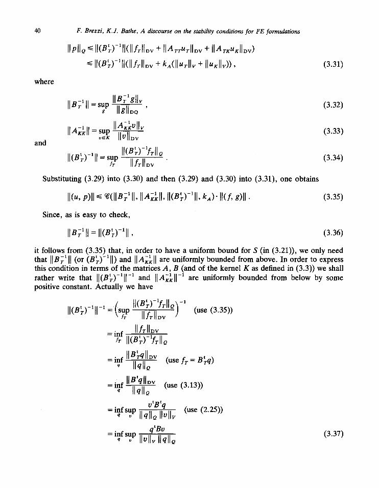
[IpIIQ ~ II(B~)-lll(llfrll~v ÷ [IA~u~llov ÷ IIA~,~uKllov) II(B~)-lll(llfrllDv ÷ ka(llu~ll~ ÷ Ilu,~ll~)), (3.31)
where
and
IIB;II[ = sup IlB~lgllv (3.32) g Ilgll.o '
IIA;~II = sup IlA;~vllv (3.33) o ~ IlollDv
II(B~)-Iw~IIQ II(n~)-lll = sup (3.34)
:T [I/~l[Dv
Substituting (3.29) into (3.30) and then (3.29) and (3.30) into (3.31), one obtains
II(u, p)ll ~ ~(IIB;~ II, IIA~II, I[(n~)-lll , kA)" II(f, g)ll . (3.35)
Since, as is easy to check,
IIB;~[[ : II(B~)-~II, (3.36)
it follows from (3.35) that, in order to have a uniform bound for S (in (3.21)), we only need that [[Br I [[ (or (Br)-~[[) and [[A~[[ are uniformly bounded from above. In order to express this condition in terms of the matrices A, B (and of the kernel K as defined in (3.3)) we shall rather write that [[(B~)-~[[ -1 and [[Arl[[ -~ are uniformly bounded from below by some positive constant. Actually we have
II(B~)-lll -I = (sup [l(B~)-lfrllQ~-I " ¢r [[-'~r[[~v ] (use (3.35))
= in f IIA-II.v fT II(B~.)-I/~.lIQ
=inf II~-qlIDv (use f~.= Bh,) IIqlIQ
=inf IIB'qllDv (use (3.13)) q IIqlIQ
°tBtq (use (2.25)) = inf sup q o [[q[[QllolIv
q tBo = inf sup
q o IIollv IlqlIQ (3.37)
F. Brezzi, K.J. Bathe, A discourse on the stability conditions for FE formulations 41
and
IIA7,~11-1= (sup IIA~:~'vllv~-I (use (3.33)) "veX" ~ ]
= inf Ilvllov Axxvll~
= i n f Ilmxxullov (use v = axxu) u~X Ilull~
z t A KK u = inf sup (use (2.25))
ztAu = inf sup (use (3.7)). (3.38)
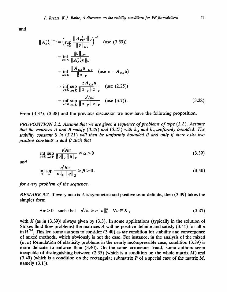
From (3.37), (3.38) and the previous discussion we now have the following proposition.
PROPOSITION 3.2. Assume that we are given a sequence of problems of type (3.2). Assume that the matrices A and B satisfy (3.26) and (3.27) with kA and k B uniformly bounded. The stability constant S in (3.21) will then be uniformly bounded if and only if there exist two positive constants ot and [3 such that
v~Au inf sup >I a > 0 (3.39) u~xo~x Ilvllv Ilullv
and
inf sup q tBO q o Ilvl lvIIqllo ~ > 8 > ° " (3.40)
for every problem of the sequence.
R E M A R K 3.2. If every matrix A is symmetric and positive semi-definite, then (3.39) takes the simpler form
3 a > 0 such that o~Ao~l lv l l L VoEK, (3.41)
with K (as in (3.39)) always given by (3.3). In some applications (typically in the solution of Stokes fluid flow problems) the matrices A will be positive definite and satisfy (3.41) for all v in R NA. This led some authors to consider (3.40) as the condition for stability and convergence of mixed methods, which obviously is not the case. For instance, in the analysis of the mixed (o-, u) formulation of elasticity problems in the nearly incompressible case, condition (3.39) is more delicate to enforce than (3.40). On the same erroneous trend, some authors seem incapable of distinguishing between (2.35) (which is a condition on the whole matrix M) and (3.40) (which is a condition on the rectangular submatrix B of a special case of the matrix M, namely (3.1)).
42 F. Brezzi, K.J. Bathe, A discourse on the stability conditions for FE formulations
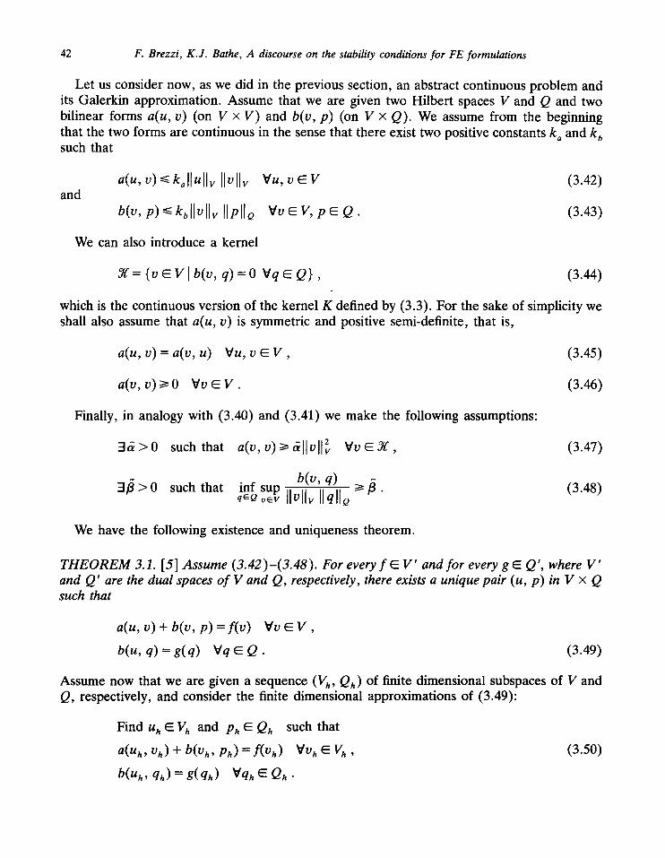
Let us consider now, as we did in the previous section, an abstract continuous problem and its Galerkin approximation. Assume that we are given two Hilbert spaces V and Q and two bilinear forms a(u, v) (on V x V) and b(v, p) (on V × Q). We assume from the beginning that the two forms are continuous in the sense that there exist two positive constants k s and k b such that
and a(u, v) <~ k~llullv Ilvllv
b(v, p) ~ kollvllv Ilpllo
Vu, v E V (3.42)
Vv ~ V, p ~ Q . (3.43)
We can also introduce a kernel
Y ( = { v E V I b ( v , q ) = O V q E Q } , (3.44)
which is the continuous version of the kernel K defined by (3.3). For the sake of simplicity we shall also assume that a(u, v) is symmetric and positive semi-definite, that is,
a(u, v) = a(v, u) Vu, v E V , (3.45)
a(v, v) >>- 0 Vv ~ V . (3.46)
Finally, in analogy with (3.40) and (3.41) we make the following assumptions:
2 V v E ~ (3.47) 3 & > 0 such that a(v,v)>>-&llvllv
b(v, q) 3/3 > 0 such that inf sup t>/3. (3.48)
q~Q oEV IIvlIv Ilqllo
We have the following existence and uniqueness theorem.
THEOREM 3.1. [5] Assume (3.42)-(3.48). For every f E V ' and for every g E Q', where V ' and Q' are the dual spaces of V and Q, respectively, there exists a unique pair (u, p) in V x Q such that
a(u, v) + b(v , p ) = f ( v ) Vv E V ,
b(u, q) = g(q) Vq E Q . (3.49)
Assume now that we are given a sequence (V h, Qh) of finite dimensional subspaces of V and Q, respectively, and consider the finite dimensional approximations of (3.49):
Find u h E Vh and Ph E Qh such that
a(Uh, Oh) + b(Vh, Ph) =]:(Oh) VVhEVh, (3.50) b(Uh, qh) = g( qh) Vqh E Qh "

F. Brezzi, K.J. Bathe, A discourse on the stability conditions for FE formulations 43
It will also be convenient to introduce the finite dimensional kernels
~g h = {o h E V h I b(Vh, qh) = 0 Vqh E Qh} " (3.51)
It is clear that, by choosing bases in V h and Oh, (3.50) can be written in the form (3.2). As a consequence, the solvability conditions for (3.50) will be
a(Vh, V h) > 0 VV h ~ ~ h , (3.52)
{b(Vh'qh)=O Vv hEVh} ~ qh=O, (3.53)
as it can easily be deduced from (3.20) and (3.17). The uniform stability conditions now become
3 4 * > 0 such that a(vh, Vh)~*llvhll~ V V h ~ C h , (3.54)
3/3* > 0 such that inf sup b(vh, qh) /3, (3.55) qhEQh VhEV h Ilvhll~ IlqhllQ ~> '
with or* and/3* independent of h. It is clear that (3.54) and (3.55) are just a different way of writing (3.41) and (3.40). It is also clear that (3.54) implies (3.52), and (3.55) implies (3.53), so that stability implies solvability.
As far as error estimates are concerned we have the following theorem.
T H E O R E M 3.2. [5] Assume that the sequence o f subspaces (Vh, Qh) satisfies (3.54) and (3.55). Then problem (3.50) has a unique solution (Uh, Ph) for every h > O. Moreover there exists a constant c > O, depending only on k a (3.42), k b (3.43), a* (3.54) and/3* (3.55) such that
Ilu- uhll~ + lip -PhlIQ ~ C{ inf Ilu- ohllv + inf l ip - qhllQ} (3.56) Oh •Vh qh ~ Qh '
where (u, p) is the solution o f (3.49).
PROOF. We shall only sketch the proof, which is based on a classical 'stability-consistency' argument. Let u~, and p~, be the best approximation one can have for u and p, respectively, in the subspaces, that is,
Ilu- u~lIv = inf Ilu- ohllv, Vh ~ V h
(3.57)
I l p - p ~ l I Q = inf I I P - q h l I Q . qh ff-Qh
Let now
(3.58)
f(Vh) "= a(u~, Vh) "~- b(Vh, p~) , (3.59)
g( qh) := b(u~, qh) , (3.60)
44 F. Brezzi, K.J. Bathe, A discourse on the stability conditions for FE formulations
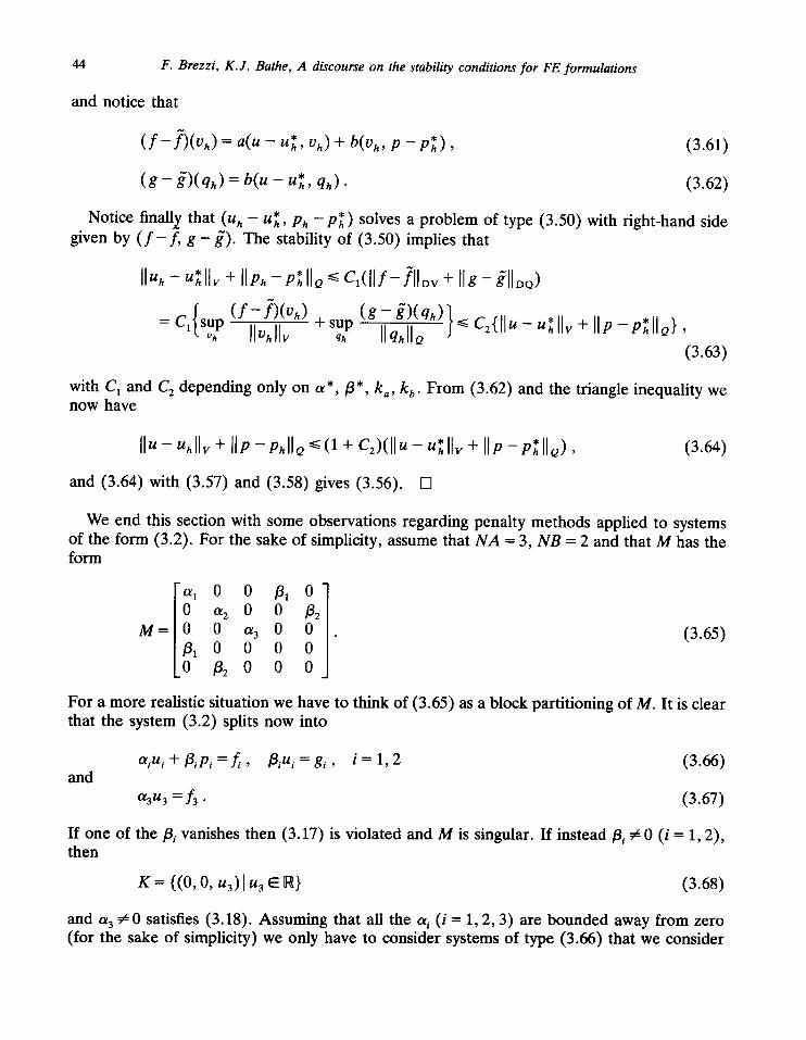
and notice that
( f -- f ) (vh) = a ( u - u~,, Vh) + b(Vh, p - -p 'h) , (3.61)
( g - ff)(qh) = b ( u - u~, qh) " (3.62)
Notice finall X that (u h - u~, Ph --P*h ) solves a problem of type (3.50) with right-hand side given by ( f - f , g - ~). The stability of (3.50) implies that
Iluh - u*~llv + Ilph -p~IIQ ~ c l ( l l f - fllDv + [ I g - fflIDQ)
CI/su p ( f - f)(Vh) + sup (g -- ff)(qh) I - - oh Ilv~ll~ qh Wq-~Q " <<- C=(llu - u~ll~ ÷ lip - p ~ l l o } ,
(3.63)
with C x and C 2 depending only on Ol now have
*,/3*, k a, k b. From (3.62) and the triangle inequality we
I l u - u h l l v + l i p - PhlIQ ~<(1 + c 2 ) ( l l u - u ~ l l v + I I p - p ~ I I Q ) , (3.64)
and (3.64) with (3.57) and (3.58) gives (3.56). []
We end this section with some observations regarding penalty methods applied to systems of the form (3.2). For the sake of simplicity, assume that N A = 3, N B = 2 and that M has the form
Vii ° ° il ol2 0 2 M = 0 Ol3 0 . :10000
/32 0 0 0
(3.65)
For a more realistic situation we have to think of (3.65) as a block partitioning of M. It is clear that the system (3.2) splits now into
and olin, ÷ /3 iPi = f i , /3iUi = g i , i = 1, 2 (3 .66)
ol3u3 = L . (3.67)
If one of the/3; vanishes then (3.17) is violated and M is singular. If instead/3i # 0 (i = 1, 2), then
K = {(0 , 0, u3)lu3 ~ R) (3.68)
and a 3 # 0 satisfies (3.18). Assuming that all the a; (i = 1, 2, 3) are bounded away from zero (for the sake of simplicity) we only have to consider systems of type (3.66) that we consider

F. Brezzi, K.J. Bathe, A discourse on the stability conditions for FE formulations 45
through their typical representative:
a u + / 3 p = f , /3u = g . (3.69)
A penalty approach to (3.69) consists in finding, for e > 0 (and 'small'), the solution of
a u ~ + / 3 p ~ = f , /3u , - ep~ = g , (3.70)
which is given by
ef +/3g /3f- ~g u~ = e a + /32 , P~ = e a + /32 • ( 3 . 7 1 )
It is clear that (for a ~ 0) the solution (3.70) always exists, even for/3 = 0. However, for /3 = 0, p,---> ~ as e---> 0 when g ~ 0. On the other hand, in some applications (as, for instance, incompressibility conditions with zero Dirichlet boundary conditions), we have g = 0, and the situation improves. For g = 0 (3.71) becomes
~f /3f u~ = e a + /32 , P" = ea + /32 • (3.72)
For/3 = 0 (3.72) gives
f u~ = - , p~ = 0 , (3.73)
which is a nice result. Actually a closer look at (3.69) for /3 = g = 0 shows a singular but compatible system with solution u = f / a , p = undetermined. Clearly (3.73) gives the solution of minimum norm.
Let us now consider the case g = 0 and/3 very small. The system (3.69) will have a very large stability constant. However, if we look only at the u, component of (3.72), we have
u ~ 0 for e ~ 0 (/3 fixed) (3.74)
and u, is uniformly bounded (in e) as e goes to zero. On the other hand
u~---> f f o r / 3 - * 0 (e fixed), (3.75) ot
which shows that we have difficulties to interpret the results even if u~ is computed as a number of reasonable size. A look at the p, part of the solution shows that
p,---> f for e---->0 (/3 fixed) (3.76) /3
If/3 is very small, p~ will be very large and this indicates that a change in discretization may be required.
46 F. Brezzi, K.J. Bathe, A discourse on the stability conditions for FE formulations
In a practical analysis, there will generally be only a limited number of the /3i's that are small. Hence, only the corresponding pi components will be large, and this can explain the appearance of the so-called checker-board modes that appear, even when u, behaves nicely. Note also that, when solving with the penalty approach (for g = 0) a small/3; can be more dangerous than a/3; = 0, as shown by (3.73) compared with (3.74) and (3.76).
4. Examples of applications
In this section we present two examples that demonstrate the theory we have presented in the earlier part of the paper, and we also present a numerical procedure to test whether the inf-sup condition is satisfied for a finite element formulation to solve Stokes fluid flow problems.
4.1. Mixed methods for linear second-order elliptic problems
We start here with a very simple example to show the importance of the condition (3.54) (~h-ellipticity). Consider the mixed formulation of the model problem
4, " =1 = i n ] - l , l [ ,
The solution is clearly
~(x) = ½(x 2 - 1).
Introducing the additional variable
O" : I ] / t ,
the mixed formulation of (4.1) now reads
f ~ ~z dx + f j ~,z ' dx = O W 1
which is clearly of the form (3.49) with
v= {~-~ L2(]-1, l[) l , ' e L2(]-1, 1[),
e = e2(] -1 , 1D, II~IIQ = I1~110,
a(o',~-)=f~ o'~-dx b(z, ~b)= f2 1 ' 1
q,(-1) = ~(1) = 0.
I1~11~ = I1~11~ + I1~'110 ~ ,
~bz' dx,
(4.1)
(4.2)
(4.3)
(4.4)
(4.5)
(4.6)
(4.7)
(4.8)
F. Brezzi, K.J. Bathe, A discourse on the stability conditions for FE formulations 4 7
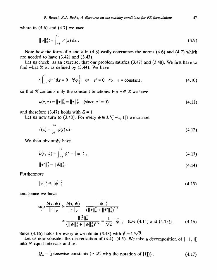
where in (4.6) and (4.7) we used
Iloll~ := f ~ o2(x) dx . (4.9)
Note how the form of a and b in (4.8) easily determines the norms (4.6) and (4.7) which are needed to have (3.42) and (3.43).
Let us check, as an exercise, that our problem satisfies (3.47) and (3.48). We first have to find what ~ is, as defined by (3.44). We have
{fJl ~bz 'dx=0 Vth} ¢:> r ' = 0 ¢:> r = c o n s t a n t , (4.10)
so that ~ contains only the constant functions. For ~- G Y( we have
a(z, z )= I1~11~ = II~IIL (since r ' =0 ) (4.11)
and therefore (3.47) holds with ~ = 1. Let us now turn to (3.48). For every q~ E L2(]-1 , 1[) we can set
~:(x) = fo q~(t) d t . (4.12)
We then obviously have
_- f~ ,~2= I1,~11,~, (4.13) b (,.?, q~)
I1÷'11o ~ = I1,~11,~ • (4.14)
Furthermore
I1÷11~ I1~11~ (4.15)
and hence we have
b(r, (~) b(~, q~) I1,~11~o - - ~ - - = 2 ~ 1 / 2 sup~ II~llv II÷llv (11~11~0+11~'110,
I1~11~ 1 (11~110 z + II~ll0Z) 1'2 - v ~ I1~110 (use (4.14) and (4.15)). (4.16)
Since (4.16) holds for every ~ we obtain (3.48) with/3 = 1/~/2. Let us now consider the discretization of (4.4), (4.5). We take a decomposition of ] - 1 , 1[
into N equal intervals and set
Qh = {piecewise constants (---Lp0 with the notation of [1])} . (4.17)

48 F. Brezzi, K.J. Bathe, A discourse on the stability conditions for FE formulations
It would now be reasonable to take
V h = (piecewise linear continuous functions (= ZP~)}. (4.18)
In this case it is easy to check that ~h is also reduced to the constant functions, and therefore (3.54) holds with a * = 1 (always by (4.11)). On the other hand the construction (4.12) still works, since q~ E ~ 0 ° implies ? E Aq11. Hence (3.55) also holds, with/3* = 1/V~, and the assumptions of Theorem 3.2 are fulfilled. In our particular case ( g - 1) it is also easy to prove that, for every decomposition, we have
trh(X ) = X in ]--1, 1[, (4.19)
which is the exact solution. Assume now, for our discussion, that we take a larger Vh, namely
V h = {piecewise quadratic continuous functions (= ~ ) } . (4.20)
Setting
B E = {piecewise quadratic functions vanishing at the subdivision nodes}, (4.21)
we easily have
Vh = c~1 = ~,~11 ~) B2 " (4 .22)
We can now make an observation which is of general validity: the choice of a larger V h (with the same Qh) makes the inf-sup condition (3.55) easier to satisfy and the ~h-ellipticity condition (3.54) more difficult to satisfy (unless, obviously, the bilinear form a is V-elliptic: in such a case (3.54) is always satisfied for all choices of V h and Qh). In our case
/ =o (4.23)
where ~ is the space of global constants as in (4.10). Let now, for every subinterval Ik(k = 1 , . . . , N) , b k be the second order polynomial vanishing at the endpoints of I k and normalized in such a way that
ft, b2k(X) dx = 1. (4.24)
A simple computation shows that
Ilb ll0 = lO /h , (4.25)
so that
a(bk, bk) = Ilbkll0 = 1 (4.26)
F. Brezzi, K.J. Bathe, A discourse on the stability conditions for FE formulations 49
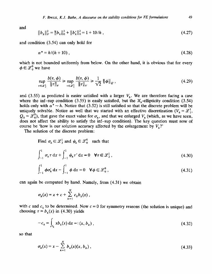
and r 2
Ilbkll = IIb ll + IIb ll0 = 1 + l O / h , (4.27)
and condition (3.54) can only hold for
a* = h / ( h + 10), (4.28)
which is not bounded uniformly from below. On the other hand, it is obvious that for every ~b E Lp0 we have
sup b(r, d~) >I sup b(r, ~b) I> 1 (4.29)
and (3.55) as predicted is easier satisfied with a larger V h. We are therefore facing a case where the inf-sup condition (3.55) is easily satisfied, but the 9~h-ellipticity condition (3.54) holds only with a* - h. Notice that (3.52) is still satisfied so that the discrete problem will be uniquely solvable. Notice as well that we started with an effective discretization ( V h = ~ , Qh = ~0) , that gave the exact value for trh, and that we enlarged V h (which, as we have seen, does not affect the ability to satisfy the inf-sup condition). The key question must now of course be 'how is our solution accuracy affected by the enlargement by Vh?'
The solution of the discrete problem:
Find o- h ~ ~12 and qJh ~ ~0 such that
f•,trh•'dx+f] ~bhT'dx=0 Vr~x2 (4.30) X
1 ~O'~ dx - - J_ (~ dx = 0 Vth E 3? 0 (4.31) r l
1
can again be computed by hand. Namely, from (4.31) we obtain
N
h(x) = x + c + c k b k ( x ) , k = l
with c and c k to be determined. Now c = 0 for symmetry reasons (the solution is unique) and choosing ~- = bk(X ) in (4.30) yields
- c k = fz k Xbk(X ) dx =: (x, bk) , (4.32)
so that
N
Oh(X ) = X -- ~ , bk(X)(X , bk) , (4.33) k = l
50 F. Brezzi; K.J. Bathe, A discourse on the stability conditions for FE formulations
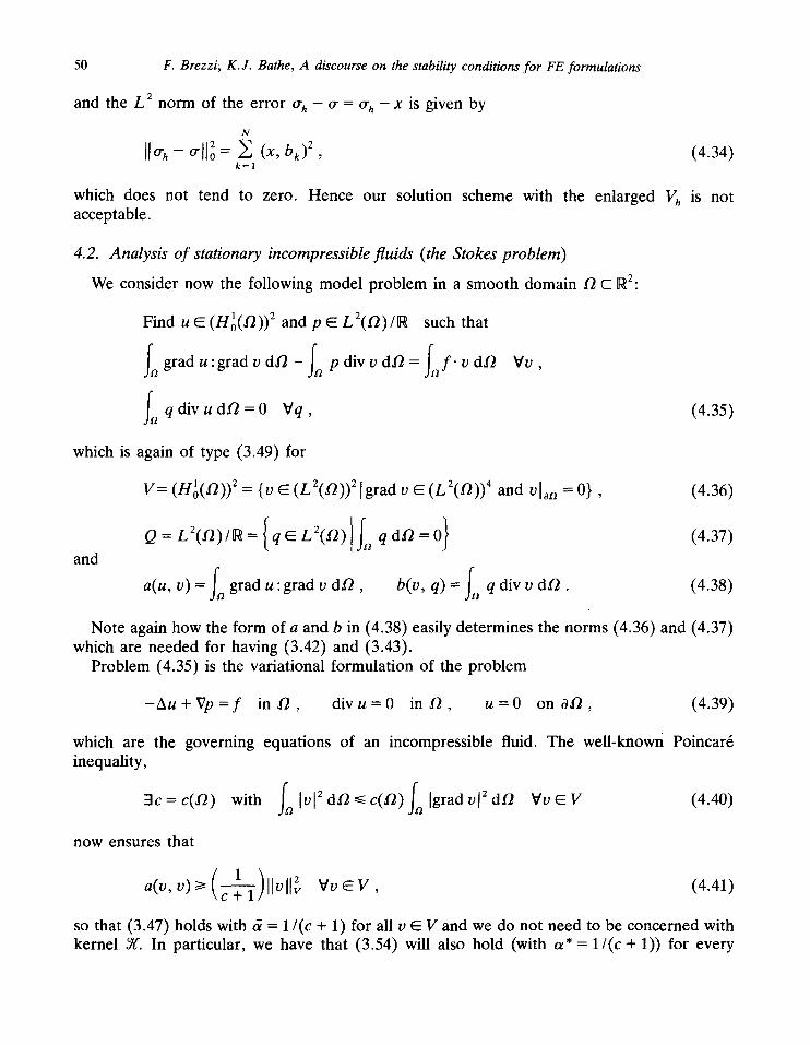
and the L 2 norm of the error er h - o" = o" h - x is given by
N
- 1120 = ( x , b k ) 2 , k = l
which does not tend to zero. Hence our solution scheme with the enlarged acceptable.
4.2. Analysis of stationary incompressible fluids (the Stokes problem) We consider now the following model problem in a smooth domain /2 C R2:
Find u E (H1(/2)) 2 and pC L2(/2)/R such that
fngradu:gradvdO-fa pdivvd12=faf , vdO Vv,
fa qdivudl2=O Vq,
which is again of type (3.49) for
V= (H~(/2)) 2 = {v ~ (L2(/2))2 [grad v E (L2(/2))4 and rio n = 0},
Q= L2(/2)/R= { q E L2(/2) l fn
a(u, v) = fa grad u :grad v d O ,
(4.34)
V h is not
and
(4.35)
f b(o, q) = Ja q div o d O . (4.38)
Note again how the form of a and b in (4.38) easily determines the norms (4.36) and (4.37) which are needed for having (3.42) and (3.43).
Problem (4.35) is the variational formulation of the problem
- A u + V p = f in /2 , d i v u = 0 i n O , u = 0 on 0/2 , (4.39)
which are the governing equations of an incompressible fluid. The well-known Poincar6 inequality,
3 c = c ( / 2 ) with f lvl2d/2<-c(O)folgradvl2d/2 Vv~V (4.40)
now ensures that
(1) a(o,v) >- ~ IIo11 , v o e v , (4.41)
so that (3.47) holds with ~ = 1/(c + 1) for all v E V and we do not need to be concerned with kernel Yg. In particular, we have that (3.54) will also hold (with a~*= 1/(c + 1)) for every
(4.36)
qd/2 =0} (4.37)
F. Brezzi, K.J. Bathe, A discourse on the stability conditions for FE formulations 51
choice of V h C V and Qh C Q. Hence we can concentrate our attention on (3.48) and (3.55), that is, on the inf-sup condition. As far as (3.48) is concerned we remark that we actually have
fn q div v dO 3/3(O) > 0 such that inf sup I>/3(O), (4.42)
IlqllQ Ilvll
which is a nontrivial result in functional analysis (see, e.g., [8, 9]). We also notice that the following result obviously holds as an immediate consequence of (4.42): for every set ~ with
(Ho~(O)) 2 c_ ~ c_ ( H i ( O ) ) 2 , (4.43)
we have
inf sup fa q div v dO qEQ vEOl: Ilqllo Ilvllv (4.44)
since the supremum over ~ is obviously larger than the supremum over V = (H0~(O)) 2. In a sense we can therefore say that the case of homogeneous Dirichlet boundary conditions is the most difficult to treat. This is the reason why we shall mainly concentrate on this case only.
Assume now that we are given a sequence of finite dimensional subspaces V h E V and Qh E Q and consider the discrete problem:
Find u h E V h and Ph E Oh
a(Uh, Vh) - b(Vh, Ph) = fa
b(Uh, qh )=O Vqh E Qh .
such that
f " Vh dO VVh ~ Vh ,
(4.45)
As we have observed above, we only have to check condition (3.55) in order to have solvability, stability and optimal error bounds. The following theorem, known as 'Fortin's trick' (see [10]) is often useful in order to prove (3.55) (see e.g. [11]).
T H E O R E M 4.1. Assume that (3.48) holds and that, for every h, we can build a linear operator II h • V---> V h with the following properties:
b(v - HhV, qh) = 0 VV E V Vqh E Qh, (4.46)
3 3 / > 0 such that I I / / hv l l~3 / l lv l l . Vv V, (4.47)
where 3/is independent o f h. Then (3.55) holds with [3* = f313/.
PROOF. We have for every qh E Qh
b(Vh, qh) b(IIhv, qh) sup I> sup
oh vh Ilohllv II//hvll
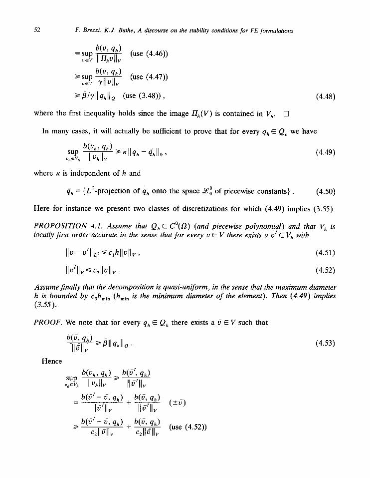
52 F. Brezzi, K.J. Bathe, A discourse on the stability conditions for FE formulations
b(v, qh) = sup (use (4.46))
o~v II//~vll~ b(v, qh)
>I sup (use (4.47))
/>/~/~llqhllQ (use (3.48)), (4.48)
where the first inequality holds since the image Hh(V ) is contained in V h. []
In many cases, it will actually be sufficient to prove that for every qh E Qh we have
b(Vh, qh) sup t> KIIq~ - 4~110 (4.49) oh~Vh IIv~IIv
where K is independent of h and
qh = {L2"pr°j ecti°n of qh onto the space ~ of piecewise constants}. (4.50)
Here for instance we present two classes of discretizations for which (4.49) implies (3.55).
PROPOSITION 4.1. Assume that Qh C C°(~-~) (and piecewise polynomial) and that V h is locally first order accurate in the sense that for every v ~ V there exists a v I E V h with
IIv-v'll,2<-Clhllvll,, (4.51)
Ildll~ ~ c~lloll~ (4.52)
Assume finally that the decomposition is quasi-uniform, in the sense that the maximum diameter h is bounded by C3hmi n (hmi n is the minimum diameter o f the element). Then (4.49) implies (3.55).
PROOF. We note that for every qh E Oh there exists a 6 E V such that
Hence
b(6, qh)
11611~ ~l lqhl lQ" (4.53)
b(Vh, qh) b( 61, qh) sup I>
b ( 5 ' - 6, qh) b(5, qh) + (+_6)
116'11~ 116'11~ b ( 6 1 - 6, qh) b(6, qh)
i> + (use (4.52)) c211611v c211611v
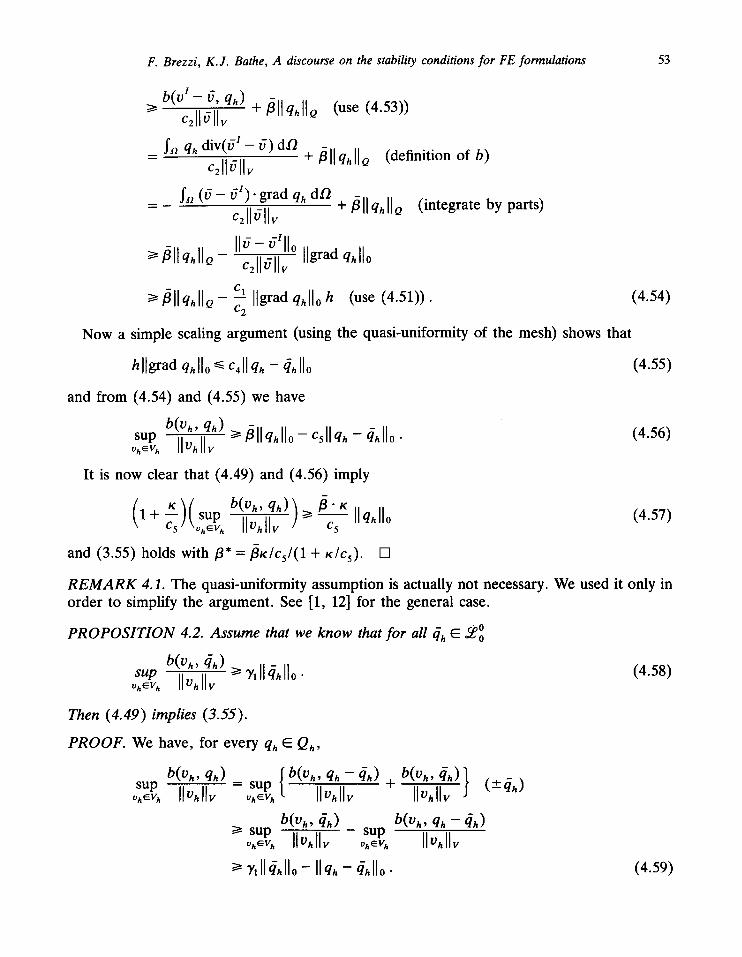
F. Brezzi, K.J. Bathe, A discourse on the stability conditions for FE formulations 53
b ( v ' - 6, qh) + ~llq~llQ (use (4.53))
fgl qh div( 61 - 6) dO
c~ll~ll. + ~llq~llQ (definition of b)
fa ( 6 - 6I).grad qh dO
c~ll~ll~ +~llq~llQ (integrate by parts)
~l lq , llQ - I1~- ~'11o ilgra d qh]lO czll~ll~
cl Ilgrad qhl loh (use (4.51)) I> t~llq~llQ - c2 (4.54)
Now a simple scaling argument (using the quasi-uniformity of the mesh) shows that
hllgrad qhllO ~ c41lqh - 4~11o (4.55)
and from (4.54) and (4.55) we have
b(Vh' qh) sup I> t~ll q, l lo - c, llq~ - 4,11o • (4.56)
It is now clear that (4.49) and (4.56) imply
(1+ f--)(sup b(Vh'qh))>~fl 'K Ilqhll0 (4.57)
and (3.55) holds with/3* = flK/cs/(1 + K/cs). []
REMARK 4.1. The quasi-uniformity assumption is actually not necessary. We used it only in order to simplify the argument. See [1, 12] for the general case.
PROPOSITION 4.2. Assume that we know that for all [lh ~ ~
b(Vh, qh) sup I> ~lll4~llo • (4.58) oh~h IIvhll~
Then (4.49) implies (3.55).
PROOF. We have, for every qh E Qh,
b(Vh, qh) ~ b(Vh, qh - - q h )
°hevhSUp IIo~llv - OhevhSUp ]. I1~11~
b(vh, qh) >I sup
b(Vh, qh) } (++-qh) + IIo~llv
b(Vh, qh -- qh) sup
• 1114,11o- Ilqh - 4,11o • (4.59)
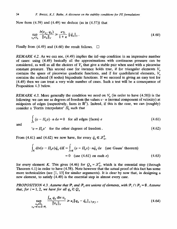
54 F. Brezzi, K.J. Bathe, A discourse on the stability conditions for FE formulations
Now from (4.59) and (4.49) we deduce (as in (4.57)) that
b(Vh, qh) KZ sup i> I1, 110 (4.60)
oh vh II Oh
Finally from (4.49) and (4.60) the result follows. []
R E M A R K 4.2. As we can see, (4.49) implies the inf-sup condition in an impressive number of cases: using (4.49) basically all the approximations with continuous pressure can be considered, as well as all the choices of V h that give a stable pair when used with a piecewise constant pressure. This second case for instance holds true, if for triangular elements V h contains the space of piecewise quadratic functions, and if for quadrilateral elements, V h contains the reduced (8 nodes) biquadratic functions. If we succeed in giving an easy test for (4.49) then we can treat a very wide number of cases. Such a test will be a consequence of Proposition 4.3 below.
R E M A R K 4.3. More generally the condition we need on V h (in order to have (4.58)) is the following: we can use as degrees of freedom the values v. n (normal component of velocity) at midpoints of edges (respectively, faces in R3). Indeed, if this is the case, we can (roughly) consider a 'Fortin interpolator' I I h such that
and f (V -- IlhV ) • n de = 0 for all edges (faces) e
'v = I lhv ' for the other degrees of f reedom.
(4.61)
(4.62)
From (4.61) and (4.62) we now have, for every qh E ~0,
fK div(v - HhV)4 h d K = Jar (v - HhV ) • nqh de (use Gauss' theorem) f
= 0 (use (4.61) on each e) (4.63)
for every element K. This gives (4.46) for Qh = *°97°, which is the essential step (through Theorem 4.1) in order to have (4.58). Note however that the actual proof of this fact has some more technicalities (see [1, 13] for similar arguments). It is clear by now that, in designing a new element, to satisfy (4.49) is the essential step in almost every case.
P R O P O S I T I O N 4.3. A s s u m e that ~1 and ~2 are unions o f elements, with ~ l fq ~2 = ~. A s s u m e that, f o r i = 1, 2, we have f o r all qh ~ Qh
f~'i qh div v h sup >t K~ll qh -- Zth I[ L2<~,) , (4.64)
Vh~V h I l o h l I v Vh=O in J'] \~i
F. Brezzi, K.J. Bathe, A discourse on the stability conditions for FE formulations 55
then
f~lU~2 qh div v h sup
Oh=O in 12 \(~1U9~2)
KIIq~ - qh II L~(~,u~) (4.65)
for all qh E Qh and with
r I> min(K~, K2). (4.66)
p R O O F . The proof is elementary. From (4.64) we have, for all qh E Qh, tWO elements O i 1 2 E ( n 0 ( ~ ) ) ~ V h (i = 1, 2), such that
and b( Oi, qh)= K,l[qh- 4~11~(~,) (4.67)
IIo'II~ ~< IIq, -- 4hll~(~,) • (4.68)
Taking v = v I J r V 2 we have
and
2
b(v, qh) ~ K~llqh - 2 >_ = -- qhllL2(,,) ~ Kllqh - qhll2z(,lu~2) i=1
Iloll~, = II0111~ + IIo211~, ~ Ilqh - qh l122<~, lu ,e )
(use (4.66)) (4.69)
(4.70)
and (4.69) with (4.70) implies (4.65). []
R E M A R K 4.4. The condition ~1 N ~2 = t~, as we can see from the proof, is not crucial. Its only purpose is to avoid a factor 2 in (4.69) and (4.70). However, we always think of using the result in the 'disjoint' case.
R E M A R K 4.5. In (4.64), (4.65) the choice of tlh as an element by element projection onto the space ~ 0 of piecewise constants is unnecessary. We might as well use a 'patch by patch' projection, that is, we might assume that t~h is constant in every patch (and equal to the mean value of qh)" On the other hand, the choice qh = 0 (which would give directly the inf-sup condition without passing through Propositions 4.1 and 4.2) is not allowed. If qh has zero mean value o n ~1 L~ ~[)2 it does not necessarily have zero mean value separately on ~1 and on ~2. But (4.64) is unrealistic if the right-hand side does not have zero mean value. Finally let us note that, if qh is the element by element projection and t~h is the patch by patch projection, then
I I q - ~hllL2 ~ IIq-- 4hilL2 •
R E M A R K 4.6. Proposition 4.3 deals with two patches. It is clear that the argument applies as well to any finite number of patches: the smallest Kg gives the global K.
R E M A R K 4.7. It is very important to point out that conditions (4.64) do not depend on the
56 F. Brezzi, K.J. Bathe, A discourse on the stability conditions for FE formulations
size of the patches. Assume that we have, for a given patch, say, of size one
f~' qh div V h sup I> Ilqh - qh 11~2~) (4.71)
for all qh E Qh(~), where Vh(~ ) is a finite element subspace of ( H I ( ~ ) ) 2 and Q h ( ~ ) is a finite element subspace of L 2 ( ~ ) and finally C~h is the mean value of qh on ~. If we shrink ~ to a small patch ~s of size h by the change of variable,
~ x = ~ / h , ~ E ~ , (4.72)
and if we change the finite element spaces accordingly, we have
J'~*' qh div v h s sup s I> KIIqh -- ~llL2~,s~ (4.73)
exactly with the same K as in (4.71). The same is true if, instead of the change of variable (4.72), we apply any other change of
variable which is 'affine', that is with constant Jacobian: actually a distortion in the shape might change r to some 8 • r , where 8 depends on the amount of distortion (essentially if J is the Jacobian matrix, 8 will depend on I1-11 • IIJII 2 and IJl" 111-1112), and for reasonable distortions r will remain greater than zero.
Proposition 4.3 and all the remarks after it suggest now a strategy for checking the inf-sup condition, if we have a continuous pressure field or if we know already that the velocity space V h under consideration can be used with piecewise constant pressures. Assume that we can find a finite number of 'representative patches', ~1, ~2, . • •, ~R, such that one can cover the decomposition with affine images of the ~i's. For each patch ~i we then check if the discrete problem is uniquely solvable on the patch (for both velocity and pressure) with homogeneous Dirichlet boundary conditions for velocities and obviously discarding the constant value of the pressure on the patch. If this is true, then a constant K i must exist; we do not need to compute it, we just want to know that it exists. Finally, the smallest Ki will give the constant K in (4.49) and the inf-sup condition will hold.
5. Concluding remarks
Our objective in this paper was to review and discuss conditions for the stability of mixed finite element formulations. We also presented a numerical test that can be employed to check whether a given mixed finite element formulation for the general Stokes problem satisfies the mathematical conditions of stability and optimal error bounds.
While the general mathematical theory for mixed formulations is quite well established, both for the continuous and discretized problems, the actual detailed use of that theory for the design and analysis of mixed finite element formulations can be a very difficult task. We note that quite effective mixed finite elements that satisfy the mathematical conditions of stability

F. Brezzi, K.J. Bathe, A discourse on the stability conditions for FE formulations 57
and optimal error bounds are available for the solution of incompressible fluid flow [1] and the analysis of incompressible or almost incompressible solid media [1, 14, 15]. Howeve r , the situation is quite different, for example, in the field of analysis of plate and shell structures [16]. He re numerous mixed finite e lements have been p roposed but mathematical analyses are hardly available. Indeed the construction of effective mixed plate and shell e lements that can be analysed and satisfy t h e mathematical condit ions of stability and optimal error bounds is very difficult, and such elements are now under active research, see for example [16-18].
References
[1] F. Brezzi and M. Fortin, Mixed and Hybrid Finite Element Methods, to appear. [2] K.J. Bathe, Finite Element Procedures in Engineering Analysis (Prentice-Hall, Englewood Cliffs, NJ, 1982). [3] O.C. Zienkiewicz, S. Qu, R.L. Taylor and S. Nakazawa, The patch test for mixed formulations, Internat. J.
Numer. Methods Engrg. 23 (1986) 1873-1883. [4] O.C. Zienkiewicz and D. Lefebvre, Three-field mixed approximation and the plate bending problem, Comm.
Appl. Numer. Methods 3 (1987) 301-309. [5] F. Brezzi, On the existence, uniqueness, and approximation of saddle-point problems arising from Lagrange
multipliers, RAIRO B-R2 (1974) 129-151. [6] I. Bahu~ka, The finite element method with Lagrangian multipliers, Numer. Math. 20 (1973) 179-192. [7] D.N. Arnold, Discretization by finite elements of a model parameter dependent problem, Numer. Math. 37
(1981) 405-421. [8] O. Ladyzhenskaya, The Mathematical Theory of Viscous Incompressible Flows (Gordon and Breach,
London, 1969). [9] R. Temam, Navier-Stokes Equations (North-Holland, Amsterdam, 1977).
[10] M. Fortin, An analysis of the convergence of mixed finite element method, RAIRO Anal. Num6r. 11 (1977) 341-354.
[11] F. Brezzi and K.J. Bathe, Studies of finite element procedures--The inf-sup condition, equivalent forms and applications, in: K.J. Bathe and D.R.J. Owen, Eds., Reliability of Methods for Engineering Analysis (Pineridge, Swansea, 1986).
[12] R. Verffirth, Error estimates for a mixed finite element approximation of the Stokes equations, RAIRO 18 (1984) 175-182.
[13] M. Fortin, Old and new finite elements for incompressible flows, Internat. J. Numer. Methods Fluids 1 (1981) 347-364.
[14] J.T. Oden and N. Kikuchi, Finite element methods for constrained problems in elasticity, Internat. J. Numer. Methods Engrg. 18 (1982) 701-725.
[15] T. Sussman and K.J. Bathe, A finite element formulation for nonlinear incompressible elastic and inelastic analysis, Comput. & Structures 26 (1/2) (1987) 357-409.
[16] A.K. Noor, T. Belytschko and J.C. Simo, eds. Analytical and Computational Models of Shells (ASME, New York, 1989).
[17] F. Brezzi, K,J. Bathe and M. Fortin, Mixed-interpolated elements for Reissner/Mindlin plates, Internat. J. Numer. Methods Engrg. 28 (1989) 1787-1801.
[18] K.J. Bathe, S.W. Cho, M.L. Bucalem and F. Brezzi, On our MITC plate bending/shell elements, in: A.K. Noor, T. Belytschko and J.C. Simo, eds., Analytical and Computational Models of Shells (ASME, New York, 1989).


![14250602 Applied Mechanics[1]](https://img.pdfslide.us/doc/110x75/577d2a501a28ab4e1ea8f557/14250602-applied-mechanics1.jpg)