Computational Modelling of Pollutant Dispersion in a

Brzozowska L., Myrczek J..; Computational Modelling of Pollutant Dispersion in a Cotton Spinning Mill.FIBRES & TEXTILES in Eastern Europe 2009, Vol. 17, No. 4 (75) pp. 106-113.

106

Computational Modelling of Pollutant Dispersion in a Cotton Spinning Mill

Lucyna Brzozowska, *Józef Myrczek

Faculty of Management and Computer Science, Department of Applied Computer Science

*Faculty of Materials and Environment Sciences, Institute of Textile Engineering and Polymer Materials

University of Bielsko-Biała, ul. Willowa 2, 43-309 Bielsko-Biała, Poland

E-mail: [email protected] [email protected]

AbstractThe paper presents a computational model of pollutant dispersion and its application to modelling dust dispersion in a cotton spinning mill. The purpose of this paper is to formulate a CFD model which enables us to define the indoor air movement corresponding to the geometry of the building and ventilation system applied. The transport and turbulence equations are solved by application of the finite volume method to their discretisation. The ordinary differential equations, obtained by the discretisation of PDEs describing the dispersion process, are solved using the decomposition method The numerical results obtained on the basis of software developed are compared with results from a Star-CD package (modelling of the air speed field). The calculations that have been carried out concern a particular cotton-spinning mill from the south of Poland. The results of numerical calculations are presented and verified by comparison with measurements. The regions of the plant with the highest concentration of pollutants are indicated. The method of calculation proposed is potentially a useful tool for the improvement of the ventilation system design process.

Key words: air flow modelling, pollutant concentration, dispersion, cotton, spinning mill.

n IntroductionIn the last few years, considerable efforts have been made towards the definition of new ventilation standards in the design of buildings. The standards are presented e.g. in [4, 8 - 10]. Except for the simpli-fied single-zone and multi-zone models [2, 11, 15, 16], nowadays sophisticated, professional models of computer fluid dynamics (CFD) e.g. VORTEX, STAR-CD, FLUENT can be applied to air flow analysis. The finite element method (FEM) [1] and finite volume method (FVM) [6, 7] are mostly applied. The aim of these calculations is to determine the air speed field inside a building [13, 17, 19]. The ventilation system and air flow influence the dispersion of pollutants, as well as the thermal environment and air quality inside buildings [5].

Textile plants are among the most pollut-ed industrial buildings. The special con-ditions caused by manufacturing process-es influence both the quality of materials and human health. Extremely hazardous conditions are commonly found in cot-ton spinning mills. A lot of dust particles appear in the initial phases of the cotton yarn manufacturing process, mainly in carding, drawing and roving. Hence, the design of the ventilation system in this kind of manufacture is of particular im-portance. This paper presents the author’s own models and computer programme that allows us to describe the flow of air in buildings with simple geometry. These models can be applied to the numerical analysis of the pollutant dispersion in a cotton mill, which is the subject of the second part of this work.

n Transport equationsThe basic equations describing the flow of fluid and heat within a building, as well as a k-e (two-equation) model of turbulence, are partial differential equa-tions (PDEs) , which have the form pre-sented below in the Cartesian coordinate system [6, 7].

Conservation of mass (continuity equa-tion)

0)3(

)3(

)2(

)2(

)1(

)1(3

1)(

)(

=∂∂

+∂∂

+∂∂

=∂∂∑

= xU

xU

xU

xU

ll

l

, (1)

where: U is the vector of wind speed with components: )1(U , )2(U , )3(U , and

)1(x , )2(x , )3(x are the coordinates of a point in the Cartesian coordinate system.Conservation of momentum (Navier-Stokes equations) is presented in equa-tion (2) for q = 1, 2, 3, where: t is the time,r is the fluid density,m = mm + mT,mm = u / r is the dynamic vis-

cosity of fluid,u is the kinematic viscosity of fluid, mT = cm r K2 / e is the coefficient

of turbulent viscosity,

Equations: 2, 3, 3, 4 and 5. The Navier-Stokes equations, the thermal energy, the transport, and the kinetic energy dissipation equations.

(2)

(3)

(4)

(5)

107FIBRES & TEXTILES in Eastern Europe 2009, Vol. 17, No. 5 (76)

cm is the empirical constant, equal to 0.09 [12],

K is the kinetic energy of turbulence,e is the kinetic energy dissipation rate,g(r) is the body forces in the r direction,p = p(t, x(1), x(2), x(3)) is the pressure,dlq is Kronecker’s delta.

Conservation of thermal energy (energy equation) is presented in equation (3)where: T is the temperature,l is the thermal conductivity

coefficient,lT = mT cu / PrT is the turbulent conduc-

tivity coefficient,cu is the specific heat coefficient,PrT is the Prandtl number,s is the intensity of internal heat sources.

Transport equation for K is presented as equation (4), where: sk is the empirical constant, equal to 1 [12].

Kinetic energy dissipation is presented inequation (5) where: ce1, ce2, se are empirical constants, equal to 1.44, 1.92, 1.03, respectively [12].

Solution of Equations 1 - 5 normally pro-ceeds as follows:

Stage 1 – the equations are transformed into a system of algebraic and ordinary differential equations with respect to variable t. This stage, which eliminates derivatives with respect to spatial vari-ables x(1), x(2), x(3), is called the stage of discretising equations.

Stage 2 – this system of algebraic and differential equations is solved by reduc-ing the task to the problem of solving systems of algebraic equations (linear or non-linear).

Normally one of the following methods is used to discretise the equations:n finite difference method (FDM),n finite element method (FEM),n finite volume method (FVM).

Because of the relatively easy interpreta-tion of boundary conditions as well as the numerical effectiveness [6, 18], the finite volume method is applied in this paper.

The second stage of solving the system of ordinary differential equations with respect to t normally uses one of the fol-lowing methods:n explicit scheme,n implicit scheme,n Crank-Nicholson scheme [12].

In order to ensure a high degree of accu-racy and stability of numerical solutions, we will use the Crank-Nicholson method. At this stage there are usually problems with the iterative solving of equations after discretisation (which is connected with approximation of the field of pres-sures) and solving large systems of alge-braic linear equations.

Both procedural stages are discussed be-low, especially that which takes into ac-count boundary conditions relating to the problem of determining components of the speed vector U = [U(1) U(2) U(3)]T in a closed domain.

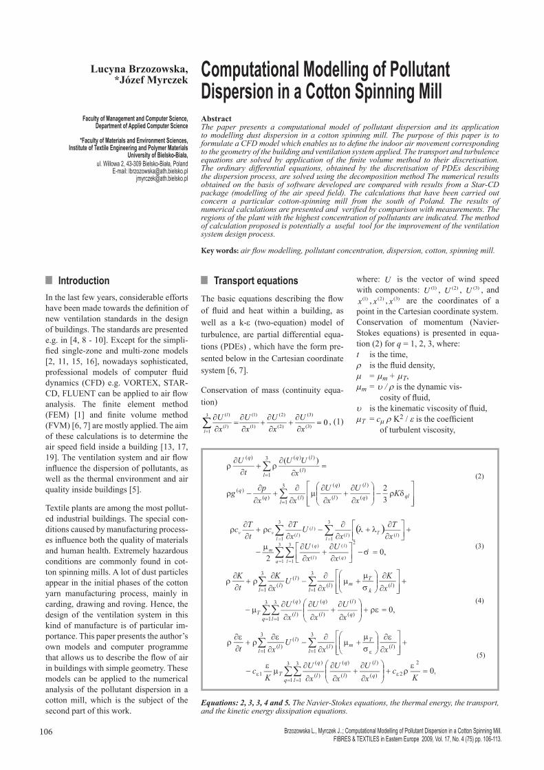
n Numerical solving of PDEsThe domain has the form of a rectangu-lar prism, shown in Figure 1. Air motion is created by a number of inlets in which the speed of air in the direction normal to the surface is defined, as well as the outlets ensuring the exchange of air.

Within the domain an element is distin-guished whose geometrical centre has the coordinates )3()2()1( ,, kji xxx .

Before defining its dimensions, we shall describe the general method of denoting points and elements.

If we investigate axis r, then, assuming that the length of the side of the domain in the direction r is L(r), the denotation presented in Figure 2 is used.

Interval ⟨0,L(r)⟩ is divided into nr subinter-vals with lengths )()(

1rn

rr

D÷D . In the centre of the subintervals points )()( r

nr

i rxx ÷ are

located. The ends of the subinterval, whose centre is )(r

ix , are denoted as)(

21

)(

21

r

i

r

ixx+−

÷ . Subintervals may be of equal

or different length.

The remaining equations, (1), (3), (4) and (5), are integrated over the volumes:

for i = 1, ..., n1, j = 1, ..., n2, k = 1, ..., n3.

In further considerations it is assumed that the boundary condition is one of the three following types.

Condition type W (Wall)Viscosity means that at the points where the air is in contact with a wall, the follow-ing conditions apply (no-slip conditions)

U(1) = 0, U(2) = 0, U(3)= 0 (6)

Figure 1. The domain investigated.

Figure 2. Denotation when dividing the interval ⟨0,L(r)⟩ into subintervals (r = 1, 2, 3).

FIBRES & TEXTILES in Eastern Europe 2009, Vol. 17, No. 5 (76)108

Condition type I (Inlet)Here it is assumed that the speed of air flowing in or out (in a direction normal to the wall) is known, and the other two components of speed are equal to zero. This means that in this case one of the following possibilities occurs

U(1) = U(1)(t), U(2) = 0, U(3)= 0 (7.1)U(2) = U(2)(t), U(1) = 0, U(3)= 0 (7.2)U(3) = U(3)(t), U(1) = 0, U(2)= 0 (7.3)

The aspects of conditions (7) used de-pends on which direction the wall is per-pendicular to.

Condition type O (Outlet)It is assumed that through the outlet in the wall, air flows in or out. In this case, it is generally assumed that

mkUxU k

m

m

≠==∂∂ for 0 ,0 )(

)(

)(

, (8.1)

pout = 0, (8.2)

where: m = 1, 2, 3 (according to the lo-

cation of the boundary),pout - pressure outside the domain (usu-

ally assumed to be equal to zero).

For boundaries with conditions of the outlet type, we formulate additional sim-plified differential equations which are solved together with other equations. Having used formulae given in detail in [6, 7], the equations for the problem after the discretisation step can be written in the form of

Navier-Stokes, energy and k-e equations:

U + g(U,T,K,E) + A . p = 0, (9.1)T + gT(U,T,K,E) = 0, (9.2)K + gK(U,T,K,E) = 0, (9.3)E + gE(U,T,K,E) = 0, (9.4)

Continuity equation:

B . U = h, (9.5)

where:A, B are matrices with constant coeffi-

cients, and U, p, T, K, E are vectors of unknowns in

the nodes described above.

The difficulty of solving Equations (9) is due to: 1. the non-linearity of Equation (9.1),2. vector p is not known while solving

Equation (9.1).

In this paper we use a procedure which en-ables Equations (9.1) to be integrated ac-cording to the Crank-Nicholson scheme. In order to determine vector p, we use an iterative procedure, which is a modifica-tion of the PISO algorithm [21, 22].

In order to perform the calculations, a computer program, called FV-mod, was written in Object Pascal (Delphi v. 7.0). This gave us an effective code, and hence calculations could be performed on an IBM PC. By using dynamic matrices, it is possible to perform calculations for several thousand elements. The program includes:n interactive input of data for calcula-

tions,

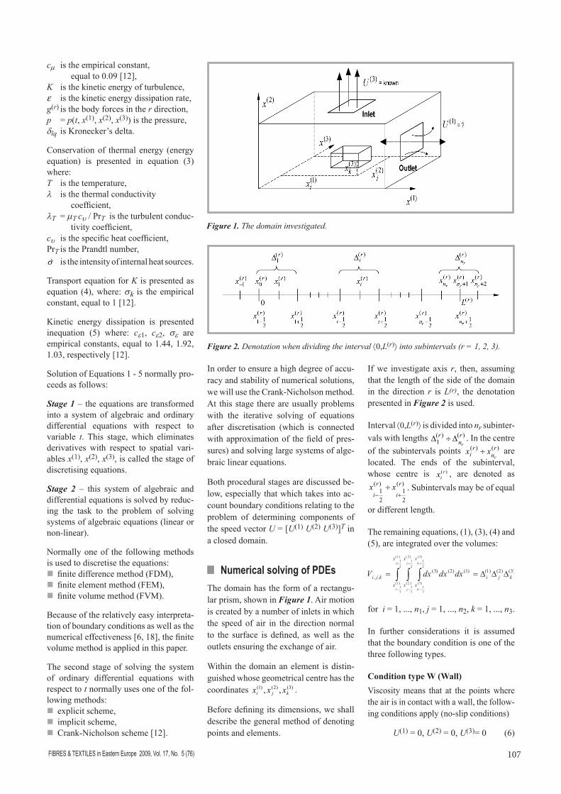
Figure 3. Model of the ventilation system in the spinning mill considered; A1 ÷ F1 – plenum (inlet) chambers, K1 ÷ K16 – inlet channels (ventilating ducts), I1 ÷ I64 – ventilators (Inlets), O1 ÷ O10 – ventilating holes (Outlets).

Table 1. Estimated data based on the real parameters of the spinning mill building acc. to Figure 3.

Chamber Efficiency of ventilators, m3/s Number of inlets Total area,

m2Air speed U(3),

m/sA1, A2 25.0 8 (I1 ÷ I8) 16 -1.56B1, B2 34.4 12 (I9 ÷ I20) 24 -1.44C1, C2 52.2 12 (I21 ÷ I32) 24 -2.18C3, C4 52.2 12 (I33 ÷ I44) 24 -2.18D1, D2 34.4 12 (I45 ÷ I56) 24 -1.44E1, F1 55.0 8 (I57 ÷ I64) 16 -3.44

Figure 4. Dimension of elements in x(2) direction: )2(,1, kiD = )2(

,54, kni +D = 1.5 m, )2(,24, kji −D = )2(

,4, kjiD

= 2 m, )2(,14, kji −D = 0.5 m, )2(

,14, kji +D = 2.5 m, j=1,…,15, )2(,2, kni +D = )2(

,4, kni +D = 2 m, )2(,3, kni +D = 0.5 m.

Figure 5. Percentage difference between the air velocity obtained by FV-mod and Star-CD.


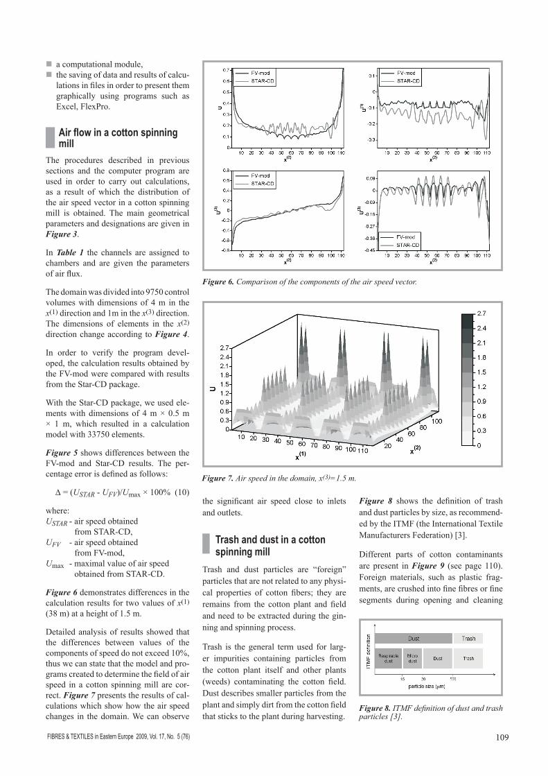
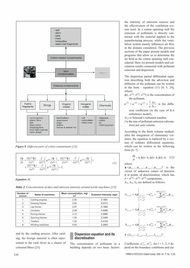
Figure 8 shows the definition of trash and dust particles by size, as recommend-ed by the ITMF (the International Textile Manufacturers Federation) [3].

Different parts of cotton contaminants are present in Figure 9 (see page 110). Foreign materials, such as plastic frag-ments, are crushed into fine fibres or fine segments during opening and cleaning

the significant air speed close to inlets and outlets.

Trash and dust in a cotton spinning mill

Trash and dust particles are “foreign” particles that are not related to any physi-cal properties of cotton fibers; they are remains from the cotton plant and field and need to be extracted during the gin-ning and spinning process.

Trash is the general term used for larg-er impurities containing particles from the cotton plant itself and other plants (weeds) contaminating the cotton field. Dust describes smaller particles from the plant and simply dirt from the cotton field that sticks to the plant during harvesting.

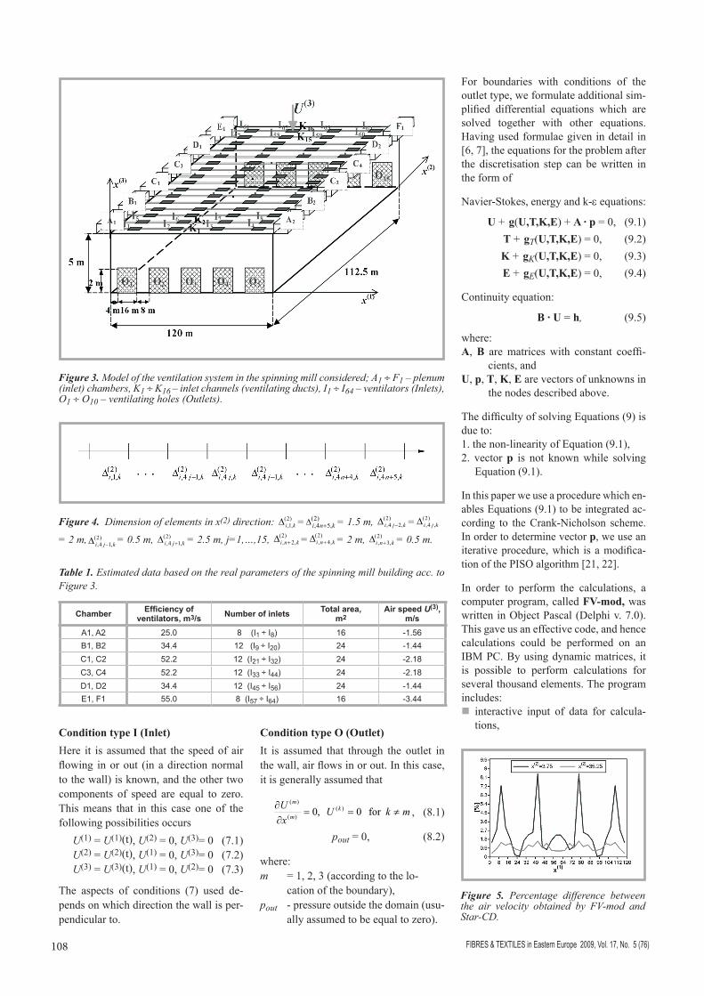
Figure 6. Comparison of the components of the air speed vector.

n a computational module,n the saving of data and results of calcu-

lations in files in order to present them graphically using programs such as Excel, FlexPro.

Air flow in a cotton spinning mill

The procedures described in previous sections and the computer program are used in order to carry out calculations, as a result of which the distribution of the air speed vector in a cotton spinning mill is obtained. The main geometrical parameters and designations are given in Figure 3.

In Table 1 the channels are assigned to chambers and are given the parameters of air flux.

The domain was divided into 9750 control volumes with dimensions of 4 m in the x(1) direction and 1m in the x(3) direction. The dimensions of elements in the x(2) direction change according to Figure 4.

In order to verify the program devel-oped, the calculation results obtained by the FV-mod were compared with results from the Star-CD package.

With the Star-CD package, we used ele-ments with dimensions of 4 m × 0.5 m × 1 m, which resulted in a calculation model with 33750 elements.

Figure 5 shows differences between the FV-mod and Star-CD results. The per-centage error is defined as follows:

D = (USTAR - UFV)/Umax × 100% (10)

where:USTAR - air speed obtained

from STAR-CD,UFV - air speed obtained

from FV-mod,Umax - maximal value of air speed

obtained from STAR-CD.

Figure 6 demonstrates differences in the calculation results for two values of x(1) (38 m) at a height of 1.5 m.

Detailed analysis of results showed that the differences between values of the components of speed do not exceed 10%, thus we can state that the model and pro-grams created to determine the field of air speed in a cotton spinning mill are cor-rect. Figure 7 presents the results of cal-culations which show how the air speed changes in the domain. We can observe

Figure 7. Air speed in the domain, x(3)=1.5 m.

Figure 8. ITMF definition of dust and trash particles [3].


Dispersion equation and its discretisation

The concentration of pollutants in a building depends on two basic factors:

the intensity of emission sources and the effectiveness of the ventilation sys-tem used. In a cotton spinning mill the emission of pollutants is directly con-nected with the material applied to the manufacturing process, while the venti-lation system mainly influences air flow in the domain considered. The previous sections of the paper present models and programs that allow us to determine the air field in the cotton spinning mill con-sidered. Here we present models and cal-culation results connected with pollutant emission and dispersion.

The dispersion partial differential equa-tion describing both the advection and diffusion of the pollutant can be written in the form - equation (11) [4, 5, 24], where: f(t, x(1), x(2), x(3)) is the concentration of

the pollutant,

is the diffu-

sion coefficient (in the case of K-e turbulence model),

ScT is Schmidt’s turbulent number,I is the rate of pollutant emission (absorp-

tion) per unit volume.

According to the finite volume method, after the integration of elementary vol-umes, the equation is replaced by a sys-tem of ordinary differential equations, which can be written in the following form [6, 7] :

, (12)

where: T

nnnkjin ],...,,...,,...,[3211 ,,,,1,1,1,1,1 ffff=f is the

vector of unknown values of function f at points of discretization, which has n = n(1) . n(2) . n(3) components,L1, L2, L3 are defined as follows:

∑+

−=

===

+==L},2min{

}1,2max{,,

)1(,,,

)1(,,1,,,1

)1(,

)3()3(

)2()2(

)1()1(

kj

k

j

i

ni

ilkjllkjikji

xxxxxxkji aA fαf

∑+

−=

===

+==L},2min{

}1,2max{,,

)2(,,,

)2(,,2,,,2

)2(,

)3()3(

)2()2(

)1()1(

ki

k

j

i

nj

jlklilkjikji

xxxxxxkji aA fαf

∑+

−=

===

+==L},2min{

}1,2max{,,

)3(,,,

)3(,,3,,,3

)3(,

)3()3(

)2()2(

)1()1(

ji

k

j

i

nk

klljilkjikji

xxxxxxkji aA fαf

T

nnnkjin IIII ],...,,...,,...,[3211 ,,,,1,1,1,1,1=f .

Coefficients )(,,

lkjia , )(

,,l

kjiα for l = 1, 2, 3 de-pend on the boundary conditions and sta-

and by the carding process. After card-ing, the foreign material is often repre-sented in the card sliver as a cluster of coloured fibres [23].

Figure 9. Different parts of cotton contaminants [23].

Table 2. Concentration of dust and emission intensity around textile machines [13].

Number of source Name of machines Mean concentration, mg/

m3 Emission intensity, mg/s

1 Carding engines 2.45 0.18812 Drawing frames 2.92 0.03133 Lap former 2.97 0.18604 Combers 2.56 0.00805 Roving frames 3.13 0.58856 Spinning frames 1.32 0.24907 Twisters 1.30 0.47458 Winding machines 0.83 0.2683

Equation 11.

(11)


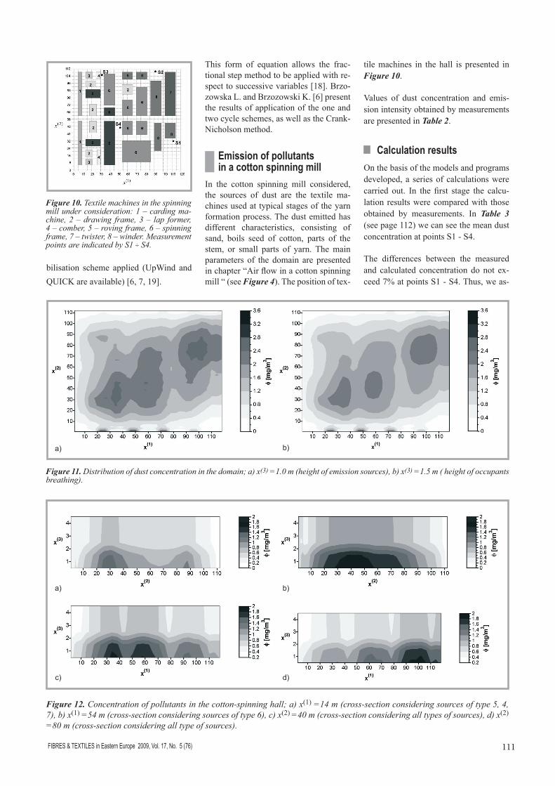
Figure 10. Textile machines in the spinning mill under consideration: 1 – carding ma-chine, 2 – drawing frame, 3 – lap former, 4 – comber, 5 – roving frame, 6 – spinning frame, 7 – twister, 8 – winder. Measurement points are indicated by S1 ÷ S4.

a) b)

Figure 11. Distribution of dust concentration in the domain; a) x(3) =1.0 m (height of emission sources), b) x(3) =1.5 m ( height of occupants breathing).

Figure 12. Concentration of pollutants in the cotton-spinning hall; a) x(1) =14 m (cross-section considering sources of type 5, 4, 7), b) x(1) =54 m (cross-section considering sources of type 6), c) x(2) =40 m (cross-section considering all types of sources), d) x(2) =80 m (cross-section considering all type of sources).

a) b)

c) d)

bilisation scheme applied (UpWind and QUICK are available) [6, 7, 19].

This form of equation allows the frac-tional step method to be applied with re-spect to successive variables [18]. Brzo-zowska L. and Brzozowski K. [6] present the results of application of the one and two cycle schemes, as well as the Crank-Nicholson method.

Emission of pollutants in a cotton spinning mill

In the cotton spinning mill considered, the sources of dust are the textile ma-chines used at typical stages of the yarn formation process. The dust emitted has different characteristics, consisting of sand, boils seed of cotton, parts of the stem, or small parts of yarn. The main parameters of the domain are presented in chapter “Air flow in a cotton spinning mill “ (see Figure 4). The position of tex-

tile machines in the hall is presented in Figure 10.

Values of dust concentration and emis-sion intensity obtained by measurements are presented in Table 2.

n Calculation resultsOn the basis of the models and programs developed, a series of calculations were carried out. In the first stage the calcu-lation results were compared with those obtained by measurements. In Table 3 (see page 112) we can see the mean dust concentration at points S1 - S4.

The differences between the measured and calculated concentration do not ex-ceed 7% at points S1 - S4. Thus, we as-


sume that the computer program gives correct results.

The concentrations of dust obtained at a height of 1.0 m and 1.5 m by calculations are presented in Figure 11.

Figure 12 shows how the concentration of pollutants changes with height x(3).

The maximal dust concentration can be observed in the environs of rowing ma-chines and twisters.

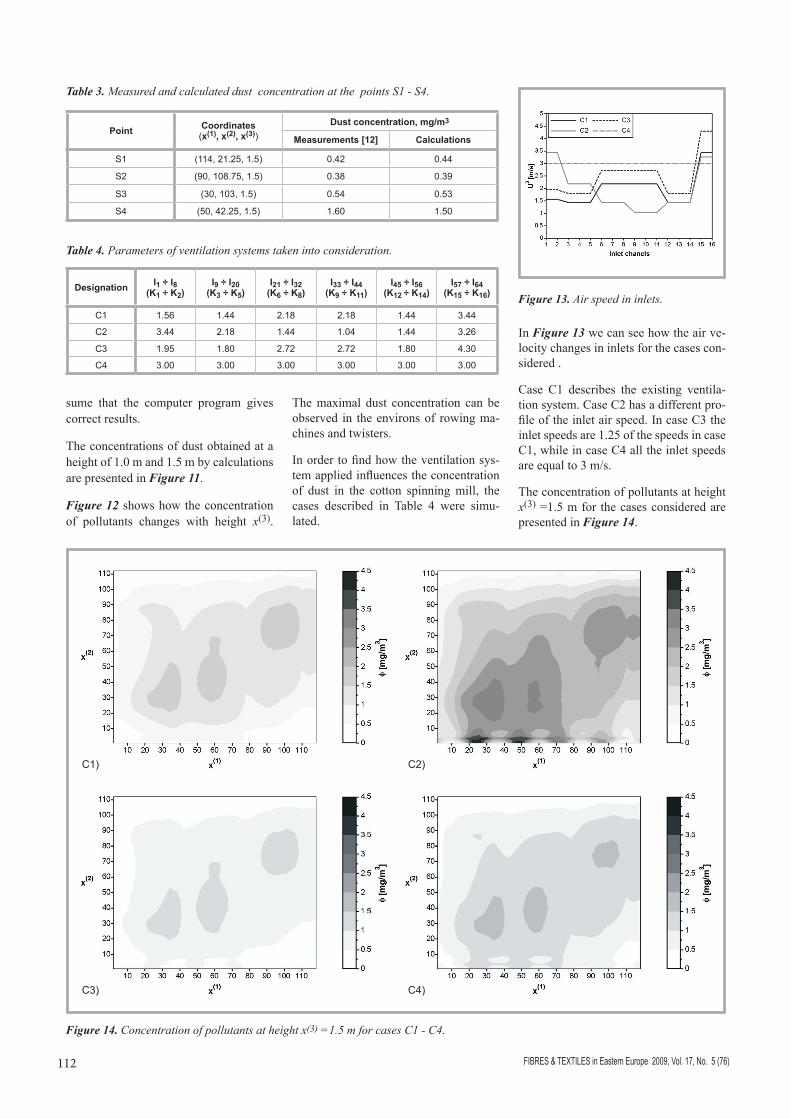
In order to find how the ventilation sys-tem applied influences the concentration of dust in the cotton spinning mill, the cases described in Table 4 were simu-lated.

In Figure 13 we can see how the air ve-locity changes in inlets for the cases con-sidered .

Case C1 describes the existing ventila-tion system. Case C2 has a different pro-file of the inlet air speed. In case C3 the inlet speeds are 1.25 of the speeds in case C1, while in case C4 all the inlet speeds are equal to 3 m/s.

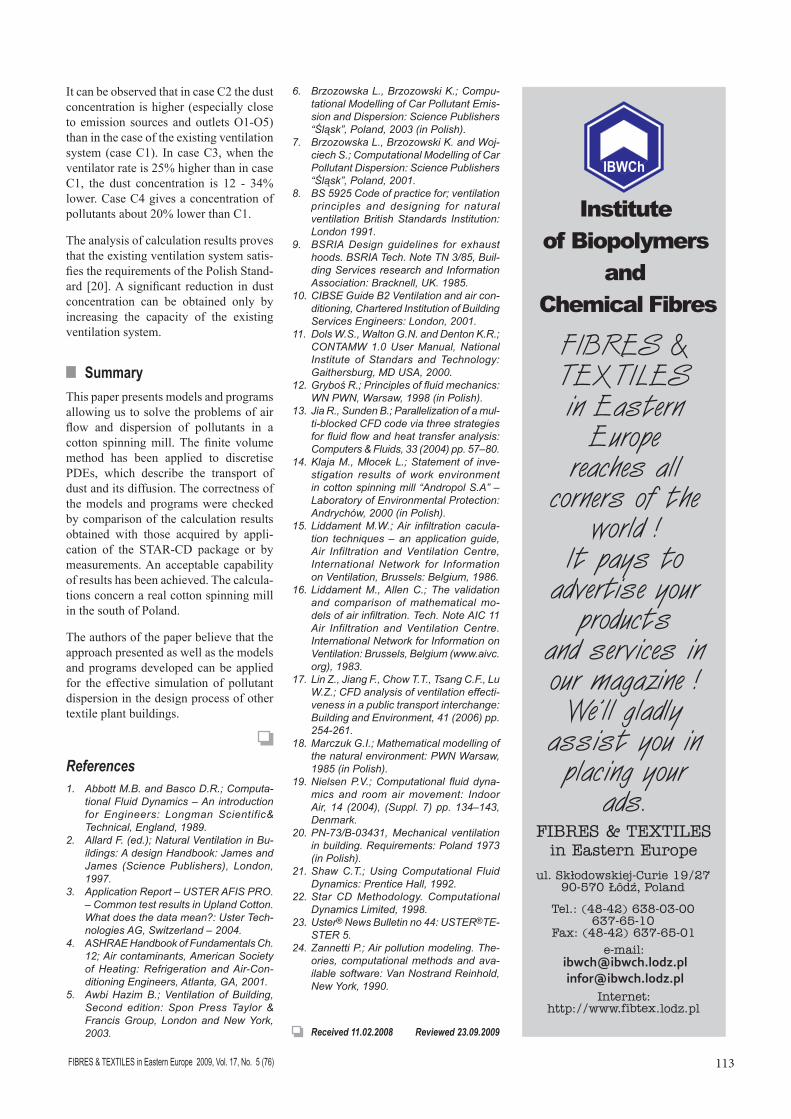
The concentration of pollutants at height x(3) =1.5 m for the cases considered are presented in Figure 14.

C1) C2)

C3) C4)

Figure 14. Concentration of pollutants at height x(3) =1.5 m for cases C1 - C4.

Figure 13. Air speed in inlets.

Table 4. Parameters of ventilation systems taken into consideration.

Designation I1 ÷ I8(K1 ÷ K2)

I9 ÷ I20(K3 ÷ K5)

I21 ÷ I32(K6 ÷ K8)

I33 ÷ I44(K9 ÷ K11)

I45 ÷ I56(K12 ÷ K14)

I57 ÷ I64(K15 ÷ K16)

C1 1.56 1.44 2.18 2.18 1.44 3.44

C2 3.44 2.18 1.44 1.04 1.44 3.26

C3 1.95 1.80 2.72 2.72 1.80 4.30

C4 3.00 3.00 3.00 3.00 3.00 3.00

Table 3. Measured and calculated dust concentration at the points S1 - S4.

Point Coordinates(x(1), x(2), x(3))

Dust concentration, mg/m3

Measurements [12] Calculations

S1 (114, 21.25, 1.5) 0.42 0.44

S2 (90, 108.75, 1.5) 0.38 0.39

S3 (30, 103, 1.5) 0.54 0.53

S4 (50, 42.25, 1.5) 1.60 1.50


Received 11.02.2008 Reviewed 23.09.2009

It can be observed that in case C2 the dust concentration is higher (especially close to emission sources and outlets O1-O5) than in the case of the existing ventilation system (case C1). In case C3, when the ventilator rate is 25% higher than in case C1, the dust concentration is 12 - 34% lower. Case C4 gives a concentration of pollutants about 20% lower than C1.

The analysis of calculation results proves that the existing ventilation system satis-fies the requirements of the Polish Stand-ard [20]. A significant reduction in dust concentration can be obtained only by increasing the capacity of the existing ventilation system.

n SummaryThis paper presents models and programs allowing us to solve the problems of air flow and dispersion of pollutants in a cotton spinning mill. The finite volume method has been applied to discretise PDEs, which describe the transport of dust and its diffusion. The correctness of the models and programs were checked by comparison of the calculation results obtained with those acquired by appli-cation of the STAR-CD package or by measurements. An acceptable capability of results has been achieved. The calcula-tions concern a real cotton spinning mill in the south of Poland.

The authors of the paper believe that the approach presented as well as the models and programs developed can be applied for the effective simulation of pollutant dispersion in the design process of other textile plant buildings.

References1. AbbottM.B.andBascoD.R.;Computa-

tionalFluidDynamics–Anintroductionfor Engineers: Longman Scientific&Technical,England,1989.

2. AllardF.(ed.);NaturalVentilationinBu-ildings:AdesignHandbook:JamesandJames (SciencePublishers), London,1997.

3. ApplicationReport–USTERAFISPRO.–CommontestresultsinUplandCotton.Whatdoesthedatamean?:UsterTech-nologiesAG,Switzerland–2004.

4. ASHRAEHandbookofFundamentalsCh.12;Aircontaminants,AmericanSocietyofHeating:Refrigeration andAir-Con-ditioningEngineers,Atlanta,GA,2001.

5. AwbiHazimB.;Ventilation ofBuilding,Second edition: SponPress Taylor &FrancisGroup, LondonandNewYork,2003.

6. BrzozowskaL.,BrzozowskiK.;Compu-tationalModellingofCarPollutantEmis-sionandDispersion:SciencePublishers“Śląsk”,Poland,2003(inPolish).

7. BrzozowskaL.,BrzozowskiK.andWoj-ciechS.;ComputationalModellingofCarPollutantDispersion:SciencePublishers“Śląsk”,Poland,2001.

8. BS5925Codeofpracticefor;ventilationprinciples and designing for naturalventilationBritishStandards Institution:London1991.

9. BSRIADesign guidelines for exhausthoods.BSRIATech.NoteTN3/85,Buil-dingServicesresearchandInformationAssociation:Bracknell,UK.1985.

10.CIBSEGuideB2Ventilationandaircon-ditioning,CharteredInstitutionofBuildingServicesEngineers:London,2001.

11. DolsW.S.,WaltonG.N.andDentonK.R.;CONTAMW1.0UserManual,NationalInstitute of Standars and Technology:Gaithersburg,MDUSA,2000.

12.GrybośR.;Principlesoffluidmechanics:WNPWN,Warsaw,1998(inPolish).

13.JiaR.,SundenB.;Parallelizationofamul-ti-blockedCFDcodeviathreestrategiesforfluidflowandheattransferanalysis:Computers&Fluids,33(2004)pp.57–80.

14.KlajaM.,MłocekL.;Statementof inve-stigation results of work environmentincottonspinningmill“AndropolS.A”–LaboratoryofEnvironmentalProtection:Andrychów,2000(inPolish).

15.LiddamentM.W.;Air infiltration cacula-tion techniques–anapplication guide,Air Infiltration and VentilationCentre,International Network for InformationonVentilation,Brussels:Belgium,1986.

16.LiddamentM.,AllenC.; The validationand comparison ofmathematicalmo-delsofairinfiltration.Tech.NoteAIC11Air Infiltration and VentilationCentre.InternationalNetworkforInformationonVentilation:Brussels,Belgium(www.aivc.org),1983.

17.LinZ.,JiangF.,ChowT.T.,TsangC.F.,LuW.Z.;CFDanalysisofventilationeffecti-venessinapublictransportinterchange:BuildingandEnvironment,41(2006)pp.254-261.

18.MarczukG.I.;Mathematicalmodellingofthenaturalenvironment:PWNWarsaw,1985(inPolish).

19.NielsenP.V.;Computational fluiddyna-mics and room airmovement: IndoorAir,14 (2004), (Suppl.7)pp.134–143,Denmark.

20.PN-73/B-03431,Mechanical ventilationinbuilding.Requirements:Poland1973(inPolish).

21.ShawC.T.;UsingComputational FluidDynamics:PrenticeHall,1992.

22.Star CDMethodology. ComputationalDynamicsLimited,1998.

23.Uster®NewsBulletinno44:USTER®TE-STER5.

24.ZannettiP.;Airpollutionmodeling.The-ories,computationalmethodsandava-ilablesoftware:VanNostrandReinhold,NewYork,1990.

Documents

Computational Modelling of Pollutant Dispersion in a