Calibrating pollutant dispersion in 1-D hydraulic models

HAL Id: hal-01118986https://hal.archives-ouvertes.fr/hal-01118986

Submitted on 20 Feb 2015

HAL is a multi-disciplinary open accessarchive for the deposit and dissemination of sci-entific research documents, whether they are pub-lished or not. The documents may come fromteaching and research institutions in France orabroad, or from public or private research centers.

L’archive ouverte pluridisciplinaire HAL, estdestinée au dépôt et à la diffusion de documentsscientifiques de niveau recherche, publiés ou non,émanant des établissements d’enseignement et derecherche français ou étrangers, des laboratoirespublics ou privés.

Calibrating pollutant dispersion in 1-D hydraulic modelsof river networks

M. Launay, J. Le Coz, B. Camenen, C. Walter, H. Angot, G. Dramais, J.B.Faure, Marina Coquery

To cite this version:M. Launay, J. Le Coz, B. Camenen, C. Walter, H. Angot, et al.. Calibrating pollutant dispersion in1-D hydraulic models of river networks. Journal of Hydro-environment Research, Elsevier, 2015, 9(1), pp.120-132. �10.1016/j.jher.2014.07.005�. �hal-01118986�

https://hal.archives-ouvertes.fr/hal-01118986

https://hal.archives-ouvertes.fr

Calibrating pollutant dispersion in 1-D hydraulic models of rivernetworks

M. Launaya, J. Le Coz∗,a, B. Camenena, C. Waltera, H. Angotb, G. Dramaisa, J.-B. Faurea, M. Coqueryb

aIrstea, UR HHLY, Hydrology-Hydraulics, 5 rue de la Doua - CS 70077 - F-69626 Villeurbanne, France.bIrstea, UR MALY, Freshwater Systems Ecology and Pollution, 5 rue de la Doua - CS 70077 - F-69626 Villeurbanne, France.

Abstract

The objective of this article is to investigate the major issues associated with the calibration of the pollu-tant dispersion in 1-D hydraulic models applied to river networks, especially large, complex, artificializedones where ecological and socio-economical threats are important. Such issues are illustrated and dis-cussed using the results of five fluorescent tracer experiments conducted in contrasted open-channel sys-tems, ranging from a simple trapezoidal canal to a more complex river network. Experimental dispersionvalues were quantified using both the change of moment method and a simple fit-by-eye procedure foreight river reaches with homogeneous hydraulic conditions and an achieved tracer mixing and dispersiveequilibrium. Since dispersion coefficient values depend on the assumed dispersion model, ideally theyshould be calibrated using the same model in which they are to be used, as was done in this study. Wealso derived concurrent longitudinal dispersion values using the velocity field measured by hydro-acousticprofilers (ADCP), which appears as a promising and cost-efficient technique for documenting dispersion inlarge river systems. It appears that the formulae for which the fit was mainly based on the cross-sectionalaspect ratio are generally more appropriate for field data than those which are sensitive to the velocity toshear velocity ratio. The interpretation of complex dispersion and mixing processes, along with the selec-tion of relevant dispersion coefficient predictors are key to minimizing errors in the numerical simulationof pollution dynamics in river networks.

Key words: longitudinal dispersion, river, pollution, 1-D hydraulic modelling, ADCP

1. Introduction

The pollution of rivers due to accidental spills represents a major threat to ecology and to various usesof water [33]. The environmental management of river systems requires accurate and efficient tools topredict pollutant concentration, propagation and dispersion, especially near water intakes when rivers areused as a source of drinking water [4]. A commonly used tool is numerical modelling, which is developedto simulate the hydraulic conditions and the transport and fate of solute or particulate pollutants along riversystems [17, 15, 36, 30].

At the river network scale, the application of two- and three-dimensional transport models is generallynot appropriate because of their time consuming computations [33] and because of the lack of data for theconstruction of such models and their validation. One-dimensional (1-D) transport models are generallypreferred for real-time predictions of the spatio-temporal dynamics of a pollution in large river networks.While simple, most 1-D models are able to simulate complex, multi-reach hydraulic networks, includingartificial structures as well as bifurcations and confluences.

In conventional 1-D hydraulic models, the transport of a fully mixed, passive pollutant or tracer is de-scribed by the 1-D advection-dispersion equation, also known as the Fickian model [40, 33]:

∂C∂t

+ U∂C∂x

= DL∂2C∂x2 (1)

∗Corresponding author. Tel: +33 472208786; fax: +33 478477875Email address: [email protected] (J. Le Coz)

Preprint submitted to Journal of Hydro-Environment Research December 19, 2014

Author-produced version of the article published in Journal of Hydro-environment Research (2015), vol. 9, issue 1, p. 120-132 The original publication is available at http://www.sciencedirect.com/ doi:10.1016/j.jher.2014.07.005

in which C is the section-averaged concentration, t the time, U the section-averaged velocity, x the distancein the longitudinal direction, and DL the longitudinal dispersion coefficient. The Fickian model for longi-tudinal dispersion applies when dispersive equilibrium is reached, i.e. when the effects of velocity shearare balanced by the effect of turbulent mixing [39]. Downstream of the injection point (or transverse line),this condition is achieved in the equilibrium zone, which establishes after the so-called advective zone.Equilibrium is reached when the tracer has sampled the entire flow, which generally occurs after the tracerconcentration is homogeneous throughout the cross-section. However, this is not a sufficient condition forchecking dispersion equilibrium.

In rivers and canals, longitudinal dispersion is mainly due to vertical and transverse velocity gradients,while molecular diffusion and turbulent diffusion are generally negligible. According to the literature, thelongitudinal dispersion varies within a range of 10−1 to 107 m2/s [20, 34, 27, 41], while the molecular andturbulent diffusion are in the order of 10−9 and 10−2 m2/s, respectively [39]. Note that turbulent diffusionmay vary from 10−3 to 1 m2/s, according to the hydraulic conditions. Usually, in rivers vertical velocitygradient effects on longitudinal dispersion are negligible compared to transverse velocity gradient effects[22]. It is therefore possible to accurately estimate longitudinal dispersion in natural streams from thetransverse velocity profile, as done by Seo and Baek [42] by fitting a beta function to the observed velocitydistribution.

Other mechanisms, such as trapping in recirculation zones, laminar boundary layers or porous media,can also cause dispersion. Such processes are usually designated as transient storage effects. Indeed, theobserved “tails” of breakthrough curves are often longer than can be accounted for by Eq. 1 applied ana-lytically to solute tracer pulses [37]. Hence, Bencala and Walters [5] introduced the effect of the transientstorage in the right-hand side of Eq. 1. Such model has been widely used to better understand physi-cal processes in experimental results (Cheong and Seo [12], Gooseff et al. [24], Worman and Wachniew[51], Bottacin-Busolin et al. [6], Szeftel et al. [48] among others). However, it remains difficult to beapplied in predictive models since it introduces two additional variables (solute concentration and cross-section area of the storage zone) and one additional parameter (stream storage exchange coefficient), whichmay be difficult to evaluate. Moreover, in large river cases dead-zones may be less relevant than in the smallrough streams studied in the literature focussing on transient storage mechanisms.

In 1-D hydraulic models, the longitudinal dispersion coefficient has to be predicted through formulaeaccounting for the mainstream longitudinal dispersion, usually ignoring the transient storage effects thatwere highlighted by research in the last decades [39]. Such semi-empirical formulae were establishedagainst experimental data sets to relate the longitudinal dispersion coefficient to the bulk characteristics ofthe flow. However, the predictive accuracy of such formulae is often questionable, which can be explainedby the scatter and lack of representativeness of the underlying data set.

Soluble tracer experiments are the most direct method to collect field data on longitudinal dispersion inrivers [26]. Passive tracers injected into a stream behave in the same way as conservative pollutants andtheir monitoring is feasible using either in-situ recording instruments or water samples to be analysed inthe laboratory. An ideal tracer should be readily water soluble, easily detectable, harmless at low concen-trations, stable, and inexpensive [13, 50, 18]. However, field data remain scarce in large river networks,mainly due to the logistical difficulty and the high cost of tracing operations. Most large-scale river tracertests were performed in the 1960s and 1970s [50]. Among recent studies at a large scale (i.e. at least 10 kmlength), those performed on the Hudson River, USA [25, 8], in several Portuguese rivers [15] and on theNarew River, Poland [38] should be mentioned.

In recent years, some authors [9, 43, 31] used ADCP data in order to compute the longitudinal shear-driven dispersion at a cross-section of a river. For two decades indeed, acoustic Doppler current profilers(ADCP) have been increasingly used by hydrometric services to efficiently measure discharge in rivers.The most common procedure is the mobile-boat method for which the vessel-mounted ADCP scans bothflow depth and velocity field during a crossing of the river section. While the derivation of longitudinaldispersion from the velocity field throughout a cross-section was known for long [22], velocity samplingby ADCP offers an attractive and cost-efficient solution for measuring dispersion in rivers, especially in thelargest ones.

The objective of this article is to investigate the major issues associated with the calibration of pollu-tant dispersion in 1-D hydraulic models applied to river networks, especially large, complex, artificializedones where ecological and socio-economical threats are important. From the modeller’s standpoint, the

2


Table 1: Values of the parameters in empirical formulas for the estimation of longitudinal dispersion coefficient (Eq. 2)

Authors a b c

Elder [16] 5.93 0 0Fischer [21] 0.011 2 2Liu [34] 0.18 0.5 2Iwasa and Aya [27] 2 0 1.5Seo and Cheong [41] 5.915 1.428 0.62Koussis and Rodriguez-Mirasol [32] 0.6 0 2

major questions are the following: Is most of the pollutant fully mixed and is the dispersive equilibriumreached so that the Fickian model applies? Are transient storage effects negligible or would they requirethe consideration of additional terms? How accurate are the dispersion coefficient values predicted by con-ventional formulae, and how sensitive are the modelling results to the choice of a formula? Such issuesare illustrated and discussed using the results of new, comprehensive fluorescent tracer experiments, withconcurrent ADCP-based velocity surveys and dispersion estimation.

2. Longitudinal dispersion in 1-D river models

2.1. Numerical simulation toolsIn this study, the river systems were simulated using Mage, a typical 1-D loop-meshed hydrodynamic

code [46] with AdisTS, an advection-dispersion resolution for pollutant and suspended-sediment transport[1]. Mage is a 1-D hydrodynamic model simulating flow in transient regime. The 1-D Barre de Saint-Venant equations (shallow water equations) are solved using a four point finite difference scheme. Thereal geometry of the river bed is represented by a set of cross-sections that is used for the calculation. Thenetwork topology may be looped to represent islands or multi-branched networks with confluences andbifurcations. This model presents very low computation times, which allow for real-time simulation orsimulation of long time series [1]. The partitioning of discharges at bifurcations is governed either by thegeometry of the river bed or by the representation of flow controlling structures such as dams.

AdisTS solves the Fickian model (Eq. 1), using a numerical resolution of the advection-dispersion equa-tion which is based on operator splitting. The advection part is solved using a TVD scheme (Total VariationDiminishing) with the Superbee flux limiter and is adapted to non uniform space steps. This scheme is wellknown to dramatically reduce the numerical dispersion. AdisTS allows the user either to set a fixed valuefor DL or to use a predictive formula, by setting the a, b, and c calibration parameters of the followingequation:

DL

HU∗= a

(UU∗

)b (WH

)c

(2)

where W is the river width, H is the section-averaged water depth, U∗ =√τ/ρ is the shear velocity, τ the

section-averaged bed shear stress, ρ the water density. Different authors have established numerous empir-ical formulae of this type, based on a dimensional analysis of the dispersion coefficient. Since longitudinaldispersion in open channels is mainly driven by velocity gradients and turbulent mixing, the main controlfactors are the U/U∗ ratio, which captures turbulent shear intensity, and the W/H aspect ratio, which cap-tures the transversal velocity gradient and the secondary currents intensity. The different authors suggestedcontrasted values for parameters a, b, and c as presented in Table 1. From the following review of theliterature, it is a relevant question whether conventional formulae do accurately predict the real Fickiandispersion coefficient values, especially in large river systems.

2.2. Review of predictive formulae used in 1-D modelsMost of the authors who suggested an empirical formula in the form of Eq. 2 used a very similar data set.

Seo and Cheong [41] gave a listing of these data, which mainly correspond to measurements in US rivers3


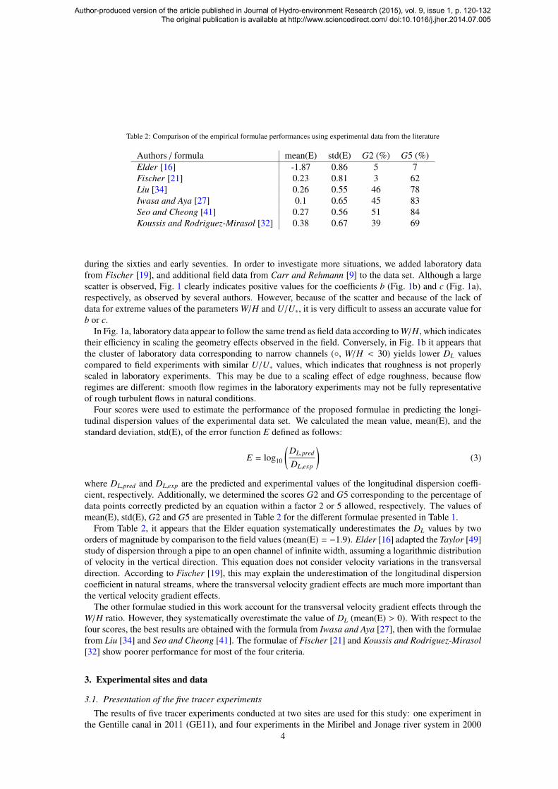
Table 2: Comparison of the empirical formulae performances using experimental data from the literature

Authors / formula mean(E) std(E) G2 (%) G5 (%)Elder [16] -1.87 0.86 5 7Fischer [21] 0.23 0.81 3 62Liu [34] 0.26 0.55 46 78Iwasa and Aya [27] 0.1 0.65 45 83Seo and Cheong [41] 0.27 0.56 51 84Koussis and Rodriguez-Mirasol [32] 0.38 0.67 39 69

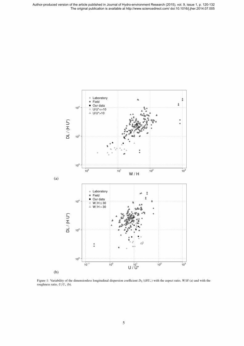
during the sixties and early seventies. In order to investigate more situations, we added laboratory datafrom Fischer [19], and additional field data from Carr and Rehmann [9] to the data set. Although a largescatter is observed, Fig. 1 clearly indicates positive values for the coefficients b (Fig. 1b) and c (Fig. 1a),respectively, as observed by several authors. However, because of the scatter and because of the lack ofdata for extreme values of the parameters W/H and U/U∗, it is very difficult to assess an accurate value forb or c.

In Fig. 1a, laboratory data appear to follow the same trend as field data according to W/H, which indicatestheir efficiency in scaling the geometry effects observed in the field. Conversely, in Fig. 1b it appears thatthe cluster of laboratory data corresponding to narrow channels (◦, W/H < 30) yields lower DL valuescompared to field experiments with similar U/U∗ values, which indicates that roughness is not properlyscaled in laboratory experiments. This may be due to a scaling effect of edge roughness, because flowregimes are different: smooth flow regimes in the laboratory experiments may not be fully representativeof rough turbulent flows in natural conditions.

Four scores were used to estimate the performance of the proposed formulae in predicting the longi-tudinal dispersion values of the experimental data set. We calculated the mean value, mean(E), and thestandard deviation, std(E), of the error function E defined as follows:

E = log10

(DL,pred

DL,exp

)(3)

where DL,pred and DL,exp are the predicted and experimental values of the longitudinal dispersion coeffi-cient, respectively. Additionally, we determined the scores G2 and G5 corresponding to the percentage ofdata points correctly predicted by an equation within a factor 2 or 5 allowed, respectively. The values ofmean(E), std(E), G2 and G5 are presented in Table 2 for the different formulae presented in Table 1.

From Table 2, it appears that the Elder equation systematically underestimates the DL values by twoorders of magnitude by comparison to the field values (mean(E) = −1.9). Elder [16] adapted the Taylor [49]study of dispersion through a pipe to an open channel of infinite width, assuming a logarithmic distributionof velocity in the vertical direction. This equation does not consider velocity variations in the transversaldirection. According to Fischer [19], this may explain the underestimation of the longitudinal dispersioncoefficient in natural streams, where the transversal velocity gradient effects are much more important thanthe vertical velocity gradient effects.

The other formulae studied in this work account for the transversal velocity gradient effects through theW/H ratio. However, they systematically overestimate the value of DL (mean(E) > 0). With respect to thefour scores, the best results are obtained with the formula from Iwasa and Aya [27], then with the formulaefrom Liu [34] and Seo and Cheong [41]. The formulae of Fischer [21] and Koussis and Rodriguez-Mirasol[32] show poorer performance for most of the four criteria.

3. Experimental sites and data

3.1. Presentation of the five tracer experiments

The results of five tracer experiments conducted at two sites are used for this study: one experiment inthe Gentille canal in 2011 (GE11), and four experiments in the Miribel and Jonage river system in 2000

4


(a)

100 101 102 103

100

102

104

W / H

DL

/(H

U*)

LaboratoryFieldOur dataU/U*<=10U/U*>10

(b)

10−1 100 101 102 103

100

102

104

U / U*

DL

/(H

U*)

LaboratoryFieldOur dataW H ≤ 30W H > 30

Figure 1: Variability of the dimensionless longitudinal dispersion coefficient DL/(HU∗) with the aspect ratio, W/H (a) and with theroughness ratio, U/U∗ (b).

5


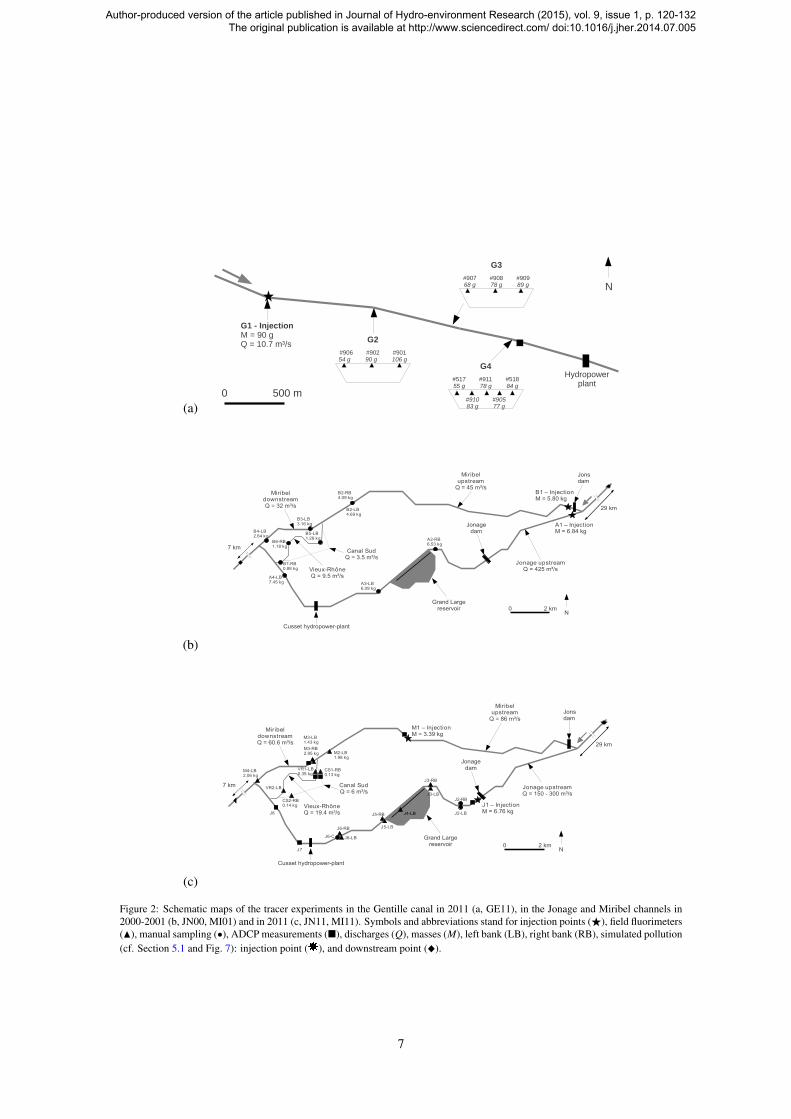
(JN00), 2001 (MI01), and 2011 (JN11, MI11). Experimental conditions for the five tracer experiments aresummarized in the maps of the experimental sites in Fig. 2, and further details for each experiment areprovided in the following paragraphs.

In all experiments, Rhodamine was used as a fluorescent tracer, which is considered as an efficient tracerfor large open-channel flows [45]. Whereas Rhodamine B was used in 2000 and 2001 tracer experiments,we preferred Rhodamine WT in 2011 since it is considered much less toxic. Except for the 2000-2001experiments for which only water sampling was performed to monitor tracer concentrations, the concen-tration was monitored in situ using several field fluorimeters (Albillia FL30 GGUN) and one fluorimeterin the laboratory (Datalink FL200-R). Field fluorimeters allow for a continuous recording of the river fluo-rescence level but their quantification limits are poorer (4 µg/L) than those of laboratory devices (1 µg/L).Water sampling and the slightly postponed analysis in the laboratory provided accurate data to calibrate thecontinuous monitoring by field fluorimeters.

The Gentille Canal (Fig. 2a) is a 14 m wide, 2 m deep concrete canal for a hydropower plant on theGaronne River, France. It differs in scale and complexity from the other experimental site. This 2 km long,trapezoidal canal was used to compare tracer experiments conducted in large rivers with results from asmaller scale stream, with a prismatic geometry and smooth bed and walls. During the tracer experiment,the flow was nearly uniform over the whole reach, and the discharge continuously recorded by ADCP wasnearly constant. Rhodamine WT was injected as a slug in the centre of the cross-section. Three to fivefluorimeters were hung from bridges and immersed approximately 50 cm below the surface in order tomonitor the lateral mixing of the tracer, as well as its longitudinal propagation and dispersion.

The Miribel and Jonage river system (Fig. 2b and c) is an artificialized section of the Rhone Riverupstream of Lyon, France. The Miribel and Jonage canals were built in the anastomosing system of theRhone River during the XIXth century. Only a small stretch of the former river bed is remaining, which iscalled Vieux-Rhone. The bed of these reaches is mainly composed of coarse sediments (grain size varyingfrom 5 to 10 cm). Several structures were built for hydropower purpose: Jons dam on the Miribel canal,which in normal hydrological conditions deviates most of the flow to the Jonage canal, and Jonage damand Cusset hydropower plant situated on the Jonage canal. The Grand Large lake is located along theJonage canal but a wall made of sheet pile prevents exchanges between the canal and the reservoir. Visualinspection and sampling survey during the experiment confirmed that tracer concentrations in the lake werenegligible.

First experiments had been conducted by others in the Miribel and Jonage system in 2001 (Miribel)and in 2000 (Jonage). Unfortunately, the discharge was not continuously recorded within the traced riverbranches. The discharge in the Miribel channel was claimed to be 30 m3/s by the dam managers, whichmay be underestimated based on our recent direct observations for similar conditions.

The fluorescent tracer Rhodamine B was injected continuously from a bank during one hour at a constantrate, in the vicinity of Jons dam. Manual samples were taken at a limited number of sites as shown inFig. 2b, for subsequent laboratory analysis of their fluorescence. In spite of the rather poor temporalresolution, the collected data provide valuable indications on the dispersion processes. to determine thedispersion coefficient.

During the experiments conducted in 2011 in Miribel and Jonage channels, the discharges were moni-tored continuously using vessel-mounted ADCP set up on boats. Discharge was measured at the injectionpoint, at each bifurcation and at the downstream end of hydraulically homogeneous reaches, with a typicaluncertainty of 5%. Discharge in Miribel channel remained constant over the experiment period, whereasdischarge in Jonage channel increased from 150 m3/s to almost 300 m3/s. The injection into the Miribelcanal was achieved 6 to 7 km further downstream than the 2000-2001 injections, and the injection pointfor the Jonage canal was located just downstream of the Jonage dam. For these two experiments, thefluorescent tracer Rhodamine WT was injected from a boat as a slug distributed over a transect line.

Field fluorimeters were either hung from bridges and immersed at mid-depth, or set up from banks onthe river bed, as far from the bank as possible. At some monitoring points, two or three fluorimeterswere set up at different positions within the same cross-section, in order to verify the complete mixing oftracer across the section. Water sampling was performed either from banks or bridges using plastic bucketsor automatic samplers. The sampling frequency was every 10 minutes during the peak concentration andevery 30 minutes before and after the peak. The water samples were stored in plastic bottles and transportedimmediately to the laboratory to be analysed using the laboratory fluorimeter. Specific attention was paid

6


(a)0 500 m

N

G1 - InjectionM = 90 gQ = 10.7 m³/s G2

#906 #902 #90154 g 90 g 106 g

G3

#907 #908 #90968 g 78 g 89 g

G4

#517 #911 #51855 g 78 g 84 g

#910 #90583 g 77 g

Hydropower plant

(b)

BRC–CInjectionMC=CG/8xCkg

JonsCdam

ARC–CInjectionMC=Cv/8SCkg

CussetChydropower³plant

x ôCkm

Bô³LBS/v9Ckg

MiribelCdownstreamQC=CNôCm³Vs

Vieux³RhôneQC=C9/GCm³Vs

N

CanalCSudQC=CN/GCm³Vs

MiribelCupstream

QC=CSGCm³Vs

JonageCupstreamQC=CSôGCm³Vs

JonageCdam

GrandCLargeCreservoir

Bô³RBS/x9Ckg

BN³LBN/RvCkg

BS³LBô/vSCkg

BG³LBR/ôvCkg

Bv³RBR/R8Ckg

B7³RBx/88Ckg

AS³LB7/SGCkg AN³LB

v/x9Ckg

Aô³RBv/GNCkg

ô9Ckm

7Ckm

(c)

Môy–yInjectionMy=y5/59ykg

Jonsydam

Jôy–yInjectionMy=y6/76ykg

J5³RB

Cussetyhydropower³plant

x Nykm

MG³LBN/x6ykg

M5³LBô/G5ykg

MN³LBô/98ykg

CSô³RBx/ô5ykg

MiribelydownstreamQy=y6x/6ym³Vs

Vieux³RhôneQy=yô9/Gym³Vs

N

CanalySudQy=y6ym³Vs

JN³LB

JN³RBJ5³LB

Jv³RB

Jv³LB

JG³LB

J6³RB

J6³LBJ6³C

J7

J8

M5³RBN/9vykg

CSN³RBx/ôGykg

VRN³LB

VRô³LBx/5vykg

Miribelyupstream

Qy=y86ym³Vs

JonageyupstreamQy=yôvxy³y5xxym³Vs

Jonageydam

GrandyLargeyreservoir

N9ykm

7ykm

Figure 2: Schematic maps of the tracer experiments in the Gentille canal in 2011 (a, GE11), in the Jonage and Miribel channels in2000-2001 (b, JN00, MI01) and in 2011 (c, JN11, MI11). Symbols and abbreviations stand for injection points (F), field fluorimeters(N), manual sampling (•), ADCP measurements (�), discharges (Q), masses (M), left bank (LB), right bank (RB), simulated pollution(cf. Section 5.1 and Fig. 7): injection point (I), and downstream point (_).

7


to the transport and storage of samples in order to minimize potential variations of the water characteristics(temperature, light exposure).

3.2. Assessment of the equilibrium zones

The breakthrough curves for all the 2011 experiments differ from pure Gaussian curves, especially inthat they are skewed (Fig. 3), which had to be expected. Indeed, Rutherford [39] acknowledged thatbreakthrough curves recorded from laboratory or field experiments are actually never found to be Gaussian.He further explained that this is not only due to transient storage effects by dead zones and laminar near-bedlayers, but also notably due to the skewness induced by the propagation of the non-mixed tracer along theadvective zone, between the source cross-section and the equilibrium zone.

From our observations downstream of the injection points, and in the absence of significant dead zonesor hyporheic flows, the advective effects are the most realistic cause for the skewed breakthrough curves inour tracer experiments.

As explained in the introduction, the Fickian model (Eq. 1) used in most 1-D models applies in the equi-librium zone, downstream of the advective zone. The length of the advective zone, Lx, may be estimatedusing the following formula [22, 39]:

Lx = αUL2

t

Dy(4)

with α =0.3-0.6 in smooth channels, and α =1-5 and even more for rough, small channels. Lt is the distancefrom the maximum velocity point to the nearest bank, and Dy is the transverse dispersion coefficient.Following Rutherford [39], we will consider that Lt =0.5-0.7W and that Dy =0.3-0.9HU∗ for irregular butonly gently meandering natural channels. We also assume that α ≈ 1.

The assessment of the advective zone length (Eq. 4), along with verification of the tracer mixing andmass continuity (see e.g. Jobson [28]), will be further used to identify the river reaches where reliablelongitudinal dispersion values can be derived from our tracing results. According to Hubbard et al. [26],the transversal and vertical mixing is complete if the areas of the time-concentration curves observed atdifferent points in the cross-section are the same. Differences across a river section in the times of peakconcentration and in the shapes of breakthrough curves also provide information on mixing and equilib-rium.

3.3. Review of the exploitable tracing results

Eight reaches (see Table 4) were selected where hydraulic conditions were found to be nearly uniform,and where sufficient mixing and tracer equilibrium were checked, according to the methods described inthe previous section. Fig. 2 presents the masses computed from the concentration curves recorded by eachfluorimeter for all tracer experiments. The Lx distances computed with Eq. 4 are also reported in Table 4.

In the Gentille canal, the distances between the injection point and the sampling positions are greaterthan Lx, which suggests that dispersive equilibrium should be acceptably achieved in this canal. However,the concentrations recorded on the right part of the flow remained slightly higher than on the left part at allmonitoring stations along the reach (Fig. 3a).

Full mixing was more questionable in the Miribel canal experiments. In 2001, the distance from theinjection position B1 to the bifurcation B2 between the Miribel canal and the Vieux-Rhone stream (Fig. 2b)is slightly larger than Lx. It can therefore be reasonably assumed that mixing was at least partially reached,though not totally. The difference between the injected mass and that recorded at B2 may be explained bythe uncertainty in the discharge claimed by the dam manager and used for the calculation.

While mass continuity is observed in 2001 at the bifurcation between Miribel canal and the Vieux-Rhone, the masses recorded in 2011 at M3-LB and M3-RB are not equivalent (see Fig. 2c). The break-through curves along Miribel channel (Fig. 3b) show different shapes and times of the peak concentration,according to the measurement positions. This is consistent with the fact that in 2011 the distance betweenthe injection point and the bifurcation was shorter than in 2001, and smaller than Lx. Experimental data inthe downstream part of Miribel channel in 2011 should therefore be interpreted carefully, considering theincomplete transversal mixing at M3.

Based on the comparison of tracer masses, full mixing seems to be achieved in the Vieux-Rhone in 2001(Fig. 2b) and in the Vieux-Rhone and Canal Sud area for the 2011 experiments (Fig. 2b and Fig. 3c). The

8


13:30 14:00 14:30 15:00 15:301,0E-6

3,0E-6

5,0E-6

7,0E-6

9,0E-6

1,1E-5

1,3E-5

Gentille 2011

G2_LB G3_LB G4_LBG2_M G3_M G4_MG2_RB G3_RB G4_RB

Co

nc

en

trat

ion

(g

/L)

1.3.10-5

9.10-6

5.10-6

1.10-6

3.10-6

7.10-6

1.1.10-5

1.10-6

6.10-6

1.10-6

1.1.10-5

1.6.10-5

5

9

13

Co

nce

ntr

atio

n (

µg

/L)

114:00 14:30 15:00 15:30

Time (h)13:30

Gentille 2011

11

7

3

09:00 10:00 11:00 12:00 13:00 14:001,0E-6

6,0E-6

1,1E-5

1,6E-5

2,1E-5

2,6E-5

Miribel 2011

M2_LB M3_LB

M3_RB M4_LB

Co

nc

en

tra

tio

n (g

/L)

1.10-6

6.10-6

1.1.10-5

1.6.10-5

2.1.10-5

2.6.10-6

1.10-6

6.10-6

1.10-6

1.1.10-5

1.6.10-5

6

16

26

Co

nc

entr

atio

n (

µg

/L)

110 11 12 13 14

Time (h)9

Miribel 2011

21

11

(a) (b)

09:00 10:00 11:00 12:00 13:00 14:001,0E-6

6,0E-6

1,1E-5

1,6E-5

Vieux-Rhône / Canal Sud 2011

M2_LB VR1_LB

CS1_RB CS2_RB

Co

nc

en

tra

tio

n (

g/L

)

1.10-6

6.10-6

1.10-6

1.1.10-5

1.6.10-5

6

11

16

Co

nce

ntr

atio

n (

µg

/L)

110 11 12 13 14

Time (h)9

Vieux Rhône / Canal Sud 2011

09:00 10:00 11:00 12:00 13:00 14:00 15:00 16:00 17:001,0E-6

6,0E-6

1,1E-5

1,6E-5

2,1E-5

2,6E-5

3,1E-5Jonage 2011

J2_LB J3_LB J5_LB J6_LB J6_MJ2_RB J3_RB J5_RB J6_RB

Co

nc

entr

atio

n (g

/L)

J2_LB J3_LB J5_LB J6_LB J6_MJ2_RB J3_RB J5_RB J6_RB

1.10-6

6.10-6

1.1.10-5

1.6.10-5

2.1.10-5

2.6.10-5

3.1.10-5

1.10-6

6.10-6

1.10-6

1.1.10-5

1.6.10-5

6

11

16

Co

nce

ntr

atio

n (

µg

/L)

10 11 12 13 14Time (h)

9

Jonage 2011

15 16 171

21

26

31

(c) (d)

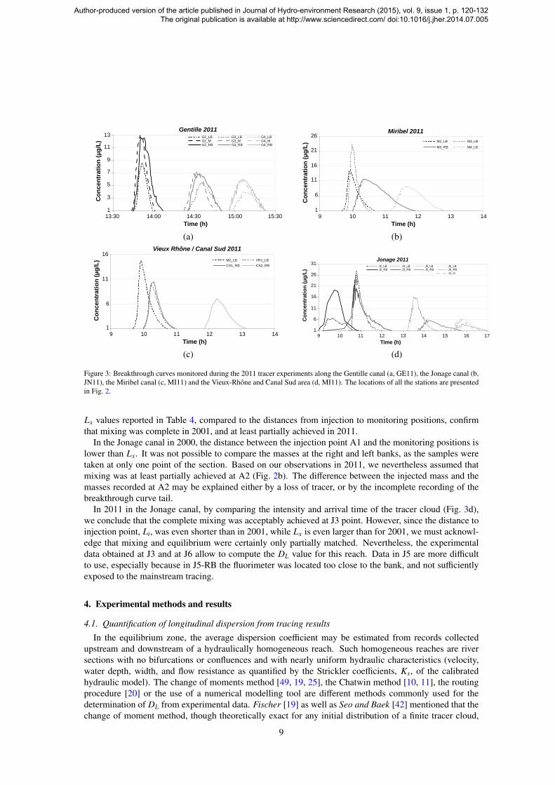
Figure 3: Breakthrough curves monitored during the 2011 tracer experiments along the Gentille canal (a, GE11), the Jonage canal (b,JN11), the Miribel canal (c, MI11) and the Vieux-Rhone and Canal Sud area (d, MI11). The locations of all the stations are presentedin Fig. 2.

Lx values reported in Table 4, compared to the distances from injection to monitoring positions, confirmthat mixing was complete in 2001, and at least partially achieved in 2011.

In the Jonage canal in 2000, the distance between the injection point A1 and the monitoring positions islower than Lx. It was not possible to compare the masses at the right and left banks, as the samples weretaken at only one point of the section. Based on our observations in 2011, we nevertheless assumed thatmixing was at least partially achieved at A2 (Fig. 2b). The difference between the injected mass and themasses recorded at A2 may be explained either by a loss of tracer, or by the incomplete recording of thebreakthrough curve tail.

In 2011 in the Jonage canal, by comparing the intensity and arrival time of the tracer cloud (Fig. 3d),we conclude that the complete mixing was acceptably achieved at J3 point. However, since the distance toinjection point, Li, was even shorter than in 2001, while Lx is even larger than for 2001, we must acknowl-edge that mixing and equilibrium were certainly only partially matched. Nevertheless, the experimentaldata obtained at J3 and at J6 allow to compute the DL value for this reach. Data in J5 are more difficultto use, especially because in J5-RB the fluorimeter was located too close to the bank, and not sufficientlyexposed to the mainstream tracing.

4. Experimental methods and results

4.1. Quantification of longitudinal dispersion from tracing results

In the equilibrium zone, the average dispersion coefficient may be estimated from records collectedupstream and downstream of a hydraulically homogeneous reach. Such homogeneous reaches are riversections with no bifurcations or confluences and with nearly uniform hydraulic characteristics (velocity,water depth, width, and flow resistance as quantified by the Strickler coefficients, Ks, of the calibratedhydraulic model). The change of moments method [49, 19, 25], the Chatwin method [10, 11], the routingprocedure [20] or the use of a numerical modelling tool are different methods commonly used for thedetermination of DL from experimental data. Fischer [19] as well as Seo and Baek [42] mentioned that thechange of moment method, though theoretically exact for any initial distribution of a finite tracer cloud,

9


13,5 14 14,5 15 15,5 16

1,0E-6

6,0E-6

1,1E-5

1,6E-516

11

6

Co

nce

ntr

atio

n (

µg

/L)

13:30 14:00 14:30 15:00 15:30

Time16:00

1

Observed Simulated D

L = 0.12 m²/s

Simulated DL = 1.2 m²/s

Simulated DL = 12 m²/s

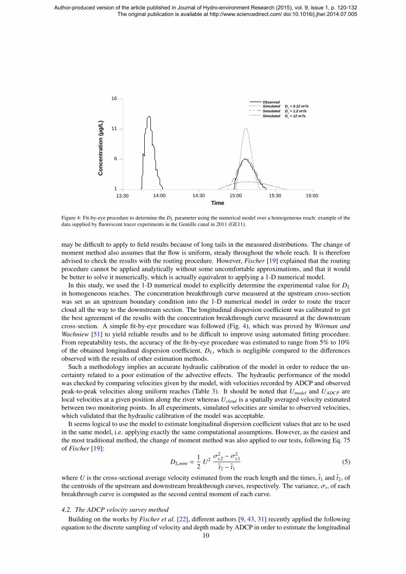
Figure 4: Fit-by-eye procedure to determine the DL parameter using the numerical model over a homogeneous reach: example of thedata supplied by fluorescent tracer experiments in the Gentille canal in 2011 (GE11).

may be difficult to apply to field results because of long tails in the measured distributions. The change ofmoment method also assumes that the flow is uniform, steady throughout the whole reach. It is thereforeadvised to check the results with the routing procedure. However, Fischer [19] explained that the routingprocedure cannot be applied analytically without some uncomfortable approximations, and that it wouldbe better to solve it numerically, which is actually equivalent to applying a 1-D numerical model.

In this study, we used the 1-D numerical model to explicitly determine the experimental value for DL

in homogeneous reaches. The concentration breakthrough curve measured at the upstream cross-sectionwas set as an upstream boundary condition into the 1-D numerical model in order to route the tracercloud all the way to the downstream section. The longitudinal dispersion coefficient was calibrated to getthe best agreement of the results with the concentration breakthrough curve measured at the downstreamcross-section. A simple fit-by-eye procedure was followed (Fig. 4), which was proved by Worman andWachniew [51] to yield reliable results and to be difficult to improve using automated fitting procedure.From repeatability tests, the accuracy of the fit-by-eye procedure was estimated to range from 5% to 10%of the obtained longitudinal dispersion coefficient, DL, which is negligible compared to the differencesobserved with the results of other estimation methods.

Such a methodology implies an accurate hydraulic calibration of the model in order to reduce the un-certainty related to a poor estimation of the advective effects. The hydraulic performance of the modelwas checked by comparing velocities given by the model, with velocities recorded by ADCP and observedpeak-to-peak velocities along uniform reaches (Table 3). It should be noted that Umodel and UADCP arelocal velocities at a given position along the river whereas Ucloud is a spatially averaged velocity estimatedbetween two monitoring points. In all experiments, simulated velocities are similar to observed velocities,which validated that the hydraulic calibration of the model was acceptable.

It seems logical to use the model to estimate longitudinal dispersion coefficient values that are to be usedin the same model, i.e. applying exactly the same computational assumptions. However, as the easiest andthe most traditional method, the change of moment method was also applied to our tests, following Eq. 75of Fischer [19]:

DL,mmt =12

U2σ2

t,2 − σ2t,1

t2 − t1(5)

where U is the cross-sectional average velocity estimated from the reach length and the times, t1 and t2, ofthe centroids of the upstream and downstream breakthrough curves, respectively. The variance, σt, of eachbreakthrough curve is computed as the second central moment of each curve.

4.2. The ADCP velocity survey methodBuilding on the works by Fischer et al. [22], different authors [9, 43, 31] recently applied the following

equation to the discrete sampling of velocity and depth made by ADCP in order to estimate the longitudinal10


Table 3: Comparison of velocities computed reach by reach using the numerical model (Umodel), ADCP measurements (UADCP) andtracer experiments (Ucloud). Acronyms standing for tracer experiments and sites are presented in Fig. 2.

Umodel UADCP Ucloud

Site [m/s] Site [m/s] Reach [m/s]GE11 G3 0.25 G2→G3 0.28

G4 0.24 G4 0.26 G3→G4 0.25MI11 M1 0.65 M1 0.55 M1→M3 0.70

M3 0.81 M3 0.76VR11 VR1 0.57 VR1 0.66 M2-LB→VR1-LB 0.75CS11 CS1 0.54 CS1 0.50 CS1-RB→CS2-RB 0.73JN11 J1 0.57 J1 0.59 J2→J3 0.55

dispersion due to the transverse velocity gradient:

DL,t = −A

W∫0

u′h

y∫0

1Dyh

y′∫0

u′h dy′′

dy′

dy (6)

with A the wetted area of the cross-section, y the transverse position varying from 0 to W, the river width,u′ the local depth-average streamwise velocity difference from the cross-sectional mean velocity, U, h thelocal flow depth, and Dy the transverse mixing coefficient. The latter parameter is usually assessed with thefollowing approximation [22]:

Dy = 0.6u∗h (7)

where u∗ is the local shear velocity. Recalling that the coefficient in Eq. 7 may vary from 0.3 to 0.9 fornatural channels [39], the related uncertainty in the DL,t estimate can easily reach 100%.

In uniform flows with known longitudinal slope, J, u∗ can be assumed to be roughly the same across theriver and equal to U∗ =

√ρRJ, with ρ the water density and R the hydraulic radius. DL,t is proportional to

1/√

J and thus is not very sensitive to the slope. In the case described in this paper, J was derived from1-D numerical models. Alternatively, vertical velocity profiles measured by ADCP can be regressed toderive the local value for u∗ from the logarithmic slope of the law of the wall, for a fully developed uniformturbulent layer. These local u∗ values may be either used directly in Eq. 6 or beforehand cross-sectionaveraged (see the manual of the AdcpXP software, Kim [31]). We prefer using the bulk shear velocity, U∗,since the derivation of local u∗ from ADCP vertical profiles may lack of accuracy, especially due to thenear-bottom unmeasured area.

Kim [31] further stresses that in situations for which the longitudinal dispersion is mainly driven bythe vertical velocity gradient, rather than the transverse velocity gradient, the local longitudinal dispersioncoefficient, DL, can also be derived from ADCP data, as [49]:

DL,v = −1h

h∫0

u′z∫

0

1Dz

z′∫0

u′ dz′′

dz′

dz (8)

with z the vertical position above the bed varying from 0 to h, u′ the local streamwise velocity differencefrom the depth-average velocity, and Dz the vertical mixing coefficient, which may be approximated as[22]:

Dz = 0.067u∗h (9)

The longitudinal dispersion coefficient due to transverse velocity gradients DL,t (Eq. 6) is representativeof the transport of a fully mixed tracer along a uniform reach, and can typically be used in 1-D hydraulicmodels. In contrast, the longitudinal dispersion coefficient due to vertical velocity gradients DL,v (Eq. 8)is more appropriate for a tracer slug which would be fully mixed vertically but with limited transversalextension. For intermediate situations, which are likely to occur for tracer experiments in large rivers,

11


the longitudinal dispersion is expected to lie in between both estimates. To apply the ADCP method, weused the AdcpXP software developed by Kim [31], which computes the DL,t and DL,v values by applyingEqs. 6 and 8 to velocities throughout the whole cross-section: velocities in unmeasured near-bottom andnear-edges areas are extrapolated based on a 1/6 power function and included in the computation.

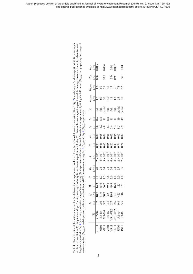
4.3. Experimental dispersion values

The morphological and hydraulic characteristics of the uniform reaches for the different tracer exper-iments are given in Table 4 as well as the dispersion coefficients obtained with the tracing and ADCPmethods. For three of the homogeneous reaches, especially the prismatic Gentille canal (GE11), the dis-persion coefficients obtained from the tracer experiments by fitting the 1-D model (DL,exp) or by applyingthe change of moment method (DL,mmt) are in very close agreement, within a few %. The results of thechange of moment method agree by no more than a factor 2 for all experiments except in the Canal Sudchannel (CS11) where DL,mmt is roughly 5 times greater than DL,exp. This can be explained because simu-lated velocities and depth are actually less uniform throughout that reach than in the others. Subsequently,the model calibration may be poorer in that CS11 reach. DL,mmt can be either lower or greater than DL,exp,which suggests that the 1-D model is not biased by excessive numerical dispersion. Dispersion values ob-tained using the 1-D model, DL,exp, will be kept as the reference values precisely because they are consistentwith the computational assumptions of the model to be calibrated.

The experimental results presented in this work are comparable to the data from literature (see Fig. 1,our data). The aspect ratio, W/H, of the homogeneous reaches ranges from 5 to 50 and the velocity ratio,U/U∗, is spread from 5 to 15, which are situations commonly encountered on the Rhone River and similarmedium-sized rivers. The DL/(HU∗) values obtained from the tracing method vary between 10 and 1000.

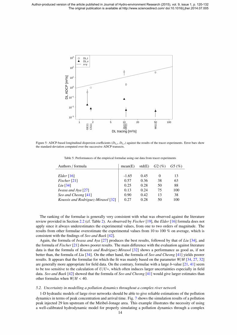
Fig. 5 presents the dimensionless dispersion values obtained with the ADCP method versus the referencevalues obtained from tracing results. As expected, DL,t is always higher than DL,v, and the discrepancybetween the two values spreads from one to four orders of magnitude. This confirms that in most of ourfield cases, the longitudinal dispersion is mainly driven by the transverse velocity gradient, rather than bythe vertical velocity gradient.

For all experiments with available ADCP data, DL,t is in the same order of magnitude as the valueobtained from the tracing method, which suggests that the ADCP method may be an acceptable surrogateto the costly tracing method. Except for the JN11 experiment, DL,t is always lower than DL,exp. Someexplanations can be proposed to such underestimating trend. First, the ADCP method relies on velocityrecorded throughout the whole cross-section. In the GE11 case, the transversal velocities measured bythe ADCP at G4 present a very flat profile and unmeasured areas near edges represent almost 15% of thecross-section. Then, the transversal velocity gradient may not be well captured in such a situation, leadingto an underestimation of the DL,t value. Moreover, the spatial resolution of the ADCP grid and the spatialaveraging by the software may also lead to underrating of the transversal gradient. Both types of issuesmight be mitigated by fitting a continuous function to the transverse profile of the longitudinal velocity, asSeo and Baek [42] did using the beta probability distribution function.

We also highlighted in Section 3.3 that partial mixing of the tracer should be reminded in some reaches,which could have an effect on the DL value from tracer experiment. Besides, the more important differ-ences between DL,t and tracer experiment results in CS11 and, to a lesser extent, in VR11 certainly arisebecause ADCP measurements were conducted in cross-sections that were not fully representative of thereach-averaged hydraulic conditions. Nevertheless, for the cases presented in Fig. 5, the ADCP methodconsidering the transverse velocity gradient as the main driver of the longitudinal dispersion producesdispersion estimates, DL,t, that are in good agreement with the values obtained from tracer experiment.

5. Calibrating dispersion in 1-D hydraulic models

5.1. Performance of dispersion predictors

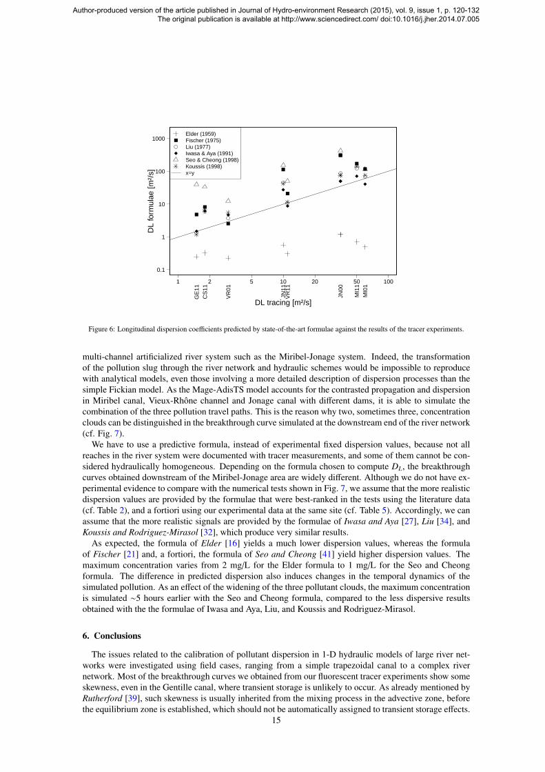
For each tracer experiment, the six formulae from the literature presented in Table 1 were applied tocompute the longitudinal dispersion coefficient, DL. The results are presented in Fig. 6. The four scoresalready presented in Section 2.2 were used to evaluate the performance of the formulae in predicting thedispersion values from our tracer experiments (Table 5).

12


T abl

e4:

Cha

ract

eris

tics

ofth

eun

ifor

mre

ache

sfo

rth

edi

ffer

entt

race

rexp

erim

ents

,as

deriv

edfr

omth

e1-

Dm

odel

:re

ach

boun

dari

es(1

)(cf

.Fig

.2),

reac

hle

ngth

L r,d

isch

arge

Q,w

idth

W,w

ater

dept

hH

,Str

ickl

erco

effici

entK

s,lo

ngitu

dina

lslo

peJ,

sect

ion-

aver

aged

velo

city

U,s

ectio

n-av

erag

edsh

earv

eloc

ityU∗,d

ista

nce

betw

een

inje

ctio

npo

sitio

nan

dth

eho

mog

eneo

usre

ach

star

tLi,

adve

ctiv

ezo

nele

ngth

com

pute

dw

ithE

q.4

(α=

1)L x

,qua

litat

ive

ratin

gof

trac

erm

ixin

g(2

),di

sper

sion

coeffi

cien

tsob

tain

edfr

omth

etr

acer

expe

rim

ents

byfit

ting

the

1-D

mod

el(D

L,ex

p)or

byap

plyi

ngth

ech

ange

ofm

omen

tmet

hod

(DL,

mm

t),a

nddi

sper

sion

coeffi

cien

tsde

rived

from

AD

CP

mea

sure

men

tsus

ing

Eq.

6(D

L,t)

and

Eq.

8(D

L,v)

,res

pect

ivel

y.

L rQ

WH

Ks

JU

U∗

L iL x

(2)

DL,

exp

DL,

mm

tD

L,t

DL,

v

(1)

[km

][m

3 /s]

[m]

[m]

[m1/

3 /s]

[m/m

][m

/s]

[m/s

][k

m]

[km

][m

2 /s]

[m2 /

s][m

2 /s]

[m2 /

s]

GE

11G

2-G

41.

210

.714

.32.

140

2×

10−

50.

300.

020.

80.

6fu

ll1.

51.

60.

320.

015

MI0

1B

3-B

42.

631

.965

.61.

724

4×

10−

40.

460.

0514

.28.

8fu

ll60

59M

I11

M3-

M4

3.2

60.7

66.7

1.5

245×

10−

40.

650.

084.

811

part

ial

5029

32.2

0.00

4V

R01

B5-

B7

3.3

9.5

59.3

3.8

245×

10−

60.

050.

0114

.08.

8fu

ll3.

03.

1V

R11

VR

1-V

R2

2.7

19.4

49.9

2.6

244×

10−

40.

200.

025.

411

full

1117

3.0

0.01

CS1

1C

S1-C

S22.

66.

016

.01.

124

4×

10−

40.

400.

055.

411

full

1.8

9.3

0.93

0.00

7JN

00A

2-A

49.

442

512

55.

035

2×

10−

30.

740.

058.

519

part

ial

3578

JN11

J3-J

65.

514

613

14.

835

7×

10−

50.

240.

022.

949

part

ial

106.

532

0.04

13


1 2 5 10 20 50 100

GE

11C

S11

JN11

VR

11

MI1

1

10−3

10−2

10−1

100

101

102

103

DL tracing [m²/s]

DL

AD

CP

[m²/

s]

DL,tDL,vx=y

Figure 5: ADCP-based longitudinal dispersion coefficients (DL,t , DL,v) against the results of the tracer experiments. Error bars showthe standard-deviation computed over the successive ADCP transects.

Table 5: Performances of the empirical formulae using our data from tracer experiments

Authors / formula mean(E) std(E) G2 (%) G5 (%)

Elder [16] -1.65 0.45 0 13Fischer [21] 0.57 0.36 38 63Liu [34] 0.25 0.28 50 88Iwasa and Aya [27] 0.13 0.24 75 100Seo and Cheong [41] 0.90 0.42 13 38Koussis and Rodriguez-Mirasol [32] 0.27 0.28 50 100

The ranking of the formulae is generally very consistent with what was observed against the literaturereview provided in Section 2.2 (cf. Table 2). As observed by Fischer [19], the Elder [16] formula does notapply since it always underestimates the experimental values, from one to two orders of magnitude. Theresults from other formulae overestimate the experimental values from 10 to 100 % on average, which isconsistent with the findings of Seo and Baek [42].

Again, the formula of Iwasa and Aya [27] produces the best results, followed by that of Liu [34], andthe formula of Fischer [21] shows poorer results. The main difference with the evaluation against literaturedata is that the formula of Koussis and Rodriguez-Mirasol [32] shows a performance as good as, if notbetter than, the formula of Liu [34]. On the other hand, the formula of Seo and Cheong [41] yields poorerresults. It appears that the formulae for which the fit was mainly based on the parameter W/H [34, 27, 32]are generally more appropriate for field data. On the contrary, formulae with a large b-value [21, 41] seemto be too sensitive to the calculation of U/U∗, which often induces larger uncertainties especially in fielddata. Seo and Baek [42] showed that the formula of Seo and Cheong [41] would give larger estimates thanother formulas when W/H < 40.

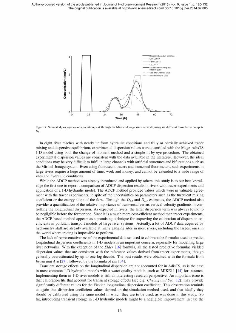
5.2. Uncertainty in modelling a pollution dynamics throughout a complex river network1-D hydraulic models of large river networks should be able to give reliable estimations of the pollution

dynamics in terms of peak concentration and arrival time. Fig. 7 shows the simulation results of a pollutionpeak injected 29 km upstream of the Miribel-Jonage area. This example illustrates the necessity of usinga well-calibrated hydrodynamic model for properly simulating a pollution dynamics through a complex

14


1 2 5 10 20 50 100

GE

11C

S11

VR

01

JN11

VR

11

JN00

MI1

1M

I01

0.1

1

10

100

1000

DL tracing [m²/s]

DL

form

ulae

[m²/

s]

Elder (1959)Fischer (1975)Liu (1977)Iwasa & Aya (1991)Seo & Cheong (1998)Koussis (1998)x=y

Figure 6: Longitudinal dispersion coefficients predicted by state-of-the-art formulae against the results of the tracer experiments.

multi-channel artificialized river system such as the Miribel-Jonage system. Indeed, the transformationof the pollution slug through the river network and hydraulic schemes would be impossible to reproducewith analytical models, even those involving a more detailed description of dispersion processes than thesimple Fickian model. As the Mage-AdisTS model accounts for the contrasted propagation and dispersionin Miribel canal, Vieux-Rhone channel and Jonage canal with different dams, it is able to simulate thecombination of the three pollution travel paths. This is the reason why two, sometimes three, concentrationclouds can be distinguished in the breakthrough curve simulated at the downstream end of the river network(cf. Fig. 7).

We have to use a predictive formula, instead of experimental fixed dispersion values, because not allreaches in the river system were documented with tracer measurements, and some of them cannot be con-sidered hydraulically homogeneous. Depending on the formula chosen to compute DL, the breakthroughcurves obtained downstream of the Miribel-Jonage area are widely different. Although we do not have ex-perimental evidence to compare with the numerical tests shown in Fig. 7, we assume that the more realisticdispersion values are provided by the formulae that were best-ranked in the tests using the literature data(cf. Table 2), and a fortiori using our experimental data at the same site (cf. Table 5). Accordingly, we canassume that the more realistic signals are provided by the formulae of Iwasa and Aya [27], Liu [34], andKoussis and Rodriguez-Mirasol [32], which produce very similar results.

As expected, the formula of Elder [16] yields a much lower dispersion values, whereas the formulaof Fischer [21] and, a fortiori, the formula of Seo and Cheong [41] yield higher dispersion values. Themaximum concentration varies from 2 mg/L for the Elder formula to 1 mg/L for the Seo and Cheongformula. The difference in predicted dispersion also induces changes in the temporal dynamics of thesimulated pollution. As an effect of the widening of the three pollutant clouds, the maximum concentrationis simulated ∼5 hours earlier with the Seo and Cheong formula, compared to the less dispersive resultsobtained with the the formulae of Iwasa and Aya, Liu, and Koussis and Rodriguez-Mirasol.

6. Conclusions

The issues related to the calibration of pollutant dispersion in 1-D hydraulic models of large river net-works were investigated using field cases, ranging from a simple trapezoidal canal to a complex rivernetwork. Most of the breakthrough curves we obtained from our fluorescent tracer experiments show someskewness, even in the Gentille canal, where transient storage is unlikely to occur. As already mentioned byRutherford [39], such skewness is usually inherited from the mixing process in the advective zone, beforethe equilibrium zone is established, which should not be automatically assigned to transient storage effects.

15


02/06/11 00:00 02/06/11 12:00 03/06/11 00:00 03/06/11 12:00 04/06/11 00:00 04/06/11 12:00 05/06/11 00:000

0

0

0

Elder, 1959

Fisher, 1975

Liu, 1977

Koussis and Rodriguez-Mirasol, 1998

Seo and Cheong, 1998

Iwasa and Aya, 1991

Upstream boundary condition

0 12 24 36 48 60 720

1

2

Time (h)

3

Co

nc

entr

atio

n (

mg

/L)

Figure 7: Simulated propagation of a pollution peak through the Miribel-Jonage river network, using six different formulae to computeDL.

In eight river reaches with nearly uniform hydraulic conditions and fully or partially achieved tracermixing and dispersive equilibrium, experimental dispersion values were quantified with the Mage-AdisTS1-D model using both the change of moment method and a simple fit-by-eye procedure. The obtainedexperimental dispersion values are consistent with the data available in the literature. However, the idealconditions may be very difficult to fulfil in large channels with artificial structures and bifurcations such asthe Miribel-Jonage system. Even using fluorescent tracers and immersed fluorimeters, such experiments inlarge rivers require a huge amount of time, work and money, and cannot be extended to a wide range ofsites and hydraulic conditions.

While the ADCP method was already introduced and applied by others, this study is to our best knowl-edge the first one to report a comparison of ADCP dispersion results in rivers with tracer experiments andapplication of a 1-D hydraulic model. The ADCP method provided values which were in valuable agree-ment with the tracer experiments, in spite of the uncertainties on parameters such as the turbulent mixingcoefficient or the energy slope of the flow. Through the DL,t and DL,v estimates, the ADCP method alsoprovides a quantification of the relative importance of transversal versus vertical velocity gradients in con-trolling the longitudinal dispersion. As expected in rivers, the latter dispersion term was always found tobe negligible before the former one. Since it is a much more cost-efficient method than tracer experiments,the ADCP-based method appears as a promising technique for improving the calibration of dispersion co-efficients in pollutant transport models of large river systems. Actually, a lot of ADCP data acquired byhydrometry staff are already available at many gauging sites in most rivers, including the largest ones inthe world where tracing is impossible to perform.

The lack of representativeness of the experimental data set used to calibrate the formulae used to predictlongitudinal dispersion coefficients in 1-D models is an important concern, especially for modelling largeriver networks. With the exception of the Elder [16] formula, all the tested predictive formulae yieldeddispersion values that are consistent with the reference values derived from tracer experiments, thoughgenerally overestimated by up to one log decade. The best results were obtained with the formula fromIwasa and Aya [27], followed by the formula of Liu [34].

Transient storage effects on the longitudinal dispersion are not accounted for in AdisTS, as is the casein most common 1-D hydraulic models with a water quality module, such as MIKE11 [14] for instance.Implementing them in 1-D river models is still an interesting research perspective. An important issue isthat calibration fits that account for transient storage effects (see e.g. Cheong and Seo [12]) may providesignificantly different values for the Fickian longitudinal dispersion coefficient. This observation remindsus again that dispersion coefficient values depend on the simulation method used, and that ideally theyshould be calibrated using the same model in which they are to be used, as was done in this study. Sofar, introducing transient storage in 1-D hydraulic models might be a negligible improvement, in case the

16


mainstream longitudinal dispersion coefficient is not parameterized accurately based on an appropriatepredictive formula.

7. Acknowledgements

This work has been conducted in the framework of the Rhone Sediment Observatory project and waspartly funded by the Plan Rhone. The PhD scholarship of Marina Launay was granted by the RegionRhone-Alpes (convention number: 12-013144-01 for the PhD third year).

References

[1] Andries, E., Le Coz, J., Camenen, B., Faure, J.-B., and Launay, M. (2011). Impact of dam flushes on bed clogging in a secondarychannel of the Rhone river. Proceedings of RCEM (River, Coastal and Estuarine Morphodynamics), Beijing, China, 10 p.

[2] Andre, H., Audinet, M., Mazeran, G., and Richer, C. (1976). Hydrometrie pratique des cours d’eau. [Practical hydrometry inrivers]. Direction des etudes et des recherches d’Electricite de France (EDF), 88 p. (in French)

[3] Andre, J. and Molinari, J. (1976). Mises au point sur les differents facteurs physico-chimiques influant sur la mesure de traceursfluorescents et leurs consequences pratiques en hydrologie. [Clarifications on the various physico-chemical factors affecting thedegree of fluorescent tracers and their practical implications in hydrology]. Journal of Hydrology, 30:257–285. (in French)

[4] Biron, P., Ramamurthy, A., and Han, S. (2004). Three-dimensional numerical modeling of mixing at river confluences. Journalof Hydraulic Engineering, 130(3):243–253.

[5] Bencala, K.E., and Walters, R.A. (1983). Simulation of Solute Transport in a Mountain Pool-and-Riffle Stream: A TransientStorage Model. Water Resources Research, 19(3):718–724.

[6] Bottacin-Busolin, A., Marion, Musner, T., Tregnaghi, M., and Zaramella M. (2011). Evidence of distinct contaminant transportpatterns in rivers using tracer tests and a multiple domain retention model. Advances in Water Resources, 34:737–746.

[7] Boiten, W. (2000). Hydrometry. Francis and Taylor publishers, 257 p.[8] Caplow, T., Schlosser, P., and Ho, D. (2004). Tracer study of mixing and transport in the upper Hudson River with multiple dams.

Journal of Hydraulic Engineering, 130(12):1498–1506.[9] Carr, M. and Rehmann, C. (2007). Measuring the dispersion coefficient with acoustic Doppler current profilers. Journal of

Hydraulic Engineering, 133(8):977–982.[10] Chatwin, P. (1971). On the interpretation of some longitudinal dispersion experiments. Journal of Fluid Mechanics, 48(4):689–

702.[11] Chatwin, P. (1980). Presentation of longitudinal dispersion data. Journal of Hydraulic Divisions, 106(1):71–83.[12] Cheong, T., and Seo, I. (2003). Parameter estimation of the transient storage model by a routing method for river mixing

processes. Water Resources Research, 39(4):1–11.[13] Davis, S., Thompson, G., Bentley, H., and Stiles, G. (1980). Ground-water tracers - A short review. Ground Water, 18(1):14–23.[14] DHI (2009). MIKE11 - A Modelling System for Rivers and Channels. Reference Manual, 524 p.[15] Duarte, A. A. and Boaventura, R. A. (2008). Dispersion modelling in rivers for water sources protection, based on tracer

experiments. Case studies. In Mastorakis, N.E., Poulos, M., Mladenov, V., Bojkovic, Z., Simian, D. and Kartalopoulos, S.,editor, Proc. 2nd Int. Conf. on Waste Management, Water Pollution, Air Pollution, Indoor Climate, Energy and EnvironmentalEngineering Series, pages 205–210, Corfu, Greece.

[16] Elder, J. (1959). The dispersion of marked fluid in turbulent shear flow. Journal of Fluid Mechanics, 5(4):544?560.[17] Fassnacht, S. (1997). A multi-channel suspended sediment transport model for the Mackenzie Delta, Northwest Territories.

Journal of Hydrology, 197:128-145.[18] Field, M., Wilhem, R., Equilan, J., and Aley, T. (1995). An assessment of the potential adverse properties of fluorescent tracer

dyes used for groundwater tracing. Environmental Monitoring and Assessment, 38:7596.[19] Fischer, H. (1966). Longitudinal dispersion in laboratory and natural streams. Report KH-R-12, Keck Laboratory of hydraulics

and water resources, California Institute of Technology, Pasadena, California, USA. 265 p.[20] Fischer, H. (1968). Dispersion predictions in natural streams. J. Sanit. Eng. Div., ASCE, 94(SA5):927–943.[21] Fischer, H. (1975). Discussion of simple method for predicting dispersion in stream by R. S. McQuivey and T. N. Keefer.

Journal of Environmental Engineering Division, 101(3):453?455.[22] Fischer, H., List, E., Koh, R., Imberger, J., and Brooks, N. (1979). Mixing in Inland and Coastal Waters. Academic Press, New

York. 497 p.[23] Flury, M. and Wai, N. (2003). Dyes as tracers for vadose zone hydrology. Reviews of Geophysics, 41:1002.[24] Gooseff, M.N., Hall JR., R.O., and Tank, J.L. (2005). Relating transient storage to channel complexity in streams of varying

land use in Jackson Hole, Wyoming. Water Resources Research, 43(W01417):1–10.[25] Ho, D., Schlosser, P., and Caplow, T. (2002). Determination of longitudinal dispersion coefficient and net advection in the

tidal Hudson River with a large-scale, high resolution SF6 tracer release experiment. Environmental Science & Technology,36(15):3234–3241.

[26] Hubbard, E., Kilpatrick, F., Martens, L., and Wilson, J. (1982). Measurement of time of travel and dispersion in streams by dyetracing. Techniques of Water- Resources Investigations, vol. 3, 44 p.

[27] Iwasa, Y. and Aya, S. (1991). Predicting longitudinal dispersion coefficient in open channel flows. In Int. Symp. on Environ-mental Hydraulics, pages 505–510, Hong-Kong, China.

[28] Jobson, H. (1997). Predicting travel time and dispersion in rivers and streams. Journal of Hydraulic Engineering-ASCE,123(11):971–978.

17


[29] Jobson, H. (2001). Predicting river travel time from hydraulic characteristics. Journal of Hydraulic Engineering-ASCE,127(11):911–918.

[30] Kilic, S.G., and Aral, M.M. (2009). A fugacity based continuous and dynamic fate and transport model for river networks andits application to Altamaha River. Science of the total environment,407(12):3855–3866.

[31] Kim, D. (2012). Assessment of longitudinal dispersion coefficients using Acoustic Doppler Current Profilers in large river.Journal of Hydro-Environment Research, 6(1):29–39.

[32] Koussis, A. and Rodriguez-Mirasol, J. (1998). Hydraulic estimation of dispersion coefficient for streams. Journal of HydraulicEngineering-ASCE, 124(3):317–320.

[33] Leibundgut, C., Maloszewski, P., and Kulls, C. (2009). Tracers in Hydrology. Wiley-Blackwell.[34] Liu, H. (1977). Predicting dispersion coefficient of streams. Journal of the Environmental Engineering Division, 103(1):59–69.[35] Magazine, M., Pathak, S. and Pande, P. (1988). Effect of bed and side roughness on dispersion coefficient in natural streams.

Journal of Hydraulic Engineering, 114(7):766–782.[36] Marion, A., Zaramella, M., and Bottacin-Busolin, A. (2008). Solute transport in rivers with multiple storage zones: The STIR

model. Water Resources Research, 44(10), W10406.[37] Nordin Jr., C.F.N. and Troutman, B. M. (1980). Longitudinal dispersion in rivers: The persistence of skewness in observed data.

Water Resources Research, 16(1):123–128.[38] Rowinski, P., Guymer, I., and Kwiatkowski, K. (2008). Response to the slug injection of a tracer-a large-scale experiment in a

natural river. Hydrological Sciences Journal, 53(6):1300–1309.[39] Rutherford, J. (1994). River Mixing. Wiley. 362 p.[40] Scheidegger, A. (1961). General theory of dispersion in porous media. Journal of Geophysical Research, 66:3273–3278.[41] Seo, I. and Cheong, T. (1998). Predicting longitudinal dispersion coefficient in natural streams. Journal of Hydraulic

Engineering-ASCE, 124(1):25–32.[42] Seo, I. and Baek, K. (2004). Estimation of the longitudinal dispersion coefficient using the velocity profile in natural streams.

Journal of Hydraulic Engineering-ASCE, 130:227–236.[43] Shen, C., Niu, J., Anderson, E., and Phanikumar, M. (2010). Estimating longitudinal dispersion in rivers using Acoustic Doppler

Current Profilers. Advances in Water Resources, 33(6):615–623.[44] Smart, P. (1984). A review of the toxicity of twelve fluorescent dyes used for water tracing. The National Speleological Society

Bulletin, 46:21.[45] Smart, P. and Laidlaw, I. (1977). An evaluation of some fluorescent dyes for water tracing. Water Resources Research, 13

(1):15–33.[46] Souhar, O., and Faure, J.-B. (2009). Approach for uncertainty propagation and design in Saint Venant equations via automatic

sensitive derivatives applied to Saar river. Canadian Journal of Civil Engineering 36 (7), 1144–1154.[47] Steinheimer, T. and Johnson, S. (1986). Investigation of the possible formation of diethylnitrosamine resulting from the use of

rhodamine WT dye as a tracer in river waters. USGS WSP 2290, 2290:37.[48] Szeftel, P., Moore, R.D., and Weiler, M. (2011). Influence of distributed flow losses and gains on the estimation of transient

storage parameters from stream tracer experiments. Journal of Hydrology, 396, 277–291.[49] Taylor, G. (1954). The dispersion of matter in turbulent flow through a pipe. In Royal society, volume A, pages 446–468.[50] Wilson, J., Cobb, E., and Kilpatrick, F. (1986). Fluorometric procedures for dye tracing. Techniques of Water-Resources

Investigations, vol. 3, 31 p.[51] Worman, A. and Wachniew, P. (2007). Reach scale and evaluation methods as limitations for transient storage properties in

streams and rivers. Water Resources Research, 43, W10405.

18


Documents

Calibrating pollutant dispersion in 1-D hydraulic models