Embed Size (px)
Citation preview
Project Number: MQP KZN 981
COMPUTATIONAL MODELING OF FIRE SPRINKLER SPRAY
CHARACTERISTICS USING THE FIRE DYNAMICS SIMULATOR
A Major Qualifying Project Report Submitted to the Faculty of
WORCESTER POLYTECHNIC INSTITUTE
in partial fulfillment of the requirements for the
Degree of Bachelor of Science
By:
______________________ Matthew J. Bourque
______________________ Thomas A. Svirsky
Date: 25 April 2013
Approved By:
_____________________________________ Professor Kathy Notarianni, Primary Advisor
Keywords 1. Sprinkler 2. FDS 3. Computational Fluid Dynamics

2
Acknowledgements
We would like to thank the following people for their help and guidance they provided
throughout the project. This project would not have been possible with the assistance of the
following people:
Dr. Kathy Notarianni – Primary Advisor, WPI
Raymond Ranellone – Graduate Research Assistant, WPI
Jeffery Rosen – Graduate Research Assistant, WPI
Michael Szkutak – Graduate Research Assistant, WPI
Dr. Kevin McGrattan - NIST
Dr. Pravinray Gandhi – UL Director of Corporate Research
David Dubiel – UL Research Engineer
Christian Martinez – UL Lab Technician
Melissa Avila – Engineering Manager, Tyco
Katerina Stavrianidis – Project Engineer, Tyco
3
Table of Contents Acknowledgements ...................................................................................................................................... 2
Table of Figures ........................................................................................................................................... 5
List of Tables ............................................................................................................................................... 6
Abstract ........................................................................................................................................................ 7
1.0 Introduction ............................................................................................................................................ 8
2.0 Background ............................................................................................................................................ 9
3.0 Research Plan ....................................................................................................................................... 12
4.0 Spray Characteristics ........................................................................................................................... 13
4.1 Shape of Spray (Spray Angle) ......................................................................................................... 13
4.2 Velocity ............................................................................................................................................ 14
4.3 Droplet Size ..................................................................................................................................... 19
4.4 Water Flux ....................................................................................................................................... 20
4.5 Spray Offset ..................................................................................................................................... 22
5.0 Measurement Methods ......................................................................................................................... 23
5.1 Particle Image Velocimetry ............................................................................................................. 23
5.2 Phase Doppler Anemometry ............................................................................................................ 26
5.3 Direct Image Particle Analysis (DIPA) ............................................................................................ 26
6.0 The Fire Dynamics Simulator .............................................................................................................. 27
6.1 Physics and Underlying Equations in FDS 6 ................................................................................... 27
6.1.1 Number of Particles .................................................................................................................. 28
6.1.2 Particle Size Distribution .......................................................................................................... 29
6.2 Limitations ....................................................................................................................................... 30
6.3 List of Relevant Inputs and Defaults ................................................................................................ 31
7.0 Characterization of Upright Extended Coverage k-25.2 Fire Sprinkler ............................................... 32
7.1 Manufacturer’s Data ........................................................................................................................ 32
7.2 Underwriter’s Laboratories Experiments ......................................................................................... 32
7.2.1 Sprinkler Setup ......................................................................................................................... 32
7.2.2 PIV Setup .................................................................................................................................. 32
7.2.3 DIPA Setup ............................................................................................................................... 33
7.3 Measured Model Inputs ................................................................................................................... 34
7.3.1 Spray Angle .............................................................................................................................. 34
4
7.3.2 Droplet Size .............................................................................................................................. 35
7.3.3 Spray Offset .............................................................................................................................. 36
7.3.4 Initial Velocity .......................................................................................................................... 38
8.0 Characterization of Pendant k5.6 Sprinkler ......................................................................................... 39
8.1 Measured Model Inputs ................................................................................................................... 39
8.1.1 Spray Angle .............................................................................................................................. 39
8.1.2 Droplet Size .............................................................................................................................. 40
8.1.3 Spray Offset .............................................................................................................................. 41
8.1.4 Initial Velocity .......................................................................................................................... 41
9.0 Prediction of Actual Delivered Density (ADD) with FDS and Comparison to Measured ADD for K25.2 Sprinkler .......................................................................................................................................... 41
9.1 Tyco Experiments ............................................................................................................................ 41
9.2 Tyco Bucket Test Collection Data Collection .................................................................................. 42
9.3 Sources of Error ............................................................................................................................... 44
9.3.1 Ramp-up time ........................................................................................................................... 44
9.3.2 Measurement techniques ........................................................................................................... 45
9.3.3 Fluctuating flow rate ................................................................................................................. 45
9.3.4 Ceiling effects ........................................................................................................................... 46
9.3.5 Total Uncertainty: ..................................................................................................................... 46
10.0 Prediction of Actual Delivered Density (ADD) with FDS and Comparison to Measured ADD for k5.6 Sprinkler ............................................................................................................................................ 46
10.1 Tyco Experiments .......................................................................................................................... 46
10.2 Tyco Bucket Test Collection Data Collection ................................................................................ 47
10.3 Sources of Error ............................................................................................................................. 48
10.3.1 Ramp-up time ......................................................................................................................... 48
10.3.2 Measurement techniques ......................................................................................................... 49
10.3.3 Fluctuating flow rate ............................................................................................................... 49
10.3.4 Ceiling effects ......................................................................................................................... 49
10.3.5 Total Uncertainty: ................................................................................................................... 50
11.0 FDS Testing ....................................................................................................................................... 50
12.0 Results of Sensitivity Analysis .......................................................................................................... 57
12.1 Base Case and Results ................................................................................................................... 58
5
12.2 Offset: ............................................................................................................................................ 59
12.3 Spray Angle: .................................................................................................................................. 59
12.4 Droplet Size: .................................................................................................................................. 60
12.5 Velocity: ........................................................................................................................................ 61
12.6 Particles per second: ...................................................................................................................... 62
12.7 Default Values: .............................................................................................................................. 62
13.0 Conclusions and Recommendations .................................................................................................. 63
References ................................................................................................................................................. 65
Appendix A: Offset .................................................................................................................................... 67
Appendix B: Spray Angle from PIV .......................................................................................................... 73
Appendix C: Spray Angle from Camera .................................................................................................... 80
Appendix D: Spray Velocities ................................................................................................................... 85
Appendix E: Spray Velocity Contour Maps .............................................................................................. 88
Appendix F: Pictures from Tyco ................................................................................................................ 91
Table of Figures 1: Contour map of bucket test water flux density distribution in L/m2 [3] ................................................. 11 Figure 2: Contour map of FDS water flux density distribution in L/m2 [3] ............................................... 11 Figure 3: Sprinkler Spray Shapes [1] ......................................................................................................... 13 Figure 4: Inner Spray Angle ...................................................................................................................... 14 Figure 5: Initial Velocities vs. Terminal Velocity [1] ................................................................................ 16 Figure 6: Initial Horizontal Velocity [1] .................................................................................................... 17 Figure 7: Horizontal Distances [1] ............................................................................................................. 18 Figure 8: Droplet Velocity vs. Water Pressure [1] ..................................................................................... 19 Figure 9: Ligament Breakup (Marshall) .................................................................................................... 23 Figure 10- PIV Setup ................................................................................................................................. 25 Figure 11- Vector Field [10] ...................................................................................................................... 25 Figure 12: Phase Doppler Anemometer Diagram [14] .............................................................................. 26 Figure 13: DIPA Setup [4] ......................................................................................................................... 27 Figure 14: Outside Spray Angle [3] ........................................................................................................... 34 Figure 15 - Dave Sheppard's Droplet Size Analysis .................................................................................. 36 Figure 16: Spray Offset at 15 Degrees ....................................................................................................... 38 Figure 17: Velocity Radial Scatter Plot ..................................................................................................... 39 Figure 18: Dave Sheppard's Droplet Size Analysis ................................................................................... 40 Figure 19: Tyco Bucket Test Setup ........................................................................................................... 42
6
Figure 20: Tyco Bucket Test Setup ........................................................................................................... 47 Figure 21 - 0500Deg .................................................................................................................................. 67 Figure 22 - 1500Deg .................................................................................................................................. 68 Figure 23 - 3000Deg .................................................................................................................................. 69 Figure 24 - 4500Deg .................................................................................................................................. 70 Figure 25 - 6000Deg .................................................................................................................................. 71 Figure 26 - 7500Deg .................................................................................................................................. 72 Figure 27:0500Deg .................................................................................................................................... 73 Figure 28 - 1500Deg .................................................................................................................................. 74 Figure 29 - 3000Deg .................................................................................................................................. 75 Figure 30 - 4500Deg .................................................................................................................................. 76 Figure 31 - 6000Deg .................................................................................................................................. 77 Figure 32 - 7500Deg .................................................................................................................................. 78 Figure 33 - 8500Deg .................................................................................................................................. 79 Figure 34 - 0500 Velocity Contour Plot ..................................................................................................... 88 Figure 35 - 1500 Velocity Contour Plot ..................................................................................................... 88 Figure 36 - 3000 Velocity Contour Plot ..................................................................................................... 89 Figure 37 - 4500 Velocity Contour Plot ..................................................................................................... 89 Figure 38 - 6000 Velocity Contour Plot ..................................................................................................... 90 Figure 39 - 7500 Velocity Contour Plot ..................................................................................................... 90 Figure 40: Calibrated Dipstick ................................................................................................................... 91 Figure 41: Ruler Measurement .................................................................................................................. 91 Figure 42: Droplets on Ceiling .................................................................................................................. 92 Figure 43: Flow Meter Display .................................................................................................................. 93
List of Tables Table 1: Droplet Diameter vs. Reynolds Number vs. Terminal Velocity [1] ............................................ 15 Table 2: Vertical Distances [1] .................................................................................................................. 16 Table 3: FDS Inputs ................................................................................................................................... 31 Table 4: k-25.2 Manufacturer's Data ......................................................................................................... 32 Table 5: k-5.6 Manufacturer's Data ........................................................................................................... 39 Table 6: Tyco Bucket Test Results ............................................................................................................ 44 Table 7: Tyco Bucket Test Results ............................................................................................................ 48 Table 8: FDS inputs for K25.2 sprinkler .................................................................................................... 50 Table 9: FDS results for K25.2 Sprinkler .................................................................................................. 51 Table 10: Percent difference of bucket test data and FDS results .............................................................. 52 Table 11: FDS inputs for K5.6 sprinkler .................................................................................................... 53 Table 12: FDS results for K5.6 sprinkler ................................................................................................... 53 Table 13: Percent difference between bucket test and FDS test for K5.6 sprinkler ................................... 54 Table 14: FDS results for K5.6 sprinkler simulation with 4 sprinkler setup .............................................. 55
7
Table 15: Percent difference between bucket test results and FDS simulation for 4 sprinkler setup ......... 56 Table 16: Base Case ................................................................................................................................... 58 Table 17: Spray Offset ............................................................................................................................... 59 Table 18: Spray Angle ............................................................................................................................... 60 Table 19: Droplet Size ............................................................................................................................... 61 Table 20: Spray Velocity ........................................................................................................................... 61 Table 21: Particles per Second ................................................................................................................... 62 Table 22: Default Values ........................................................................................................................... 63
Abstract
Large-scale testing is necessary to verify a specific sprinkler’s performance in order for
the sprinkler to become listed and approved. An example of a sprinkler certification test is an
actual density delivered (ADD) test. An ADD test requires the use of a large lab space, lab
assistants, and expensive lab equipment. By using computational fluid dynamics, the cost and
time of this certification process could be reduced. The goal of this project is to determine how
accurately the Fire Dynamics Simulator (FDS) 6 can predict the distribution of water of an
automatic fire sprinkler by inputting the manufacturer’s specifications and measured
characteristics: spray angle, spray offset, initial velocity and droplet size. A sensitivity analysis
was completed to document the relative importance of each model input in the FDS 6 simulation.
These model inputs were measured through use of Particle Image Velocimetry, digital images of
spray, and historical data. The FDS 6 output of water flux distribution was compared to
experimental results of a bucket test. Future testing should include more accurate and simpler
methods for obtaining the model inputs as well as a larger sample size of different fire sprinklers.
8
1.0 Introduction
The purpose of this project is to determine how accurately the Fire Dynamics Simulator
(FDS) 6 can predict the distribution of water of an automatic fire sprinkler by inputting the
manufacturer’s specifications and measured characteristics: spray angle, spray offset, initial
velocity and droplet size. By using computational fluid dynamics the process of measuring water
flux distributions can be more efficient. Testing in a laboratory can become very expensive and
an alternative way to test these sprinklers is needed. An upright extended coverage k-25.2
sprinkler and a k5.6 pendant standard coverage sprinkler were selected for observation.
Experimental data for the model inputs were found at Underwriter’s Laboratories in Northbrook,
Illinois as well as at Tyco in Cranston, Rhode Island. After collecting the data needed to input
into FDS and gathering the manufacturer’s data on the specific sprinkler, FDS testing was
conducted. The water flux distributions produced by FDS were compared to experimental bucket
tests to measure the accuracy of FDS. A flow rate was calculated over each area underneath the
sprinkler using 16 buckets in the experiment and using 16 measuring devices in FDS.
Furthermore a sensitivity analysis was completed to gain an understanding of the relative
importance to each model input. Each major input was raised and lowered from the true value to
observe the fluctuation of water flux distribution. Further research in this area is needed to
validate the FDS characterization of a fire sprinkler by including various types and orientations
of sprinklers.
9
2.0 Background
Sprinkler testing is an expensive and time consuming process. By using Fire Dynamics
Simulator (FDS), the cost and time of this process for large scale testing can be reduced.
However, for FDS to accurately model sprays, the spray characteristics needed to be studied.
Dave Sheppard completed his PhD dissertation at Northwestern, with a goal to “measure the
sprinkler spray characteristics required as input for computational sprinkler spray models [1].”
This project was funded by National Institute of Standard and Technology (NIST) with the
intentions of modifying and updating their sprinkler setup [1-2]. Therefore Sheppard wanted to
understand which inputs were required and important to replicate a sprinkler test in FDS.
Sheppard studied nine pendant and six upright sprinklers with varying k-factors and orifice sizes.
To conduct testing Particle Image Velocimetry (PIV) and Phase Doppler Anemometer (PDA)
were used to study initial spray characteristics.
Some of the main findings that Sheppard found were:
• The major characteristics for characterizing a spray were droplet size, droplet
velocity, and water flux
• Radial droplet velocity at a distance 0.2m from the sprinkler orifice is 53% of the
water velocity through the orifice with a 0.08 standard deviation.
• Radial velocity is dependent on the elevation angle meaning measurements of
spray angles are important.
• The median droplet diameter increases with elevation angle and decreases with
increasing water pressure.
• Water flux is dependent on elevation angle an azithumal angle
10
• It is possible to predict water flux distributions from a PIV
These findings help prove that knowing the sprinkler offset distance is important to
modeling. Also, elevation angle can affect droplet velocities, water flux, and droplet diameters.
Lastly, Sheppard concluded if the initial droplet velocity, droplet direction, number of droplets,
and droplet size were known, a water flux distribution could be predicted. Kevin McGrattan at
NIST used Sheppard’s findings to write a complex detailed file format for inputting sprinkler
data such as spray pattern, droplet size, and droplet velocity for FDS 3. This file format is similar
to the TABL function in FDS 6, but more complicated. However to create this data file, data
from PIV and PDA would need to be used. Before validating this new sprinkler algorithm, it was
removed due to the high cost and inconvenience to running tests in order to gather the inputs.
The sprinkler model was brought back to what it was in FDS 2 where it was simpler and easier to
input values.
A recent study was conducted using the latest version of the computational fluid model,
FDS 6 Beta [3]. Recently a Victoria University group in Australia has tried to characterize a
water-mist spray using FDS 6[3]. To gather their basic sprinkler inputs, manufacturer data sheets
were used. The group then measured outside spray angle by observing a picture and assumed the
inside spray angle was zero. Then the DV50 number was found through “a function of nozzle
orifice diameter, operating pressure, and geometry.” They also assigned the location of the initial
velocity at the orifice in FDS instead of the offset. The group did not specify what was used as an
offset or if it was even measured. However, since it is a nozzle making mist, the offset will not
be very large, which also limits the error of setting the initial velocity at the orifice. Therefore
these errors are minor. The output was a water flux density distribution which was compared to
the one measured with a bucket test. The result was decently successful.
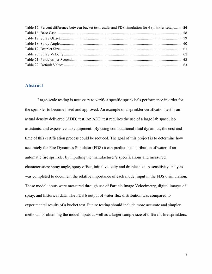
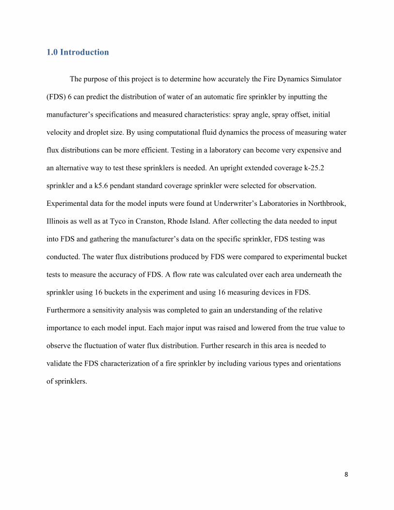
11
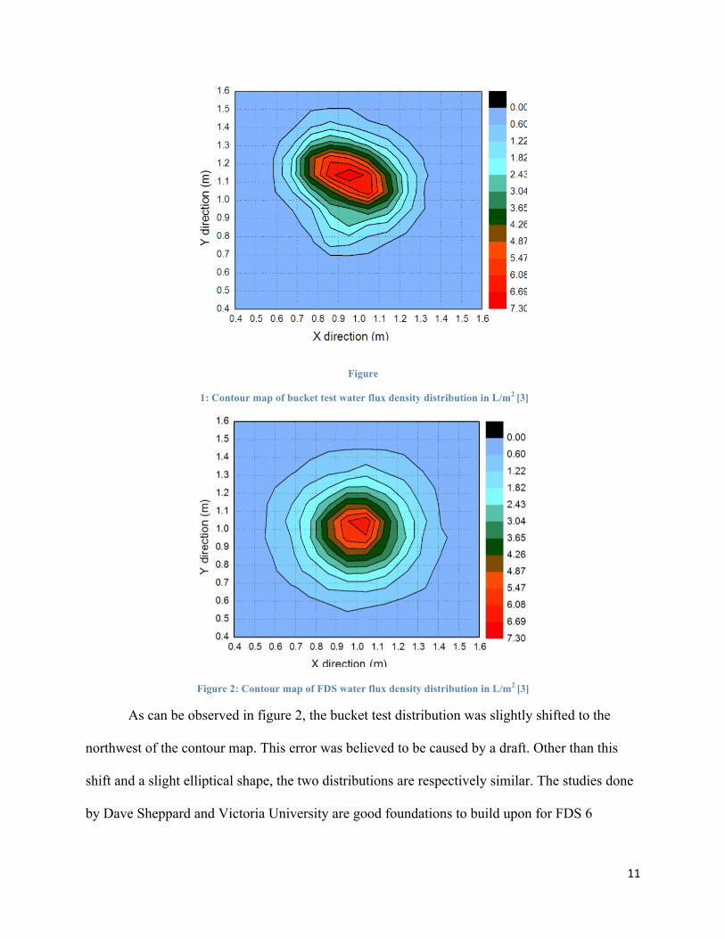
Figure
1: Contour map of bucket test water flux density distribution in L/m2 [3]
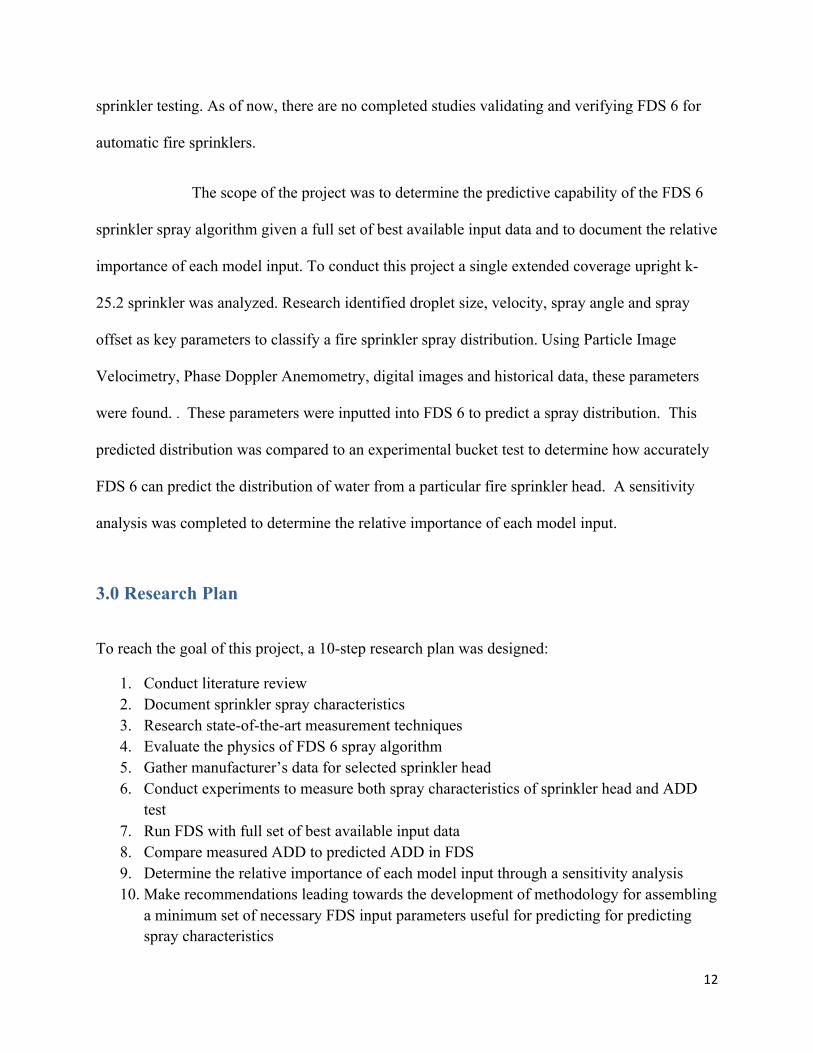
Figure 2: Contour map of FDS water flux density distribution in L/m2 [3]
As can be observed in figure 2, the bucket test distribution was slightly shifted to the
northwest of the contour map. This error was believed to be caused by a draft. Other than this
shift and a slight elliptical shape, the two distributions are respectively similar. The studies done
by Dave Sheppard and Victoria University are good foundations to build upon for FDS 6
12
sprinkler testing. As of now, there are no completed studies validating and verifying FDS 6 for
automatic fire sprinklers.
The scope of the project was to determine the predictive capability of the FDS 6
sprinkler spray algorithm given a full set of best available input data and to document the relative
importance of each model input. To conduct this project a single extended coverage upright k-
25.2 sprinkler was analyzed. Research identified droplet size, velocity, spray angle and spray
offset as key parameters to classify a fire sprinkler spray distribution. Using Particle Image
Velocimetry, Phase Doppler Anemometry, digital images and historical data, these parameters
were found. . These parameters were inputted into FDS 6 to predict a spray distribution. This
predicted distribution was compared to an experimental bucket test to determine how accurately
FDS 6 can predict the distribution of water from a particular fire sprinkler head. A sensitivity
analysis was completed to determine the relative importance of each model input.
3.0 Research Plan
To reach the goal of this project, a 10-step research plan was designed:
1. Conduct literature review 2. Document sprinkler spray characteristics 3. Research state-of-the-art measurement techniques 4. Evaluate the physics of FDS 6 spray algorithm 5. Gather manufacturer’s data for selected sprinkler head 6. Conduct experiments to measure both spray characteristics of sprinkler head and ADD
test 7. Run FDS with full set of best available input data 8. Compare measured ADD to predicted ADD in FDS 9. Determine the relative importance of each model input through a sensitivity analysis 10. Make recommendations leading towards the development of methodology for assembling
a minimum set of necessary FDS input parameters useful for predicting for predicting spray characteristics
13
4.0 Spray Characteristics
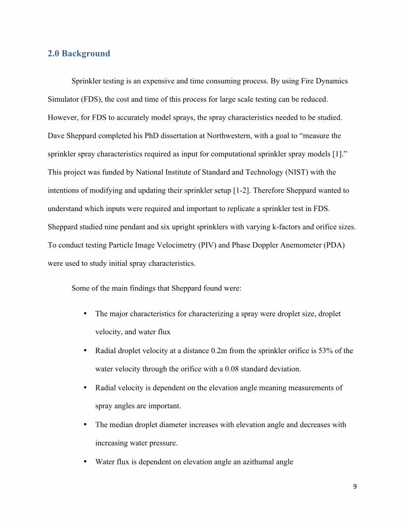
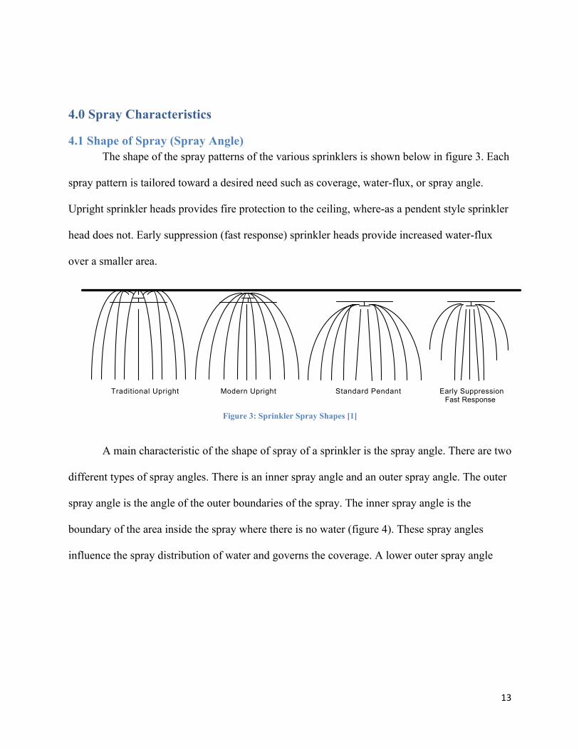
4.1 Shape of Spray (Spray Angle) The shape of the spray patterns of the various sprinklers is shown below in figure 3. Each
spray pattern is tailored toward a desired need such as coverage, water-flux, or spray angle.
Upright sprinkler heads provides fire protection to the ceiling, where-as a pendent style sprinkler
head does not. Early suppression (fast response) sprinkler heads provide increased water-flux
over a smaller area.
Figure 3: Sprinkler Spray Shapes [1]
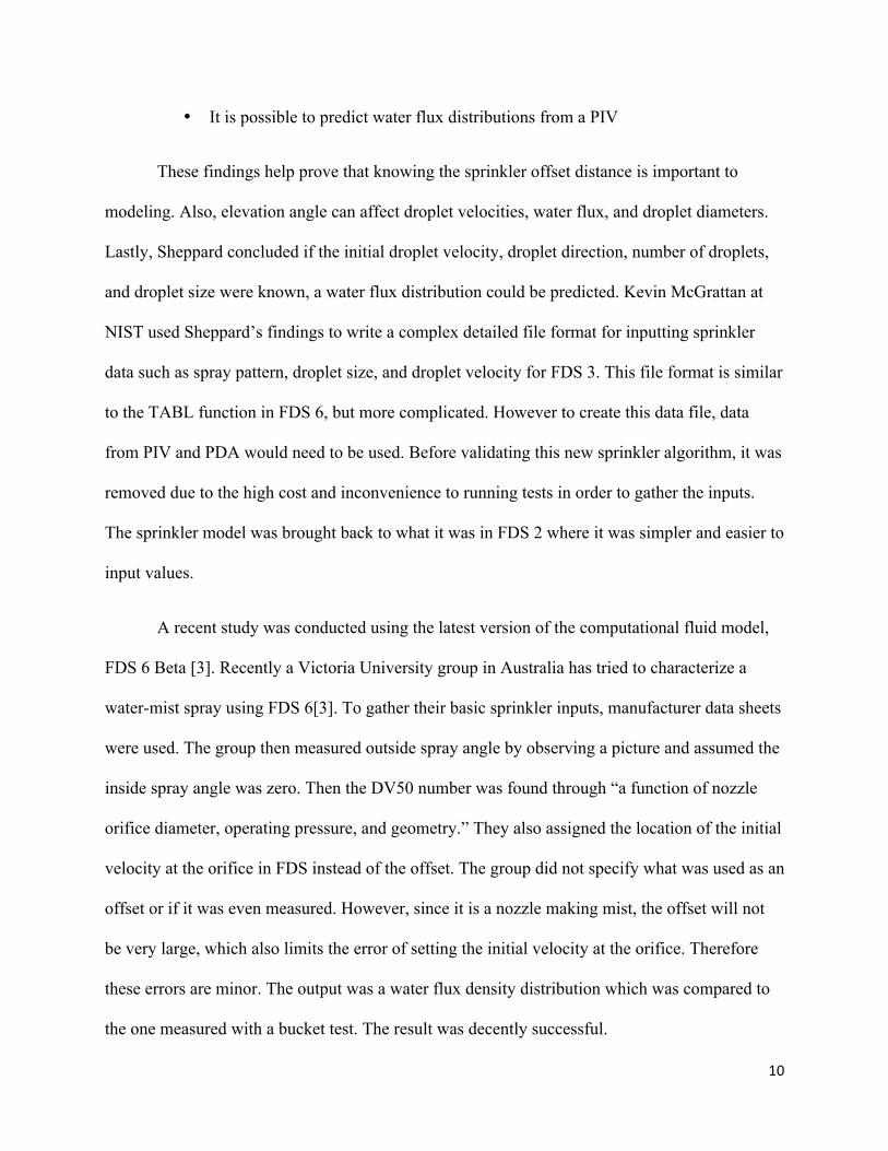
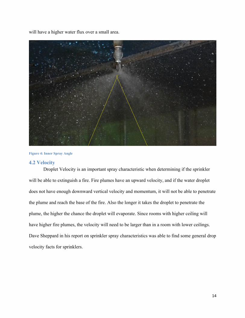
A main characteristic of the shape of spray of a sprinkler is the spray angle. There are two
different types of spray angles. There is an inner spray angle and an outer spray angle. The outer
spray angle is the angle of the outer boundaries of the spray. The inner spray angle is the
boundary of the area inside the spray where there is no water (figure 4). These spray angles
influence the spray distribution of water and governs the coverage. A lower outer spray angle
5
Orifice
Frame Arm
Deflector
Figure 2. Typical Sprinkler Design
Before the late 70’s most sprinklers were constructed with 12.7mm or 13.5mm
orifices and were designed to provide a flow rates in the range of 1.2 to 2.9 1sec−⋅� .
Research conducted in the 70’s and 80’s showed that specialized sprinklers could be
designed that were more effective in controlling certain types of fires. This research
stimulated a renaissance in sprinkler design, where many specialized sprinkler designs
were developed for special applications. Figure 3 shows schematically several different
sprinkler types.
Standard Pendant Early Suppression Fast Response
Traditional Upright Modern Upright
Figure 3. Sprinkler Examples
14
will have a higher water flux over a small area.
Figure 4: Inner Spray Angle
4.2 Velocity Droplet Velocity is an important spray characteristic when determining if the sprinkler
will be able to extinguish a fire. Fire plumes have an upward velocity, and if the water droplet
does not have enough downward vertical velocity and momentum, it will not be able to penetrate
the plume and reach the base of the fire. Also the longer it takes the droplet to penetrate the
plume, the higher the chance the droplet will evaporate. Since rooms with higher ceiling will
have higher fire plumes, the velocity will need to be larger than in a room with lower ceilings.
Dave Sheppard in his report on sprinkler spray characteristics was able to find some general drop
velocity facts for sprinklers.
15
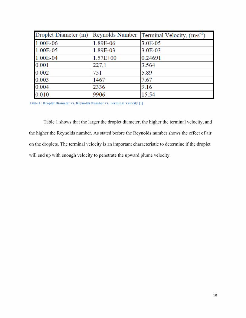
Table 1: Droplet Diameter vs. Reynolds Number vs. Terminal Velocity [1]
Table 1 shows that the larger the droplet diameter, the higher the terminal velocity, and
the higher the Reynolds number. As stated before the Reynolds number shows the effect of air
on the droplets. The terminal velocity is an important characteristic to determine if the droplet
will end up with enough velocity to penetrate the upward plume velocity.
16
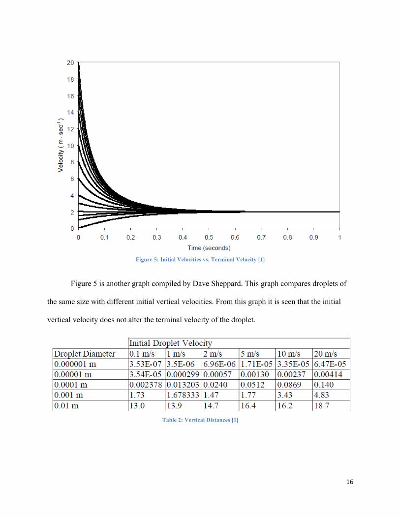
Figure 5: Initial Velocities vs. Terminal Velocity [1]
Figure 5 is another graph compiled by Dave Sheppard. This graph compares droplets of
the same size with different initial vertical velocities. From this graph it is seen that the initial
vertical velocity does not alter the terminal velocity of the droplet.
Table 2: Vertical Distances [1]
17
Table 2 above is a table showing the vertical distance it takes for different diameter
droplets to reach their terminal velocities at different initial droplet velocities. One finding is that
the larger the droplet, the farther the vertical distance to terminal velocity. Another finding is the
higher the initial droplet velocity, the farther the vertical distance to terminal velocity. An
average ten feet tall ceiling is approximately 3 meters. As you can see in this table a .01m droplet
would not reach its terminal velocity in this room. Therefore in a typical 10 feet tall room, a
smaller droplet would be more ideal for its cooling properties.
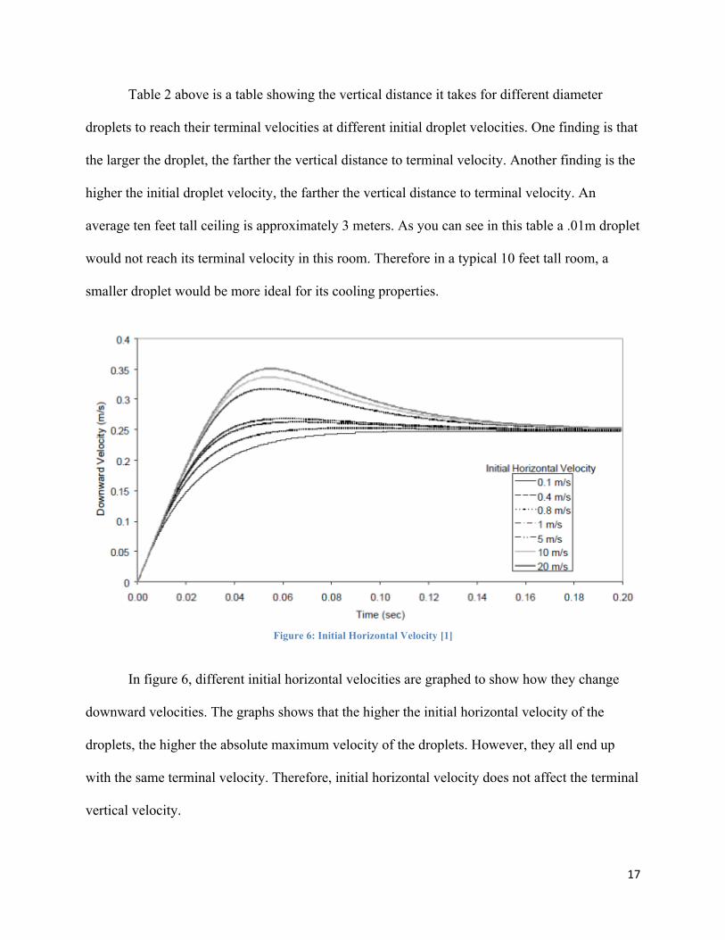
Figure 6: Initial Horizontal Velocity [1]
In figure 6, different initial horizontal velocities are graphed to show how they change
downward velocities. The graphs shows that the higher the initial horizontal velocity of the
droplets, the higher the absolute maximum velocity of the droplets. However, they all end up
with the same terminal velocity. Therefore, initial horizontal velocity does not affect the terminal
vertical velocity.
18
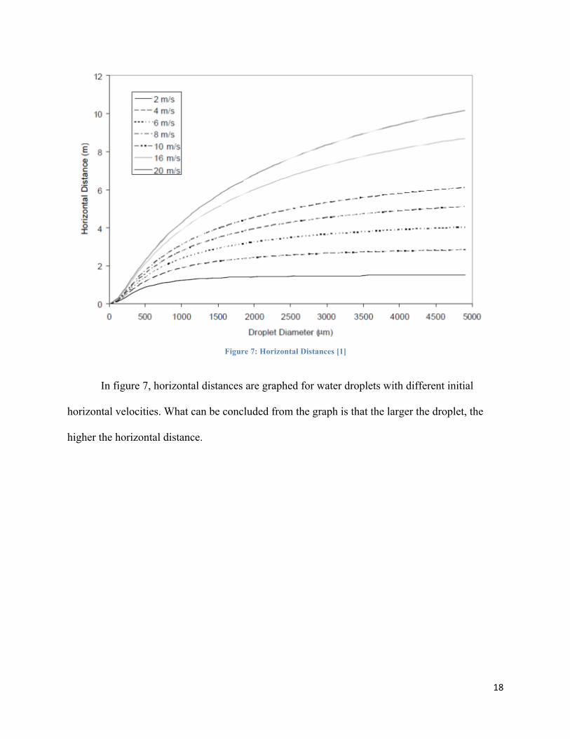
Figure 7: Horizontal Distances [1]
In figure 7, horizontal distances are graphed for water droplets with different initial
horizontal velocities. What can be concluded from the graph is that the larger the droplet, the
higher the horizontal distance.
19
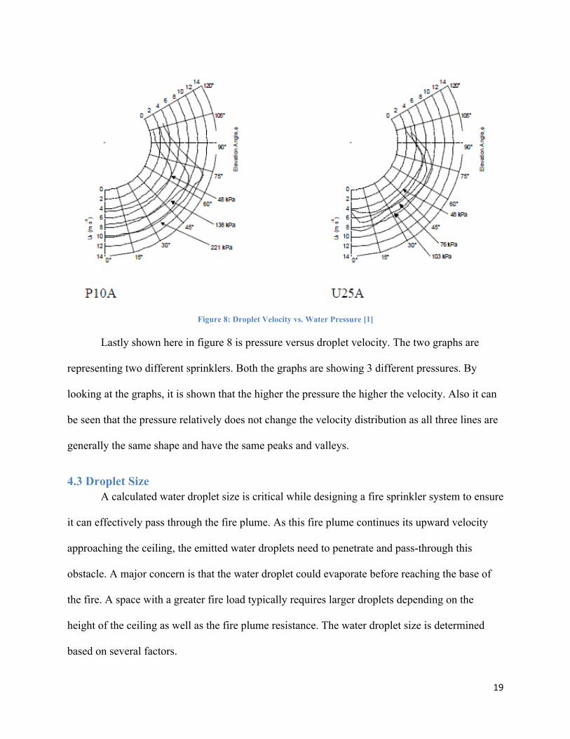
Figure 8: Droplet Velocity vs. Water Pressure [1]
Lastly shown here in figure 8 is pressure versus droplet velocity. The two graphs are
representing two different sprinklers. Both the graphs are showing 3 different pressures. By
looking at the graphs, it is shown that the higher the pressure the higher the velocity. Also it can
be seen that the pressure relatively does not change the velocity distribution as all three lines are
generally the same shape and have the same peaks and valleys.
4.3 Droplet Size A calculated water droplet size is critical while designing a fire sprinkler system to ensure
it can effectively pass through the fire plume. As this fire plume continues its upward velocity
approaching the ceiling, the emitted water droplets need to penetrate and pass-through this
obstacle. A major concern is that the water droplet could evaporate before reaching the base of
the fire. A space with a greater fire load typically requires larger droplets depending on the
height of the ceiling as well as the fire plume resistance. The water droplet size is determined
based on several factors.
20
First, there is a generally accepted correlation between pressure and water droplet size.
Typically higher the pressure the smaller the water droplets are. Pressure provided from the
water source may need to be altered to achieve the desired water droplet size.
Second is the deflector of the sprinkler head. The deflector is main differentiating factor
in choosing and designing a sprinkler system. Shape of the spray pattern, water-flux, and water
droplet size are dependent upon the deflector. The offset is the measure of distance from where
the water leaves the sprinkler head out of the orifice to the point where physical and individual
water droplets are formed after the atomization process. The deflector plays a key role in the
formation of water droplets by changing the water flow from a stream, to water sheets to water
droplets.
Lastly, location of the spray refers to the consistency of the water droplets within the
boundary of the coverage. There is a great variance of the water droplet distribution within the
shape of the spray pattern. Larger water droplet size is capable of greater velocity and farther
travel distance from the sprinkler head. An industry standard has been established for general
distribution patterns however in the field experimental testing is required to confidentially
understand actual distribution compared to expected distribution.
4.4 Water Flux The final characteristic is water flux of the fire sprinkler. Flux is a measure of volumetric
flow rate over the area. This is the amount of water that is discharged beneath the protected
sprinkler area. By determining the water flux it is possible to see how much water can be
delivered to the fire in order to extinguish it. The distribution of fluxes changes dramatically
when pressure is fluctuating. There is not a consistent water flux below the sprinkler coverage.

21
For example the water flux at the outer limits of the spray could be higher or lower than the flux
below the sprinkler depending on the type of sprinkler and pressure.
22
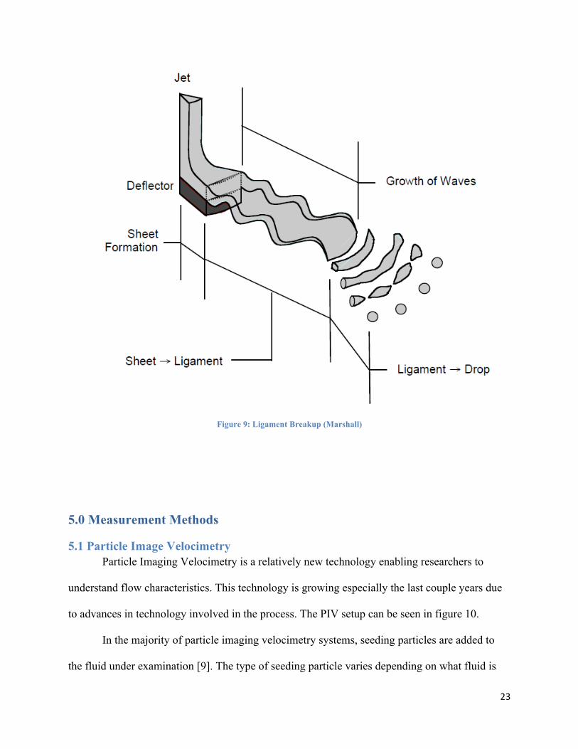
4.5 Spray Offset
Spray offset is a distance away from the sprinkler head in which atomization is complete,
forming droplets. Atomization is the process in which water droplets are created (Marshall).
There are three stages of atomization. They are sheet formation, sheet breakup, and ligament
breakup. The three stages are illustrated in figure 9. The first stage is sheet formation. The sheet
formation begins at the stagnation point where the water jet initially hits the deflector. When the
water jet collides with the deflector it forms a water sheet. This water sheet stays steady across
the deflector, but once the sheet leaves the deflector the second stage called sheet breakup
begins. Sheet breakup starts when the water sheet is no longer in contact with the deflector. The
sheet becomes unstable flowing through air and waves begin to form. These waves eventually
break up into ligaments. This is the beginning of the third stage named ligament breakup. In this
stage, waves once again are formed, however, this time they are formed in each individual
ligament. These waves cause break up again and form individual water droplets, completing the
process.
23
Figure 9: Ligament Breakup (Marshall)
5.0 Measurement Methods
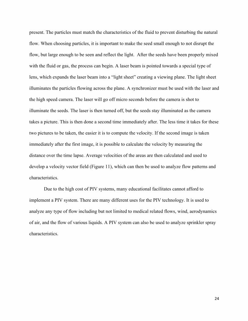
5.1 Particle Image Velocimetry Particle Imaging Velocimetry is a relatively new technology enabling researchers to
understand flow characteristics. This technology is growing especially the last couple years due
to advances in technology involved in the process. The PIV setup can be seen in figure 10.
In the majority of particle imaging velocimetry systems, seeding particles are added to
the fluid under examination [9]. The type of seeding particle varies depending on what fluid is
24
present. The particles must match the characteristics of the fluid to prevent disturbing the natural
flow. When choosing particles, it is important to make the seed small enough to not disrupt the
flow, but large enough to be seen and reflect the light. After the seeds have been properly mixed
with the fluid or gas, the process can begin. A laser beam is pointed towards a special type of
lens, which expands the laser beam into a “light sheet” creating a viewing plane. The light sheet
illuminates the particles flowing across the plane. A synchronizer must be used with the laser and
the high speed camera. The laser will go off micro seconds before the camera is shot to
illuminate the seeds. The laser is then turned off, but the seeds stay illuminated as the camera
takes a picture. This is then done a second time immediately after. The less time it takes for these
two pictures to be taken, the easier it is to compute the velocity. If the second image is taken
immediately after the first image, it is possible to calculate the velocity by measuring the
distance over the time lapse. Average velocities of the areas are then calculated and used to
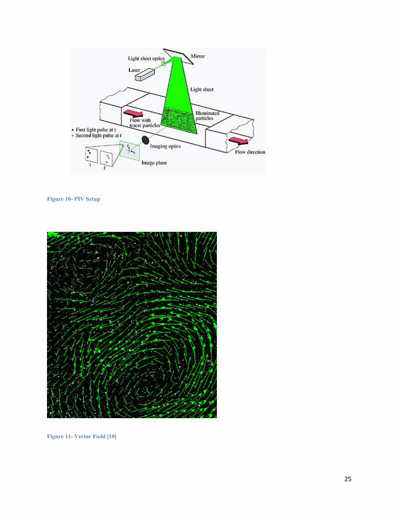
develop a velocity vector field (Figure 11), which can then be used to analyze flow patterns and
characteristics.
Due to the high cost of PIV systems, many educational facilitates cannot afford to
implement a PIV system. There are many different uses for the PIV technology. It is used to
analyze any type of flow including but not limited to medical related flows, wind, aerodynamics
of air, and the flow of various liquids. A PIV system can also be used to analyze sprinkler spray
characteristics.
25
Figure 10- PIV Setup
Figure 11- Vector Field [10]
26
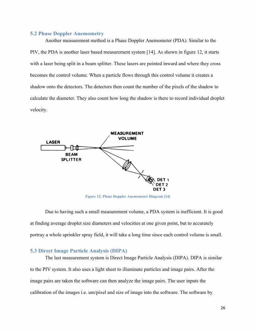
5.2 Phase Doppler Anemometry Another measurement method is a Phase Doppler Anemometer (PDA). Similar to the
PIV, the PDA is another laser based measurement system [14]. As shown in figure 12, it starts
with a laser being split in a beam splitter. These lasers are pointed inward and where they cross
becomes the control volume. When a particle flows through this control volume it creates a
shadow onto the detectors. The detectors then count the number of the pixels of the shadow to
calculate the diameter. They also count how long the shadow is there to record individual droplet
velocity.
Figure 12: Phase Doppler Anemometer Diagram [14]
Due to having such a small measurement volume, a PDA system is inefficient. It is good
at finding average droplet size diameters and velocities at one given point, but to accurately
portray a whole sprinkler spray field, it will take a long time since each control volume is small.
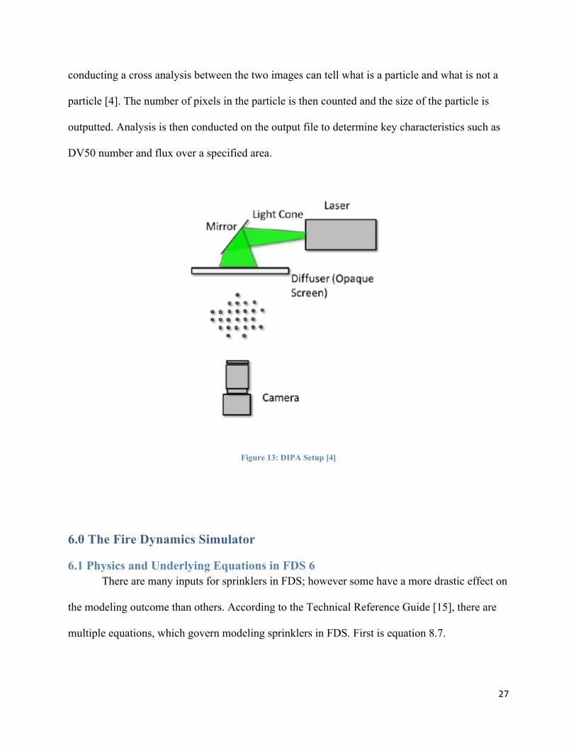
5.3 Direct Image Particle Analysis (DIPA) The last measurement system is Direct Image Particle Analysis (DIPA). DIPA is similar
to the PIV system. It also uses a light sheet to illuminate particles and image pairs. After the
image pairs are taken the software can then analyze the image pairs. The user inputs the
calibration of the images i.e. um/pixel and size of image into the software. The software by
27
conducting a cross analysis between the two images can tell what is a particle and what is not a
particle [4]. The number of pixels in the particle is then counted and the size of the particle is
outputted. Analysis is then conducted on the output file to determine key characteristics such as
DV50 number and flux over a specified area.
Figure 13: DIPA Setup [4]
6.0 The Fire Dynamics Simulator
6.1 Physics and Underlying Equations in FDS 6 There are many inputs for sprinklers in FDS; however some have a more drastic effect on
the modeling outcome than others. According to the Technical Reference Guide [15], there are
multiple equations, which govern modeling sprinklers in FDS. First is equation 8.7.
28
This equation states that the median droplet diameter is calculated with the orifice
diameter (D), and the Weber Number (We). Below is equation 8.8 from the Tech Guide, the
Weber Number.
The Weber Number is a function of droplet density (ρd), discharge velocity (ud), and
liquid surface tension (σd, 72.8*10^-3 N/m for water at 20 0C, default). FDS attempts to track
changes in pressure and use these changes to the track droplet boundary conditions. Below are
equations 8.9, 8.10, ands 8.11 that FDS uses for mass flow, droplet speed, and median diameter.
These equations mean that the mass flow, discharge velocity and median diameter are
proportional to functions of pressure.
6.1.1 Number of Particles The FDS 6 user guide states that a sprinkler creates more droplets in a second than what
FDS can replicate (User Guide, section 14.5.2) [16]. As a result, FDS 6 uses one particle to track
the movement of a group of particles. To specify the number of particles that is introduced per
second, the PROP line is used:
PARTICLES_PER_SECOND (Default is 5000)
A large number of particles can cause the model to be unstable. However, larger number
of droplets can yield more accurate mass flux distributions. Therefore a sensitivity analysis needs
to be conducted for particles per second when modeling sprinklers.
29
6.1.2 Particle Size Distribution Another parameter to input into FDS is DROPLET DIAMETER. FDS then uses this
value to distribute droplet size in one of three different ways. These distributions are listed
below:
ROSIN-RAMMLER-LOGNORMAL
The Rosin-Rammler-Lognormal is the default distribution used in FDS 6. Research at
FM has suggested that the Cumulative Volume Fraction (CVF) can be represented by
using a combination of log-normal and Rosin-Rammler distributions. These relationships
can be seen below:
In the equation, dm is the mean droplet diameter. Then σ and γ are empirical constants,
which are 0.6 and 2.4 by default. When the droplet diameter is less than or equal to the
mean droplet diameter, the lognormal distribution is used. When the droplet diameter is
greater than the mean diameter, the Rosin-Rammler distribution is used. In FDS 6, the
Lognormal and Rosin-Rammler distributions can be used independently to predict the
CVF as well.
LOGNORMAL
ROSIN-RAMMLER
30
6.2 Limitations One of the known limitations of FDS is the cell size. When setting up an FDS simulation,
one needs to keep in mind how many cells to create and the size of each cell. The more cells
added, the longer the simulation will take to run. However, more cells do not necessarily mean
greater accuracy. When setting up an FDS file, different number of cells needs to be tested.
However, when trying to set up precise experiments in FDS, rounding will need to take place.
For example, an order of millimeters might not be possible in FDS; therefore the experiment will
need to be measured to the nearest centimeter.
Another limitation in FDS is the effect of the deflector. Deflectors vary between different
types of sprinklers. An extended coverage sprinkler will have a different deflector than a
residential sprinkler. To account for this limitation, FDS sprinkler modeling tries to characterize
the spray after it hits the deflector and the spray is formed. FDS sprinkler modeling ignores the
beginning stages of the atomization process.
31
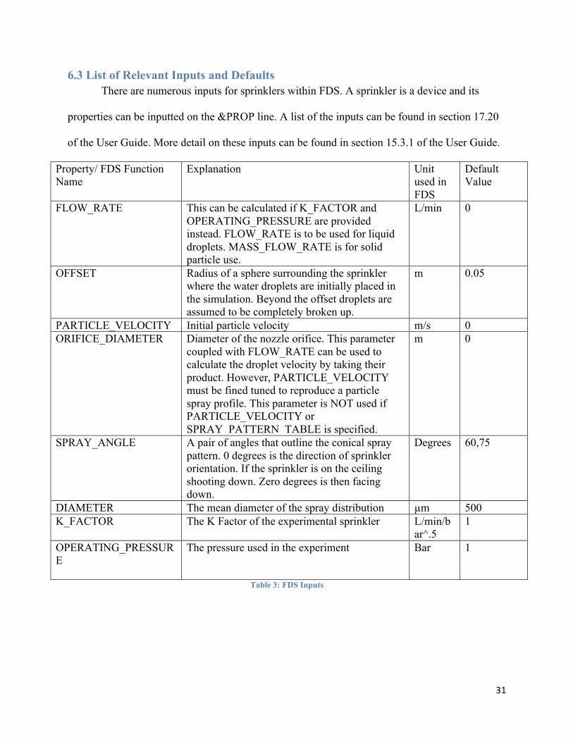
6.3 List of Relevant Inputs and Defaults There are numerous inputs for sprinklers within FDS. A sprinkler is a device and its
properties can be inputted on the &PROP line. A list of the inputs can be found in section 17.20
of the User Guide. More detail on these inputs can be found in section 15.3.1 of the User Guide.
Property/ FDS Function Name
Explanation Unit used in FDS
Default Value
FLOW_RATE This can be calculated if K_FACTOR and OPERATING_PRESSURE are provided instead. FLOW_RATE is to be used for liquid droplets. MASS_FLOW_RATE is for solid particle use.
L/min 0
OFFSET Radius of a sphere surrounding the sprinkler where the water droplets are initially placed in the simulation. Beyond the offset droplets are assumed to be completely broken up.
m 0.05
PARTICLE_VELOCITY Initial particle velocity m/s 0 ORIFICE_DIAMETER Diameter of the nozzle orifice. This parameter
coupled with FLOW_RATE can be used to calculate the droplet velocity by taking their product. However, PARTICLE_VELOCITY must be fined tuned to reproduce a particle spray profile. This parameter is NOT used if PARTICLE_VELOCITY or SPRAY_PATTERN_TABLE is specified.
m 0
SPRAY_ANGLE A pair of angles that outline the conical spray pattern. 0 degrees is the direction of sprinkler orientation. If the sprinkler is on the ceiling shooting down. Zero degrees is then facing down.
Degrees 60,75
DIAMETER The mean diameter of the spray distribution µm 500 K_FACTOR
The K Factor of the experimental sprinkler L/min/bar^.5
1
OPERATING_PRESSURE
The pressure used in the experiment Bar 1
Table 3: FDS Inputs
32
7.0 Characterization of Upright Extended Coverage k-25.2 Fire Sprinkler
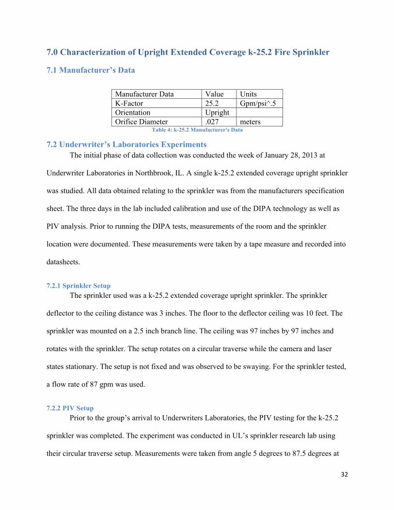
7.1 Manufacturer’s Data
Manufacturer Data Value Units K-Factor 25.2 Gpm/psi^.5 Orientation Upright Orifice Diameter .027 meters
Table 4: k-25.2 Manufacturer's Data
7.2 Underwriter’s Laboratories Experiments The initial phase of data collection was conducted the week of January 28, 2013 at
Underwriter Laboratories in Northbrook, IL. A single k-25.2 extended coverage upright sprinkler
was studied. All data obtained relating to the sprinkler was from the manufacturers specification
sheet. The three days in the lab included calibration and use of the DIPA technology as well as
PIV analysis. Prior to running the DIPA tests, measurements of the room and the sprinkler
location were documented. These measurements were taken by a tape measure and recorded into
datasheets.
7.2.1 Sprinkler Setup The sprinkler used was a k-25.2 extended coverage upright sprinkler. The sprinkler
deflector to the ceiling distance was 3 inches. The floor to the deflector ceiling was 10 feet. The
sprinkler was mounted on a 2.5 inch branch line. The ceiling was 97 inches by 97 inches and
rotates with the sprinkler. The setup rotates on a circular traverse while the camera and laser
states stationary. The setup is not fixed and was observed to be swaying. For the sprinkler tested,
a flow rate of 87 gpm was used.
7.2.2 PIV Setup Prior to the group’s arrival to Underwriters Laboratories, the PIV testing for the k-25.2
sprinkler was completed. The experiment was conducted in UL’s sprinkler research lab using
their circular traverse setup. Measurements were taken from angle 5 degrees to 87.5 degrees at
33
every 2.5 degrees totaling in measurements at 34 different angles. Measurements could not be
made at 0 degrees because the rotating pipe assembly blocks the camera. Measurements at 90
degrees could also not be taken because the rotating pipe assembly blocks the laser sheet. For
each angle 150 image pairs were taken. The camera took each image 150 µs apart. The images
were calibrated at 5 degrees, 15 degrees, 30 degrees, 45 degrees, 60 degrees, and 75 degrees.
Then using the Insight 3g software, all 150 image pairs were analyzed to produce a velocity
vector map and an excel output file. Each vector was outputted with x,y coordinates and velocity
in x and y direction.
7.2.3 DIPA Setup The group was able to observe and conduct the DIPA experiment during their trip. The
experiment was completed in UL’s sprinkler research lab using their circular traverse setup.
Measurements were taken from angle 5 degrees to 87.5 degrees at every 2.5 degrees totaling in
34 angles. Measurements could not be made at 0 degrees because the rotating pipe assembly
blocks the camera. Measurements at 90 degrees could also not be taken because the rotating pipe
assembly blocks the laser sheet. For each angle 150 image pairs were taken. The camera takes
each image 150 µs apart. The images were calibrated at 5 degrees, 15 degrees, 30 degrees, 45
degrees, 60 degrees, and 75 degrees. 4 different image sets were taken. There was one with an
origin at 0, 0 (at the sprinkler), 8, 0(8 inches to the right of the sprinkler), 0, 8(8 inches below the
sprinkler) and 8, 8(8 inches below and 8 inches to the right of the sprinkler). During the group’s
time, only data for (8, 0) was analyzed at 15 degrees. Using the insight 3g software, all 150
image pairs were analyzed to measured droplet size data.
34
7.3 Measured Model Inputs
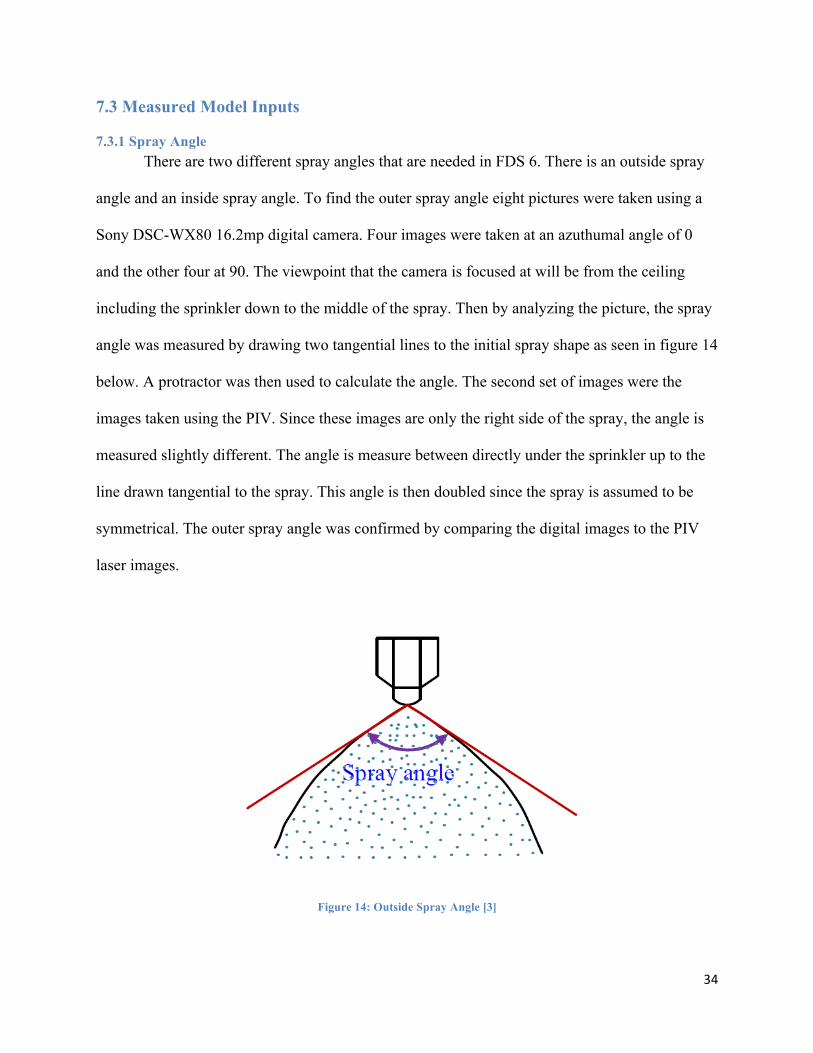
7.3.1 Spray Angle There are two different spray angles that are needed in FDS 6. There is an outside spray
angle and an inside spray angle. To find the outer spray angle eight pictures were taken using a
Sony DSC-WX80 16.2mp digital camera. Four images were taken at an azuthumal angle of 0
and the other four at 90. The viewpoint that the camera is focused at will be from the ceiling
including the sprinkler down to the middle of the spray. Then by analyzing the picture, the spray
angle was measured by drawing two tangential lines to the initial spray shape as seen in figure 14
below. A protractor was then used to calculate the angle. The second set of images were the
images taken using the PIV. Since these images are only the right side of the spray, the angle is
measured slightly different. The angle is measure between directly under the sprinkler up to the
line drawn tangential to the spray. This angle is then doubled since the spray is assumed to be
symmetrical. The outer spray angle was confirmed by comparing the digital images to the PIV
laser images.
Figure 14: Outside Spray Angle [3]
35
Once the 8 images were analyzed, the 8 spray angles were averaged to find the final
average outer spray angle. The inside spray angle was measured by analyzing the PIV laser
images. At each calibrated angle, the PIV laser image was analyzed to measure the inner spray
angle. If there is an inside spray angle visible in the image, it will be measured using protractor,
but if there is no visible inside spray angle, the inside spray angle is assumed to be zero.
The average spray angle found from the digital camera images was 150.11 degrees. The
PIV laser images were analyzed and an average angle of 147.14 degrees was measured. This
resulted in a 2% difference between the digital camera and the PIV images. This small difference
means expensive technology is not needed to measure spray angle. All that is needed is a
sprinkler set up and a digital camera.
7.3.2 Droplet Size In FDS 6, particle sizes follow one out of three selected distributions:
• Rosin-Rammler-Lognormal Distribution
• Rosin-Rammler Distribution
• Lognormal Distribution
The default distribution is the Rosin-Rammler-Lognormal distribution. This combination
uses two distributions by utilizing the Rosin-Rammler method up until the median volumetric
diameter (DV50) where it then switches to the Lognormal distribution when droplets are greater
than the median. For FDS to utilize these distributions, the DV50 number needs to be specified.
Analysis was conducted with the DIPA data at 15 degrees. Due to time constraints, only a single
angle of 15 degrees was analyzed. Since such a small sample size was analyzed and the DIPA
technology has not been validated, historical droplet sizes were researched. A former UL test on
a similar k-25.2 upright sprinkler found that the mean volumetric diameter was 1161 microns.
36
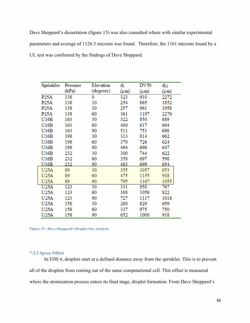
Dave Sheppard’s dissertation (figure 15) was also consulted where with similar experimental
parameters and average of 1126.3 microns was found. Therefore, the 1161 microns found by a
UL test was confirmed by the findings of Dave Sheppard.
Figure 15 - Dave Sheppard's Droplet Size Analysis
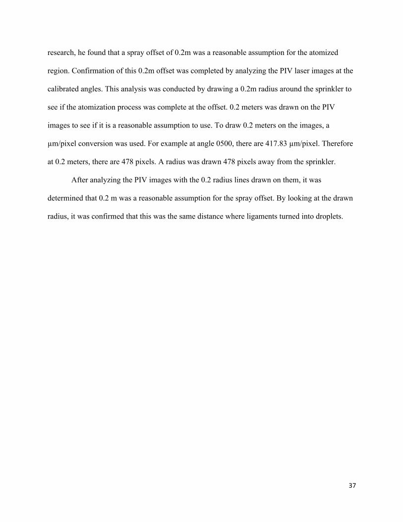
7.3.3 Spray Offset In FDS 6, droplets start at a defined distance away from the sprinkler. This is to prevent
all of the droplets from coming out of the same computational cell. This offset is measured
where the atomization process enters its final stage, droplet formation. From Dave Sheppard’s
37
research, he found that a spray offset of 0.2m was a reasonable assumption for the atomized
region. Confirmation of this 0.2m offset was completed by analyzing the PIV laser images at the
calibrated angles. This analysis was conducted by drawing a 0.2m radius around the sprinkler to
see if the atomization process was complete at the offset. 0.2 meters was drawn on the PIV
images to see if it is a reasonable assumption to use. To draw 0.2 meters on the images, a
µm/pixel conversion was used. For example at angle 0500, there are 417.83 µm/pixel. Therefore
at 0.2 meters, there are 478 pixels. A radius was drawn 478 pixels away from the sprinkler.
After analyzing the PIV images with the 0.2 radius lines drawn on them, it was
determined that 0.2 m was a reasonable assumption for the spray offset. By looking at the drawn
radius, it was confirmed that this was the same distance where ligaments turned into droplets.
38
Figure 16: Spray Offset at 15 Degrees
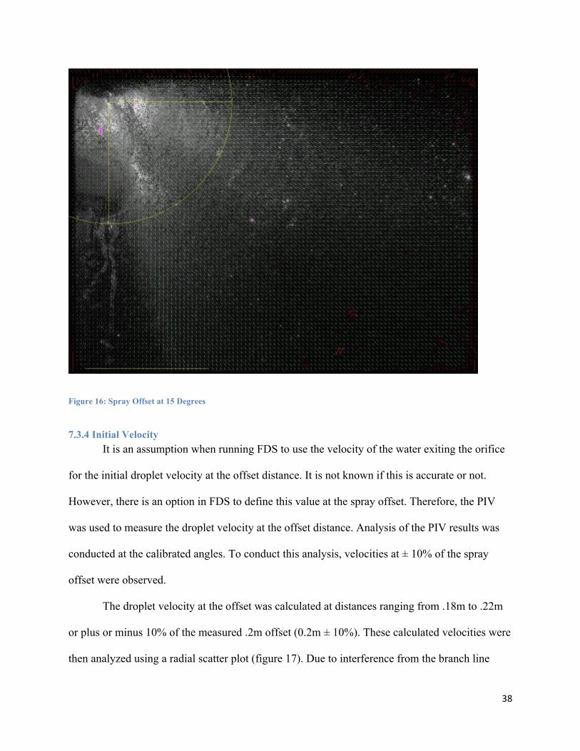
7.3.4 Initial Velocity It is an assumption when running FDS to use the velocity of the water exiting the orifice
for the initial droplet velocity at the offset distance. It is not known if this is accurate or not.
However, there is an option in FDS to define this value at the spray offset. Therefore, the PIV
was used to measure the droplet velocity at the offset distance. Analysis of the PIV results was
conducted at the calibrated angles. To conduct this analysis, velocities at ± 10% of the spray
offset were observed.
The droplet velocity at the offset was calculated at distances ranging from .18m to .22m
or plus or minus 10% of the measured .2m offset (0.2m ± 10%). These calculated velocities were
then analyzed using a radial scatter plot (figure 17). Due to interference from the branch line
39
velocities from 0 degrees to 20 degrees were not included in the calculation of the average
velocity. By averaging the velocities from 20 degrees to 90 degrees an average droplet velocity
at the 0.2m offset was determined to be 8.65 m/s.
Figure 17: Velocity Radial Scatter Plot
8.0 Characterization of Pendant k5.6 Sprinkler
Manufacturer Data Value Units K-Factor 5.6 Gpm/psi^.5 Orientation Pendant Orifice Diameter .0127 meters
Table 5: k-5.6 Manufacturer's Data
8.1 Measured Model Inputs
8.1.1 Spray Angle Spray angle was measured the same for the k5.6 sprinkler as it was in for the k25.2
sprinkler by using a protractor on digital images. To find the outer spray angle, images were
taken using a Sony DSC-WX80 16.2mp digital camera during bucket tests conducted at Tyco.
0
2
4
6
8
10
12
-‐40 -‐20 0 20 40 60 80 100 120
Drop
let V
elocity
(m/s)
Spray Angle (Degrees)
45 Degrees
Droplet Velocity
40
Three angles were found from three images and were averaged. The resulting outer spray angle
was 145.25 degrees. To find the inner spray angle, more images were analyzed. The average of
three angles resulted in an inner spray angle of 46 degrees.
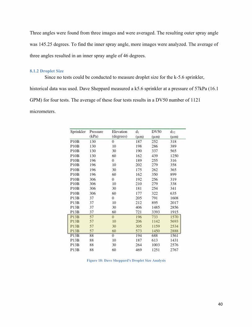
8.1.2 Droplet Size Since no tests could be conducted to measure droplet size for the k-5.6 sprinkler,
historical data was used. Dave Sheppard measured a k5.6 sprinkler at a pressure of 57kPa (16.1
GPM) for four tests. The average of these four tests results in a DV50 number of 1121
micrometers.
Figure 18: Dave Sheppard's Droplet Size Analysis
41
8.1.3 Spray Offset Once again, since offset could not be measured for the k5.6 sprinkler, historical data was
used. Sheppard states in his dissertation that of 0.2m was a reasonable assumption for the
atomized region. Therefore 0.2 meters was used as the offset distance for the k5.6 sprinkler.
There were no PIV data for this sprinkler; therefore the group was no able to check the offset
distance.
8.1.4 Initial Velocity Since no PIV tests were run on the k5.6 sprinkler, velocity could not be measured at the
offset. Velocity was then calculated at the orifice using the equation.
𝑉 =4𝑄𝜋𝑑!
Where v is velocity, Q is flow rate, and d is orifice diameter. The orifice diameter for the
sprinkler was .0127 meters, the flow rate was 15 gallons per minute and the resulting velocity at
the orifice was 7.4 meters per second
9.0 Prediction of Actual Delivered Density (ADD) with FDS and Comparison to Measured ADD for K25.2 Sprinkler
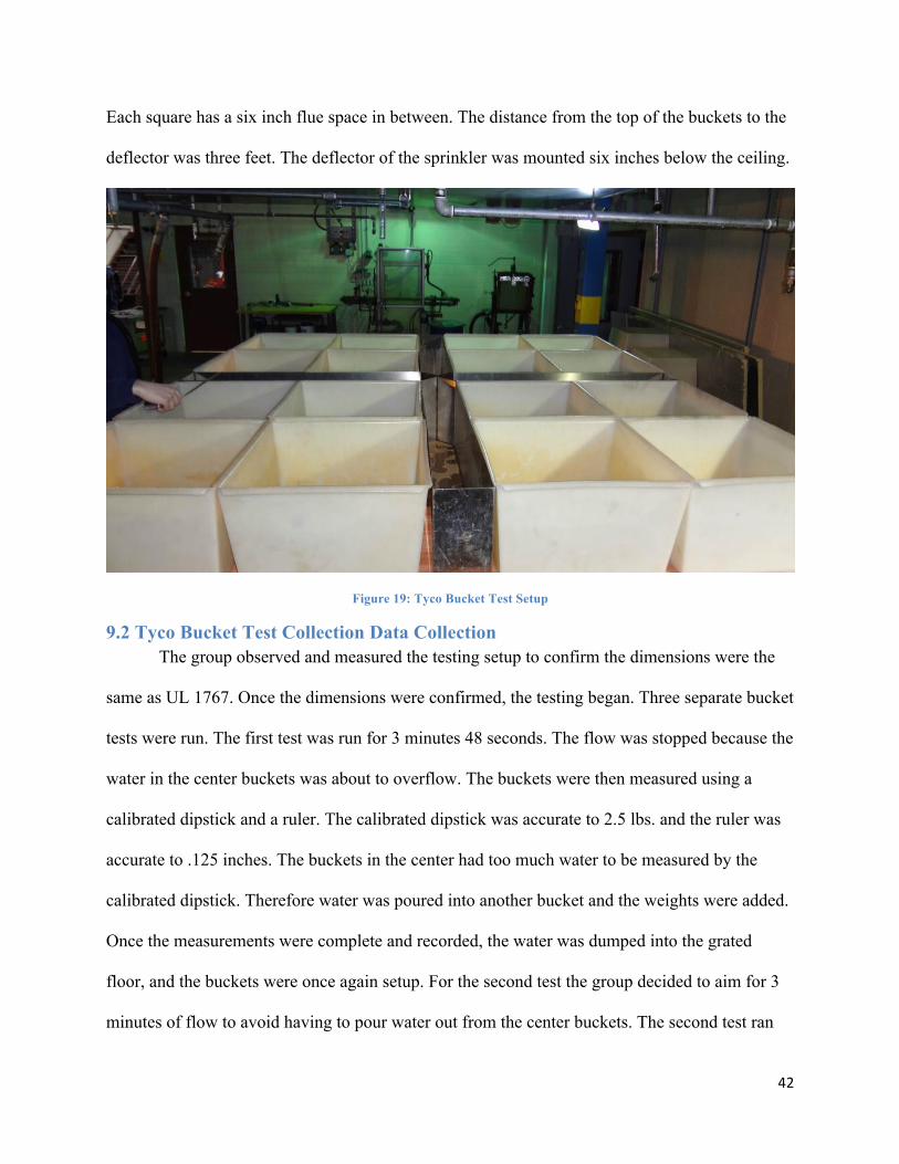
9.1 Tyco Experiments Water flux rather than an input or initial characteristic, is an output in FDS. To validate
the experiment and verify the four main inputs, water flux distribution in FDS was used. To
measure the flux distribution, a bucket test was used. On February 21, 2013, the project group
went to Cranston, Rhode Island to conduct bucket tests of the k-25.2 upright sprinkler at Tyco’s
Sprinkler Research Lab. The bucket test conducted at Tyco was setup to the dimensions of the
ADD test in UL Standard 1767. There were 16 buckets set up below the sprinkler. Each bucket
was .5 meters by .5 meters. The buckets were setup up in 4 squares each one meter by one meter.
42
Each square has a six inch flue space in between. The distance from the top of the buckets to the
deflector was three feet. The deflector of the sprinkler was mounted six inches below the ceiling.
Figure 19: Tyco Bucket Test Setup
9.2 Tyco Bucket Test Collection Data Collection The group observed and measured the testing setup to confirm the dimensions were the
same as UL 1767. Once the dimensions were confirmed, the testing began. Three separate bucket
tests were run. The first test was run for 3 minutes 48 seconds. The flow was stopped because the
water in the center buckets was about to overflow. The buckets were then measured using a
calibrated dipstick and a ruler. The calibrated dipstick was accurate to 2.5 lbs. and the ruler was
accurate to .125 inches. The buckets in the center had too much water to be measured by the
calibrated dipstick. Therefore water was poured into another bucket and the weights were added.
Once the measurements were complete and recorded, the water was dumped into the grated
floor, and the buckets were once again setup. For the second test the group decided to aim for 3
minutes of flow to avoid having to pour water out from the center buckets. The second test ran
43
for exactly 3 minutes and the measuring process was conducted again. The third test ran for 3
minutes 1 second.
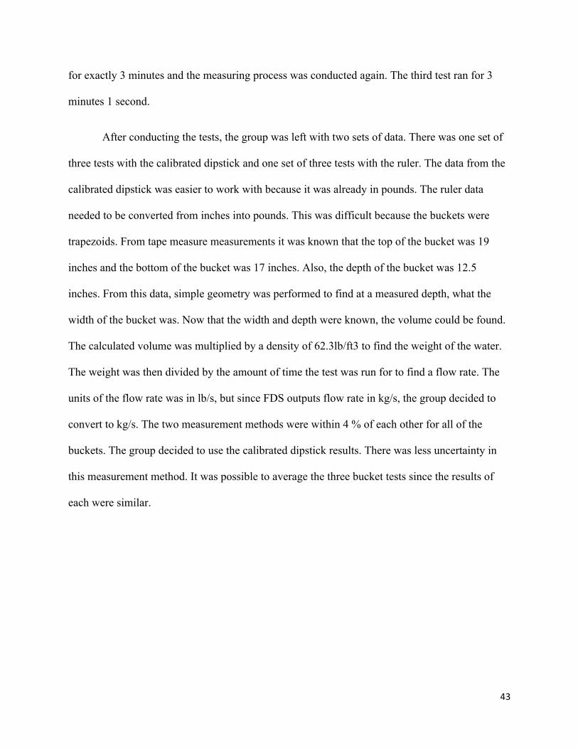
After conducting the tests, the group was left with two sets of data. There was one set of
three tests with the calibrated dipstick and one set of three tests with the ruler. The data from the
calibrated dipstick was easier to work with because it was already in pounds. The ruler data
needed to be converted from inches into pounds. This was difficult because the buckets were
trapezoids. From tape measure measurements it was known that the top of the bucket was 19
inches and the bottom of the bucket was 17 inches. Also, the depth of the bucket was 12.5
inches. From this data, simple geometry was performed to find at a measured depth, what the
width of the bucket was. Now that the width and depth were known, the volume could be found.
The calculated volume was multiplied by a density of 62.3lb/ft3 to find the weight of the water.
The weight was then divided by the amount of time the test was run for to find a flow rate. The
units of the flow rate was in lb/s, but since FDS outputs flow rate in kg/s, the group decided to
convert to kg/s. The two measurement methods were within 4 % of each other for all of the
buckets. The group decided to use the calibrated dipstick results. There was less uncertainty in
this measurement method. It was possible to average the three bucket tests since the results of
each were similar.
44
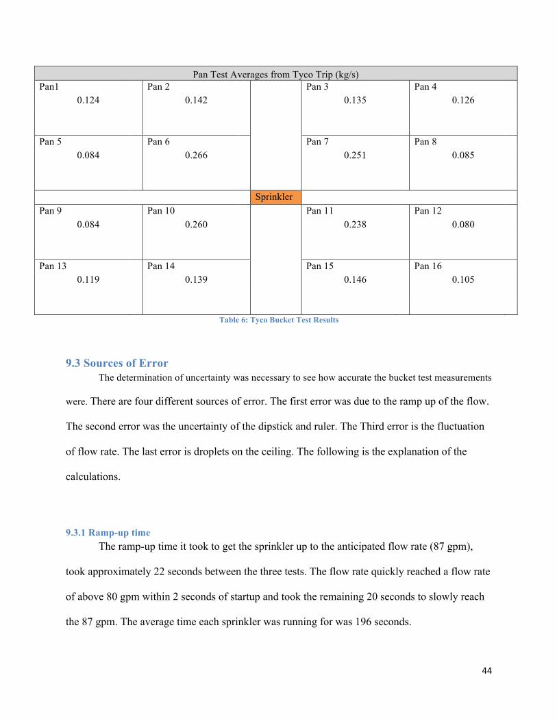
Pan Test Averages from Tyco Trip (kg/s) Pan1 Pan 2 Pan 3 Pan 4
0.124 0.142 0.135 0.126 Pan 5 Pan 6 Pan 7 Pan 8
0.084 0.266 0.251 0.085 Sprinkler Pan 9 Pan 10 Pan 11 Pan 12
0.084 0.260 0.238 0.080 Pan 13 Pan 14 Pan 15 Pan 16
0.119 0.139 0.146 0.105
Table 6: Tyco Bucket Test Results
9.3 Sources of Error The determination of uncertainty was necessary to see how accurate the bucket test measurements
were. There are four different sources of error. The first error was due to the ramp up of the flow.
The second error was the uncertainty of the dipstick and ruler. The Third error is the fluctuation
of flow rate. The last error is droplets on the ceiling. The following is the explanation of the
calculations.
9.3.1 Ramp-up time The ramp-up time it took to get the sprinkler up to the anticipated flow rate (87 gpm),
took approximately 22 seconds between the three tests. The flow rate quickly reached a flow rate
of above 80 gpm within 2 seconds of startup and took the remaining 20 seconds to slowly reach
the 87 gpm. The average time each sprinkler was running for was 196 seconds.
45
0-2 seconds: 0 gpm -80 gpm (assumed average of 40 gpm over time: 0 -2 seconds)
3-22 seconds: 80 gpm – 87 gpm (assumed average of 83.5 gpm over time: 3 -22 seconds)
(2/24seconds)* (40gpm) + (22/24 seconds) * (83.5gpm) = 79.875 gpm
Therefore the average flow rate during the “ramp-up” process was 79.875 gpm.
Ramp-up: 0 – 22 seconds: 79.875 gpm
Steady-state: 23- 196 seconds: 87 gpm (ideal)
Uncertainty:
Ramp-up time * (Steady-state (gpm) – Ramp-up (gpm)) Total time Steady-state (gpm) = (22/196 seconds) * (87 – 79.875)/ 87 = 0.91% ±0.91 %
9.3.2 Measurement techniques The calibrated dipstick provided by Tyco was made up of 2.5 lb increments spanning
from 5lbs to 120lbs. To calculate the uncertainty of measurement errors, an average of 75lbs was
used as the base value to cover the majority of the magnitude of measurements captured at Tyco.
= Uncertainty in measurement Base Value
= 1.25lbs / 75lbs = 1.67% ±1.67 %
9.3.3 Fluctuating flow rate The flow rate, after reaching steady state at 87 gpm, still continued to fluctuate from
measurements of 86.6 gpm to a maximum of 87.5 gpm. A range of 0.9 gpm was seen with the
sprinkler at the desired 87 gpm.
Uncertainty: = Uncertainty in measurement
Base Value
46
= 0.5gpm / 87gpm = 0.57 % ±0.57%
9.3.4 Ceiling effects The uncertainty of the ceiling playing a role in affecting the water distribution into the
buckets is unknown, so a large percent error was used to account for this factor:
±5%
9.3.5 Total Uncertainty: = Ramp-up time + measurement techniques + fluctuating flow rate + ceiling effects
= (±0.91%) + (±1.67%) + (±0.57%) + (±5%)
Total Uncertainty:
= ±8.15 %
10.0 Prediction of Actual Delivered Density (ADD) with FDS and Comparison to Measured ADD for k5.6 Sprinkler
10.1 Tyco Experiments A second water flux distribution comparison was completed to see if a different sprinkler
would increase or decrease the predictive capability. To validate the experiment and verify the
four main inputs, water flux distribution in FDS was used. To measure the flux distribution, a
bucket test was used. On April 12, 2013, the project group went to Cranston, Rhode Island to
conduct bucket tests of the k-5.6 pendent sprinkler at Tyco’s Sprinkler Research Lab. A similar
bucket test setup was used as the k-25.2 sprinkler. There were 16 buckets set up below the
sprinkler. Each bucket was .5 meters by .5 meters. The buckets were setup up in 4 squares each
one meter by one meter. Each square has a six inch flue space in between. The distance from the
top of the buckets to the deflector was three feet. The deflector of the sprinkler was mounted six
inches below the ceiling.
47
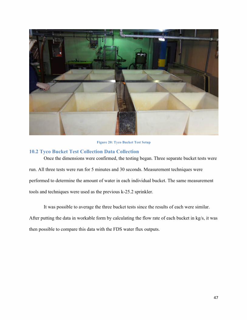
Figure 20: Tyco Bucket Test Setup
10.2 Tyco Bucket Test Collection Data Collection Once the dimensions were confirmed, the testing began. Three separate bucket tests were
run. All three tests were run for 5 minutes and 30 seconds. Measurement techniques were
performed to determine the amount of water in each individual bucket. The same measurement
tools and techniques were used as the previous k-25.2 sprinkler.
It was possible to average the three bucket tests since the results of each were similar.
After putting the data in workable form by calculating the flow rate of each bucket in kg/s, it was
then possible to compare this data with the FDS water flux outputs.
48
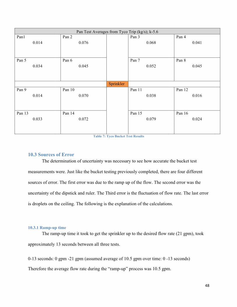
Pan Test Averages from Tyco Trip (kg/s); k-5.6 Pan1 Pan 2 Pan 3 Pan 4
0.014 0.076 0.068 0.041 Pan 5 Pan 6 Pan 7 Pan 8
0.034 0.045 0.052 0.045 Sprinkler Pan 9 Pan 10 Pan 11 Pan 12
0.014 0.070 0.038 0.016 Pan 13 Pan 14 Pan 15 Pan 16
0.033 0.072 0.079 0.024
Table 7: Tyco Bucket Test Results
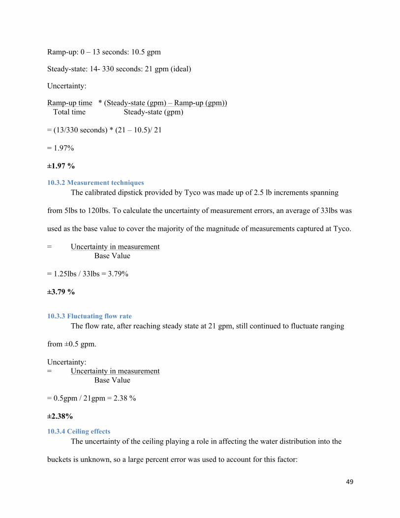
10.3 Sources of Error The determination of uncertainty was necessary to see how accurate the bucket test
measurements were. Just like the bucket testing previously completed, there are four different
sources of error. The first error was due to the ramp up of the flow. The second error was the
uncertainty of the dipstick and ruler. The Third error is the fluctuation of flow rate. The last error
is droplets on the ceiling. The following is the explanation of the calculations.
10.3.1 Ramp-up time The ramp-up time it took to get the sprinkler up to the desired flow rate (21 gpm), took
approximately 13 seconds between all three tests.
0-13 seconds: 0 gpm -21 gpm (assumed average of 10.5 gpm over time: 0 -13 seconds)
Therefore the average flow rate during the “ramp-up” process was 10.5 gpm.
49
Ramp-up: 0 – 13 seconds: 10.5 gpm
Steady-state: 14- 330 seconds: 21 gpm (ideal)
Uncertainty:
Ramp-up time * (Steady-state (gpm) – Ramp-up (gpm)) Total time Steady-state (gpm) = (13/330 seconds) * (21 – 10.5)/ 21 = 1.97% ±1.97 %
10.3.2 Measurement techniques The calibrated dipstick provided by Tyco was made up of 2.5 lb increments spanning
from 5lbs to 120lbs. To calculate the uncertainty of measurement errors, an average of 33lbs was
used as the base value to cover the majority of the magnitude of measurements captured at Tyco.
= Uncertainty in measurement Base Value
= 1.25lbs / 33lbs = 3.79% ±3.79 %
10.3.3 Fluctuating flow rate The flow rate, after reaching steady state at 21 gpm, still continued to fluctuate ranging
from ±0.5 gpm.
Uncertainty: = Uncertainty in measurement
Base Value = 0.5gpm / 21gpm = 2.38 % ±2.38%
10.3.4 Ceiling effects The uncertainty of the ceiling playing a role in affecting the water distribution into the
buckets is unknown, so a large percent error was used to account for this factor:
50
±5%
10.3.5 Total Uncertainty: = Ramp-up time + measurement techniques + fluctuating flow rate + ceiling effects
= (±1.97%) + (±3.79%) + (±2.38%) + (±5%)
Total Uncertainty:
= ±13.14 %
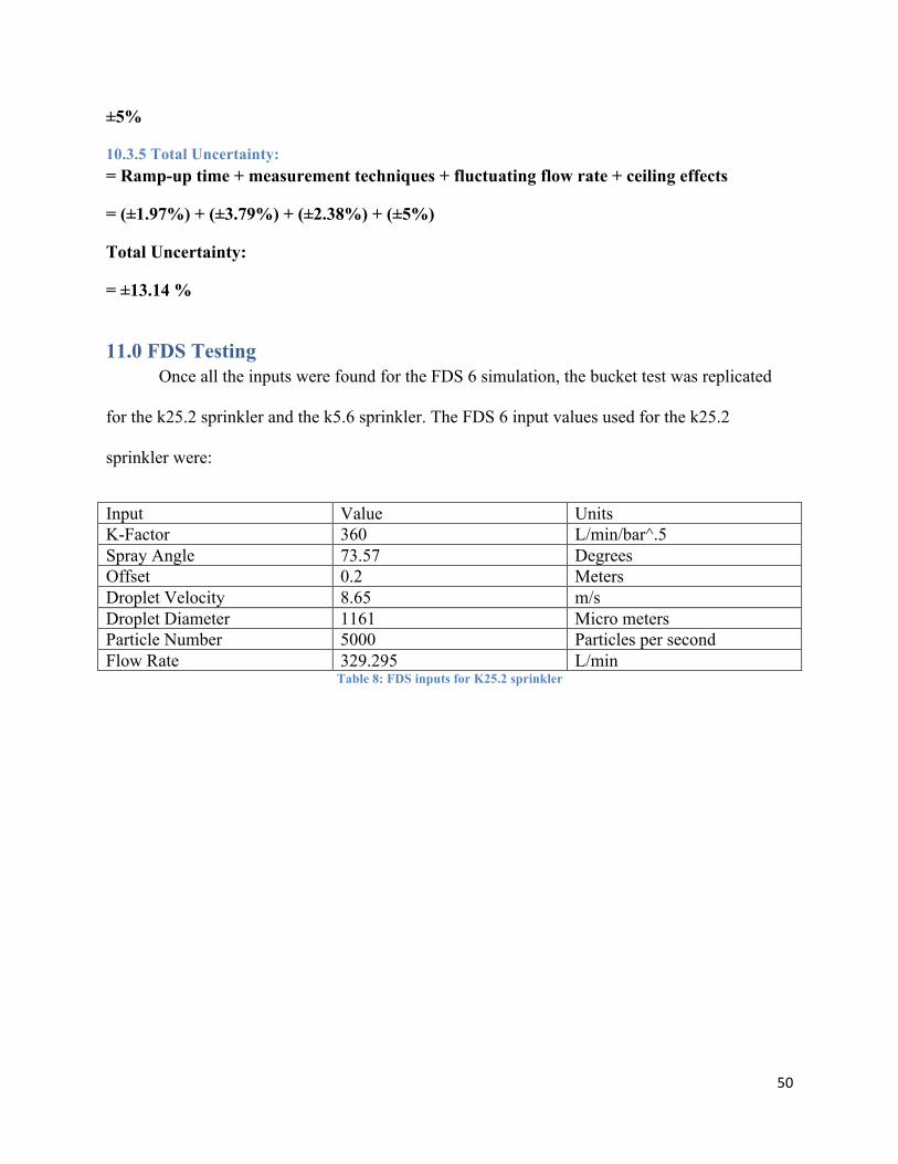
11.0 FDS Testing Once all the inputs were found for the FDS 6 simulation, the bucket test was replicated
for the k25.2 sprinkler and the k5.6 sprinkler. The FDS 6 input values used for the k25.2
sprinkler were:
Input Value Units K-Factor 360 L/min/bar^.5 Spray Angle 73.57 Degrees Offset 0.2 Meters Droplet Velocity 8.65 m/s Droplet Diameter 1161 Micro meters Particle Number 5000 Particles per second Flow Rate 329.295 L/min
Table 8: FDS inputs for K25.2 sprinkler
51
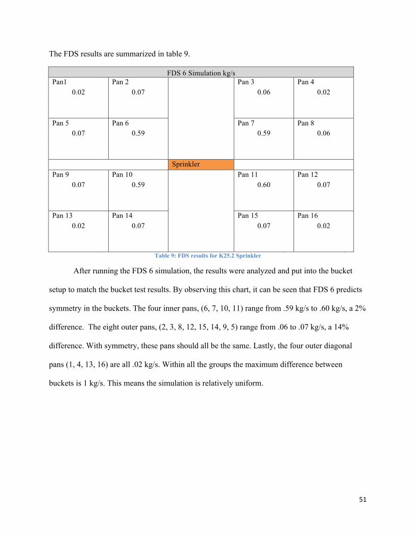
The FDS results are summarized in table 9.
FDS 6 Simulation kg/s Pan1 Pan 2 Pan 3 Pan 4
0.02 0.07 0.06 0.02 Pan 5 Pan 6 Pan 7 Pan 8
0.07 0.59 0.59 0.06 Sprinkler Pan 9 Pan 10 Pan 11 Pan 12
0.07 0.59 0.60 0.07 Pan 13 Pan 14 Pan 15 Pan 16
0.02 0.07 0.07 0.02
Table 9: FDS results for K25.2 Sprinkler
After running the FDS 6 simulation, the results were analyzed and put into the bucket
setup to match the bucket test results. By observing this chart, it can be seen that FDS 6 predicts
symmetry in the buckets. The four inner pans, (6, 7, 10, 11) range from .59 kg/s to .60 kg/s, a 2%
difference. The eight outer pans, (2, 3, 8, 12, 15, 14, 9, 5) range from .06 to .07 kg/s, a 14%
difference. With symmetry, these pans should all be the same. Lastly, the four outer diagonal
pans (1, 4, 13, 16) are all .02 kg/s. Within all the groups the maximum difference between
buckets is 1 kg/s. This means the simulation is relatively uniform.
52
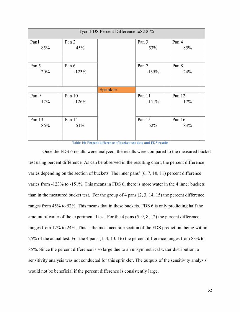
Tyco-FDS Percent Difference ±8.15 %
Pan1 Pan 2 Pan 3 Pan 4 85% 45% 53% 85%
Pan 5 Pan 6 Pan 7 Pan 8
20% -123% -135% 24% Sprinkler Pan 9 Pan 10 Pan 11 Pan 12
17% -126% -151% 17% Pan 13 Pan 14 Pan 15 Pan 16
86% 51% 52% 83%
Table 10: Percent difference of bucket test data and FDS results
Once the FDS 6 results were analyzed, the results were compared to the measured bucket
test using percent difference. As can be observed in the resulting chart, the percent difference
varies depending on the section of buckets. The inner pans’ (6, 7, 10, 11) percent difference
varies from -123% to -151%. This means in FDS 6, there is more water in the 4 inner buckets
than in the measured bucket test. For the group of 4 pans (2, 3, 14, 15) the percent difference
ranges from 45% to 52%. This means that in these buckets, FDS 6 is only predicting half the
amount of water of the experimental test. For the 4 pans (5, 9, 8, 12) the percent difference
ranges from 17% to 24%. This is the most accurate section of the FDS prediction, being within
25% of the actual test. For the 4 pans (1, 4, 13, 16) the percent difference ranges from 83% to
85%. Since the percent difference is so large due to an unsymmetrical water distribution, a
sensitivity analysis was not conducted for this sprinkler. The outputs of the sensitivity analysis
would not be beneficial if the percent difference is consistently large.
53
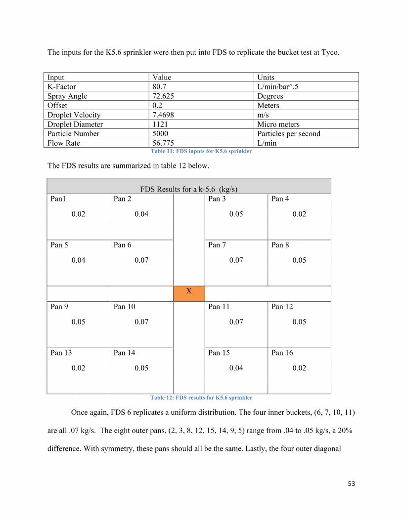
The inputs for the K5.6 sprinkler were then put into FDS to replicate the bucket test at Tyco.
Input Value Units K-Factor 80.7 L/min/bar^.5 Spray Angle 72.625 Degrees Offset 0.2 Meters Droplet Velocity 7.4698 m/s Droplet Diameter 1121 Micro meters Particle Number 5000 Particles per second Flow Rate 56.775 L/min
Table 11: FDS inputs for K5.6 sprinkler
The FDS results are summarized in table 12 below.
FDS Results for a k-5.6 (kg/s) Pan1 Pan 2 Pan 3 Pan 4
0.02 0.04 0.05 0.02
Pan 5 Pan 6 Pan 7 Pan 8
0.04 0.07 0.07 0.05
X
Pan 9
Pan 10 Pan 11 Pan 12
0.05 0.07 0.07 0.05
Pan 13 Pan 14 Pan 15 Pan 16
0.02 0.05 0.04 0.02
Table 12: FDS results for K5.6 sprinkler
Once again, FDS 6 replicates a uniform distribution. The four inner buckets, (6, 7, 10, 11)
are all .07 kg/s. The eight outer pans, (2, 3, 8, 12, 15, 14, 9, 5) range from .04 to .05 kg/s, a 20%
difference. With symmetry, these pans should all be the same. Lastly, the four outer diagonal
54
pans (1, 4, 13, 16) are all .02 kg/s. Within all the groups the maximum difference between
buckets is 1 kg/s. This means the simulation is uniform.
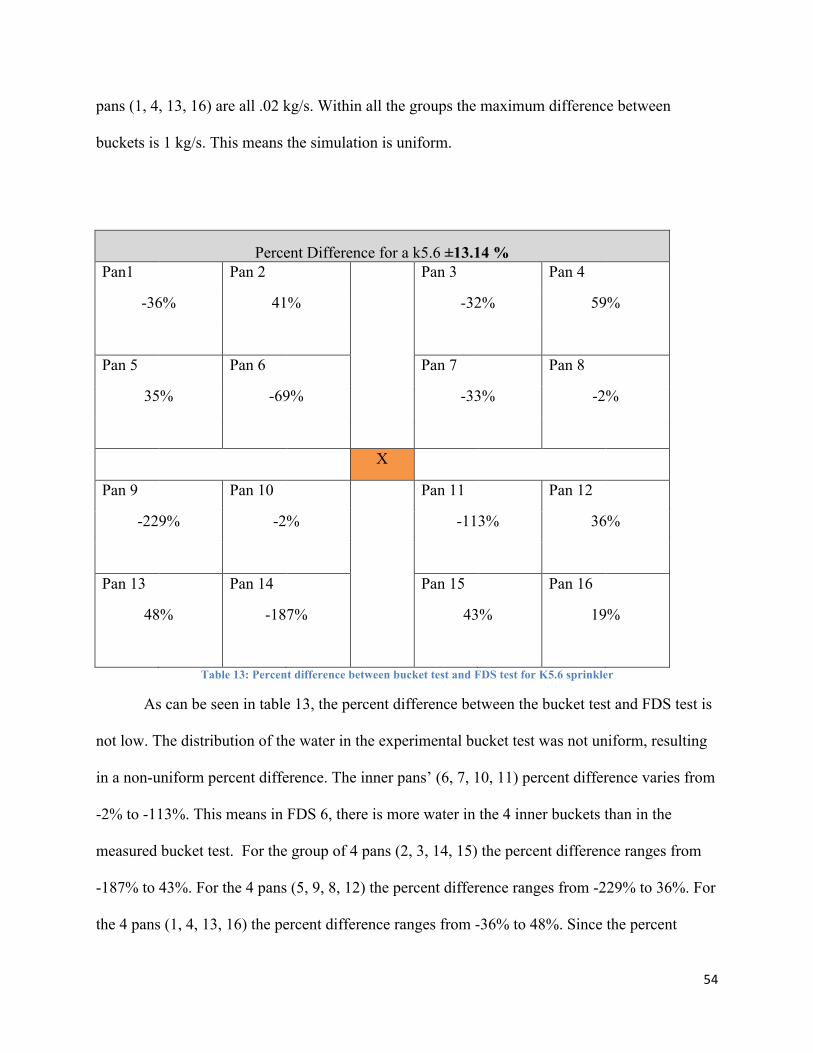
Percent Difference for a k5.6 ±13.14 % Pan1 Pan 2 Pan 3 Pan 4
-36% 41% -32% 59%
Pan 5 Pan 6 Pan 7 Pan 8
35% -69% -33% -2%
X
Pan 9
Pan 10 Pan 11 Pan 12
-229% -2% -113% 36%
Pan 13 Pan 14 Pan 15 Pan 16
48% -187% 43% 19%
Table 13: Percent difference between bucket test and FDS test for K5.6 sprinkler
As can be seen in table 13, the percent difference between the bucket test and FDS test is
not low. The distribution of the water in the experimental bucket test was not uniform, resulting
in a non-uniform percent difference. The inner pans’ (6, 7, 10, 11) percent difference varies from
-2% to -113%. This means in FDS 6, there is more water in the 4 inner buckets than in the
measured bucket test. For the group of 4 pans (2, 3, 14, 15) the percent difference ranges from
-187% to 43%. For the 4 pans (5, 9, 8, 12) the percent difference ranges from -229% to 36%. For
the 4 pans (1, 4, 13, 16) the percent difference ranges from -36% to 48%. Since the percent
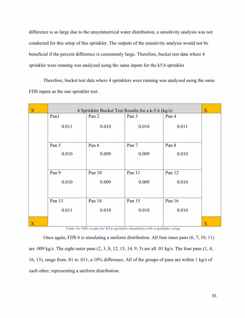
55
difference is so large due to the unsymmetrical water distribution, a sensitivity analysis was not
conducted for this setup of this sprinkler. The outputs of the sensitivity analysis would not be
beneficial if the percent difference is consistently large. Therefore, bucket test data where 4
sprinkler were running was analyzed using the same inputs for the k5.6 sprinkler
Therefore, bucket test data where 4 sprinklers were running was analyzed using the same
FDS inputs as the one sprinkler test.
X 4 Sprinkler Bucket Test Results for a k-5.6 (kg/s) X
Pan1 Pan 2 Pan 3 Pan 4
0.011 0.010 0.010 0.011
Pan 5 Pan 6 Pan 7 Pan 8
0.010 0.009 0.009 0.010
Pan 9
Pan 10 Pan 11 Pan 12
0.010 0.009 0.009 0.010
Pan 13 Pan 14 Pan 15 Pan 16
0.011 0.010 0.010 0.010
X
X Table 14: FDS results for K5.6 sprinkler simulation with 4 sprinkler setup
Once again, FDS 6 is simulating a uniform distribution. All four inner pans (6, 7, 10, 11)
are .009 kg/s. The eight outer pans (2, 3, 8, 12, 15, 14, 9, 5) are all .01 kg/s. The four pans (1, 4,
16, 13), range from .01 to .011, a 10% difference. All of the groups of pans are within 1 kg/s of
each other, representing a uniform distribution.
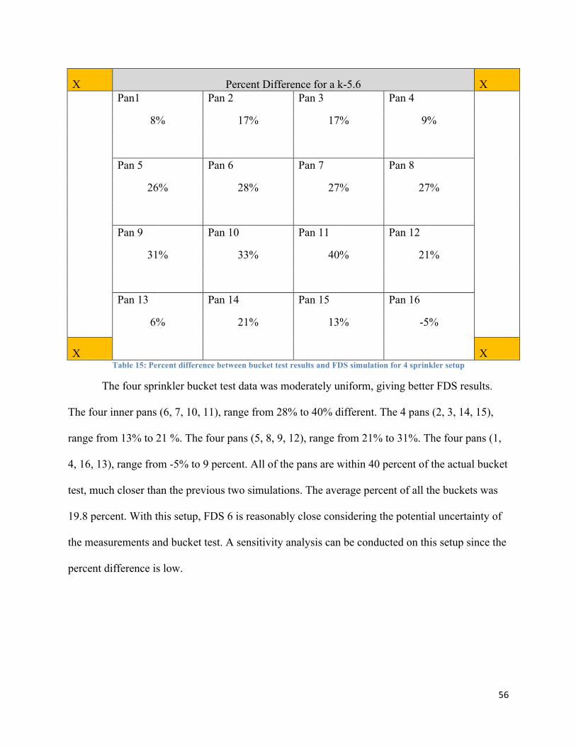
56
X Percent Difference for a k-5.6 X
Pan1 Pan 2 Pan 3 Pan 4
8% 17% 17% 9%
Pan 5 Pan 6 Pan 7 Pan 8
26% 28% 27% 27%
Pan 9
Pan 10 Pan 11 Pan 12
31% 33% 40% 21%
Pan 13 Pan 14 Pan 15 Pan 16
6% 21% 13% -5%
X
X Table 15: Percent difference between bucket test results and FDS simulation for 4 sprinkler setup
The four sprinkler bucket test data was moderately uniform, giving better FDS results.
The four inner pans (6, 7, 10, 11), range from 28% to 40% different. The 4 pans (2, 3, 14, 15),
range from 13% to 21 %. The four pans (5, 8, 9, 12), range from 21% to 31%. The four pans (1,
4, 16, 13), range from -5% to 9 percent. All of the pans are within 40 percent of the actual bucket
test, much closer than the previous two simulations. The average percent of all the buckets was
19.8 percent. With this setup, FDS 6 is reasonably close considering the potential uncertainty of
the measurements and bucket test. A sensitivity analysis can be conducted on this setup since the
percent difference is low.
57
12.0 Results of Sensitivity Analysis A sensitivity analysis was completed to determine the relative importance of each FDS
input. It was possible to discover which default values were reasonable to use and which inputs
needed to be measured for higher accuracy. The parameters included in the sensitivity analysis
were those not included in the manufacturer’s specification. These parameters were:
• Spray Offset
• Spray Angle
• Droplet Size
• Droplet Velocity
• Particles Per Second
To conduct the sensitivity analysis, deterministic and parametric approaches were used.
Deterministic analysis evaluates each parameter individually while all other parameters are held
constant [17]. Parametric analysis is moving one or a few inputs across reasonably selected
ranges, such as low to high in order to examine the shape of the response. As part of the
sensitivity analysis a base case of the best measured FDS inputs was conducted. Then using a
deterministic approach, all inputs were kept constant while changing a single input. The three
outputs for each of the sensitivity tests were average percent difference, absolute average percent
difference, and maximum absolute percent difference.
The average percent difference was calculated using a multi-step process. First, the percent
difference between the measured bucket test and the FDS simulation for all 16 buckets was
found. The percent differences for these 16 buckets were averaged to find the “average percent
difference.” This gives an indication of how well the FDS prediction was at replicating a bucket
test. In this calculation a negative percent difference would cancel out a positive, therefore not
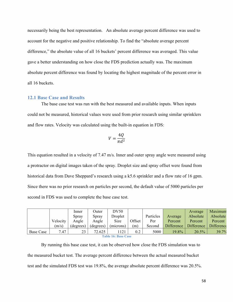
58
necessarily being the best representation. An absolute average percent difference was used to
account for the negative and positive relationship. To find the “absolute average percent
difference,” the absolute value of all 16 buckets’ percent difference was averaged. This value
gave a better understanding on how close the FDS prediction actually was. The maximum
absolute percent difference was found by locating the highest magnitude of the percent error in
all 16 buckets.
12.1 Base Case and Results The base case test was run with the best measured and available inputs. When inputs
could not be measured, historical values were used from prior research using similar sprinklers
and flow rates. Velocity was calculated using the built-in equation in FDS:
𝑉 =4𝑄𝜋𝑑!
This equation resulted in a velocity of 7.47 m/s. Inner and outer spray angle were measured using
a protractor on digital images taken of the spray. Droplet size and spray offset were found from
historical data from Dave Sheppard’s research using a k5.6 sprinkler and a flow rate of 16 gpm.
Since there was no prior research on particles per second, the default value of 5000 particles per
second in FDS was used to complete the base case test.
Velocity
(m/s)
Inner Spray Angle
(degrees)
Outer Spray Angle
(degrees)
DV50 Droplet
Size (microns)
Offset (m)
Particles Per
Second
Average Percent
Difference
Average Absolute Percent
Difference
Maximum Absolute Percent
Difference Base Case 7.47 23 72.625 1121 0.2 5000 19.8% 20.5% 39.7%
Table 16: Base Case
By running this base case test, it can be observed how close the FDS simulation was to
the measured bucket test. The average percent difference between the actual measured bucket
test and the simulated FDS test was 19.8%, the average absolute percent difference was 20.5%.
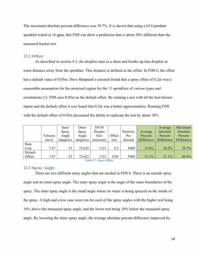
59
The maximum absolute percent difference was 39.7%. It is shown that using a k5.6 pendant
sprinkler tested at 16 gpm, that FDS can show a prediction that is about 20% different than the
measured bucket test.
12.2 Offset: As described in section 4.5, the droplets start as a sheet and breaks up into droplets at
some distance away from the sprinkler. This distance is defined as the offset. In FDS 6, the offset
has a default value of 0.05m. Dave Sheppard’s research found that a spray offset of 0.2m was a
reasonable assumption for the atomized region for the 11 sprinklers of various types and
orientations [1]. FDS uses 0.05m as the default offset. By running a test with all the best known
inputs and the default offset it was found that 0.2m was a better approximation. Running FDS
with the default offset of 0.05m decreased the ability to replicate the test by about 10%.
Velocity
(m/s)
Inner Spray Angle
(degrees)
Outer Spray Angle
(degrees)
DV50 Droplet
Size (microns)
Offset (m)
Particles Per
Second
Average Percent
Difference
Average Absolute Percent
Difference
Maximum Absolute Percent
Difference Base Case 7.47 23 72.625 1121 0.2 5000 19.8% 20.5% 39.7% Default Offset 7.47 23 72.625 1121 0.05 5000 31.1% 31.1% 46.9%
Table 17: Spray Offset
12.3 Spray Angle: There are two different spray angles that are needed in FDS 6. There is an outside spray
angle and an inner spray angle. The outer spray angle is the angle of the outer boundaries of the
spray. The inner spray angle is the small angle where no water is being sprayed on the inside of
the spray. A high and a low case were run for each of the spray angles with the higher test being
10% above the measured spray angle, and the lower test being 10% below the measured spray
angle. By lowering the inner spray angle, the average absolute percent difference improved by
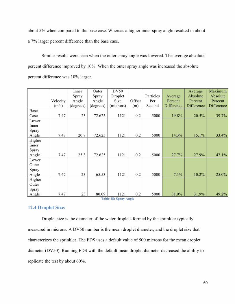
60
about 5% when compared to the base case. Whereas a higher inner spray angle resulted in about
a 7% larger percent difference than the base case.
Similar results were seen when the outer spray angle was lowered. The average absolute
percent difference improved by 10%. When the outer spray angle was increased the absolute
percent difference was 10% larger.
Velocity
(m/s)
Inner Spray Angle
(degrees)
Outer Spray Angle
(degrees)
DV50 Droplet
Size (microns)
Offset (m)
Particles Per
Second
Average Percent
Difference
Average Absolute Percent
Difference
Maximum Absolute Percent
Difference Base Case 7.47 23 72.625 1121 0.2 5000 19.8% 20.5% 39.7% Lower Inner Spray Angle 7.47 20.7 72.625 1121 0.2 5000 14.3% 15.1% 33.4% Higher Inner Spray Angle 7.47 25.3 72.625 1121 0.2 5000 27.7% 27.9% 47.1% Lower Outer Spray Angle 7.47 23 65.53 1121 0.2 5000 7.1% 10.2% 25.0% Higher Outer Spray Angle 7.47 23 80.09 1121 0.2 5000 31.9% 31.9% 49.2%
Table 18: Spray Angle
12.4 Droplet Size:
Droplet size is the diameter of the water droplets formed by the sprinkler typically
measured in microns. A DV50 number is the mean droplet diameter, and the droplet size that
characterizes the sprinkler. The FDS uses a default value of 500 microns for the mean droplet
diameter (DV50). Running FDS with the default mean droplet diameter decreased the ability to
replicate the test by about 60%.
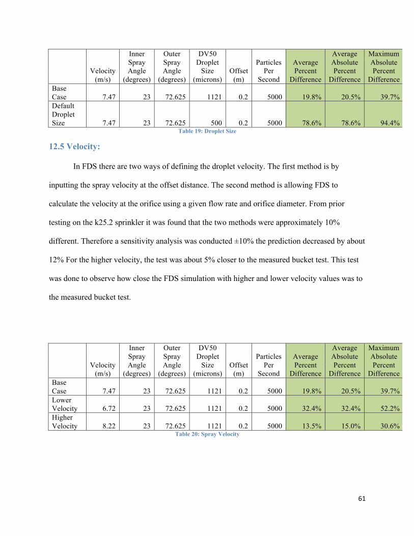
61
Velocity
(m/s)
Inner Spray Angle
(degrees)
Outer Spray Angle
(degrees)
DV50 Droplet
Size (microns)
Offset (m)
Particles Per
Second
Average Percent
Difference
Average Absolute Percent
Difference
Maximum Absolute Percent
Difference Base Case 7.47 23 72.625 1121 0.2 5000 19.8% 20.5% 39.7% Default Droplet Size 7.47 23 72.625 500 0.2 5000 78.6% 78.6% 94.4%
Table 19: Droplet Size
12.5 Velocity:
In FDS there are two ways of defining the droplet velocity. The first method is by
inputting the spray velocity at the offset distance. The second method is allowing FDS to
calculate the velocity at the orifice using a given flow rate and orifice diameter. From prior
testing on the k25.2 sprinkler it was found that the two methods were approximately 10%
different. Therefore a sensitivity analysis was conducted ±10% the prediction decreased by about
12% For the higher velocity, the test was about 5% closer to the measured bucket test. This test
was done to observe how close the FDS simulation with higher and lower velocity values was to
the measured bucket test.
Velocity
(m/s)
Inner Spray Angle
(degrees)
Outer Spray Angle
(degrees)
DV50 Droplet
Size (microns)
Offset (m)
Particles Per
Second
Average Percent
Difference
Average Absolute Percent
Difference
Maximum Absolute Percent
Difference Base Case 7.47 23 72.625 1121 0.2 5000 19.8% 20.5% 39.7% Lower Velocity 6.72 23 72.625 1121 0.2 5000 32.4% 32.4% 52.2% Higher Velocity 8.22 23 72.625 1121 0.2 5000 13.5% 15.0% 30.6%
Table 20: Spray Velocity
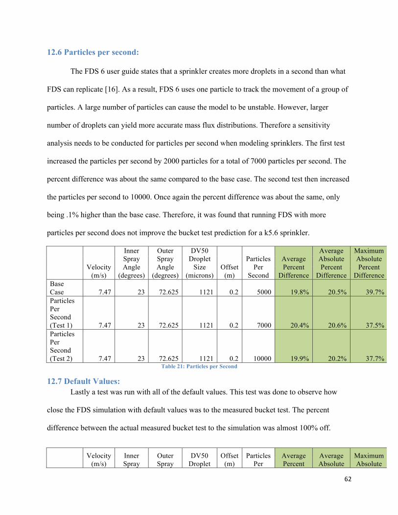
62
12.6 Particles per second:
The FDS 6 user guide states that a sprinkler creates more droplets in a second than what
FDS can replicate [16]. As a result, FDS 6 uses one particle to track the movement of a group of
particles. A large number of particles can cause the model to be unstable. However, larger
number of droplets can yield more accurate mass flux distributions. Therefore a sensitivity
analysis needs to be conducted for particles per second when modeling sprinklers. The first test
increased the particles per second by 2000 particles for a total of 7000 particles per second. The
percent difference was about the same compared to the base case. The second test then increased
the particles per second to 10000. Once again the percent difference was about the same, only
being .1% higher than the base case. Therefore, it was found that running FDS with more
particles per second does not improve the bucket test prediction for a k5.6 sprinkler.
Velocity
(m/s)
Inner Spray Angle
(degrees)
Outer Spray Angle
(degrees)
DV50 Droplet
Size (microns)
Offset (m)
Particles Per
Second
Average Percent
Difference
Average Absolute Percent
Difference
Maximum Absolute Percent
Difference Base Case 7.47 23 72.625 1121 0.2 5000 19.8% 20.5% 39.7% Particles Per Second (Test 1) 7.47 23 72.625 1121 0.2 7000 20.4% 20.6% 37.5% Particles Per Second (Test 2) 7.47 23 72.625 1121 0.2 10000 19.9% 20.2% 37.7%
Table 21: Particles per Second
12.7 Default Values: Lastly a test was run with all of the default values. This test was done to observe how
close the FDS simulation with default values was to the measured bucket test. The percent
difference between the actual measured bucket test to the simulation was almost 100% off.
Velocity
(m/s) Inner Spray
Outer Spray
DV50 Droplet
Offset (m)
Particles Per
Average Percent
Average Absolute
Maximum Absolute
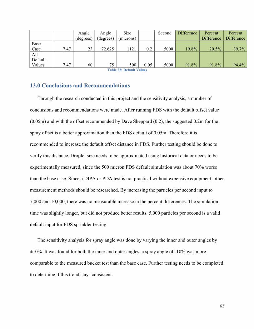
63
Angle (degrees)
Angle (degrees)
Size (microns)
Second Difference Percent Difference
Percent Difference
Base Case 7.47 23 72.625 1121 0.2 5000 19.8% 20.5% 39.7% All Default Values 7.47 60 75 500 0.05 5000 91.8% 91.8% 94.4%
Table 22: Default Values
13.0 Conclusions and Recommendations
Through the research conducted in this project and the sensitivity analysis, a number of
conclusions and recommendations were made. After running FDS with the default offset value
(0.05m) and with the offset recommended by Dave Sheppard (0.2), the suggested 0.2m for the
spray offset is a better approximation than the FDS default of 0.05m. Therefore it is
recommended to increase the default offset distance in FDS. Further testing should be done to
verify this distance. Droplet size needs to be approximated using historical data or needs to be
experimentally measured, since the 500 micron FDS default simulation was about 70% worse
than the base case. Since a DIPA or PDA test is not practical without expensive equipment, other
measurement methods should be researched. By increasing the particles per second input to
7,000 and 10,000, there was no measurable increase in the percent differences. The simulation
time was slightly longer, but did not produce better results. 5,000 particles per second is a valid
default input for FDS sprinkler testing.
The sensitivity analysis for spray angle was done by varying the inner and outer angles by
±10%. It was found for both the inner and outer angles, a spray angle of -10% was more
comparable to the measured bucket test than the base case. Further testing needs to be completed
to determine if this trend stays consistent.
64
As stated previously, in FDS there are two ways of defining the droplet velocity. The first
method is by inputting the spray velocity at the offset distance. The second method is allowing
FDS to calculate the velocity at the orifice using a given flow rate and orifice diameter. When the
droplet velocity was increased, a closer prediction was observed. However, from section 4.2 it
was found that for most droplet sizes, the maximum droplet velocity is at the orifice due to air
resistance. Further testing of other sprinkler types is recommended to see if a higher velocity
than the one at the orifice continues to produce a closer FDS prediction.
65
References [1] Sheppard, D., ‘‘Spray Characteristics of Fire Sprinklers,’’ PhD Thesis, Northwestern University, 2002 (see also NIST GCR 02-838).
[2] Schwille, J.A. & Lueptow, R.M., A simplified model of the effect of a fire sprinkler spray on a buoyant fire plume. Journal of Fire Protection Engineering, 2006; 16:131-153. [3] Mahmud, H., Moinudin, K., Thorpe,G., “Characterization of Water-mist Spray: Numerical Modeling and Experimental Validation,” Victoria University, 2012. [4] Mahmood, T., Dubiel, D., Troolin, D., Hart, P., “Complex Spray Pattern Measurements for Fire Sprinkler Modeling,” Underwriters Laboratories, Northbrook, Ill, 2011. [6] Marshall, A. W. and diMarzo, M., “Modeling Aspects of Sprinkler Spray Dynamics in Fires (Review),” Process Safety and Environmental Protection, Transaction of the Institution of Chemical Engineers: Part B, Vol. 82, pp. 97-104, 2004. Particle Image Velocimetry : A Practical Guide, 2nd ed. Raffel, Markus. Springer, 2007. [7] Comeau, D., LaTourette, K., Pate, J., “The Effect of Weber Number and Spread Factor of a Water Droplet Impinging on a Super-Hydrophobic Substrate,” University of Arizona. December 2007 [8] Ren, N., Blum, A., Zheng, Y. H., Do, C., and Marshall, A. W., "Quantifying the Initial Spray from Fire Sprinklers, " Fire Safety Science – Proceedings of the Ninth International Symposium, IAFSS, Karlsruhe, Deutschland, Accepted, 2008. [9] Particle Image Velocimetry : New Developments and Recent Applications (3-540-73527-5, 978-3-540-73527-4), Schroeder, Andreas. Springer, 2008. [10] PIV (Particle Image Velocimetry) Principle. University of Minnesota. http://www.aem.umn.edu/people/students/troolin/tutorial_piv_principle.html [11] Particle Image Velocimetry : A Practical Guide, 2nd ed. Raffel, Markus. Springer, 2007. [12] Putorti, A. D., “Simultaneous Measurements of Drop Size and Velocity in Large-Scale Sprinkler Flows Using Particle Tracking and Laser-Induced Fluorescence.” National Institute of Standards and Technology, NIST GCR 04-861, February 2004 [13] T.S. Chan. Measurements of Water Density and Droplet Size Distributions of Selected ESFR Sprinklers. Journal of Fire Protection Engineering, 6(2):79–87, 1994. [14] Widmann, J. F.; Sheppard, D. T.; Lueptow, R. M., “Non-Intrusive Measurements in Fire Sprinkler Sprays”, Fire Technology, Vol. 37, No. 4, 297-315, 4th Quarter, October 2001. [15] Floyd, J., Forney, G., Hostikka, S., Kornhonen, T., Macdermott, W., & McGrattan, K., Fire Dynamics Simulator (Version 6), Technical Reference Guide, Volume 1: Mathematical Model,
66
NIST Special Publication 1018, National Institute of Standards and Technology (NIST), U.S. Department of Commerce, Gaithersburg, Maryland, USA, 2012. [16] Floyd, J., Forney, G., Hostikka, S., Kornhonen, T., Macdermott, W., & McGrattan, K., Fire Dynamics Simulator (Version 6), User’s Guide, NIST Special Publication 1019, National Institute of Standards and Technology (NIST), U.S. Department of Commerce, Gaithersburg, Maryland, USA, 2012. [17] Morgan, M., & Henrion, M., “Uncertainty”, Cambridge University Press, New York, NY, 1990.
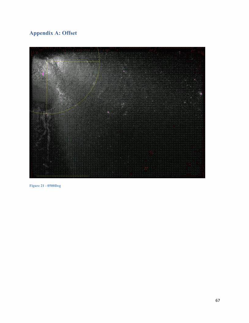
67
Appendix A: Offset
Figure 21 - 0500Deg
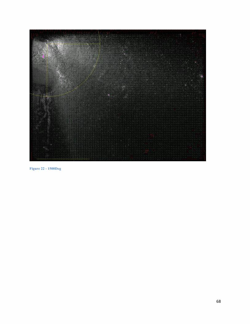
68
Figure 22 - 1500Deg
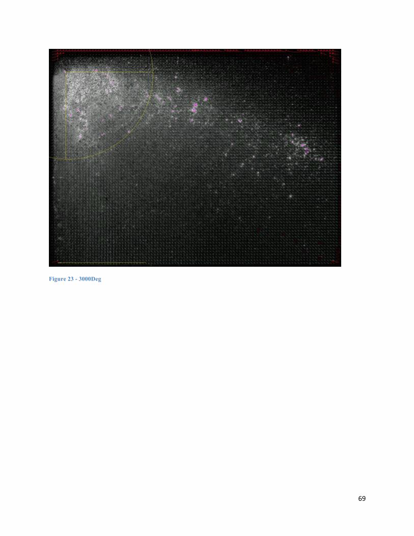
69
Figure 23 - 3000Deg
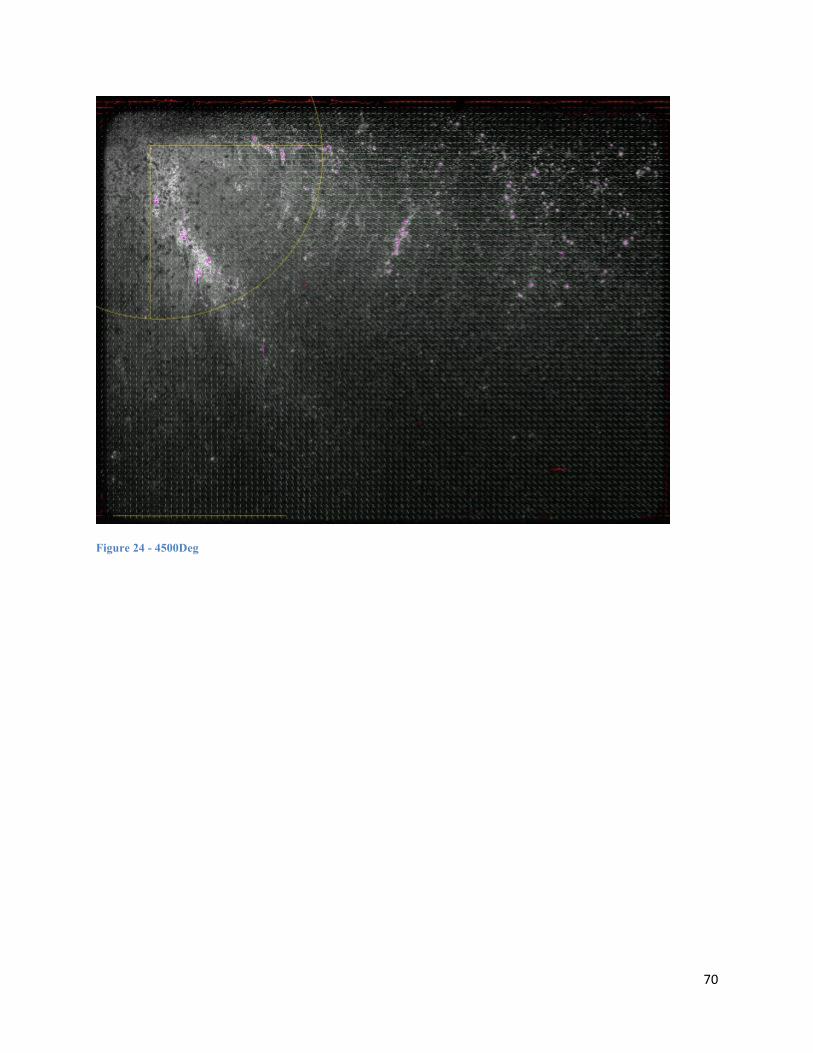
70
Figure 24 - 4500Deg
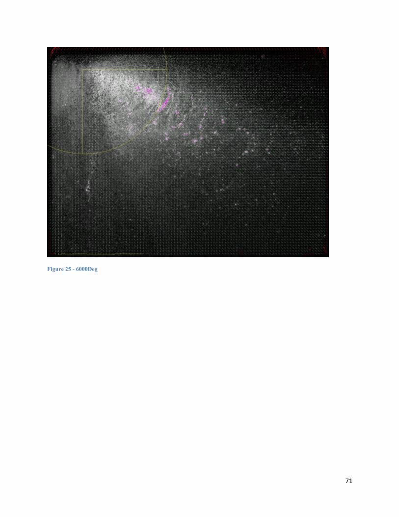
71
Figure 25 - 6000Deg
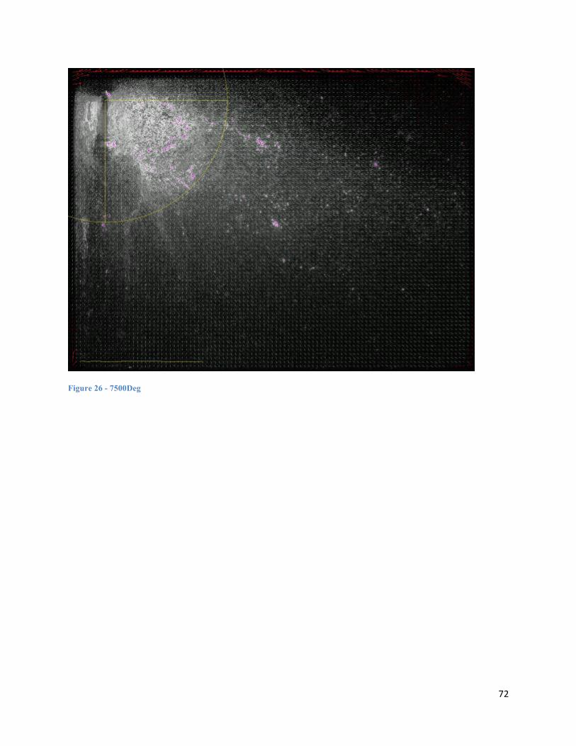
72
Figure 26 - 7500Deg
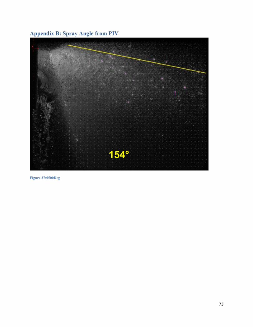
73
Appendix B: Spray Angle from PIV
Figure 27:0500Deg
154°
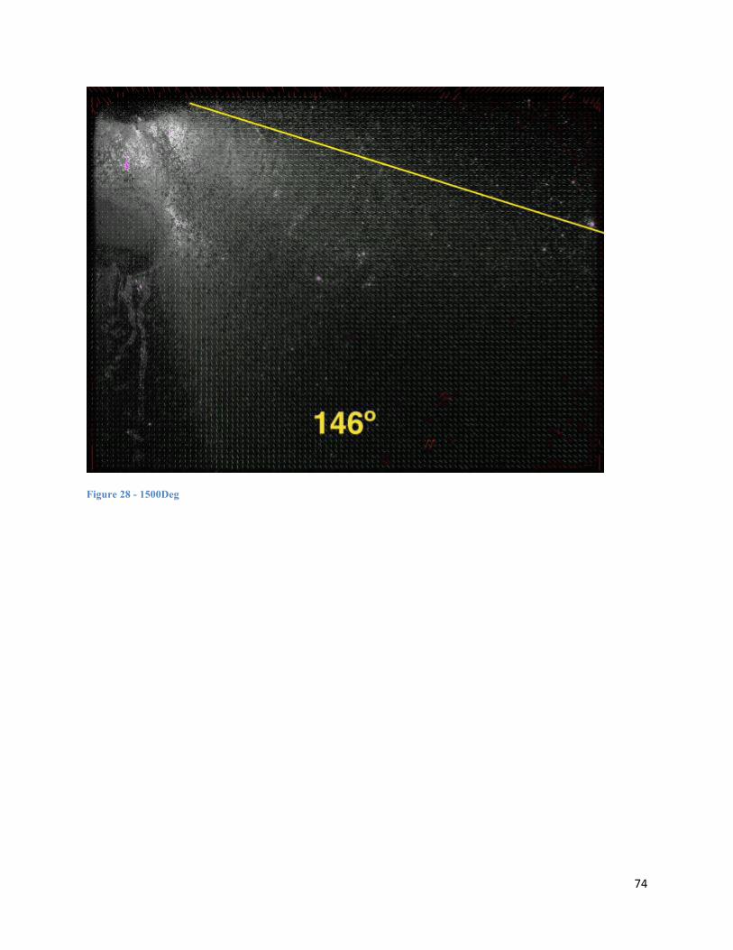
74
Figure 28 - 1500Deg
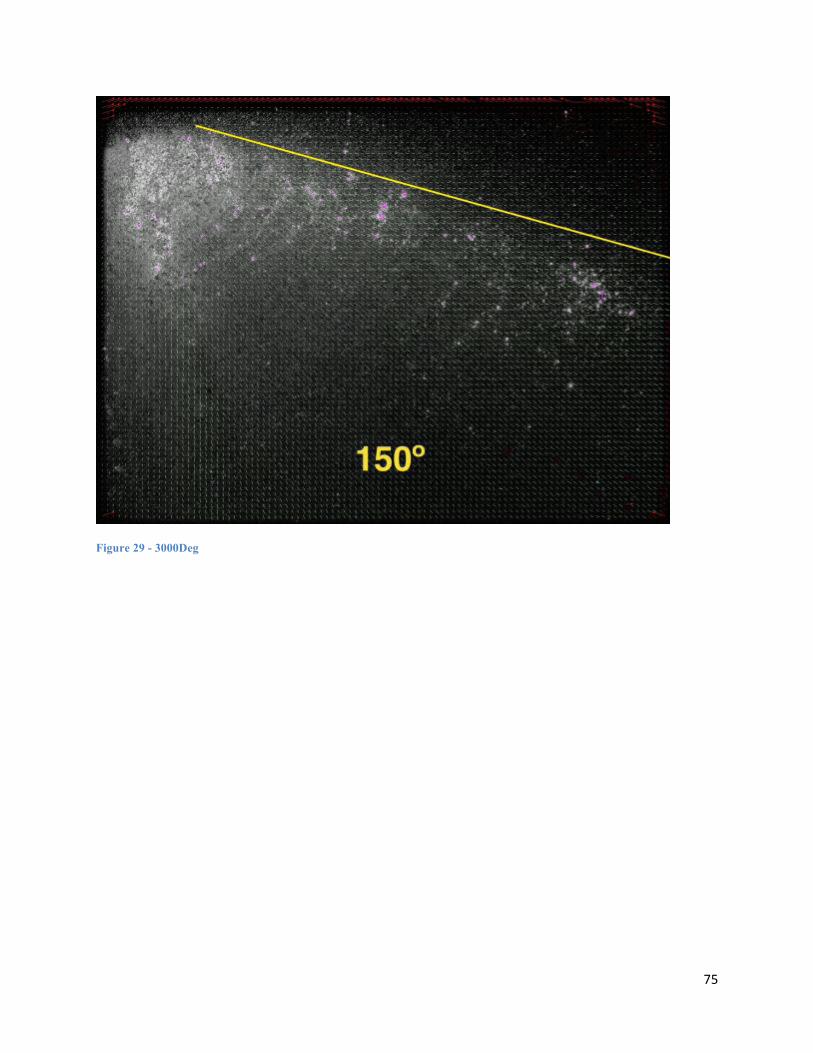
75
Figure 29 - 3000Deg
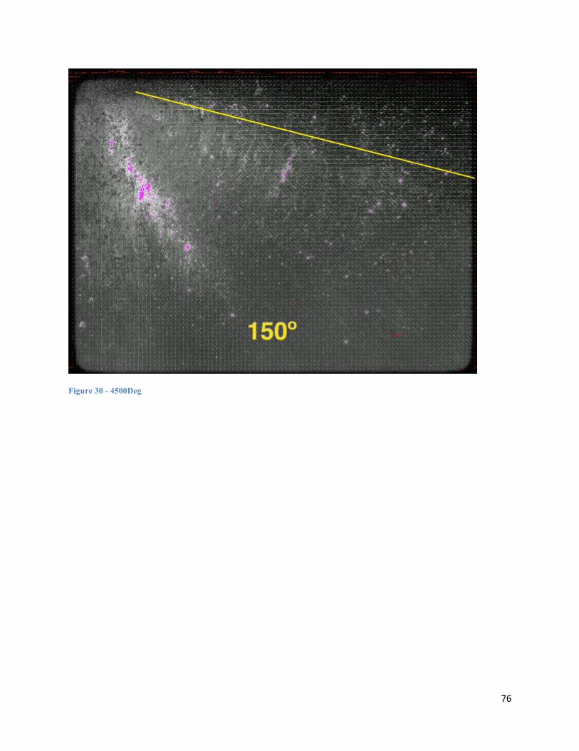
76
Figure 30 - 4500Deg
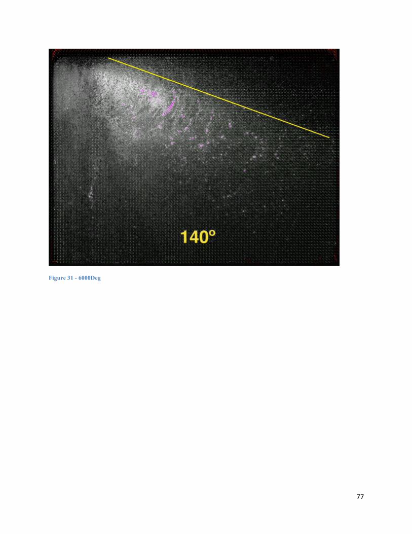
77
Figure 31 - 6000Deg
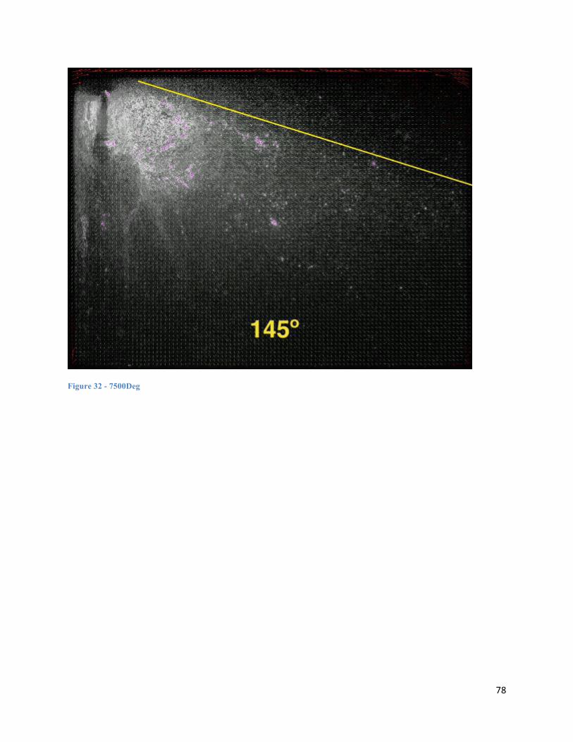
78
Figure 32 - 7500Deg
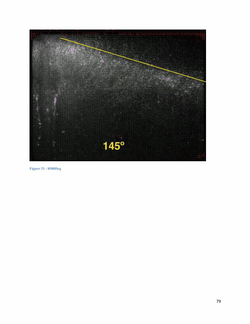
79
Figure 33 - 8500Deg
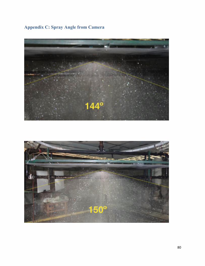
80
Appendix C: Spray Angle from Camera
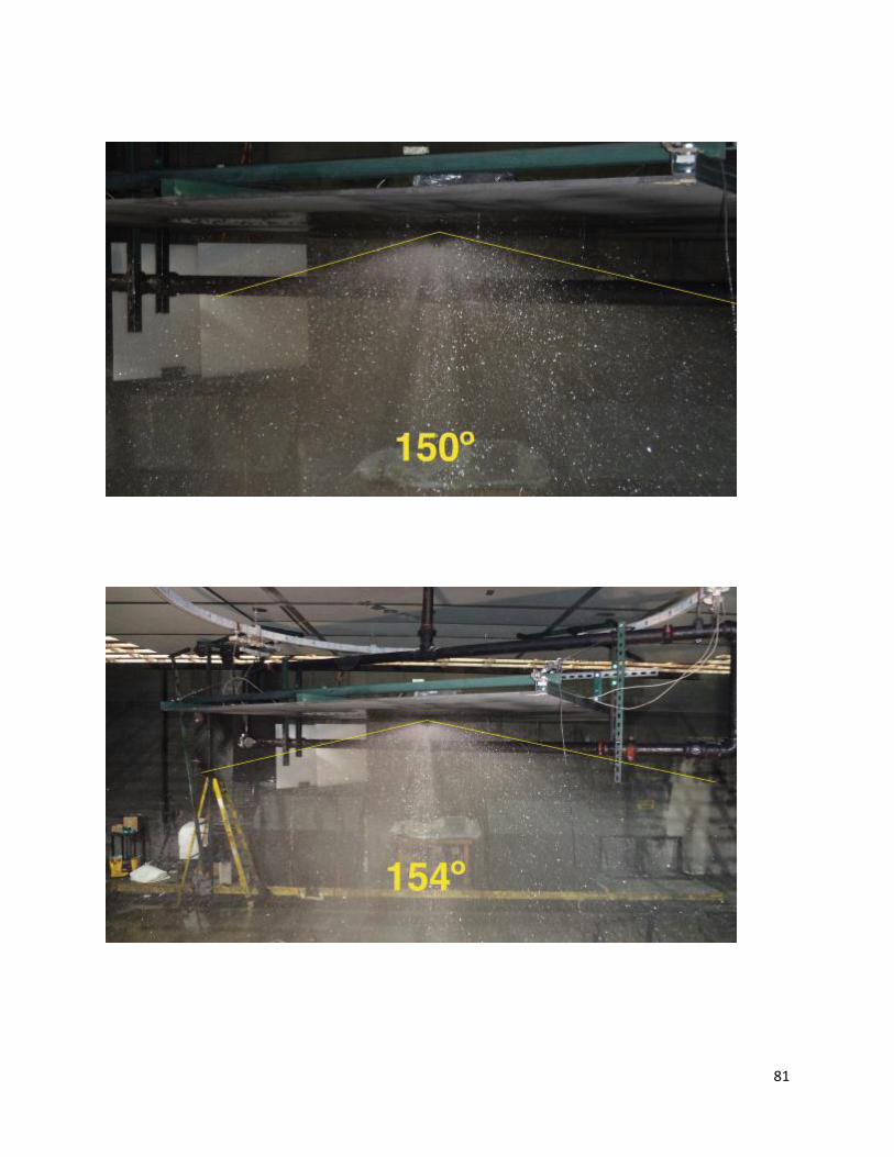
81
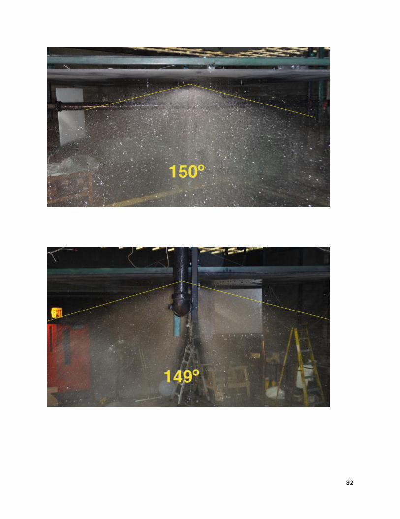
82
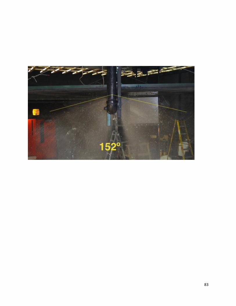
83
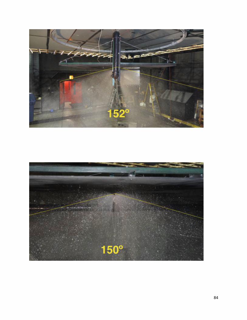
84
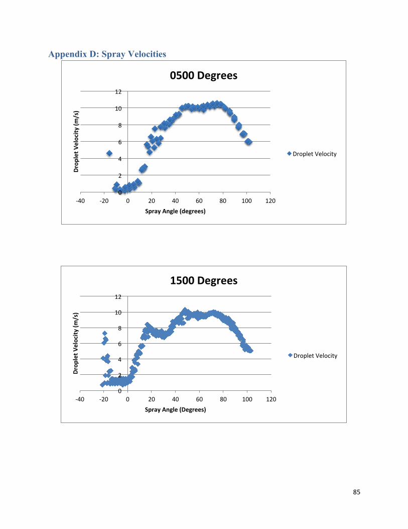
85
Appendix D: Spray Velocities
0
2
4
6
8
10
12
-‐40 -‐20 0 20 40 60 80 100 120
Drop
let V
elocity
(m/s)
Spray Angle (degrees)
0500 Degrees
Droplet Velocity
0
2
4
6
8
10
12
-‐40 -‐20 0 20 40 60 80 100 120
Drop
let V
elocity
(m/s)
Spray Angle (Degrees)
1500 Degrees
Droplet Velocity
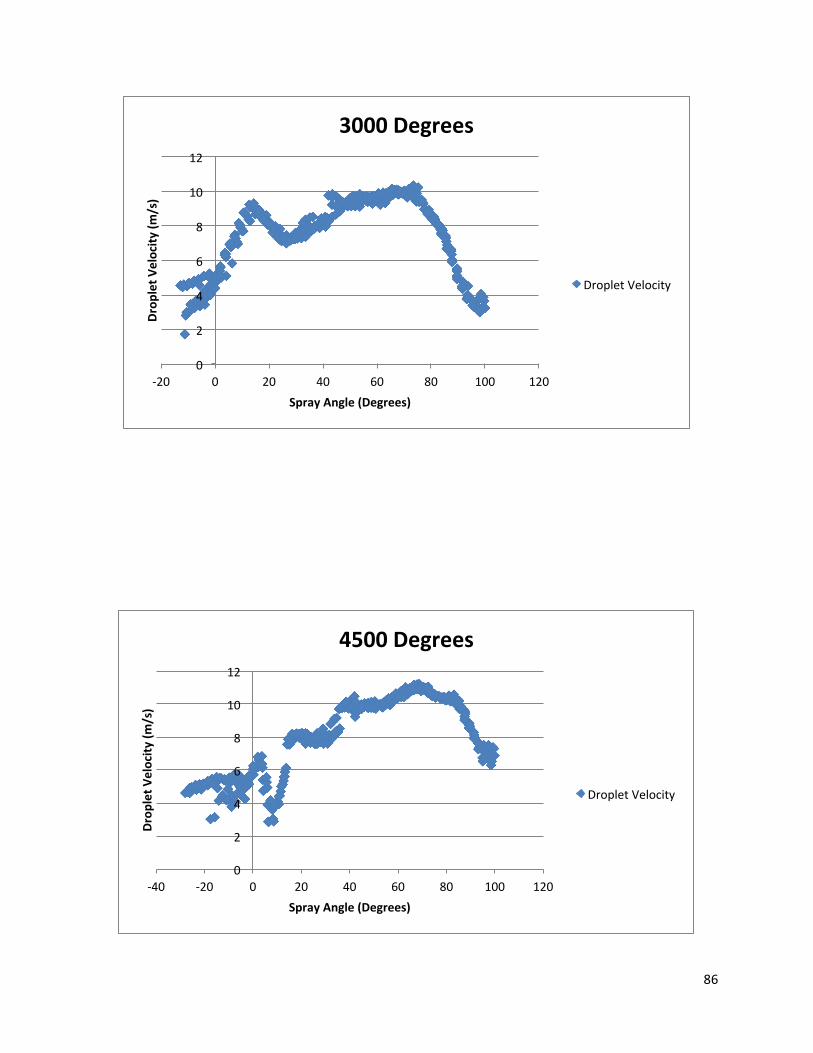
86
0
2
4
6
8
10
12
-‐20 0 20 40 60 80 100 120
Drop
let V
elocity
(m/s)
Spray Angle (Degrees)
3000 Degrees
Droplet Velocity
0
2
4
6
8
10
12
-‐40 -‐20 0 20 40 60 80 100 120
Drop
let V
elocity
(m/s)
Spray Angle (Degrees)
4500 Degrees
Droplet Velocity
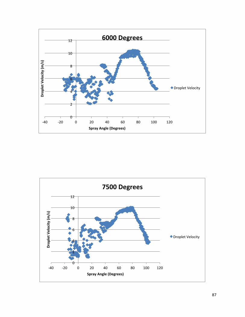
87
0
2
4
6
8
10
12
-‐40 -‐20 0 20 40 60 80 100 120
Drop
let V
elocity
(m/s)
Spray Angle (Degrees)
6000 Degrees
Droplet Velocity
0
2
4
6
8
10
12
-‐40 -‐20 0 20 40 60 80 100 120
Drop
let V
elocity
(m/s)
Spray Angle (Degrees)
7500 Degrees
Droplet Velocity
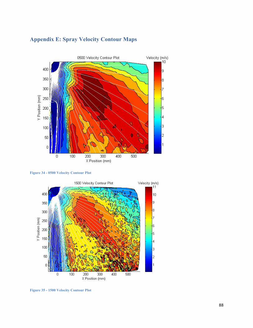
88
Appendix E: Spray Velocity Contour Maps
Figure 34 - 0500 Velocity Contour Plot
Figure 35 - 1500 Velocity Contour Plot
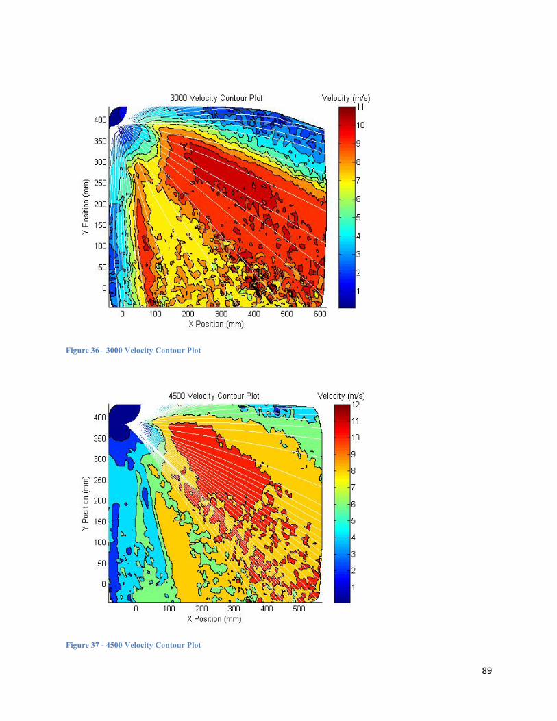
89
Figure 36 - 3000 Velocity Contour Plot
Figure 37 - 4500 Velocity Contour Plot
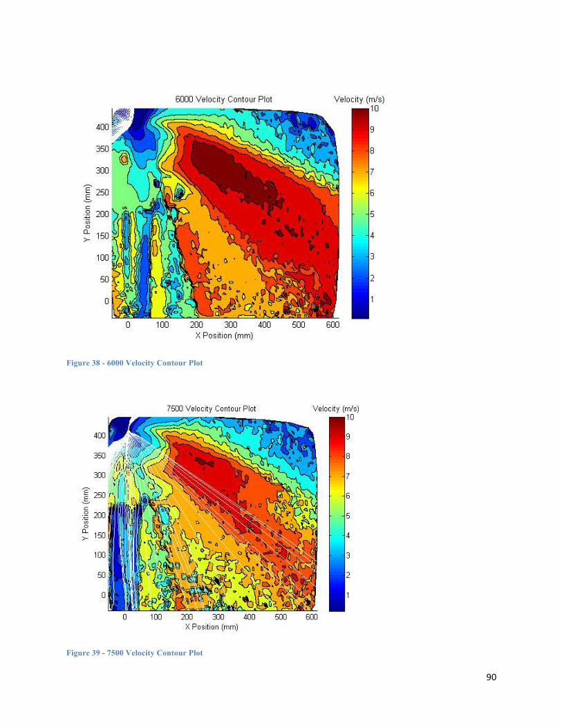
90
Figure 38 - 6000 Velocity Contour Plot
Figure 39 - 7500 Velocity Contour Plot
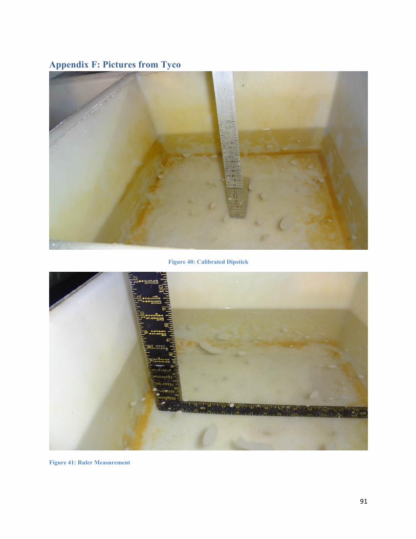
91
Appendix F: Pictures from Tyco
Figure 40: Calibrated Dipstick
Figure 41: Ruler Measurement
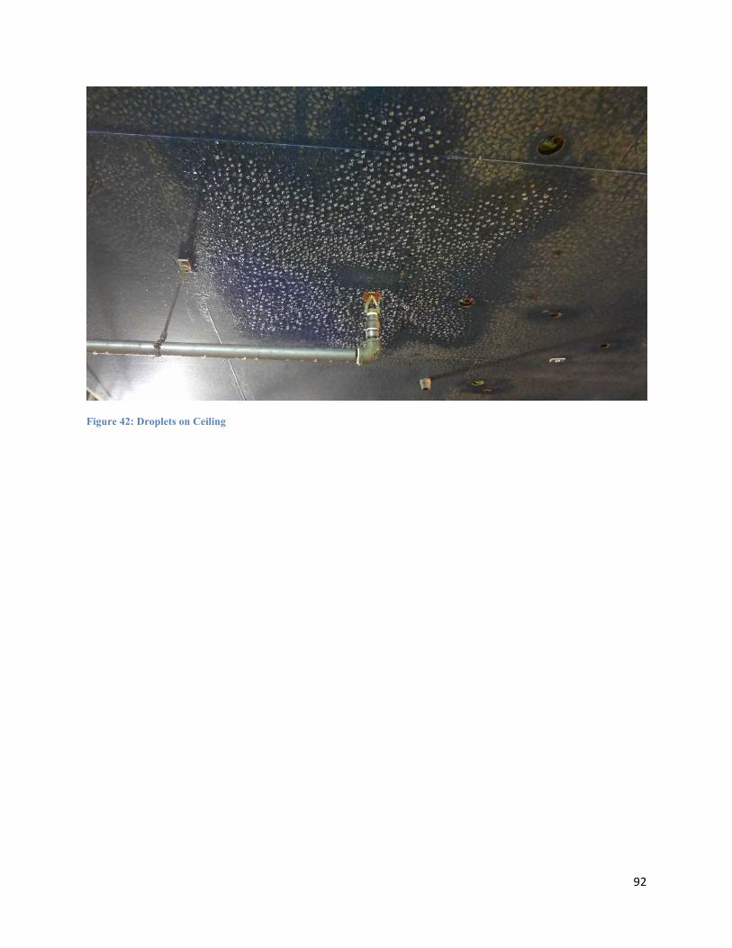
92
Figure 42: Droplets on Ceiling
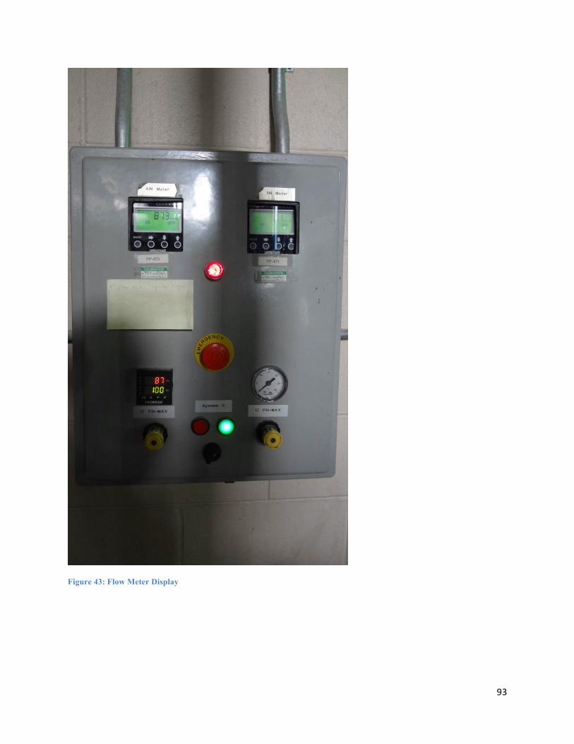
93
Figure 43: Flow Meter Display