1

7C-1 6th Asia-Oceania Symposium on Fire Science and Technology 17-20, March, 2004, Daegu, Korea

Numerical Simulation of a Compartment Fire in Activation of a Sprinkler

Futoshi TANAKA1, Yoshifumi OHMIYA1, and Yoshihiko HAYASHI2

1Tokyo University of Science, 2641 Yamasaki Noda-shi CHIBA-KEN 278-8510, JAPAN 2Building Research Institute, 1 Tatehara Tukuba-shi IBARAKI-KEN 305-0802, JAPAN

Abstract

The purpose of this study is the establishment of the Computational Fluid Dynamics (CFD) field model, taking into consideration water discharge equipments, such as sprinkler equipments (SP). The fire control effect of the water discharge equipment was investigated using a CFD field model. The computational results were compared with a full-scale compartment fire experiment in which the water discharge equipment was installed. When the water discharge equipment was not used, the computational results of the temperature distribution in the compartment were in agreement with the experimental results. When the water discharge equipment was used, the numerical simulation could not predict the experimental value with sufficient accuracy. One of the causes for decrease in prediction accuracy is the condensation heat transfer mechanism generated on the wet wall. In this study, the prediction accuracy of the numerical simulation could improve by taking into consideration the condensation heat transfer.

1. Introduction*

The Building Standards Law (BSL) of Japan was revised in June 1999 to partly include the idea of functional requirements. At present, fire prevention requirements in BSL have introduced functional as well as conventional specification requirements. The Fire Safety Performance required of buildings was stipulated by the functional requirements in the fire resistance requirements. However, the effect Corresponding Author- Tel.: +81-4-7124-1501;

Fax: +81-4-7122-9744 E-mail address: f-tanaka@rs.noda.tus.ac.jp

of water discharge equipments, such as sprinkler equipments (SP) and water mist equipments (WM), is not fully taken into consideration in the fire prevention requirements. In forming the fire safety design of buildings, the evaluation of fire external force is important. The fire external force is reduced by the fire suppression effect of water discharge equipments. Therefore, a design with high flexibility is attained. However, engineering knowledge of fire extinguishment and the control by water discharge equipments is not enough. Subsequently, we performed a full-scale compartment fire experiment [1, 2]. In this experiment, the heat release rate of the fire source,

Copyright © International Association for Fire Safety Science

2

the temperature distributions in a compartment, heat flux, and other parameters were measured. The quantitative knowledge of fire suppression effect by using water discharge equipment was obtained from this full-scale compartment fire experiment. However, the experiment cases conducted are still few in number. It is necessary to systematically change the parameters related to fire behavior and perform substantial comparison and examination. For example, the experimental parameters including the compartment scale and form, the amount of combustibles and their positions, the position of water discharge heads and the amount of water discharge, and so on. However, conducting a full-scale experiment for such a parametric study, is time consuming and very expensive. This study aimed at the establishment of the Computational Fluid Dynamics (CFD) field model as an analysis tool, to complement the full-scale experiments. The fire control effect of water discharge equipments using a CFD field model was investigated [3].

2. Outline of the full-scale fire experiments

2.1 The experimental facility

The experimental facility used for the full-

scale fire experiments is shown in Fig.1. The experimental facility is a compartment (W5.0m × B5.0m × H2.41m) prepared as a fire room. This facility was installed in the fire extinguishing research building of the National Research Institute of Fire and Disaster (NRIFD). The heat source (combus tibles) was installed in the center of the compartment. The installed position of SP is shown in Fig. 2. One set of SP was installed on the ceiling directly above the fire source. The operating pressure of SP was 0.1 MPa and its volume flux was 80 L/min.

2. 2 Setup for measurements and heat source

A sheathed thermocouple (0.64 mm) was

used for the measurement of temperature. Within the compartment, the temperature distributions in the perpendicular direction were measured at the following four locations: the heat source C1, the near right corner C2 and the far left corner C3, from the opening, and the opening C4. The measurement positions are shown in Fig.1. Heat fluxes were measured using three water-cooled heat flux meters. The first meter was located on the ceiling directly above the heat source, the second meter was located at the center of the north wall, and the final meter was located in the heat source. The heat flux meter located in the heat source was installed with the measurement face facing the ceiling. This heat flux meter measured feedback heat flux from the flame to the heat source. The gas, which passed through the compartment opening, was collected in the hood. The heat release rate of the heat source was measured using the oxygen consumption method. N-heptane and a wooden crib were used as combustibles for the heat source. Two kinds of experimental conditions are compared using the CFD field model. The first experiment condition is the free combustion condition, which is conducted in the compartment. In this condition, pool fires burning 2 L of n-heptane were used as the heat source. The second condition is the fire control condition by operating SP. Both these conditions use the same heat source. The time histories of the heat release rate measured in the experiments are shown in Fig.3 by solid lines. In the case where SP is not used (free), the heat release rate shows a peak value, which leads to the belief that this fire behavior is of fuel-controlled fire. In the cases where SP is used (SP), it is found that the heat release rate is controlled by SP. Although the heat release rate is controlled, the fire could not be extinguished. Therefore,

3

combustibles (2 L of n-heptane) burned slowly for a long time.

C3

900 1, 2501,

250

1,25

01, 250 2, 500

2,50

0

6, 274

6,27

4

C2

C4

C1

Heat sour ce

Fig.1 Schematic representation of an experimental compartment (unit: mm)

900

Openi ng

5, 0002, 500

2,50

0

5,00

0 SP

Fig.2 Installation position of SP (unit: mm)

Time (sec)

H.R

.R. (

kW)

SP Active29s

SP

Free

0 100 200 300 400 500

100

200

300

Fig.3 Heat release rate

3. Numerical method

In this study, the Fire Dynamics

Simulator (FDS), developed by McGrattan et al. at the National Institute of Standards and Technology (NIST), was used as a computational code [4]. Here, we briefly summarize the CFD models (turbulence, combustion, radiation, etc.) used in the FDS [5]. 3.1 Governing equations

The governing equations used in the FDS consist of the conservation equations of mass, momentum, energy, chemical species, and a state equation.

0=⋅∇+∂∂ uρρ

t (1)

( ) ( ) τfguuu

⋅∇++−=∇+⎟⎠⎞

⎜⎝⎛ ∇⋅+∂∂

∞ρρρ pt

(2)

( )

∑ ∇⋅∇+∇⋅∇+⋅∇−

=⋅∇+∂∂

llllr YDhTk

DtDp

hht

ρ

ρρ

q

u (3)

lllll mYDY

tY

+∇⋅∇=⋅∇+∂∂ ρρρ u (4)

( )∑= ii MYTRp /0 ρ (5)

3.2 Temporal and spatial discretization

The explicit predictor-corrector method is used as the time integral method. As regards the time step, the suitable value is set up using the local Courant-Friedrichs-Lewy (CFL) condition. In this study, the average time step was about 0.5 seconds. The second order central difference is used as spatial discretization. The convective terms are written as upwind-biased differences in the predictor step and downwind-biased differences in the corrector step. The local CFL number is used as the bias of upwind differences and downwind differences [6].

N

x

y

x

y

4

3.3 Turbulence and combustion model A Large Eddy Simulation (LES) using a

standard Smagorinsky model as a Sub-Grid Scale (SGS) model is performed in the FDS. Thermal and chemical species diffusion improves by the mixed effect of small eddies in the turbulence flow field. In an LES, the thermal conductivity and the chemical species diffusivity are related to the turbulent viscosity by

PrpLES

LES

Ck

μ= (6)

( )Sc

D LESLESl

μρ =, (7)

where Pr is the Prandtl number and Sc is

the Schmidt number. In this numerical simulation, the Smagorinsky constant was at a constant value of 0.2, and Pr and Sc were assumed at a constant value of 0.5. A mixture fraction model is used as a combustion model. The mixture fraction model adopted here assumes that fuel and oxygen burn instantaneously when mixed. This is a good assumption for large-scale, well-ventilated fires. In the mixture fraction model used by the FDS, a flame surface is defined as a surface where fuel and oxygen vanish simultaneously. It is assumed that heat release by combustion is generated only on a flame surface

3.4 Thermal radiation model

The Radiative Transport Equation (RTE) for a non-scattering gas is

[ ]),()(),(),( sxxxsxs III b −=∇⋅ λκλ (8) where λI is the radiation intensity at wave length λ , s is the direction vector of the intensity, and κ is the local absorption coefficient. In practical numerical simulations, the radiation spectrum is divided into a small number of important bands, and a separate RTE is derived for each band. In this study, the gas was dealt with as gray gas when SP was not used. In

the case, when SP was used, the gaseous radiation spectrum was divided in six bands in order to take the spectrum of water vapor into consideration. The source term bI is defined as

zoneflameInsidezoneflameOutside

4//4

⎩⎨⎧

=πβπκσ

κqT

Ib & (9)

here, q& is the chemical heat release rate per unit volume and β is the local fraction of the energy emitted as thermal radiation. The value of the local fraction β was determined as 0.35 in comparison with a pool fire experiment [7]. 3.5 Sprinkler model

When SP is operated, the water droplets are emitted from the water discharge equipment, and the numerical simulation is performed. Influence of the water droplets on the flow field is taken into consideration as the body force term of the momentum conservation equation (2).

( )V

rCd ddd∑ −−=

uuuuf

2

21 πρ (10)

Here, Cd is the drag coefficient, rd is the

droplet radius, ud is the velocity of the droplets, u is the velocity of air, ρ is the density of the air, and V is the volume of the grid cell. The trajectory of the water droplets is governed by the following equation of motion.

( ) ( ) uuuugu −−−=∂∂

dddddd rCdmmt

2

21 πρ (11)

Furthermore, the evaporation of the

droplets and the radiation scattering by the droplets is also taken into consideration in the numerical simulation.

5

4. Outline of the numerical simulations

4.1 Computational domain and grid cells

The computational grid used for numerical simulation is shown in Fig. 4. In the experimental facility, the hood was prepared in the upper part, outside the compartment. However, in the numerical simulation, the hood was omitted for reducing the computational costs. The computational domain (5m(x) × 5m(y) × 2.41m(z)) was made only in the compartment used as a fire room. The dimensions of the computational grid were 36(x) × 36(y) × 48(z). The non-uniform computational grid, which was collected near the fire source, was used. The numerical simulation, which increased the dimensions of the computational grids to 48(x) × 48(y) × 64(z), was also performed. The qualitative tendency of the computational result did not change. Moreover, the change in the quantitative value was also slight.

Fig.4 Computational grid

4.2 Initial and boundary conditions, and the heat release rate

A little fluctuation was applied using a random number as the initial condition of velocity. The measurement value of the ambient air temperature in each experiment was used as the initial condition of the numerical simulations. Since the computational grid was not fine enough to resolve the boundary layer, the boundary condition of the velocity on a wall was set to be a fraction of the velocity (0.75) in the grid cell adjacent to the wall. As the

boundary condition of temperature, as shown in an equation (12), the heat flux qc, was set using the empirical heat transfer coefficient hw. As shown in an equation (13), the heat transfer coefficient hw, was calculated using the empirical equation of a forced convection and a natural convection. A larger value was chosen as the heat transfer coefficient. Since the Reynolds number, Re, is proportional to the characteristic length, L, the heat transfer coefficient is weakly related to L. for this reason, L is taken to be 1m for simulations.

Thq wc Δ= (12)

⎥⎦

⎤⎢⎣

⎡ Δ= 3/15/43/1 PrRe037.0,maxLkTChw (13)

The operating pressure and flow rate of

SP were set up similar to the experiment. The average diameter of the droplets was set to 1.0 mm. SP operated it automatically in those experiments where it was used. The activation time of SP was 29 seconds after lighting the heat source. In the numerical simulation, SP was forced to operate after 29 seconds under the same conditions. The heat release rate, measured in the full-scale experiment, was set as the heat source and numerical simulation was performed.

5. Results and discussion

The moving average, which used 15

points, was applied to the time history data obtained from the numerical simulation. 5.1 Free combustion in the compartment

A comparison of the temperature distribution in the compartment, in case of conducting free combustion, is shown in Fig.5. In the temperature distribution of the thermocouple tree C2 and C3, the calculated results and the experimental results were consistent with each other. The numerical simulation results have demonstrated that the air layer stratifies into two layers. Changes in the temperature distribution in

Heat source

x y

z

6

C4 did not coincide with the experimental results. The influence of the outlet boundary condition and the numerical diffusion are considered to be the cause. Four minutes after lighting the heat source, the temperature distribution of the thermocouple tree C1, installed directly above the heat source, showed a different tendency from the experimental result. The visualization of the flame surface 239.6 seconds after lighting the heat source is shown in Fig.6 (a). Moreover, Fig.6 (b) is the visualization of the flame surface after 326.2 seconds. These figures show that the flame surface, which grew from the heat source has almost

reached the ceiling. The thermocouple tree C1 was covered in the flame surface. It has recently been established that the calculation accuracy of the mixture fraction combustion model, used in the FDS, decreases near the flame surface [8]. Therefore, it is believed that the different tendency from the experimental results was acquired at the thermocouple tree C1. The calculation and the experimental results of the temperature at a height of 0.9 m are not in agreement due to the same reason. At this height, the flame surface is always near the thermocouple C1.

Temperature (DegC)

Hei

ght (

m)

CFD 0minCFD 2minCFD 4minCFD 6minCFD 8min

EXP 0minEXP 2minEXP 4minEXP 6minEXP 8min

C1

0 200 400 600 8000

0.5

1

1.5

2

Temperature (DegC)

Hei

ght (

m) EXP 0min

EXP 2minEXP 4minEXP 6minEXP 8minCFD 0minCFD 2minCFD 4minCFD 6minCFD 8min

C2

0 50 100 150 2000

0.5

1

1.5

2

(a) C1 (b) C2

EXP 0minEXP 2minEXP 4minEXP 6minEXP 8minCFD 0minCFD 2minCFD 4minCFD 6minCFD 8min

Temperature (DegC)

Hei

ght (

m) C3

0 50 100 150 2000

0.5

1

1.5

2

Temperature (DegC)

Hei

ght (

m) EXP 0min

EXP 2minEXP 4minEXP 6minEXP 8minCFD 0minCFD 2minCFD 4minCFD 6minCFD 8min

C4

0 50 100 150 2000

0.5

1

1.5

2

(c) C3 (d) C4

Fig. 5 Temperature distributions during free combustion

7

(a) 239.6 sec (b) 326.2 sec

Fig. 6 Visualization of the flame surface

Time (sec)

Hea

t Flu

x (k

W/m

2 ) CFD CeilingCFD WallCFD Source

EXP CeilingEXP WallEXP Source

Source

Wall

Ceiling

0 100 200 300 400 500 6000.1

1

10

100

1000

Fig. 7 Heat flux during free combustion

The time histories of heat flux obtained

from the experiment and the numerical simulation are shown in Fig. 7. The heat fluxes were obtained from: the ceiling above the heat source, the center of the north wall, and the heat source. The experimental results and the calculation results obtained from the heat flux meter on the center of the north wall coincide with each other. The calculation value of the heat flux on a ceiling peaks at 250 seconds and 290 seconds, and a different tendency from the experimental value is seen. This cause is also considered since the flame surface can reach the ceiling. The value of the heat flux on the heat source is mostly decided by the radiation from the flame surface, which encloses the surroundings. The calculation result of the heat flux on the heat source corresponds

with the experimental result. This calculation value is influenced by the local fraction, β , included in the radiative source term. As regards the local fraction, β = 0.35 was used in this study. Since the calculation result corresponds to the experimental result well, it is believed that this value is suitable. 5.2 Controlled combustion in the compartment

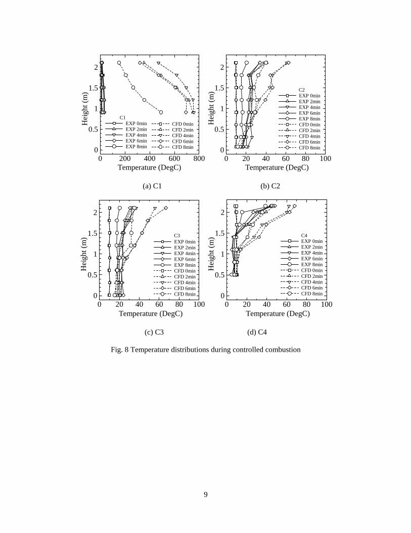
Fig. 8 shows the temperature distributions in case where SP is used. The tendency of the calculation value and the experimental value is qualitatively in agreement. However, in the numerical simulation, the temperature close to the ceiling was predicted twice as high as that of

Thermocouple

OpeningFlame surface

Fire source

8

the experiment. When SP is used, a large amount of water vapor is generated because the water droplets emitted by SP evaporate. The water vapor is then condensed on the surface of a wall, and it forms water film. This process is known as filmwise condensation heat transfer. This process is industrially applied in heat pipes, etc. It is found that the heat transfer significantly improves in the case of such a condensation heat transfer mechanism. It is necessary to take this condensation heat transfer mechanism into consideration in the numerical simulation. In this paper, the condensation heat transfer coefficient condh was dealt with as follows.

wcond hh α= (14) The heat transfer coefficient of mist cooling was made reference, and the correction coefficientα was set to 10 [9].

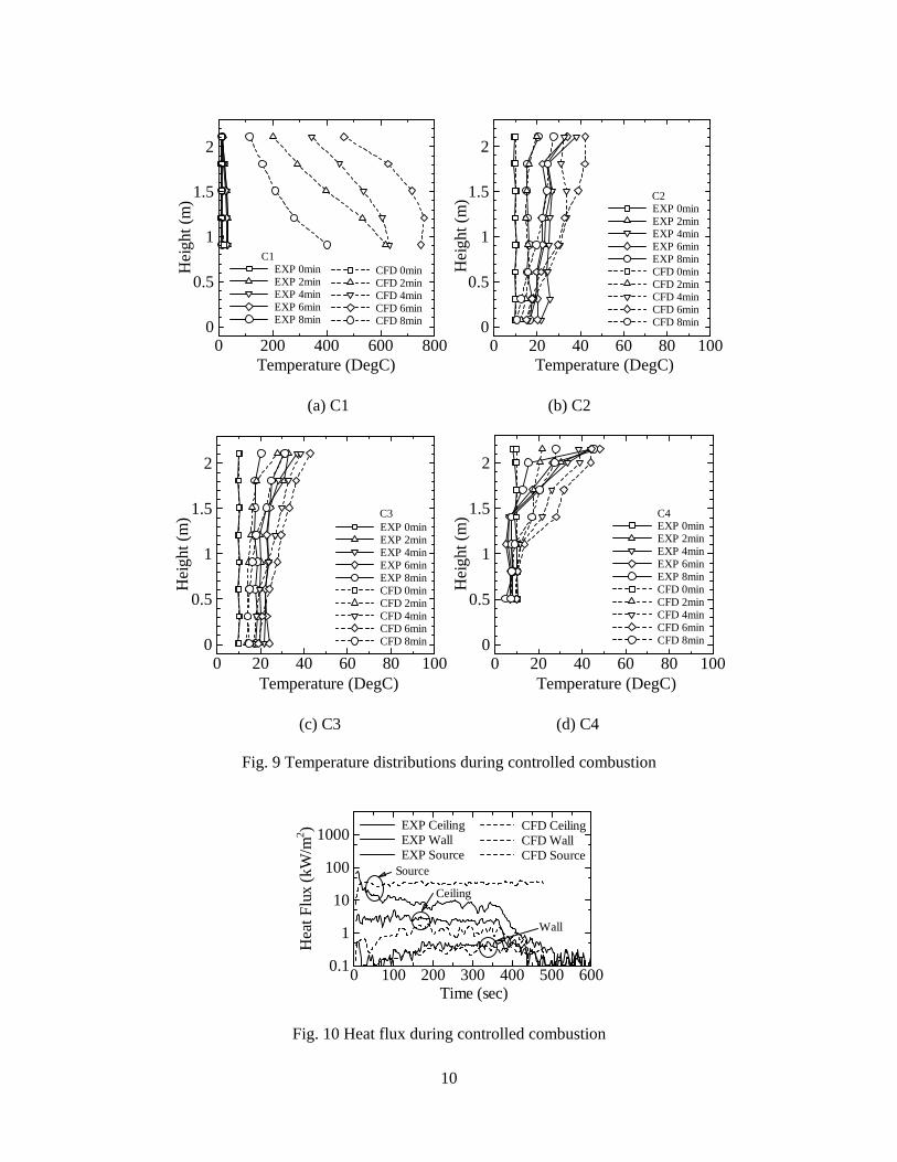
The temperature distributions in this case are shown in Fig.9. In Fig.9 (b), (c), and (d), the tendency of the numerical simulation corresponds with that of experiment. When SP is used, the prediction accuracy is improved by taking into consideration the condensation heat transfer model. The thermocouple tree C1 (Fig.9 (a)) is directly exposed to many droplets from SP. Consequently, the temperature of the water droplets is measured as a temperature distribution. Therefore, the calculation value cannot be compared with the experimental value.

A comparison of the time history of the heat flux obtained from the experiment and the numerical simulation is shown in Fig. 10. The heat flux obtained from the numerical

simulation on the heat source showed a somewhat larger tendency compared with that of the experiment. The calculation value of the heat flux for the ceiling was underestimated compared with the experimental value. The heat flux of the north wall corresponds with that of the experiments. The radiative heat flux, which reached the ceiling and the north wall, was influenced by the scattering effect of the droplets emitted by SP. The scattering effect of the radiation was dealt with using the Mie scattering theory in FDS. Further examination of a radiation scattering model may be necessary.

6. Conclusion

A numerical simulation was performed

for the purpose of prediction for a compartment fire with an opening, using Computational Fluid Dynamics. When sprinkler equipment (SP) was not used, the numerical simulation was able to successfully predict the experiment. When SP is used, the numerical simulation could not predict the experimental value with sufficient accuracy. The condensation heat transfer on the wet wall is considered to be one of the causes for the decrease in prediction accuracy. In this study, the prediction accuracy of the numerical simulation was improved by taking into consideration the condensation heat transfer. It is necessary to perform the modeling of the condensation heat transfer mechanism as a future subject.

9

Temperature (DegC)

Hei

ght (

m)

CFD 0minCFD 2minCFD 4minCFD 6minCFD 8min

EXP 0minEXP 2minEXP 4minEXP 6minEXP 8min

C1

0 200 400 600 8000

0.5

1

1.5

2

Temperature (DegC)

Hei

ght (

m) EXP 0min

EXP 2minEXP 4minEXP 6minEXP 8minCFD 0minCFD 2minCFD 4minCFD 6minCFD 8min

C2

0 20 40 60 80 1000

0.5

1

1.5

2

(a) C1 (b) C2

EXP 0minEXP 2minEXP 4minEXP 6minEXP 8minCFD 0minCFD 2minCFD 4minCFD 6minCFD 8min

Temperature (DegC)

Hei

ght (

m) C3

0 20 40 60 80 1000

0.5

1

1.5

2

Temperature (DegC)

Hei

ght (

m) EXP 0min

EXP 2minEXP 4minEXP 6minEXP 8minCFD 0minCFD 2minCFD 4minCFD 6minCFD 8min

C4

0 20 40 60 80 1000

0.5

1

1.5

2

(c) C3 (d) C4

Fig. 8 Temperature distributions during controlled combustion

10

Temperature (DegC)

Hei

ght (

m)

CFD 0minCFD 2minCFD 4minCFD 6minCFD 8min

EXP 0minEXP 2minEXP 4minEXP 6minEXP 8min

C1

0 200 400 600 8000

0.5

1

1.5

2

Temperature (DegC)

Hei

ght (

m) EXP 0min

EXP 2minEXP 4minEXP 6minEXP 8minCFD 0minCFD 2minCFD 4minCFD 6minCFD 8min

C2

0 20 40 60 80 1000

0.5

1

1.5

2

(a) C1 (b) C2

EXP 0minEXP 2minEXP 4minEXP 6minEXP 8minCFD 0minCFD 2minCFD 4minCFD 6minCFD 8min

Temperature (DegC)

Hei

ght (

m) C3

0 20 40 60 80 1000

0.5

1

1.5

2

Temperature (DegC)

Hei

ght (

m) EXP 0min

EXP 2minEXP 4minEXP 6minEXP 8minCFD 0minCFD 2minCFD 4minCFD 6minCFD 8min

C4

0 20 40 60 80 1000

0.5

1

1.5

2

(c) C3 (d) C4

Fig. 9 Temperature distributions during controlled combustion

Time (sec)

Hea

t Flu

x (k

W/m

2 ) CFD CeilingCFD WallCFD Source

EXP CeilingEXP WallEXP Source

Source

Wall

Ceiling

0 100 200 300 400 500 6000.1

1

10

100

1000

Fig. 10 Heat flux during controlled combustion

11

Acknowledgements

The authors would like to thank Dr. N.

Saito and Dr. T. Tsuruda who belong to the National Research Institute of Fire and Disaster (NRIFD).

References

1. Y. Ohmiya et al., Compartment Fire

Controlled by Fire Preventive and Suppression System, Summaries of Technical Papers of Annual Meeting, Architectural Institute of Japan A-2, pp.219-202, 2002.8 (in Japanese)

2. Y. Ohmiya et al., A Study on Control of Compartment Fire Part 1, Outline of Study, Spring Meeting, Japan Association of Fire Safety Engineering, pp.4-7, 2002.5 (in Japanese)

3. F. Tanaka et al., Numerical Analysis of Compartment Fire in case of using Sprinkler System, Summaries of Technical Papers of Annual Meeting, Architectural Institute of Japan A-2, pp.13-14, 2003.9 (in Japanese)

4. URL http://fire.nist.gov/fds/ 5. McGrattan, K. et al., Fire Dynamics

Simulator (Version3)-Technical Reference Guide, NISTIR6783, 2002

6. Continillo, G. et al., Seventh International Conference on Numerical Combustion, p.99, 1998

7. Mell, W. E. et al., Second International Conference on Fire Research and Engineering (ICFRE), pp.26-36, 1997.8

8. T.G. Ma, J. G. Quintiere, Numerical simulation of axi-symmetric fire plumes: accuracy and limitations, Fire Safety Journal 38, pp.467-492, 2003

9. Wu-Shung Fu, Toshio Aihara, Trans. Jpn. Soc. Mech. Eng., 51-463B, pp.882-891, 1985 (in Japanese)

Nomenclature

C: natural convection coefficient (-) Cd: drag coefficient (-) Cp: specific heat (J/kgK) Cs: Smagorinsky constant (-) D: diffusion coefficient (m2/s) f: external force vector (N/m3) g: acceleration of gravity (m/s2) h: enthalpy (J/kg) hcond: condensation heat transfer coefficient (W/m2K) hv: heat of vaporization (J/kg) hw: heat transfer coefficient (W/m2K) I: radiation intensity (W/m2str) k: thermal conductivity (W/mK) M: molecular weight (-) md: mass of a droplet (kg) ml: production rate of lth species per unit volume (kg/m3s) Pr: Prandtl number (-) P: pressure (Pa) q̇: heat release rate per unit volume (W/m3) qr: radiative heat flux vector (W/m2) R: universal gas constant (J/kgK) Re: Reynolds number (-)

12

rd: water droplet radius (m) s: unit vector in direction of radiation intensity (-) Sc: Schmidt number (-) T: temperature (K) t: time (s) u: velocity vector (m/s) V: computational cell volume (m3) X: volume fraction (-) Y: mass fraction (-) α : corrective coefficient (-) β : local fraction (-) κ : absorption coefficient (m-1) ρ : density (kg/m3) σ : Stefan-Boltzmann constant (W/m2K4) τ : viscous stress tensor (N/m2)