Embed Size (px)
Citation preview
Computational Homogenization of Piezoelectric Materialsusing FE2 Methods and Configurational Forces
Dem Fachbereich Maschinenbau und Verfahrenstechnik
der Technischen Universität Kaiserslautern
zur Erlangung des akademischen Grades
Doktor-Ingenieur (Dr.-Ing.)
genehmigte Dissertation
von
Herrn
M.Sc. Md Khalaquzzaman
aus Dinajpur, Bangladesch
Hauptreferent: Prof. Dr.-Ing. Ralf MüllerKorreferent: Prof. Dr. Bai-Xiang XuVorsitzender: Prof. Dr.-Ing. Eberhard KerscherDekan: Prof. Dr.-Ing. Christian Schindler
Tag der Einreichung: 29.10.2014Tag der mündlichen Prüfung: 15.04.2015
Kaiserslautern, 2015
D 386
Herausgeber
Lehrstuhl für Technische MechanikTechnische Universität KaiserslauternGottlieb-Daimler-StraßePostfach 304967653 Kaiserslautern
© Md Khalaquzzaman
Ich danke der „Prof. Dr. Hans Georg und Liselotte Hahn Stiftung” für die finanzielle Un-terstützung bei der Drucklegung.
Druck
Technische Universität KaiserslauternZTB - Abteilung Foto-Repro-Druck
Alle Rechte vorbehalten, auch das des auszugsweisen Nachdrucks, der auszugsweisenoder vollständigen Wiedergabe (Photographie, Mikroskopie), der Speicherung in Daten-verarbeitungsanlagen und das der Übersetzung.
ISBN 978-3-942695-10-7

Acknowledgement
First of all, I am highly grateful to my supervisor Prof. Dr.-Ing. Ralf Müller for his contin-ual mentoring and support throughout this dissertation. I thank him for the guidance andadvice which brought my dissertation to success. I would like to thank the co-supervisorProf. Dr. Bai-Xiang Xu for her effort to review this work. My special thanks goes toProf. Dr.-Ing. Eberhard Kerscher for chairing the examination committee.
I would like to thank Dr.-Ing. Sarah Staub for her valuable discussions on computationalhomogenization. I specially thank Dr.-Ing. David Schrade, M.Sc. Matthias Sabel for theirhelp to my dissertation in various ways. I am thankful to all of my colleagues from theInstitute of Applied Mechanics for their support. I want to express my gratefulness to theBangladeshi community in Kaiserslautern for their mental and social support throughoutthe time of my dissertation.
I want to thank my wife and my family for their support and encouragement.
Finally, I acknowledge the financial support of German Research Foundation (DFG) in theframework of the Graduate Program GRK 814 at TU Kaiserslautern. I also acknowledgethe financial support of the Center for Mathematical and Computational Modeling (CM)2
of TU Kaiserslautern.
Md Khalaquzzaman26/07/2015, Kaiserslautern
3

Zusammenfassung
Piezoelektrische Materialien besitzen die Eigenschaft, elektrische und mechanische Sig-nale zu koppeln. Bei diesen Werkstoffen ist es möglich, durch Aufbringen einer mech-anischen Last, ein elektrisches Feld zu erzeugen. Dieses Phänomen bezeichnet man alsden piezoelektrischen Effekt. Umgekehrt führt das Anlegen einer elektrischen Spannungzu einer mechanischen Deformation, was als inverser piezoelektrischer Effekt bezeich-net wird. Aufgrund dieser Eigenschaften von piezoelektrischen Materialien, werden siehäufig in Sensoren und Aktoren eingesetzt. Ferroelektrische oder piezoelektrische Materi-alien ändern ihre Polarisation durch Aufbringen äußerer Lasten. Dank dieser Eigenschaft,können sie als dauerhafter Speicher mit direktem Zugriff eingesetzt werden. Um dieseWerkstoffe in technischen Anwendungen effektiv einzusetzen, ist eine genaue Beschrei-bung des Antwortverhaltens erforderlich. Aufgrund des wachsenden Bedarfs nach einerexakten Charakterisierung, gewinnen numerische Methoden zunehmend an Bedeutung.
Viele Konstruktionswerkstoffe besitzen Inhomogenitäten auf mikroskopischer Ebene. Di-ese Inhomogenitäten erschweren die Charakterisierung des Antwortverhaltens mit exper-imentellen sowie numerischen Methoden. Andererseits können diese Defekte auch posi-tive Eigenschaften hervorrufen; so weisen faserverstärkte Kunststoffe eine hohe Festigkeitauf, bei gleichzeitig niedrigem Gewicht. Auch bei piezoelektrischen Materialien spielenInhomogenitäten auf der Mikroebene eine wichtige Rolle. Diese Inhomogenitäten resul-tieren zum einen aus der Struktur der Werkstoffe, die aus Domänen und Domänenwände,Körnern und Korngrenzen, sowie mikroskopischen Rissen besteht. Um den Einfluss derMikrostruktur auf das Verhalten der Makrostruktur zu berücksichtigen, muss eine Ho-mogenisierung der physikalischen Eigenschaften (z.B. in Form von Materialparametern)erfolgen. Eine Möglichkeit dazu ist die klassische Zwei-Skalen-Homogenisierung ersterOrdnung mittels der FE2-Methode, die in dieser Arbeit behandelt wird. Das Ziel dieserArbeit ist es, den Einfluss der Mikrostruktur auf den Makro-Eshelby-Spannungstensorund die makroskopischen Konfigurationskräfte zu untersuchen. Die Konfigurationskräfte
5
werden an verschiedenen Defektanordnungen ausgewertet; unter anderem an der Riss-spitze eines scharfen Risses im makroskopischen Bauteil.
Eine Literaturrecherche hat ergeben, dass der Makro-Verzerrungstensor verwendet wirdum die Randbedingungen für die FE2-Homogenisierung bei kleinen Verzerrungen zu er-mitteln. Diese Vorgehensweise ist geeignet, um konsistente homogenisierte physikalis-che Eigenschaften (z.B. Spannungen, Verzerrungen) und homogenisierte Materialparam-eter (z.B. Steifigkeitstensor) zu bestimmen. Jedoch führt die Anwendung dieser Meth-ode nicht zu einem physikalisch konsistenten Makro-Eshelby-Spannungstensor oder aufmakroskopischer Ebene konsistenten Konfigurationskräften. Auch unter Vernachlässi-gung der volumenspezifischen Konfigurationskräfte auf der Mikro-Ebene, ruft diese Meth-ode der Homogenisierung von piezoelektrischem Material unphysikalische volumenspez-ifische Konfigurationskräfte auf der Makro-Ebene hervor. Aus einer Analyse der Randbe-dingungen des repräsentativen Volumenelements (RVE) geht hervor, dass eine vom Ver-schiebungsgradienten getriebene Mikro-Randbedingung dieses Problem löst. Die Ver-wendung von Mikro-Randbedingungen, die auf dem Verschiebungsgradienten basieren,erfüllt auch die Hill-Mandel-Bedingung. Der Makro-Spannungstensor eines rein mech-anischen Problems bei kleinen Verzerrungen kann auf zwei Arten berechnet werden:mit Hilfe von homogenisierten mechanischen Feldgrößen (Verschiebungsgradient undSpannungstensor) oder durch eine Volumenmittelung des Eshelby-Spannungstensors aufder Mikroebene. Die Hill-Mandel-Bedingung wird unter Berücksichtigung des Eshelby-Spannungstensors im Energieanteil jedoch nur von der zweiten Methode erfüllt. Bei Ver-wendung eines homogenisierten Eshelby-Spannungstensors aus homogenisierten physika-lischen Eigenschaften führt in den Hill-Mandel-Bedingung zu einem weiteren Energi-eterm. Ein Körper verformt sich bei kleinen Deformationen entsprechend dem Ver-schiebungsgradient. Erfolgt die Homogenisierung mit Hilfe der verzerrungsgesteuertenMikro-Randbedingung, so wird die Mikro-Ebene entsprechend den Makro-Verzerrungendeformiert. Die unmittelbare Umgebung des Gaußpunktes deformiert sich jedoch entspre-chend dem Makro-Verschiebungsgradient. Dies erfordert Restriktionen an jedem Gauß-punkt auf Makro-Ebene, was zu unphysikalischen volumetrischen Konfigurationskräftenauf der Makro-Ebene führen kann.
Eine auf der FE2-Methode basierende Homogenisierungstechnik wird auch in dieser Ar-beit für die Homogenisierung von piezoelektrischen Materialien verwendet. Bei dieserMethode wird jedem Gaußpunkt der Makro-Ebene ein repräsentatives Volumenelementzugeordnet, welches die Eigenschaften der Mikro-Struktur abbildet. Der makroskopische
Verschiebungsgradient und das elektrische Feld oder alternativ der Makro-Spannungs-tensor und die elektrische Verschiebung werden an das RVE am jeweiligen Gaußpunktübergeben. Nach der Bestimmung der Randbedingungen erfolgt die Homogenisierungund die homogenisierten physikalischen Eigenschaften, sowie die Materialparamter wer-den an die Gaußpunkte übergeben. In dieser Arbeit werden zwei Fälle hinsichtlich derAusbildung der Mikrostruktur an numerischen Beispielen untersucht: a) Homogenisierungbei stationärer Mikrostruktur und b) Homogenisierung bei zeitlich veränderlicher Mikro-struktur.
Für den ersten Fall werden die Domänenwände während der Homogenisierung des piezoe-lektrischen Materials fixiert. Bei hohen äußeren Lasten entspricht diese Annahme zwarnicht der Realität, führt aber zu einem besseren Verständnis des Einflusses der Mikrostruk-tur auf die Makro-Konfigurationskräfte. Die Homogenisierung wird an verschiedenenMikrostrukturen und unter variierenden Lasten durchgeführt. Wenn die Last in Rich-tung der Polarisierung aufgebracht wird, wird eine niedrigere Konfigurationskraft an derRissspitze beobachtet im Vergleich zu einer Belastung, welche normal zur Polarisation-srichtung angreift. Wenn die Polarisation innerhalb der Mikrostrukturen parallel oder nor-mal zum elektrischen Feld und der Verschiebung ausgerichtet sind, werden nur Konfigu-rationskräfte parallel zum Ligament des Makro-Risses beobachtet. Im Fall von geneigtenPolarisationsvektoren innerhalb der Mikrostruktur treten schräg zum Ligament ausgeri-chtete Konfigurationskräfte auf. Die numerischen Ergebnisse lassen auch darauf schließen,dass ein äußeres elektrisches Feld den Betrag der Konfigurationskräfte an den Knoten imBereich der Rissspitze reduziert.
Im zweiten Fall können sich die Wände der Domänen innerhalb der Mikrostruktur in je-dem Lastschritt bewegen. Daher liegt nach jedem Lastschritt eine neue Mikrostruktur vor,wenn die äußere Last größer als das Koerzitivfeld ist. Die Bewegung der Wände wirdmit Hilfe der Konfigurationskräfte realisiert. In jedem Lastschritt werden die Knoten-werte der Konfigurationskräfte pro Einheitslänge auf die Domänenwände in einem Post-Processing Schritt berechnet. Die Kinetik der Domänenwände wird dann verwendet umderen neue Position zu bestimmen. Numerische Ergebnisse zeigen, dass in der Regionum die Rissspitze die größten Veränderungen auftreten. Aus diesem Grund weichen dieWerte der elektrischen Verschiebung auf der Makro-Ebene deutlich von denen aus Sim-ulationen mit fixierten Domänenwänden ab. Die Bewegung der Wände führt dazu, dassEnergie im System dissipiert wird. Daraus resultieren niedrigere Konfigurationskräftean der Rissspitze auf der Makro-Ebene im Falle einer Homogenisierung mit veränder-
licher Mikrostruktur. Unter Verwendung der Homogenisierungsmethode mit veränder-licher Mikrostruktur ist es möglich, Hysteresekurven auf der Makro-Ebene zu erzeugen.Die Form der Hysteresekurven hängt dabei von der Rate der aufgebrachten äußeren elek-trischen Last ab. Eine höhere Rate führt zu einer Vergrößerung der Hysterese.
Summary
Piezoelectric materials are electro-mechanically coupled materials. In these materials it ispossible to produce an electric field by applying a mechanical load. This phenomenon isknown as the piezoelectric effect. These materials also exhibit a mechanical deformationin response to an external electric loading, which is known as the inverse piezoelectric ef-fect. By using these smart properties of piezoelectric materials, applications are possiblein sensors and actuators. Ferroelectric or piezoelectric materials show switching behaviorof the polarization in the material under an external loading. Due to this property, thesematerials are used to produce random access memory (RAM) for the non-volatile stor-age of data in computing devices. It is essential to understand the material responses ofpiezoelectric materials properly in order to use them in the engineering applications ininnovative manners. Due to the growing interest in determining the material responsesof smart material (e.g., piezoelectric material), computational methods are becoming in-creasingly important.
Many engineering materials possess inhomogeneities on the micro level. These inho-mogeneities in the materials cause some difficulties in the determination of the materialresponses computationally as well as experimentally. But on the other hand, sometimesthese inhomogeneities help the materials to render some good physical properties, e.g.,glass or carbon fiber reinforced composites are light weight, but show higher strength.Piezoelectric materials also exhibit intense inhomogeneities on the micro level. These in-homogeneities are originating from the presence of domains, domain walls, grains, grainboundaries, micro cracks, etc. in the material. In order to capture the effects of the un-derlying microstructures on the macro quantities, it is essential to homogenize materialparameters and the physical responses. There are several approaches to perform the ho-mogenization. A two-scale classical (first-order) homogenization of electro-mechanicallycoupled materials using a FE2-approach is discussed in this work. The main objective ofthis work is to investigate the influences of the underlying micro structures on the macro
9
Eshelby stress tensor and on the macro configurational forces. The configurational forcesare determined in certain defect situations. These defect situations include the crack tipof a sharp crack in the macro specimen.
A literature review shows that the macro strain tensor is used to determine the microboundary condition for the FE2-based homogenization in a small strain setting. Thisapproach is capable to determine the consistent homogenized physical quantities (e.g.,stress, strain) and the homogenized material quantities (e.g., stiffness tensor). But theapplication of these type of micro boundaries for the homogenization does not generatephysically consistent macro Eshelby stress tensor or the macro configurational forces.Even in the absence of the micro volume configurational forces, this approach of thehomogenization of piezoelectric materials produces unphysical volume configurationalforces on the macro level. After a thorough investigation of the boundary conditionson the representative volume elements (RVEs), it is found that a displacement gradientdriven micro boundary conditions remedy this issue. The use of the displacement gradi-ent driven micro boundary conditions also satisfies the Hill-Mandel condition. The macroEshelby stress tensor of a pure mechanical problem in a small deformation setting can bedetermined in two possible ways: by using the homogenized mechanical quantities (dis-placement gradient and stress tensor), or by homogenizing the Eshelby stress tensor onthe micro level by volume averaging. The first approach does not satisfy the Hill-Mandelcondition incorporating the Eshelby stress tensor in the energy term, on the other hand,the Hill-Mandel condition is satisfied in the second approach. In the case of homoge-nized Eshelby stress tensor determined from the homogenized physical quantities, theHill-Mandel condition gives an additional energy term. A body in a small deformationsetting is deformed according to the displacement gradient. If the homogenization is doneusing strain driven micro boundary conditions, the micro domain is deformed accordingto the macro strain, but the tiny vicinity around the corresponding Gauß point is deformedaccording to the macro displacement gradient. This implies that some restrictions are im-posed at every Gauß point on the macro level. This situation helps the macro system toproduce nonphysical volume configurational forces.
A FE2-based computational homogenization technique is also considered for the homog-enization of piezoelectric materials. In this technique a representative volume element,which comprises of the micro structural features in the material, is assigned to everyGauß point of the macro domain. The macro displacement gradient and the macro elec-tric field, or the macro stress tensor and the macro electric displacement are passed to the
RVEs at every macro Gauß point. After determining boundary conditions on the RVEs,the homogenization process is performed. The homogenized physical quantities and thehomogenized material parameters are passed back to macro Gauß points. In this worknumerical investigations are carried out for two distinct situations of the microstructuresof the piezoelectric materials regarding the evolution on the micro level: a) homoge-nization by using stationary microstructures, and b) homogenization by using evolvingmicrostructures.
For the first case, the domain walls remain at fixed positions through out the simula-tions for the homogenization of piezoelectric materials. For a considerably large externalloading, the real situation is different. But to understand the effects of the underlyingmicrostructures on the macro configurational forces, to some extent it is sufficient to dothe homogenization with fixed or stationary microstructures. The homogenization pro-cess is carried out for different microstructures and for different loading conditions. Ifthe mechanical load is applied in the direction of the polarization, a smaller crack tipconfigurational force is observed in comparison to the configurational force determinedfor a mechanical loading perpendicular to the polarization. If the polarizations in themicrostructures are parallel or perpendicular to the applied electric field and the applieddisplacement, configurational forces parallel to the crack ligament of the macro crack areobserved only. In the case of inclined polarizations in the microstructures, configurationalforces inclined to the crack ligament are obtained. The simulation results also reveal thatan application of an external electric field to the material reduces the value of the nodalconfigurational forces at the crack tip.
In the second case, the interfaces of the micro structures are allowed to move from theirinitial positions at every step of the applied incremental external loading. Thus, at everystep of the application of the external loading, the microstructures are changed when theexternal loading is larger than the coercive field. The movement of the interfaces is re-alized through the nodal configurational forces on the micro level. At every step of theapplication of the external loading, the nodal configurational forces per unit length on thedomain walls are determined in the post-processing of the FE-simulation on the microdomain. With the help of the domain wall kinetics, the new positions of the domain wallsare determined. Numerical results show that the crack tip region is the most affected areain the macro domain. For that reason a very different distribution of the macro electricdisplacement is observed comparing the same produced by using fixed microstructures.Due to the movement of the domain walls, the energy is dissipated in the system. As a
result, a smaller configurational force appears at the crack tip on the macro level in thecase of the homogenization by using evolving microstructures. By using the homogeniza-tion technique involving the evolution of the microstructures, it is possible to produce theelectric displacement vs. electric field hysteresis loop on the macro level. The shape ofthe hysteresis loop depends on the value of the rate of application of the external electricloading. A faster deployment of the external electric field widens the hysteresis loop.
Contents
List of Figures iv
1 Introduction 11.1 Motivation . . . . . . . . . . . . . . . . . . . . . . . . . . . . . . . . . . 11.2 State of the art . . . . . . . . . . . . . . . . . . . . . . . . . . . . . . . . 21.3 Structure of the investigation . . . . . . . . . . . . . . . . . . . . . . . . 5
2 Basics of continuum mechanics 92.1 Kinematics of deformation . . . . . . . . . . . . . . . . . . . . . . . . . 92.2 Strain measures . . . . . . . . . . . . . . . . . . . . . . . . . . . . . . . 112.3 Stress measures . . . . . . . . . . . . . . . . . . . . . . . . . . . . . . . 122.4 Balance laws . . . . . . . . . . . . . . . . . . . . . . . . . . . . . . . . 132.5 Small deformations . . . . . . . . . . . . . . . . . . . . . . . . . . . . . 162.6 Configurational forces . . . . . . . . . . . . . . . . . . . . . . . . . . . 18
2.6.1 Theory of configurational forces . . . . . . . . . . . . . . . . . . 192.6.2 Configurational forces in small deformation . . . . . . . . . . . . 20
3 Basics of electrostatics 233.1 Electric charge . . . . . . . . . . . . . . . . . . . . . . . . . . . . . . . 233.2 Coulomb’s law . . . . . . . . . . . . . . . . . . . . . . . . . . . . . . . 253.3 Work and electric potential . . . . . . . . . . . . . . . . . . . . . . . . . 263.4 Multipole expansion and polarization . . . . . . . . . . . . . . . . . . . 283.5 Electrostatics in matter . . . . . . . . . . . . . . . . . . . . . . . . . . . 29
4 Theory of piezoelectric materials 334.1 Field equations . . . . . . . . . . . . . . . . . . . . . . . . . . . . . . . 334.2 Piezoelectric constitutive law . . . . . . . . . . . . . . . . . . . . . . . . 364.3 Numerical implementation of piezoelectric materials using finite elements 36
4.3.1 Variational procedure . . . . . . . . . . . . . . . . . . . . . . . . 374.3.2 Finite element procedure . . . . . . . . . . . . . . . . . . . . . . 37
4.4 Configurational forces for piezoelectric materials . . . . . . . . . . . . . 394.4.1 Derivation of configurational forces . . . . . . . . . . . . . . . . 39
i
4.4.2 Numerical implementation of configurational forces using finiteelements . . . . . . . . . . . . . . . . . . . . . . . . . . . . . . 42
5 Material homogenization in a small strain framework using configurationalforce theory 455.1 Deformation driven homogenization . . . . . . . . . . . . . . . . . . . . 46
5.1.1 Determination of the admissible boundary conditions for the mi-cro BVP . . . . . . . . . . . . . . . . . . . . . . . . . . . . . . . 47
5.1.2 Mechanical power incorporating Eshelby stress tensor . . . . . . 505.1.3 Boundary conditions of the micro BVP for pure mechanical problem 51
5.2 Homogenization of the Eshelby stress tensor . . . . . . . . . . . . . . . . 525.2.1 Eshelby stress tensor from homogenized quantities . . . . . . . . 525.2.2 Macro Eshelby stress tensor as the volume average of micro Es-
helby stress tensor . . . . . . . . . . . . . . . . . . . . . . . . . 555.3 Balance of the homogenized configurational forces . . . . . . . . . . . . 56
5.3.1 Macro displacement gradient based deformation of the micro do-main . . . . . . . . . . . . . . . . . . . . . . . . . . . . . . . . 56
5.3.2 Macro strain based deformation of the micro domain . . . . . . . 565.4 Numerical results and analyses . . . . . . . . . . . . . . . . . . . . . . . 57
5.4.1 Macro geometry and material parameters . . . . . . . . . . . . . 575.4.2 Simulation with an inhomogeneous micro domain . . . . . . . . 585.4.3 Simulation with a homogeneous micro domain . . . . . . . . . . 605.4.4 Physical interpretation . . . . . . . . . . . . . . . . . . . . . . . 615.4.5 Influence of the micro domain . . . . . . . . . . . . . . . . . . . 625.4.6 Influence of the volume fraction . . . . . . . . . . . . . . . . . . 645.4.7 Influence of the ratio of the elastic moduli . . . . . . . . . . . . . 65
6 Homogenization of piezoelectric materials 676.1 Admissible boundary conditions for the micro BVP of piezoelectric ma-
terials . . . . . . . . . . . . . . . . . . . . . . . . . . . . . . . . . . . . 686.2 Homogenized material response . . . . . . . . . . . . . . . . . . . . . . 69
6.2.1 Dirichlet boundary condition on the micro domain . . . . . . . . 706.2.2 Neumann boundary condition on the micro domain . . . . . . . . 736.2.3 Periodic boundary condition on the micro domain . . . . . . . . . 77
6.3 Homogenization of configurational forces for piezoelectric materials . . . 806.4 Numerical results and analyses . . . . . . . . . . . . . . . . . . . . . . . 81
6.4.1 Macro geometry and microstructure . . . . . . . . . . . . . . . . 816.4.2 Material parameters . . . . . . . . . . . . . . . . . . . . . . . . 826.4.3 Configurational forces in the micro domain . . . . . . . . . . . . 836.4.4 Influence of different microstructures without external electric field 846.4.5 Influence of an external electric field . . . . . . . . . . . . . . . . 87
ii
6.4.6 Influence of the material parameters . . . . . . . . . . . . . . . . 91
7 Homogenization of piezoelectric materials using evolving microstructures 957.1 Domain wall driving force and interface kinetics . . . . . . . . . . . . . . 95
7.1.1 Time integration . . . . . . . . . . . . . . . . . . . . . . . . . . 997.2 Numerical results and analyses . . . . . . . . . . . . . . . . . . . . . . . 101
7.2.1 Material parameters . . . . . . . . . . . . . . . . . . . . . . . . 1017.2.2 Movement of the domain wall . . . . . . . . . . . . . . . . . . . 1027.2.3 Comparison of the macro configurational forces for fixed and
evolving microstructures . . . . . . . . . . . . . . . . . . . . . . 1067.2.4 Dielectric hysteresis on the macro level . . . . . . . . . . . . . . 108
8 Conclusion 113
A Appendix 117A.1 Relations on a sharp interface . . . . . . . . . . . . . . . . . . . . . . . . 117A.2 Voigt-notation . . . . . . . . . . . . . . . . . . . . . . . . . . . . . . . . 118A.3 Balance of the homogenized configurational forces . . . . . . . . . . . . 119
A.3.1 Macro displacement gradient based deformation of the micro do-main . . . . . . . . . . . . . . . . . . . . . . . . . . . . . . . . 120
A.3.2 Macro strain based deformation of the micro domain . . . . . . . 121A.4 Domain wall driving force . . . . . . . . . . . . . . . . . . . . . . . . . 122
A.4.1 On a 180-domain wall . . . . . . . . . . . . . . . . . . . . . . . 122A.4.2 On a 90-domain wall . . . . . . . . . . . . . . . . . . . . . . . 123
Bibliography 124
iii

iv
List of Figures
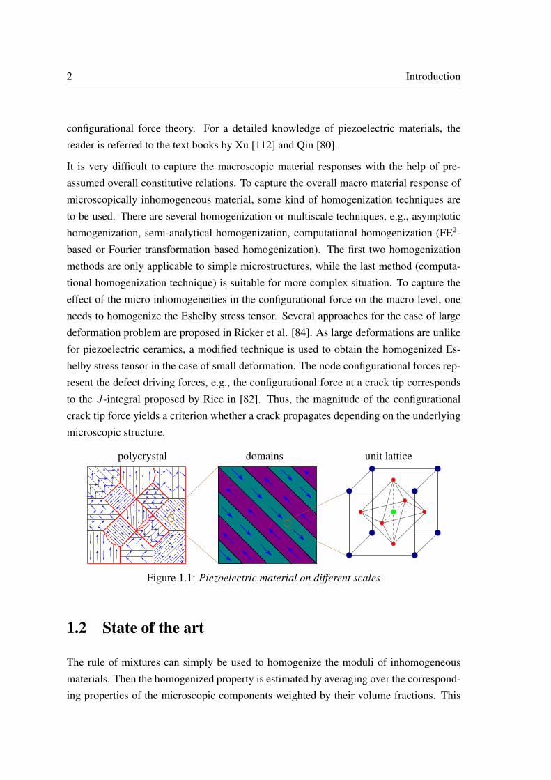
1.1 Piezoelectric material on different scales . . . . . . . . . . . . . . . . . . 2
2.1 Deformation map of reference to actual configuration . . . . . . . . . . . 10
3.1 A representative volume element V R around the point x in electricallycharged continuum body . . . . . . . . . . . . . . . . . . . . . . . . . . 24
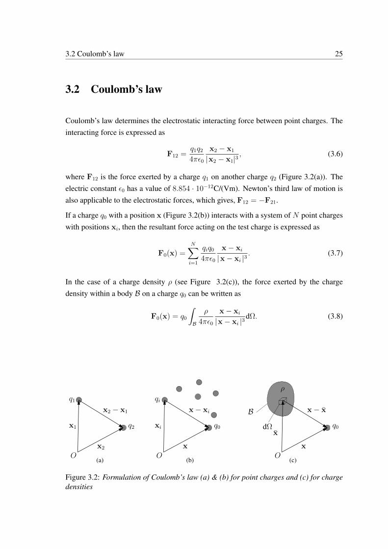
3.2 Formulation of Coulomb’s law (a) & (b) for point charges and (c) forcharge densities . . . . . . . . . . . . . . . . . . . . . . . . . . . . . . . 25
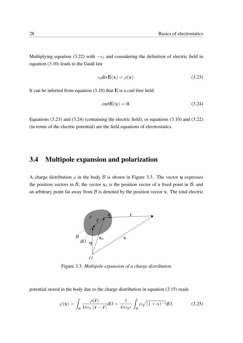
3.3 Multipole expansion of a charge distribution . . . . . . . . . . . . . . . . 28
4.1 A piezoelectric body containing a domain wall . . . . . . . . . . . . . . . 35
5.1 Macro-micro transition . . . . . . . . . . . . . . . . . . . . . . . . . . . 46
5.2 A micro domain or a RVE with the boundary divided into ∂B+mic and ∂B−mic 49
5.3 A fractured macro specimen with dimension h × w containing a sharpcrack (with crack length lc and width at the opening wc), the top of thestructure is displaced by ∆h . . . . . . . . . . . . . . . . . . . . . . . . 58
5.4 Crack tip configurational forces on the macro level produced from (c) &(e) displacement gradient and (b) & (d) strain driven deformation of theinhomogeneous micro domain (a) . . . . . . . . . . . . . . . . . . . . . 59
5.5 Crack tip configurational forces on the macro level produced from (c) &(e) displacement gradient and (b) & (d) strain driven deformation of thehomogeneous micro domain (a) . . . . . . . . . . . . . . . . . . . . . . . 60
5.6 Deformed micro domain with different boundary conditions on the microlevel . . . . . . . . . . . . . . . . . . . . . . . . . . . . . . . . . . . . . 61
5.7 Configurational forces for different microstructures by using displace-ment gradient driven deformation of the micro domain . . . . . . . . . . 62
5.8 Configurational forces for different microstructures by using displace-ment gradient driven deformation of the micro domain . . . . . . . . . . 63
5.9 Configurational forces for different volume fractions of the parts of themicro domain . . . . . . . . . . . . . . . . . . . . . . . . . . . . . . . . 64
5.10 Configurational forces for different ratios of elastic moduli . . . . . . . . 65
v
6.1 A macro domain with dimension h×w contains a sharp crack with cracklength lc and width at opening wc. The top of the structure is displacedwith ∆h and the applied potentials on the top and the bottom are ϕ′ and0, respectively . . . . . . . . . . . . . . . . . . . . . . . . . . . . . . . . 81
6.2 Configurational forces on the domain walls of the microstructure . . . . . 836.3 Stress and electric field distributions on macroscopic specimen: (a) σyy
component of the stress tensor in N/m2, (b) σxx component of the stresstensor in N/m2, (c) Ey component of the electric field in V/m, (d) Excomponent of the electric field in V/m . . . . . . . . . . . . . . . . . . . 84
6.4 Configurational forces for different microstructures without external elec-tric field . . . . . . . . . . . . . . . . . . . . . . . . . . . . . . . . . . . 85
6.5 Configurational forces for different microstructures without an externalelectric field . . . . . . . . . . . . . . . . . . . . . . . . . . . . . . . . . 86
6.6 Configurational forces for different electric loadings using a microstruc-ture which contains vertical domain walls . . . . . . . . . . . . . . . . . 88
6.7 Configurational forces for different electric loading using a microstruc-ture which contains horizontal domain walls . . . . . . . . . . . . . . . . 89
6.8 Configurational forces for different electric loadings using a relativelycomplex microstructure . . . . . . . . . . . . . . . . . . . . . . . . . . . 90
6.9 Absolute value of the configurational forces for different microstructureswith different electric loadings . . . . . . . . . . . . . . . . . . . . . . . 91
6.10 Dependence of configurational forces on the electric field for different ma-terial parameters: (c) polarization and piezoelectric material constant;(d) dielectric material constant . . . . . . . . . . . . . . . . . . . . . . . 92
6.11 Dependence of configurational forces on the electric field for different ma-terial parameters: (c) polarization and piezoelectric material constant;(d) dielectric material constant . . . . . . . . . . . . . . . . . . . . . . . 93
7.1 Kinetics of the domain wall movement . . . . . . . . . . . . . . . . . . . 98
7.2 Determination of new interface position Xn+1S in micro domain . . . . . . 100
7.3 (a) Microstructure used for homogenization, (b) microstructure with thenodal driving forces on the domain wall . . . . . . . . . . . . . . . . . . 102
7.4 Macro specimen . . . . . . . . . . . . . . . . . . . . . . . . . . . . . . . 1037.5 Evolving microstructures at ’Location-1’ and ’Location-2’ at different
nominal applied electric fields . . . . . . . . . . . . . . . . . . . . . . . 1047.6 Percentage of the left domain distribution on the macro specimen at dif-
ferent intensities of nominal electric field . . . . . . . . . . . . . . . . . . 1057.7 (a) Electric displacement using fixed RVE, (b) Electric displacement using
evolving RVE in macro specimen . . . . . . . . . . . . . . . . . . . . . . 1077.8 Comparison of the configurational forces at the crack tip . . . . . . . . . 1087.9 Nominal electric field vs. time on the macro level . . . . . . . . . . . . . 1097.10 Electric displacement vs. time on the macro level . . . . . . . . . . . . . 1107.11 Hysteresis loop (electric displacement vs. electric field) on the macro level 111
vi
Chapter 1
Introduction
1.1 Motivation
Piezoelectric materials, which contain remanent polarizations, feature coupling betweenmechanical and electrical properties. These materials are capable of generating an elec-tric field in response to a mechanical loading. This effect is called direct piezoelectriceffect. In the inverse piezoelectric effect, these materials exhibit a deformation when anexternal electric field is applied. Piezoelectric materials are widely used in sensors andactuators due to their piezoelectric property. Common examples of piezoelectric sensorsare sonic sensors, force and vibration sensors, etc. In valves (e.g., fuel injection, ink-jet)and ultra-sonic motors, piezoelectric materials are used as actuators. Piezoelectric mate-rials are also used in composites and in multi-layer materials to obtain smart solutions ina variety of applications. On the micro level, these materials contain different domainsof polarization, domain walls, grains, grain boundaries, micro cracks, etc. These microfeatures of piezoelectric materials are the source of high inhomogeneities on the microlevel. These inhomogeneities may occur on different scales, see Figure 1.1.
The focus of this work is to study the effects of micro inhomogeneities of piezoelectricmaterials on macroscopic configurational forces. Special effort has been given on theconfigurational forces at certain defect situations. A sharp crack tip is considered as oneof these defect situations. In order to fulfill the task of this research work, one has todeal with three fields of mechanics: electro-mechanically coupled piezoelectric materials;multiscale simulation, or computational homogenization of piezoelectric materials; and
2 Introduction
configurational force theory. For a detailed knowledge of piezoelectric materials, thereader is referred to the text books by Xu [112] and Qin [80].
It is very difficult to capture the macroscopic material responses with the help of pre-assumed overall constitutive relations. To capture the overall macro material response ofmicroscopically inhomogeneous material, some kind of homogenization techniques areto be used. There are several homogenization or multiscale techniques, e.g., asymptotichomogenization, semi-analytical homogenization, computational homogenization (FE2-based or Fourier transformation based homogenization). The first two homogenizationmethods are only applicable to simple microstructures, while the last method (computa-tional homogenization technique) is suitable for more complex situation. To capture theeffect of the micro inhomogeneities in the configurational force on the macro level, oneneeds to homogenize the Eshelby stress tensor. Several approaches for the case of largedeformation problem are proposed in Ricker et al. [84]. As large deformations are unlikefor piezoelectric ceramics, a modified technique is used to obtain the homogenized Es-helby stress tensor in the case of small deformation. The node configurational forces rep-resent the defect driving forces, e.g., the configurational force at a crack tip correspondsto the J-integral proposed by Rice in [82]. Thus, the magnitude of the configurationalcrack tip force yields a criterion whether a crack propagates depending on the underlyingmicroscopic structure.
polycrystal domains unit lattice
Figure 1.1: Piezoelectric material on different scales
1.2 State of the art
The rule of mixtures can simply be used to homogenize the moduli of inhomogeneousmaterials. Then the homogenized property is estimated by averaging over the correspond-ing properties of the microscopic components weighted by their volume fractions. This
1.2 State of the art 3
method provides a rough estimate of the overall property by considering only a single mi-crostructural characteristic, namely the volume fractions in the inhomogeneous material.This method does not include the influences of other microstructural characteristics. Atechnique is presented in Voigt [107] and Reuss [81] in order to estimate the upper andlower bounds of the macroscopic moduli. More accurate bounds for overall propertiesusing a variational formulation are discussed in Hashin and Shtrikman [35, 36, 37].
A better technique is given in Eshelby [15], where the analytical solution of a boundaryvalue problem of a spherical or an elliptical inclusion material in an infinite matrix isconsidered to determine the effective material parameters. This is the so called equivalenteigenstrain method. The extension of this method is the so called self-consistent method.In this method a particle of one phase is embedded into a material with unknown effectivematerial properties. This approach is suitable for microstructures with regular geometry.This method is used for polycrystalline ceramics in the work by Kröner [50]. Readersare referred to Hashin [33, 34], Hill [39], Willis [110], etc. for more consultation on theself-consistent method. Another analytical homogenization method is presented in thearticle of Mori and Tanaka [68], Tanaka and Mori [102] and Benveniste [6] by using themean-field approximation. This method is known as the Mori-Tanaka method.
An asymptotic homogenization procedure is outlined in Bensoussan et al. [5] and Sanchez-Palencia [85]. In this method an asymptotic expansion of the displacement and stressfields is applied on the ratio of a characteristic size of the heterogeneities and a measure ofthe microstructure, see Toledano and Murakami [103], Devries et al. [13], Suquet [100],Guedes and Kikuchi [30], Fish et al. [20]. This asymptotic homogenization method issuitable for the determination of effective overall properties as well as the local stress andstrain quantities. The weakness of this method is that it is only applicable to a problemwith simple micro domain and simple material models, generally for small deformations.
The so called unit cell methods are developed in order to handle the increasing inho-mogeneities and complexities in the microstructures. These approaches are mentionedin different publications, e.g., Christman et al. [12], Bao et al. [4], Suresh et al. [101],Nakamura and Suresh [75], McHugh et al. [59], and so on. These unit cell methods arecapable to supply valuable information on the local microstructural fields along with thehomogenized material properties. The material properties are usually calculated by fittingthe homogenized microscopical stress-strain fields, which are estimated from the analysisof a microstructural representative cell subjected under a certain loading, on macroscopi-cally closed form phenomenological constitutive relations in a predetermined format. It is
4 Introduction
severely difficult to prepare a suitable assumption for the macroscopic constitutive formatif the material behavior shows nonlinearities. The unit cell method is used in the workof Poizat and Sester [78] and Li et al. [54], where effective properties of piezoelectricmaterials or composites are calculated.
Recently, an encouraging numerical method to homogenize the microscopically inho-mogeneous engineering material has been developed, i.e. the multiscale computationalhomogenization. This approach is documented in the articles by Suquet [100], Guedesand Kikuchi [30], Terada and Kikuchi [104], Ghosh et al. [25, 26]; and further de-veloped and improved in more recent years by Smit et al. [98], Miehe et al. [66, 67],Michel et al. [62], Feyel and Chaboche [19], Terada and Kikuchi [105], Ghosh et al. [27],Kouznetsova et al. [49], Miehe and Koch [65]. These micro-macro modeling methodsevaluate the stress-strain at every point of interest on the macro level by an elaborate mi-crostructural modeling attached to that macro point. This type of multiscale modelingdoes not necessitate a constitutive law on the macro level, and is capable to handle largedeformation on the macro and on the micro levels. This method is suitable for any ma-terial law, physical nonlinearity and time dependency. The finite element method can beused to model the micro domain, see Smit et al. [98], Feyel and Chaboche [19], Teradaand Kikuchi [105], and so on. If both macro and micro scales are simulated with the helpof finite elements, the method is called FE2-based computational homogenization. Thisis the interest of this research work. A detailed illustration of this approach can be foundin Feyel [17, 18], Feyel and Chaboche [19], Miehe and Koch [65], Miehe [63, 64]. Inthe work of Ricker et al. [83, 84], a FE2-based computational homogenization is used tohomogenize the Eshelby stress tensor and the configurational forces. An application ofthis FE2-based method towards the piezoelectric materials can be found in Schröder andKeip [92, 93, 94], Keip and Schröder [44]. In the work of Khalaquzzaman et al. [47], aFE2-based homogenization technique is used in order to homogenize the configurationalforces of piezoelectric materials. Few more numerical homogenization methods incorpo-rating Voronoi cell methods are documented in publications of Ghosh et al. [25, 26],and methods based on fast Fourier transformation are presented in Fotiu and Nemat-Nasser [22], Moulinec and Suquet [69] and Miehe et al. [67].
A detailed survey of homogenization approaches can be found in the articles by Kanouté[43] and Geers et al. [24]. A comprehensive overview of homogenization methods iselaborated in the text books by Gross and Seelig [29] or Nemat-Nasser and Hori [76].
1.3 Structure of the investigation 5
Primarily, the idea of the energy-momentum tensor to continuum mechanics of solids wasdiscussed by Eshelby in Eshelby [14]. However, at that time the term energy-momentumtensor was not used. It was described as the Maxwell-tensor of elasticity. Later in Es-helby [16], the term energy-momentum tensor was introduced. Configurational force,which indicates the energy changes in a system, is a convenient tool to investigate theinhomogeneities or the fracture of solids. Further, this abstract physical quantity is alsoused in refinement of finite element meshes in Müller and Maugin [74], Müller et al. [73]and Braun [8]. To get a broad idea on configurational forces, the reader is referred tosome well established text books, e.g., Maugin [58], Kienzler and Herrmann [48] andGurtin [32].
The evolution of the microstructure of piezoelectric materials can be modeled by a sharpinterface approach, or by a phase field approach. By modeling the domain wall with asharp interface approach, a jump in certain material properties is introduced. As a re-sult, the theory of configurational forces is applicable to the evolution of microstructures.In the work by Loge and Suo [56], a set of generalized coordinate systems was intro-duced to capture the geometry of the domain state, and a linear kinetic law, which isbased on a variational principle, connects the rates of these coordinates to the conjugatedriving force. The driving force is formulated within a thermodynamic framework inKessler and Balke [45, 46], where the bending of domain walls is addressed. By usingthe driving force on the interface, a kinetic law for domain wall movement is postulatedin Müller et al. [72] and Schrade et al. [88].
Phase field approaches regarding domain evolution in ferroelectric materials are discussedin Cao et al. [9], Wang et al. [109], Ahluwalia and Cao [1], Ahluwalia et al. [2], Choud-hury et al. [10], Zhang and Bhattacharya [113], and Choudhury et al. [11]. A detailednumerical treatment of the complete set of equations of domain evolution is presentedin Su and Landis [99], and Wang and Kamlah [108], where the finite element method isused. Phase field models, which incorporate the spontaneous polarization as the orderparameter, are presented in Schrade et al [87, 89, 90].
1.3 Structure of the investigation
This research work is subdivided into six chapters. For the sake of completeness, a briefintroduction of continuum mechanics and electrostatics is given in Chapter 2 and Chap-
6 Introduction
ter 3, respectively. Section 2.1 - 2.4 gives a short overview of continuum mechanics ina large deformation setting. It covers kinematics of deformation, strain measures, stressmeasures and balance laws in continuum mechanics. Since piezoelectric materials ex-hibit only small deformation, in Section 2.5 kinematics of deformation, strain measures,stress measures, and balance laws are recasted in a small strain setting. The theory ofconfigurational forces is presented in Section 2.6
In Section 3.1 - 3.4 a short overview of the electric charge, Coulomb’s law, the electricpotential, and the electric polarization in vacuum are given. Section 3.5 provides a shortoverview of the corresponding formulation of electrostatics in matter.
The theory of piezoelectric materials is presented in Chapter 4. It provides the fieldequations and the constitutive law of piezoelectric materials which includes the electro-mechanical coupling. In Section 4.3 the numerical implementation of the boundary valueproblem (BVP) regarding piezoelectric materials is concisely discussed. A detailed deriva-tion of configurational forces for piezoelectric materials and a brief description on thenumerical treatment of configurational forces are presented in Section 4.4.
Chapter 5 provides a detailed formulation of the FE2-based homogenization techniques ina small strain framework using the configurational force theory. All derivations presentedin this chapter are given only for the mechanical response of the material. In Section 5.1.1a new set of boundary conditions for the micro boundary value problem is derived. Adetailed derivation and discussion of different homogenization techniques of the Eshelbystress tensor are presented in Section 5.2. At the end of this chapter, numerical resultsare presented. In particular, crack tip configurational forces on the macro level, whichare determined by using different microstructures, are obtained. The investigations in thischapter play a supporting role in the homogenization of piezoelectric materials in the nextchapter.
Chapter 6 provides a detailed description of the FE2-based homogenization techniquesof piezoelectric materials using the configurational force theory. An detailed discussionof admissible boundary conditions for the micro BVPs is presented in Section 6.1. Thedetermination of homogenized material moduli of piezoelectric materials is given in Sec-tion 6.2. Numerical results regarding configurational forces at the crack tip are also pre-sented. Different micro structures and different electrical loadings are considered. Allsimulations in this chapter are carried out using non-evolving or stationary microstruc-tures.
1.3 Structure of the investigation 7
The treatment of homogenization techniques of piezoelectric materials using evolvingmicrostructures is given in Chapter 7. It provides the theoretical background of the influ-ences of external loadings on the underlying microstructures of piezoelectric materials.The evolution of the microstructures is realized with the help of configurational forces inthe micro domain. Numerical results of the macro electric displacement distribution, thescale of evolution in the micro structure, the hysteresis in piezoelectric materials on themacro level are presented in this chapter.
Chapter 8 delivers a short conclusion of this research work and recommendations onfuture topics.

8 Introduction
Chapter 2
Basics of continuum mechanics
Continuum mechanics is an important branch of mechanics. It helps us to deal withmaterial simulations and structural problems to capture the mechanical responses. Incontinuum mechanics the modeling of the material is done as continuous mass ratherthan as discrete particles. At the beginning of this chapter, a short overview of non-linear continuum mechanics will be provided. Afterwards all relevant relations for linearcontinuum mechanics will be reformulated. Several textbooks could be listed on theclassical continuum mechanics. Without claiming completeness some of them are listedas reference for the readers: Holzapfel [40], Ogden [77], Haupt [38], Gurtin [31], Marsdenand Hughes [57], Fung and Tong [23], Betten [7], Liu [55].
2.1 Kinematics of deformation
The transformation of a continuum body from a reference or undeformed configurationto the current or spatial configuration is represented in Figure 2.1. The symbols B0 andB represent the continuum body in the undeformed configuration and in the spatial con-figuration, respectively. The one-to-one non-linear mapping function χ(·) in Figure 2.1defines the motions of a continuum body,
x = χ(X, t) (2.1)
which maps material points (denoted by the position vector X in the undeformed con-figuration) to the points in the current configuration denoted by the position vector x at
10 Basics of continuum mechanics
X
x
B0
B
dX
dΩNdΓ dv
nda
dx
reference configuration actual configurationχ(X, t)
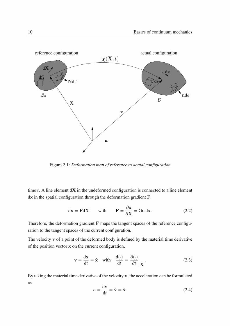
Figure 2.1: Deformation map of reference to actual configuration
time t. A line element dX in the undeformed configuration is connected to a line elementdx in the spatial configuration through the deformation gradient F,
dx = FdX with F =∂x
∂X= Gradx. (2.2)
Therefore, the deformation gradient F maps the tangent spaces of the reference configu-ration to the tangent spaces of the current configuration.
The velocity v of a point of the deformed body is defined by the material time derivativeof the position vector x on the current configuration,
v =dx
dt= x with
d(·)dt
=∂(·)∂t
∣∣∣∣X. (2.3)
By taking the material time derivative of the velocity v, the acceleration can be formulatedas
a =dv
dt= v = x. (2.4)
2.2 Strain measures 11
One can define the spatial velocity gradient l, which has an important role to describemotions as
l = gradv =∂v
∂x= FF−1 = −FF−1. (2.5)
To describe the transformation and the rate of a line element dx, a surface element nda,and a volume element dv, the deformation gradient F and the spatial velocity gradient l
are the required kinematic quantities. The relations are summarized as
dx = FdX, dx = ldx,
nda = JF−TNdΓ, (nda). =[(divv)1− lT
]nda,
dv = JdΩ, dv = (divv)dv = (trl)dv,
(2.6)
where J is the determinant of the Jacobian of the non-linear mapping, i.e. J = detF.
2.2 Strain measures
With the help of the polar decomposition, it is possible to decompose the deformationgradient F in two ways: with a proper orthogonal rotation tensor R and a symmetricright stretch tensor U, or with a symmetric left stretch tensor V and a rotation R. Thedecomposition is done in the following way:
F = RU = VR, (2.7)
with U = UT , V = VT , RRT = 1, detR = 1.
It is convenient to define the strain measures with the right and left stretch tensors U andV. These stretch tensors are involved in the description of the deformation of a continuumbody. Commonly used deformation tensors, which are based on U and V, are given asexample in the following:
C = FTF = UTU = U2 right Cauchy-Green tensor, (2.8)
b = FFT = VVT = V2 left Cauchy-Green tensor. (2.9)
12 Basics of continuum mechanics
In the undeformed or reference state (F = 1), a strain measure should be zero. Makinguse of this idea leads to the introduction of the frequently used strain measures in thefollowing:
E =1
2(C− 1) Green-Lagrange strain tensor,
e =1
2(1− b−1) Euler-Almansi strain tensor.
(2.10)
The Green-Lagrange and the Euler-Almansi strain tensor are related by deformation gra-dient F in the following way:
FTeF = E. (2.11)
Both strain tensors show the stretching of a line element of the continuum body in thereference configuration during deformation. This can be seen considering
ds2 − dS2 = dx · dx− dX · dX = dX · (2EdX) = dx · (2edx). (2.12)
The rate of change of a line element in the undeformed configuration can be expressed as
ddt
(ds2 − dS2) = 2dx · (ddx) = 2dx ·[(e + lTe + el)dx
]= 2dX · (EdX), (2.13)
where d denotes the symmetric part of the spatial velocity gradient which is defined bythe additive split of l in the following way:
l = d + w with d =1
2(l + lT ) and w =
1
2(l− lT ). (2.14)
2.3 Stress measures
Using the stress tensors σ and P, the traction vectors t and T, which are defined as forceper area in the actual and reference configuration, respectively, can be formulated by alinear mapping of the normal vectors n and N, respectively. The normal vectors n and N
are also defined in the actual and reference configuration, respectively. As a consequence,one obtains
TdΓ = PNdΓ = tda = σnda. (2.15)
The stress tensors P and σ are named as the first Piola-Kirchhoff stress and the Cauchystress tensor, respectively. As the first Piola-Kirchhoff stress tensor is in the actual and the
2.4 Balance laws 13
reference configurations, it is identified as a so called two field tensor. On the other hand,the Cauchy stress tensor is defined completely in the actual configuration and shows thesymmetry property σ = σT for a simple continuum. With the help of (2.63) these twostress tensors can be related in the following way:
P = JσF−T , (2.16)
and the following identity is established by using the symmetry property of the Cauchystress tensor
PFT = FPT . (2.17)
The first Piola-Kirchhoff stress tensor does not have the symmetry property as the Cauchystress tensor. For that reason, the second Piola-Kirchhoff stress tensor S is introduced toobtain a symmetric stress measure defined in the reference configuration. The secondPiola-Kirchhoff stress tensor can be defined by
S = F−1P = JF−1σF−T yielding S = ST . (2.18)
2.4 Balance laws
The concept of balance laws plays an important role in the understanding of continuummechanics as well as the theory of configurational forces. In continuum mechanics fivebalance laws need to be formulated, namely the balance of mass, of linear momentum,of angular momentum, of energy, and of entropy. Any balance law listed here has thegeneralized structure
ddt
∫
B0
ϕdΩ =
∫
∂B0
Φ ·NdΓ +
∫
B0
rϕdΩ, (2.19)
where ϕ is the quantity which needs to be balanced, rϕ is the supply/production of ϕ andΦ is the flux of ϕ. Equation (2.19) is stated for a control volume B0 (in the undeformedconfiguration). Therefore, it is termed as a global balance law. Equation (2.19) can betransformed to its local form with the help of the Gauß theorem in the following way:
ϕ = DivΦ + rϕ. (2.20)
14 Basics of continuum mechanics
The mass balance, or precisely termed as the conservation of mass, can be written inglobal and local form in the reference or in the undeformed configuration by
ddt
∫
B0
ρ0dΩ = 0 or ρ0 = 0, (2.21)
respectively. Here ρ0 denotes the mass density of the continuum in the reference config-uration. By making use of (2.65), the mass density in the reference configuration ρ0 andthe density in the current configuration ρ can be related by
∫
B0
ρ0dΩ =
∫
Bρdv ⇒ ρ0 = ρJ. (2.22)
The balance of linear momentum is expressed by
ddt
∫
B0
ρ0vdΩ =
∫
∂B0
PNdΓ +
∫
B0
fdΩ (2.23)
in the global form, and in the local form it is defined by
ρ0v = DivP + f , (2.24)
where f expresses the body forces which are defined per volume in the reference config-uration.
In the static condition the inertia terms can be neglected. As a result, this leads to theequilibrium conditions in the global and local form
∫
∂B0
PNdΓ +
∫
B0
fdΩ = 0, (2.25)
andDivP + f = 0, (2.26)
respectively.
The following balance law in the global form
ddt
∫
B0
x× (ρ0v)dΩ =
∫
∂B0
x× (PN)dΓ +
∫
B0
x× fdΩ (2.27)
2.4 Balance laws 15
holds for the angular momentum. The global balance of angular momentum leads to theequation (2.17) in the local form, which is analogous to the symmetry of the Cauchy stresstensor σ = σT .
The balance of energy for a control volume in the reference configuration is expressed by
ddt
∫
B0
ρ0(e+1
2v·v)dΩ =
∫
∂B0
(PN)·vdΓ+
∫
B0
f ·vdΩ−∫
∂B0
Q·NdΓ+
∫
B0
rdΩ, (2.28)
where e, Q and r are the internal energy, the heat flux and source, respectively. Theenergy balance in the local form can be written as
ρ0e = P : F− DivQ + r. (2.29)
The balance of entropy in the global form can be written as
ddt
∫
B0
ρ0sdΩ = −∫
∂B0
Q
T·NdΓ +
∫
B0
r
TdΩ +
∫
B0
ΠsdΩ, (2.30)
where s is the entropy of the system, the entropy flux is given by Q/T and the entropysource by r/T , with T the absolute temperature. The entropy production is designatedby Πs. The entropy s determines the direction in which thermodynamic processes takeplace. The local form of the entropy balance is written as
ρ0s = −Div(
Q
T
)+r
T+ Πs. (2.31)
From the second law of thermodynamics, it can be inferred that the entropy production Πs
has always a non-negative value,Πs ≥ 0. (2.32)
To deal with the purely mechanical theory of a system, the elimination of the heat flux Q
and the heat production r in equations (2.28) and (2.30) or in equations (2.29) and (2.31)is to be done by introducing the free Helmholtz energy w. It is assumed that the changesin the state of the system are isothermal. As a result, the reduced dissipation inequality
D = ΠsT = P : F− ρ0w ≥ 0 with w = e− Ts (2.33)
is obtained.
16 Basics of continuum mechanics
A free Helmholtz energy per volume in the reference or undeformed configuration isexpressed by
W = ρ0w, (2.34)
where W is also denoted as strain energy. The strain energy W can be considered as apotential for the stress measures because of the following equations:
P =∂W
∂For S =
∂W
∂E= 2
∂W
∂C. (2.35)
2.5 Small deformations
The basics of continuum mechanics presented in the previous sections enable us to in-troduce the basic theory of configurational forces in the large strain framework. Since inpiezoelectric materials there are only small deformations, it is not necessary to use thelarge strain formulation. In this situation a geometrically linear theory of continuum bodyserves the purpose. The central idea to derive the kinematically linear theory is based onthe assumption that the current and the reference configuration approximately coincide.This assumption may create confusions when formulating the configurational force the-ory, as it is founded on changes of the continuum body in the reference configuration.On the other hand, the classical physical forces are based on changes in the actual con-figuration. In the case of large strain theory, a material point is denoted by its positionin the undeformed configuration X (name of the particle). In small deformation settinga material point is designated just by its position or its coordinates x. The displacementvector u defined by
u = x−X (2.36)
plays an important role as an essential kinematic descriptor in this theory. Within smallstrain theory, all stress and strain measures become identical. The linearized strain ε isdefined as
ε =1
2(∇u + (∇u)T ), (2.37)
and the stress tensor is denoted by σ. The velocity v is defined as u. According to thesmall deformation setting it is not required to have two different control volumes in thereference and in the actual configuration. Furthermore no distinction between ρ and ρ0 isrequired. The density is simply denoted by ρ in the following.
2.5 Small deformations 17
One can present all previous balance laws for small strain (geometric linear) setting in ashort list,
1. conservation of massρ = const., (2.38)
2. balance of linear momentum
ddt
∫
BρudΩ =
∫
∂BσndΓ +
∫
BfdΩ (2.39)
orρu = divσ + f , (2.40)
3. balance of angular momentum
ddt
∫
Bx× (ρu)dΩ =
∫
∂Bx× (σn)dΓ +
∫
Bx× fdΩ (2.41)
orσ = σT , (2.42)
4. balance of energy
ddt
∫
Bρ
(e+
1
2| u |2
)dΩ =
∫
∂B(σn)·udΓ+
∫
Bf ·udΩ−
∫
∂BQ·ndΓ+
∫
BrdΩ (2.43)
orρe = σ : ε− divQ + r, (2.44)
5. balance of entropy
ddt
∫
BρsdΩ = −
∫
∂B
Q
T· ndΓ +
∫
B
r
TdΩ +
∫
BΠsdΩ (2.45)
orρs = −div
(Q
T
)+r
T+ Πs, (2.46)
6. second law of thermodynamicsΠs ≥ 0. (2.47)
18 Basics of continuum mechanics
The reduced dissipation inequalities becomes
D = σ : ε− W ≥ 0, (2.48)
which leads by standard arguments to the conclusion that
σ =∂W
∂ε. (2.49)
2.6 Configurational forces
The theory of configurational forces provides a convenient mechanism to investigate dif-ferent kinds of material defects. In the literature configurational forces are also calledmaterial forces. This theory provides an unified approach to investigate defects and pro-cesses that bring changes in the material structure. It is frequently applied in the fields offracture mechanics and phase transformations.
The theory of configurational forces with appropriate formulations can be used to modelpoint, line, area and volume defects. Physically point defects may represent interstitialatoms or vacancies (centers of dilatation); dislocation lines may be considered as linedefects; interfaces may be represented as area defects; and inclusions may be modeledas volume defects. Configurational forces play an important role in the analysis of mor-phology changes, which is very important for material science, as the macro constitutiveresponse is greatly affected by the arrangement and evolution in the microstructures, seee.g., Müller and Gross [70, 71]. Driving forces are formulated with the consideration ofthe change of the total potential with respect to a virtual motion of the defect in the ref-erence configuration. This fact is used in all applications of configurational forces. Thematerial or configurational forces in continuum mechanics were introduced by Eshelbyin the early fifties of the last century. In Eshelby [14] the driving forces on elastic sin-gularities were evaluated via a second-order tensor (at that time Eshelby did use the term’Maxwell tensor of elasticity’). Eshelby proved that the negative gradient of the total po-tential with respect to the position of the defect can be suitably used for the evaluation ofmaterial imperfections.
2.6 Configurational forces 19
2.6.1 Theory of configurational forces
The theory of configurational forces, which is presented in the following, follows the in-troductory ideas stated in Eshelby [14, 16]. For a concise derivation only elastic materialsare taken into consideration, but an extension of this derivation is possible for inelasticsettings and has been discussed elaborately in Maugin [58]. For the theoretical analysisour attention is restricted to the quantities that are defined with respect to the materialconfiguration in an effort to make the derivations more condensed. There exists a strainenergy function
W = W (F,X) (2.50)
per unit volume of a hyper-elastic material in the reference configuration. An assumptionis made that W depends on the deformation gradient F and explicitly on the positionvector X (in the reference configuration). The second dependency is taken into accountin order to be able to consider heterogeneity in the material. The first Piola-Kirchoff stresstensor is calculated by
P =∂W
∂F. (2.51)
For static conditions the balance of momentum (2.23) can be written in its local form as
DivP + f = 0, (2.52)
see equation (2.26). The vector f denotes body forces (defined per unit volume of the ref-erence configuration). One can express the material gradient of the strain energy functionW as in the following
GradW = P : GradF +∂W
∂X
∣∣∣∣∣expl.
(2.53)
= Div(FTP)− FTDivP +∂W
∂X
∣∣∣∣∣expl.
.
The first term on the RHS of (2.531) can be expressed in index notation by PiJFiJ,K . Thesubscript expl. appearing for the first time in the second term in (2.531) indicates the ex-plicit derivative of W with respect to the position X. Mathematical manipulations and in-
20 Basics of continuum mechanics
corporation of the mechanical equilibrium condition (2.52) and kinematics F = ∂x/∂X
lead to an equation for the material forces in the form
Div Σ + g = 0, (2.54)
where the Eshelby stress tensor or the energy-momentum tensor is defined by
Σ = W1− FTP, (2.55)
and the configurational force
g = −FT f − ∂W
∂X
∣∣∣∣∣expl.
(2.56)
is introduced in order to obtain a similar structure as that of equation (2.52). With thedefinition of the symmetric Piola-Kirchhoff stress tensor in (2.18) and the symmetric rightCauchy-Green tensor in (2.8), equation (2.55) can be expressed as
Σ = W1−CS, thus, ΣC = CΣT . (2.57)
The last expression in equation (2.57) can be considered as the symmetry of the Eshelbystress tensor Σ with respect to right Cauchy-Green tensor C. From (2.56) an importantrealization can be drawn: if a continuum body is homogeneous and it does not containany body forces, the divergence of the Eshelby stress tensor disappears, and that leads to
DivΣ = 0. (2.58)
It can be stated that the Eshelby stress tensor satisfies a conservation law strictly withinthe continuum body. For an elaborate discussion of conservation laws of the Eshelbystress tensor, Kienzler and Herrmann [48] can be consulted.
2.6.2 Configurational forces in small deformation
In the previous section the configurational forces for large deformation problems are de-scribed. Since the piezoelectric materials investigated in this work exhibit primarily smalldeformation, a brief description of the configurational forces for the small deformation
2.6 Configurational forces 21
setting will be discussed. The concept of configurational forces within a small deforma-tion framework is a bit confusing, as the current configuration coincides with referenceconfiguration in a small deformation framework.
Similar to large deformations, one can write the balance of configurational forces forsmall deformation problems as
div Σ + g = 0. (2.59)
The Eshelby stress tensor is defined as
Σ = W1− (∇u)Tσ, (2.60)
and volume configurational forces are defined as
g = −(∇u)T f − ∂W
∂x
∣∣∣∣∣expl.
. (2.61)
For a complete derivation of the balance of configurational forces, the Eshelby stresstensor and the volume configurational forces in a small deformation framework, the readeris referred to Kienzler and Herrmann [48] and Müller et al. [73].
22 Basics of continuum mechanics
Chapter 3
Basics of electrostatics
Electrostatics is an important field of study in physical science incorporating the prop-erties and phenomena of static charges, or of charges with slow movement and in theabsence of acceleration. In this chapter a very short overview of electrostatics is pre-sented, where electrodynamics and magnetic behavior of moving charges are neglected.Textbooks on the theories of electrostatics and -dynamics include Landau and Lifshitz [51,52], Purcell [79] and Jackson [42]; a brief summary can be found in Schrade [86], Goy [28]and Mehling [61].
3.1 Electric charge
Electric charge, which has an influence on electromagnetic interaction, is a conservedproperty of particles. Modern experiments show that the electric charge is a quantizedquantity. Being a quantized quantity, it can only contain values of integer multiples ofthe elementary charge e ≈ 1.60217646 · 10−19 C. The proton and the electron havethe charge of e and −e, respectively. Due to the additive feature, N electrically chargedparticles with individual charges qi have the total charge
q =N∑
i=1
qi. (3.1)
24 Basics of electrostatics
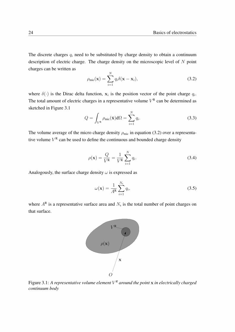
The discrete charges qi need to be substituted by charge density to obtain a continuumdescription of electric charge. The charge density on the microscopic level of N pointcharges can be written as
ρmic(x) =N∑
i=1
qiδ(x− xi), (3.2)
where δ(·) is the Dirac delta function, xi is the position vector of the point charge qi.The total amount of electric charges in a representative volume V R can be determined assketched in Figure 3.1
Q =
∫
V Rρmic(x)dΩ =
N∑
i=1
qi. (3.3)
The volume average of the micro charge density ρmic in equation (3.2) over a representa-tive volume V R can be used to define the continuous and bounded charge density
ρ(x) =Q
V R =1
V R
N∑
i=1
qi. (3.4)
Analogously, the surface charge density ω is expressed as
ω(x) =1
AR
Ns∑
i=1
qi, (3.5)
where AR is a representative surface area and Ns is the total number of point charges onthat surface.
O
x
ρ(x)
V R
Figure 3.1: A representative volume element V R around the point x in electrically chargedcontinuum body
3.2 Coulomb’s law 25
3.2 Coulomb’s law
Coulomb’s law determines the electrostatic interacting force between point charges. Theinteracting force is expressed as
F12 =q1q2
4πε0
x2 − x1
|x2 − x1|3, (3.6)
where F12 is the force exerted by a charge q1 on another charge q2 (Figure 3.2(a)). Theelectric constant ε0 has a value of 8.854 · 10−12C/(Vm). Newton’s third law of motion isalso applicable to the electrostatic forces, which gives, F12 = −F21.
If a charge q0 with a position x (Figure 3.2(b)) interacts with a system of N point chargeswith positions xi, then the resultant force acting on the test charge is expressed as
F0(x) =N∑
i=1
qiq0
4πε0
x− xi|x− xi |3
. (3.7)
In the case of a charge density ρ (see Figure 3.2(c)), the force exerted by the chargedensity within a body B on a charge q0 can be written as
F0(x) = q0
∫
B
ρ
4πε0
x− xi|x− xi |3
dΩ. (3.8)
(a) (b) (c)
q1
x1
x2
q2
x2 − x1
O
qi
xi
x
q0
x− xi
O
ρ
x
x
q0
x− x
O
BdΩ
Figure 3.2: Formulation of Coulomb’s law (a) & (b) for point charges and (c) for chargedensities
26 Basics of electrostatics
The electric field is defined as the electrostatic force acted on a unit point charge. Equa-tions (3.7) and (3.8) lead to the expression of the electric field E due to a system of pointcharges and a charged continuous body
E(x) =N∑
i=1
qi4πε0
x− xi|x− xi |3
and E(x) =
∫
B
ρ
4πε0
x− xi|x− xi |3
dΩ, (3.9)
respectively.
3.3 Work and electric potential
As the electric field is a conservative quantity, it can be expressed by a scalar potentialfield
E(x) = −∇ϕ(x), (3.10)
where ∇ϕ expresses the gradient of the electric potential. The electrostatic force on acharge is expressed as
F0 = q0E. (3.11)
In order to move a charge q0 from a point P with position vector xP to another point Lwith position vector xL along an arbitrary path Γ, the following work is required
WLP = −
∫
Γ
F0 · ds = −q0
∫
Γ
E · ds (3.12)
= q0
∫
Γ
∇ϕ(x) · ds = q0(ϕ(xP )− ϕ(xL)). (3.13)
The scalar field ϕ is named the electric potential and is unique up to a constant whichis often set to zero. The electric potential for the system of point charges depicted inFigure 3.2(b) is
ϕ(x) =N∑
i=1
qi4πε0 |x− xi |
, (3.14)
and the electric potential for the charge distribution shown in Figure 3.2(c) is given by
ϕ(x) =
∫
B
ρ(x)
4πε0 |x− x |dΩ. (3.15)
3.3 Work and electric potential 27
The total potential energy of a system of point charges considering only its own electricfield is given by
U =1
2
N∑
i=1
N∑
j=1i 6=j
qiqj4πε0 |xi − xj |
, (3.16)
and equation (3.16) can be written using the definition of the potential in (3.14) as
U =1
2
N∑
i=1
qiϕ(xi). (3.17)
In the case of a charge distribution, the total potential can be written as
U =1
2
∫
B
∫
B
ρ(x)ρ(x)
4πε0 | x− x |dΩdΩ (3.18)
and similarly, equation (3.18) can be written by using the definition of the potential in(3.15) as
U =1
2
∫
Bϕ(x)ρ(x)dΩ. (3.19)
The total potential energy of a collection of N discrete charges placed in an externalelectric potential field ϕext is
Uext =N∑
i=1
qiϕext(xi), (3.20)
where the effect of the electric fields due to the charges qi of the system is not considered.For a charge distribution, the total potential can be expressed by
Uext =1
2
∫
Bϕext(x)ρ(x)dΩ. (3.21)
Gauß law:From equation (3.15) it follows that
∆ϕ(x) =1
ε0
∫
Bρ(x)∆
1
4π |x− x |dΩ = − 1
ε0
∫
Bρ(x)δ(x− x)dΩ = −ρ(x)
ε0, (3.22)
where ∆ is the Laplace operator.
28 Basics of electrostatics
Multiplying equation (3.22) with −ε0 and considering the definition of electric field inequation (3.10) leads to the Gauß law
ε0divE(x) = ρ(x). (3.23)
It can be inferred from equation (3.10) that E is a curl free field:
curlE(x) = 0. (3.24)
Equations (3.23) and (3.24) (containing the electric field), or equations (3.10) and (3.22)(in terms of the electric potential) are the field equations of electrostatics.
3.4 Multipole expansion and polarization
A charge distribution ρ in the body B is shown in Figure 3.3. The vector η expressesthe position vectors in B, the vector x0 is the position vector of a fixed point in B, andan arbitrary point far away from B is denoted by the position vector x. The total electric
O
xx0
ηdΩB
ρ nr
r
Figure 3.3: Multipole expansion of a charge distribution
potential stored in the body due to the charge distribution in equation (3.15) reads
ϕ(x) =
∫
B
ρ(r)
4πε0 |r− r |dΩ =1
4πε0r
∫
Bρ√
(1 + α)−1dΩ, (3.25)
3.5 Electrostatics in matter 29
where α is defined as r−2(r2−2r · r) 1; the vectors r = x−x0 = rn and r = η−x0 =
rn are defined in such a way that x−η = r− r. The multipole expansion of ϕ in equation(3.25) can be written as
ϕ(x) =1
4πε0
[1
r
∫
Bρ(r)dΩ +
n
r2·∫
Bρ(r)rdΩ +
n⊗n
2r3:
∫
Bρ(r)(3r⊗r− r1)dΩ + ...
](3.26)
by using the Taylor series expansion of√
(1 + α)−1 with respect to α around α = 0. TheTaylor expansion of (1 + α)−
12 is 1− 1
2α + 3
8α2 − 5
16α3 + ....
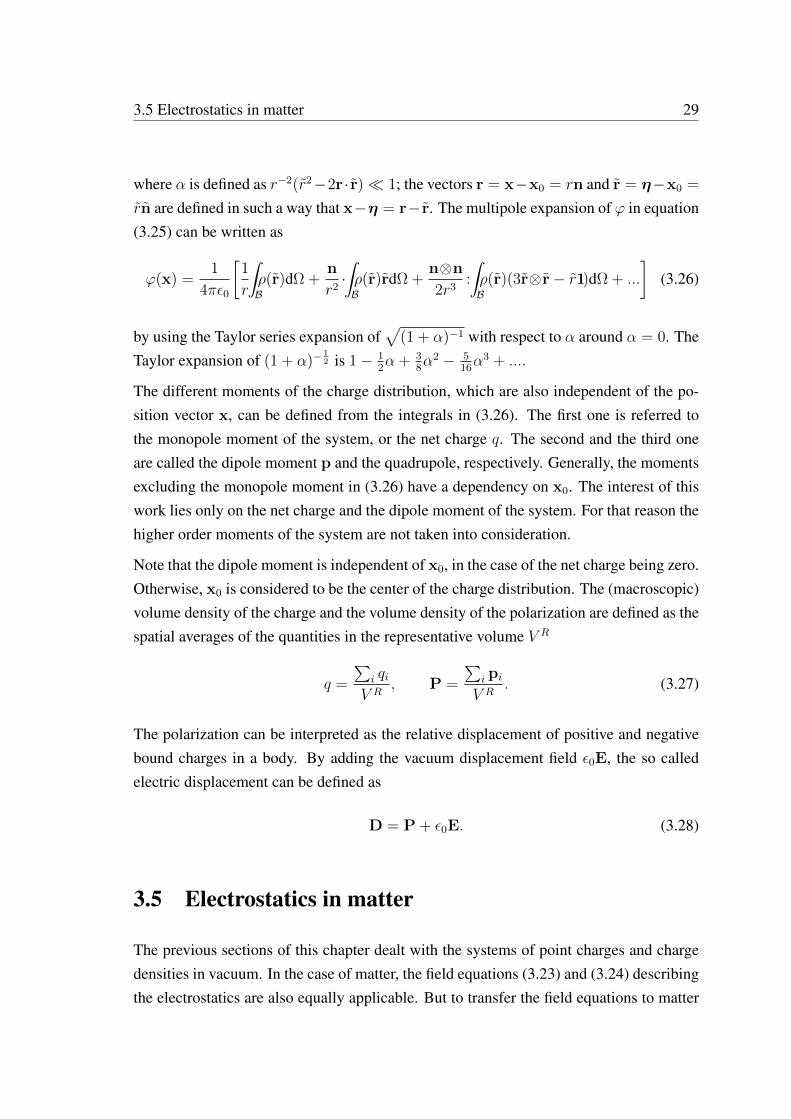
The different moments of the charge distribution, which are also independent of the po-sition vector x, can be defined from the integrals in (3.26). The first one is referred tothe monopole moment of the system, or the net charge q. The second and the third oneare called the dipole moment p and the quadrupole, respectively. Generally, the momentsexcluding the monopole moment in (3.26) have a dependency on x0. The interest of thiswork lies only on the net charge and the dipole moment of the system. For that reason thehigher order moments of the system are not taken into consideration.
Note that the dipole moment is independent of x0, in the case of the net charge being zero.Otherwise, x0 is considered to be the center of the charge distribution. The (macroscopic)volume density of the charge and the volume density of the polarization are defined as thespatial averages of the quantities in the representative volume V R
q =
∑i qiV R
, P =
∑i piV R
. (3.27)
The polarization can be interpreted as the relative displacement of positive and negativebound charges in a body. By adding the vacuum displacement field ε0E, the so calledelectric displacement can be defined as
D = P + ε0E. (3.28)
3.5 Electrostatics in matter
The previous sections of this chapter dealt with the systems of point charges and chargedensities in vacuum. In the case of matter, the field equations (3.23) and (3.24) describingthe electrostatics are also equally applicable. But to transfer the field equations to matter
30 Basics of electrostatics
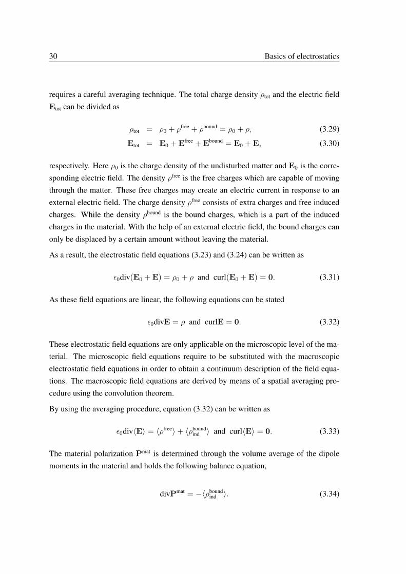
requires a careful averaging technique. The total charge density ρtot and the electric fieldEtot can be divided as
ρtot = ρ0 + ρfree + ρbound = ρ0 + ρ, (3.29)
Etot = E0 + Efree + Ebound = E0 + E, (3.30)
respectively. Here ρ0 is the charge density of the undisturbed matter and E0 is the corre-sponding electric field. The density ρfree is the free charges which are capable of movingthrough the matter. These free charges may create an electric current in response to anexternal electric field. The charge density ρfree consists of extra charges and free inducedcharges. While the density ρbound is the bound charges, which is a part of the inducedcharges in the material. With the help of an external electric field, the bound charges canonly be displaced by a certain amount without leaving the material.
As a result, the electrostatic field equations (3.23) and (3.24) can be written as
ε0div(E0 + E) = ρ0 + ρ and curl(E0 + E) = 0. (3.31)
As these field equations are linear, the following equations can be stated
ε0divE = ρ and curlE = 0. (3.32)
These electrostatic field equations are only applicable on the microscopic level of the ma-terial. The microscopic field equations require to be substituted with the macroscopicelectrostatic field equations in order to obtain a continuum description of the field equa-tions. The macroscopic field equations are derived by means of a spatial averaging pro-cedure using the convolution theorem.
By using the averaging procedure, equation (3.32) can be written as
ε0div〈E〉 = 〈ρfree〉+ 〈ρboundind 〉 and curl〈E〉 = 0. (3.33)
The material polarization Pmat is determined through the volume average of the dipolemoments in the material and holds the following balance equation,
divPmat = −〈ρboundind 〉. (3.34)
3.5 Electrostatics in matter 31
Equations (3.34) and (3.33) give
div (〈ε0E〉+ Pmat) = 〈ρfree〉. (3.35)
The macroscopic electrostatic field equations
divD = ρ and curlE = 0 (3.36)
are derived from (3.35) by using the definition of the electric displacement D = 〈ε0E〉+
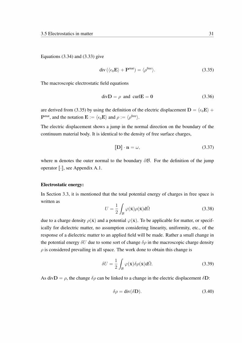
Pmat, and the notation E := 〈ε0E〉 and ρ := 〈ρfree〉.The electric displacement shows a jump in the normal direction on the boundary of thecontinuum material body. It is identical to the density of free surface charges,
JDK · n = ω, (3.37)
where n denotes the outer normal to the boundary ∂B. For the definition of the jumpoperator J·K, see Appendix A.1.
Electrostatic energy:
In Section 3.3, it is mentioned that the total potential energy of charges in free space iswritten as
U =1
2
∫
Bϕ(x)ρ(x)dΩ (3.38)
due to a charge density ρ(x) and a potential ϕ(x). To be applicable for matter, or specif-ically for dielectric matter, no assumption considering linearity, uniformity, etc., of theresponse of a dielectric matter to an applied field will be made. Rather a small change inthe potential energy δU due to some sort of change δρ in the macroscopic charge densityρ is considered prevailing in all space. The work done to obtain this change is
δU =1
2
∫
Bϕ(x)δρ(x)dΩ. (3.39)
As divD = ρ, the change δρ can be linked to a change in the electric displacement δD:
δρ = div(δD). (3.40)
32 Basics of electrostatics
In the following the total potential energy change can be written as
δU =
∫
BE · δDdΩ, (3.41)
where the electric field definition E = −∇ϕ is used and ρ(x) is considered as a localizedcharge distribution.
If the medium is assumed linear, then
E · δD =1
2δ(E ·D), (3.42)
and the change of total potential energy is
δU =1
2
∫
Bδ(E ·D)dΩ, (3.43)
and the total potential energy can be expressed as
U =1
2
∫
BE ·DdΩ. (3.44)
In a local form the electric energy density for matter is written as
W =1
2E ·D. (3.45)
Chapter 4
Theory of piezoelectric materials
This chapter provides a brief overview about the material theory of piezoelectric materi-als. The purpose of the theory of piezoelectric materials is to describe mathematically thematerial behaviour. This chapter includes field equations, material laws and configura-tional force theory of these materials. It also gives a numerical treatment of the standardboundary value problem (BVP) of piezoelectric materials as well as of configurationalforces. As piezoelectric materials exhibit an electro-mechanical coupling, the correspond-ing theories for both mechanical and electrical parts for matter are presented. Piezoelec-tric materials produce an internal electric field when they are strained. On the other hand,piezoelectric materials exhibit strain or stress when an external electric field is appliedto them. Here the field equations for both mechanical and electrical part are presentedseparately, and the coupling between the mechanical and electrical behavior of piezoelec-tric materials is obtained through the material laws. Readers are referred for a detailedtheoretical background of piezoelectric materials to Müller et al. [72], Schrade et al. [88],etc. For numerical treatment of BVP of piezoelectric materials see Allik and Hughes [3],Müller et al. [72], etc.
4.1 Field equations
We consider a piezoelectric body B which contains a domain wall and two domains. Thenormal vector nS to a domain wall S points from the sub-body B− into B+, for details see
34 Theory of piezoelectric materials
Figure 4.1. Neglecting the inertia term the Cauchy stress tensor σ fulfills the mechanicalequilibrium condition. The mechanical equilibrium has the form
divσ + f = 0 in B,JσKnS = 0 on S,
(4.1)
in the bulk considering the body force f and on the domain wall, respectively. See Ap-pendix A.1 or Müller et al. [72] for the definition of the jump operator J(·)K. The mechan-ical problem needs to be completed with suitable boundary conditions. Assigning eitherthe displacements u∗ on the boundary ∂Bu or the tractions t∗ on the boundary ∂Bt, onehas
u = u∗ on ∂Bu,σn = t∗ on ∂Bt.
(4.2)
The electric displacement D fulfills the electrostatic relation (Gauß law). In the presenceof volume charges q, the field equations in the bulk and on the domain wall are
div D− q = 0 in B,JDK·nS = 0 on S (charge free interfaces).
(4.3)
One can prescribe either the electric potential ϕ∗ or the surface chargeQ∗ on the boundary,
ϕ = ϕ∗ on ∂Bϕ,D · n = −Q∗ on ∂BQ.
(4.4)
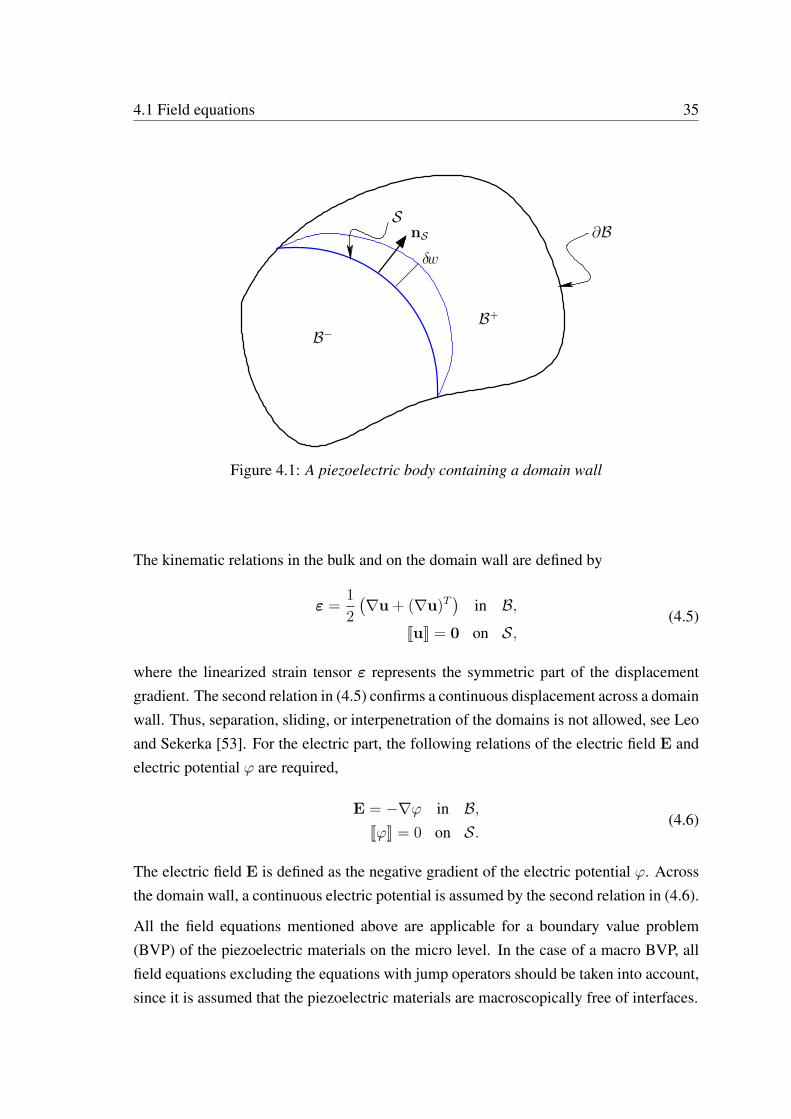
4.1 Field equations 35
B−
∂B
B+
S
δw
nS
Figure 4.1: A piezoelectric body containing a domain wall
The kinematic relations in the bulk and on the domain wall are defined by
ε =1
2
(∇u + (∇u)T
)in B,
JuK = 0 on S,(4.5)
where the linearized strain tensor ε represents the symmetric part of the displacementgradient. The second relation in (4.5) confirms a continuous displacement across a domainwall. Thus, separation, sliding, or interpenetration of the domains is not allowed, see Leoand Sekerka [53]. For the electric part, the following relations of the electric field E andelectric potential ϕ are required,
E = −∇ϕ in B,JϕK = 0 on S.
(4.6)
The electric field E is defined as the negative gradient of the electric potential ϕ. Acrossthe domain wall, a continuous electric potential is assumed by the second relation in (4.6).
All the field equations mentioned above are applicable for a boundary value problem(BVP) of the piezoelectric materials on the micro level. In the case of a macro BVP, allfield equations excluding the equations with jump operators should be taken into account,since it is assumed that the piezoelectric materials are macroscopically free of interfaces.
36 Theory of piezoelectric materials
4.2 Piezoelectric constitutive law
To complete the field equations in the previous sections for a certain material, constitutiverelations are needed, which relate the Cauchy stress tensor σ and the electric displace-ment vector D to the strain tensor ε and the electric field E. The material response ofa ferroelectric ceramic under small electric or mechanical loading may be described bya linear piezoelectric constitutive law. One can write the electric enthalpy function as athermodynamical potential,
H(ε,E) =1
2(ε− ε0):
[C(ε− ε0)
]− (ε− ε0): (bTE)− 1
2E·(A E)−P0 ·E, (4.7)
which comprises an elastic, an electric and a coupling part. Taking the partial derivativewith respect to ε and the negative of the partial derivative with respect to E, one obtainsthe Cauchy stress tensor σ and the electric displacement D via
σ =∂H
∂ε= C(ε− ε0)− bTE, (4.8)
D = −∂H∂E
= b(ε− ε0) + A E + P0, (4.9)
where C is the elastic tensor, b the piezoelectric tensor, A the dielectric tensor, ε0 theremanent strain, and P0 the spontaneous polarization.
4.3 Numerical implementation of piezoelectric materialsusing finite elements
In the previous sections, the theory of piezoelectric materials (BVP of piezoelectric mate-rials) was illustrated. For a piezoelectric body with simple geometry and simple domainstructure, the system of BVPs may be solved analytically. In the case of a piezoelec-tric body with complex geometry and complex domain structure, numerical methods areused to solve the BVPs. In the following section, a numerical treatment of the BVPsfor piezoelectric materials using finite element method will be presented. For a detaileddescription of the numerical methods of piezoelectric materials, the reader is referred toAllik and Hughes [3], Müller et al. [72], etc.
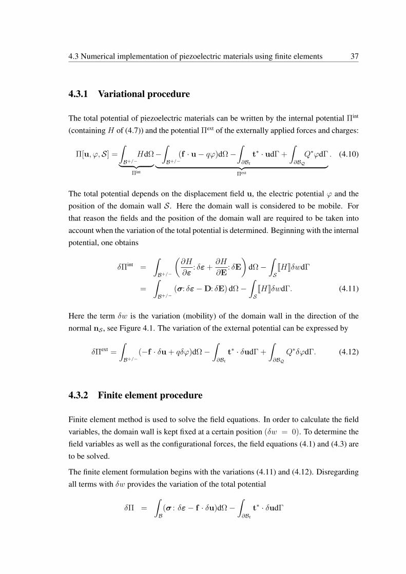
4.3 Numerical implementation of piezoelectric materials using finite elements 37
4.3.1 Variational procedure
The total potential of piezoelectric materials can be written by the internal potential Πint
(containing H of (4.7)) and the potential Πext of the externally applied forces and charges:
Π[u, ϕ,S] =
∫
B+/−HdΩ
︸ ︷︷ ︸Πint
−∫
B+/−(f · u− qϕ)dΩ−
∫
∂Btt∗ · udΓ +
∫
∂BQQ∗ϕdΓ
︸ ︷︷ ︸Πext
. (4.10)
The total potential depends on the displacement field u, the electric potential ϕ and theposition of the domain wall S. Here the domain wall is considered to be mobile. Forthat reason the fields and the position of the domain wall are required to be taken intoaccount when the variation of the total potential is determined. Beginning with the internalpotential, one obtains
δΠint =
∫
B+/−
(∂H
∂ε: δε+
∂H
∂E: δE
)dΩ−
∫
SJHKδwdΓ
=
∫
B+/−(σ: δε−D: δE) dΩ−
∫
SJHKδwdΓ. (4.11)
Here the term δw is the variation (mobility) of the domain wall in the direction of thenormal nS , see Figure 4.1. The variation of the external potential can be expressed by
δΠext =
∫
B+/−(−f · δu + qδϕ)dΩ−
∫
∂Btt∗ · δudΓ +
∫
∂BQQ∗δϕdΓ. (4.12)
4.3.2 Finite element procedure
Finite element method is used to solve the field equations. In order to calculate the fieldvariables, the domain wall is kept fixed at a certain position (δw = 0). To determine thefield variables as well as the configurational forces, the field equations (4.1) and (4.3) areto be solved.
The finite element formulation begins with the variations (4.11) and (4.12). Disregardingall terms with δw provides the variation of the total potential
δΠ =
∫
B(σ : δε− f · δu)dΩ−
∫
∂Btt∗ · δudΓ
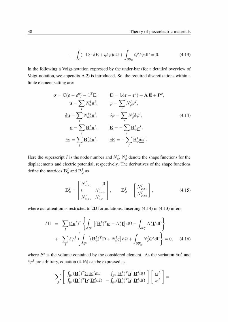
38 Theory of piezoelectric materials
+
∫
B(−D · δE + qδϕ)dΩ +
∫
∂BQQ∗δϕdΓ = 0. (4.13)
In the following a Voigt-notation expressed by the under-bar (for a detailed overview ofVoigt-notation, see appendix A.2) is introduced. So, the required discretizations within afinite element setting are:
σ = C(ε− ε0)− bTE, D = b(ε− ε0) + A E + P0,
u =∑
I
N Iuu
I , ϕ =∑
I
N Iϕϕ
I ,
δu =∑
I
N Iuδu
I , δϕ =∑
I
N Iϕδϕ
I , (4.14)
ε =∑
I
BIuu
I , E = −∑
I
BIϕϕ
I ,
δε =∑
I
BIuδu
I , δE = −∑
I
BIϕδϕ
I .
Here the superscript I is the node number and N Iu , N I
ϕ denote the shape functions for thedisplacements and electric potential, respectively. The derivatives of the shape functionsdefine the matrices BI
u and BIϕ as
BIu =
N Iu,x1
0
0 N Iu,x2
N Iu,x2
N Iu,x1
, BI
ϕ =
[N Iϕ,x1
N Iϕ,x2
], (4.15)
where our attention is restricted to 2D formulations. Inserting (4.14) in (4.13) infers
δΠ =∑
I
(δuI)T
∫
Be
[(BI
u)Tσ −N I
uf]
dΩ−∫
∂BetN Iut∗dΓ
+∑
I
δϕI
∫
Be
[(BI
ϕ)TD +N Iϕq]
dΩ +
∫
∂BeQN IϕQ∗dΓ
= 0, (4.16)
where Be is the volume contained by the considered element. As the variation δuI andδϕI are arbitrary, equation (4.16) can be expressed as
∑
J
[ ∫Be(B
Iu)TCBJ
udΩ∫Be(B
Iu)TbTBJ
ϕdΩ∫Be(B
Iϕ)TbTBJ
udΩ −∫Be(B
Iϕ)TbTBJ
ϕdΩ
][uJ
ϕJ
]=
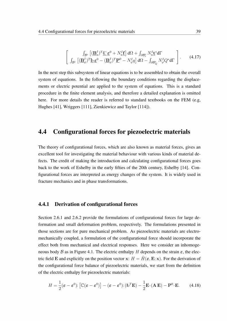
4.4 Configurational forces for piezoelectric materials 39
[ ∫Be[(BI
u)TC ε0 +N I
uf]
dΩ +∫∂Bet
N Iut∗dΓ
∫Be[(BI
ϕ)Tb ε0 − (BIϕ)TP0 −N I
ϕq]
dΩ−∫∂BeQ
N IϕQ∗dΓ
]. (4.17)
In the next step this subsystem of linear equations is to be assembled to obtain the overallsystem of equations. In the following the boundary conditions regarding the displace-ments or electric potential are applied to the system of equations. This is a standardprocedure in the finite element analysis, and therefore a detailed explanation is omittedhere. For more details the reader is referred to standard textbooks on the FEM (e.g,Hughes [41], Wriggers [111], Zienkiewicz and Taylor [114]).
4.4 Configurational forces for piezoelectric materials
The theory of configurational forces, which are also known as material forces, gives anexcellent tool for investigating the material behaviour with various kinds of material de-fects. The credit of making the introduction and calculating configurational forces goesback to the work of Eshelby in the early fifties of the 20th century, Eshelby [14]. Con-figurational forces are interpreted as energy changes of the system. It is widely used infracture mechanics and in phase transformations.
4.4.1 Derivation of configurational forces
Section 2.6.1 and 2.6.2 provide the formulations of configurational forces for large de-formation and small deformation problem, respectively. The formulations presented inthose sections are for pure mechanical problem. As piezoelectric materials are electro-mechanically coupled, a formulation of the configurational force should incorporate theeffect both from mechanical and electrical responses. Here we consider an inhomoge-neous body B as in Figure 4.1. The electric enthalpy H depends on the strain ε, the elec-tric field E and explicitly on the position vector x: H = H(ε,E; x). For the derivation ofthe configurational force balance of piezoelectric materials, we start from the definitionof the electric enthalpy for piezoelectric materials:
H =1
2(ε− ε0):
[C(ε− ε0)
]− (ε− ε0): (bTE)− 1
2E·(A E)−P0 ·E. (4.18)
40 Theory of piezoelectric materials
This implies for fixed spontaneous strain and fixed spontaneous polarization the followingrate form
H = ε:[C(ε− ε0)
]− ε: (bTE)− b(ε− ε0) ·E− (A E)·E−P0 ·E
= ε:[C(ε− ε0)− bTE
]−[b(ε− ε0) + A E + P0
]· E
= σ: ε−D · E. (4.19)
By using the definition of the strain tensor ε =1
2(∇u + (∇u)T ) and the electric
field E = −∇ϕ, equation (4.19) can be written as
H = σ : ∇u︸ ︷︷ ︸Hm
+ D · ∇ϕ︸ ︷︷ ︸He
. (4.20)
Using the product rule, equation (4.20) can be rewritten as
H = (σ : ∇u)· − σ : ∇u + (D · ∇ϕ)· − D · ∇ϕ. (4.21)
Then the gradient of (4.21) is given by
∇H = ∇(σ : ∇u)· −∇(σ : ∇u) +∇(D · ∇ϕ)· −∇(D · ∇ϕ). (4.22)
Using the identities
∇(σ : ∇u) = ∇σ : ∇u + div((∇u)Tσ
)− (∇u)Tdivσ,
∇(D · ∇ϕ) = ∇D∇ϕ+ div(∇ϕ⊗D)−∇ϕdivD,
equation (4.22) can be reformulated as
∇H − div((∇u)Tσ
)·+
((∇u)Tdivσ
)·+∇(σ : ∇u)− (∇σ : ∇u)·
−div(∇ϕ⊗D)· + (∇ϕdivD)· +∇(D · ∇ϕ)− (∇D∇ϕ)· = 0. (4.23)
Integrating equation (4.23) with respect to time t and using the mechanical equilibriumcondition divσ+ f = 0 as well as the electrostatic balance condition divD− q = 0 yields
divΣ− (∇u)T f + (∇ϕ)q
4.4 Configurational forces for piezoelectric materials 41
+
∫ t
0
(∇(σ : ∇u)− (∇σ : ∇u)· +∇(D · ∇ϕ)− (∇D∇ϕ)·
)dτ = 0, (4.24)
whereΣ = H 1− (∇u)Tσ −∇ϕ⊗D (4.25)
is introduced as the electro-mechanical Eshelby stress tensor.
Rewriting the time integrals in (4.24) for the mechanical and electrical part (subscript mand e for mechanical and electrical, respectively) as
∫ t
0
(σ : ∇∇u−∇σ :∇u) dτ =
∫ t
0
((σ :∇∇u)· − σ :∇∇u−∇σ :∇u) dτ
= σ :∇∇u−∫ t
0
(σ :∇∇u +∇σ :∇u︸ ︷︷ ︸∇Hm
)dτ, (4.26)
and∫ t
0
(∇(∇ϕ)D−∇D∇ϕ
)dτ =
∫ t
0
((∇(∇ϕ)D)· −∇(∇ϕ)D−∇D∇ϕ) dτ
= ∇(∇ϕ)D−∫ t
0
(∇(∇ϕ)D +∇D∇ϕ︸ ︷︷ ︸∇He
)dτ, (4.27)
the configurational force balance for piezoelectric materials
divΣ + g = 0,
with g = −(∇u)T f + (∇ϕ)q + σ : ∇∇u−∇(∇ϕ)D− (∇Hm +∇He︸ ︷︷ ︸∇H
) (4.28)
is obtained. The term g is called configurational volume force. The gradient of the electricenthalpy H = H(ε,E; x) can be demonstrated as
∇H =∂H
∂ε︸︷︷︸σ
: ∇∇u +∇(∇ϕ)∂H
∂E︸︷︷︸−D
+∂H
∂x
∣∣∣∣∣expl.
, (4.29)
42 Theory of piezoelectric materials
with the notation expl. for the explicit derivative with respect to position x. Therefore,the local configurational force g can be compactly summarized as
g = −(∇u)T f + (∇ϕ)q − ∂H
∂x
∣∣∣∣∣expl.
. (4.30)
From this it can be concluded that all of the following can cause a configurational force:1) a physical body force f ; 2) a volume charge density q; 3) an inhomogeneity in thematerial. As a consequence, the Eshelby stress tensor Σ is not a divergence free quantityin these cases. According to Kienzler & Herrmann [48] this gives the fact that the Eshelbystress tensor is not a conserved quantity.
4.4.2 Numerical implementation of configurational forces using fi-nite elements
To obtain nodal configurational forces based on a FE calculation, the balance equation in(4.28) is discretized in a consistent way by approximating other field equations. Begin-ning with the weak form of (4.28) by a test function η,
∫
B(divΣ + g) · ηdΩ = 0, (4.31)
and by using integration by parts, equation (4.31) can be written as
∫
∂B(Σn) · ηdΓ−
∫
BΣ : ∇ηdΩ +
∫
Bg · ηdΩ = 0, (4.32)
where n is the unit normal vector to the boundary. It is assumed that the test function ηdisappears on the boundary ∂B, hence the first integral in (4.32) will be zero. This as-sumption leads to a stationary boundary, which does not change its position x.
In this thesis our attention is kept restricted to a 2D formulation (plane strain), but the ex-tension to 3D is straightforward and will not be described in detail here. The test functionin (4.32) is approximated in each element Be by node values ηI and shape functions N I :
η =∑
I
N IηI , where η = [η1 η2]T and ηI =[ηI1 η
I2
]T. (4.33)
4.4 Configurational forces for piezoelectric materials 43
By formulating the gradient of the test function and the electro-mechanical Eshelby stresstensor as in the following matrix notation
∇η = [η1,1 η2,2 η1,2 η2,1]T =∑
I
DIηI , where DI =
N I,x1
0
0 N I,x2
N I,x2
0
0 N I,x1
,
Σ = [Σ11 Σ22 Σ12 Σ21]T and g = [g1 g2]T , (4.34)
one has the element-wise discretization of (4.32)
∑
I
ηIT ·[−∫
BeDIT ·ΣdΩ +
∫
BeN IgdΩ
]= 0. (4.35)
It needs to be stated that the Voigt-notation for symmetric tensors cannot be considered,since the Eshelby stress tensor is generally not symmetric, see (4.25). The Eshelby stresstensor Σ shows the symmetry only if the material is isotropic. As equation (4.35) is to besatisfied for arbitrary nodal values ηI , the term within the square brackets must disappear.This obviously yields the discrete configurational forces
GIe =
GIe1
GIe2
=
∫
BeN IgIdΩ =
∫
BeDIT ·ΣdΩ
=
∫
Be
N I,x1
Σ11 +N I,x2
Σ12
N I,x1
Σ21 +N I,x2
Σ22
dΩ. (4.36)
The configurational forces GIe regarding all ne elements adjacent to node K are then
assembled to a total configurational force
GK =ne⋃
e=1
GIe. (4.37)
This does not give a new boundary value problem, as the nodal values GK can be deter-mined from the quantities that are already computed (strain, stress, deformation measures,electric field, electric displacement and electric potential measures) in the solution of thedisplacement fields and the electric potentials. The determination of the discrete configu-rational forces is therefore considered as a post-processing step.

44 Theory of piezoelectric materials
Chapter 5
Material homogenization in a smallstrain framework using configurationalforce theory
In this chapter a homogenization technique for a pure mechanical problem is describedto determine the homogenized mechanical quantities. Special attention is given to thehomogenization of the Eshelby stress tensor. Among the homogenization techniques, theFE2-based homogenization is computationally efficient. This homogenization is a two-scale homogenization, in which two boundary value problems (BVPs) are solved: one onthe macro level, and the other on the micro level. On the macro level no constitutive lawis prescribed, but a boundary value problem on the micro level is used to determine thehomogenized material response. In order to obtain representative numerical results on themacro level, or to capture the effect of micro inhomogeneities on the macro problem, it isnecessary to attach a micro domain to each macro Gauß point. This micro domain shouldcontain enough microstructural features of the material. Therefore, it is usually calledrepresentative volume element (RVE), see Figure 5.1. In order to solve the micro BVP,admissible boundary conditions are required.
A literature review reveals that the macro strain tensor is used to define the boundaryconditions for the micro BVP in deformation driven homogenization. This gives con-sistent simulation results for the homogenized Cauchy stress tensor and the homogenizedmaterial parameters. However, the homogenization of the Eshelby stress tensor gives non-physical results for the macro configurational forces if a deformation driven homogeniza-
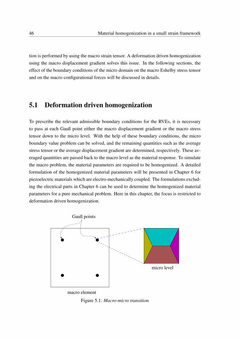
46 Material homogenization in a small strain framework
tion is performed by using the macro strain tensor. A deformation driven homogenizationusing the macro displacement gradient solves this issue. In the following sections, theeffect of the boundary conditions of the micro domain on the macro Eshelby stress tensorand on the macro configurational forces will be discussed in details.
5.1 Deformation driven homogenization
To prescribe the relevant admissible boundary conditions for the RVEs, it is necessaryto pass at each Gauß point either the macro displacement gradient or the macro stresstensor down to the micro level. With the help of these boundary conditions, the microboundary value problem can be solved, and the remaining quantities such as the averagestress tensor or the average displacement gradient are determined, respectively. These av-eraged quantities are passed back to the macro level as the material response. To simulatethe macro problem, the material parameters are required to be homogenized. A detailedformulation of the homogenized material parameters will be presented in Chapter 6 forpiezoelectric materials which are electro-mechanically coupled. The formulations exclud-ing the electrical parts in Chapter 6 can be used to determine the homogenized materialparameters for a pure mechanical problem. Here in this chapter, the focus is restricted todeformation driven homogenization.
Gauß points
macro element
micro level
Figure 5.1: Macro-micro transition
5.1 Deformation driven homogenization 47
In the following the macro or averaged quantities are denoted by the symbols with anover-bar, while the micro quantities remain unmarked. In the absence of body forces, thetransition between the macro and the micro quantities is given by
ε =1
V
∫
Bmic
ε dΩ =1
V
∫
∂Bmic
sym(u⊗n) dΓ, σ =1
V
∫
Bmic
σ dΩ =1
V
∫
∂Bmic
sym(t⊗x) dΓ. (5.1)
A comprehensive proof of the connection between the macro and the micro quantities hasbeen discussed in Schröder [91].
5.1.1 Determination of the admissible boundary conditions for themicro BVP
To have a consistent transition between the macro and the micro quantities, it is essentialto satisfy an energy criterion which is the so called Hill-Mandel condition. The Hill-Mandel condition for a pure mechanical problem is defined by
σ : ε =1
V
∫
Bmic
σ : ε dΩ. (5.2)
The condition assumes that the mechanical power on the macro level is equivalent to thevolume average of the mechanical power on the micro level. By introducing Pm, theHill-Mandel condition (5.2) can be formulated as
Pm =1
V
∫
Bmic
σ : ε dΩ− σ : ε. (5.3)
The volume integral in (5.3) can be converted to surface or boundary integral with theGauß formula:
1
V
∫
Bmic
σ : ε dΩ =1
V
∫
∂Bmic
t · u dΓ. (5.4)
By adding and subtracting the term σ : ε to the right hand side (RHS) of (5.3) and byusing (5.4), Pm can be written as
Pm =1
V
∫
∂Bmic
t ·u dΓ− σ : ε− σ : ε+ σ : ε. (5.5)
48 Material homogenization in a small strain framework
By using the definitions of the average quantities or the boundary integral on the microlevel, the mechanical power on the macro level σ : ε can be expressed in three differentways:
σ : ε = σ :1
V
∫
∂Bmic
sym[u⊗ n]dΓ =1
V
∫
∂Bmic
(σn) · udΓ,
σ : ε = σ : ∇u
=1
V
∫
∂Bmic
sym[t⊗ x] dΓ: ∇u =1
V
∫
∂Bmic
t ·(∇u x) dΓ,
σ : ε = σ : ∇u
= (σ1
V
∫
∂Bmic
n⊗ x dΓ): ∇u =1
V
∫
∂Bmic
(σn) ·(∇u x) dΓ
. (5.6)
Inserting the different expressions of σ : ε into the right hand side of (5.5) and doingrearrangements, the following equation is deduced:
Pm =1
V
∫
∂Bmic
[t·u− (σn) ·u− t ·(∇u x) + (σn) ·(∇u x)
]dΓ
=1
V
∫
∂Bmic
((t− σn) · (u− ∇u x)) dΓ. (5.7)
As Pm = 0, one of the two terms in the multiplication under the boundary integral in (5.7)must be zero. Thus, from equation (5.7) two types of mechanical boundary conditions forthe micro boundary value problem (BVP) are deduced,
t = σn or u = ∇u x on ∂Bmic. (5.8)
Another possible mechanical boundary condition for the micro scale problem is calledperiodic boundary condition. This boundary condition allows a fluctuation of u, i.e.
u = ∇u x + ˙w ⇒ ∇u = ∇u +∇ ˙w, (5.9)
where w denotes the fluctuation of the displacement field at the micro scale relative to thehomogeneous term ∇u x. Suppose that the boundary of the representative volume ele-
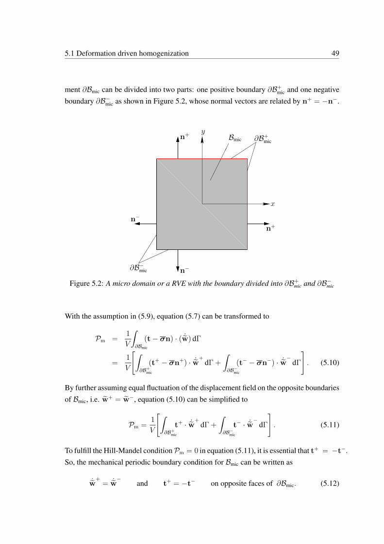
5.1 Deformation driven homogenization 49
ment ∂Bmic can be divided into two parts: one positive boundary ∂B+mic and one negative
boundary ∂B−mic as shown in Figure 5.2, whose normal vectors are related by n+ = −n−.
∂B+mic
∂B−mic
n+
n−
n−
n+
x
y
Bmic
Figure 5.2: A micro domain or a RVE with the boundary divided into ∂B+mic and ∂B−mic
With the assumption in (5.9), equation (5.7) can be transformed to
Pm =1
V
∫
∂Bmic
(t− σn) · ( ˙w) dΓ
=1
V
[∫
∂B+mic
(t+ − σn+) · ˙w+
dΓ +
∫
∂B−mic
(t− − σn−) · ˙w−
dΓ
]. (5.10)
By further assuming equal fluctuation of the displacement field on the opposite boundariesof Bmic, i.e. w+ = w−, equation (5.10) can be simplified to
Pm =1
V
[∫
∂B+mic
t+ · ˙w+
dΓ +
∫
∂B−mic
t− · ˙w−
dΓ
]. (5.11)
To fulfill the Hill-Mandel conditionPm = 0 in equation (5.11), it is essential that t+ = −t−.So, the mechanical periodic boundary condition for Bmic can be written as
˙w+
= ˙w−
and t+ = −t− on opposite faces of ∂Bmic. (5.12)
50 Material homogenization in a small strain framework
5.1.2 Mechanical power incorporating Eshelby stress tensor
In Section 5.1.1 the Hill-Mandel condition is written either in terms of the Cauchy stresstensor σ and strain tensor ε or the Cauchy stress tensor σ and the displacement gradient∇u. To investigate the consistency of the macro Eshelby stress tensor and the macro con-figurational forces, the Hill-Mandel condition has to be expressed by the Eshelby stresstensor. In order to obtain the Hill-Mandel condition, the relation between the mechanicalpower and the Eshelby stress tensor needs to be established. The mechanical power in asmall strain setting along with a linear elastic material can be written as
W = σ : ∇u = σ1 : ∇u = (∇u)T σ : 1
=[(
(∇u)T σ)·− (∇u)T σ
]: 1
=[(W1−Σ)· − (∇u)T σ
]: 1, as Σ = W1− (∇u)T σ
=[W1− Σ− (∇u)T σ
]: 1
= W1 : 1− Σ : 1− (∇u)T σ : 1
= 3W − Σ : 1− σ : ∇u, as 1 : 1 = 3
= 3W − Σ : 1− W , as W = σ : ∇u = σ : ∇u
⇒ W = 2W − Σ : 1
⇒ W = Σ : 1 = trΣ, (5.13)
in which W is the strain energy density and 1 is the second order unit tensor.
So, the mechanical power of the small strain problem with a linear material law can beexpressed in terms of the Eshelby stress tensor Σ as Σ : 1.
Thus, the Hill-Mandel condition incorporating the Eshelby stress tensor reads
ΣM : 1 =1
V
∫
Bmic
Σ : 1dΩ, (5.14)
where the subscript ‘M’ stands for macro or homogenized quantities.
The macro or homogenized Eshelby stress tensor in a small strain setting can be deter-mined in two different ways: either by using homogenized mechanical quantities (stresstensor and displacement gradient), or by performing a volume average of the Eshelbystress tensor on the micro level. More details on this issue are given in Section 5.2.
5.1 Deformation driven homogenization 51
Equation (5.14) can be rewritten as
ΣM : 1 = Σ : 1
= σ : ∇u, as W = Σ : 1 = σ : ∇u
= σ : ∇u, (Hill-Mandel condition in (5.2)). (5.15)
5.1.3 Boundary conditions of the micro BVP for pure mechanicalproblem
At this point of the derivation, it is possible to determine the displacement BC or theperiodic BC for the micro BVP by using the macro displacement gradient ∇u, or byusing the macro strain tensor ε.
Macro displacement gradient driven boundary conditions:
The displacement or Dirichlet BC is
u = ∇u x on ∂Bmic, (5.16)
and the corresponding micro displacement gradient on the boundary of the micro speci-men is
∇u = ∇u on ∂Bmic. (5.17)
The periodic BC isu = ∇u x + w on ∂Bmic, (5.18)
and the corresponding micro displacement gradient on the boundary of the micro speci-men is
∇u = ∇u +∇w on ∂Bmic. (5.19)
Macro strain driven boundary conditions:
The displacement or Dirichlet BC is
u = εx on ∂Bmic, (5.20)
52 Material homogenization in a small strain framework
and the corresponding micro displacement gradient on the boundary of the micro speci-men is
∇u = ε. (5.21)
The periodic BC isu = εx + w on ∂Bmic, (5.22)
and the corresponding micro displacement gradient on the boundary of the micro speci-men is
∇u = ε+∇w. (5.23)
5.2 Homogenization of the Eshelby stress tensor
In order to capture the effects of the micro inhomogeneities on the macro Eshelby stresstensor and macro configurational forces, it is essential to homogenize the Eshelby stresstensor. In the case of a large deformation problem, there are three possible different pro-cedures to homogenize the Eshelby stress tensor. The detailed formulation is describedby Ricker et al. [84]. In a small deformation setting along with linear material behavior,there are two possible procedures to homogenize the Eshelby stress tensor. In the firstprocedure, the homogenized Eshelby stress tensor is determined from homogenized me-chanical quantities, and in the second procedure, the homogenized Eshelby stress tensoris determined by performing the volume average of the Eshelby stress tensor on the microlevel.
5.2.1 Eshelby stress tensor from homogenized quantities
Here the homogenized or macro Eshelby stress is determined by using averaged or macroquantities as
ΣM = WM1− (∇uM)TσM
= W1− (∇u)Tσ, (5.24)
where W is the strain energy density.
5.2 Homogenization of the Eshelby stress tensor 53
5.2.1.1 Homogenized quantities using macro displacement gradient driven microboundary conditions
Here the formulation for periodic boundary conditions will be discussed first, and then theresults for Dirichlet boundary conditions can easily be obtained by omitting the fluctuationterm. By using the averaging definition of the mechanical quantities and considering theabsence of body force, equation (5.24) can be written as
ΣM =1
V
∫
Bmic
W1 dΩ− (∇u)T1
V
∫
Bmic
σ dΩ
=1
V
∫
Bmic
W1 dΩ− 1
V
∫
Bmic
(∇u)Tσ dΩ
=1
V
∫
Bmic
W1 dΩ− 1
V
∫
Bmic
(∇u−∇w)Tσ dΩ
=1
V
∫
Bmic
(W1− (∇u)Tσ) dΩ +1
V
∫
Bmic
(∇w)Tσ dΩ
=1
V
∫
Bmic
Σ dΩ +1
V
∫
Bmic
(∇w)Tσ dΩ
= Σ +1
V
∫
Bmic
(∇w)Tσ dΩ. (5.25)
The relation between the macro Eshelby stress tensor and the volume average of the Es-helby stress tensor is
ΣM = Σ +1
V
∫
Bmic
(∇w)Tσ dΩ. (5.26)
In the case of Dirichlet BC for the micro problem, ∇w = 0, which leads to ΣM = Σ.The macro Eshelby stress tensor is equivalent to the volume average of the Eshelby stresstensor.
The Hill-Mandel condition reads
ΣM : 1 = (Σ +1
V
∫
Bmic
(∇w)Tσ dΩ): 1
= Σ : 1 +1
V
∫
Bmic
[(∇w)Tσ
]: 1 dΩ
= Σ : 1 +1
V
∫
Bmic
σ : ∇w dΩ
= Σ : 1 +1
V
∫
Bmic
σ : ∇w dΩ. (5.27)
54 Material homogenization in a small strain framework
In the case of Dirichlet or displacement type BC, ∇w = 0, which infers ΣM : 1 = Σ : 1.So, the Hill-Mandel condition is satisfied.
5.2.1.2 Homogenized quantities using macro strain driven micro boundary condi-tions
Again by using the averaging definition on the mechanical quantities, equation (5.24) canbe written as
ΣM =1
V
∫
Bmic
W1 dΩ− (∇uM)T1
V
∫
Bmic
σ dΩ
=1
V
∫
Bmic
W1 dΩ− 1
V
∫
Bmic
(∇u)Tσ dΩ
=1
V
∫
Bmic
W1 dΩ− 1
V
∫
Bmic
(ε+ ω)Tσ dΩ (where ω =1
2
(∇u− (∇u)T
))
=1
V
∫
Bmic
W1 dΩ− 1
V
∫
Bmic
(∇u + ω −∇w)Tσ dΩ
=1
V
∫
Bmic
(W1− (∇u)Tσ) dΩ− 1
V
∫
Bmic
ωTσ dΩ +1
V
∫
Bmic
(∇w)Tσ dΩ
=1
V
∫
Bmic
Σ dΩ− 1
V
∫
Bmic
ωTσ dΩ +1
V
∫
Bmic
(∇w)Tσ dΩ
= Σ− 1
V
∫
Bmic
ωTσ dΩ +1
V
∫
Bmic
(∇w)Tσ dΩ. (5.28)
The relation between the macro Eshelby stress tensor and the volume average of the Es-helby stress tensor is
ΣM = Σ− 1
V
∫
Bmic
ωTσ dΩ +1
V
∫
Bmic
(∇w)Tσ dΩ. (5.29)
In the case of Dirichlet BC for the micro problem, ∇w = 0, which leads to ΣM =
Σ − 1V
∫BmicωTσ dΩ. The macro Eshelby stress tensor is not equivalent to the volume
average of the Eshelby stress tensor.
The Hill-Mandel condition reads
ΣM : 1 = (Σ− 1
V
∫
Bmic
ωTσ dΩ +1
V
∫
Bmic
(∇w)Tσ dΩ): 1
= Σ : 1− 1
V
∫
Bmic
[ωTσ
]: 1 dΩ +
1
V
∫
Bmic
[(∇w)Tσ
]: 1 dΩ
5.2 Homogenization of the Eshelby stress tensor 55
= Σ : 1 +1
V
∫
Bmic
σ : ∇w dΩ, as[ωTσ
]: 1 = 0
= Σ : 1 +1
V
∫
Bmic
σ : ∇w dΩ. (5.30)
In the case of Dirichlet or displacement type BC, ∇w = 0, this infers ΣM : 1 = Σ : 1.So, the Hill-Mandel condition is satisfied.
5.2.2 Macro Eshelby stress tensor as the volume average of microEshelby stress tensor
Here the homogenized or macro Eshelby stress tensor is determined by taking the volumeaverage of the Eshelby stress tensor on the micro level. The macro Eshelby stress tensoris defined as
ΣM = Σ =1
V
∫
Bmic
Σ dΩ. (5.31)
For the convenience of the formulations in the following section, index notation has beenused. With index notation, equation (5.31) can be written as
(ΣM)ij = Σij =1
V
∫
Bmic
Σij dΩ. (5.32)
The Hill-Mandel condition is easily satisfied in the following way,
ΣM : 1 = Σ : 1 = (1
V
∫
Bmic
Σ dΩ): 1 =1
V
∫
Bmic
(Σ : 1) dΩ = Σ : 1. (5.33)
It can be concluded that the Hill-Mandel condition is satisfied if the macro Eshelby stresstensor is determined by averaging the Eshelby stress tensor on the micro level. Thisprocedure is independent of the micro boundary conditions. This means that the Hill-Mandel condition is fulfilled for the micro boundary conditions determined either by usingthe macro displacement gradient or by using the macro strain tensor.
56 Material homogenization in a small strain framework
5.3 Balance of the homogenized configurational forces
In this section the balance of macro configurational forces is studied. As the homogenizedEshelby stress tensor determined by averaging the micro Eshelby stress tensor satisfies theHill-Mandel condition, this macro Eshelby stress tensor will be considered for the balancelaw.
5.3.1 Macro displacement gradient based deformation of the microdomain
The micro domain is deformed according to the macro displacement gradient. Both typesof micro boundary conditions, Dirichlet and periodic boundary conditions, are used toperform the homogenization process. Taking the divergence of both sides of equation(5.32) leads to
Σij,j =1
V
∫
Bmic
Σij,j dΩ
=1
V
∫
∂Bmic
Σijnj dΓ (according to divergence theorem). (5.34)
Mathematical manipulations in equation (5.34) gives (see Appendix A.3.1)
Σij,j = W,i−uk,ijσkj= 0 (as W,i−uk,ijσkj = gi = 0). (5.35)
In this case there are no unphysical volume configurational forces on the macro level.
5.3.2 Macro strain based deformation of the micro domain
Here the micro domain is deformed according to the macro strain. Similarly, by tak-ing the divergence of both sides of equation (5.32) and mathematical manipulation (seeAppendix A.3.2) leads to
Σij,j =1
V
∫
Bmic
Σij,j dΩ
5.4 Numerical results and analyses 57
= ωki,j1
V
∫
Bmic
σkj dΩ
= ωki,jσkj. (5.36)
If the macro strain tensor is used to determine the boundary conditions on the microlevel, there are unphysical volume configurational forces on the macro level as in equation(5.36), gi = −ωki,jσkj. This phenomenon is also seen in the numerical results of thehomogenization for a small strain problem.
5.4 Numerical results and analyses
In this chapter the main focus is to establish a numerical technique which is capable ofcapturing the effect of micro inhomogeneities in the elastic material on the macro re-sponses. Here the configurational forces at the crack tip of the macro domain are cal-culated to check the homogenization of configurational forces. The aim is to figure outthe influence of the underlying microstructure on the configurational force at the cracktip of a macro specimen. In a real life problem, the underlying microstructures contain-ing interfaces, grains, grain boundaries, micro defects, etc. are very complex in nature.Capturing the influences of the whole scenario of the underlying microstructures is a com-putationally expensive task or in some cases impossible. To understand the characteristicbehaviour of the microstructures, it is sufficient to restrict attention to simplified microdomains with different orientations of the interfaces, micro cracks and grains.
5.4.1 Macro geometry and material parameters
A 4 mm×4 mm macro specimen with a sharp crack (see Figure 5.3) is simulated to de-termine the configurational forces at the crack tip with different micro domains at everyGauß point of the macro domain. The length of the crack is 2 mm and the width of thecrack at the opening is 0.1 mm. In all simulations the bottom boundary of the macrodomain remains fixed and the top boundary is displaced by 0.1 mm.
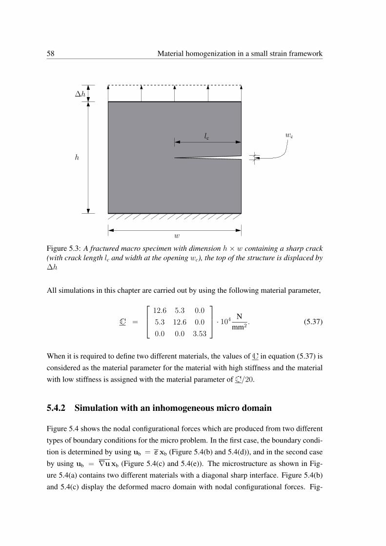
58 Material homogenization in a small strain framework
w
h
∆h
lc wc
Figure 5.3: A fractured macro specimen with dimension h × w containing a sharp crack(with crack length lc and width at the opening wc), the top of the structure is displaced by∆h
All simulations in this chapter are carried out by using the following material parameter,
C =
12.6 5.3 0.0
5.3 12.6 0.0
0.0 0.0 3.53
· 104 N
mm2. (5.37)
When it is required to define two different materials, the values of C in equation (5.37) isconsidered as the material parameter for the material with high stiffness and the materialwith low stiffness is assigned with the material parameter of C/20.
5.4.2 Simulation with an inhomogeneous micro domain
Figure 5.4 shows the nodal configurational forces which are produced from two differenttypes of boundary conditions for the micro problem. In the first case, the boundary condi-tion is determined by using ub = εxb (Figure 5.4(b) and 5.4(d)), and in the second caseby using ub = ∇u xb (Figure 5.4(c) and 5.4(e)). The microstructure as shown in Fig-ure 5.4(a) contains two different materials with a diagonal sharp interface. Figure 5.4(b)and 5.4(c) display the deformed macro domain with nodal configurational forces. Fig-
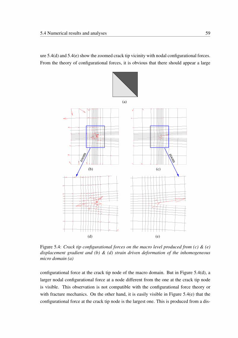
5.4 Numerical results and analyses 59
ure 5.4(d) and 5.4(e) show the zoomed crack tip vicinity with nodal configurational forces.From the theory of configurational forces, it is obvious that there should appear a large
(a)
(b) (c)
(d) (e)
zoom
AAAAAAAAU
zoom
Figure 5.4: Crack tip configurational forces on the macro level produced from (c) & (e)displacement gradient and (b) & (d) strain driven deformation of the inhomogeneousmicro domain (a)
configurational force at the crack tip node of the macro domain. But in Figure 5.4(d), alarger nodal configurational force at a node different from the one at the crack tip nodeis visible. This observation is not compatible with the configurational force theory orwith fracture mechanics. On the other hand, it is easily visible in Figure 5.4(e) that theconfigurational force at the crack tip node is the largest one. This is produced from a dis-
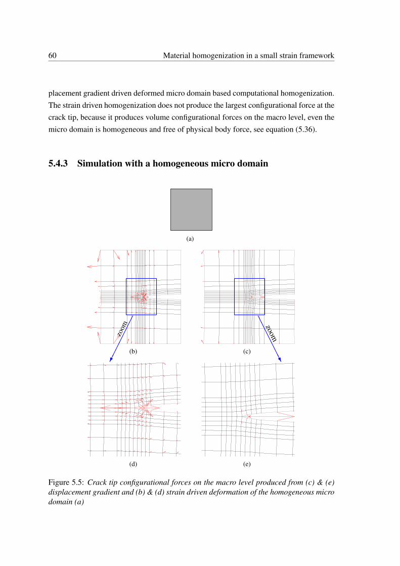
60 Material homogenization in a small strain framework
placement gradient driven deformed micro domain based computational homogenization.The strain driven homogenization does not produce the largest configurational force at thecrack tip, because it produces volume configurational forces on the macro level, even themicro domain is homogeneous and free of physical body force, see equation (5.36).
5.4.3 Simulation with a homogeneous micro domain
(a)
(b) (c)
(d) (e)
zoom
AAAAAAAU
zoom
Figure 5.5: Crack tip configurational forces on the macro level produced from (c) & (e)displacement gradient and (b) & (d) strain driven deformation of the homogeneous microdomain (a)
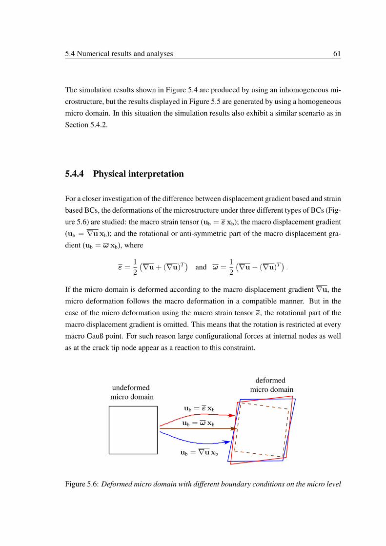
5.4 Numerical results and analyses 61
The simulation results shown in Figure 5.4 are produced by using an inhomogeneous mi-crostructure, but the results displayed in Figure 5.5 are generated by using a homogeneousmicro domain. In this situation the simulation results also exhibit a similar scenario as inSection 5.4.2.
5.4.4 Physical interpretation
For a closer investigation of the difference between displacement gradient based and strainbased BCs, the deformations of the microstructure under three different types of BCs (Fig-ure 5.6) are studied: the macro strain tensor (ub = εxb); the macro displacement gradient(ub = ∇u xb); and the rotational or anti-symmetric part of the macro displacement gra-dient (ub = ω xb), where
ε =1
2
(∇u + (∇u)T
)and ω =
1
2
(∇u− (∇u)T
).
If the micro domain is deformed according to the macro displacement gradient ∇u, themicro deformation follows the macro deformation in a compatible manner. But in thecase of the micro deformation using the macro strain tensor ε, the rotational part of themacro displacement gradient is omitted. This means that the rotation is restricted at everymacro Gauß point. For such reason large configurational forces at internal nodes as wellas at the crack tip node appear as a reaction to this constraint.
undeformed
micro domain
deformed
micro domain
ub = εxb
ub = ω xb
ub = ∇u xb
Figure 5.6: Deformed micro domain with different boundary conditions on the micro level
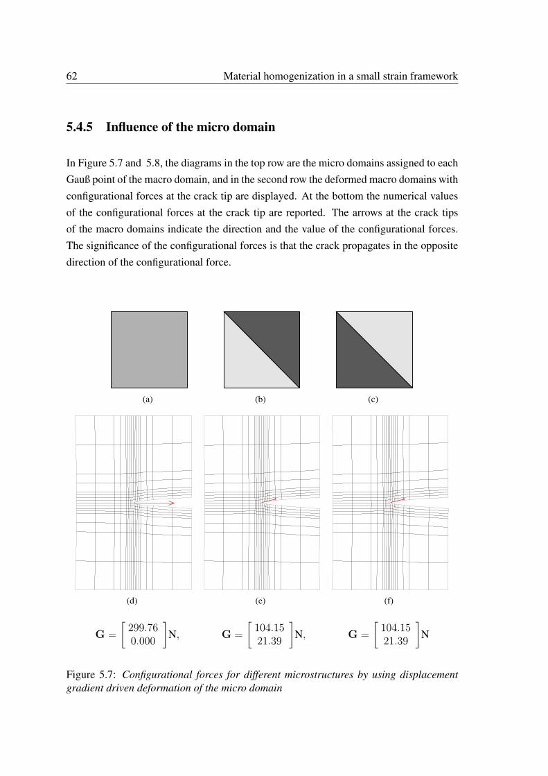
62 Material homogenization in a small strain framework
5.4.5 Influence of the micro domain
In Figure 5.7 and 5.8, the diagrams in the top row are the micro domains assigned to eachGauß point of the macro domain, and in the second row the deformed macro domains withconfigurational forces at the crack tip are displayed. At the bottom the numerical valuesof the configurational forces at the crack tip are reported. The arrows at the crack tipsof the macro domains indicate the direction and the value of the configurational forces.The significance of the configurational forces is that the crack propagates in the oppositedirection of the configurational force.
(a) (b) (c)
(d) (e) (f)
G =
[299.760.000
]N, G =
[104.1521.39
]N, G =
[104.1521.39
]N
Figure 5.7: Configurational forces for different microstructures by using displacementgradient driven deformation of the micro domain
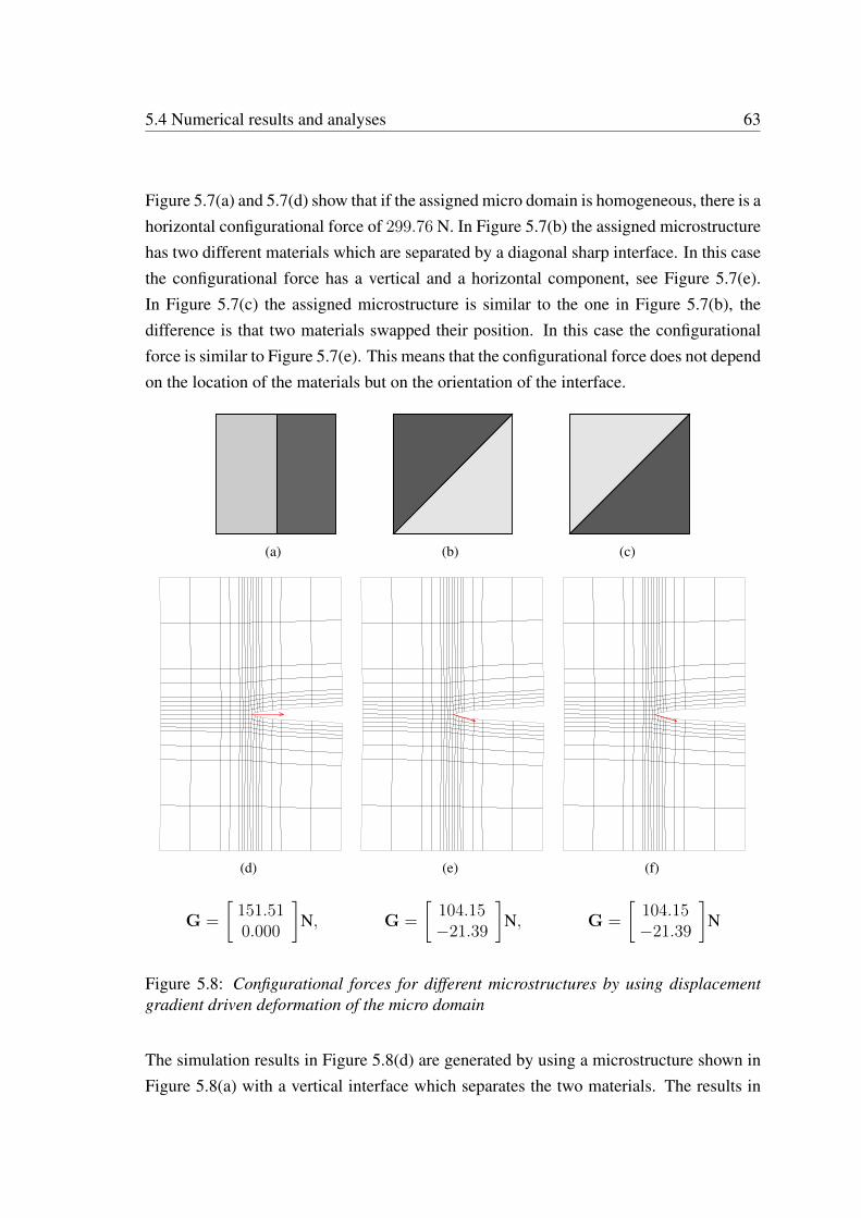
5.4 Numerical results and analyses 63
Figure 5.7(a) and 5.7(d) show that if the assigned micro domain is homogeneous, there is ahorizontal configurational force of 299.76 N. In Figure 5.7(b) the assigned microstructurehas two different materials which are separated by a diagonal sharp interface. In this casethe configurational force has a vertical and a horizontal component, see Figure 5.7(e).In Figure 5.7(c) the assigned microstructure is similar to the one in Figure 5.7(b), thedifference is that two materials swapped their position. In this case the configurationalforce is similar to Figure 5.7(e). This means that the configurational force does not dependon the location of the materials but on the orientation of the interface.
(a) (b) (c)
(d) (e) (f)
G =
[151.510.000
]N, G =
[104.15−21.39
]N, G =
[104.15−21.39
]N
Figure 5.8: Configurational forces for different microstructures by using displacementgradient driven deformation of the micro domain
The simulation results in Figure 5.8(d) are generated by using a microstructure shown inFigure 5.8(a) with a vertical interface which separates the two materials. The results in
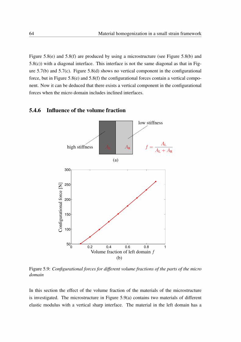
64 Material homogenization in a small strain framework
Figure 5.8(e) and 5.8(f) are produced by using a microstructure (see Figure 5.8(b) and5.8(c)) with a diagonal interface. This interface is not the same diagonal as that in Fig-ure 5.7(b) and 5.7(c). Figure 5.8(d) shows no vertical component in the configurationalforce, but in Figure 5.8(e) and 5.8(f) the configurational forces contain a vertical compo-nent. Now it can be deduced that there exists a vertical component in the configurationalforces when the micro domain includes inclined interfaces.
5.4.6 Influence of the volume fraction
(a)
Con
figur
atio
nalf
orce
[N]
Volume fraction of left domain f(b)
high stiffness
low stiffness
AL AR f =AL
AL + AR
Figure 5.9: Configurational forces for different volume fractions of the parts of the microdomain
In this section the effect of the volume fraction of the materials of the microstructureis investigated. The microstructure in Figure 5.9(a) contains two materials of differentelastic modulus with a vertical sharp interface. The material in the left domain has a
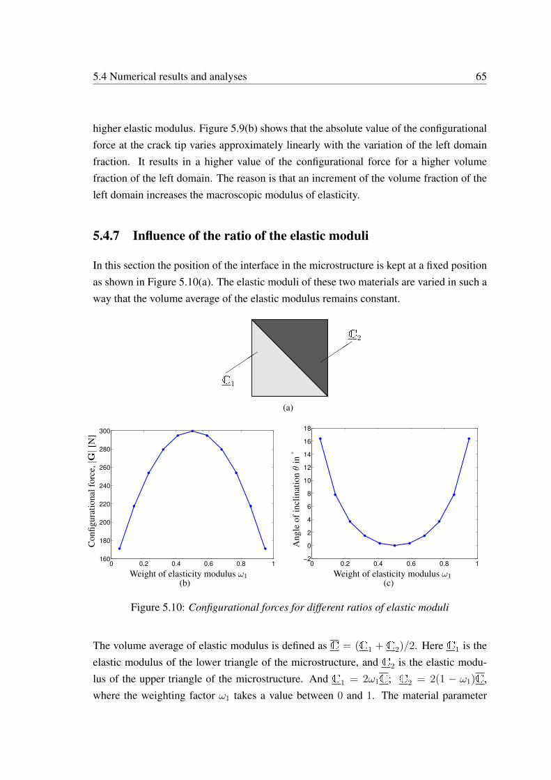
5.4 Numerical results and analyses 65
higher elastic modulus. Figure 5.9(b) shows that the absolute value of the configurationalforce at the crack tip varies approximately linearly with the variation of the left domainfraction. It results in a higher value of the configurational force for a higher volumefraction of the left domain. The reason is that an increment of the volume fraction of theleft domain increases the macroscopic modulus of elasticity.
5.4.7 Influence of the ratio of the elastic moduli
In this section the position of the interface in the microstructure is kept at a fixed positionas shown in Figure 5.10(a). The elastic moduli of these two materials are varied in such away that the volume average of the elastic modulus remains constant.
(a)
0 0.2 0.4 0.6 0.8 1160
180
200
220
240
260
280
300
Con
figur
atio
nalf
orce
,|G|[
N]
Weight of elasticity modulus ω1(b)
0 0.2 0.4 0.6 0.8 1−2
0
2
4
6
8
10
12
14
16
18
Ang
leof
incl
inat
ionθ
in°
Weight of elasticity modulus ω1(c)
C1
C2
Figure 5.10: Configurational forces for different ratios of elastic moduli
The volume average of elastic modulus is defined as C = (C1 + C2)/2. Here C1 is theelastic modulus of the lower triangle of the microstructure, and C2 is the elastic modu-lus of the upper triangle of the microstructure. And C1 = 2ω1C; C2 = 2(1 − ω1)C,where the weighting factor ω1 takes a value between 0 and 1. The material parameter
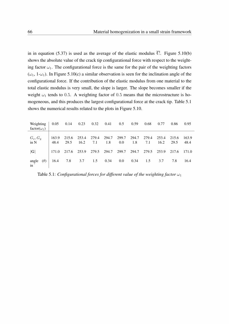
66 Material homogenization in a small strain framework
in in equation (5.37) is used as the average of the elastic modulus C. Figure 5.10(b)shows the absolute value of the crack tip configurational force with respect to the weight-ing factor ω1. The configurational force is the same for the pair of the weighting factors(ω1, 1-ω1). In Figure 5.10(c) a similar observation is seen for the inclination angle of theconfigurational force. If the contribution of the elastic modulus from one material to thetotal elastic modulus is very small, the slope is larger. The slope becomes smaller if theweight ω1 tends to 0.5. A weighting factor of 0.5 means that the microstructure is ho-mogeneous, and this produces the largest configurational force at the crack tip. Table 5.1shows the numerical results related to the plots in Figure 5.10.
Weightingfactor(ω1)
0.05 0.14 0.23 0.32 0.41 0.5 0.59 0.68 0.77 0.86 0.95
Gx, Gy 163.9 215.6 253.4 279.4 294.7 299.7 294.7 279.4 253.4 215.6 163.9in N 48.4 29.5 16.2 7.1 1.8 0.0 1.8 7.1 16.2 29.5 48.4
|G| 171.0 217.6 253.9 279.5 294.7 299.7 294.7 279.5 253.9 217.6 171.0
angle (θ)in °
16.4 7.8 3.7 1.5 0.34 0.0 0.34 1.5 3.7 7.8 16.4
Table 5.1: Configurational forces for different value of the weighting factor ω1
Chapter 6
Homogenization of piezoelectricmaterials
In this chapter the FE2-based homogenization technique of the mechanical and electri-cal quantities as well as the material parameters of piezoelectric materials is presented.An additional task in this chapter is to determine the homogenized configurational forcesfor microscopically inhomogeneous piezoelectric materials. Since piezoelectric materialsexhibit small deformations, all formulations in the previous chapter regarding the homog-enization of configurational forces will be taken into consideration. Following the conclu-sion obtained in Chapter 5, the macro displacement gradient driven boundary conditionson the micro domains will be used for the homogenization of the mechanical part of piezo-electric materials in order to obtain physically compatible configurational forces on themacro level. To prescribe the relevant admissible boundary conditions on the RVEs, oneneeds to pass at each Gauß point either the macro displacement gradient and the macroelectric field, or the macro stress tensor and the macro electric displacement down to themicro level.
With the help of these boundary conditions, one solves the micro boundary value prob-lem of piezoelectric materials and determines the remaining quantities such as the averagestress tensor and electric displacement, or the average displacement gradient and electricfield, respectively. These averaged quantities as well as the homogenized material pa-rameters are passed back to the macro level as the material response. By using thesehomogenized material parameters, the macro problem is solved and the required physicalquantities are determined on the macro level. In the homogenization procedure, the Es-
68 Homogenization of piezoelectric material
helby stress tensor is also averaged on the micro level and passed back to the macro levelto determine the nodal configurational forces.
In absence of the body forces and volume charges on the micro level, the transition be-tween the macro and the micro quantities is given as
ε =1
V
∫
Bmic
ε dΩ =1
V
∫
∂Bmic
sym(u⊗ n) dΓ, σ =1
V
∫
Bmic
σ dΩ =1
V
∫
∂Bmic
sym(t⊗ x) dΓ, (6.1)
E =1
V
∫
Bmic
E dΩ = − 1
V
∫
∂Bmic
ϕn dΓ, and D =1
V
∫
Bmic
D dΩ = − 1
V
∫
∂Bmic
Qx dΓ. (6.2)
A comprehensive proof of the connection between the macro and the micro quantities isdescribed in Schröder [91].
6.1 Admissible boundary conditions for the micro BVPof piezoelectric materials
For a consistent transition between the macro and micro quantities of piezoelectric materi-als, the Hill-Mandel condition is required to be satisfied. As piezoelectric materials are anelectro-mechanically coupled material, there are two parts in the Hill-Mandel condition.The mechanical and the electrical parts of Hill-Mandel condition are
σ : ε =1
V
∫
Bmic
σ : ε dΩ and D · E =1
V
∫
Bmic
D · E dΩ, (6.3)
respectively. The Hill-Mandel condition for this coupled problem assumes that the powerof the mechanical and electrical contributions on the macro level are equivalent to thevolume average of the power of the mechanical and electrical contributions on the microlevel, respectively. By introducing Pm and Pe, the Hill-Mandel conditions (6.3) can bereformulated as
Pm =1
V
∫
Bmic
σ : ε dΩ− σ : ε = 0 and Pe =1
V
∫
Bmic
D · E dΩ−D · E = 0. (6.4)
A detailed derivation of the boundary conditions on the micro domain for the mechanicalproblem by using Pm is given in Chapter 5. The three possible boundary conditions for
6.2 Homogenized material response 69
the mechanical balance equation of piezoelectric materials are the Dirichlet boundarycondition
u = ∇u x on ∂Bmic, (6.5)
the periodic boundary condition
u = ∇u x + ˙w on ∂Bmic
˙w+
= ˙w−
and t+ = −t− on opposite faces of ∂Bmic, (6.6)
and Neumann boundary condition
t = σn on ∂Bmic. (6.7)
Similarly, by using the electrical part of the Hill-Mandel condition, three boundary con-ditions for the electrical balance equation can be determined, i.e. the Dirichlet BC
ϕ = −E·x on ∂Bmic, (6.8)
the periodic BCϕ = −E·x + ˙ω on ∂Bmic
˙ω+
= ˙ω−
Q+ = −Q−,(6.9)
and Neumann BCQ = −D·n on ∂Bmic. (6.10)
An explicit derivation of the boundary conditions for the electrical part can be found inSchröder [91].
6.2 Homogenized material response
Here the formulations of the homogenized material parameters of piezoelectric materialsare described in detail by using the three sets of boundary conditions for the micro BVP.In this section the underlined symbols denote the matrix notation with Voigt style. Herethe formulations by Miehe and Koch [65] for mechanical properties in small deformationcase is extended in order to homogenize the material moduli of piezoelectric materials.
70 Homogenization of piezoelectric material
The constitutive relations of piezoelectric materials in (4.8) and (4.9) can be expressed ina combined Voigt-notation as
[σ
D
]=
[C b
T
b −A
][ε
−E
]+
[−C ε0
P0 − b ε0
], (6.11)
alternatively,S = L e + S0, (6.12)
where
S =
[σ
D
], L =
[C b
T
b −A
], e =
[ε
−E
]and S0 =
[−C ε0
P0 − b ε0
].
6.2.1 Dirichlet boundary condition on the micro domain
The prescribed boundary displacements and potentials on the micro domains are
uq = ∇u xq = εxq + ω xq and (6.13)
ϕq = −E·xq, (6.14)
respectively, where q = 1, . . . ,M (M is the total number of boundary nodes). In equation(6.13) ε and ω are the symmetric and the anti-symmetric part of the macro displacementgradient tensor ∇u, respectively. Introducing the Voigt-notation for the macro straintensor in 2D problems ε = [ε11, ε22, 2ε12]T , the alternative representation of uq andϕq are
uq = QTqmε + AT
qmω (6.15)
ϕq = −QTqe
E, (6.16)
where the subscripts m and e denote the mechanical and the electrical part, respectively.And Q
qm, Aqm and Q
qeare defined in the following way:
Qqm
=1
2
2x1 0
0 2x2
x2 x1
q
, Qqe
=
[x1
x2
]
q
and Aqm = [−x2 x1]q . (6.17)
6.2 Homogenized material response 71
As there is no contribution from the infinitesimal rotational part ω of the displacementgradient (the second term in (6.13)) to the stress field, this term is omitted in the followingderivations. In a combined way the generalized displacement vector is
uqc = QTqc
e, (6.18)
where the subscript c denotes the combined formulations (mechanical and electrical), and
uqc = [u1q, u2q, ϕq]T ,
e =[ε11, ε22, 2ε12,−E1,−E2
]Tand (6.19)
Qqc
=
[Qqm
0
0 Qqe
]
is used.
The boundary displacements and the electric potentials in global form is written as
ub = QT
ce, (6.20)
where ub contains all boundary degrees of freedom (the boundary mechanical displace-ments and electrical potentials) and
Qc
=[Q
1c,Q
2c, · · · ,Q
Mc
]. (6.21)
Assume K u = F is the linear system of equations on the micro level after performingthe assembling in the finite element analysis. The generalized stiffness matrix K, thegeneralized displacement vector u, and the right hand side F are partitioned as
[Kii Kib
Kbi Kbb
][ui
ub
]=
[Fi
Fb
], (6.22)
where subscripts i and b denote the internal and the boundary degrees of freedom, respec-tively. The linear displacements and potentials on the boundary can be represented in thecompact global combined form
d(ub; e) = ub −QTce = 0. (6.23)
72 Homogenization of piezoelectric material
Using the Lagrange multiplier method to incorporate the boundary constraints in the totalenergy of the discrete system, one obtains
π =1
2uTKu− uTF− δT (ub −QT
ce), (6.24)
where δ are the Lagrange multipliers. In order to obtain the equilibrium solution of thesystem, the following conditions must be satisfied
∂π
∂u= 0 and
∂π
∂δ= 0. (6.25)
Determining the partial derivatives in (6.25), it is possible to deduce the following equa-tions
Kiiui + Kibub − Fi = 0,
Kbiui + Kbbub − Fb − δ = 0, (6.26)
and ub −QT
ce = 0.
For discrete setting the limit tdΓ −→ δqm of the infinitesimal forces tdΓ in (6.1) isconsidered to be the finite forces δqm and the limit QdΓ −→ δqe of the infinitesimalcharges QdΓ in (6.2) is to be the finite charges δqe acting on the node q. Then (6.1) and(6.2) degenerate to the discrete sums
σ =1
V
M∑
q=1
sym [δqm ⊗ xq] , (6.27)
and
D = − 1
V
M∑
q=1
δqexq. (6.28)
Equations (6.27) and (6.28) can be written in a combined way as in the following,
S =1
V
M∑
q=1
Qqcδq. (6.29)
6.2 Homogenized material response 73
The average or homogenized stress tensor and electric displacement in a combined waywith the help of the Voigt-notation is expressed in the following way
S =1
VQ
cδ, (6.30)
where S =[σ11, σ22, σ12, D1, D2
]T. Eliminating δ from the second equation in (6.26)
and from (6.30); and using the first equation in (6.26), one obtains
S =1
VQ
c(Kbiui + Kbbub − Fb)
=1
VQ
c
(KbiK
−1ii (Fi −Kibub) + Kbbub − Fb
)
=1
VQ
c
((Kbb −KbiK
−1ii Kib)ub + KbiK
−1ii Fi − Fb
)
=1
VQ
c
((Kbb −KbiK
−1ii Kib)QT
ce + KbiK
−1ii Fi − Fb
)
=1
VQ
cKbbQT
ce +
1
VQ
cFb. (6.31)
A comparison of the equations (6.12) and (6.31) yields
L =1
VQ
cKbbQT
cand S0 =
1
VQ
cFb, (6.32)
whereKbb = Kbb −KbiK
−1ii Kib and Fb = KbiK
−1ii Fi − Fb. (6.33)
From equation (6.32) the homogenized material parameters (elastic modulusC, dielectricmodulus A, piezoelectric modulus b, remanent strain ε0 and remanent polarization P0)can easily be determined, see (6.11) and (6.12).
6.2.2 Neumann boundary condition on the micro domain
Constant traction and constant surface charge density are defined on the boundary of theRVE as
t = σn and Q = −D · n on ∂Bmic, (6.34)
respectively. These conditions satisfy the averaging theorem in a priori. However, equa-tion (6.34) is not consistent with the deformation and electric field driven approach for
74 Homogenization of piezoelectric material
the homogenization technique. In order to obtain conditions equivalent to (6.34) in termsof a prescribed macroscopic strain ε and macroscopic electric field E based on (6.1) and(6.2), the weak constraints
1
V
∫
∂Bmic
sym(u⊗ n) dΓ = ε and − 1
V
∫
∂Bmic
ϕn dΓ = E (6.35)
are considered on the boundary of the RVE. Scalar contraction of the first equation of(6.35) with σ from left hand side and scalar product of the second equation of (6.35) withD give the expressions
1
V
∫
∂Bmic
u · σn dΓ− σ : ε = 0 and (6.36)
1
V
∫
∂Bmic
ϕ (−D · n) dΓ−D · E = 0, (6.37)
which are the equivalent formulations of the Hill-Mandel theorem. Equations (6.36) and(6.37) are considered as the Lagrange terms which, when added to some functional, en-force the constraints in (6.35) by means of the Lagrangian multipliers σ and D. The firstterms in (6.36) and (6.37) are standard potentials of the tractions t = σn and of the sur-face charge Q = −D · n on the boundary ∂Bmic, respectively. Thus, the weak constraintsin (6.35) enforce, when treated with the Lagrange multiplier method, traction type andelectric density type boundary conditions in (6.34) for prescribed stress field σ and elec-tric density field D. It is obvious that the Lagrange multipliers σ and D are then identifiedas the homogenized macro stress and the homogenized macro electric density vector, re-spectively. This observation enables us to compute the traction and surface charge densityon the boundary for a ε and E controlled process where the multipliers σ and D appearas variables.
Discretization of the surface integrals in (6.35) is required for numerical implementation.Now, the limit ndA → aq of the continuous area vector is considered as a discrete areavector at the node q. In two-dimensional problems ndim = 2, the nodal area vector can bewritten as
aq =1
2[xq+1 − xq−1]× e3, (6.38)
by the nodal coordinates xq−1 and xq+1 of nodes q− 1 and q + 1 which are the neighborsof node q. Here the neighbor nodes q − 1, q and q + 1 are to be oriented in such a way,so that the vector product of (6.38) with the Cartesian base vector e3 gives aq as normal
6.2 Homogenized material response 75
vector pointing outward at node q. By considering the definition of the nodal area vector(6.38), the integrals in (6.35) can be approximated as
1
V
M∑
q=1
sym [uq ⊗ aq] = ε, (6.39)
and
− 1
V
M∑
q=1
ϕqaq = E. (6.40)
This may be written by the matrix representation
M∑
q=1
Sqmuq = ε, (6.41)
andM∑
q=1
Sqeϕq = −E. (6.42)
where Sqm ∈ R3 × R2 and Sqe ∈ R2 are the matrices which depend on the area vector aq
at nodal point q. The representations, in analogy to the first two equations in (6.17), maybe expressed as the forms
Sqm =1
2V
2a1 0
0 2a2
a2 a1
, (6.43)
and
Sqe =1
V
[a1
a2
](6.44)
for ndim = 2, respectively.The combined coordinate matrix can be expressed as in the following form
Sqc =
[Sqm 0
0 Sqe
], (6.45)
and the combined constraint can be stated as
M∑
q=1
Sqcuqc = e. (6.46)
76 Homogenization of piezoelectric material
Similar as (6.21) a global combined coordinate matrix Sc ∈ R5 × R3·M associated withall M nodal points on the boundary of the RVE is defined by
Sc = [S1c S2c · · · SMc] . (6.47)
Afterwards the combined weak constraints in (6.35) is written by the compact global form
s(ub; e) = Scub − e = 0. (6.48)
The Lagrange multiplier method can be used to incorporate these constraints in the com-putation of the equilibrium state of the microstructure. By applying the Lagrange multi-plier, the set of linear equations
Kiiui + Kibub − Fi = 0,
Kbiui + Kbbub − Fb − STc λ = 0, (6.49)
and Scub − e = 0
is derived. Eliminating ui from first two equations of (6.49),
ui = K−1ii (Fi −Kibub) , (6.50)
KbiK−1ii (Fi −Kibub) + Kbbub − Fb − STc λ = 0, (6.51)
(KbiK
−1ii Kib + Kbb
)ub + KbiK
−1ii Fi − Fb − STc λ = 0, (6.52)
the following equation is obtained
ub = K−1
bb
(STc λ− Fb
), (6.53)
whereKbb = Kbb −KbiK
−1ii Kib and Fb = KbiK
−1ii Fi − Fb. (6.54)
Inserting ub of equation (6.53) into the last equation of (6.49), the following relation canbe inferred
ScK−1
bb
(STc λ− Fb
)− e = 0. (6.55)
6.2 Homogenized material response 77
After rearranging equation (6.55), the following equation is obtained
λ =[ScK
−1
bbSTc
]−1
e + ScK−1
bb Fb. (6.56)
Here it is possible to identify the macro stresses and macro electric displacements as theLagrangian multiplier
S = λ. (6.57)
Equation (6.56) can be written as
S =[ScK
−1
bbSTc
]−1
e + ScK−1
bb Fb. (6.58)
A comparison between the equations (6.12) and (6.58) leads to
L =[ScK
−1
bbSTc
]−1
and S0 = ScK−1
bb Fb. (6.59)
From equation (6.59) the homogenized material parameters can be determined similarlyas described for a displacement type boundary conditions based homogenization in Sec-tion 6.2.1.
6.2.3 Periodic boundary condition on the micro domain
For the numerical implementation of the periodic type boundary conditions, a discretiza-tion of constraints on "pairs" of node positions x+
q and x−q from opposite parts ∂B+mic and
∂B−mic of the boundary of the microstructure is required. A mesh of P correspondingnodes on the boundary are to be generated. For a square-shaped micro domain, this givesP = M/2 + 2 pairs of nodes on the boundary. For all node pairs q = 1, . . . , P , theperiodicity conditions
JuqKb = ∇uJxqKb = εJxqKb + ωJxqKb, (6.60)
andJϕqKb = −E · JxqKb (6.61)
78 Homogenization of piezoelectric material
are assumed with the jump notation on the boundary JxqKb = x+q − x−q . By using matrix
notations (6.17) and (6.19), these constraints may be reformulated as
u+q − u−q =
(Q+Tqm−Q−T
qm
)ε+
(A+Tqm − A−Tqm
)ω, q = 1, . . . , P, (6.62)
andϕ+q − ϕ−q = −
(Q+T
qe−Q−T
qe
)E, q = 1, . . . , P, (6.63)
or, in the compact representations
Pqmubm = ZTqmε, q = 1, . . . , P (6.64)
andPqeϕb = ZTqeE, q = 1, . . . , P. (6.65)
The term with ω in (6.62) is omitted in equation (6.64) for the same reason as discussedin Section 6.2.1. The combined form of the compact representations for mechanical andelectrical quantities can be written as
Pqcubc = ZTqce, q = 1, . . . , P. (6.66)
The matrix Pqc is denoted as a link-topology matrix regarding the node pair q. The el-ements of this matrix are from 0, 1,−1 only. All P constraints are assembled in thefollowing global matrix notation,
p(ub; e) = Pcub − ZTc e (6.67)
with the combined coordinate matrix Zc = Q+
c− Q−
c∈ R5 × RP ·(ndim+1) for the case
ndim = 2, which is built in the same way as in (6.21).
By applying the Lagrange multiplier method to incorporate these constraints into the com-putation of the equilibrium state microstructure, the set of linear equations
Kiiui + Kibub − Fi = 0,
Kbiui + Kbbub − Fb − PTc π = 0, (6.68)
and Pcub − ZTc e = 0
6.2 Homogenized material response 79
is derived. The Lagrangian multiplier π ∈ RM ·(ndim+1) represents the mechanical forcesand electric charges acting on the node pairs of the boundary and enforces the constraint(6.67). The set of equations in (6.68) describes the state of the microstructure except rigidbody motions; these are excluded by putting some additional constraints
ui = K−1ii (Fi −Kibub) (6.69)
KbiK−1ii (Fi −Kibub) + Kbbub − Fb − PTc π = 0 (6.70)
(KbiK
−1ii Kib + Kbb
)ub + KbiK
−1ii Fi − Fb − PTc π = 0 (6.71)
ub = K−1
bb
(PTc π − Fb
), (6.72)
whereKbb = Kbb −KbiK
−1ii Kib and Fb = KbiK
−1ii Fi − Fb. (6.73)
Inserting ub from (6.72) in (6.683) gives
π =[PcK
−1
bbPTc
]−1
ZTc e + PcK−1
bb Fb. (6.74)
For the discrete setting, the limit tdΓ −→ πqm of the infinitesimal forces tdΓ in (6.1)is considered to be the finite forces πqm and the limit QdΓ −→ πqe of the infinitesimalcharges QdΓ in (6.2) to be the finite charges πqe acting on the node pair q associated withpositions x+
q and x−q . Then (6.1) and (6.2) degenerate to the discrete sums
σ =1
V
P∑
q=1
sym[πqm ⊗ (x+
q − x−q )], (6.75)
and
D = − 1
V
P∑
q=1
πqe(x+q − x−q ). (6.76)
Equations (6.75) and (6.76) can be written in a combined way as in the following
S =1
V
P∑
q=1
Zcqπq. (6.77)
80 Homogenization of piezoelectric material
In a compact way the last equation can be written as
S =1
VZcπ. (6.78)
Replacing π in (6.78) the following equation can be deduced,
S =1
VZc
[PcK
−1
bbPTc
]−1
ZTc e +1
VZcPcK
−1
bb Fb. (6.79)
Comparing equations (6.12) and (6.79) the following relations can be deduced,
L =1
VZc
[PcK
−1
bbPTc
]−1
ZTc and S0 =1
VZcPcK
−1
bb Fb. (6.80)
From equation (6.80) one can determine the homogenized material parameters similarlyas the displacement type boundary conditions in Section 6.2.1.
6.3 Homogenization of configurational forces for piezo-electric materials
Because of the inhomogeneity in piezoelectric materials, it is essential to homogenize theEshelby stress tensor to capture the effects of the micro discontinuities on the macro level.There are several approaches to determine the homogenized Eshelby stress tensor, seeRicker et al. [84]. In this work the direct approach is used to determine the homogenizedEshelby stress tensor
Σ =1
V
∫
Bmic
Σ dΩ. (6.81)
For the expression of Σ and its homogenization, the readers are referred to Section 5.2.The configurational force at node J at the macro level is
GJ =
n∗el⋃
e = 1
∫
BeΣ∇NJ dΩ, (6.82)
where n∗el is the total number of adjacent elements to node J .
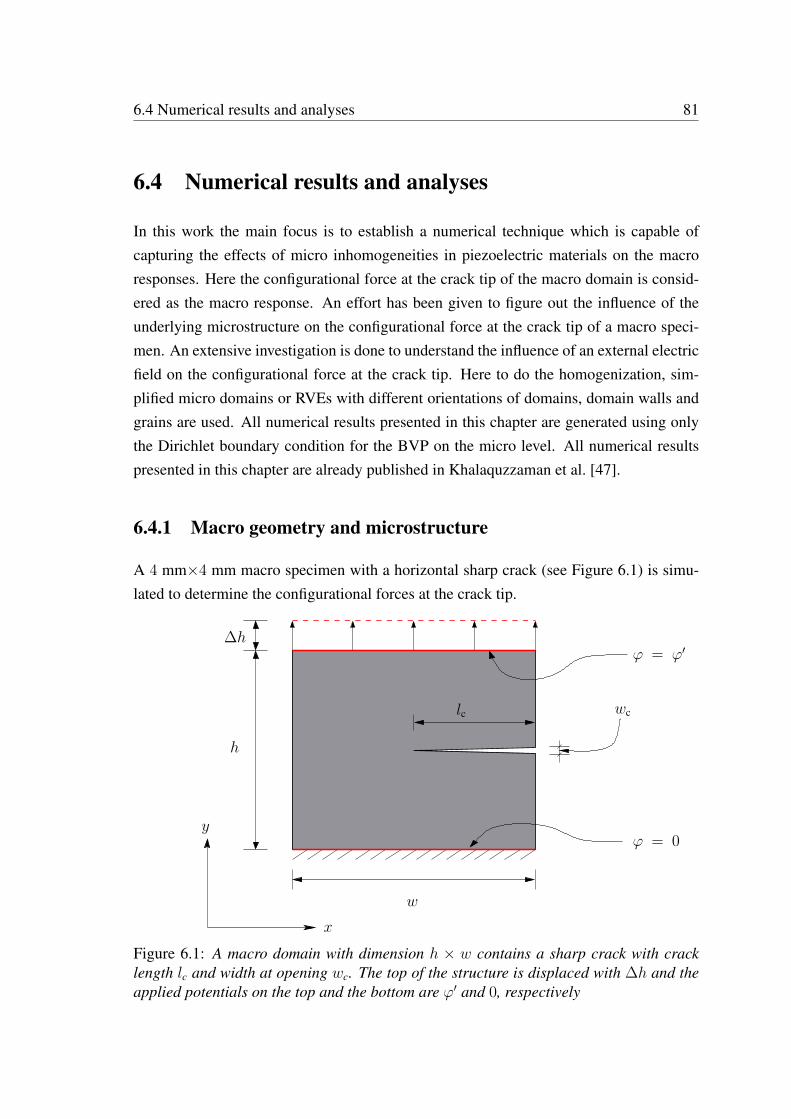
6.4 Numerical results and analyses 81
6.4 Numerical results and analyses
In this work the main focus is to establish a numerical technique which is capable ofcapturing the effects of micro inhomogeneities in piezoelectric materials on the macroresponses. Here the configurational force at the crack tip of the macro domain is consid-ered as the macro response. An effort has been given to figure out the influence of theunderlying microstructure on the configurational force at the crack tip of a macro speci-men. An extensive investigation is done to understand the influence of an external electricfield on the configurational force at the crack tip. Here to do the homogenization, sim-plified micro domains or RVEs with different orientations of domains, domain walls andgrains are used. All numerical results presented in this chapter are generated using onlythe Dirichlet boundary condition for the BVP on the micro level. All numerical resultspresented in this chapter are already published in Khalaquzzaman et al. [47].
6.4.1 Macro geometry and microstructure
A 4 mm×4 mm macro specimen with a horizontal sharp crack (see Figure 6.1) is simu-lated to determine the configurational forces at the crack tip.
w
h
∆h
lc wc
y
x
ϕ = ϕ′
ϕ = 0
Figure 6.1: A macro domain with dimension h × w contains a sharp crack with cracklength lc and width at opening wc. The top of the structure is displaced with ∆h and theapplied potentials on the top and the bottom are ϕ′ and 0, respectively
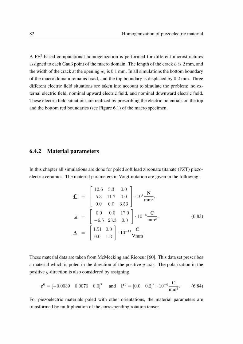
82 Homogenization of piezoelectric material
A FE2-based computational homogenization is performed for different microstructuresassigned to each Gauß point of the macro domain. The length of the crack lc is 2 mm, andthe width of the crack at the openingwc is 0.1 mm. In all simulations the bottom boundaryof the macro domain remains fixed, and the top boundary is displaced by 0.2 mm. Threedifferent electric field situations are taken into account to simulate the problem: no ex-ternal electric field, nominal upward electric field, and nominal downward electric field.These electric field situations are realized by prescribing the electric potentials on the topand the bottom red boundaries (see Figure 6.1) of the macro specimen.
6.4.2 Material parameters
In this chapter all simulations are done for poled soft lead zirconate titanate (PZT) piezo-electric ceramics. The material parameters in Voigt-notation are given in the following:
C =
12.6 5.3 0.0
5.3 11.7 0.0
0.0 0.0 3.53
· 104 N
mm2,
b =
[0.0 0.0 17.0
−6.5 23.3 0.0
]· 10−6 C
mm2, (6.83)
A =
[1.51 0.0
0.0 1.3
]· 10−11 C
Vmm.
These material data are taken from McMeeking and Ricoeur [60]. This data set prescribesa material which is poled in the direction of the positive y-axis. The polarization in thepositive y-direction is also considered by assigning
ε0 = [−0.0039 0.0076 0.0]T and P0 = [0.0 0.2]T · 10−6 Cmm2
. (6.84)
For piezoelectric materials poled with other orientations, the material parameters aretransformed by multiplication of the corresponding rotation tensor.
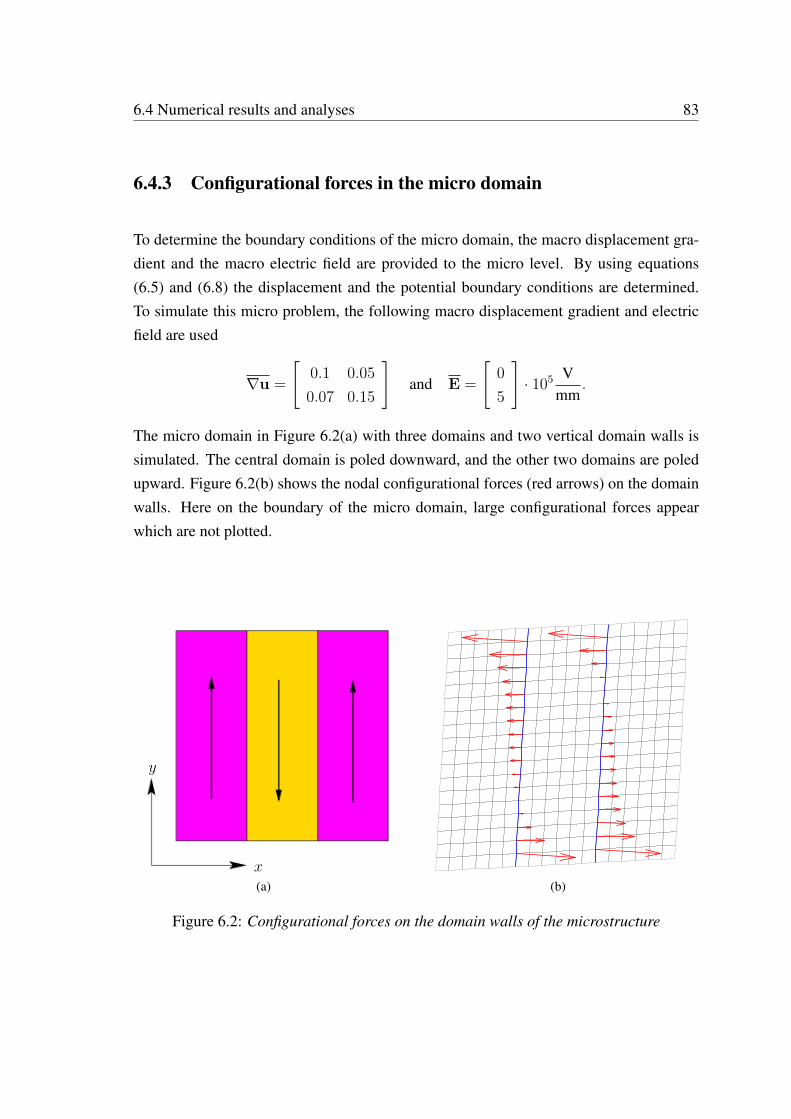
6.4 Numerical results and analyses 83
6.4.3 Configurational forces in the micro domain
To determine the boundary conditions of the micro domain, the macro displacement gra-dient and the macro electric field are provided to the micro level. By using equations(6.5) and (6.8) the displacement and the potential boundary conditions are determined.To simulate this micro problem, the following macro displacement gradient and electricfield are used
∇u =
[0.1 0.05
0.07 0.15
]and E =
[0
5
]· 105 V
mm.
The micro domain in Figure 6.2(a) with three domains and two vertical domain walls issimulated. The central domain is poled downward, and the other two domains are poledupward. Figure 6.2(b) shows the nodal configurational forces (red arrows) on the domainwalls. Here on the boundary of the micro domain, large configurational forces appearwhich are not plotted.
y
x(a) (b)
Figure 6.2: Configurational forces on the domain walls of the microstructure
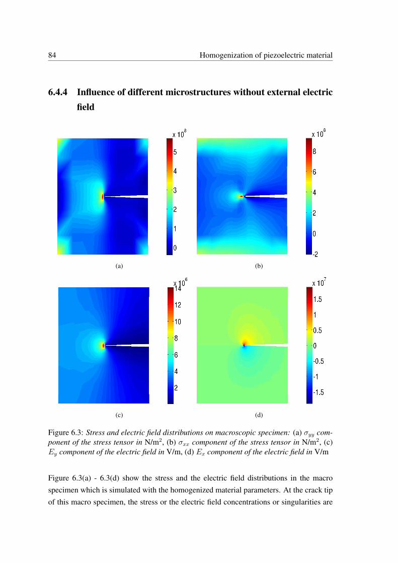
84 Homogenization of piezoelectric material
6.4.4 Influence of different microstructures without external electricfield
(a) (b)
(c) (d)
Figure 6.3: Stress and electric field distributions on macroscopic specimen: (a) σyy com-ponent of the stress tensor in N/m2, (b) σxx component of the stress tensor in N/m2, (c)Ey component of the electric field in V/m, (d) Ex component of the electric field in V/m
Figure 6.3(a) - 6.3(d) show the stress and the electric field distributions in the macrospecimen which is simulated with the homogenized material parameters. At the crack tipof this macro specimen, the stress or the electric field concentrations or singularities are
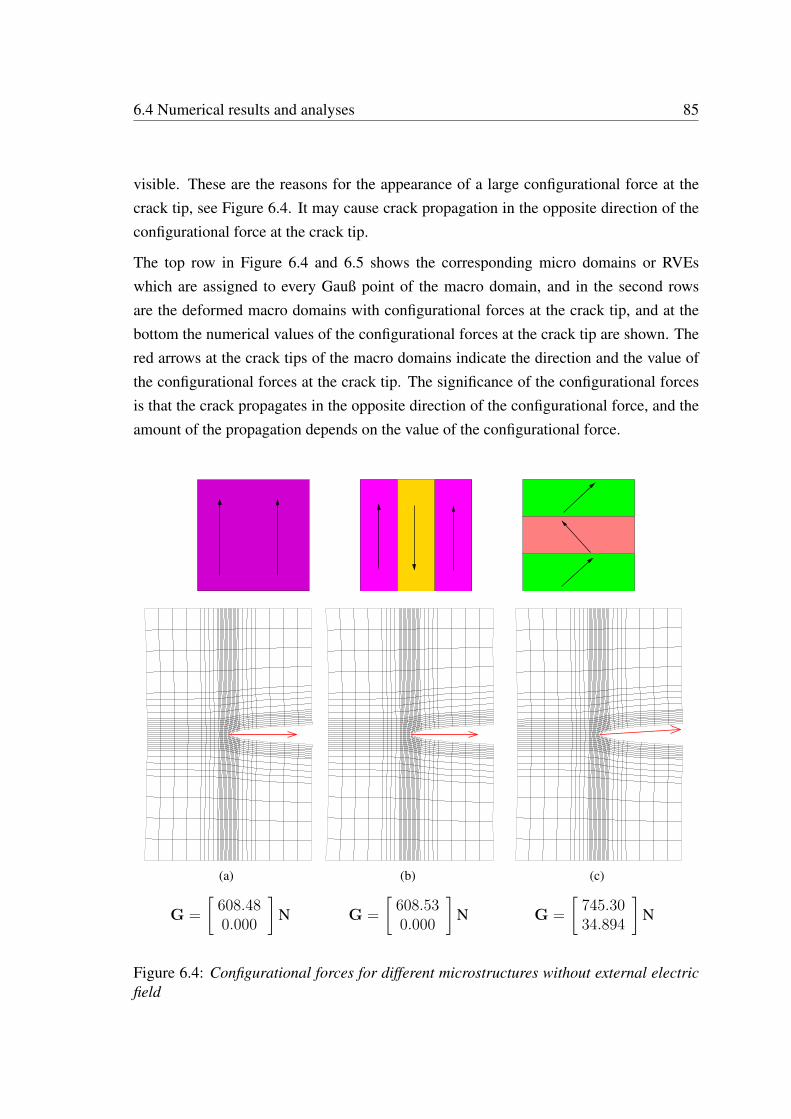
6.4 Numerical results and analyses 85
visible. These are the reasons for the appearance of a large configurational force at thecrack tip, see Figure 6.4. It may cause crack propagation in the opposite direction of theconfigurational force at the crack tip.
The top row in Figure 6.4 and 6.5 shows the corresponding micro domains or RVEswhich are assigned to every Gauß point of the macro domain, and in the second rowsare the deformed macro domains with configurational forces at the crack tip, and at thebottom the numerical values of the configurational forces at the crack tip are shown. Thered arrows at the crack tips of the macro domains indicate the direction and the value ofthe configurational forces at the crack tip. The significance of the configurational forcesis that the crack propagates in the opposite direction of the configurational force, and theamount of the propagation depends on the value of the configurational force.
(a) (b) (c)
G =
[608.480.000
]N G =
[608.530.000
]N G =
[745.3034.894
]N
Figure 6.4: Configurational forces for different microstructures without external electricfield
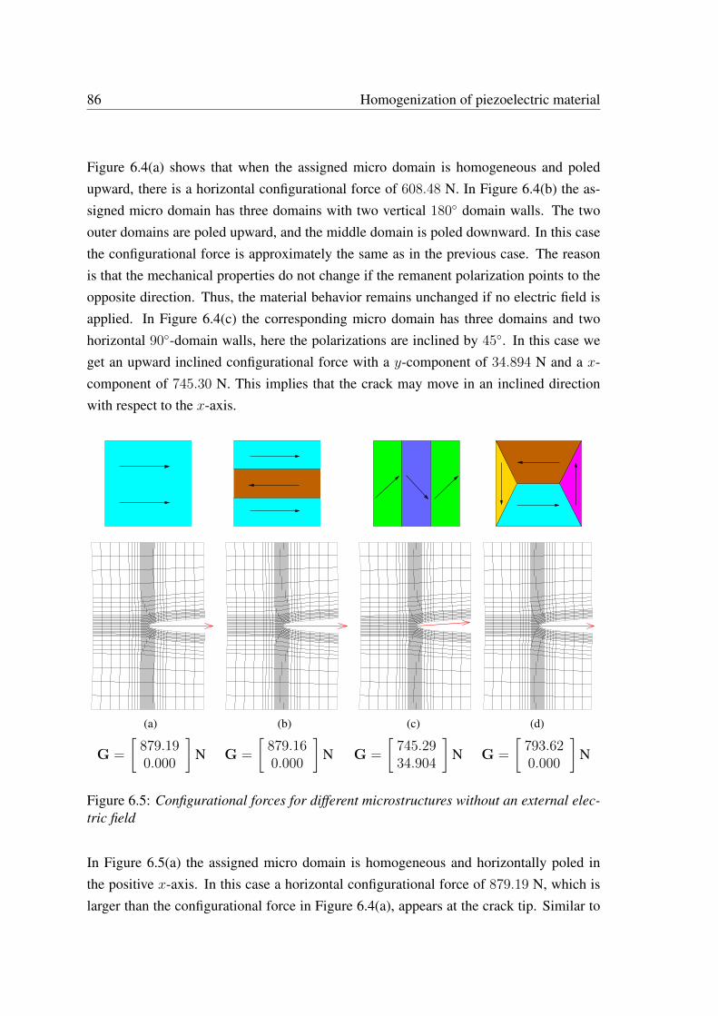
86 Homogenization of piezoelectric material
Figure 6.4(a) shows that when the assigned micro domain is homogeneous and poledupward, there is a horizontal configurational force of 608.48 N. In Figure 6.4(b) the as-signed micro domain has three domains with two vertical 180 domain walls. The twoouter domains are poled upward, and the middle domain is poled downward. In this casethe configurational force is approximately the same as in the previous case. The reasonis that the mechanical properties do not change if the remanent polarization points to theopposite direction. Thus, the material behavior remains unchanged if no electric field isapplied. In Figure 6.4(c) the corresponding micro domain has three domains and twohorizontal 90-domain walls, here the polarizations are inclined by 45. In this case weget an upward inclined configurational force with a y-component of 34.894 N and a x-component of 745.30 N. This implies that the crack may move in an inclined directionwith respect to the x-axis.
(a) (b) (c) (d)
G =
[879.190.000
]N G =
[879.160.000
]N G =
[745.2934.904
]N G =
[793.620.000
]N
Figure 6.5: Configurational forces for different microstructures without an external elec-tric field
In Figure 6.5(a) the assigned micro domain is homogeneous and horizontally poled inthe positive x-axis. In this case a horizontal configurational force of 879.19 N, which islarger than the configurational force in Figure 6.4(a), appears at the crack tip. Similar to
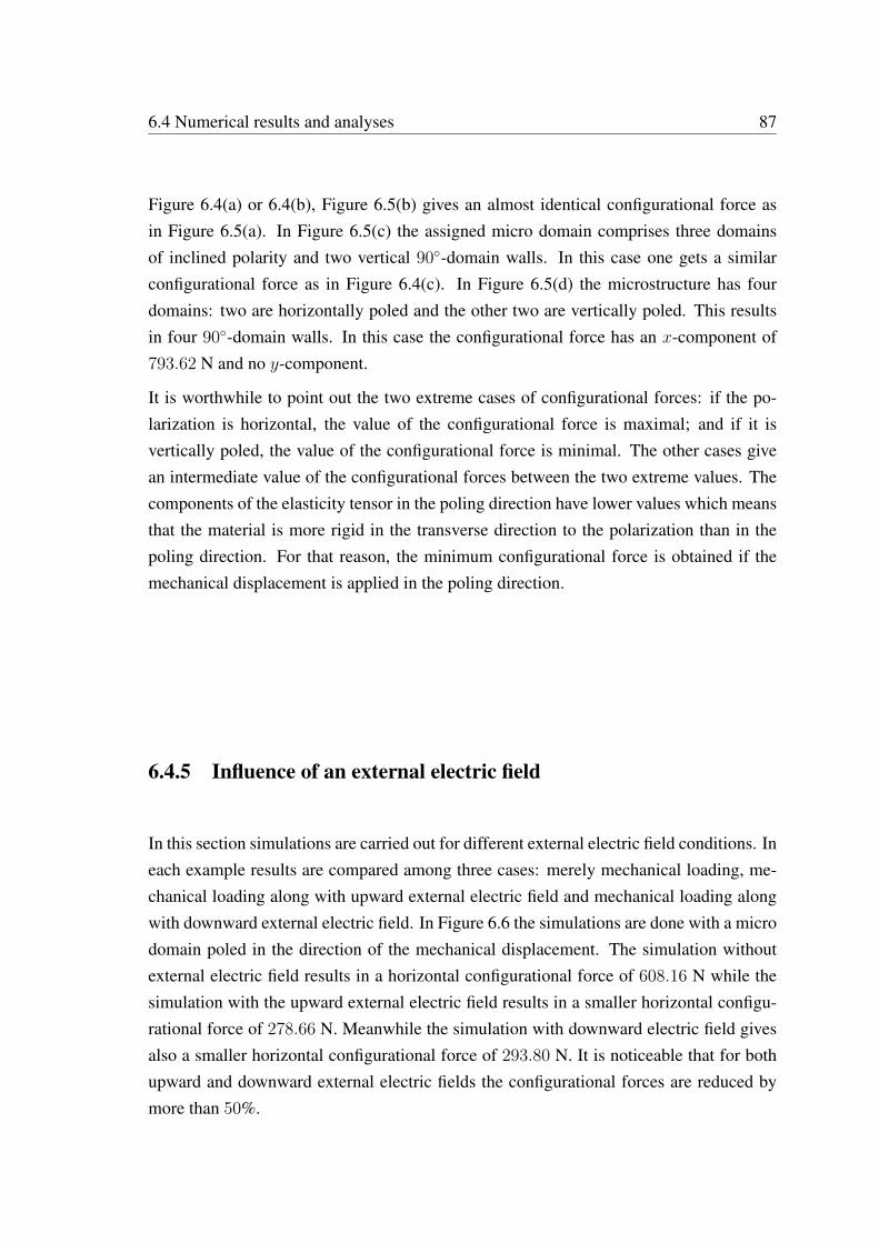
6.4 Numerical results and analyses 87
Figure 6.4(a) or 6.4(b), Figure 6.5(b) gives an almost identical configurational force asin Figure 6.5(a). In Figure 6.5(c) the assigned micro domain comprises three domainsof inclined polarity and two vertical 90-domain walls. In this case one gets a similarconfigurational force as in Figure 6.4(c). In Figure 6.5(d) the microstructure has fourdomains: two are horizontally poled and the other two are vertically poled. This resultsin four 90-domain walls. In this case the configurational force has an x-component of793.62 N and no y-component.
It is worthwhile to point out the two extreme cases of configurational forces: if the po-larization is horizontal, the value of the configurational force is maximal; and if it isvertically poled, the value of the configurational force is minimal. The other cases givean intermediate value of the configurational forces between the two extreme values. Thecomponents of the elasticity tensor in the poling direction have lower values which meansthat the material is more rigid in the transverse direction to the polarization than in thepoling direction. For that reason, the minimum configurational force is obtained if themechanical displacement is applied in the poling direction.
6.4.5 Influence of an external electric field
In this section simulations are carried out for different external electric field conditions. Ineach example results are compared among three cases: merely mechanical loading, me-chanical loading along with upward external electric field and mechanical loading alongwith downward external electric field. In Figure 6.6 the simulations are done with a microdomain poled in the direction of the mechanical displacement. The simulation withoutexternal electric field results in a horizontal configurational force of 608.16 N while thesimulation with the upward external electric field results in a smaller horizontal configu-rational force of 278.66 N. Meanwhile the simulation with downward electric field givesalso a smaller horizontal configurational force of 293.80 N. It is noticeable that for bothupward and downward external electric fields the configurational forces are reduced bymore than 50%.
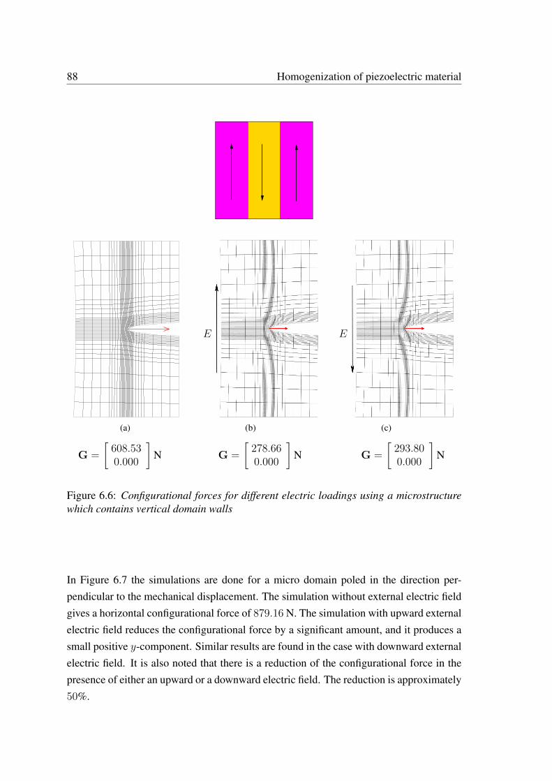
88 Homogenization of piezoelectric material
(a)
E
(b)
E
(c)
G =
[608.530.000
]N G =
[278.660.000
]N G =
[293.800.000
]N
Figure 6.6: Configurational forces for different electric loadings using a microstructurewhich contains vertical domain walls
In Figure 6.7 the simulations are done for a micro domain poled in the direction per-pendicular to the mechanical displacement. The simulation without external electric fieldgives a horizontal configurational force of 879.16 N. The simulation with upward externalelectric field reduces the configurational force by a significant amount, and it produces asmall positive y-component. Similar results are found in the case with downward externalelectric field. It is also noted that there is a reduction of the configurational force in thepresence of either an upward or a downward electric field. The reduction is approximately50%.
6.4 Numerical results and analyses 89
(a)
E
(b)
E
(c)
G =
[879.160.000
]N G =
[488.224.183
]N G =
[488.22−4.183
]N
Figure 6.7: Configurational forces for different electric loading using a microstructurewhich contains horizontal domain walls
All previous simulations were done for simple micro domains or RVEs. These microdomains or RVEs may not represent the real situation of the micro inhomogeneities ofpiezoelectric materials. The microstructures in real problems feature complex inhomo-geneities, for example domains, domain walls, micro cracks, grains, grain boundaries,etc. In attempt to obtain a better approximation of the real situation regarding the microinhomogeneities, the micro domain in Figure 6.8 is used. In this micro domain there arefive grains enclosed by the boundaries (red). Each grain features domains and domainwalls. When the simulation is done only for mechanical displacement, a configurationalforce with an x-component of 741.97 N and a y-component of −33.168 N is obtained.These values imply that the crack may propagate in an inclined direction to the x-axis.
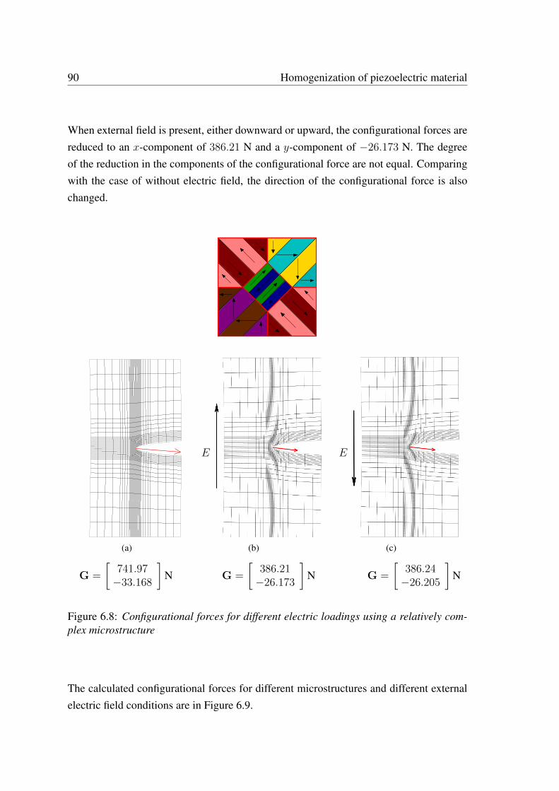
90 Homogenization of piezoelectric material
When external field is present, either downward or upward, the configurational forces arereduced to an x-component of 386.21 N and a y-component of −26.173 N. The degreeof the reduction in the components of the configurational force are not equal. Comparingwith the case of without electric field, the direction of the configurational force is alsochanged.
(a)
E
(b)
E
(c)
G =
[741.97−33.168
]N G =
[386.21−26.173
]N G =
[386.24−26.205
]N
Figure 6.8: Configurational forces for different electric loadings using a relatively com-plex microstructure
The calculated configurational forces for different microstructures and different externalelectric field conditions are in Figure 6.9.
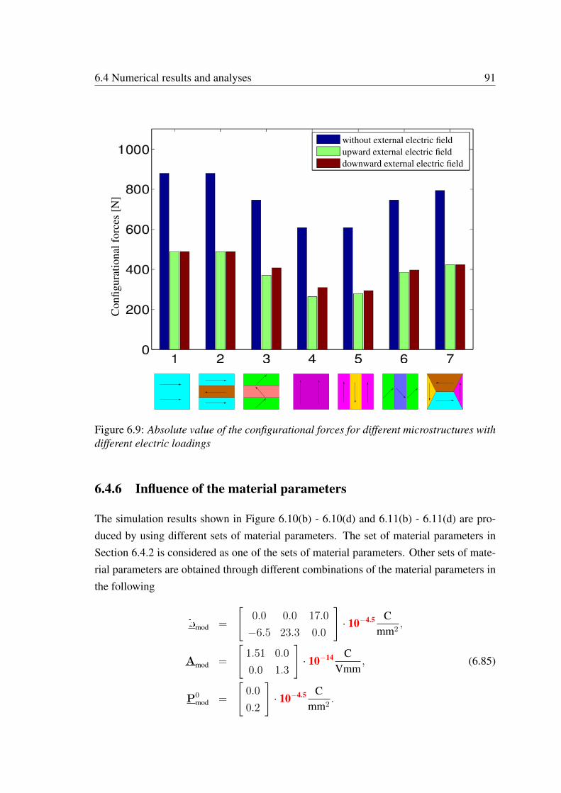
6.4 Numerical results and analyses 91
Con
figur
atio
nalf
orce
s[N
]
without external electric fieldupward external electric fielddownward external electric field
Figure 6.9: Absolute value of the configurational forces for different microstructures withdifferent electric loadings
6.4.6 Influence of the material parameters
The simulation results shown in Figure 6.10(b) - 6.10(d) and 6.11(b) - 6.11(d) are pro-duced by using different sets of material parameters. The set of material parameters inSection 6.4.2 is considered as one of the sets of material parameters. Other sets of mate-rial parameters are obtained through different combinations of the material parameters inthe following
bmod =
[0.0 0.0 17.0
−6.5 23.3 0.0
]· 10−4.5 C
mm2,
Amod =
[1.51 0.0
0.0 1.3
]· 10−14 C
Vmm, (6.85)
P0mod =
[0.0
0.2
]· 10−4.5 C
mm2.
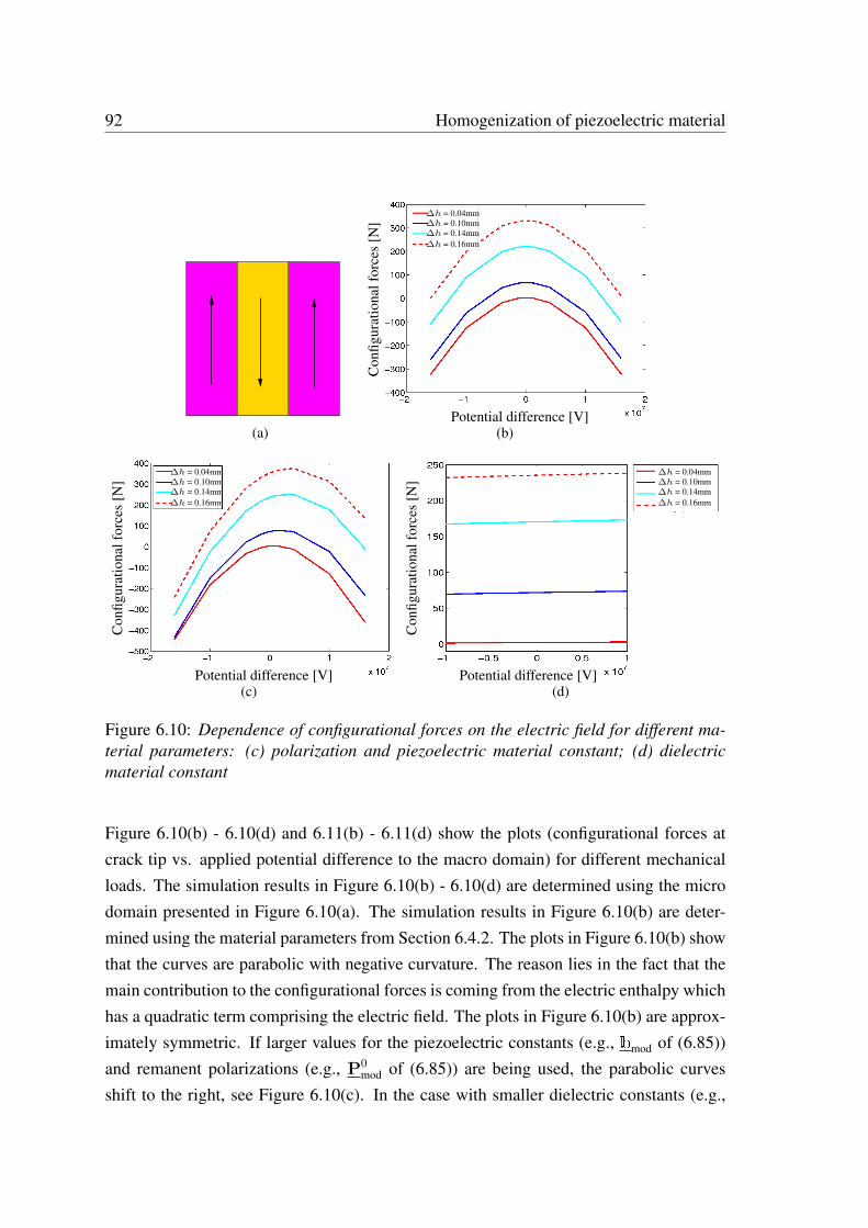
92 Homogenization of piezoelectric material
(a)
Con
figur
atio
nalf
orce
s[N
]
Potential difference [V]
∆h = 0.04mm∆h = 0.10mm∆h = 0.14mm∆h = 0.16mm
(b)
Con
figur
atio
nalf
orce
s[N
]
Potential difference [V]
∆h = 0.04mm∆h = 0.10mm∆h = 0.14mm∆h = 0.16mm
(c)
Con
figur
atio
nalf
orce
s[N
]
Potential difference [V]
∆h = 0.04mm∆h = 0.10mm∆h = 0.14mm∆h = 0.16mm
(d)
Figure 6.10: Dependence of configurational forces on the electric field for different ma-terial parameters: (c) polarization and piezoelectric material constant; (d) dielectricmaterial constant
Figure 6.10(b) - 6.10(d) and 6.11(b) - 6.11(d) show the plots (configurational forces atcrack tip vs. applied potential difference to the macro domain) for different mechanicalloads. The simulation results in Figure 6.10(b) - 6.10(d) are determined using the microdomain presented in Figure 6.10(a). The simulation results in Figure 6.10(b) are deter-mined using the material parameters from Section 6.4.2. The plots in Figure 6.10(b) showthat the curves are parabolic with negative curvature. The reason lies in the fact that themain contribution to the configurational forces is coming from the electric enthalpy whichhas a quadratic term comprising the electric field. The plots in Figure 6.10(b) are approx-imately symmetric. If larger values for the piezoelectric constants (e.g., bmod of (6.85))and remanent polarizations (e.g., P0
mod of (6.85)) are being used, the parabolic curvesshift to the right, see Figure 6.10(c). In the case with smaller dielectric constants (e.g.,
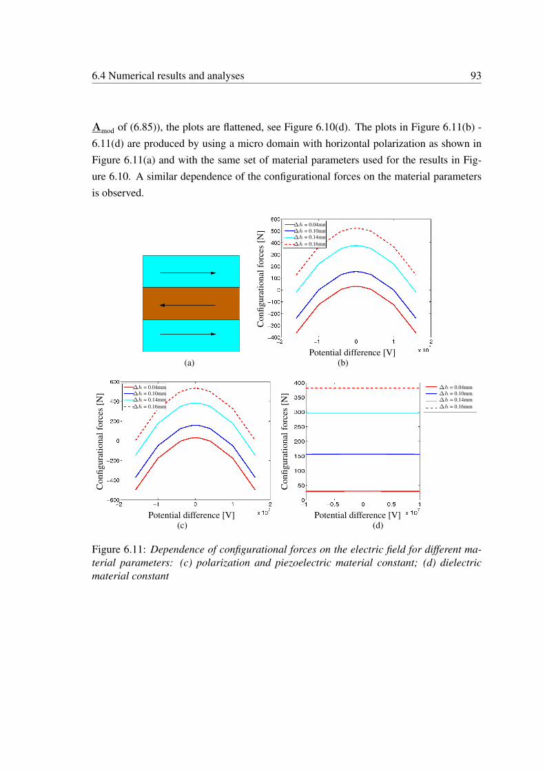
6.4 Numerical results and analyses 93
Amod of (6.85)), the plots are flattened, see Figure 6.10(d). The plots in Figure 6.11(b) -6.11(d) are produced by using a micro domain with horizontal polarization as shown inFigure 6.11(a) and with the same set of material parameters used for the results in Fig-ure 6.10. A similar dependence of the configurational forces on the material parametersis observed.
(a)
Con
figur
atio
nalf
orce
s[N
]
Potential difference [V]
∆h = 0.04mm∆h = 0.10mm∆h = 0.14mm∆h = 0.16mm
(b)
Con
figur
atio
nalf
orce
s[N
]
Potential difference [V]
∆h = 0.04mm∆h = 0.10mm∆h = 0.14mm∆h = 0.16mm
(c)
Con
figur
atio
nalf
orce
s[N
]
Potential difference [V]
∆h = 0.04mm∆h = 0.10mm∆h = 0.14mm∆h = 0.16mm
(d)
Figure 6.11: Dependence of configurational forces on the electric field for different ma-terial parameters: (c) polarization and piezoelectric material constant; (d) dielectricmaterial constant

94 Homogenization of piezoelectric material
Chapter 7
Homogenization of piezoelectricmaterials using evolvingmicrostructures
In the previous chapter, the investigation of the configurational forces at the macro cracktip was carried out using a fixed or non-evolving microstructure as the representative vol-ume element (RVE). In other words, the movement of the domain wall was neglected.But in real situations, one has no direct control over the movement of the domain walls.The movement of the interface can be induced by an external electric and/or mechanicalloading. If an electric field larger than the critical electric field is applied to a piezoelectricspecimen, the domain walls can move. Thus, homogenization using evolving microstruc-tures is required to obtain physically more accurate simulation results. As a consequenceof the evolution of the microstructure, it is necessary to update the micro domain at everystep of the homogenization during the the application of a varying electric field.
7.1 Domain wall driving force and interface kinetics
As stated previously, domain walls in ferroelectric materials can be modeled in two differ-ent ways: one is the sharp interface approach, and the other one is the phase field modelapproach. Here the sharp interface approach is used. The assumption for the sharp in-
96 Homogenization using evolving microstructures
terface model is that each ferroelectric domain is considered as a homogeneous domainand is separated by a domain wall with zero thickness. For this reason the geometry ofthe domain wall S can be seen as an internal variable of the electric enthalpy. For a RVEwith a single interface, the dependence of the electric enthalpy on this position can beexpressed by
H(ε,E,X;S) =1
2(ε− ε0
±):[C±(ε− ε0
±)]− (ε− ε0
±): (bT±E)
−1
2E·(A±E)−P0
± ·E, (7.1)
where the material parameter (·)+ is considered if X ∈ B+ and (·)− is considered ifX ∈ B− (see Figure 4.1).
Recalling the Eshelby stress tensor for piezoelectric materials
Σ = H 1− (∇u)Tσ −∇ϕ⊗D, (7.2)
the configurational force balance (4.25) can be reduced in this case to the jump relation
JΣKnS + GS = 0, (7.3)
where GS is the surface configurational force acting on the domain wall, i.e. a force perunit area, and nS is the normal vector to the domain wall pointing towards the domainB+, see Figure 4.1. If the domain wall moves with velocity wS , the energy dissipationdue to this movement is given by
D = −∫
SGS ·wSdΓ =
∫
SτnwndΓ > 0. (7.4)
Hereby the fact is considered that only the normal component of the configurational forceon the interface has a contribution to the dissipation. In the above equation the followingquantities are used,
τn = −GS ·nS = nS ·JΣKnS and wn = wS ·nS . (7.5)
7.1 Domain wall driving force and interface kinetics 97
Recalling the resulting configurational force at node K, which was obtained by assem-bling all ne elements adjacent to node K, we have
GK =ne⋃
e=1
GKe . (7.6)
The normal component of the configurational force Gn acting on the interface S is formu-lated by
Gn =∑
K
GKS ·nS , (7.7)
where the summation includes all nodes located on the interface S. Furthermore, scalarmultiplication of the balance of configurational forces on S in (7.3) with −nS/AS andintegration over S leads to
− 1
AS
∫
SGS ·nSdΓ =
1
AS
∫
SτndΓ = Tn. (7.8)
With the help of the finite element approximation (4.36), the average domain wall drivingforce on S is determined from
Tn = − 1
AS
∫
SGS ·nSdΓ = − 1
AS
∑
K
GKS ·nS = − 1
ASGn. (7.9)
The formulations shown above do not state a specific kinetic law for the interface normalvelocity wn. To establish such a relationship, experimental investigations by Flippen [21]are taken into consideration. In these experiments the dynamics of the 180 domain wallbetween two domains in Gadolinium Molybdate (GMO) single crystal was investigated,in that a domain wall was relocated through the material by applying an external homo-geneous electric field E parallel to the interface or the domain wall. The measurementsshow a linear relationship between the interface velocity wn and the electric field E. Thekinetic law can be formulated in terms of the applied electric field by
wn = µ(E − E0). (7.10)
The parameter µ denotes the mobility of the domain wall or the interface, and E0 isthe threshold or critical electric field for domain wall movement. It is noted that thissimplified relation is only applicable for the homogeneous electric field. In the case ofinhomogeneous fields, which are present in general, and with the consideration of the
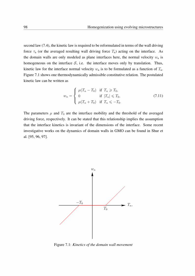
98 Homogenization using evolving microstructures
second law (7.4), the kinetic law is required to be reformulated in terms of the wall drivingforce τn (or the averaged resulting wall driving force Tn) acting on the interface. Asthe domain walls are only modeled as plane interfaces here, the normal velocity wn ishomogeneous on the interface S, i.e. the interface moves only by translation. Thus,kinetic law for the interface normal velocity wn is to be formulated as a function of Tn.Figure 7.1 shows one thermodynamically admissible constitutive relation. The postulatedkinetic law can be written as
wn =
µ(Tn − T0) if Tn > T0,
0 if |Tn| 6 T0,
µ(Tn + T0) if Tn 6 −T0.
(7.11)
The parameters µ and T0 are the interface mobility and the threshold of the averageddriving force, respectively. It can be stated that this relationship implies the assumptionthat the interface kinetics is invariant of the dimensions of the interface. Some recentinvestigative works on the dynamics of domain walls in GMO can be found in Shur etal. [95, 96, 97].
wn
Tn,T0
−T0
Figure 7.1: Kinetics of the domain wall movement
7.1 Domain wall driving force and interface kinetics 99
The wall driving force on a 180-domain wall in the presence of an external electric fieldE parallel to the interface can be determined from (7.5). As derived in Appendix A.4.1,this wall driving force is approximated by
τn ≈ JP0 ·EK = 2P 0E, (7.12)
where P 0 =| P0 |, see Loge and Suo [56]. The value of T0 is determined from (7.8) and(7.12) for E = E0
T0 =1
AS
∫
Sτn(E0)dΓ = τn(E0) = 2P 0E0. (7.13)
For E = 2E0 and evidently Tn = 2T0, the combination of (7.10) and (7.11) leads to
wn = µ(Tn − T0) = µT0 = 2µP 0E0 = µE0, (7.14)
which infersµ =
µ
2P 0. (7.15)
The value for µ and E0 can be found in Flippen [21].
Similarly, for a 90-domain wall,
τn ≈ JP0 ·EK = 2P 02E, (7.16)
where P 02 is the vertical component of P0. The threshold wall driving force T0 = 2P 0
2E0
and wall mobility parameter µ = µ/2P 02 .
7.1.1 Time integration
The Euler forward (or an explicit) time integration formula is applied to obtain a dis-cretized form of the kinetic law (7.11) in time. Hence the discretized position (only w.r.t.time) of the domain wall can be formulated as
Xn+1S = Xn
S + wnn4t, (7.17)
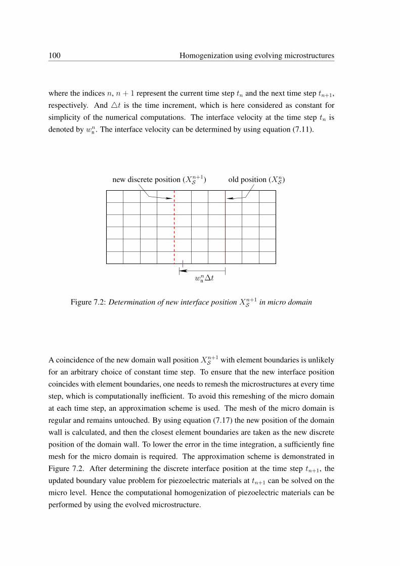
100 Homogenization using evolving microstructures
where the indices n, n + 1 represent the current time step tn and the next time step tn+1,respectively. And 4t is the time increment, which is here considered as constant forsimplicity of the numerical computations. The interface velocity at the time step tn isdenoted by wnn . The interface velocity can be determined by using equation (7.11).
old position (XnS )new discrete position (Xn+1
S )
wnn ∆t
Figure 7.2: Determination of new interface position Xn+1S in micro domain
A coincidence of the new domain wall position Xn+1S with element boundaries is unlikely
for an arbitrary choice of constant time step. To ensure that the new interface positioncoincides with element boundaries, one needs to remesh the microstructures at every timestep, which is computationally inefficient. To avoid this remeshing of the micro domainat each time step, an approximation scheme is used. The mesh of the micro domain isregular and remains untouched. By using equation (7.17) the new position of the domainwall is calculated, and then the closest element boundaries are taken as the new discreteposition of the domain wall. To lower the error in the time integration, a sufficiently finemesh for the micro domain is required. The approximation scheme is demonstrated inFigure 7.2. After determining the discrete interface position at the time step tn+1, theupdated boundary value problem for piezoelectric materials at tn+1 can be solved on themicro level. Hence the computational homogenization of piezoelectric materials can beperformed by using the evolved microstructure.
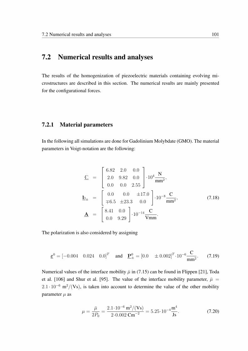
7.2 Numerical results and analyses 101
7.2 Numerical results and analyses
The results of the homogenization of piezoelectric materials containing evolving mi-crostructures are described in this section. The numerical results are mainly presentedfor the configurational forces.
7.2.1 Material parameters
In the following all simulations are done for Gadolinium Molybdate (GMO). The materialparameters in Voigt-notation are the following:
C =
6.82 2.0 0.0
2.0 9.82 0.0
0.0 0.0 2.55
·104 N
mm2,
b± =
[0.0 0.0 ±17.0
∓6.5 ±23.3 0.0
]·10−8 C
mm2, (7.18)
A =
[8.41 0.0
0.0 9.29
]·10−14 C
Vmm.
The polarization is also considered by assigning
ε0 = [−0.004 0.024 0.0]T and P0± = [0.0 ± 0.002]T ·10−6 C
mm2. (7.19)
Numerical values of the interface mobility µ in (7.15) can be found in Flippen [21], Todaet al. [106] and Shur et al. [95]. The value of the interface mobility parameter, µ =
2.1 · 10−6 m2/(Vs), is taken into account to determine the value of the other mobilityparameter µ as
µ =µ
2P0
=2.1·10−6 m2/(Vs)
2·0.002 Cm−2 = 5.25·10−4 m4
Js. (7.20)
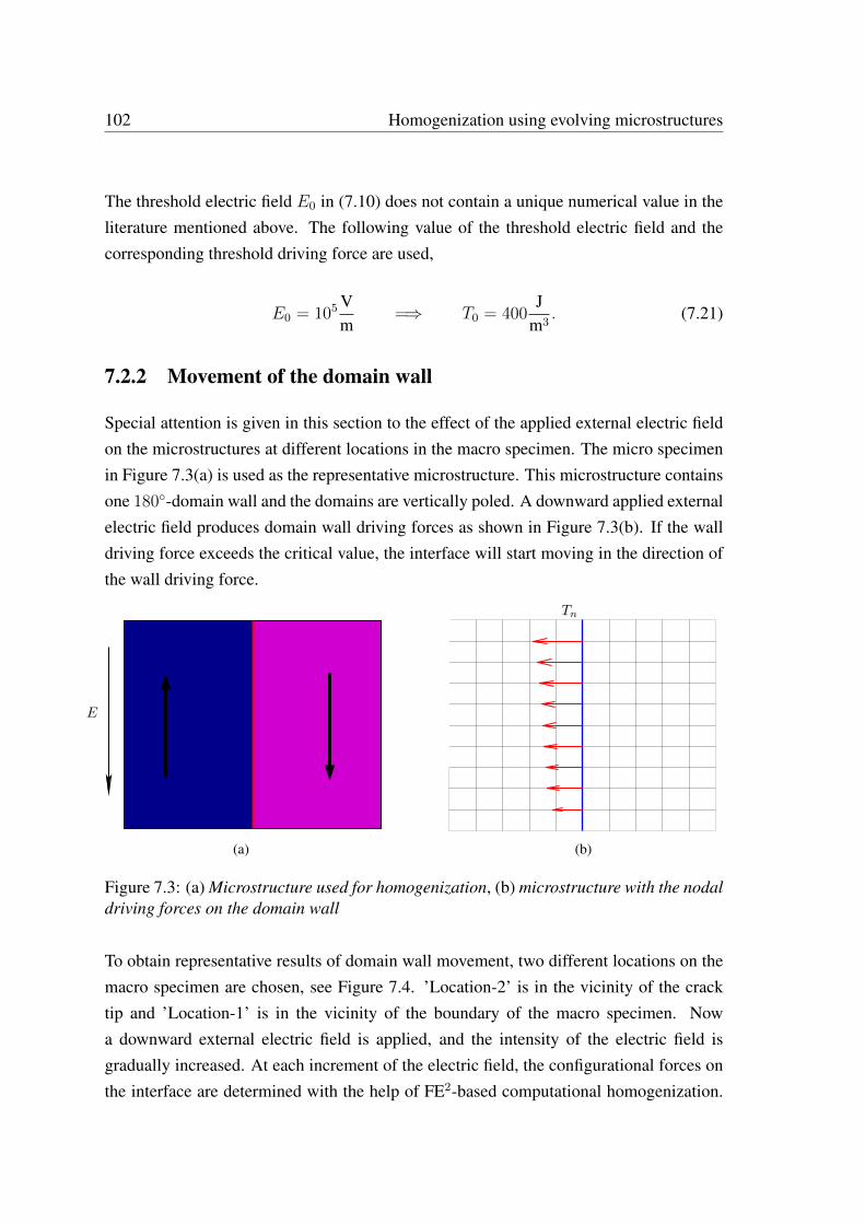
102 Homogenization using evolving microstructures
The threshold electric field E0 in (7.10) does not contain a unique numerical value in theliterature mentioned above. The following value of the threshold electric field and thecorresponding threshold driving force are used,
E0 = 105 Vm
=⇒ T0 = 400J
m3. (7.21)
7.2.2 Movement of the domain wall
Special attention is given in this section to the effect of the applied external electric fieldon the microstructures at different locations in the macro specimen. The micro specimenin Figure 7.3(a) is used as the representative microstructure. This microstructure containsone 180-domain wall and the domains are vertically poled. A downward applied externalelectric field produces domain wall driving forces as shown in Figure 7.3(b). If the walldriving force exceeds the critical value, the interface will start moving in the direction ofthe wall driving force.
(a) (b)
E
Tn
Figure 7.3: (a) Microstructure used for homogenization, (b) microstructure with the nodaldriving forces on the domain wall
To obtain representative results of domain wall movement, two different locations on themacro specimen are chosen, see Figure 7.4. ’Location-2’ is in the vicinity of the cracktip and ’Location-1’ is in the vicinity of the boundary of the macro specimen. Nowa downward external electric field is applied, and the intensity of the electric field isgradually increased. At each increment of the electric field, the configurational forces onthe interface are determined with the help of FE2-based computational homogenization.
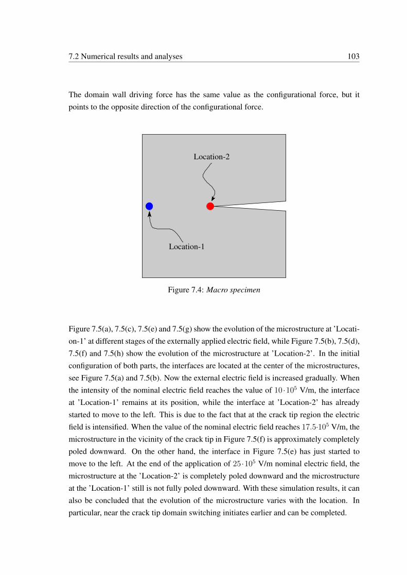
7.2 Numerical results and analyses 103
The domain wall driving force has the same value as the configurational force, but itpoints to the opposite direction of the configurational force.
Location-1
Location-2
Figure 7.4: Macro specimen
Figure 7.5(a), 7.5(c), 7.5(e) and 7.5(g) show the evolution of the microstructure at ’Locati-on-1’ at different stages of the externally applied electric field, while Figure 7.5(b), 7.5(d),7.5(f) and 7.5(h) show the evolution of the microstructure at ’Location-2’. In the initialconfiguration of both parts, the interfaces are located at the center of the microstructures,see Figure 7.5(a) and 7.5(b). Now the external electric field is increased gradually. Whenthe intensity of the nominal electric field reaches the value of 10 ·105 V/m, the interfaceat ’Location-1’ remains at its position, while the interface at ’Location-2’ has alreadystarted to move to the left. This is due to the fact that at the crack tip region the electricfield is intensified. When the value of the nominal electric field reaches 17.5·105 V/m, themicrostructure in the vicinity of the crack tip in Figure 7.5(f) is approximately completelypoled downward. On the other hand, the interface in Figure 7.5(e) has just started tomove to the left. At the end of the application of 25 ·105 V/m nominal electric field, themicrostructure at the ’Location-2’ is completely poled downward and the microstructureat the ’Location-1’ still is not fully poled downward. With these simulation results, it canalso be concluded that the evolution of the microstructure varies with the location. Inparticular, near the crack tip domain switching initiates earlier and can be completed.
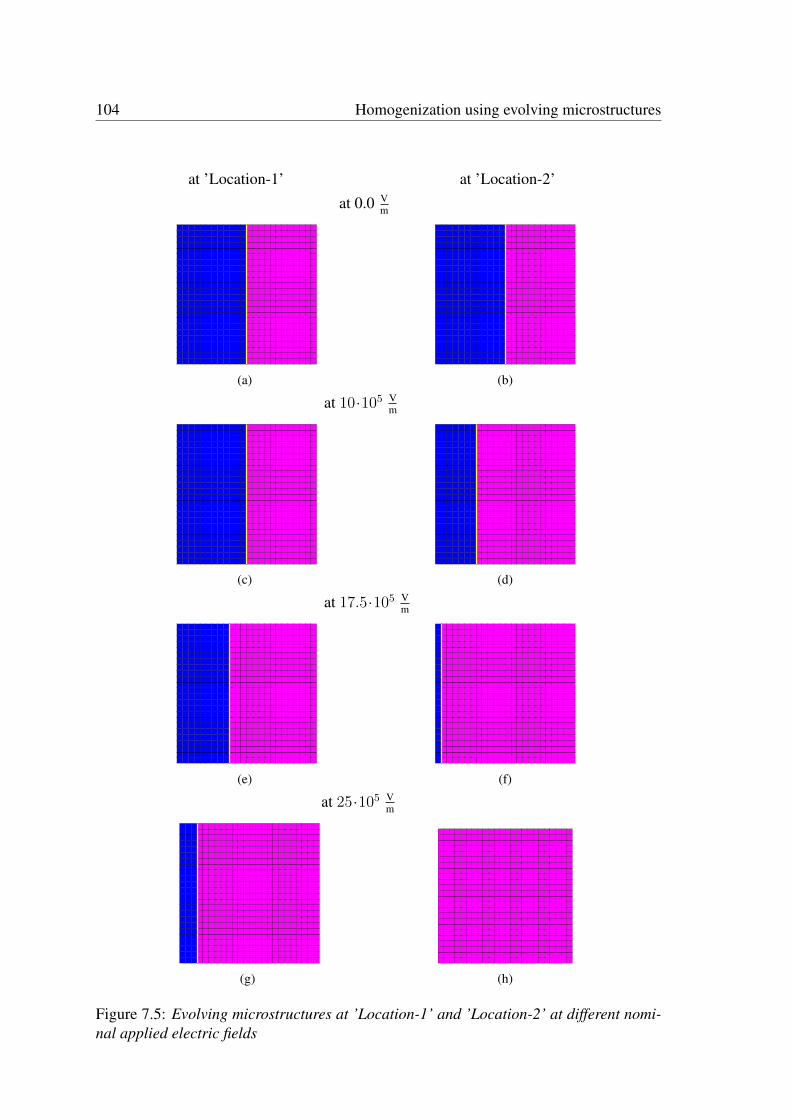
104 Homogenization using evolving microstructures
(a) (b)
at ’Location-1’ at ’Location-2’
at 0.0 Vm
(c) (d)
at 10·105 Vm
(e) (f)
at 17.5·105 Vm
(g) (h)
at 25·105 Vm
Figure 7.5: Evolving microstructures at ’Location-1’ and ’Location-2’ at different nomi-nal applied electric fields
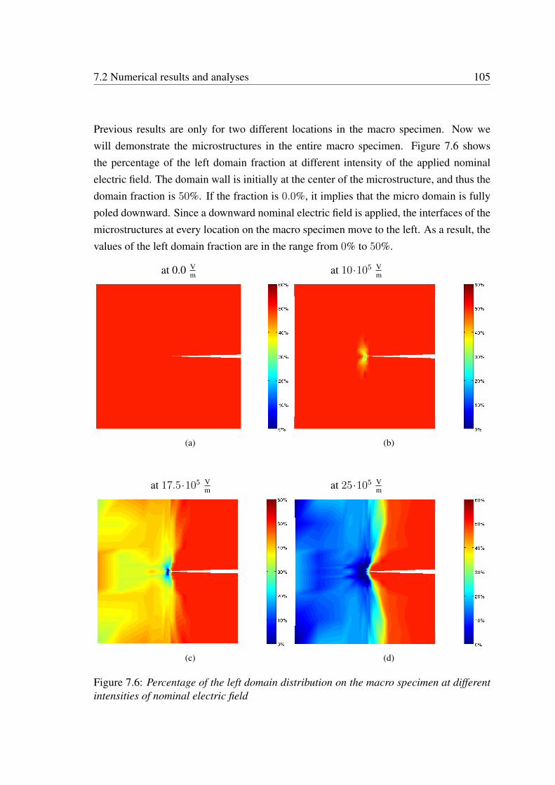
7.2 Numerical results and analyses 105
Previous results are only for two different locations in the macro specimen. Now wewill demonstrate the microstructures in the entire macro specimen. Figure 7.6 showsthe percentage of the left domain fraction at different intensity of the applied nominalelectric field. The domain wall is initially at the center of the microstructure, and thus thedomain fraction is 50%. If the fraction is 0.0%, it implies that the micro domain is fullypoled downward. Since a downward nominal electric field is applied, the interfaces of themicrostructures at every location on the macro specimen move to the left. As a result, thevalues of the left domain fraction are in the range from 0% to 50%.
(a) (b)
at 0.0 Vm at 10·105 V
m
(c) (d)
at 17.5·105 Vm at 25·105 V
m
Figure 7.6: Percentage of the left domain distribution on the macro specimen at differentintensities of nominal electric field
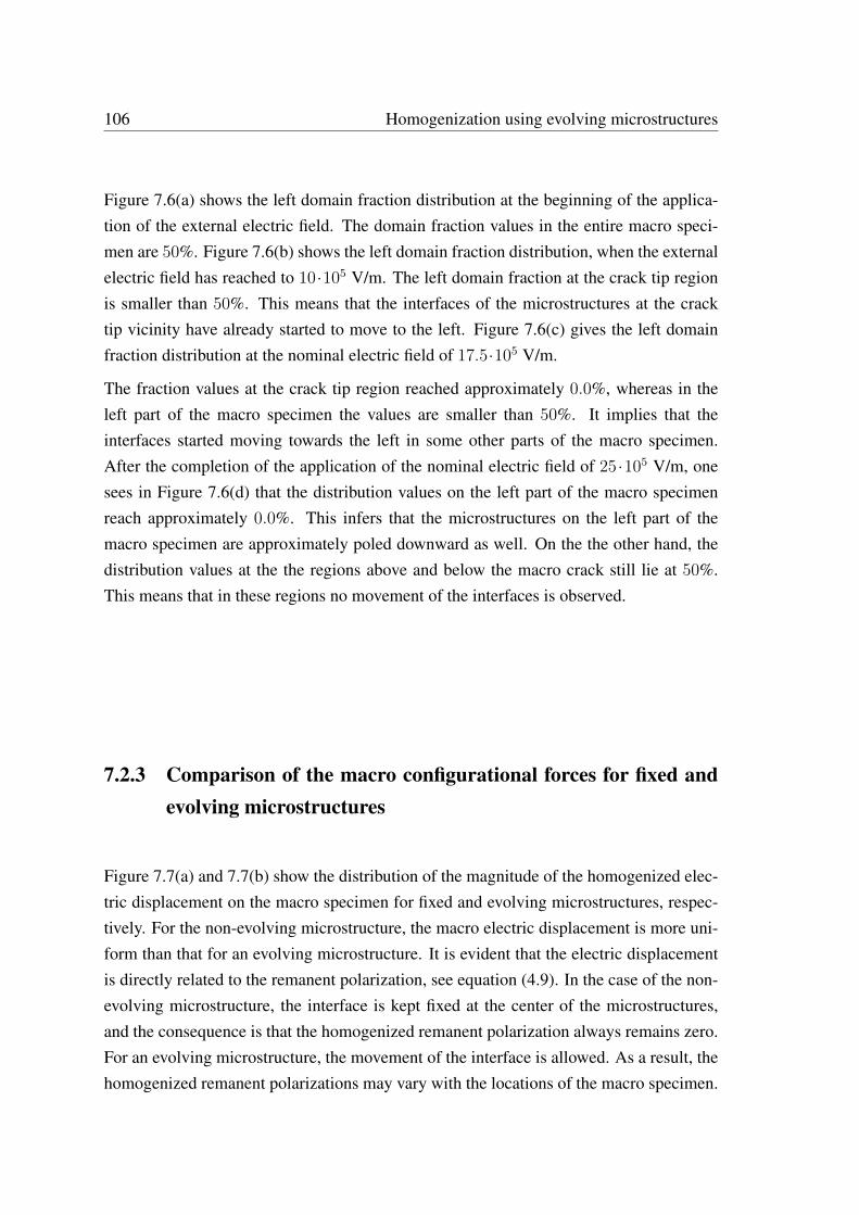
106 Homogenization using evolving microstructures
Figure 7.6(a) shows the left domain fraction distribution at the beginning of the applica-tion of the external electric field. The domain fraction values in the entire macro speci-men are 50%. Figure 7.6(b) shows the left domain fraction distribution, when the externalelectric field has reached to 10·105 V/m. The left domain fraction at the crack tip regionis smaller than 50%. This means that the interfaces of the microstructures at the cracktip vicinity have already started to move to the left. Figure 7.6(c) gives the left domainfraction distribution at the nominal electric field of 17.5·105 V/m.
The fraction values at the crack tip region reached approximately 0.0%, whereas in theleft part of the macro specimen the values are smaller than 50%. It implies that theinterfaces started moving towards the left in some other parts of the macro specimen.After the completion of the application of the nominal electric field of 25 ·105 V/m, onesees in Figure 7.6(d) that the distribution values on the left part of the macro specimenreach approximately 0.0%. This infers that the microstructures on the left part of themacro specimen are approximately poled downward as well. On the the other hand, thedistribution values at the the regions above and below the macro crack still lie at 50%.This means that in these regions no movement of the interfaces is observed.
7.2.3 Comparison of the macro configurational forces for fixed andevolving microstructures
Figure 7.7(a) and 7.7(b) show the distribution of the magnitude of the homogenized elec-tric displacement on the macro specimen for fixed and evolving microstructures, respec-tively. For the non-evolving microstructure, the macro electric displacement is more uni-form than that for an evolving microstructure. It is evident that the electric displacementis directly related to the remanent polarization, see equation (4.9). In the case of the non-evolving microstructure, the interface is kept fixed at the center of the microstructures,and the consequence is that the homogenized remanent polarization always remains zero.For an evolving microstructure, the movement of the interface is allowed. As a result, thehomogenized remanent polarizations may vary with the locations of the macro specimen.
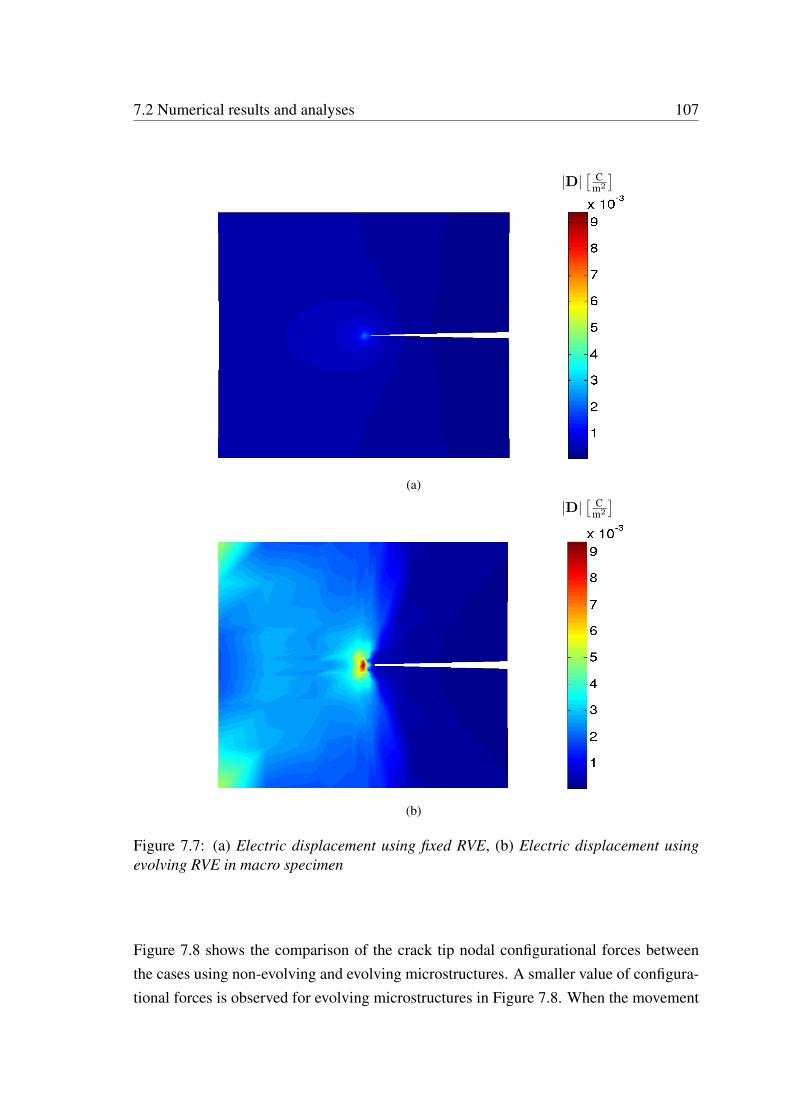
7.2 Numerical results and analyses 107
(a)
|D|[ C
m2
]
(b)
|D|[ C
m2
]
Figure 7.7: (a) Electric displacement using fixed RVE, (b) Electric displacement usingevolving RVE in macro specimen
Figure 7.8 shows the comparison of the crack tip nodal configurational forces betweenthe cases using non-evolving and evolving microstructures. A smaller value of configura-tional forces is observed for evolving microstructures in Figure 7.8. When the movement
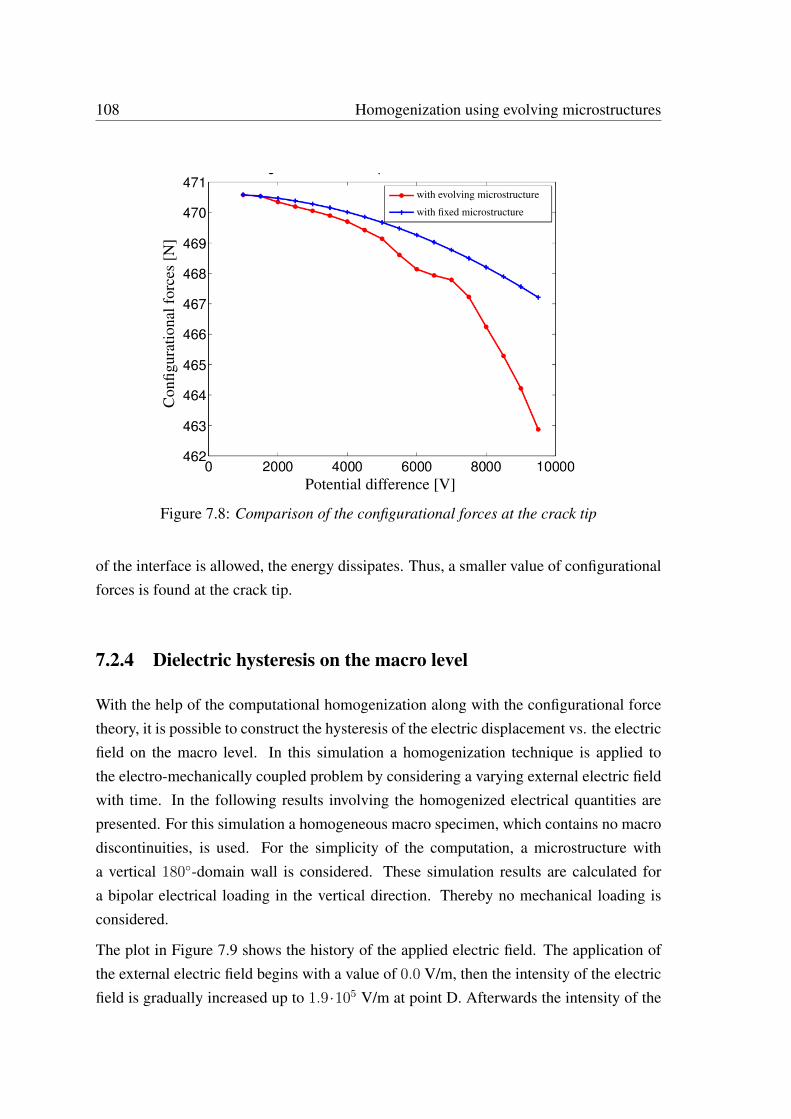
108 Homogenization using evolving microstructures
Con
figur
atio
nalf
orce
s[N
]
Potential difference [V]
with evolving microstructure
with fixed microstructure
Figure 7.8: Comparison of the configurational forces at the crack tip
of the interface is allowed, the energy dissipates. Thus, a smaller value of configurationalforces is found at the crack tip.
7.2.4 Dielectric hysteresis on the macro level
With the help of the computational homogenization along with the configurational forcetheory, it is possible to construct the hysteresis of the electric displacement vs. the electricfield on the macro level. In this simulation a homogenization technique is applied tothe electro-mechanically coupled problem by considering a varying external electric fieldwith time. In the following results involving the homogenized electrical quantities arepresented. For this simulation a homogeneous macro specimen, which contains no macrodiscontinuities, is used. For the simplicity of the computation, a microstructure witha vertical 180-domain wall is considered. These simulation results are calculated fora bipolar electrical loading in the vertical direction. Thereby no mechanical loading isconsidered.
The plot in Figure 7.9 shows the history of the applied electric field. The application ofthe external electric field begins with a value of 0.0 V/m, then the intensity of the electricfield is gradually increased up to 1.9·105 V/m at point D. Afterwards the intensity of the
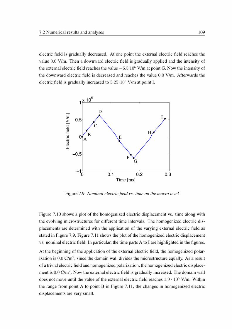
7.2 Numerical results and analyses 109
electric field is gradually decreased. At one point the external electric field reaches thevalue 0.0 V/m. Then a downward electric field is gradually applied and the intensity ofthe external electric field reaches the value−6.5·105 V/m at point G. Now the intensity ofthe downward electric field is decreased and reaches the value 0.0 V/m. Afterwards theelectric field is gradually increased to 5.25·105 V/m at point I.
0 0.1 0.2 0.3−1
−0.5
0
0.5
1x 10
6
Ele
ctri
cfie
ld[V
/m]
Time [ms]
AB
C
D
E
FG
H
I
Figure 7.9: Nominal electric field vs. time on the macro level
Figure 7.10 shows a plot of the homogenized electric displacement vs. time along withthe evolving microstructures for different time intervals. The homogenized electric dis-placements are determined with the application of the varying external electric field asstated in Figure 7.9. Figure 7.11 shows the plot of the homogenized electric displacementvs. nominal electric field. In particular, the time parts A to I are highlighted in the figures.
At the beginning of the application of the external electric field, the homogenized polar-ization is 0.0 C/m2, since the domain wall divides the microstructure equally. As a resultof a trivial electric field and homogenized polarization, the homogenized electric displace-ment is 0.0 C/m2. Now the external electric field is gradually increased. The domain walldoes not move until the value of the external electric field reaches 1.9 · 105 V/m. Withinthe range from point A to point B in Figure 7.11, the changes in homogenized electricdisplacements are very small.
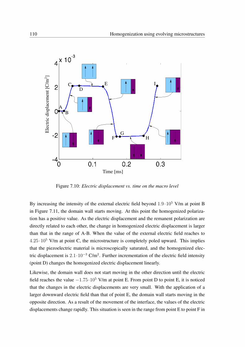
110 Homogenization using evolving microstructures
Ele
ctri
cdi
spla
cem
ent[
C/m
2]
Time [ms]
AB
CD
E
FG
H
I
Figure 7.10: Electric displacement vs. time on the macro level
By increasing the intensity of the external electric field beyond 1.9 ·105 V/m at point Bin Figure 7.11, the domain wall starts moving. At this point the homogenized polariza-tion has a positive value. As the electric displacement and the remanent polarization aredirectly related to each other, the change in homogenized electric displacement is largerthan that in the range of A-B. When the value of the external electric field reaches to4.25 ·105 V/m at point C, the microstructure is completely poled upward. This impliesthat the piezoelectric material is microscopically saturated, and the homogenized elec-tric displacement is 2.1·10−3 C/m2. Further incrementation of the electric field intensity(point D) changes the homogenized electric displacement linearly.
Likewise, the domain wall does not start moving in the other direction until the electricfield reaches the value −1.75·105 V/m at point E. From point D to point E, it is noticedthat the changes in the electric displacements are very small. With the application of alarger downward electric field than that of point E, the domain wall starts moving in theopposite direction. As a result of the movement of the interface, the values of the electricdisplacements change rapidly. This situation is seen in the range from point E to point F in
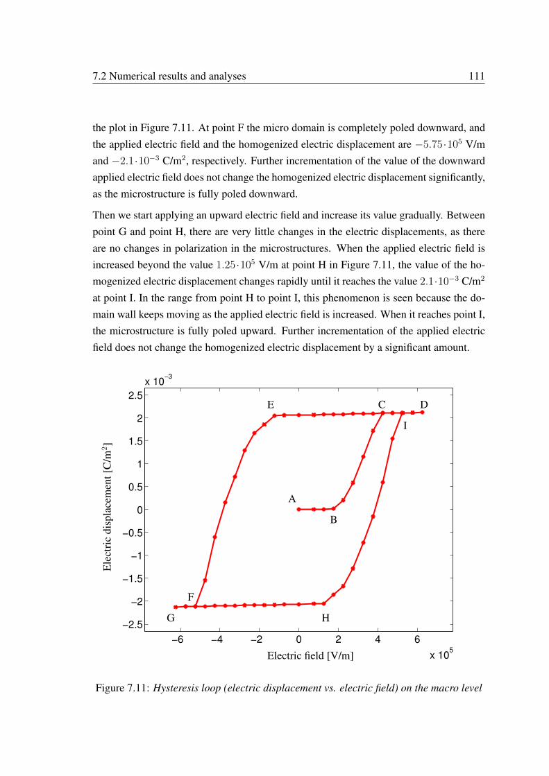
7.2 Numerical results and analyses 111
the plot in Figure 7.11. At point F the micro domain is completely poled downward, andthe applied electric field and the homogenized electric displacement are −5.75·105 V/mand −2.1·10−3 C/m2, respectively. Further incrementation of the value of the downwardapplied electric field does not change the homogenized electric displacement significantly,as the microstructure is fully poled downward.
Then we start applying an upward electric field and increase its value gradually. Betweenpoint G and point H, there are very little changes in the electric displacements, as thereare no changes in polarization in the microstructures. When the applied electric field isincreased beyond the value 1.25·105 V/m at point H in Figure 7.11, the value of the ho-mogenized electric displacement changes rapidly until it reaches the value 2.1·10−3 C/m2
at point I. In the range from point H to point I, this phenomenon is seen because the do-main wall keeps moving as the applied electric field is increased. When it reaches point I,the microstructure is fully poled upward. Further incrementation of the applied electricfield does not change the homogenized electric displacement by a significant amount.
−6 −4 −2 0 2 4 6
x 105
−2.5
−2
−1.5
−1
−0.5
0
0.5
1
1.5
2
2.5
x 10−3
Ele
ctri
cdi
spla
cem
ent[
C/m
2]
Electric field [V/m]
A
B
C DE
F
G H
I
Figure 7.11: Hysteresis loop (electric displacement vs. electric field) on the macro level
112 Homogenization using evolving microstructures
In the ranges from A to B, from C to D, from D to E, from F to G, and from G to H inFigure 7.11, very small changes in the homogenized electric displacement are observedonly due to the linear response of the dielectric effect in the material.
It should be noted that in the simulation the domain walls are not allowed to leave themicrostructures during their movement in response of the applied electric field. After thedomain is completely poled, the domain wall is kept at the element boundary.
The shape of the hysteresis loop is dependent on the time rate of the electric field. If theelectric field is changed fast, the shape of the hysteresis loop is widened, in the other caseit is narrowed.
Chapter 8
Conclusion
In this work a novel homogenization technique for piezoelectric materials is presented.Special attention is given to the homogenization of the electro-mechanical Eshelby stresstensor which is then used to determine the configurational forces at a crack tip on themacro level. A FE2-based multiscale simulation technique is adopted to accomplish thehomogenization of piezoelectric materials. In the FE2-based homogenization, three dif-ferent possible boundary conditions can be passed to the micro domain to solve the microBVP of piezoelectric materials. If the simulation is carried out with the strain tensor basedmicro boundary conditions, a problem regarding the configurational force at the crack tipoccurs. This approach does not provide a physically compatible configurational force atthe crack tip. A thorough investigation is carried out to identify and solve the problem. Itis found that this problem can be solved by using displacement gradient driven boundaryconditions on the micro domain for the mechanical part of the homogenization process. Adetailed description of boundary conditions based on displacement gradient is presented.If the micro problem is solved by strain based boundary conditions, unphysical volumeconfigurational forces occur on the macro level. It is due to the exclusion of the rotationalpart of the deformation. The displacement gradient driven boundary conditions preservethe rotational part. For this reason it results in physically compatible configurationalforces on the macro level.
For simplicity the Dirichlet boundary condition (displacement gradient driven BC formechanical part) is used for the homogenization of piezoelectric materials. Multiscalesimulations are carried out for both fixed and evolving microstructures. A macro speci-men with a horizontal sharp crack has been simulated. To obtain the effect of the micro
114 Conclusion
inhomogeneities on the crack tip configurational force at macro level, simulations areperformed with several types of microstructures containing different inhomogeneities. Itis found from the simulation results that for both horizontal and vertical polarizationsin the microstructure, a configurational force appears parallel to the crack ligament. Aconfigurational force slightly inclined to the crack ligament is noticed in the case of aninclined polarization. When the mechanical load is along the polarization of the microdomain, a lower bound is found. The case with the mechanical displacement perpendicu-lar to the polarization delivers an upper bound, because piezoelectric materials are stifferin the transverse direction to the polar axis. If an electric field along with mechanicaldisplacement is applied, the value of the configurational force reduces significantly forboth positive and negative electric fields. But the amount of the reduction is different fordifferent types of microstructures.
If an external electric field is applied to a piece of piezoelectric material, the interfacesmay move. To capture this effect of the micro heterogeneities onto the crack tip con-figurational force, the evolution of the microstructures must be considered at the time ofthe application of the external electric field. A sharp interface model is used to treat thedomain walls in piezoelectric materials, in which configurational forces are used to de-fine the kinetics of the domain wall. A simple microstructure with a 180-domain wallis considered for the homogenization process. It can be concluded from these simula-tions that the microstructures in the crack tip region are the most affected microstructures.A comparison shows that the crack tip configurational force obtained by using evolvingmicrostructures is smaller in value than that obtained by using fixed microstructures. Inthe case of evolving microstructures in piezoelectric materials, the total energy of thesystem is lowered by the motion of the interfaces of the material. As a result, a smallerconfigurational force is obtained in the case of evolving microstructures.
Simulations are carried out for the macro specimen featuring very simplified microstruc-tures, which do not represent the real situation of the microstructures of piezoelectric ma-terials. When the simulations are done with relatively complex microstructure includinggrains, the grain boundary is modeled as perfect interfaces for the sake of simplicity. Aninvestigation of the configurational force at the crack tip are only performed for mode-Itype crack. The homogenization process can be carried out in future for other types ofboundary conditions assigned to the micro domains. Further modeling of grain boundariesin piezoelectric materials can be done, and multiscale simulations can be carried out for apiezoelectric specimen including other types of crack situations, e.g., mode-II, mode-III
115
cracks. In this work multiscale simulations are done using an evolving microstructurefeaturing the simplest structure with only one interface. Further investigations can beperformed using more complex microstructures. In this case the biggest challenge willbe the tracking of the interfaces in the microstructure. For a convenient tracking of theinterfaces, the level set method may be used.

116 Conclusion
Appendix A
Appendix
A.1 Relations on a sharp interface
By defining the positive and negative interface limiting values of a scalar quantity a in thefollowing way
a+ = limε→0
a(xS + εnS),
a− = limε→0
a(xS − εnS),(A.1)
the jump JaK and average 〈〈a〉〉 of a scalar quantity a can be written as
JaK = a+ − a−,〈〈a〉〉 =
1
2(a+ + a−).
(A.2)
The jump of a product is defined by
JabK = JaK〈〈b〉〉+ 〈〈a〉〉JbK. (A.3)
According to the Lemma of Hadamard, the jump of a continuous scalar quantity a in thegradient at the singular surface S can only be in the normal direction to the surface:
JaK = 0 → J∇aK ·mγ = 0. (A.4)
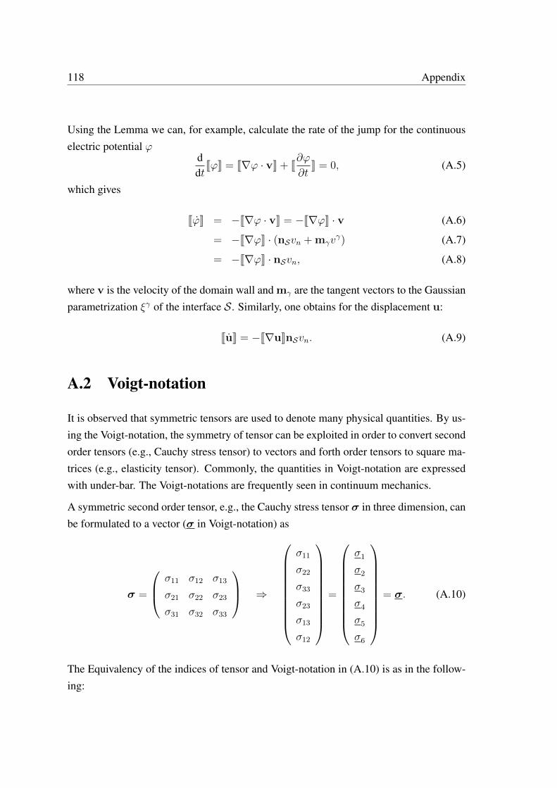
118 Appendix
Using the Lemma we can, for example, calculate the rate of the jump for the continuouselectric potential ϕ
ddt
JϕK = J∇ϕ · vK + J∂ϕ∂t
K = 0, (A.5)
which gives
JϕK = −J∇ϕ · vK = −J∇ϕK · v (A.6)
= −J∇ϕK · (nSvn + mγvγ) (A.7)
= −J∇ϕK · nSvn, (A.8)
where v is the velocity of the domain wall and mγ are the tangent vectors to the Gaussianparametrization ξγ of the interface S. Similarly, one obtains for the displacement u:
JuK = −J∇uKnSvn. (A.9)
A.2 Voigt-notation
It is observed that symmetric tensors are used to denote many physical quantities. By us-ing the Voigt-notation, the symmetry of tensor can be exploited in order to convert secondorder tensors (e.g., Cauchy stress tensor) to vectors and forth order tensors to square ma-trices (e.g., elasticity tensor). Commonly, the quantities in Voigt-notation are expressedwith under-bar. The Voigt-notations are frequently seen in continuum mechanics.
A symmetric second order tensor, e.g., the Cauchy stress tensor σ in three dimension, canbe formulated to a vector (σ in Voigt-notation) as
σ =
σ11 σ12 σ13
σ21 σ22 σ23
σ31 σ32 σ33
⇒
σ11
σ22
σ33
σ23
σ13
σ12
=
σ1
σ2
σ3
σ4
σ5
σ6
= σ. (A.10)
The Equivalency of the indices of tensor and Voigt-notation in (A.10) is as in the follow-ing:
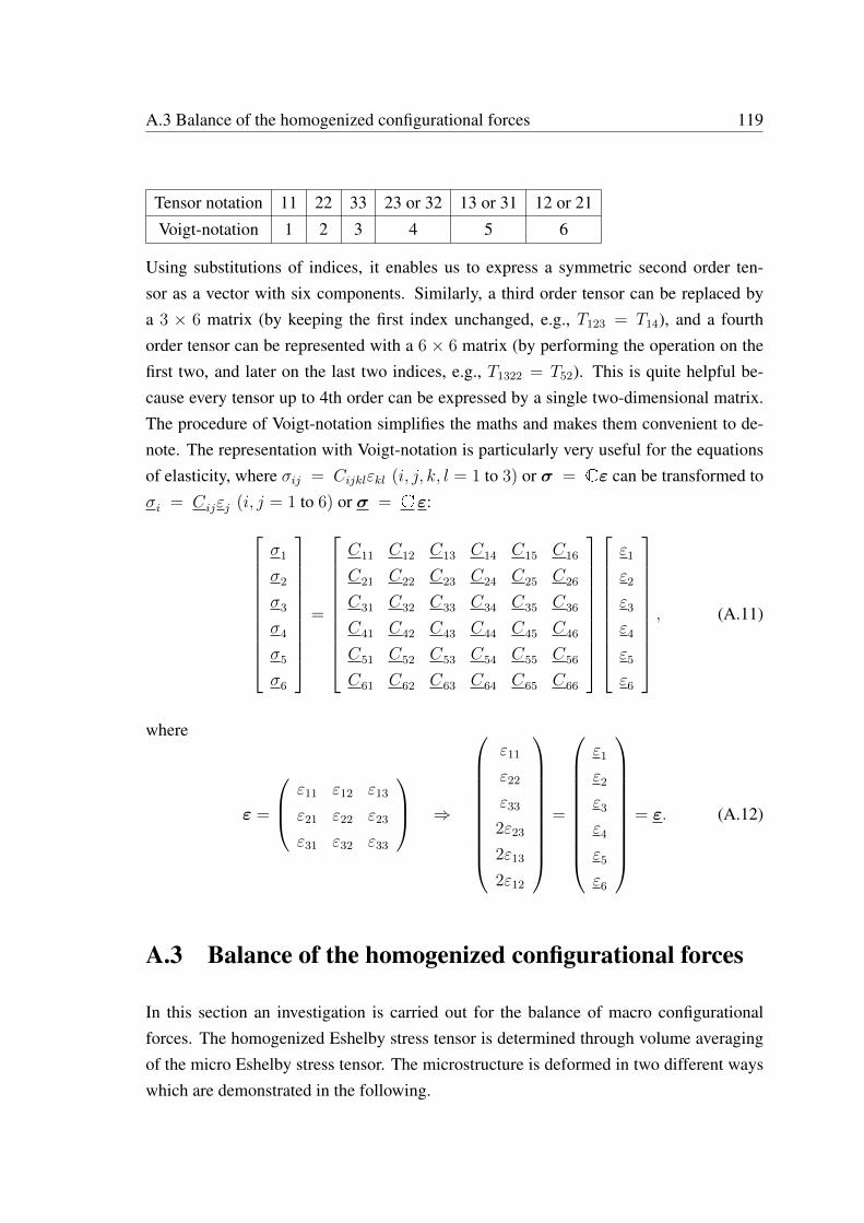
A.3 Balance of the homogenized configurational forces 119
Tensor notation 11 22 33 23 or 32 13 or 31 12 or 21
Voigt-notation 1 2 3 4 5 6
Using substitutions of indices, it enables us to express a symmetric second order ten-sor as a vector with six components. Similarly, a third order tensor can be replaced bya 3 × 6 matrix (by keeping the first index unchanged, e.g., T123 = T14), and a fourthorder tensor can be represented with a 6 × 6 matrix (by performing the operation on thefirst two, and later on the last two indices, e.g., T1322 = T52). This is quite helpful be-cause every tensor up to 4th order can be expressed by a single two-dimensional matrix.The procedure of Voigt-notation simplifies the maths and makes them convenient to de-note. The representation with Voigt-notation is particularly very useful for the equationsof elasticity, where σij = Cijklεkl (i, j, k, l = 1 to 3) or σ = Cε can be transformed toσi = Cijεj (i, j = 1 to 6) or σ = C ε:
σ1
σ2
σ3
σ4
σ5
σ6
=
C11 C12 C13 C14 C15 C16
C21 C22 C23 C24 C25 C26
C31 C32 C33 C34 C35 C36
C41 C42 C43 C44 C45 C46
C51 C52 C53 C54 C55 C56
C61 C62 C63 C64 C65 C66
ε1
ε2
ε3
ε4
ε5
ε6
, (A.11)
where
ε =
ε11 ε12 ε13
ε21 ε22 ε23
ε31 ε32 ε33
⇒
ε11
ε22
ε33
2ε23
2ε13
2ε12
=
ε1
ε2
ε3
ε4
ε5
ε6
= ε. (A.12)
A.3 Balance of the homogenized configurational forces
In this section an investigation is carried out for the balance of macro configurationalforces. The homogenized Eshelby stress tensor is determined through volume averagingof the micro Eshelby stress tensor. The microstructure is deformed in two different wayswhich are demonstrated in the following.
120 Appendix
A.3.1 Macro displacement gradient based deformation of the microdomain
The micro domain is deformed according to the macro displacement gradient for bothtypes of boundary conditions (Dirichlet and periodic boundary conditions) on the domain.By taking divergence of both sides of (5.32), we get
Σij,j =1
V
∫
Bmic
Σij,j dΩ =1
V
∫
∂Bmic
Σijnj dΓ (using divergence theorem). (A.13)
Inserting the definition of the Eshelby stress tensor in (A.13), the equation can be writtenas
Σij,j =1
V
∫
∂Bmic
(Wδij − uk,iσkj)nj dΓ
=1
V
∫
∂Bmic
δijWnj dΓ− 1
V
∫
∂Bmic
uk,iσkjnj dΓ. (A.14)
Using the definition of the displacement gradient on the boundary of the micro domainfrom equation (5.19) , equation (A.14) can be written as
Σij,j =1
V
∫
Bmic
δijW,j dΩ− 1
V
∫
∂Bmic
(uk,i + wk,i)σkjnj dΓ
=1
V
∫
Bmic
W,i dΩ− 1
V
∫
∂Bmic
uk,iσkjnj dΓ− 1
V
∫
∂Bmic
wk,iσkjnj dΓ. (A.15)
With the definition of boundary traction and using the divergence theorem, equation(A.15) can be written as
Σij,j = W,i−1
V
∫
Bmic
(uk,iσkj) ,j dΩ− 1
V
∫
∂Bmic
wk,itk dΓ
= W,i−1
V
∫
Bmic
(uk,ijσkj + uk,iσkj,j) dΩ− 1
V
∫
∂Bmic
wk,itk dΓ
= W,i−1
V
∫
Bmic
uk,ijσkj dΩ− 1
V
∫
∂Bmic
wk,itk dΓ (as σkj,j = 0). (A.16)
For periodic boundary conditions on the micro domain, it can be written that∫
∂Bmic
wk,itk dΓ =
0, as w+k,i = w−k,i and t+k = −t−k on opposite faces of the micro domain. The fluctua-
A.3 Balance of the homogenized configurational forces 121
tion term w vanishes for a Dirichlet boundary condition on the micro domain. Equation(A.16) can be written as
Σij,j = W,i−uk,ij1
V
∫
Bmic
σkj dΩ
= W,i−uk,ijσkj. (A.17)
As W,i − uk,ijσkj = gi (where gi is the macro volume configurational force), thematerial is macroscopically homogeneous, and there are no body forces in the material,there will be no macro volume configurational force in the material. Thus, equation (A.17)or the balance of homogenized configurational forces can be stated as
Σij,j = gi = 0.
In this case no unphysical volume configurational forces are produced on the macro leveldue to the homogenization of the material.
A.3.2 Macro strain based deformation of the micro domain
In this section the micro domain is deformed according to the macro strain in both typeof boundary conditions (Dirichlet and periodic boundary conditions). So, in this case thebalance of the macro configurational forces in (A.16) can written as
Σij,j =1
V
∫
Bmic
δijW,j dΩ− 1
V
∫
∂Bmic
(εki + wk,i)σkjnj dΓ
=1
V
∫
Bmic
δijW,j dΩ− 1
V
∫
∂Bmic
(uk,i − ωki + wk,i)σkjnj dΓ
=1
V
∫
Bmic
W,i dΩ− 1
V
∫
∂Bmic
uk,iσkjnj dΓ
− 1
V
∫
∂Bmic
wk,iσkjnj dΓ +1
V
∫
∂Bmic
ωkiσkjnj dΓ. (A.18)
The first three terms in (A.18) are similar as in the previous section and they will vanishin the formulation. Thus, equation (A.18) can be written as
Σij,j =1
V
∫
∂Bmic
ωkiσkjnj dΓ =1
V
∫
Bmic
(ωkiσkj) ,j dΩ =1
V
∫
Bmic
(ωki,jσkj + ωkiσkj,j) dΩ
122 Appendix
= ωki,j1
V
∫
Bmic
σkj dΩ = ωki,jσkj. (A.19)
So, the balance of the macro configurational forces can be written as
Σij,j = ωki,jσkj.
Although the material is macroscopically homogeneous and there is no macroscopic bodyforce in the material, the balance of the macro configurational forces produces some un-physical volume configurational forces. The amount of the unphysical volume configura-tional forces is −ωki,jσkj .
A.4 Domain wall driving force
A.4.1 On a 180-domain wall
The driving force acting on a 180-domain wall is approximated as illustrated in the fol-lowing. The geometry sketched in Figure 7.3(a) is considered for the formulations.
By inserting the Eshelby stress tensor of (7.2) into the domain wall driving force (firstequation in (7.5)); and assuming that there is no free charge on the domain wall (JDK ·nS = 0, where nS is the normal vector to the domain wall); and considering the me-chanical equilibrium condition on the domain wall (JσKnS = 0) , the wall driving canbe formulated as
τn = JHK− nS ·(J(∇u)TσKnS
)+ nS · (JE⊗DKnS) (A.20)
=1
2J(ε− ε0) · [C(ε− ε0)]K− J(ε− ε0) · (bTE)K
−1
2JE · (AE)K− JP0 · EK− nS ·
(J(∇u)T Kσ − JEK⊗D
)nS . (A.21)
The material parameters in equations (7.18) and (7.19) imply that the electric field is notsignificantly stronger than approximately 1 MV/m, the terms in the first line of (A.21)and the first term in the second line of (A.21) can be assumed to be small compared toJP0 ·EK. The last term in (A.21) is neglected with the same arguments, because the jumpsof (∇u)T and E in the normal direction of the domain wall are also small compared to
A.4 Domain wall driving force 123
JP0 · EK. By all the arguments and assumptions, the approximated driving force can bewritten as
τn ≈ JP0 ·EK = P0+ ·E+ −P0− ·E− =
[0
P 0
]·[
0
E2
]−[
0
−P 0
]·[
0
E2
]
= P 0E2 + P 0E2 = 2P 0E2.
A.4.2 On a 90-domain wall
Similar arguments and assumptions can be stated for a 90-domain wall of piezoelectricmaterials. This leads to the approximated driving force on a 90-domain wall
τn ≈ JP0 · EK = P0+ ·E+ −P0− ·E− =
[P 0
1
P 02
]·[
0
E2
]−[P 0
1
−P 02
]·[
0
E2
]
= P 02E2 + P 0
2E2 = 2P 02E2.

124 Appendix
Bibliography
[1] R. Ahluwalia and W. Cao. Effect of surface induced nucleation of ferroelasticdomains on polarization switching in constrained ferroelectrics. J. Appl. Phys.,93(1):537–544, 2003.
[2] R. Ahluwalia, T. Lookman, A. Saxena, and W. Cao. Domain-size dependence ofpiezoelectric properties of ferroelectrics. Phys. Rev. B, 72(1):014112, 2005.
[3] H. Allik and T. J. R. Hughes. Finite element method for piezoelectric vibration.Int. J. Numer. Meth. Eng., 2(2):151–157, 1970.
[4] G. Bao, J. W. Hutchinson, and R. M. McMeeking. Particle reinforcement of ductilematrices against plastic flow and creep. Acta Metall. Mater., 39(8):1871–1882,1991.
[5] A. Bensoussan, J.-L. Lions, and G. Papanicolau. Asymptotic analysis for periodicstructures. Studies in Mathematics and its Application, North-Holland, Amster-dam, 1978.
[6] Y. Benveniste. A new approach to the application of Mori-Tanaka’s theory in com-posite materials. MM, 6:147–157, 1987.
[7] J. Betten. Kontinuumsmechanik. Springer, Berlin, Heidelberg, New York,Barcelons, Hong Kong, London, Milan, Paris, Singapore, Tokyo, 2001.
[8] M. Braun. Configurational forces induced by finite-element discretization. Proc.Estonian Acad. Sci. Phys. Math., 46(1/2):24–31, 1997.
[9] W. Cao and G. R. Barsch. Landau-Ginzburg model of interphase boundaries inimproper ferroelastic Perovskites of D18
4h symmetry. Phys. Rev. B, 41(7):4334–4348, 1990.
[10] S. Choudhury, Y. L. Li, C. E. Krill III, and L.-Q. Chen. Phase-field simulationof polarization switching and domain evolution in ferroelectric polycrystals. ActaMater., 53(20):5313–5321, 2005.
126 BIBLIOGRAPHY
[11] S. Choudhury, Y. L. Li, C. E. Krill III, and L.-Q. Chen. Effect of grain orienta-tion and grain size on ferroelectric domain switching and evolution: phase fieldsimulations. Acta Mater., 55(4):1415–1426, 2007.
[12] T. Christman, A. Needleman, and S. Suresh. An experimental and numerical studyof deformation in metal-ceramic composites. Acta Metall., 37(11):3029–3050,1989.
[13] F. Devries, H. Dumontet, G. Duvaut, and F. Lene. Homogenization and damagefor composite structures. Int. J. Numer. Meth. Eng., 27:285–298, 1989.
[14] J. D. Eshelby. The force on an elsatic singularity. Phil. Trans. Roy. Soc. London A,244:87–112, 1951.
[15] J. D. Eshelby. The determination of the elastic field of an ellipsoidal inclusion, andrelated problems. Proc. Roy. Soc. London A, 241:376–396, 1957.
[16] J. D. Eshelby. Energy relations and the energy-momentum tensor in continummmechanics. in Kanninen, pages 77–115, 1970.
[17] F. Feyel. Multiscale FE2 elastoviscoplastic analysis of composite structures. Com-put. Mater. Sci., 16:344–354, 1999.
[18] F. Feyel. A multilevel finite element method (FE2) to describe the response ofhighly non-linear structures using generalized continua. Comput. Meth. Appl.Mech. Eng., 192:3233–3244, 2003.
[19] F. Feyel and J.-L. Chaboche. FE2 multiscale approach for modelling the elastovis-coplastic behaviour of long fiber SiC/Ti composite materials. Comput. Meth. Appl.Mech. Eng., 183:309–330, 2000.
[20] J. Fish, Q. Yu, and K.-L. Shek. Computational damage mechanics for compos-ite materials based on mathematical homogenization. Int. J. Numer. Meth. Eng.,45:1657–1679, 1999.
[21] R. B. Flippen. Domain wall dynamics in ferroelectric/ferroelastic molybdates. J.Appl. Phys., 46(3):1068–1071, 1975.
[22] P. A. Fotiu and S. Nemat-Nasser. Overall properties of elastic-viscoplastic periodiccomposites. Int. J. Plast., 12:163–190, 1996.
[23] Y. C. Fung and P. Tong. Classical and computational solid mechanics. WorldScientific, Singapore, New Jersey, London, Hong Kong, 2001.
[24] M. G. D. Geers, V. G. Kouznetsova, and W. A. M. Brekelmans. Multi-scalecomputational homogenization: Trends and challenges. J. Comput. Appl. Math.,234:2175–2182, 2010.
BIBLIOGRAPHY 127
[25] S. Ghosh, K. Lee, and S. Moorthy. Multiple scale analysis of heterogeneous elasticstructures using homogenization theory and Voronoi cell finite element method.Int. J. Sol. Struc., 32(1):27–62, 1995.
[26] S. Ghosh, K. Lee, and S. Moorthy. Two scale analysis of heterogeneous elastic-plastic materials with asymptotic homogenization and Voronoi cell finite elementmodel. Comput. Meth. Appl. Mech. Eng., 132, 1996.
[27] S. Ghosh, K. Lee, and S. Moorthy. A multi-level computational model for multi-scale damage analysis in composite and porous materials. Int. J. Sol. Struc., 38,2001.
[28] O. Goy. Point defects in piezoelectric materials – continuum mechanical modellingand numerical simulation. PhD thesis, Technische Universität Kaiserslautern,Kaiserslautern, 2010.
[29] D. Gross and T. Seelig. Bruchmechanik: Mit einer Einführung in dieMikromechanik. Springer, Berlin, 2007.
[30] J. M. Guedes and N. Kikuchi. Preprocessing and postprocessing for materials basedon the homogenization method with adaptive finite element methods. Comput.Meth. Appl. Mech. Eng., 83:143–198, 1990.
[31] M. E. Gurtin. An introduction to continuum mechanics. Academic Press, NewYork, London, Toronto, Sydney, San Francisco, 1981.
[32] M. E. Gurtin. Configurational forces as basic concepts of continuum physics.Springer, New York, Berlin, Heidelberg, 2000.
[33] Z. Hashin. The elastic moduli of heterogeneous materials. J. Appl. Mech., 29:143–150, 1962.
[34] Z. Hashin. Analysis of composite materials - a survey. J. Appl. Mech., 50:481–505,1983.
[35] Z. Hashin and A. Shtrikman. A variational approach to the theory of the elasticbehaviour of polycristals. J. Mech. Phys. Solid., 10:343–352, 1962.
[36] Z. Hashin and A. Shtrikman. On some variational principles in anisotropic andnonhomogeneous elasticity. J. Mech. Phys. Solid., 10:335–342, 1962.
[37] Z. Hashin and A. Shtrikman. A variational approach to the theory of the elasticbehaviour of multiphase materials. J. Mech. Phys. Solid., 11:127–140, 1963.
[38] P. Haupt. Continuum mechanics and theory of materials. Springer, Heidelberg,New York, Barcelona, Hong Kong, London, Milan, Paris, Singapure, Tokyo, 2000.
128 BIBLIOGRAPHY
[39] R. Hill. A self-consistent mechanics of composite materials. J. Mech. Phys. Solid.,13:213–222, 1965.
[40] G. A. Holzapfel. Nonlinear solid mechanics: a continuum approach for engineer-ing. John Wiley & Sons, Chichester, 2001.
[41] T. J. R. Hughes. The finite element method. Prentice Hall, Englewood Cliffs, 1987.
[42] J. D. Jackson. Classical electrodynamics, 3rd edition. John Wiley & Sons, Inc.,New York, 1999.
[43] P. Kanouté, D. P. Boso, J. L. Chaboche, and B. A. Schrefler. Multiscale methodsfor composites: a review. Arch. Comput. Meth. Eng., 16:31–75, 2009.
[44] M.-A. Keip and J. Schröder. Effective electromechanical properties of heteroge-neous piezoelectrics. Advances in Extended and Multifield Theories for Continua,Lecture Notes in Applied and Computational Mechanics, 59:109–128, 2011.
[45] H. Kessler and H. Balke. A continuum analysis of charge induced ferroelectricdomain wall motions. J. Mech. Phys. Solids, 54(1):86–112, 2006.
[46] H. Kessler and H. Balke. A continuum analysis of the driving forces of ferroelec-tric/ferroelastic domain wall motions. J. Mech. Phys. Solids, 54(1):113–127, 2006.
[47] M. Khalaquzzaman, B. X. Xu, S. Ricker, and R. Müller. Computational homog-enization of piezoelectric materials using FE2 to determine configurational forces.Technische Mechanik, 32(1):21–37, 2012.
[48] R. Kienzler and G. Herrmann. Mechanics in material space. Springer, New York,Berlin, Heidelberg, 2000.
[49] V. Kouznetsova, W. A. M. Brekelmans, and F. P. T. Baaijens. An approach to micro-macro modeling of heterogeneous materials. Comput. Mech., 27:37–48, 2001.
[50] E. Kröner. Berechnung der elastichen Konstanten des Vielkristalls aus den Kon-stanten des Einkristalls. Z. Phys., 151:504–518, 1958.
[51] L. D. Landau and E. M. Lifshitz. The classical theory of fields, vol. 2 of courseof theoretical physics, 4th edition. Butterworth-Heinemann, Amsterdam, Boston,Heidelberg, 1980.
[52] L. D. Landau and E. M. Lifshitz. Electrodynamics of continuous media, vol. 8 ofcourse of theoretical physics, 2nd edition. Butterworth-Heinemann, Amsterdam,Boston, Heidelberg, 1984.
[53] P. H. Leo and R. F. Sekerka. The effect of surface stress on crystal-melt and crystal-crystal equilibrium. Acta Metall., 37(12):3119–3138, 1989.
BIBLIOGRAPHY 129
[54] Z. Li, C. Wang, and C. Chen. Effective electromechanical properties of transverselyisotropic piezoelectric ceramics with microvoids. Comput. Mater. Sci., 27:381–392, 2003.
[55] I.-S. Liu. Continuum mechanics. Springer, Berlin, Heidelberg, New York,Barcelons, Hong Kong, London, Milan, Paris, Singapore, Tokyo, 2002.
[56] R. E. Loge and Z. Suo. Nonequilibrium thermodynamics of ferroelectric domainevolution. Acta Mater., 44(8):3429–3438, 1996.
[57] J. E. Marsden and T. J.R. Hughes. Mathematical foundations of elasticity. Devor,Mineola, New York, 1983.
[58] G. A. Maugin. Configurational forces: thermomechanics, physics, mathematics,and numerics. Chapman & Hall/CRC, London, Glasgow, New York, Tokyo, Mel-bourne, Madras, 2010.
[59] P. E. McHugh, R. J. Asaro, and C. F. Shih. Computational modeling of metalmatrix composite materials - II. isothermal stress-strain behaviour. Acta Metall.Mater., 41(5):1477–1488, 1993.
[60] R. McMeeking and A. Ricoeur. The weight function for cracks in piezoelectrics.Int. J. Solid Struc., 40:6143–6162, 2003.
[61] V. Mehling. Phenomenological modeling of ferroelectric material behavior. PhDthesis, Technische Universität Darmstadt, Darmstadt, 2007.
[62] J. C. Michel, H. Moulinec, and P. Suquet. Effective properties of composite mate-rials with periodic microstructure: a computational approach. Comput. Meth. Appl.Mech. Eng., 172:109–143, 1999.
[63] C. Miehe. Strain-driven homogenization of inelastic microstructures and compos-ites based on an incremental variational formulation. Int. J. Numer. Meth. Eng.,55:1285–1322, 2002.
[64] C. Miehe. Computational micro-to-macro transitions for discretized micro-structures of heterogeneous materials at finite strains based on the minimizationof averaged incremental energy. Comput. Meth. Appl. Mech. Eng., 192:559–591,2003.
[65] C. Miehe and A. Koch. Computational micro-to-macro transitions of discretizedmicrostructures undergoing small strains. Arch. Appl. Mech., 72:300–317, 2002.
[66] C. Miehe, J. Schotte, and J. Schröder. Computational micro-macro transitions andoverall moduli in the analysis of polycrystals at large strains. Comput. Mater. Sci.,16:372–382, 1999.
130 BIBLIOGRAPHY
[67] C. Miehe, J. Schröder, and J. Schotte. Computational homogenization analysis infinite plasticity. Simulation of texture development polycrystalline materials. Com-put. Meth. Appl. Mech. Eng., 171:387–418, 1999.
[68] T. Mori and K. Tanaka. Average stress in matrix and average elastic energy ofmaterials with misfitting inclusions. Acta Metall., 21:571–574, 1973.
[69] H. Moulinec and P. Suquet. A numerical method for computing the overall re-sponse of nonlinear composites with complex microstructure. Comput. Meth. Appl.Mech. Eng., 157:69–94, 1998.
[70] R. Müller and D. Gross. 3D simulation of equilibrium morphologies of precipitates.Comput. Mater. Sci., 11:35–44, 1998.
[71] R. Müller and D. Gross. 3D inhomogeneous, misfitting second phage particles-equilibrium shapes and morphological development. Comput. Mater. Sci., 16:53–60, 1999.
[72] R. Müller, D. Gross, and D. C. Lupascu. Driving forces on domain walls in fer-roelectric materials and interaction with defects. Comput. Mater. Sci., 35:42–52,2006.
[73] R. Müller, S. Kolling, and G. A. Maugin. On configurational forces in the contextof the finite element method. Int. J. Numer. Meth. Eng., 53(7):1557–1575, 2002.
[74] R. Müller and G. A. Maugin. On material forces and finite element discretizations.Comput. Mech., 29(1):52–60, 2002.
[75] T. Nakamura and S. Suresh. Effect of thermal residual stress and fiber packing ondeformation of metal-matrix composites. Acta Metall. Mater., 41(6):1665–1681,1993.
[76] S. Nemat-Nasser and M. Hori. Micromechanics: overall properties of heteroge-neous materials. North-Holland, Amsterdam, London, New York, Tokyo, 1993.
[77] R. Ogden. Non-linear elastic deformations. Dover Publications, Inc., Mineola,New York, 1984.
[78] C. Poizat and M. Sester. Effective properties of composites with embedded piezo-electric fibres. Comput. Mater. Sci., 16:89–97, 1999.
[79] E. M. Purcell. Electricity and magnetism, vol. 2 of Berkley physics course.McGraw-Hill, Inc., New York, 1965.
[80] Q. Qin. Fracture mechanics of piezoelectric materials. WIT Press, Southamton,2001.
BIBLIOGRAPHY 131
[81] A. Reuss. Berechnung der Fliessgrenze von Mischkristallen auf Grund der Plastiz-itätsbedingung für Einkristalle. Z. Angew. Math. Mech., 9:49–58, 1929.
[82] J. R. Rice. A path independent integral and the approximate analysis of strainconcentration by notches and cracks. J. Appl. Mech., 35:379–386, 1968.
[83] S. Ricker, J. Mergheim, and P. Steinmann. On the scale computation of defectdriving force. Int. J. Multiscale Comput. Eng., 7(5):457–474, 2009.
[84] S. Ricker, J. Mergheim, P. Steinmann, and R. Müller. A comparison of differentapproaches in the multi-scale computation of configurational forces. Int. J. Frac.,166(1-2):203–214, 2010.
[85] E. Sanchez-Palenzia. Non-homogeneous media and vibration theory. Lecture Notesin Physics, 127:193–278, 1980.
[86] D. Schrade. Microstructural modeling of ferroelectric material behavior. PhDthesis, Technische Universität Kaiserslautern, Kaiserslautern, 2011.
[87] D. Schrade, R. Müller, and D. Gross. Parameter identification in phase field modelsfor ferroelectrics. Proc. Appl. Math. Mech., 9(1):369–370, 2009.
[88] D. Schrade, R. Müller, D. Gross, T. Utschig, V. Y. Shur, and D. C. Lupascu. In-teraction of domain walls with defects in ferroelectric materials. Mech. Mater.,39:161–174, 2007.
[89] D. Schrade, R. Müller, B. X. Xu, and D. Gross. Domain evolution in ferroelec-tric materials: a continuum phase field model and finite element implementation.Comput. Meth. Appl. Mech. Eng., 196(41-44):4365–4374, 2007.
[90] D. Schrade, B. X. Xu, R. Müller, and D. Gross. On phase field modeling of ferro-electrics: parameter indication and verification. ASME conf. proc. (Smart Materi-als, Adaptive Structures and Intelligent Sytems 2008, 1:299–306, 2008.
[91] J. Schröder. Derivation of the localization and homogenization conditions forelectro-mechanically coupled problems. Comp. Mater. Sci., 46:595–599, 2009.
[92] J. Schröder and M.-A. Keip. A framework for the two-scale homogenization ofelectro-mechanically coupled boundary value problems, advanced structured ma-terials (1): computer methods in mechanics. Springer, 2010.
[93] J. Schröder and M.-A. Keip. Multiscale modeling of electro-mechanically coupledmaterials: homogenization procedure and computation of overall moduli. IUTAMSymposium on Multiscale Modelling of Fatigue, Damage and Fracture in SmartMaterials, 24 of IUTAM Bookseries:265–276, 2011.
[94] J. Schröder and M.-A. Keip. Two-scale homogenization of electro-mechanicallycoupled boundary value problems. Comput. Mech., 50:229–244, 2012.
132 BIBLIOGRAPHY
[95] V. Y. Shur, A. L. Gruverman, V. P. Kuminov, and N. A. Tonkachyova. Dynamics ofplane domain walls in lead germanate and gadolinium molybdate. Ferroelectrics,111(1):197–206, 1990.
[96] V. Y. Shur, A. L. Gruverman, V. P. Kuminov, and N. A. Tonkachyova. Dynamicsof incoherent domain walls in gadolinium molybdate. Ferroelectrics, 130(1):341–346, 1992.
[97] V. Y. Shur, E. V. Nikolaeva, E. L. Rumyantsev, E. I. Shishkin, A. L. Subbotin, andV. L. Kozhevnikov. Smooth and jump-like dynamics of the plane domain wall ingadolinium molybdate. Ferroelectrics, 222(1):323–331, 1999.
[98] R. J. M. Smit, W. A. M. Brekelmans, and H. E. H. Meijer. Prediction of the me-chanical behaviour of non-linear heterogeneous systems by multi-level finite ele-ment modeling. Comput. Meth. Appl. Mech. Eng., 155:181–192, 1998.
[99] Y. Su and C. M. Landis. Continuum thermodynamics of ferroelectric domain evo-lution: theory, finite element implementation, and application to domain wall pin-ning. J. Mech. Phys. Solid., 55(2):280–305, 2007.
[100] P. M. Suquet. Local and global aspects in the mathematical theory of plasticity.In S. Sawczuk and G. Bianchi, editors, Plasticity today: Modelling, Methods andApplications, pages 279-310, Elsevier, London, 1985.
[101] S. Suresh, A. Mortensen, and A. Needleman. Fundamentals of metal-matrix com-posites. Butterworth-Heinemann, Boston, 1993.
[102] K. Tanaka and T. Mori. Note on volume integrals of the elastic field around anellipsoidal inclusion. J. Elasticity, 2:199–200, 1972.
[103] A. Teledano and H. Murakami. A high order mixture model for periodic particulatecomposites. Int. J. Solid Struc., 23:989–1002, 1987.
[104] K. Terada and N. Kikuchi. Nonlinear homogenization method for practical appli-cations. In Ghosh, S. and Ostoja-Starzewski, M., editors, Computational methodsin micromechanics, AMD-Vol. 212/Md-Vol. 62, pages 1-16. ASME, 1995.
[105] K. Terada and N. Kikuchi. A class of general algorithms for multi-scale analysisof heterogeneous media. Comput. Meth. Appl. Mech. Eng., 190:5427–5464, 2001.
[106] M. Toda, S. Tosima, E. Shima, and T. Iwasa. Variable delay devices using fer-roelastic and ferroelectric crystal Gd2(MoO4)3. IEEE Transaction on Sonics andUltrasonics, SU-20(4):376–379, 1973.
[107] W. Voigt. Über the Beziehung zwischen den Elastizitätskonstanten isotroper Kör-per. Wied. Ann., 38:573–587, 1889.
BIBLIOGRAPHY 133
[108] J. Wang and M. Kamlah. Domain structures of ferroelectric nanotubes controlledby surface charge compensation. Appl. Phys. Lett., 93(4):042906, 2008.
[109] J. Wang, S.-Q. Shi, L.-Q. Chen, Y. Li, and T.-Y. Zhang. Phase-field simulationsof ferroelectric/ferroelastic polarization switching. Acta Mater., 52(3):749–764,2004.
[110] J. R. Willis. Bounds and self-consistent estimates for the overall properties ofanisotropic composites. J. Mech. Phys. Solid., 25:185–202, 1977.
[111] P. Wriggers. Nichtlineare Finite-Element-Methoden. Springer, Berlin, 2001.
[112] Y. Xu. Ferroelectric materials and their applications. Elsevier Science PublishersB.V., Holland, 1991.
[113] W. Zhang and K. Bhattacharya. A computational model of ferroelectric domains.Part I: model formulation and domain switching. Acta Mater., 53(1):185–198,2005.
[114] O. C. Zienkiewicz and R. L. Taylor. The finite element method, the basis (volume1). Butterworth-Heinemann, Oxford, 2000.

Lebenslauf
Name: Khalaquzzaman, Md
----------------------------------------------------------------------------------------------------------------
01/1983 - 04/1993 Secondary School Certificate Examination,Rajshahi, Bangladesch
07/1993 - 08/1995 Higher Secondary Certificate Examination,Dhaka, Bangladesch
12/1996 - 04/2002 Bachelorstudium im Bauingenieurwesen, BangladeshUniversity of Engineering and Technology,Dhaka, BangladeschAbschluss: Bachelor im Bauingenieurwesen
10/2003 - 09/2009 Masterstudium im Computational Sciences inEngineering, TU BraunschweigAbschluss: Master im CSE
10/2009 – 03/2012 Stipendiat im DFG-Graduiertenkolleg 814,Lehrstuhl für Technische Mechanik,Technische Universität Kaiserslautern
04/2012 – 11/2012 Stipendiat der TU Kaiserslautern,Lehrstuhl für Technische Mechanik
12/2012 – 11/2013 Wissenschaftlicher Mitarbeiter,Lehrstuhl für Technische Mechanik,Technische Universität Kaiserslautern