Homogenization of thin piezoelectric perforated shells · HOMOGENIZATION OF THIN PIEZOELECTRIC PERFORATED SHELLS 877 The shell with thickness 2 t and middle surface S is de ned by

ESAIM: M2AN ESAIM: Mathematical Modelling and Numerical AnalysisVol. 41, No 5, 2007, pp. 875–895 www.esaim-m2an.orgDOI: 10.1051/m2an:2007046

HOMOGENIZATION OF THIN PIEZOELECTRIC PERFORATED SHELLS

Marius Ghergu1, Georges Griso

2, Houari Mechkour

3and Bernadette Miara

4

Abstract. We rigorously establish the existence of the limit homogeneous constitutive law of a piezo-electric composite made of periodically perforated microstructures and whose reference configurationis a thin shell with fixed thickness. We deal with an extension of the Koiter shell model in which thethree curvilinear coordinates of the elastic displacement field and the electric potential are coupled.By letting the size of the microstructure going to zero and by using the periodic unfolding methodcombined with the Korn’s inequality in perforated domains, we obtain the limit model.

Mathematics Subject Classification. 74K25, 74Q05, 35B27.

Received October 21, 2006. Revised March 18, 2007.

1. Introduction

The homogenization method used in the modelling of periodically structured domains has been extensivelydeveloped after the pioneering work (with a mathematical point of view) of Bensoussan et al. [3]. A rigorousasymptotic study is given in Nguetseng [20], Allaire [1], Sanchez-Hubert and Sanchez-Palencia [22, 23], Cio-ranescu and Donato [8] and in Cioranescu and Saint-Jean Paulin [10] in the case of thin perforated domains.The approach we use in this paper differs from these quoted before and is more similar to the periodic modula-tion method found in [2, 17]; it relies on the periodic unfolding method introduced by Cioranescu et al. [7] andrecently also extended to perforated domains [9].

The Koiter’s model for elastic shells combines the effects of the two tensors: the membrane tensor and theflexural tensor. An asymptotic behavior of the displacement field in case of composite or laminated elastic shellsis described, for example, in Caillerie and Sanchez-Palencia [5] or Lewinski and Telega [16]. The coupling, in theKoiter model of the two-dimensional linearized change of metric and curvature tensors which present differentorder of derivatives of the curvilinear coordinates of the elastic displacement field gives rise to local problemsof different nature than the global one; in our paper these problems can be found in equations (30)–(32) andequations (34) respectively. Another interesting extension is due to Caillerie and Sanchez-Palencia [6] when

Keywords and phrases. Computational solid mechanics, homogenization, perforations, piezoelectricity, shells.

1 Institute of Mathematics “Simion Stoilow” of the Romanian Academy, PO Box 1-764, RO-014700, Bucharest, [email protected] Laboratoire Jacques-Louis Lions, Universite Pierre et Marie Curie (Paris VI), 4 Place Jussieu, 75252 Paris, [email protected] Ecole Polytechnique, Centre de Mathematiques Appliquees, CMAP (CNRS UMR 7641), 91128 Palaiseau, [email protected] Laboratoire de Modelisation et Simulation Numerique, ESIEE, 2 Boulevard Blaise Pascal, 91360 Noisy-Le-Grand, [email protected]

c© EDP Sciences, SMAI 2007

Article published by EDP Sciences and available at http://www.esaim-m2an.org or http://dx.doi.org/10.1051/m2an:2007046

http://www.edpsciences.org

http://www.esaim-m2an.org

http://dx.doi.org/10.1051/m2an:2007046

876 M. GHERGU ET AL.

the size of each microstructure is comparable with its thickness; this approach will be addressed later in ourframework of piezoelectric material.

In the piezoelectric effect there exists a coupling between elastic field and electric field, i.e., under an appliedmechanical force a piezoelectric body undergoes a strain that produces an electric field and conversely an appliedelectric field produces a mechanical stress. Many cristalline materials (such as quartz, Rochelle salt) or ceramicmaterials (barium titanate, lead zirconate titanate) exhibit a piezoelectric behavior. Also human skin and humanbone present this property but with a very low elastic-electric coupling efficiency. These materials are used assensors or actuators, ultrasonic or shear transducers. For a more complete study of piezoelectric materials werefer the reader to Dieulesaint and Royer [12] or Ikeda [14]. The modelling of laminated three-dimensionalpiezoelectric composite has already been analyzed by Bourgeat et al. [4] and Mechkour [18].

Having in mind such applications as [21] (which presents a piezoelectric porous electrode used as a spatial filtersensor) or [19] (which presents a bio-material made of a piezoelectric matrix with elastic inclusions of osteoblastsand used as a micro device supposed to improve the bone regeneration) our purpose in this paper is to combinethe different previous features: shell structure, perforations and piezoelectric model to mathematically analyzea well adapted model. Hence we study the homogenization of a thin shell having periodically distributedmicrostructures with small size ε, each microstructure containing a hole. The shell is assumed to be of constantthickness and periodicity, in this case, is viewed as periodicity with respect to the curvilinear parametrizationof its middle surface. The question we address here is to establish the limit model obtained when ε goes to zero.

The paper is organized as follows. In Section 2 we introduce the elements of differential geometry necessaryto describe the geometry of the shell, we recall the two-dimensional constitutive law of a piezoelectric material(Eq. (4)) and the elastic-electric equilibrium equations of periodically perforated structures (Eq. (8)). In Sec-tion 3 we recall the definition and main properties of the unfolding operator T ε associated to a reference cell.Finally, in Section 4, we use the operator T ε as a tool to establish the strong convergence of the three covariantcomponents of the displacement field and of the electric potential (Eq. (19)) and therefore to obtain the limitmodel (Eq. (34)); moreover a strong convergence is established for the correctors (Eq. (45)). For the sake ofclarity the delicate proof of Korn’s inequality for shells in perforated domain is postponed to the Appendix.

2. Two-dimensional model of shell

2.1. Reference configuration

We denote1 by xα the coordinates of a point x ∈ R2, and by ∂α := ∂/∂xα the derivative with respect to xα.

Let Ω ⊂ R2 be a smooth, connex domain with C2 boundary. The shell with middle surface S is defined with the

aid of a one-to-one mapping θ ∈ C3(Ω) with S = θ(Ω). We assume that for all x = (x1, x2) ∈ Ω, the two vectorsaα(x) := ∂αθ(x) are linearly independent. Hence, the vectors aα(x) span the tangent plane to the surface atthe point θ(x) ∈ S, x ∈ Ω. Let a3(x) be the unit normal vector to S at θ(x) defined by

a3(x) =a1(x) × a2(x)|a1(x) × a2(x)|

·

The three vectors ai(x) form the covariant basis at θ(x) while the three vectors ai(x) given by relations

ai(x) · aj(x) = δij,

form the two dimensional contravariant basis at θ(x). Let us remark that the vectors aα(x) defined above alsospan the tangent plane to S at θ(x) and that a3(x) = a3(x). Let aαβ = aα · aβ and aαβ = aα · aβ be thecovariant and the contravariant components of the metric tensor of S. The area element along the surface S is√a dx1 dx2 where a = det(aαβ).

1Throughout this paper, Latin indices and exponents take their values in the set 1, 2, 3, Greek indices and exponents (except ε)take their values in the set 1, 2 and the summation convention with respect to repeated indices and exponents is used. Boldfaceletters represent vector-valued functions or spaces.

HOMOGENIZATION OF THIN PIEZOELECTRIC PERFORATED SHELLS 877

The shell with thickness 2t and middle surface S is defined by the map

Θ : Ωt := Ω × [−t, t] → R3,

Θ(x1, x2, x3) = θ(x1, x2) + x3a3(x1, x2), for all (x1, x2, x3) ∈ Ωt.

For t > 0 small enough, the mapping Θ is injective and the three vectors gi(x1, x2, x3) = ∂iΘ(x1, x2, x3) arelinearly independent at each point (x1, x2, x3) ∈ Ωt. The vectors gi(x1, x2, x3) form the three dimensionalcovariant basis at the point Θ(x1, x2, x3). In this way we have defined a shell having the middle surface S andconstant thickness 2t > 0, i.e., a body whose reference configuration is the set Θ(Ωt).

2.2. Three-dimensional piezoelectricity

Under the action of applied volume loading f ∈ L2(Ωt) and without electric charges, the shell undergoes anelastic displacement field u and a scalar electric potential ϕ given by the equations below:

−div σ(u, ϕ) = f in Ωt,

−div D(u, ϕ) = 0 in Ωt,(1)

where σ = (σij) is the linearized stress tensor and D = (Di) is the electric displacements vector defined asσij(u, ϕ) = cijklskl(u) + ekij∂kϕ,

Di(u, ϕ) = − eiklskl(u) + dij∂jϕ,(2)

and (div σ(Bu,ϕ))j = ∂iσ

ij(u, ϕ),

div D(u, ϕ) = ∂iDi(u, ϕ),

here (sij) represents the linearized deformation tensor which is given by

sij(u) =12(∂iuj + ∂jui).

Hence, the characteristics of the three dimensional piezoelectric material are given by the elastic tensor (cijkl),the dielectric tensor (dij) and the piezoelectric coupling tensor (eijk). These three tensors have the followingproperties:

• the elastic tensor (cijkl) is symmetric and positive definite, that is,

cijkl = cjikl = cklij ,

and there exists αc > 0 such that cijklXijXkl ≥ αcXijXij , ∀Xij = Xji ∈ R;• the dielectric tensor (dij) is symmetric and positive definite, that is, dij = dji, and there exists αd > 0

such that dijXiXj ≥ αdXiXi, ∀X = (Xi) ∈ R3;

• the piezoelectric tensor (eijl) is symmetric in the sense that eijk = ejik .We assume that the components of the the above three tensors belong to L∞(Ωt).The variational formulation of the problem (1) reads: find u ∈ H1

0 (Ωt; R3) and ϕ ∈ H10 (Ωt) such that⎧⎪⎪⎨⎪⎪⎩

∫Ωt

(c(u,v) + e(v, ϕ))dx =∫

Ωt

f · v dx ∀v ∈ H10 (Ωt; R3),∫

Ωt

(−e(u, ψ) + d(ϕ, ψ))dx = 0 ∀ψ ∈ H10 (Ωt),

(3)


where c, e and d are given by ⎧⎨⎩ c(u,v) = cijklsij(u)skl(v),e(v, ψ) = eijksij(v)∂kψ,d(ϕ, ψ) = dij∂iϕ ∂jψ.

2.3. From three-dimensional equations to two-dimensional equations:the piezoelectric shell equations

In the case of two-dimensional model of piezoelectric shell, four new tensors are needed. Their expressionsin terms of the previous three dimensional ones are given in Haenel [13], equations 3.2.23, 3.2.27:

• the membrane elastic tensor (cαβστM ), which is symmetric and positive definite;

• the flexural elastic tensor (cαβστF ), which is symmetric and positive definite;

• the dielectric tensor (dαβ), which is symmetric and positive definite;• the piezoelectric tensor (eαβσ), which is symmetric in the sense that eαβσ = eβασ.

With previous assumptions, we deduce that the components of the four above tensors belong to L∞(Ω).We consider a shell in curvilinear coordinates inspired by a Koiter model for the elastic shells (see [15])

in which the relation between the membrane constraints Tαβ, the bending constraints Mαβ and the electricdisplacements Dσ are expressed in terms of the three covariant components u = (ui) of the elastic displacementaiui and of the electric potential ϕ as follows:⎧⎪⎪⎨⎪⎪⎩

Tαβ(u, ϕ) = cαβστM γστ (u) + eαβσ∂σϕ,

Mαβ(u, ϕ) = − cαβστF ρστ (u),

Dσ(u, ϕ) = − eαβσγαβ(u) + dστ∂τϕ.

(4)

In relations (4), the tensor γ = (γαβ) represents the two-dimensional linearized change of metric tensor. Itscomponents are given by

γαβ(v) =12(∂αvβ + ∂βvα) − Γσ

αβvσ − bαβv3. (5)

Also in relations (4), ρ = (ραβ) denotes the two-dimensional linearized change of curvature tensor. Its compo-nents are given by

ραβ(v) = ∂2αβv3 − Γσ

αβ∂σv3 − bσαbσβv3 + bσα∂βvσ + bσβ∂αvσ + (∂βbσα − bταΓσ

βτ − bτβΓσατ )vσ, (6)

where bαβ , bβα represent the covariant and the contravariant components of the curvature tensor of the surface S,they are given by

bαβ = a3 · ∂αaβ, bβα = a3 · ∂αaβ .

In (5)–(6), (Γσαβ) denote the two-dimensional Christoffel symbols for the surface S, that is, Γσ

αβ = aσ · ∂αaβ .On the boundary ∂Ω we assume that the elastic dispacement field u and the electric potential ϕ verify an

homogeneous Dirichlet condition, u = 0 and ϕ = 0 on ∂Ω.Assume that the resultant of the applied mechanics forces p expressed in terms of the mean value of f in the

covariant basis satisfies the regularity condition p ∈ L2(Ω) and set V (Ω) = H10 (Ω) ×H1

0 (Ω) × H20 (Ω). Then,

the couple (u, ϕ) ∈ V (Ω) ×H10 (Ω) is the unique solution of the variational problem (see Haenel [13]):⎧⎪⎪⎨⎪⎪⎩

∫Ω

(cK(u,v) + eK(v, ϕ))√adx =

∫Ω

p · v√a dx ∀v ∈ V (Ω),∫

Ω

(−eK(u, ψ) + dK(ϕ, ψ))√adx = 0 ∀ψ ∈ H1

0 (Ω),(7)


YT

*

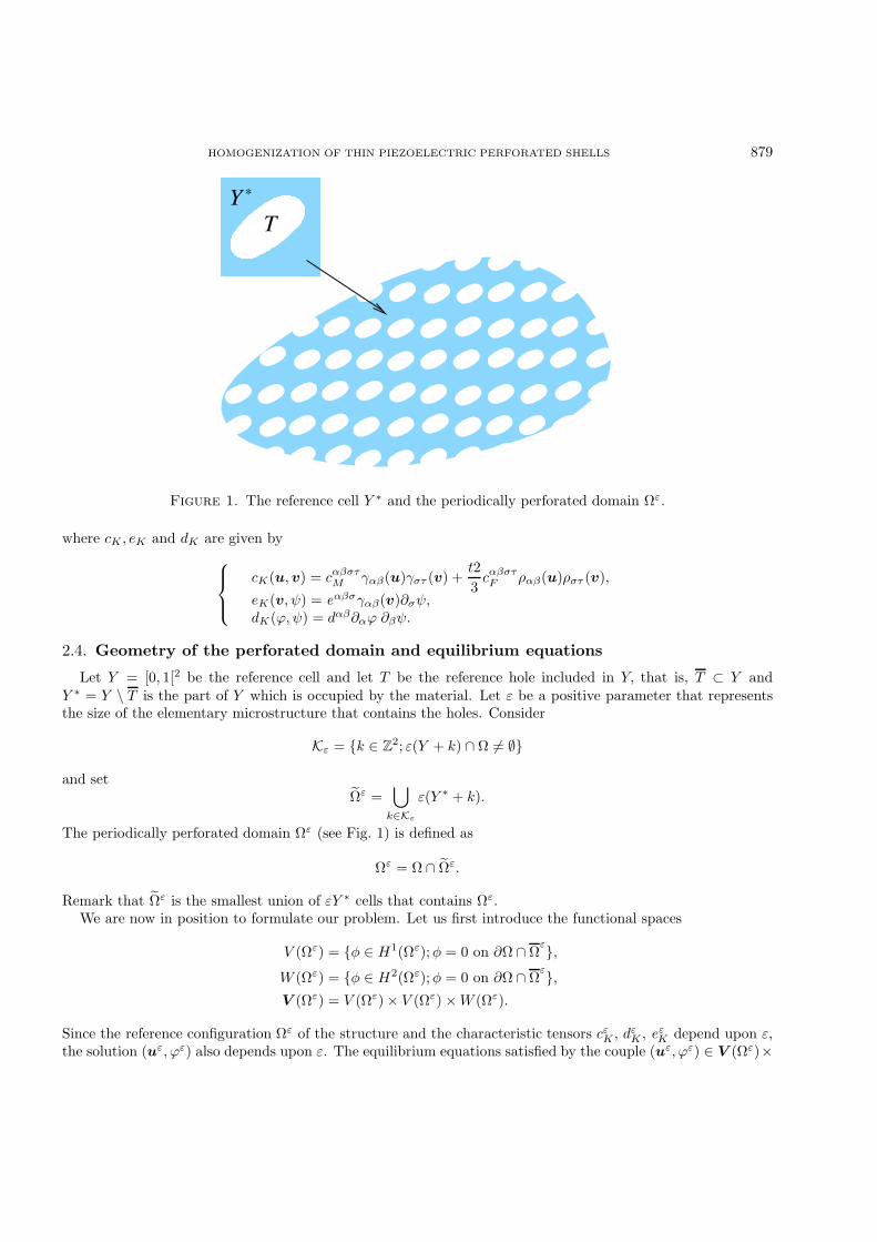
Figure 1. The reference cell Y ∗ and the periodically perforated domain Ωε.

where cK , eK and dK are given by⎧⎪⎨⎪⎩cK(u,v) = cαβστ

M γαβ(u)γστ (v) +t23cαβστF ραβ(u)ρστ (v),

eK(v, ψ) = eαβσγαβ(v)∂σψ,dK(ϕ, ψ) = dαβ∂αϕ ∂βψ.

2.4. Geometry of the perforated domain and equilibrium equations

Let Y = [0, 1[2 be the reference cell and let T be the reference hole included in Y, that is, T ⊂ Y andY ∗ = Y \ T is the part of Y which is occupied by the material. Let ε be a positive parameter that representsthe size of the elementary microstructure that contains the holes. Consider

Kε = k ∈ Z2; ε(Y + k) ∩ Ω = ∅

and setΩε =

⋃k∈Kε

ε(Y ∗ + k).

The periodically perforated domain Ωε (see Fig. 1) is defined as

Ωε = Ω ∩ Ωε.

Remark that Ωε is the smallest union of εY ∗ cells that contains Ωε.We are now in position to formulate our problem. Let us first introduce the functional spaces

V (Ωε) = φ ∈ H1(Ωε);φ = 0 on ∂Ω ∩ Ωε,

W (Ωε) = φ ∈ H2(Ωε);φ = 0 on ∂Ω ∩ Ωε,

V (Ωε) = V (Ωε) × V (Ωε) ×W (Ωε).

Since the reference configuration Ωε of the structure and the characteristic tensors cεK , dεK , eε

K depend upon ε,the solution (uε, ϕε) also depends upon ε. The equilibrium equations satisfied by the couple (uε, ϕε) ∈ V (Ωε)×


V (Ωε) are given by⎧⎪⎪⎨⎪⎪⎩∫

Ωε

(cεK(uε,v) + eεK(v, ϕε))

√a dx =

∫Ωε

p · v√a dx ∀v ∈ V (Ωε),∫

Ωε

(−eεK(uε, ψ) + dε

K(ϕε, ψ))√a dx = 0 ∀ψ ∈ V (Ωε),

(8)

where, by analogy with the previous notations, cεK , eεK and dε

K are defined as⎧⎪⎨⎪⎩cεK(u,v) = cε,αβστ

M γαβ(u)γστ (v) +t23cε,αβστF ραβ(u)ρστ (v),

eεK(v, ψ) = eε,αβσγαβ(v)∂σψ,dε

K(ϕ, ψ) = dε,αβ∂αϕ ∂βψ.

3. Periodic unfolding operator

Our aim in this paper is to study the limit of the couple (uε, ϕε) as ε → 0. For this purpose, we use theperiodic unfolding method introduced by Cioranescu et al. [7]. The main feature here consists in the presenceof the periodic perforations that determine a more complicated limit constitutive law. The interest is also dueto the fact that the two-dimensional linearized change of metric and curvature tensors present different orderof derivatives of their arguments. We will show that this gives rise to local problems of different nature thanthe global one.

For x ∈ R2 we denote by [x] the unique integer combination such that x− [x] ∈ Y and set x = x− [x] ∈ Y.

In this manner, for any x ∈ R2 and ε > 0, we have:

x = ε([xε

]+

xε

).

Definition 3.1. The unfolding operator T ε : L1(Ωε) → L1(Ω × Y ∗) is given by

T ε(v)(x, y) = v(ε[xε

]+ εy

), for all v ∈ L1(Ωε) extended by zero in Ωε \ Ωε,

where x is the so-called “slow variable” and y is the “rapid variable”.

Obviously, T ε is a linear operator and

T ε(vw) = T ε(v)T ε(w), for all v, w ∈ L1(Ωε). (9)

From the definition of Ωε we get the exact integration formula∫Ω

v dx =∫

Ωε×Y ∗T ε(v)dxdy, for all v ∈ L1(Ωε). (10)

Let Oε be the set of all εY ∗ cells that intersect the boundary ∂Ω, that is,

Oε =x ∈ Ωε;

(ε[xε

]+ εY

)∩ ∂Ω = ∅

.

Then, for all v ∈ L1(Ωε) we have ∣∣∣∣∫Ωε

v dx−∫

Ω×Y ∗T ε(v)dxdy

∣∣∣∣ ≤ ∫Oε

|v|dx. (11)


For a function u = u(x, y) we denote by ∇xu and ∇yu the gradient of u with respect to x and y variablerespectively and ∂i,yu represents the derivative of u with respect to yi. For k = 1, 2 we denote by Hk

per(Y∗) the

set of all functions of Hk(Y ∗) with vanishing mean value, extended by Y -periodicity.The main properties of the unfolding operator T ε are described below.

Proposition 3.2. The following properties hold true:(i) For any v ∈ L1(Ωε), v ≥ 0 we have∫

Ω×Y ∗T ε(v)dxdy ≤

∫Ωε

v dx.

(ii) If v ∈ L2(Ω) then T ε(v) → v strongly in L2(Ω × Y ∗).

(iii) Let vεε be a uniformly bounded sequence in Lp(Ωε), p > 1, that is, ‖vε‖Lp(Ωε) ≤ C with C > 0independent on ε. Then

limε→0

∫Oε

|vε|dx = 0.

(iv) Let vεε be a uniformly bounded sequence in L2(Ωε). Then, there exists v ∈ L2(Ω× Y ∗) such that, upto a subsequence, we have

T ε(vε) v weakly in L2(Ω × Y ∗).

(v) Let vεε be a uniformly bounded sequence in H1(Ωε). Then, there exist v ∈ H1(Ω) and a corrector fieldv ∈ L2(Ω, H1

per(Y∗)), such that, up to a subsequence, the following convergences hold

T ε(vε) → v strongly in L2(Ω × Y ∗),

T ε(∇xvε) ∇xv + ∇yv weakly in L2(Ω × Y ∗; R2).

(vi) Let vεε be a uniformly bounded sequence in H2(Ωε). Then, there exist v ∈ H2(Ω) and a corrector fieldv ∈ L2(Ω, H2

per(Y∗)) such that, up to a subsequence, the following convergences hold⎧⎪⎨⎪⎩

T ε(vε) → v strongly in L2(Ω × Y ∗),

T ε(∇xvε) → ∇xv strongly in L2(Ω × Y ∗; R2),

T ε(∇2xv

ε) ∇2xv + ∇2

yv weakly in L2(Ω × Y ∗; R2 × R2).

Proof. The statement (i) is a direct consequence of (10) while (ii)–(iv) are proved in [7, 9] and (v) in [7, 11].We present here only the proof of (vi). Let vεε be an uniformly bounded sequence in H2(Ωε). Since vε isuniformly bounded in H1(Ωε), by (iv) there exist v ∈ H1(Ω) and v ∈ L2(Ω, H1

per(Y∗)) such that

T ε(vε) → v strongly in L2(Ω × Y ∗), (12)

andT ε(∇xv

ε) ∇xv + ∇y v weakly in L2(Ω × Y ∗; R2). (13)On the other hand, ∂iv

ε is uniformly bounded in H1(Ωε). Hence, by (iv) there exist wi ∈ H1(Ω) andwi ∈ L2(Ω × Y ∗) such that

T ε (∂ivε) → wi strongly in L2(Ω × Y ∗), (14)

andT ε

(∇x(∂iv

ε)) ∇xwi + ∇ywi weakly in L2(Ω × Y ∗; R2). (15)


From (13) and (14) we deduce ∂iv + ∂i,y v = wi in Ω × Y ∗. Since ∂iv and wi depend only on x, we obtain∇y v = 0. This means ∂iv = wi in Ω, that is, v ∈ H2(Ω).

By (15) we obtainT ε

(∂2

ijvε) ∂2

ijv + ∂j,ywi weakly in L2(Ω × Y ∗). (16)Interchanging i and j in (16) we also have

T ε(∂2

jivε) ∂2

jiv + ∂i,ywj weakly in L2(Ω × Y ∗). (17)

Since v ∈ H2(Ω), from (16) and (17) one obtains

∂j,ywi = ∂i,ywj in Ω × Y ∗. (18)

A classical result states that if w = (wi) satisfies (18) in a simply connected domain, then w is a gradient of avector field. This result also holds for perforated domains provided that the set of perforations has a Lipschitzboundary. Therefore, there exists v ∈ L2(Ω;H2

per(Y ∗)) such that w = ∇yv. Now (16) yields

T ε(∇2xv

ε) ∇2xv + ∇2

yv weakly in L2(Ω × Y ∗; R2 × R2).

This completes the proof.

4. Homogenization of piezoelectric shell

We assume that there exist four tensors cM , cF , d, e which depend only on the microscopic variable y, suchthat

T ε(cε,αβλµM )(x, y) = cαβλµ

M (y), for all (x, y) ∈ Ω × Y ∗,and similarly for all tensors. Let V per(Y ∗) = H1

per(Y∗) ×H1

per(Y∗) ×H2

per(Y∗).

We first prove the following result.

Theorem 4.1. Let (uε, ϕε) ∈ V (Ωε) × V (Ωε) be the unique solution of (8). Then, there exist (u, ϕ) ∈V (Ω) × H1

0 (Ω) and two corrector fields u ∈ L2(Ω,V per(Y ∗)), ϕ ∈ L2(Ω, H1per(Y

∗)) defined by the followingconvergence ⎧⎪⎪⎪⎪⎪⎪⎪⎨⎪⎪⎪⎪⎪⎪⎪⎩

T ε(uε) → u strongly in L2(Ω × Y ∗),

T ε(ϕε) → ϕ strongly in L2(Ω × Y ∗),

T ε(γαβ(uε)) γαβ(u) + sαβ,y(u) weakly in L2(Ω × Y ∗),

T ε(ραβ(uε)) ραβ(u) + rαβ,y(u) weakly in L2(Ω × Y ∗),

T ε(∇xϕε) ∇xϕ+ ∇yϕ weakly in L2(Ω × Y ∗; R2),

(19)

with sαβ,y(u) =12(∂α,yuβ + ∂β,yuα) and rαβ,y(u) = ∂2

αβ,yu3 + bσα∂β,yuσ + bσβ∂α,yuσ.

The limit fields (u, ϕ) and (u, ϕ) are the unique solution of the following variational problem posed for allv ∈ V (Ω),v ∈ L2(Ω,V per(Y ∗)), ψ ∈ H1

0 (Ω), ψ ∈ L2(Ω, H1per(Y ∗)):⎧⎪⎪⎪⎪⎪⎪⎪⎪⎪⎨⎪⎪⎪⎪⎪⎪⎪⎪⎪⎩

∫Ω×Y ∗

(cαβστM (γαβ(u) + sαβ,y(u))(γστ (v) + sστ,y(v))

+t2

3cαβστF (ραβ(u) + rαβ,y(u))(ρστ (v) + rστ,y(v)))

√a dxdy

+∫

Ω×Y ∗eαβσ(γαβ(v) + sαβ,y(v))(∂σϕ+ ∂σ,yϕ)

√a dxdy = |Y ∗|

∫Ω

p · v√a dx,∫

Ω×Y ∗(−eαβσ(γαβ(u) + sαβ,y(u))(∂σψ + ∂σ,yψ) + dαβ(∂αϕ+ ∂α,yϕ)(∂βψ + ∂β,yψ))

√a dxdy = 0.

(20)


We shall prove (see Thm. 4.4) that the last three convergences in (19) are actually strong.

Proof. We divide the proof into three steps.Step 1. A priori estimates. Taking (v, ψ) = (uε, ϕε) in (8) we have⎧⎪⎪⎨⎪⎪⎩

∫Ωε

(cεK(uε,uε) + eεK(uε, ϕε))

√a dx =

∫Ωε

p · uε√adx,∫

Ωε

(−eεK(uε, ϕε) + dε

K(ϕε, ϕε))√a dx = 0.

By summation we obtain ∫Ωε

(cεK(uε,uε) + dεK(ϕε, ϕε))

√adx =

∫Ωε

p · uε√a dx,

that is,∫Ωε

(cε,αβστM γαβ(uε)γστ (uε) +

t2

3cε,αβστF ραβ(uε)ρστ (uε) + dε,αβ∂αϕ

ε∂βϕε)√

a dx =∫

Ωε

p · uε√a dx. (21)

Using Holder’s inequality and the fact that the membrane, flexural and dielectric tensors are positive definite,we obtain the estimate∑

α,β

‖ραβ(uε)‖2

L2(Ωε) + ‖γαβ(uε)‖2L2(Ωε)

+

∑α

‖∂αϕε‖2

L2(Ωε)≤C1‖uε‖L2(Ωε), (22)

where C1 > 0 is independent on ε.On the other hand, by Korn’s inequality for shells in the case of perforated domains (see Thm. 6.2 in the

Appendix) we have

‖uε1‖2

H1(Ωε) + ‖uε2‖2

H1(Ωε) + ‖uε3‖2

H2(Ωε) ≤ C2

∑α,β

‖ραβ(uε)‖2

L2(Ωε) + ‖γαβ(uε)‖2L2(Ωε)

, (23)

with C2 independent on ε. Combining (22) and (23) and using Poincare’s inequality we get

‖uε1‖H1(Ωε) + ‖uε

2‖H1(Ωε) + ‖uε3‖H2(Ωε) + ‖ϕε‖H1(Ωε) ≤ C,

where C is a positive constant that does not depend on ε.Step 2. Weak convergence. In view of Proposition 3.2 (v)–(vi), there exist a piezoelectric field (u, ϕ) ∈V (Ω) ×H1

0 (Ω) and two corrector fields u ∈ L2(Ω,V per(Y ∗)), ϕ ∈ L2(Ω, H1per(Y

∗)) such that⎧⎪⎪⎪⎪⎪⎪⎪⎪⎪⎪⎨⎪⎪⎪⎪⎪⎪⎪⎪⎪⎪⎩

T ε(uε) → u strongly in L2(Ω × Y ∗),

T ε(ϕε) → ϕ strongly in L2(Ω × Y ∗),

T ε(∇xuεα) ∇xuα + ∇yuα weakly in L2(Ω × Y ∗; R2),

T ε(∇xuε3) → ∇xu3 strongly in L2(Ω × Y ∗; R2),

T ε(∇2xu

ε3) ∇2

xu3 + ∇2yu3 weakly in L2(Ω × Y ∗; R2 × R

2),

T ε(∇xϕε) ∇xϕ+ ∇yϕ weakly in L2(Ω × Y ∗; R2).

(24)

From (24) we get T ε(γαβ(uε)) γαβ(u) + sαβ,y(u) weakly in L2(Ω × Y ∗),

T ε(ραβ(uε)) ραβ(u) + rαβ,y(u) weakly in L2(Ω × Y ∗).(25)


Step 3. Limit coupled problems. Let us first take test functions in (8) of the form (v, ψ) with v = (vi) andvi, ψ ∈ C∞

0 (Ω). Then ⎧⎪⎨⎪⎩T ε(γαβ(v)) → γαβ(v) strongly in L2(Ω × Y ∗),

T ε(ραβ(v)) → ραβ(v) strongly in L2(Ω × Y ∗),

T ε(∇xψ) → ∇xψ strongly in L2(Ω × Y ∗; R2).

By (11), Proposition 3.2 (iii) and (24)–(25) we pass to the limit in order to obtain the following variationalproblem for all (v, ψ):

⎧⎪⎪⎪⎪⎪⎪⎨⎪⎪⎪⎪⎪⎪⎩

∫Ω×Y ∗

cαβστM (γαβ(u) + sαβ,y(u))γστ (v) +

t2

3cαβστF (ραβ(u) + rαβ,y(u))ρστ (v)

√adxdy

+∫

Ω×Y ∗eαβσ(∂σϕ+ ∂σ,yϕ)γαβ(v)

√adxdy = |Y ∗|

∫Ω

p · v√adx,∫

Ω×Y ∗

− eαβσ(γαβ(u) + sαβ,y(u))∂σψ + dαβ(∂αϕ+ ∂α,yϕ)∂βψ

√adxdy = 0.

(26)

By density, the above relations hold for all (v, ψ) ∈ V (Ω) ×H10 (Ω).

We now take test functions v and ψ in (8) of the form

v(x) = vε(x) =(εv1(x)w1

(xε

), εv2(x)w2

(xε

), ε2v3(x)w3

(xε

)),

ψ(x) = ψε(x) = εψ(x)φ(x

ε

),

with vi, ψ ∈ C∞0 (Ω) and wi, φ ∈ C∞

per(Y∗). One can easily check that

∂αvεβ(x) = εwβ

(xε

)∂αvβ(x) + vβ(x)∂αwβ

(xε

),

∂αβvε3(x) = ε2w3

(xε

)∂αβv3(x) + ε∂αv3(x)∂βw3

(xε

)+ ε∂βv3(x)∂αw3

(xε

)+ v3(x)∂αβw3

(xε

),

∂αψε(x) = εφ

(xε

)∂αψ(x) + ψ(x)∂αφ

(xε

).

Using Proposition 3.2 we obtain

⎧⎪⎨⎪⎩T ε(∂αv

εβ) → vβ(x)∂α,ywβ(y) strongly in L2(Ω × Y ∗),

T ε(∂αβvε3) → v3(x)∂αβ,yw3(y) strongly in L2(Ω × Y ∗),

T ε(∂αψε) → ψ(x)∂α,yφ(y) strongly in L2(Ω × Y ∗).

Let us set vi(x, y) = vi(x)wi(y) and ψ(x, y) = ψ(x)φ(y), (x, y) ∈ Ω × Y . Then

⎧⎪⎨⎪⎩T ε(γαβ(vε)) → sαβ,y(v) strongly in L2(Ω × Y ∗),

T ε(ραβ(vε)) → rαβ,y(v) strongly in L2(Ω × Y ∗),

T ε(∇xψε) → ∇yψ strongly in L2(Ω × Y ∗; R2).

(27)


With the same arguments as above we can pass to the limit in (8) to obtain⎧⎪⎪⎪⎪⎪⎪⎨⎪⎪⎪⎪⎪⎪⎩

∫Ω×Y ∗

cαβστM (γαβ(u) + sαβ,y(u))sστ,y(v) +

t

3

2

cαβστF (ραβ(u) + rαβ,y(u))rστ,y(v)

√adxdy

+∫

Ω×Y ∗eαβσsαβ,y(v)(∂σϕ+ ∂σ,yϕ)

√a dxdy = 0,∫

Ω×Y ∗

− eαβσ(γαβ(u) + sαβ,y(u))∂σ,yψ + dαβ(∂αϕ+∂α,yϕ)∂β,yψ

√a dxdy = 0.

(28)

By density, (28) holds for all (v, ψ) ∈ L2(Ω,V per(Y ∗)) × L2(Ω, H1per(Y

∗)). Now, the variational problem (20)is obtained by summating (26) and (28). We point out that (20) has a unique solution due to the symmetryand coercivity of the tensors cM , cF , d, e.

This completes the proof of Theorem 4.1. We are now in position to write the local problems. First, in view of problem (28), we express the correc-

tors u and ϕ as a linear combination of basis functions (gλµ, ζλµ

), (hλµ, θ

λµ), (zµ, ηµ) ∈ L2(Ω,V per(Y ∗)) ×

L2(Ω, H1per(Y

∗)): ⎧⎨⎩ u(x, y) = γλµ(u(x))gλµ(x, y) + ρλµ(u(x))hλµ

(x, y) + ∂µϕ(x)zµ(x, y),

ϕ(x, y) = γλµ(u(x))ζλµ

(x, y) + ρλµ(u(x))θλµ

(x, y) + ∂µϕ(x)ηµ(x, y).(29)

From (28) and (29), the three pairs of local functions (gαβ, ζαβ

), (hαβ, θ

αβ) and (zσ, ησ) are given by the

variational problems (30)–(32) below. Remark that the difference between problem (8) and problems (30)–(32)is that the operators γαβ and ραβ in (8) have been replaced by sαβ,y and rαβ,y respectively:⎧⎪⎪⎨⎪⎪⎩

∫Y ∗

(cK,y(gαβ ,v) + ey(v, ζαβ

)) = −∫

Y ∗cαβστM sστ,y(v) ∀v ∈ V per(Y ∗),∫

Y ∗(−ey(gαβ , ψ) + dy(ζ

αβ, ψ)) =

∫Y ∗

eαβσ∂σ,yψ, ∀ψ ∈ H1per(Y

∗),(30)

⎧⎪⎪⎨⎪⎪⎩∫

Y ∗(cK,y(h

αβ,v) + ey(v, θ

αβ)) = − t2

3

∫Y ∗cαβστF rστ,y(v), ∀v ∈ V per(Y ∗),∫

Y ∗(−ey(h

αβ, ψ) + dy(θ

αβ, ψ)) =0 ∀ψ ∈ H1

per(Y∗),

(31)

⎧⎪⎪⎨⎪⎪⎩∫

Y ∗(cK,y(zσ,v) + ey(v, ησ)) = −

∫Y ∗

eαβσsαβ,y(v) ∀v ∈ V per(Y ∗),∫Y ∗

(−ey(zσ, ψ) + dy(ησ, ψ)) = −∫

Y ∗dσβ∂β,yψ ∀ψ ∈ H1

per(Y∗),

(32)

with the new notations⎧⎪⎪⎪⎨⎪⎪⎪⎩cK,y(u,v) = cαβστ

M sαβ,y(u)sστ,y(v) +t2

3cαβστF rαβ,y(u)rστ,y(v),

ey(v, ψ) = eαβσsαβ,y(v)∂σ,yψ,

dy(η, ψ) = dαβ∂α,yη ∂β,yψ.

(33)

One can easily prove that problems (30)–(32) have a unique solution. We point out that the basis functionsdepend upon the macroscopic variable x due to the definition of the operator rαβ,y and cK,y.

Concerning the global homogenized problem we have the following result.


Theorem 4.2. The limit elastic field u ∈ V (Ω) and the limit electric potential ϕ ∈ H10 (Ω) are the unique

solution of the global homogenized variational problem⎧⎪⎪⎨⎪⎪⎩∫

Ω

(cK(u,v) + eK(v, ϕ))√a dx =

∫Ω

p · v√a dx, ∀v ∈ V (Ω),∫

Ω

(−eK(u, ψ) + dK(ϕ, ψ))√a dx = 0, ∀ψ ∈ H1

0 (Ω),(34)

where cK , eK , dK depend now on six new tensors given in (43) below.

Proof. By (29) we have⎧⎪⎪⎪⎨⎪⎪⎪⎩sαβ,y(u) = γλµ(u)sαβ,y(gλµ) + ρλµ(u)sαβ,y(h

λµ) + ∂µϕsαβ,y(zµ),

rαβ,y(u) = γλµ(u)rαβ,y(gλµ) + ρλµ(u)rαβ,y(hλµ

) + ∂µϕrαβ,y(zµ),

∂σ,yϕ = γλµ(u)∂σ,yζλµ

+ ρλµ(u)∂σ,yθλµ

+ ∂µϕ∂σ,yηµ.

Using the above relations, the first equation in (26) reads

∫Ω×Y ∗

[cαβστ

M + cστλµM sλµ,y(gαβ) + eστλ∂λ,yζ

αβ ]γαβ(u)γστ (v) +t2

3cστλµF rλµ,y(gαβ)γαβ(u)ρστ (v)

+ [cστλµM sλµ,y(h

αβ) + eαβλ∂λ,yθ

αβ]ραβ(u)γλµ(v) +

t2

3[cαβστ

F + cστλµF rλµ,y(θ

αβ)]ραβ(u)ρστ (v)

+ [(eαβσ + eαβλ∂λ,yηs + cαβστ

M )γαβ(u) +t2

3cαβστF rλµ,y(zσ)ραβ(v)]∂σϕ

√a dxdy = |Y ∗|

∫Ω

p · v√a dx.

(35)

Also, the second equation in (26) takes the form

∫Ω×Y ∗

[−eαβσ − eλµσsλµ,y(gαβ) + dλσ∂λ,yζ

αβ]γαβ(v)∂σψ + [−eλµσsλµ,y(h

αβ) + dλσ∂λ,yθ

αβ]ραβ(v)∂σψ

+ [dαβ + dαλ∂λ,yηβ − eλµαsλµ,y(zβ)]∂αϕ∂βψ

√adxdy = 0.

(36)

Let us introduce the notations⎧⎪⎪⎪⎪⎪⎪⎪⎪⎪⎪⎪⎪⎪⎪⎪⎪⎪⎪⎨⎪⎪⎪⎪⎪⎪⎪⎪⎪⎪⎪⎪⎪⎪⎪⎪⎪⎪⎩

cαβστM (x) = 1

|Y ∗|∫

Y ∗ cστλµM (δα

λδβµ + sλµ,y(gαβ)) + eστλ∂λ,yζ

αβ,

cαβστF (x) = 1

|Y ∗|∫

Y ∗ cστλµF (δα

λδβµ + rλµ,y(h

αβ)),

cαβστ1 (x) = 1

|Y ∗|∫

Y ∗ cστλµF rλµ,y(gαβ),

cαβστ2 (x) = 1

|Y ∗|∫

Y ∗ cστλµM sλµ,y(h

αβ) + eστλ∂λ,yθ

αβ,

eαβσ(x) = 1|Y ∗|

∫Y ∗ eαβλ(δσ

λ + ∂λ,yησ) + cαβλµ

M sλµ,y(zσ),

lαβσ

(x) = 1|Y ∗|

∫Y ∗ c

αβλµF rλµ,y(zσ),

fαβσ

(x) = 1|Y ∗|

∫Y ∗ eλµσ(δα

λ δβµ + sλµ,y(gαβ)) − dλσ∂λ,yζ

αβ,

qαβσ(x) = 1|Y ∗|

∫Y ∗ eλµσsλµ,y(h

αβ) − dλσ∂λ,yθ

αβ,

dαβ

(x) = 1|Y ∗|

∫Y ∗(−eλµαsλµ,y(zβ) + dαλ(δβ

λ + ∂λ,yηβ)).

(37)


From (35)–(37) we get the following global variational problem⎧⎪⎪⎨⎪⎪⎩∫

Ω


∫Ω

p · v√adx, ∀v ∈ V (Ω),∫

Ω

(−fK(u, ψ) + dK(ϕ, ψ))√a dx = 0, ∀ψ ∈ H1

0 (Ω),(38)

where⎧⎪⎪⎪⎪⎪⎪⎪⎪⎨⎪⎪⎪⎪⎪⎪⎪⎪⎩

cK(u,v) = cαβστM γαβ(u)γστ (v) +

t2

3cαβστF ραβ(u)ρστ (v) +

t2

3cαβστ1 γαβ(u)ρστ (v) + cαβστ

2 ραβ(u)γστ (v),

eK(v, ψ) = eαβσγαβ(v)∂σψ +t2

3lαβσ

ραβ(v)∂σψ,

fK(v, ψ) = fαβσ

γαβ(v)∂σψ + qαβσραβ(v)∂σψ,

dK(ϕ, ψ) = dαβ∂αϕ ∂βψ.

The following result asserts the symmetry of the tensors cM , cF , d.

Lemma 4.3. We have

(i)t2

3cαβστ1 = cσταβ

2 .

(ii) fαβσ

= fβασ

= eαβσ and qαβσ = qβασ = t2

3 lαβσ

.(iii) cαβστ

M = cσταβM and cαβστ

F = cσταβF .

(iv) dαβ

= dβα.

Proof. The main idea is to choose particular test functions (v, ψ) in the variational problems (30)–(32).(i) Letting (v, ψ) = (gαβ , ζ

αβ) in (31) we obtain⎧⎪⎪⎨⎪⎪⎩

∫Y ∗

(cK,y(hστ, gαβ) + ey(gαβ , θ

στ)) = − t2

3

∫Y ∗cστλµF rλµ,y(gαβ),∫

Y ∗(−ey(h

στ, ζ

αβ) + dy(θ

στ, ζ

αβ)) = 0.

By subtraction, the above relations yield

t2

3

∫Y ∗cστλµF rλµ,y(gαβ) = −

∫Y ∗cK,y(h

στ, gαβ) + ey(gαβ , θ

στ) + ey(h

στ, ζ

αβ) − dy(θ

στ, ζ

αβ).

Hence

t2

3cαβστ1 =

t2

3|Y ∗|

∫Y ∗cστλµF rλµ,y(gαβ)

= − 1|Y ∗|

∫Y ∗cK,y(h

στ, gαβ) + ey(gαβ , θ

στ) + ey(h

στ, ζ

αβ) − dy(θ

στ, ζ

αβ).

(39)

Taking (v, ψ) = (hστ, θ

στ) in (30) and then subtracting, we find

cαβστ2 =

1|Y ∗|

∫Y ∗cστλµM sλµ,y(h

αβ) + eστλ∂λ,yθ

αβ

= − 1|Y ∗|

∫Y ∗cK,y(gαβ ,h

στ) + ey(h

στ, ζ

αβ) + ey(gαβ , θ

στ) − dy(ζ

αβ, θ

στ).

(40)


From (39) and (40) we get t2

3 cαβστ1 = cαβστ

2 .

(ii) Let us take (v, ψ) = (gαβ, ζαβ

) as test functions in (32). We get⎧⎪⎪⎨⎪⎪⎩∫

Y ∗(cK,y(zσ, gαβ) + ey(gαβ , ησ) = −

∫Y ∗

eλµσsλµ,y(gαβ),∫Y ∗

(−ey(zσ, ζαβ

) + dy(ησ, ζαβ

)) = −∫

Y ∗dλσ∂λ,yζ

αβ.

Subtracting the above equalities we obtain

−∫

Y ∗eλµσ(sλµ,y(gαβ) − ∂λ,yζ

αβ) =

∫Y ∗cK,y(gαβ , zσ) + ey(gαβ , ησ) + ey(zσ, ζ

αβ) − dy(ησ, ζ

αβ).

Furthermore, by (37) we deduce

fαβσ

= eαβσ +∫

Y ∗eλµσ(sλµ,y(gαβ) − ∂λ,yζ

αβ)

= eαβσ − 1|Y ∗|



αβ).

(41)

Hence fαβσ

= fβασ

. Taking (v, ψ) = (zσ, ησ) in (30), by combination we have

−∫

Y ∗cαβστM (sστ,y(zσ) + ∂λ,yη

σ) =∫

Y ∗cK,y(gαβ , zσ) + ey(gαβ , ησ) + ey(zσ, ζ


αβ).

By (37), (41) and the above equality we obtain

eαβσ= eαβσ +∫

Y ∗

∫Y ∗cαβστM (sστ,y(zσ) + ∂λ,yη

σ)

= eαβσ − 1|Y ∗|



αβ).

= fαβσ

.

We have proved that fαβσ

= fβασ

= eαβσ. In the same manner we obtain qαβσ = qβασ = t2

3 lαβσ

.(iii) First, from (37) we have

cαβστM (x) = cαβστ

M +1

|Y ∗|

∫Y ∗cαβλµM sλµ,y(gστ ) + eαβλ∂λ,yζ

στ.

We choose (v, ψ) = (gστ , ζστ

) as test functions in (30). We get⎧⎪⎨⎪⎩∫

Y ∗(cK,y(gαβ , gστ ) + ey(gστ , ζ

αβ)) = −

∫Y ∗cαβλµM sλµ,y(gστ ),∫

Y ∗(−ey(gαβ , ζ

στ) + dy(ζ

αβ, ζ

στ)) = 0.

Hence

cαβστM = cαβστ

M − 1|Y ∗|

∫Y ∗cK,y(gαβ , gστ ) + ey(gστ , ζ

αβ) + ey(gαβ , ζ

στ) − dy(ζ

αβ, ζ

στ).


It follows that cαβστM = cσταβ

M . In the same manner, by taking (v, ψ) = (hστ, θ

στ) in (31), we deduce cαβστ

F =cσταβF .

(iv) With the same idea as above, we consider (v, ψ) = (zσ, ησ) in (32) in order to get

dαβ

= dαβ − 1|Y ∗|

∫Y ∗cK,y(zα, zβ) + ey(zα, ηβ) + ey(zβ , ηα) − dy(ηα, ηβ) = d

βα.

The proof of Lemma 4.3 is now complete.

From (37) we obtain the following expressions of homogenized tensors cM , cF , e, d and of the new flexuralcoupling tensors c, l: ⎧⎪⎪⎪⎪⎪⎪⎪⎪⎪⎨⎪⎪⎪⎪⎪⎪⎪⎪⎪⎩

cαβστM (x) = 1

|Y ∗|∫

Y ∗ cαβλµM (δσ

λδτµ + sλµ,y(gστ )) + eαβλ∂λ,yζ

στ,

cαβστF (x) = 1

|Y ∗|∫

Y ∗ cαβλµF (δσ

λδτµ + rλµ,y(h

στ)),

cαβστ (x) = 1|Y ∗|

∫Y ∗ c

αβλµF rλµ,y(gστ ),

eαβσ(x) = 1|Y ∗|

∫Y ∗ eαβλ(δσ

λ + ∂λ,yησ) + cαβλµ

M sλµ,y(zσ),

lαβσ

(x) = 1|Y ∗|

∫Y ∗ c

αβλµF rλµ,y(zσ),

dαβ

(x) = 1|Y ∗|

∫Y ∗(−eλµαsλµ,y(zβ) + dαλ(δβ

λ + ∂λ,yηβ)).

(42)

Remark also that, by virtue of Lemma 4.3, problem (38) rewrites⎧⎪⎪⎨⎪⎪⎩∫

Ω


∫Ω

p · v√a dx ∀v ∈ V (Ω),∫

Ω

(−eK(u, ψ) + dK(ϕ, ψ))√a dx = 0 ∀ψ ∈ H1

0 (Ω),

where⎧⎪⎪⎪⎪⎪⎨⎪⎪⎪⎪⎪⎩cK(u,v) = cαβστ

M γαβ(u)γστ (v)+t2

3cαβστF ραβ(u)ρστ (v)+

t2

3cαβστγαβ(u)ρστ (v)+

t2

3cσταβραβ(u)γστ (v),

eK(v, ψ) = eαβσγαβ(v)∂σψ +t2

3lαβσ

ραβ(v)∂σψ,

dK(ϕ, ψ) = dαβ∂αϕ ∂βψ.

(43)It remains only to prove the existence and the uniqueness of the solution corresponding to the limit prob-

lem (34). This follows via Lax-Milgram theorem by showing the coercivity of the tensors (cαβστM ), (cαβστ

F ) and

(dαβ

). Note that by virtue of Lemma 4.3 all these tensors are symmetric. Let us first prove the coercivity of(cαβστ

M ). To this aim, consider a symmetric tensor X = (Xαβ). Then, from (42) we have

cαβστM XαβXστ = cαβστ

M XαβXστ +1

|Y ∗|

∫Y ∗cαβλµM sλµ,y(gστXαβ)Xστ + eαβλ∂λ,y(ζ

στXστ )Xαβ .

Moreover, by (30) we deduce that (w, ξ) = (gστXστ , ζστXστ ) is solution of the variational problem⎧⎪⎪⎨⎪⎪⎩

∫Y ∗

(cK,y(w,v) + ey(v, ξ))= −∫

Y ∗cαβλµM sλµ,y(v)Xαβ , ∀ v ∈ V per(Y ∗),∫

Y ∗(−ey(w, ψ) + dy(ξ, ψ)=

∫Y ∗

eαβσ∂σ,yψXαβ , ∀ ψ ∈ H1per(Y

∗).(44)


Therefore (w, ξ) is a saddle point associated to the functional

I : V per(Y ∗) ×H1per(Y

∗) → R,

defined by

I(v, ψ) =12

∫Y ∗cαβστM (sαβ,y(v) +Xαβ)(sστ,y(v) +Xστ )

√a dy +

t2

6

∫Y ∗cαβστF rαβ,y(v)rστ,y(v)

√ady

+∫

Y ∗eαβσ(sαβ,y(v) +Xαβ)∂λ,yψ

√a dy − 1

2

∫Y ∗dαβ∂α,yψ∂β,yψ

√a dy.

This yields

I(w, ψ) ≤ I(w, ξ) ≤ I(v, ξ), for all (v, ψ) ∈ V per(Y ∗) ×H1per(Y

∗).

Consequently, for ψ = 0 we get

I(w, ξ) ≥ I(w, 0)

=12

∫Y ∗cαβλµM (sαβ,y(w) +Xαβ)(sλµ,y(w) +Xλµ)

√a dy +

t2

6

∫Y ∗cαβστF rαβ,y(w)rστ,y(w)

√a dy

> 0.

Moreover, taking (v, ψ) = (w, ξ) in (44) we obtain

cαβτσM XαβXστ = 2I(w, ξ) > 0.

Set B = X = (Xαβ) ;X is symmetric and XαβXαβ = 1 and consider Ψ : B → R defined by

Ψ(Xαβ) = cαβρσM XαβXρσ.

It is easy to see that Ψ is continuous on B endowed with the standard topology defined by the norm ‖X‖ =(XαβXαβ)

12 . Since Φ attains its minimum on B and Ψ > 0, we conclude that there exists αM > 0 such that

Ψ(Xαβ

‖ X ‖

)≥ αM , for all symmetric tensor X = (Xαβ) ≡ 0.

From the above inequality we deduce

cαβρσM XαβXρσ ≥ αMXαβXαβ .

This means that the tensor (cαβστM ) is coercive. In a similar way we obtain that the tensors (cαβστ

F ) and (dαβ

)are coercive. Hence, by Lax-Milgram theorem we deduce that the global problem (34) has a unique solution.This completes the proof of Theorem 4.2.


Theorem 4.4. We have the following strong convergence for the gradients⎧⎪⎨⎪⎩T ε(γαβ(uε)) → γαβ(u) + sαβ,y(u) strongly in L2(Ω × Y ∗),

T ε(ραβ(uε)) → ραβ(u) + rαβ,y(u) strongly in L2(Ω × Y ∗),

T ε(∇xϕε) → ∇xϕ+ ∇yϕ strongly in L2(Ω × Y ∗; R2).

(45)

Proof. Let us take v = u, ψ = ϕ and v = u, ψ = ϕ in (20). By summation we obtain⎧⎪⎪⎪⎪⎪⎪⎨⎪⎪⎪⎪⎪⎪⎩

∫Ω×Y ∗

(cαβστM (γαβ(u) + sαβ,y(u))(γστ (u) + sστ,y(u))

+t2

3cαβστF (ραβ(u) + rαβ,y(u))(ρστ (u) + rστ,y(u)))

√a dxdy

+∫

Ω×Y ∗dαβ(∂αϕ+ ∂α,yϕ)(∂βψ + ∂β,yψ))

√a dxdy = |Y ∗|

∫Ω

p · v√a dx.

(46)

From (24) and (25), the left hand side in (46) is smaller than

lim infε→0

∫Ω×Y ∗

cαβστM T ε(γαβ(uε))T ε(γστ (uε))

+t2

3cαβστF T ε(ραβ(uε))T ε(ρστ (uε)) + dαβT ε(∂αϕ

ε)T ε(∂βϕε)

T ε(

√a) dxdy,

which reads

lim infε→0

∫Ω×Y ∗T ε

(cαβστM γαβ(uε)γστ (uε) +

t23cαβστF ραβ(uε)ρστ (uε) +dαβ∂αϕ

ε∂βϕε√

a

)dxdy.

By virtue of Proposition 3.2 (i) and (21), we have

lim infε→0

∫Ω×Y ∗T ε


t2

3cαβστF ραβ(uε)ρστ (uε) +dαβ∂αϕ

ε∂βϕε√

a

)dxdy

≤ lim infε→0

∫Ωε


t2


ε∂βϕε)√a dx

≤ lim supε→0

∫Ωε


t2


ε∂βϕε)√a dx

= lim supε→0

∫Ωε

p · uε√a dx = limε→0

∫Ωε

p · uε√a dx.

Using (11), Proposition 3.2 (iii) and the fact that T ε(uε) → u, we have

limε→0

∫Ωε

p · uε√a dx = lim

ε→0

∫Ωε×Y ∗

T ε(uε) · T ε(p√a) dxdy = |Y ∗|

∫Ω

p · u√a dx. (47)

From (46) and (47) we deduce that all the above inequalities become equalities. This also implies the strongconvergences (45). The proof of Theorem 4.4 is now complete.

5. Conclusions

We have obtained in this paper the limit constitutive law of a piezoelectric material with periodically perfo-rated microstructure and whose reference configuration is a thin shell with fixed thickness. The main difficulty


comes from the geometry of the reference cell which presents holes. Furthermore, the local problems for theshells are of different nature than the global one, due to the different orders of derivatives in the linearizedchange of metric and curvature tensors γ and ρ. An interesting direction for further research is to determine theasymptotic behavior of the displacement elastic field and of the electric potential when both ε and the thicknessof the shell 2t goes to zero. In this case the ratio

ε

tplays an important role as it was analyzed in Caillerie and

Sanchez-Palencia [6].

6. Appendix. Korn’s inequality for shells in perforated domains

In this section we prove the Korn’s inequality for perforated domains. Let D = ]0, L[ × R, L > 0.

Lemma 6.1. Let V ∈ H1(D) be such that V (0, ·) = V (L, ·) = 0. We extend V by zero outside D and letΛ : Z

2 → (0,+∞) with the property

‖∇V ‖2L2(ε(ξ+Y );R2) ≤ Λ(ξ) + c‖V ‖2

L2(ε(ξ+Y )), (48)

for all ξ ∈ Z2, where c > 0 is a positive constant that does not depend on ε and satisfies c εL ≤ 1/2. Then,

there exists C > 0 not depending on ε such that

‖V ‖2H1(D) ≤ C

∑ξ∈Z2

Λ(ξ). (49)

Proof. Since V (0, ·) = 0, for all k ∈ Z, k ≥ 0 we have

‖V ‖2L2(ε((k,q)+Y )) ≤ εL

k∑p=0

‖∇V ‖2L2(ε((p,q)+Y );R2). (50)

We fix q ∈ Z, q ≥ 0 and set

yk =k∑

p=0

‖∇V ‖2L2(ε((p,q)+Y );R2).

From (48) and (50) it follows thaty0 ≤ 2Λ(0, q), (51)

andyk+1 − yk ≤ Λ(k + 1, q) + cLεyk+1.

Since 2c εL ≤ 1, the last inequality yields

yk+1 − yk ≤ 2Λ(k + 1, q) + 2cLεyk. (52)

Let Kε =[

Lε

]. For all p > Kε + 1 we have V = 0 in L2(ε((p, q) + Y )), hence one can assume that k ≤ Kε + 1.

Summating in (52) we obtain

yk ≤ (1 + 2c εL)kk∑

p=1

Λ(p, q)(1 + 2c εL)−p + y0(1 + 2c εL)k.

Using (51) we deduce

yk ≤ 2(1 + 2c εL)kk∑

p=0

Λ(p, q)(1 + 2c εL)−p ≤ 2(1 + 2c εL)kk∑

p=0

Λ(p, q).


Since k ≤[

Lε

]+ 1 we also have (1 + 2c εL)k ≤ e2c εLk ≤ e2cL2+1. This yields

yk ≤ 2e2cL2+1k∑

p=0

Λ(p, q).

Summating over q in the above inequality we get

‖∇V ‖2L2(D;R2) ≤ C

∑(p,q)∈Z2

Λ(p, q).

Now, (49) follows from the last relation and Poincare’s inequality. This concludes the proof. On V (Ωε) we define the seminorm

|||v|||ε :=

⎛⎝∑α,β

‖ραβ(v)‖2L2(Ωε) + ‖γαβ(v)‖2

L2(Ωε)

⎞⎠1/2

, for all v ∈ V (Ωε).

The following result asserts that |||·|||ε is equivalent to the standard norm in H1(Ωε) ×H1(Ωε) ×H2(Ωε).

Theorem 6.2 (Korn’s inequality). On V (Ωε), the seminorm |||·|||ε is equivalent to the usual norm in H1(Ωε)×H1(Ωε)×H2(Ωε). More precisely, there exist two positive constants c1, c2 > 0 depending only on Ω, Y ∗ and onthe mapping θ (but not depending on ε) such that

c1 |||v|||ε ≤ ‖v1‖H1(Ωε) + ‖v2‖H1(Ωε) + ‖v3‖H2(Ωε) ≤ c2 |||v|||ε , for all v ∈ V (Ωε). (53)

Proof. The existence of the constant c1 > 0 in (53) is obvious.Since ∂Y ∗ has a Lipschitz boundary, there exists a linear and continuous operator P : H1(Y ∗) → H1(Y )

such that for all ψ ∈ H1(Y ∗) we have P(ψ) = ψ in Y ∗ and

‖P(ψ)‖L2(Y ) ≤ C‖ψ‖L2(Y ∗), ‖∇yP(ψ)‖L2(Y ;R2) ≤ C‖∇yψ‖L2(Y ∗;R2), (54)

for some constant C > 0 that depends only on ∂Y ∗. Hence, for all u ∈ V (Ωε) extended by zero on Ωε \Ωε, thereexists a function U ∈ H1

0 (Ωε) such that U = u in Ωε and ‖∇xU‖L2(Ωε;R2) ≤ C‖∇xu‖L2(Ωε;R2), where C > 0does not depend on ε.

For v ∈ V (Ωε), let Vi and Wα be the extensions to H10 (Ωε) of vi and ∂αv3 defined as above. Set X =

(V1, V2, V3,W1,W2) ∈ H10 (Ωε; R5). In each cell ε(ξ + Y ∗) ⊆ Ωε, ξ ∈ Z

2, we have

∑i

‖∇xvi‖2L2(ε(ξ+Y ∗);R2) ≤ C

⎛⎝∑α,β

‖γαβ(v)‖2L2(ε(ξ+Y ∗)) + ‖v‖2

L2(ε(ξ+Y ∗);R3)

⎞⎠ ,

∑α

‖∇x(∂αv3)‖2L2(ε(ξ+Y ∗);R2) ≤C

∑α,β

‖ραβ(v)‖2L2(ε(ξ+Y ∗)) + C

(‖∇xv‖2

L2(ε(ξ+Y ∗);R3×R3) + ‖v‖2L2(ε(ξ+Y ∗);R3)

),

where C > 0 does not depend on ε. This implies

‖∇xX‖2L2(ε(ξ+Y ∗);R5×R5) ≤C1

∑α,β

‖ραβ(v)‖2

L2(ε(ξ+Y ∗)) + ‖γαβ(v)‖2L2(ε(ξ+Y ∗))

+ C1‖X‖2

L2(ε(ξ+Y ∗);R5).


By virtue of (54) we deduce

‖∇xX‖2L2(ε(ξ+Y );R5×R5) ≤C2

∑α,β

‖ραβ(v)‖2

L2(ε(ξ+Y ∗)) + ‖γαβ(v)‖2L2(ε(ξ+Y ∗))

+ C2‖X‖2

L2(ε(ξ+Y );R5),

for some C2 > 0 independent on ε.Since Ω is bounded, without loosing the generality, one can assume that Ωε ⊂ x ∈ R

2; 0 < x1 < L, forsome L > 0. In view of Lemma 6.1 it follows that

‖X‖2H1(Ω;R5) ≤ C3

∑α,β

‖ραβ(v)‖2

L2(Ωε) + ‖γαβ(v)‖2L2(Ωε)

. (55)

Moreover, since Vi = vi and Wα = ∂αv3 in Ωε, from (55) we deduce

‖v1‖2H1(Ωε) + ‖v2‖2

H1(Ωε) + ‖v3‖2H2(Ωε) ≤ C3

∑α,β

‖ραβ(v)‖2

L2(Ωε) + ‖γαβ(v)‖2L2(Ωε)

.

This completes the proof.

Acknowledgements. This work has been supported by the European Programs “Smart System” HPRN-CT-2002-00284and “Some nonclassical problems for thin structure” INTAS 06-1000017-8886.

References

[1] G. Allaire, Homogenization and two-scale convergence. SIAM J. Math. Anal. 23 (1992) 1482–1518.[2] T. Arbogast, J. Douglas and U. Hornung, Derivation of the double porosity model of single phase flow in homogenization

theory. SIAM J. Math. Anal. 21 (1990) 823–836.[3] A. Bensoussan, J.-L. Lions and G. Papanicolaou, Asymptotic methods in periodic media. North Holland (1978).[4] A. Bourgeat, J.B. Castillero, J.A. Otero and R.R. Ramos, Asymptotic homogenization of laminated piezocomposite materials.

Int. J. Solids Structures 35 (1998) 527–541.[5] D. Caillerie and E. Sanchez-Palencia, A new kind of singular stiff problems and application to thin elastic shells. Math. Models

Methods Appl. Sci. 5 (1995) 47–66.[6] D. Caillerie and E. Sanchez-Palencia, Elastic thin shells: Asymptotic theory in the anisotropic and heterogeneous cases. Math.

Models Methods Appl. Sci. 5 (1995) 473–496.[7] A. Cioranescu, A. Damlamian and G. Griso, Periodic unfolding and homogenization. C. R. Acad. Sci. Paris, Ser. I 335 (2002)

99–104.[8] D. Cioranescu and P. Donato, An introduction to homogenization. Oxford University Press (1999).[9] D. Cioranescu and P. Donato, The periodic unfolding method in perforated domains,Portugaliae Mathematica, Vol. 63, Fasc.

4 (2006) 467–496.[10] D. Cioranescu and J. Saint-Jean Paulin, Homogenization of reticulated structures. Springer-Verlag, New-York (1999).

[11] D. Cioranescu, P. Donato and R. Zaki, The periodic unfolding method in perforated domains. Porth. Math. N.S. 63 (2006)467–496.

[12] E. Dieulesaint and D. Royer, Ondes elastiques dans les solides, application au traitement du signal. Masson, Paris (1974).[13] C. Haenel, Analyse et simulation numerique de coques piezoelectriques. Ph.D. thesis, Universite Pierre et Marie Curie, France

(2000).[14] T. Ikeda, Fundamentals of piezoelectricity. Oxford University Press (1990).[15] W.T. Koiter, On the foundations of the linear theory of thin elastic shell. Proc. Kon. Ned. Akad. Wetensch. B73 (1970)

169–195.


[16] T. Lewinski and J.J. Telega, Plates, laminates and shells. Asymptotic analysis and homogenization, Advances in Mathematicsfor Applied Sciences. World Scientific (2000).

[17] S. Luckhaus, A. Bourgeat and A. Mikelic, Convergence of the homogenization process for a double porosity model of immiscibletwo phase flow. SIAM J. Math. Anal. 27 (1996) 1520–1543.

[18] H. Mechkour, Homogeneisation et simulation numerique de structures piezoelectriques perforees et laminees. Ph.D. thesis,ESIEE-Paris (2004).

[19] B. Miara, E. Rohan, M. Zidi and B. Labat, Piezomaterials for bone regeneration design. Homogenization approach. J. Mech.Phys. Solids 53 (2005) 2529–2556.

[20] G. Nguetseng, A general convergence result for a functional related to the theory of homogenisation. SIAM J. Math. Anal. 20(1989) 608–623.

[21] A. Preumont, A. Francois and P. de Man, Spatial filtering with piezoelectric films via porous electrod design, in Proc. of 13thInt. Conf. on Adaptive Structures and Technologies, Berlin (2002).

[22] J. Sanchez-Hubert and E. Sanchez-Palencia, Introduction aux methodes asymptotiques et a l’homogeneisation. Application ala Mecanique des milieux continus. Masson, Paris (1992).

[23] J. Sanchez-Hubert and E. Sanchez-Palencia, Coques elastiques minces. Proprietes asymptotiques. Masson, Paris (1997).

Documents

Homogenization of thin piezoelectric perforated shells · HOMOGENIZATION OF THIN PIEZOELECTRIC PERFORATED SHELLS 877 The shell with thickness 2 t and middle surface S is de ned by