Embed Size (px)
Citation preview
University of Liège Aerospace & Mechanical Engineering Department
Computational homogenization of cellular materials capturing micro-buckling, macro-localization and size effects
Van Dung NGUYEN [email protected]
March 2014
Introduction
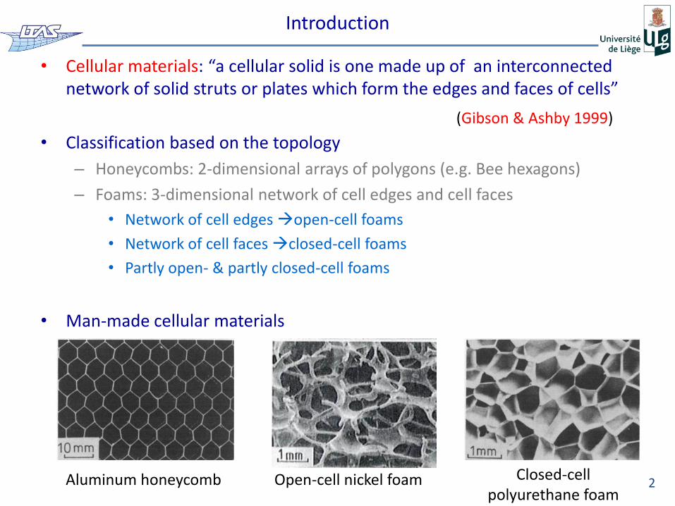
• Cellular materials: “a cellular solid is one made up of an interconnected network of solid struts or plates which form the edges and faces of cells”
• Classification based on the topology
– Honeycombs: 2-dimensional arrays of polygons (e.g. Bee hexagons)
– Foams: 3-dimensional network of cell edges and cell faces
• Network of cell edges open-cell foams
• Network of cell faces closed-cell foams
• Partly open- & partly closed-cell foams
• Man-made cellular materials
2
(Gibson & Ashby 1999)
Aluminum honeycomb Closed-cell polyurethane foam
Open-cell nickel foam
Introduction
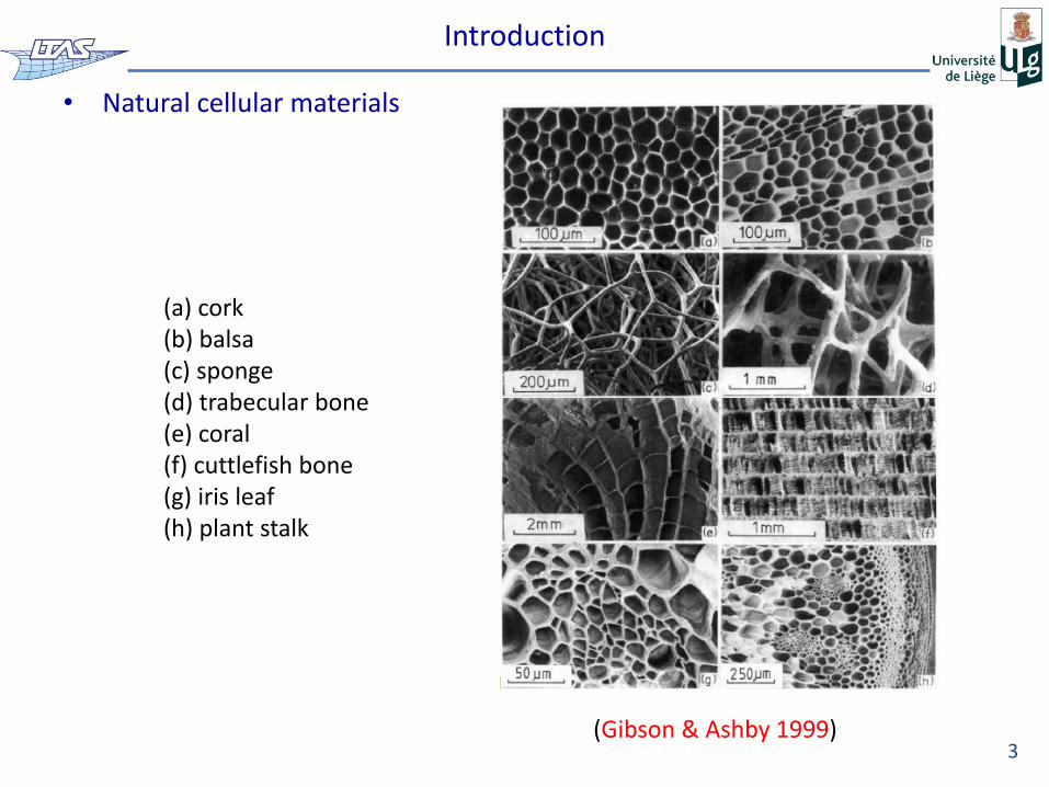
• Natural cellular materials
3 (Gibson & Ashby 1999)
(a) cork (b) balsa (c) sponge (d) trabecular bone (e) coral (f) cuttlefish bone (g) iris leaf (h) plant stalk
Introduction
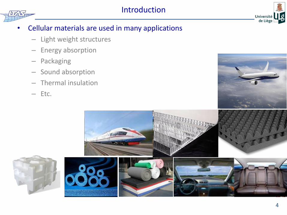
• Cellular materials are used in many applications
– Light weight structures
– Energy absorption
– Packaging
– Sound absorption
– Thermal insulation
– Etc.
4
Introduction
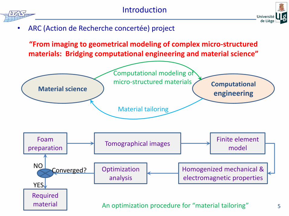
• ARC (Action de Recherche concertée) project
5
“From imaging to geometrical modeling of complex micro-structured materials: Bridging computational engineering and material science”
Foam preparation
Tomographical images
Optimization analysis
Homogenized mechanical & electromagnetic properties
Finite element model
Converged? NO
YES
Required material An optimization procedure for “material tailoring”
Computational
engineering Material science
Computational modeling of micro-structured materials
Material tailoring
Introduction
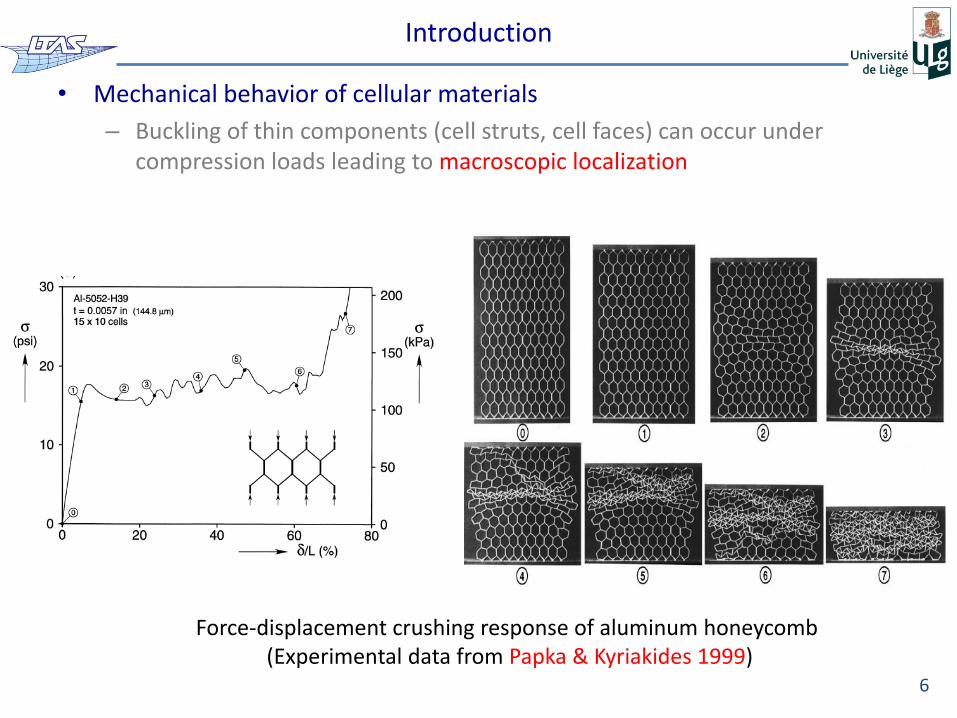
• Mechanical behavior of cellular materials
– Buckling of thin components (cell struts, cell faces) can occur under compression loads leading to macroscopic localization
6
Force-displacement crushing response of aluminum honeycomb (Experimental data from Papka & Kyriakides 1999)
Introduction
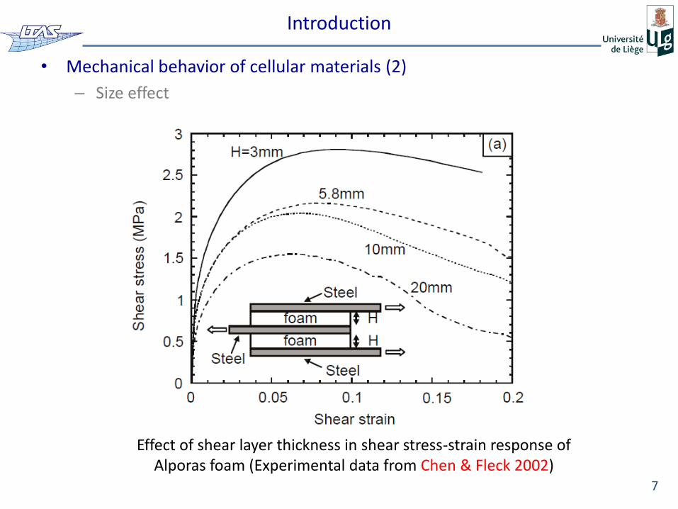
• Mechanical behavior of cellular materials (2)
– Size effect
7
Effect of shear layer thickness in shear stress-strain response of Alporas foam (Experimental data from Chen & Fleck 2002)
Introduction
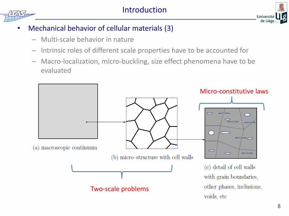
• Mechanical behavior of cellular materials (3)
– Multi-scale behavior in nature
– Intrinsic roles of different scale properties have to be accounted for
– Macro-localization, micro-buckling, size effect phenomena have to be evaluated
8
Two-scale problems
Micro-constitutive laws
Introduction
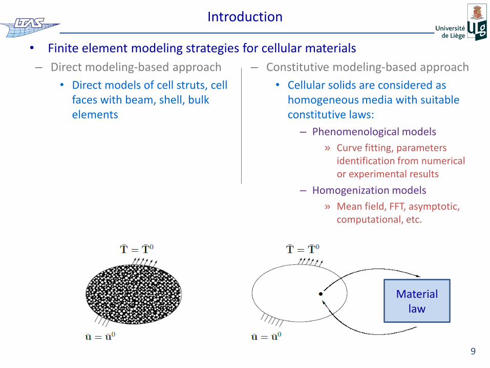
• Finite element modeling strategies for cellular materials
9
– Direct modeling-based approach
• Direct models of cell struts, cell faces with beam, shell, bulk elements
– Constitutive modeling-based approach
• Cellular solids are considered as homogeneous media with suitable constitutive laws:
– Phenomenological models
» Curve fitting, parameters identification from numerical or experimental results
– Homogenization models
» Mean field, FFT, asymptotic, computational, etc.
Material law
Introduction
• Finite element modeling strategies for cellular materials (2)
– Direct modeling-based approach
• Advantages:
– Capture directly localization due to micro-buckling & size effects
• Drawbacks
– Enormous number of DOFs
– Difficult to construct the FE model due to geometry complexities
– Suitable for small problems with limited dimensions
10
Introduction
• Finite element modeling strategies for cellular materials (3)
– Constitutive modeling-based approach
• Advantages
– Suitable for large problems
– Micro-buckling, macro-localization & size effects can be captured with suitable constitutive models (e.g. computational homogenization)
• Drawbacks
– Phenomenological models
» Details of the micro-structure during macro-loading cannot be observed
» Material models and their parameters are difficult to be identified
– Homogenization models
» Occurrence of micro-buckling phenomena is still limited in the mean -field, FFT, asymptotic homogenization frameworks
11
Introduction
• Computational homogenization
– This method is probably the most accurate method to directly account for complex micro-structural behaviors
– This method can model:
• Micro-buckling of cell walls (e.g. Okumura et al. 2004, Takahashi et al. 2010)
• Localization problems (e.g. Kouznetsova et al. 2004, Massart et al. 2007,
Nguyen et al. 2011, Coenen et al. 2012)
• Size effects (e.g. Kouznetsova et al. 2004, Ebinger et al. (2005))
12
Introduction
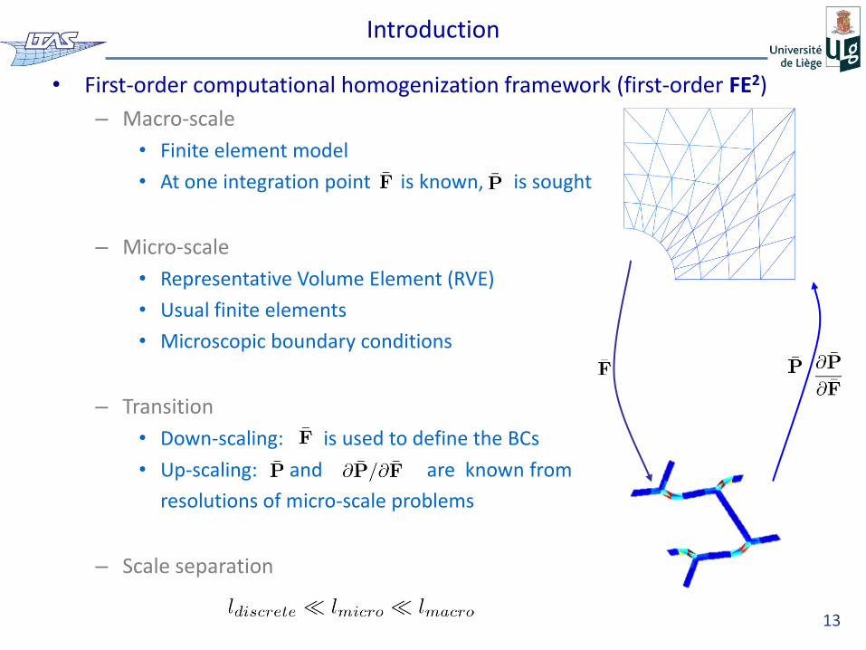
• First-order computational homogenization framework (first-order FE2)
– Macro-scale
• Finite element model
• At one integration point is known, is sought
– Micro-scale
• Representative Volume Element (RVE)
• Usual finite elements
• Microscopic boundary conditions
– Transition
• Down-scaling: is used to define the BCs
• Up-scaling: and are known from
resolutions of micro-scale problems
– Scale separation
13
Introduction
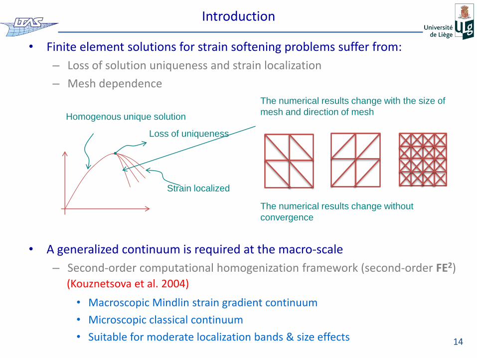
• Finite element solutions for strain softening problems suffer from:
– Loss of solution uniqueness and strain localization
– Mesh dependence
• A generalized continuum is required at the macro-scale
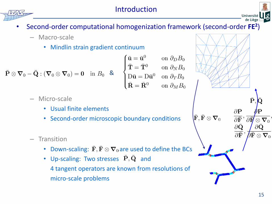
– Second-order computational homogenization framework (second-order FE2)
• Macroscopic Mindlin strain gradient continuum
• Microscopic classical continuum
• Suitable for moderate localization bands & size effects
14
(Kouznetsova et al. 2004)
The numerical results change with the size of
mesh and direction of mesh Homogenous unique solution
Loss of uniqueness
Strain localized
The numerical results change without
convergence
Introduction
• Second-order computational homogenization framework (second-order FE2)
– Macro-scale
• Mindlin strain gradient continuum
– Micro-scale
• Usual finite elements
• Second-order microscopic boundary conditions
– Transition
• Down-scaling: are used to define the BCs
• Up-scaling: Two stresses and
4 tangent operators are known from resolutions of
micro-scale problems
15
&
Introduction
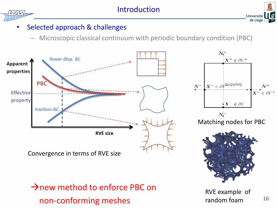
• Selected approach & challenges
– Microscopic classical continuum with periodic boundary condition (PBC)
new method to enforce PBC on
non-conforming meshes 16 RVE example of random foam
Matching nodes for PBC
Convergence in terms of RVE size
Introduction
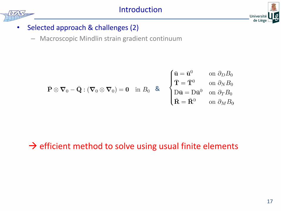
• Selected approach & challenges (2)
– Macroscopic Mindlin strain gradient continuum
17
&
efficient method to solve using usual finite elements
Introduction
• Selected approach & challenges (3)
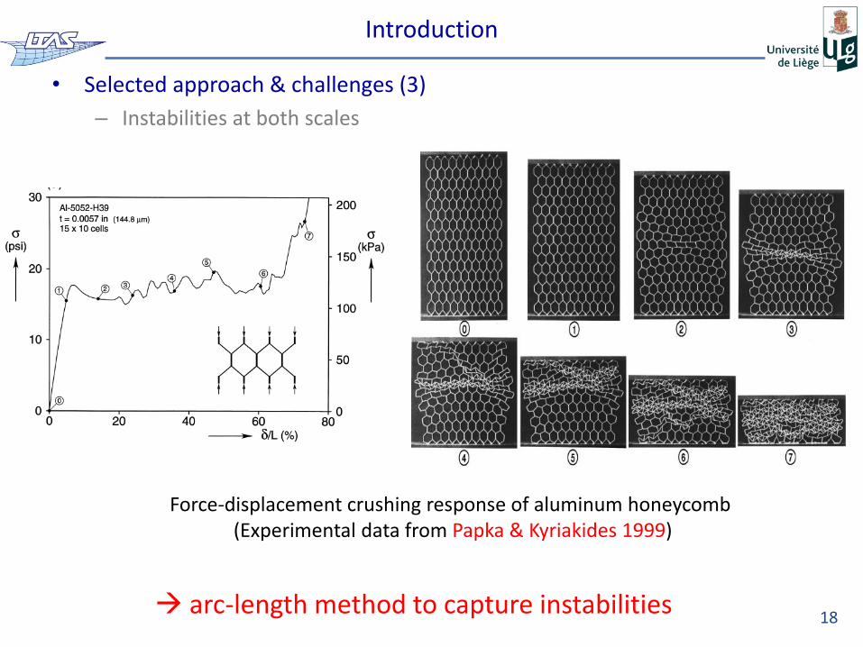
– Instabilities at both scales
18
Force-displacement crushing response of aluminum honeycomb (Experimental data from Papka & Kyriakides 1999)
arc-length method to capture instabilities
Topics
• PBC enforcement based on the polynomial interpolation method
• Second-order multi-scale computational homogenization scheme based on the Discontinuous Galerkin method (called second-order DG-based FE2 scheme)
– DG method is used to solved the macroscopic Mindlin strain gradient
– Usual FE
– Parallel computation
• Use of this second-order DG-based FE2 scheme to capture instabilities in cellular materials
– Arc-length path following method is adopted at both scales because of the presence of the macroscopic localization and micro-buckling
– Parallel computation
19
(Nguyen, Geuzaine, Béchet & Noels CMS 2012)
(Nguyen, Becker & Noels CMAME 2013)
(Nguyen & Noels IJSS 2014)
Topics
• PBC enforcement based on the polynomial interpolation method
• Second-order multi-scale computational homogenization scheme based on the Discontinuous Galerkin method (called second-order DG-based FE2 scheme)
– DG method is used to solved the macroscopic Mindlin strain gradient
– Usual FE
– Parallel computation
• Use of this second DG-based FE2 scheme to capture instabilities in cellular materials
– Arc-length path following method is adopted at both scales because of the presence of the macroscopic localization and micro-buckling
– Parallel computation
20
(Nguyen, Geuzaine, Béchet & Noels CMS 2012)
(Nguyen, Becker & Noels CMAME 2013)
(Nguyen & Noels IJSS 2014)
Polynomial interpolation method
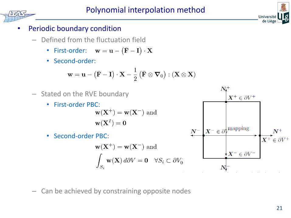
• Periodic boundary condition
– Defined from the fluctuation field
• First-order:
• Second-order:
– Stated on the RVE boundary
• First-order PBC:
• Second-order PBC:
– Can be achieved by constraining opposite nodes
21
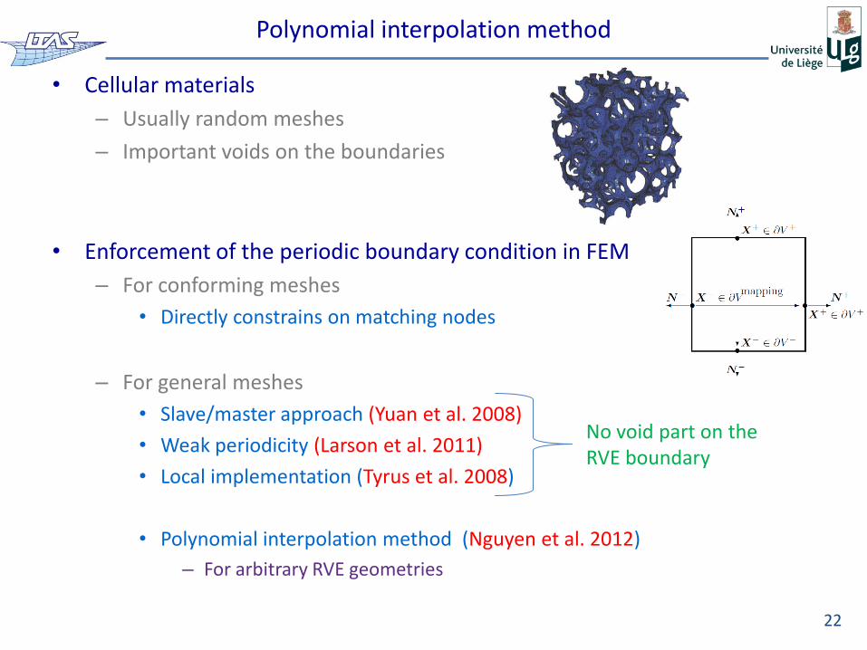
Polynomial interpolation method
• Cellular materials
– Usually random meshes
– Important voids on the boundaries
• Enforcement of the periodic boundary condition in FEM
– For conforming meshes
• Directly constrains on matching nodes
– For general meshes
• Slave/master approach (Yuan et al. 2008)
• Weak periodicity (Larson et al. 2011)
• Local implementation (Tyrus et al. 2008)
• Polynomial interpolation method (Nguyen et al. 2012)
– For arbitrary RVE geometries
22
No void part on the RVE boundary
Polynomial interpolation method
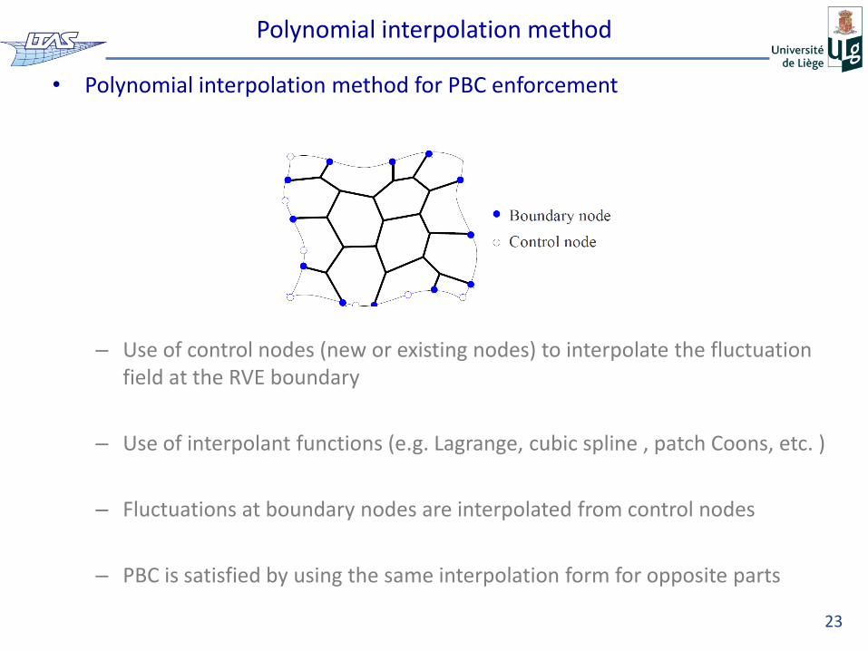
• Polynomial interpolation method for PBC enforcement
– Use of control nodes (new or existing nodes) to interpolate the fluctuation field at the RVE boundary
– Use of interpolant functions (e.g. Lagrange, cubic spline , patch Coons, etc. )
– Fluctuations at boundary nodes are interpolated from control nodes
– PBC is satisfied by using the same interpolation form for opposite parts
23
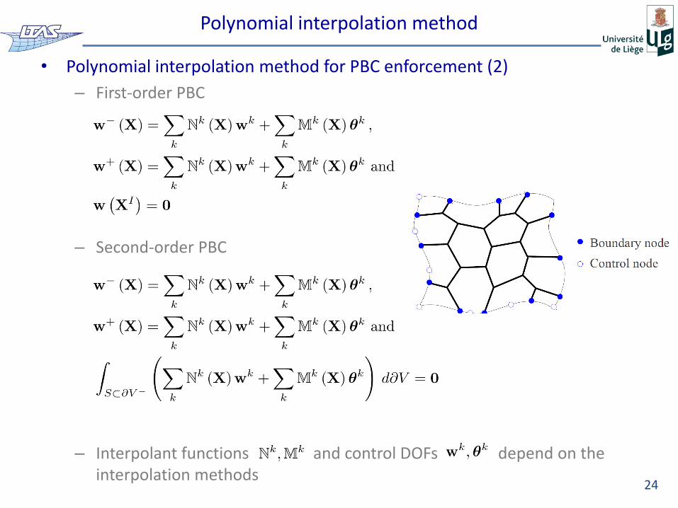
Polynomial interpolation method
• Polynomial interpolation method for PBC enforcement (2)
– First-order PBC
– Second-order PBC
– Interpolant functions and control DOFs depend on the interpolation methods
24
Polynomial interpolation method
• Polynomial interpolation method for PBC enforcement (3)
– Results in new constraints in terms of displacements of both boundary and control nodes
• First order:
• Second-order:
– These linear constraints can be enforced by
• Constraints elimination
• Lagrange multipliers
– Suitable for
• Arbitrary meshes
• Important void parts on the RVE boundaries
• Arbitrary interpolation forms
25
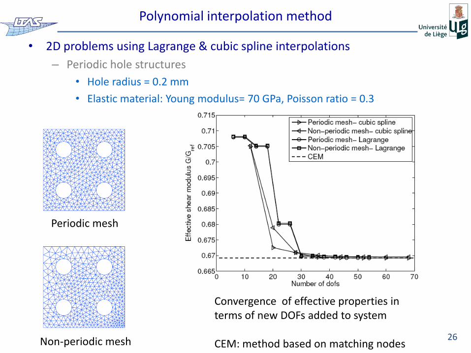
Polynomial interpolation method
• 2D problems using Lagrange & cubic spline interpolations
– Periodic hole structures
• Hole radius = 0.2 mm
• Elastic material: Young modulus= 70 GPa, Poisson ratio = 0.3
26
Periodic mesh
Non-periodic mesh CEM: method based on matching nodes
Convergence of effective properties in terms of new DOFs added to system
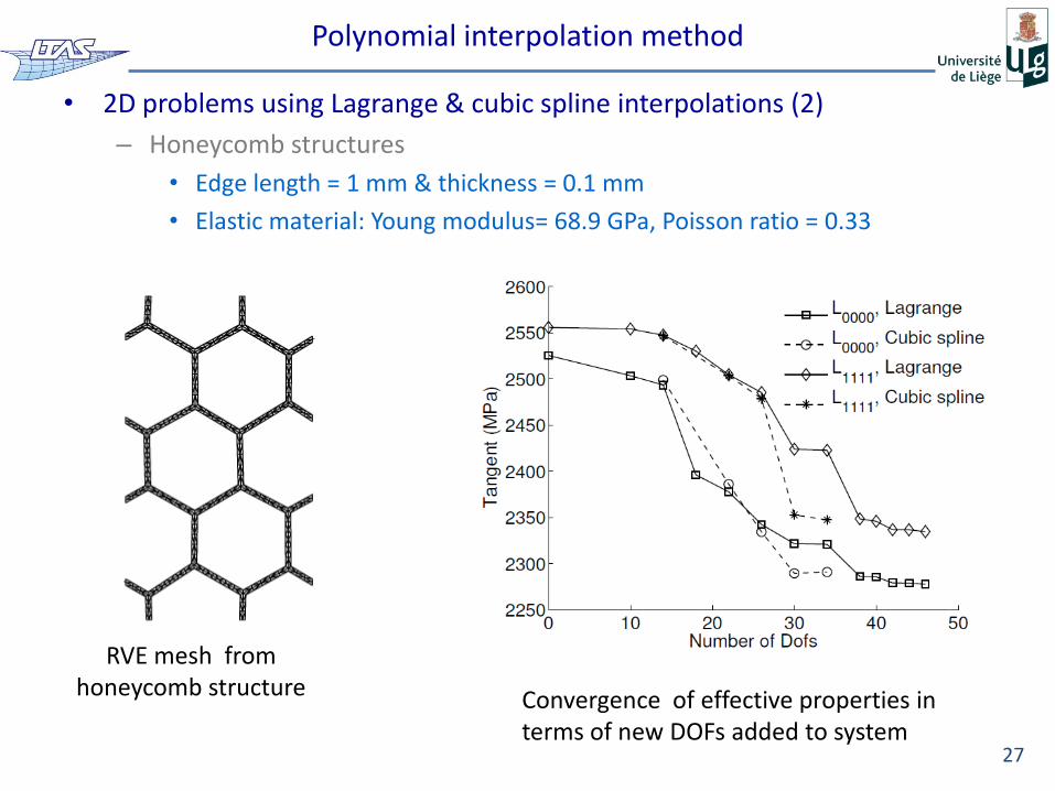
Polynomial interpolation method
• 2D problems using Lagrange & cubic spline interpolations (2)
– Honeycomb structures
• Edge length = 1 mm & thickness = 0.1 mm
• Elastic material: Young modulus= 68.9 GPa, Poisson ratio = 0.33
27
Convergence of effective properties in terms of new DOFs added to system
RVE mesh from honeycomb structure
Polynomial interpolation method
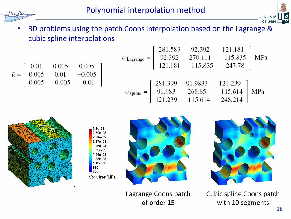
• 3D problems using the patch Coons interpolation based on the Lagrange & cubic spline interpolations
28
Cubic spline Coons patch with 10 segments
Lagrange Coons patch of order 15
Polynomial interpolation method
• Conclusions
– A new method to enforce the PBC is presented
• By using an interpolation formulation
• For arbitrary meshes
• For both 2-dimensional and 3-dimensional problems
– This method provides a better estimation compared to the linear displacement BC which is usually used for non-conforming meshes
– The key advantage of this method is the elimination of the need of matching nodes
29
Topics
• PBC enforcement based on the polynomial interpolation method
• Second-order multi-scale computational homogenization scheme based on the Discontinuous Galerkin method (called second-order DG-based FE2 scheme)
– DG method is used to solved the macroscopic Mindlin strain gradient
– Usual FE
– Parallel computation
• Use of this second DG-based FE2 scheme to capture instabilities in cellular materials
– Arc-length path following method is adopted at both scales because of the presence of the macroscopic localization and micro-buckling
– Parallel computation
30
(Nguyen, Geuzaine, Béchet & Noels CMS 2012)
(Nguyen, Becker & Noels CMAME 2013)
(Nguyen & Noels IJSS 2014)
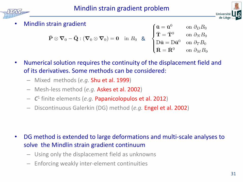
Mindlin strain gradient problem
• Mindlin strain gradient
• Numerical solution requires the continuity of the displacement field and of its derivatives. Some methods can be considered:
– Mixed methods (e.g. Shu et al. 1999)
– Mesh-less method (e.g. Askes et al. 2002)
– C1 finite elements (e.g. Papanicolopulos et al. 2012)
– Discontinuous Galerkin (DG) method (e.g. Engel et al. 2002)
• DG method is extended to large deformations and multi-scale analyses to solve the Mindlin strain gradient continuum
– Using only the displacement field as unknowns
– Enforcing weakly inter-element continuities
31
&
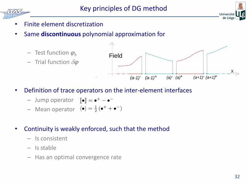
Key principles of DG method
• Finite element discretization
• Same discontinuous polynomial approximation for
– Test function h
– Trial function d
• Definition of trace operators on the inter-element interfaces
– Jump operator
– Mean operator
• Continuity is weakly enforced, such that the method
– Is consistent
– Is stable
– Has an optimal convergence rate
32
(a-1) - (a-1) + (a) - (a) + (a+1) - X
(a+1) +
Field
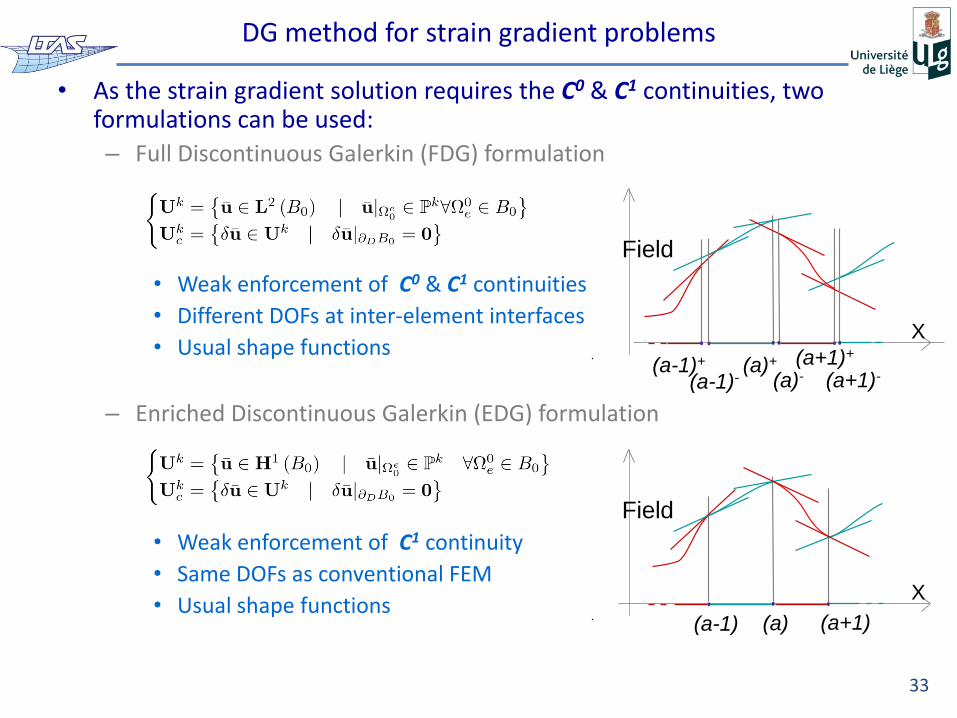
DG method for strain gradient problems
• As the strain gradient solution requires the C0 & C1 continuities, two formulations can be used:
– Full Discontinuous Galerkin (FDG) formulation
• Weak enforcement of C0 & C1 continuities
• Different DOFs at inter-element interfaces
• Usual shape functions
– Enriched Discontinuous Galerkin (EDG) formulation
• Weak enforcement of C1 continuity
• Same DOFs as conventional FEM
• Usual shape functions
33
(a-1) (a)
X
(a+1)
Field
(a-1)+ (a)+
X
(a+1)+
Field
(a-1)- (a)- (a+1)-
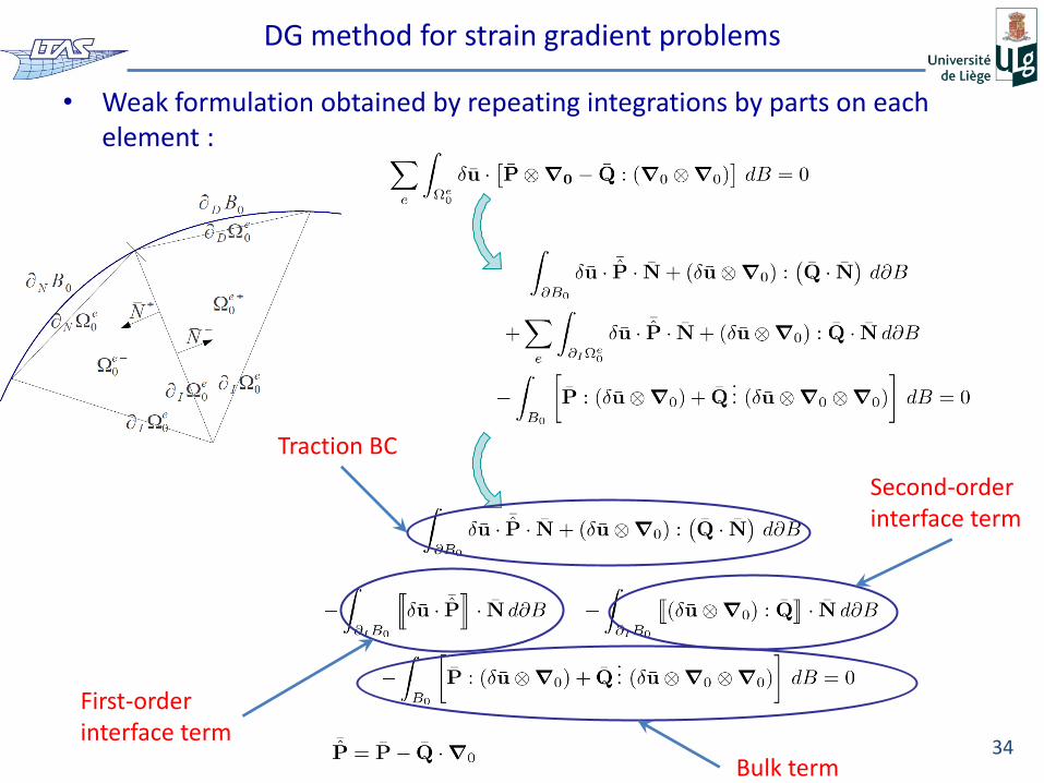
DG method for strain gradient problems
• Weak formulation obtained by repeating integrations by parts on each element :
34
First-order interface term
Second-order interface term
Traction BC
Bulk term
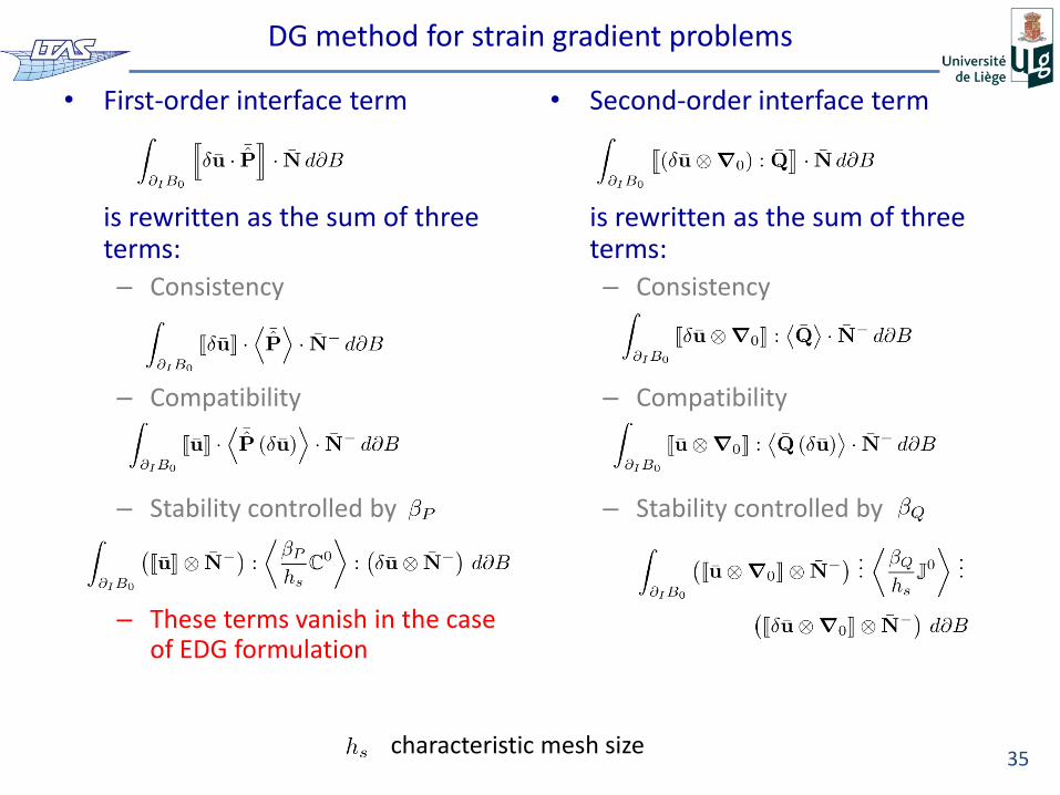
DG method for strain gradient problems
• First-order interface term
is rewritten as the sum of three terms:
– Consistency
– Compatibility
– Stability controlled by
– These terms vanish in the case of EDG formulation
• Second-order interface term
is rewritten as the sum of three terms:
– Consistency
– Compatibility
– Stability controlled by
35 characteristic mesh size
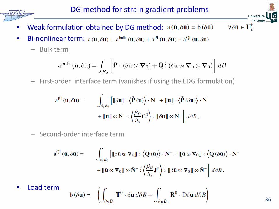
DG method for strain gradient problems
• Weak formulation obtained by DG method:
• Bi-nonlinear term:
– Bulk term
– First-order interface term (vanishes if using the EDG formulation)
– Second-order interface term
• Load term
36
DG method for strain gradient problems
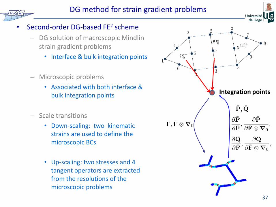
• Second-order DG-based FE2 scheme
– DG solution of macroscopic Mindlin strain gradient problems
• Interface & bulk integration points
– Microscopic problems
• Associated with both interface & bulk integration points
– Scale transitions
• Down-scaling: two kinematic strains are used to define the microscopic BCs
• Up-scaling: two stresses and 4 tangent operators are extracted from the resolutions of the microscopic problems
37
Integration points
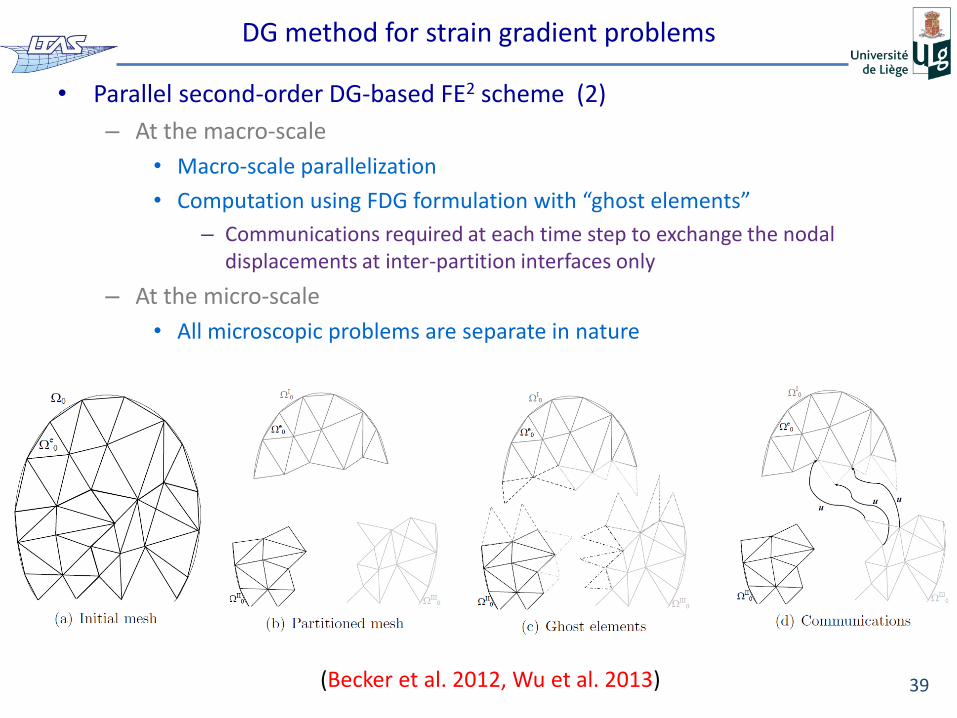
DG method for strain gradient problems
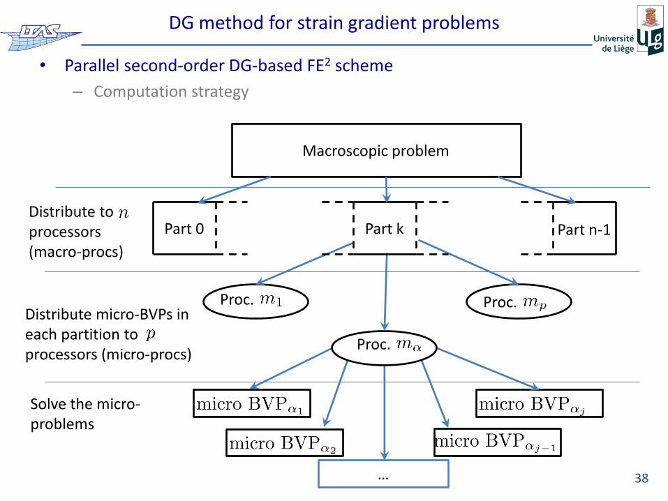
• Parallel second-order DG-based FE2 scheme
– Computation strategy
Macroscopic problem
Solve the micro-problems
…
Distribute micro-BVPs in each partition to processors (micro-procs)
Proc. Proc.
Proc.
Part 0 Part n-1 Part k Distribute to processors (macro-procs)
38
DG method for strain gradient problems
• Parallel second-order DG-based FE2 scheme (2)
– At the macro-scale
• Macro-scale parallelization
• Computation using FDG formulation with “ghost elements”
– Communications required at each time step to exchange the nodal displacements at inter-partition interfaces only
– At the micro-scale
• All microscopic problems are separate in nature
39 (Becker et al. 2012, Wu et al. 2013)
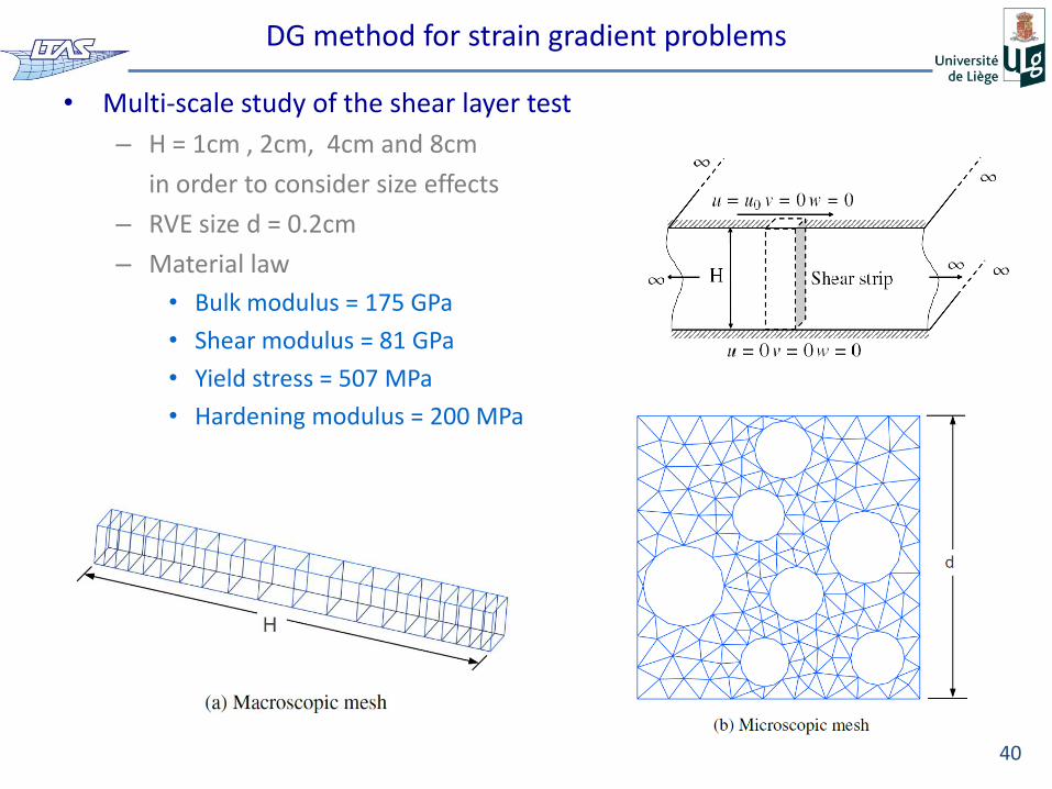
DG method for strain gradient problems
• Multi-scale study of the shear layer test
– H = 1cm , 2cm, 4cm and 8cm
in order to consider size effects
– RVE size d = 0.2cm
– Material law
• Bulk modulus = 175 GPa
• Shear modulus = 81 GPa
• Yield stress = 507 MPa
• Hardening modulus = 200 MPa
40
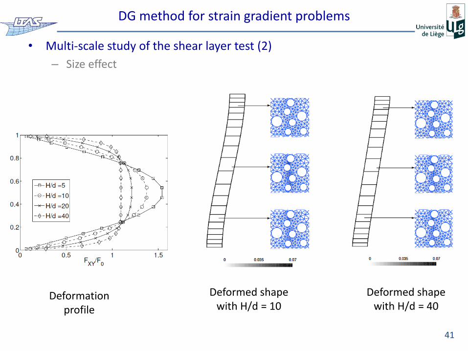
DG method for strain gradient problems
• Multi-scale study of the shear layer test (2)
– Size effect
41
Deformed shape with H/d = 10
Deformed shape with H/d = 40
Deformation profile
DG method for strain gradient problems
• Conclusions
– The Mindlin strain gradient problems are solved using the discontinuous Galerkin formulations with conventional finite elements
– The resulting one-field formulation can easily be implemented in existing software
– This formulation is used for second-order multi-scale computational homogenizations
– The micro and macro-scale problems consider finite strains
– Size effects in heterogeneous elasto–plastic materials can be studied
42
Topics
• PBC enforcement based on the polynomial interpolation method
• Second-order multi-scale computational homogenization scheme based on the Discontinuous Galerkin method (called second-order DG-based FE2 scheme)
– DG method is used to solved the macroscopic Mindlin strain gradient
– Usual FE
– Parallel computation
• Use of this second-order DG-based FE2 scheme to capture instabilities in cellular materials
– Arc-length path following method is adopted at both scales because of the presence of the macroscopic localization and micro-buckling
– Parallel computation
43
(Nguyen, Geuzaine, Béchet & Noels CMS 2012)
(Nguyen, Becker & Noels CMAME 2013)
(Nguyen & Noels IJSS 2014)
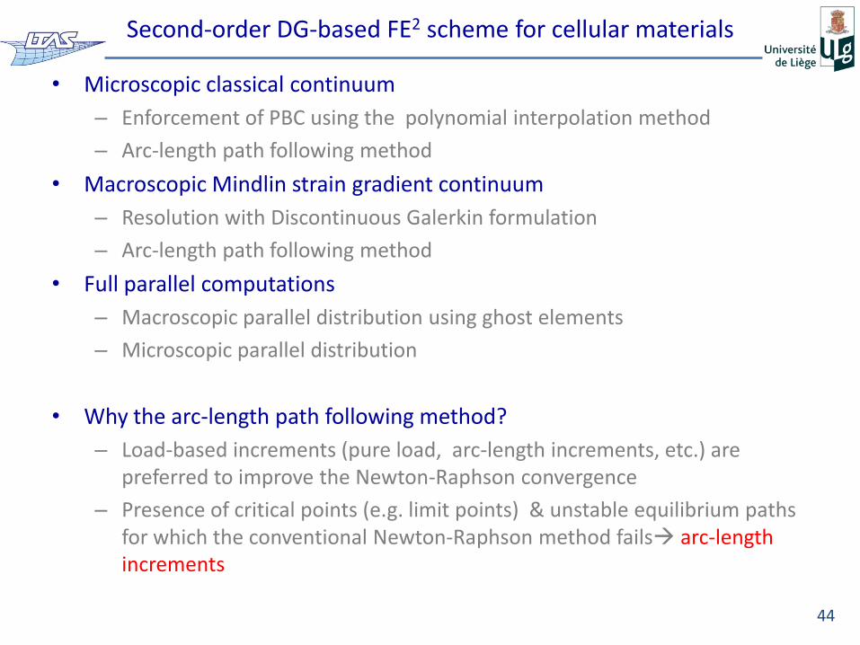
Second-order DG-based FE2 scheme for cellular materials
• Microscopic classical continuum
– Enforcement of PBC using the polynomial interpolation method
– Arc-length path following method
• Macroscopic Mindlin strain gradient continuum
– Resolution with Discontinuous Galerkin formulation
– Arc-length path following method
• Full parallel computations
– Macroscopic parallel distribution using ghost elements
– Microscopic parallel distribution
• Why the arc-length path following method?
– Load-based increments (pure load, arc-length increments, etc.) are preferred to improve the Newton-Raphson convergence
– Presence of critical points (e.g. limit points) & unstable equilibrium paths for which the conventional Newton-Raphson method fails arc-length increments
44
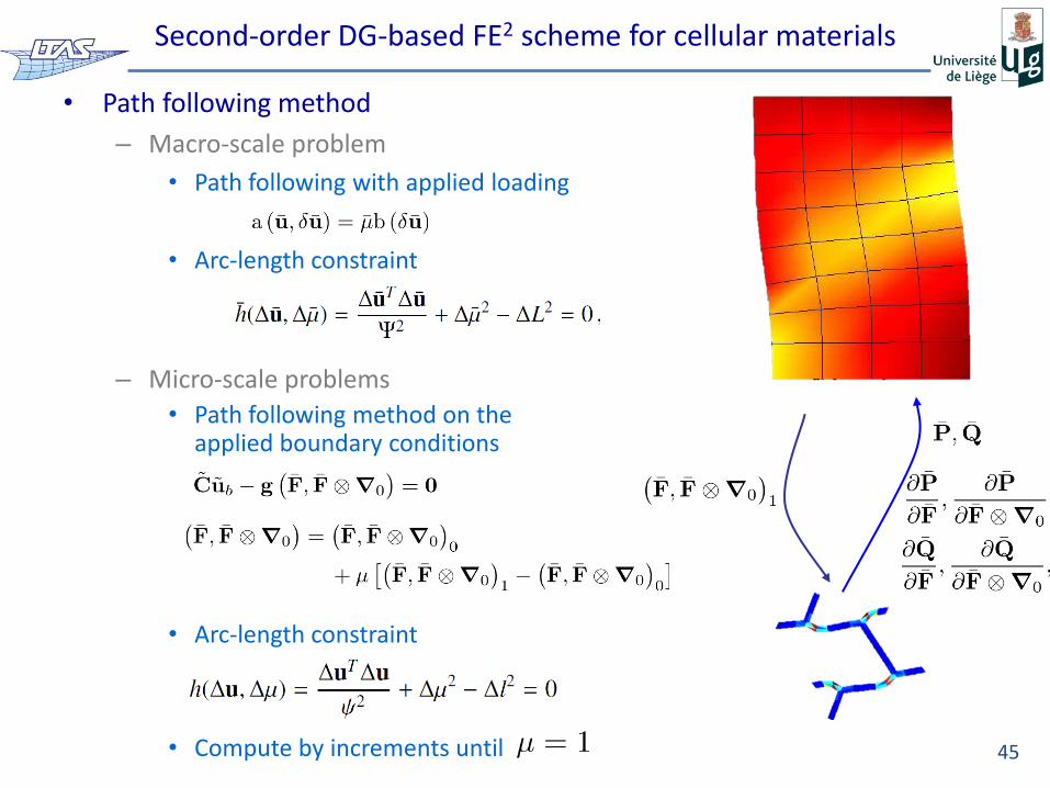
Second-order DG-based FE2 scheme for cellular materials
• Path following method
– Macro-scale problem
• Path following with applied loading
• Arc-length constraint
– Micro-scale problems
• Path following method on the applied boundary conditions
• Arc-length constraint
• Compute by increments until
45
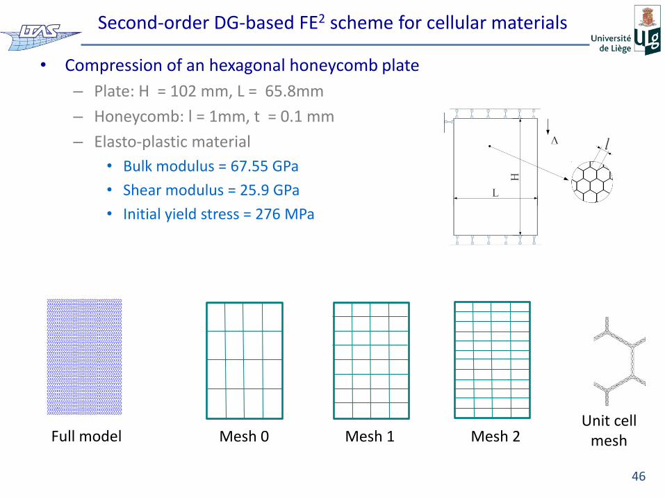
Second-order DG-based FE2 scheme for cellular materials
• Compression of an hexagonal honeycomb plate
– Plate: H = 102 mm, L = 65.8mm
– Honeycomb: l = 1mm, t = 0.1 mm
– Elasto-plastic material
• Bulk modulus = 67.55 GPa
• Shear modulus = 25.9 GPa
• Initial yield stress = 276 MPa
46
Unit cell mesh Full model Mesh 0 Mesh 1 Mesh 2
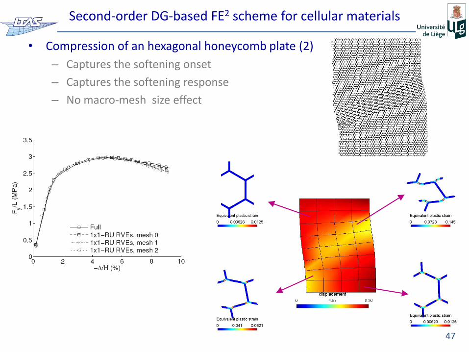
Second-order DG-based FE2 scheme for cellular materials
• Compression of an hexagonal honeycomb plate (2)
– Captures the softening onset
– Captures the softening response
– No macro-mesh size effect
47
Second-order DG-based FE2 scheme for cellular materials
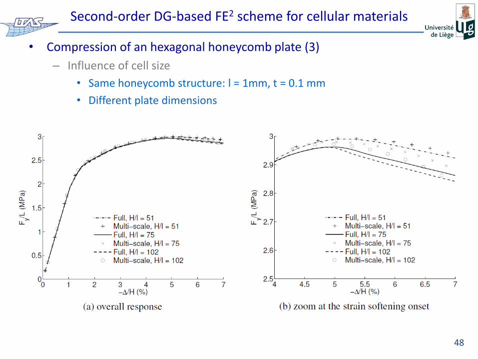
• Compression of an hexagonal honeycomb plate (3)
– Influence of cell size
• Same honeycomb structure: l = 1mm, t = 0.1 mm
• Different plate dimensions
48
Second-order DG-based FE2 scheme for cellular materials
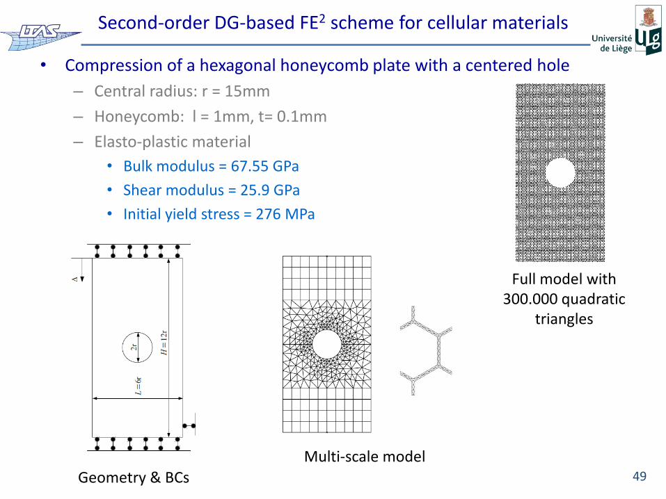
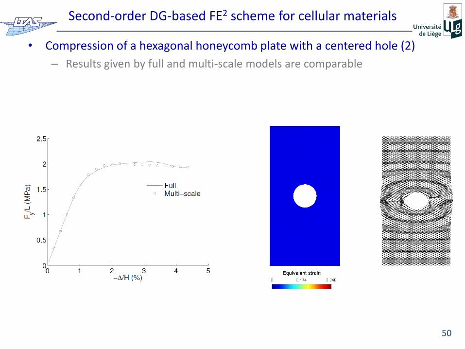
• Compression of a hexagonal honeycomb plate with a centered hole
– Central radius: r = 15mm
– Honeycomb: l = 1mm, t= 0.1mm
– Elasto-plastic material
• Bulk modulus = 67.55 GPa
• Shear modulus = 25.9 GPa
• Initial yield stress = 276 MPa
49
Multi-scale model
Geometry & BCs
Full model with 300.000 quadratic
triangles
Second-order DG-based FE2 scheme for cellular materials
• Compression of a hexagonal honeycomb plate with a centered hole (2)
– Results given by full and multi-scale models are comparable
50
Second-order DG-based FE2 scheme for cellular materials
• A second-order DG-based FE2 scheme was developed with the following novelties:
– The periodic boundary condition is enforced using the polynomial interpolation method without the need of conforming meshes
– The macroscopic Mindlin strain gradient problem is solved using the Discontinuous Galerkin method with conventional finite elements
– The arc-length path following method is applied at both scales to capture their instabilities
51
Current works
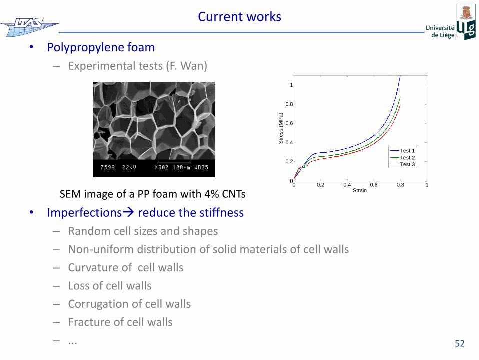
• Polypropylene foam
– Experimental tests (F. Wan)
• Imperfections reduce the stiffness
– Random cell sizes and shapes
– Non-uniform distribution of solid materials of cell walls
– Curvature of cell walls
– Loss of cell walls
– Corrugation of cell walls
– Fracture of cell walls
– ...
52
0 0.2 0.4 0.6 0.8 10
0.2
0.4
0.6
0.8
1
Strain
Str
ess (
MP
a)
Test 1
Test 2
Test 3
SEM image of a PP foam with 4% CNTs
Current works
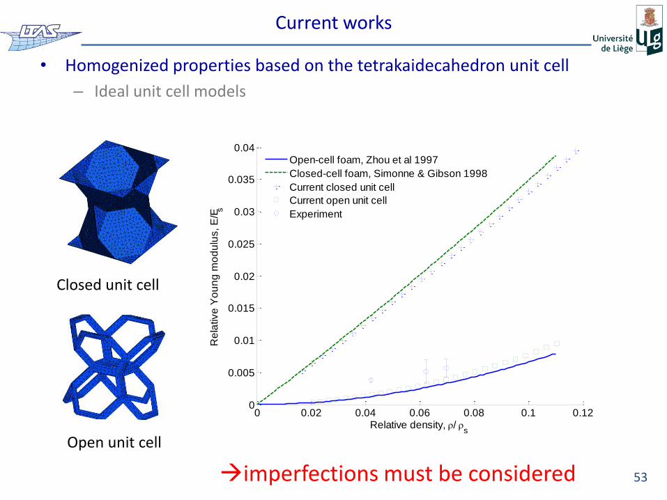
• Homogenized properties based on the tetrakaidecahedron unit cell
– Ideal unit cell models
53
Closed unit cell
Open unit cell
0 0.02 0.04 0.06 0.08 0.1 0.120
0.005
0.01
0.015
0.02
0.025
0.03
0.035
0.04
Relative density, / s
Re
lative
Yo
un
g m
od
ulu
s, E
/Es
Open-cell foam, Zhou et al 1997
Closed-cell foam, Simonne & Gibson 1998
Current closed unit cell
Current open unit cell
Experiment
imperfections must be considered
Current works
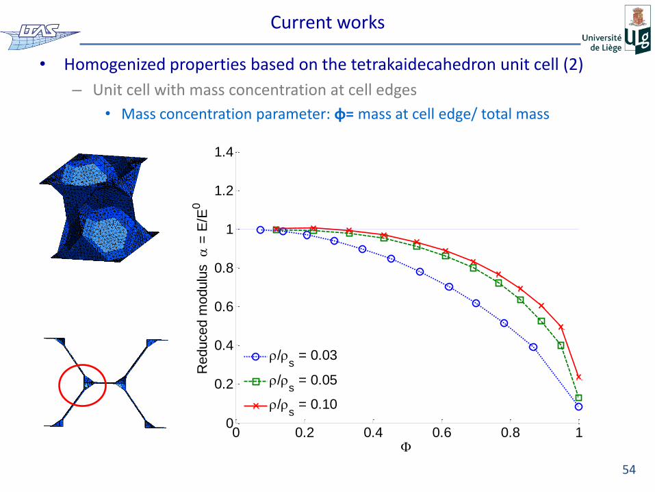
• Homogenized properties based on the tetrakaidecahedron unit cell (2)
– Unit cell with mass concentration at cell edges
• Mass concentration parameter: φ= mass at cell edge/ total mass
54
0 0.2 0.4 0.6 0.8 10
0.2
0.4
0.6
0.8
1
1.2
1.4
Reduced m
odulu
s
=
E/E
0
/s = 0.03
/s = 0.05
/s = 0.10
Perspectives
• Experimental validation in the context of the ARC project with the RVE meshes coming from tomographical images of the microstructure
• Electromagnetic-mechanical coupling problems since electromagnetic properties are modified during the mechanical loading (as the shape is deformed)
• Discontinuous-continuous schemes for sharper localization problems following the works of Massart et al. 2007, Nguyen et al. 2011 or Coenen et al. 2012
• Material tailoring with required properties by computational homogenization schemes
• …
55

56
Thank you for your attention!
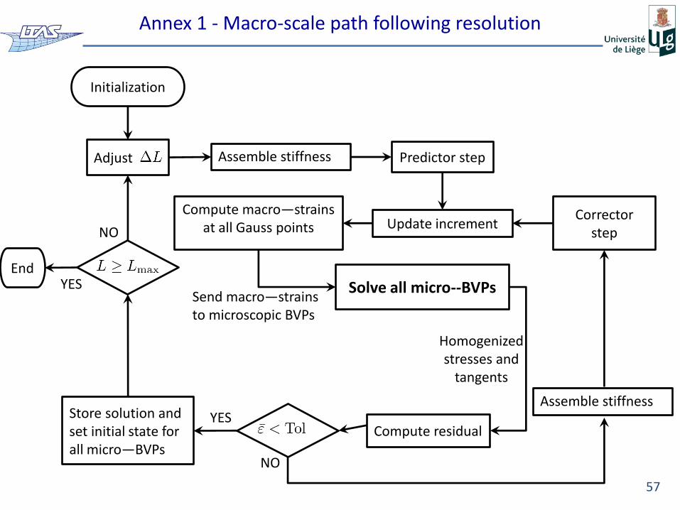
Annex 1 - Macro-scale path following resolution
Corrector step
Update increment
Solve all micro--BVPs End
Predictor step
YES
YES
NO
NO
Compute macro—strains at all Gauss points
Assemble stiffness
Store solution and set initial state for all micro—BVPs
Send macro—strains to microscopic BVPs
Homogenized stresses and
tangents
Initialization
Adjust
Compute residual
57
Assemble stiffness
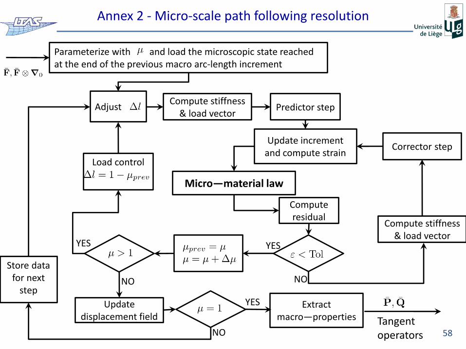
Annex 2 - Micro-scale path following resolution
Corrector step
Predictor step
YES
Adjust
Update increment and compute strain
Parameterize with and load the microscopic state reached at the end of the previous macro arc-length increment
Compute stiffness & load vector
Update displacement field
Load control
Store data for next
step
Compute residual
YES
YES
NO NO
NO
Micro—material law
Extract macro—properties
58 Tangent operators
Compute stiffness & load vector
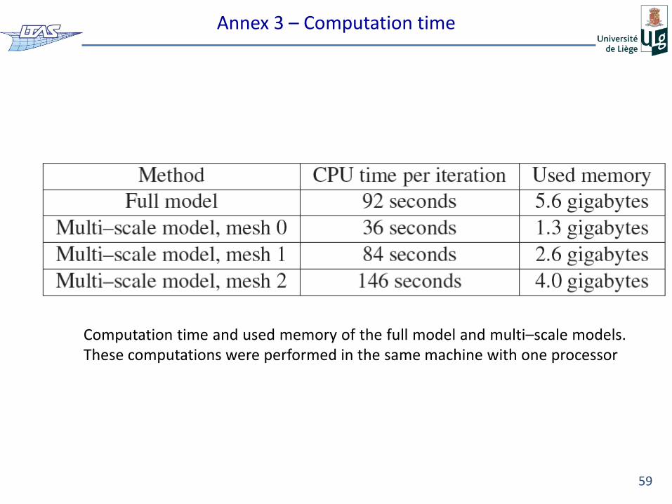
Annex 3 – Computation time
59
Computation time and used memory of the full model and multi–scale models. These computations were performed in the same machine with one processor