Towards Realization of

Computational Homogenization in Practice1

Zheng Yuan and Jacob Fish

Department of Mechanical, Aerospace and Nuclear Engineering Rensselaer Polytechnic Institute

Troy, NY 12180, USA fishj@rpi.edu

Abstract

We present a computational homogenization approach for linear and nonlinear solid

mechanics problems, which is fully compatible with conventional finite element code architecture.

A seamless implementation in ABAQUS is presented including Python script, validation problems

and a web-link where script files, user-defined subroutines and input files can be accessed. For

linear problems, we demonstrate how to utilize ABAQUS existing facilities to develop analysis

attributes required for solving a unit cell problem. For nonlinear problems, a Python script invoked

by a coarse scale stress update procedure is introduced to carry out the scale bridging. The

purpose of this paper is twofold: (i) to motivate practitioners to adopt the computational

homogenization as an integral part of their analysis and design process; and (ii) to encourage

commercial code vendors to seamlessly integrate the architectures proposed in their legacy

codes.

1. Introduction Composite materials evolved from humble beginnings, such as ancient mud bricks

reinforced with straw, 7000-year old bitumen covered reed boats, and American Indian wood and mud structures to premier man-made building blocks in modern-day society. Today, composite materials are used increasingly in high-performance applications that

1 Submitted to IJNME, March 2006

require high specific strength and/or stiffness, low electrical conductivity, transparency to radio emissions, resistance to corrosion, etc. According to the E-Composites research study [1], the aerospace industry alone is estimated to use $4.6 billion worth of composite materials during 2005-2010. During this period, the global end product market for composites is projected to reach $27 billion.

Numerous theories have been developed to predict the behavior of composite materials. Starting from the rule of mixtures dating back to the Renaissance era to various effective medium models of Eshelby [2], Hashin [3], Mori and Tanaka [4], self-consistent approaches of Hill [5] and Christensen [6] among many others to various mathematical homogenization methods pioneered by Bensoussan [ 7 ] and Sanchez-Palencia [ 8 ]. Computational aspects of homogenization have been an active area of research starting with a seminal contribution of Guedes and Kikuchi [9] for linear elasticity problems. Over the past decade major contributions have been made to extending the theory of computational homogenization to nonlinear regime [10, 11, 12, 13] and to improving fidelity and computational efficiency of numerical simulations [14,15,16,17,18,19, 20,21, 22, 23,24].

Today, computational homogenization technologies are rapidly maturing with computational efficiency remaining an outstanding issue. Yet, the adoption of these technologies by industry is at an embryonic stage. Historically, industry adopts a new (computational) technology only after it perceives solid evidence that it can shorten time-to-market cycle of a product or process. Over the past 15 years, computational homogenization technologies have been successfully verified and validated; and while industry have abandoned in-house finite element code development efforts and generally shied away from “academic” codes, commercial finite element software vendors have been slow to providing these capabilities. The main reason is not in lack of maturity as one may expect, but in perceived need for entirely new data structures that cannot be accommodated within conventional finite element code architectures.

There are two critical issues that have to be addressed in order to integrate computational homogenization technologies into conventional finite element code architectures:

1. Analysis attributes: the need to develop and to seamlessly integrate new analysis attributes, such as multiple overall strain loadings, periodic boundary conditions, etc.

2. Scale bridging mechanism: the need to control the fine scale problem from the coarse scale analysis, including proper data transfer and manipulation between the scales.

In this paper, we demonstrate how a two-scale analysis can be seamlessly carried out using ABAQUS for both linear and nonlinear solid mechanics problems. For linear problems, we demonstrate how to utilize ABAQUS existing facilities to develop analysis attributes required for solving a unit cell problem. For nonlinear problems, a Python

script invoked by a coarse scale stress update procedure is introduced to carry out the scale bridging. A web-link is provided for user-defined subroutines, Python script and input files for use with ABAQUS code.

2. Linear computational homogenization Using mathematical homogenization, a linear elastostatics problem with periodic coefficients can be decomposed (see Appendix for details and Remark 2 for nomenclature) into uncoupled fine and coarse scale problems: a. Coarse scale problem

,

( ) :

0

;j

ci

cijmn mn x i

ci i u ij j i t

Find u on such that

L b on

u u on n t on

ε

σ

Ω

+ = Ω

= Γ = Γ

x

(1)

where x and y x /ζ= are coarse and fine scale position vectors, respectively; 0 1ζ< ;

ciu is the coarse scale displacement; ( ),

12n

c cc c m nmn m x

n m

u uux x

ε⎛ ⎞∂ ∂

= = +⎜ ⎟∂ ∂⎝ ⎠ the coarse scale strain;

and ib the average unit cell body force. Summation convention is employed for repeated indices. b. Fine-scale (unit cell) problem

( )( , ) ,

( ) :

0

( ) ( )

( ) 0

lj

imn

ijkl k y mn klmn y

imn imn

vertimn

Find on such that

L I on

on

on

χ

χ

χ χ

χ

Θ

⎡ ⎤+ = Θ⎣ ⎦

= + ∂Θ

= ∂Θ

Y

y

y yy

(2)

where ( ) / 2klmn mk nl nk mlI δ δ δ δ= + ; Θ the domain of the unit cell; vert∂Θ the vertices of the

unit cell; and ijmnL the homogenized constitutive tensor components given as

1 mn

ijmn ijL dσΘ

= ΘΘ ∫ (3)

where ( )mnijσ y are stress influence functions (i.e., stress induced by an overall unit strain

cmnε ) defined as

( )( ), l

mnij ijkl klmnk y mnL Iσ χ= + (4)

Finite element discretization of the coarse and fine scale fields, ( )c c ci iA Au N d= x ,

( )f fmnk kA mnAN dχ = y , respectively, gives the two-scale matrix equations:

a. Discrete coarse-scale problem

( )

t

AB A

c c c c cijA ijkl klB B iA i iA i

K F

c cB B u

B L B d d N b d N t d

d d x on

Ω Ω ΓΩ⋅ = Ω+ Ω

= Γ

∫ ∫ ∫ (5)

b. Discrete fine-scale problem

; 0AB mnA

f f f fijA ijkl klB mnB ijA ijmn

K F

f f vertmnB mnB

B L B d d B L d on

d periodic on d on

Θ ΘΘ⋅ = − Θ Θ

∂Θ = ∂Θ

∫ ∫ (6)

where the subscript A denotes degrees-of-freedom; superscripts c and f denote coarse and fine scale fields; ( ), j

f fijA i x A

B N= and ( ), j

c cijA i x A

B N= are symmetric gradients of the corresponding shape functions.

In the following, we focus on implementation of the two-scale analysis in a commercial package of choice. Examples are given for implementation in ABAQUS. The two-scale linear elasticity analysis consists of the following four steps:

1. Solve a unit cell problem with multiple right hand side (RHS) vectors (Eq. (6)) and compute the stress influence functions;

2. Evaluate the overall constitutive tensor components ijmnL by Eq. (3);

3. Solve the coarse-scale problem; and

4. Postprocess stresses in critical (or all) unit cells

We start with Step 1, solution of a unit cell problem subjected to multiple RHS vectors (six in 3D due to symmetry of indices mn). In the matrix implementation, ijmnL is a 6 6× matrix where ij represents six rows and mn six columns. Each column in ijmnL can

be extracted by multiplying ijmnL with a unit overall strain, 1cmnε = . For implementation

in a commercial package, it is convenient to select cmnε in the form of a unit thermal strain

as

κcmn mn Tε = ⋅Δ (7)

where κmn and 1TΔ = are appropriately chosen thermal expansion coefficients and a unit temperature change. Multiple RHS vectors in Eq. (6) can be imposed by changing the thermal expansion coefficient for each loading case as shown in Table I. One way to accomplish it, is by submitting six separate jobs with different values of κmn .

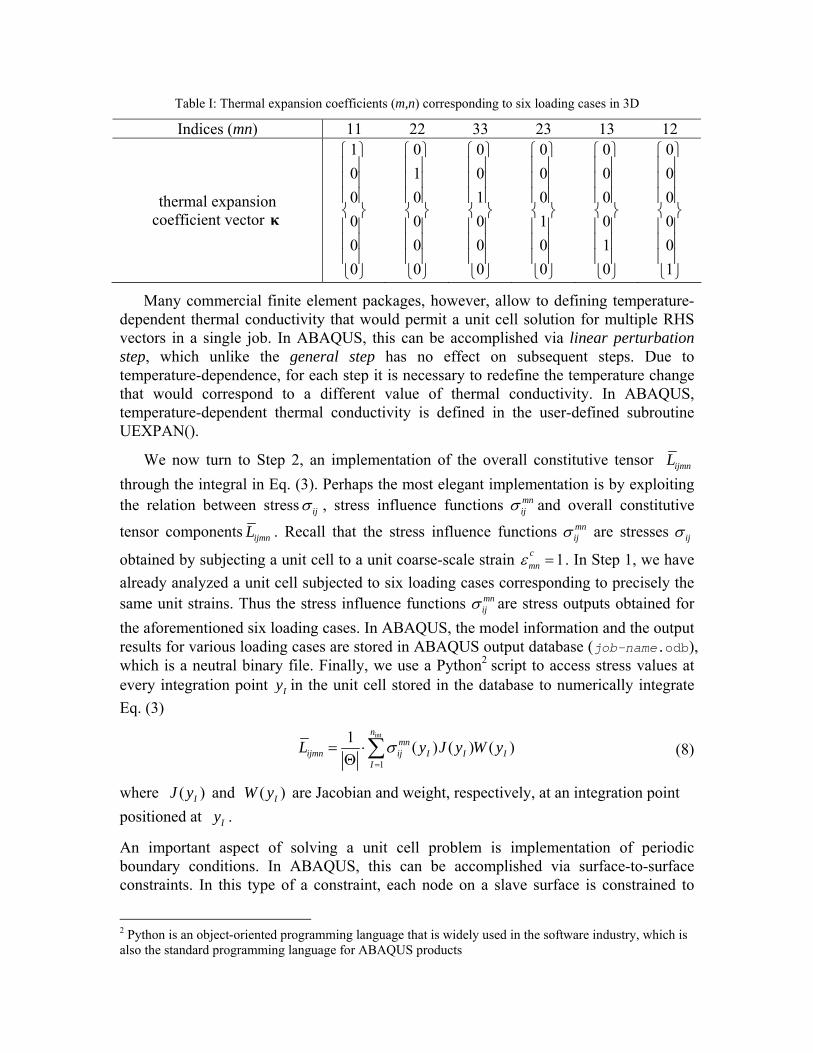
Table I: Thermal expansion coefficients (m,n) corresponding to six loading cases in 3D

Indices (mn) 11 22 33 23 13 12

thermal expansion coefficient vector κ

100000

⎧ ⎫⎪ ⎪⎪ ⎪⎪ ⎪⎨ ⎬⎪ ⎪⎪ ⎪⎪ ⎪⎩ ⎭

010000

⎧ ⎫⎪ ⎪⎪ ⎪⎪ ⎪⎨ ⎬⎪ ⎪⎪ ⎪⎪ ⎪⎩ ⎭

001000

⎧ ⎫⎪ ⎪⎪ ⎪⎪ ⎪⎨ ⎬⎪ ⎪⎪ ⎪⎪ ⎪⎩ ⎭

000100

⎧ ⎫⎪ ⎪⎪ ⎪⎪ ⎪⎨ ⎬⎪ ⎪⎪ ⎪⎪ ⎪⎩ ⎭

000010

⎧ ⎫⎪ ⎪⎪ ⎪⎪ ⎪⎨ ⎬⎪ ⎪⎪ ⎪⎪ ⎪⎩ ⎭

000001

⎧ ⎫⎪ ⎪⎪ ⎪⎪ ⎪⎨ ⎬⎪ ⎪⎪ ⎪⎪ ⎪⎩ ⎭

Many commercial finite element packages, however, allow to defining temperature-dependent thermal conductivity that would permit a unit cell solution for multiple RHS vectors in a single job. In ABAQUS, this can be accomplished via linear perturbation step, which unlike the general step has no effect on subsequent steps. Due to temperature-dependence, for each step it is necessary to redefine the temperature change that would correspond to a different value of thermal conductivity. In ABAQUS, temperature-dependent thermal conductivity is defined in the user-defined subroutine UEXPAN().

We now turn to Step 2, an implementation of the overall constitutive tensor ijmnL through the integral in Eq. (3). Perhaps the most elegant implementation is by exploiting the relation between stress ijσ , stress influence functions mn

ijσ and overall constitutive

tensor components ijmnL . Recall that the stress influence functions mnijσ are stresses ijσ

obtained by subjecting a unit cell to a unit coarse-scale strain 1cmnε = . In Step 1, we have

already analyzed a unit cell subjected to six loading cases corresponding to precisely the same unit strains. Thus the stress influence functions mn

ijσ are stress outputs obtained for the aforementioned six loading cases. In ABAQUS, the model information and the output results for various loading cases are stored in ABAQUS output database (job-name.odb), which is a neutral binary file. Finally, we use a Python2 script to access stress values at every integration point Iy in the unit cell stored in the database to numerically integrate Eq. (3)

int

1

1 ( ) ( ) ( )n

mnijmn ij I I I

IL y J y W yσ

=

= ⋅Θ ∑ (8)

where ( )IJ y and ( )IW y are Jacobian and weight, respectively, at an integration point positioned at Iy .

An important aspect of solving a unit cell problem is implementation of periodic boundary conditions. In ABAQUS, this can be accomplished via surface-to-surface constraints. In this type of a constraint, each node on a slave surface is constrained to

2 Python is an object-oriented programming language that is widely used in the software industry, which is also the standard programming language for ABAQUS products

have the same motion as a closest point on the master surface. The following rules are used to form the master-slave relation. For an element-based master surface, a point on the master surface closest to a slave node is calculated and then used to determine the master node(s) that will be forming the constraint. For example, in Figure 1, nodes 1, 2 and 3 are used to constrain node c; nodes 1 and 2 constrain node a; and node 2 constrains node b. The element shape functions are used to set up the constraints. It is important to note that when master and slave surfaces have different mesh densities, the master surface should be chosen as the surface with a coarser mesh. Moreover, the POSITION TOLERANCE parameter should be set to be greater than the distance between two surfaces (see definition of ABAQUS keyword “*TIE” in online ABAQUS Keywords Reference Manual).

Figure 1: Master-slave relations for an element-based master surface

Finally, the coarse scale analysis is carried out using overall coefficients computed in Step 2. For the postprocessing (Step 4), the coarse scale strains obtained in Step 3 are used in combination with stress influence functions calculated in Step 1 to compute the fine scale stresses in critical (or all) unit cells as

mn cij ij mnσ σ ε= (9)

For verification, we consider a three-dimensional fibrous unit cell. The phase properties of the microstructure are summarized in Table II. The unit cell is discretized with 351 tetrahedral elements as shown in Figure 2.

Table II: Material properties for fibrous unit cell

Materials Young’s Modulus Poisson’s ratio Volume fraction Titanium Matrix 68.9 GPa 0.33 0.733

SiC Fiber 379.2 GPa 0.21 0.267

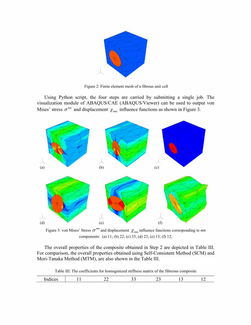
Figure 2: Finite element mesh of a fibrous unit cell Using Python script, the four steps are carried by submitting a single job. The

visualization module of ABAQUS/CAE (ABAQUS/Viewer) can be used to output von Mises’ stress mnσ and displacement imnχ influence functions as shown in Figure 3.

Figure 3: von Mises’ Stress mnσ and displacement imnχ influence functions corresponding to mn

components: (a) 11; (b) 22; (c) 33; (d) 23; (e) 13; (f) 12; The overall properties of the composite obtained in Step 2 are depicted in Table III.

For comparison, the overall properties obtained using Self-Consistent Method (SCM) and Mori-Tanaka Method (MTM), are also shown in the Table III.

Table III: The coefficients for homogenized stiffness matrix of the fibreous composite

Indices 11 22 33 23 13 12

(a) (b) (c)

(d) (e) (f)

140.3 (136.6/134.2)

57.3 (61.8/61.4)

57.7 (57.8/57.3)

0.0 (0.0/0.0)

0.0 (0.0/0.0)

0.1 (0.0/0.0)

140.0 (136.6/134.2)

57.6 (57.8/57.3)

0.0 (0.0/0.0)

0.0 (0.0/0.0)

0.1 (0.0/0.0)

185.6 (185.7/185.6)

0.0 (0.0/0.0)

0.0 (0.0/0.0)

0.0 (0.0/0.0)

39.5 (40.1/38.2)

0.0 (0.0/0.0)

0.0 (0.0/0.0)

SYM. 39.4 (40.1/38.2)

0.0 (0.0/0.0)

FEM Results (GPa)

(SCM/MTM)

36.5 (37.4/36.4)

For the coarse scale analysis in Step 3, we consider a cantilever beam subjected to a uniform distributed load along the top edge. For comparison, a reference solution is obtained using a single scale finite element analysis on a fine mesh. Deformed meshes and von Mises’ stresses at a critical unit cell (left bottom corner) are shown in Figure 4. The stresses in a unit cell are obtained by postprocessing in Step 4.

Figure 4: Comparison of the homogenization and the reference solutions

(a) reference solution (b) homogenization solution

For convenience, all input files, user-defined subroutines and Python script for the above example can be can be found in http://www.rpi.edu/~fishj/***.

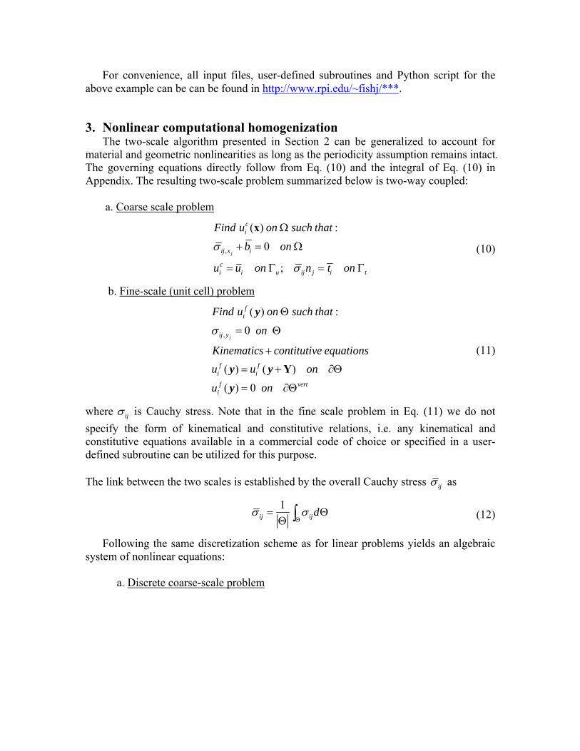
3. Nonlinear computational homogenization The two-scale algorithm presented in Section 2 can be generalized to account for material and geometric nonlinearities as long as the periodicity assumption remains intact. The governing equations directly follow from Eq. (10) and the integral of Eq. (10) in Appendix. The resulting two-scale problem summarized below is two-way coupled: a. Coarse scale problem

,

( ) :

0

;j

ci

ij x i

ci i u ij j i t

Find u on such that

b on

u u on n t on

σ

σ

Ω

+ = Ω

= Γ = Γ

x

(10)

b. Fine-scale (unit cell) problem

,

( ) :

0

( ) ( )

( ) 0

j

fi

ij y

f fi if vert

i

Find u on such that

on

Kinematics contitutive equationsu u on

u on

σ

Θ

= Θ

+

= + ∂Θ

= ∂Θ

Y

y

y yy

(11)

where ijσ is Cauchy stress. Note that in the fine scale problem in Eq. (11) we do not specify the form of kinematical and constitutive relations, i.e. any kinematical and constitutive equations available in a commercial code of choice or specified in a user-defined subroutine can be utilized for this purpose. The link between the two scales is established by the overall Cauchy stress ijσ as

1

ij ijdσ σΘ

= ΘΘ ∫ (12)

Following the same discretization scheme as for linear problems yields an algebraic system of nonlinear equations: a. Discrete coarse-scale problem

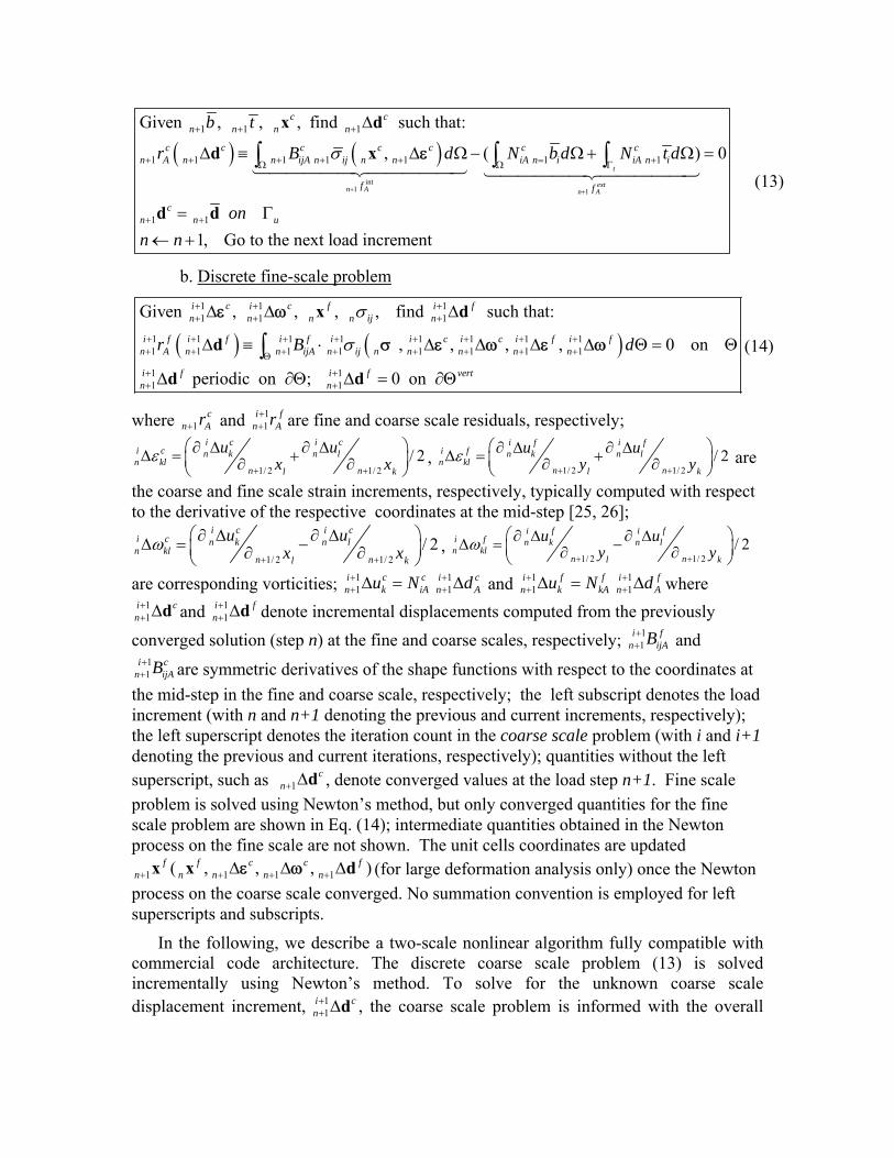
( ) ( )int

1 1

1 1 1

1 1 1 1 1 1 1

1 1

Given , , , find such that:

, ( ) 0

1, Go to the next load inc

t

extn A n A

c cn n n n

c c c c c c cn A n n ijA n ij n n iA n i iA n i

f f

cn n u

b t

r B d N b d N t d

onn n

σ

+ +

+ + +

+ + + + + = +Ω Ω Γ

+ +

Δ

Δ ≡ Δ Ω− Ω+ Ω =

= Γ

← +

∫ ∫ ∫x d

d x

d d

ε

rement

(13)

b. Discrete fine-scale problem

( ) ( )

1 1 11 1 1

1 1 1 1 1 1 1 11 1 1 1 1 1 1 1

1 11 1

Given , , , , find such that:

, , , , 0 on

periodic on ; 0 on

i c i c f i fn n n n ij n

i f i f i f i i c i c i f i fn A n n ijA n ij n n n n n

i f i f vertn n

r B d

σ

σ

+ + ++ + +

+ + + + + + + ++ + + + + + + +Θ

+ ++ +

Δ Δ Δ

Δ ≡ ⋅ Δ Δ Δ Δ Θ = Θ

Δ ∂Θ Δ = ∂Θ

∫x d

d

d d

ε ω

σ ε ω ε ω (14)

where 1c

n Ar+ and 11

i fn Ar++ are fine and coarse scale residuals, respectively;

1/ 2 1/ 2/ 2

i c i ci c n k n ln kl

n nl k

u ux xε

+ +

⎛ ⎞∂ Δ ∂ ΔΔ = +⎜ ⎟∂ ∂⎝ ⎠,

1/ 2 1/ 2/ 2

i f i fi f n k n ln kl

n nl k

u uy yε

+ +

⎛ ⎞∂ Δ ∂ ΔΔ = +⎜ ⎟∂ ∂⎝ ⎠ are

the coarse and fine scale strain increments, respectively, typically computed with respect to the derivative of the respective coordinates at the mid-step [25, 26];

1/ 2 1/ 2/ 2

i c i ci c n k n ln kl

n nl k

u ux xω

+ +

⎛ ⎞∂ Δ ∂ ΔΔ = −⎜ ⎟∂ ∂⎝ ⎠,

1/ 2 1/ 2/ 2

i f i fi f n k n ln kl

n nl k

u uy yω

+ +

⎛ ⎞∂ Δ ∂ ΔΔ = −⎜ ⎟∂ ∂⎝ ⎠

are corresponding vorticities; 1 11 1

i c c i cn k iA n Au N d+ ++ +Δ = Δ and 1 1

1 1i f f i fn k kA n Au N d+ ++ +Δ = Δ where

11

i cn++ Δd and 1

1i fn++ Δd denote incremental displacements computed from the previously

converged solution (step n) at the fine and coarse scales, respectively; 11

i fn ijAB++ and

11

i cn ijAB++ are symmetric derivatives of the shape functions with respect to the coordinates at

the mid-step in the fine and coarse scale, respectively; the left subscript denotes the load increment (with n and n+1 denoting the previous and current increments, respectively); the left superscript denotes the iteration count in the coarse scale problem (with i and i+1 denoting the previous and current iterations, respectively); quantities without the left superscript, such as 1

cn+ Δd , denote converged values at the load step n+1. Fine scale

problem is solved using Newton’s method, but only converged quantities for the fine scale problem are shown in Eq. (14); intermediate quantities obtained in the Newton process on the fine scale are not shown. The unit cells coordinates are updated

1 1 1 1( , , , )f f c c fn n n n n+ + + +Δ Δ Δx x dε ω (for large deformation analysis only) once the Newton process on the coarse scale converged. No summation convention is employed for left superscripts and subscripts.

In the following, we describe a two-scale nonlinear algorithm fully compatible with commercial code architecture. The discrete coarse scale problem (13) is solved incrementally using Newton’s method. To solve for the unknown coarse scale displacement increment, 1

1i cn++ Δd , the coarse scale problem is informed with the overall

Cauchy stress 11

in ijσ++ and the overall instantaneous constitutive tensor 1

1i

n ijmnL++ .These two

quantities are extracted from the corresponding fine scale fields as

( )1 1 1 1 1 11 1 1 1 1 1

1 , , , ,i i i c i c i f i fn ij n ij n n n n n dσ σ+ + + + + ++ + + + + +Θ

= Δ Δ Δ Δ ΘΘ ∫ σ ε ω ε ω (15)

( )1 1 1 1 1 11 1 1 1 1 1

1 , , , ,i i mn i c i c i f i fn ijmn n ij n n n n nL dσ+ + + + + ++ + + + + +Θ

= Δ Δ Δ Δ ΘΘ ∫ σ ε ω ε ω (16)

where ( )1 1 11 1 1, ,i i c i c

n kl n n nσ+ + ++ + +Δ Δσ ε ω and ( )1 1 1

1 1 1, ,i mn i c i cn ij n n nσ+ + ++ + +Δ Δσ ε ω denote Cauchy stress

and the instantaneous Cauchy stress influence functions, respectively. It is important to note that these quantities correspond to converged (equilibrated) unit cell solution, which may or may not represent the converged coarse scale solution. In ABAQUS, the coarse scale analysis is controlled by a user-defined subroutine UMAT(). At each integration point, increment n+1 and iteration i+1, ABAQUS calls UMAT() routine to carry out the following operations: 1. Write ( )1 1

1 1,i c i cn n+ ++ +Δ Δε ω to an external data file;

2. Write current coarse scale element number, integration point number, increment and iteration numbers into an external file; 3. Invoke Python script to prepare and submit the corresponding unit cell job and to calculate the overall quantities 1

1i

n ijσ++ and 11

in ijmnL++ ; and

4. Read 11

in ijσ++ and 1

1i

n ijmnL++ from an external data file.

We now turn to the fine scale problem. It is important to note that for every coarse scale solution ( )1 1

1 1,i c i cn n+ ++ +Δ Δε ω , the discrete unit cell problems (14) are solved using

Newton’s method. Once (independent) Newton’ processes for all unit cell problems (14) converged, the Cauchy stresses and the Cauchy stress influence functions are computed to evaluate the overall Cauchy stress (15) and the overall instantaneous constitutive tensor (16). From the implementation point of view, one needs to address the following two issues: (i) solution of the unit cell problems; and (ii) evaluation of the stress influence functions.

We start with the first issue. A unit cell geometry (or geometries), finite element mesh, boundary conditions and material models are defined in the input file. One may use commercial code library of materials or define a new material using user-defined facilities. For the unit cell analysis in ABAQUS, this step should be defined as a general step.

Unit cell analyzes are carried out incrementally from the converged unit cell solutions (displacements and stresses), which are stored in the restart file (unit-cell-name.stt). In ABAQUS, this is accomplished using ABAQUS keyword “*RESTART, WRITE”. Two sets of restart files are prepared for each unit cell. One that stores the information from the previous converged stress n ijσ ; the second contains the information from the last iteration, which may or may not represent the converged solution for the next increment. Changing the increment number serves as an indication for the first restart file to be

overwritten by the second one. For continuation of analyzes in ABAQUS, a keyword “*RESTART, READ” is used.

The coarse scale strain increment, 11

i cn mnε++ Δ , is imposed in the form of thermal strains

11 κi c

n mn mn Tε++ Δ = ⋅Δ (17)

where the thermal expansion coefficient and temperature change are chosen as 11κ i c

mn n mnε++= Δ and 1TΔ = . In ABAQUS, UEXPAN() is used to define the thermal

conductivity. Depending on material model, stress updates can be carried out in two steps. In step one, stresses are updated by subjecting a unit cell to thermal strains, κmn T⋅Δ , where

11κ i c

mn n mnε++= Δ . This step may include both material and rotational stress updates and it

utilizes algorithms available in the commercial package of choice. In step two, a unit cell is subjected to a constant rotational increment 1

1i cn++ ΔR computed from the incremental

vorticity 11

i cn++ Δω using well-established procedures [25, 26, 27].

We now focus on the second issue, an evaluation of the instantaneous Cauchy stress influence functions 1

1i mn

n ijσ++ . The stress influence functions are evaluated only once the

converged (on the fine scale) unit cell solution is obtained. Let 11 ( )i

n ijmnL++ y and 1

1 ( )i fn ijAB++ y

be components of the instantaneous material properties and symmetric gradient of the shape functions, respectively, both computed for the converged unit cell solution. The influence functions are then obtained by solving a linearized unit cell problem

1 1 1 1 1 11 1 1 1 1 1

1 11 1 ; 0

i f i i f i f i f in ijA n ijst n stB n mnB n ijA n ijst

i f i f vertn mnB n mnB

B L B d d B L d on

d periodic on d on

+ + + + + ++ + + + + +Θ Θ

+ ++ +

Θ ⋅ Δ = − Θ Θ

Δ ∂Θ Δ = ∂Θ

∫ ∫ (18)

for six RHS vectors. This step is similar to Step 1 in linear homogenization discussed in Section 2. It is important to emphasize, however, that Eq. (18) is a linear perturbation step with fixed 1

1i

n ijmnL++ (see Remark below). The unit cell displacements 1

1i fn mnBd++ Δ obtained

and the influence functions

( )1 1 1 11 1 1 1ˆi mn i i f i f

n ij n ijkl n mnB n klB klmnL B d Iσ+ + + ++ + + += Δ + (19)

have no influence on the unit cell solutions in subsequent increments and/or iterations of the coarse scale problem.

The stress influence functions computed in Eq. (19) are free of coarse scale incremental rotation 1

1i cn++ ΔR . One may proceed to defining the corotational overall

constitutive tensor 11

ˆin ijmnL++ , which is free of the coarse scale incremental rotation

( )1 1 1 1 1 11 1 1 1 1 1

1ˆ ˆ , , 0, ,i i mn i c i c i f i fn ijmn n ij n n n n nL dσ+ + + + + ++ + + + + +Θ

= Δ Δ = Δ Δ ΘΘ ∫ σ ε ω ε ω

followed by an appropriate rotation of 11

ˆin ijmnL++ to the global coordinate system.

The flowchart illustrating the key implementation steps including the reference to the source files (available online at http://www.rpi.edu/~fishj/***) and ABAQUS commands at each step are depicted in Figure 5. Remark 1: For user-defined inelastic material models, the instantaneous material properties 1

1i

n ijmnL++ are automatically stored in ABAQUS database, and therfore Eq. (19)

can be computed as a linear perturbation step. For inelastic material models within ABAQUS library the instantaneous material properties 1

1i

n ijmnL++ are not accessible to the

user, and therefore, a linear perturbation step cannot be performed unless the converged step corresponds to elastic process (see [26] for definition of elastic and inelastic processes). In this case one has to carry out six general perturbation steps instead. A general perturbation step is defined with an infinitesimal increment of coarse scale strain and large convergence tolerance so that only a single iteration on the fine scale is carried out.

Coarse Scale Analysis

Command: abaqus job=global user=uglobalMAT.for int

Input File: global.inp

Stress Update Procedure

Command invoke the Python script: CALL SYSTEM ("abaqus cae noGUI=UCP.py")

User-defined Subroutine UMAT(): uglobalMAT.for

Quantities write out: ( )1 11 1,i c i c

n n+ ++ +Δ Δε ω

Quantities read in: 11

in ijσ++ and 1

1i

n ijmnL++

Two Scale Bridging

Python Script: UCP.py

Command execute fine scale analysis: os.system( "".join( [ "abaqus job=",localname, "

input=",inplocalname, " oldjob=", oldlocalname, " int" ] ) )

Preparation for fine scale analysis: Determine the restarting point;

11 �i c

n mn mn Tε++ Δ = ⋅Δ

Calculation of the overall quantites: 1 1 01 1

1 11 1

1

1

i in ij n ij

i i mnn ijmn n ij

d

L d

σ σ

σ

+ ++ +Θ

+ ++ +Θ

= ΘΘ

= ΘΘ

∫

∫

Fine Scale Analysis

Input Files: local*.inp

User-defined Subroutine UEXPAN(): ulocalsubs.for

One general step for ( )1 1 11 1 1, ,i i c i c

n kl n n nσ+ + ++ + +Δ Δσ ε ω

Six perturbation steps for ( )1 1 11 1 1, ,i mn i c i c

n ij n n nσ+ + ++ + +Δ Δσ ε ω

Figure 5: Program architecture for the two-scale analysis using ABAQUS

For verification, we consider several examples. The first two consider a coarse scale domain in the shape of a block discretized with a single brick element subjected to transverse tension. On the fine scale, we consider a fibrous unit cell introduced in Section 2 obeying perfect plasticity for the matrix phase ( 24Y MPaσ = ) and linear elasticity for the fiber phase. The overall response of the composite is obtained using computational framework presented in this section. The overall stress-strain curve along the loading directions is shown in Figure 6 (the reference solution is obtained using a single scale analysis with a fine mesh). The relevant files for this example can be downloaded from http://www.rpi.edu/~fishj/***.

0.00E+00

1.00E+07

2.00E+07

3.00E+07

4.00E+07

5.00E+07

6.00E+07

0.00 0.10 0.20 0.30 0.40 0.50 0.60 0.70 0.80 0.90 1.00

Strain E11 (*E-03)

Stre

ss S

11 (P

a)

REFHOMO

Figure 6: xx xxσ ε− relation for the transverse tension problem with matrix obeying plasticity model

It is important to note that the algorithms presented here are independent of material model considered. For the second example, we keep the same geometry, mesh and boundary conditions, but model the matrix phase using continuum damage mechanics model with arctangent form of damage evolution law [27]. The resulting overall stress-strain curve is shown in Figure 7.

0.00E+00

5.00E+06

1.00E+07

1.50E+07

2.00E+07

2.50E+07

3.00E+07

3.50E+07

0.00 0.10 0.20 0.30 0.40 0.50 0.60 0.70 0.80 0.90 1.00

Strain E11 (*E-03)

Stre

ss S

11 (P

a)

REFHOMO

Figure 7: xx xxσ ε− relation for the transverse tension problem with matrix obeying damage model

For the final example, we simulate crack propagation in a rectangular plate made of a woven composite microstructure [ 28 ]. A quarter of the plate is considered due to symmetry. A uniformly distributed tensile load is applied along the top edge. Continuum damage model considered in the previous example is employed. The value of damage parameter ( 1 fully crackedω = ) governs crack formation. Crack propagation obtained with the two-scale homogenization and the reference solution obtained with a single finite element mesh containing over one half million of elements are depicted in Figures 9 and 8, respectively. Figure 10 compares the crack length obtained by the two methods. The two-scale homogenization performs fairly well considering the fact that solution periodicity in the vicinity of the crack does not exist.

Figure 8: Crack propagation using single scale finite element analysis (reference solution)

Figure 9: Crack propagation in the coarse scale model

0 0.05 0.1 0.15 0.2 0.250

0.5

1

1.5

2

2.5

3

3.5

4

4.5

5

Time

Cra

ck le

ngth

(# o

f uni

t cel

l len

gth)

ReferenceHomogenization

Figure 10: Crack length versus time

4. Summary and future research direction We have demonstrated that computational homogenization is fully compatible with conventional finite element code architecture. Once all the input files, user-defined subroutines and Python script are in place, the two-scale analysis can be executed with a single “push button.” We hope that the manuscript will motivate practitioners to adopt the computational homogenization as an integral part of the analysis and design process. We also hope that commercial code vendors will seamlessly integrate the architectures proposed in their legacy codes. The issue of computational cost of the two-scale nonlinear analysis has not been addressed in the present manuscript. As one may expect, the cost is very high indeed. Let

cellsN be the number of Gauss points in the coarse scale, n be the number of load increments in the coarse scale, coarseI and fineI be the average number of iterations in the coarse and fine scales respectively. Then the total number of linear solves of the fine scale problem is cells coarse fineN n I I⋅ ⋅ ⋅ , certainly a formidable computational cost if the number of unit cells and degrees-of-freedom in a unit cell is substantial.

(b) Overall stress component yyσ (a) Overall damage parameter

We believe that it is a combination of two remedies that will eventually reduce the computational cost to a manageable size. The first is utilization of parallel computing since unit cell computations are fully parallelizable. The second is coarse-graining or model reduction. Some (but not all) noteworthy efforts in this direction have been mentioned in the introduction of this paper [11-22]. In our upcoming manuscript [29], we will demonstrate how one specific model reduction approach can be seamlessly integrated into commercial finite element code architecture.

Acknowledgment The financial supports of National Science Foundation under grants CMS-0310596, 0303902, 0408359, Rolls-Royce contract 0518502, Automotive Composite Consortium contract 606-03-063L, and AFRL/MNAC MNK-BAA-04-0001 contract are gratefully acknowledged. The authors wish to thank Prof. Terada for his constructive suggestions. Appendix: Mathematical homogenization for linear elasticity The strong form of the boundary value problem for linear elastostatics is given by

, 0jij x ib onζ ζσ + = Ω (1)

ij ijkl klL onζ ζ ζ ζσ ε= Ω (2)

( , ) , ,( ) / 2l l kkl k x k x l xu u u onζ ζ ζ ζ ζε ≡ = + Ω (3)

i i uu u onζ = Γ (4)

ij j i tn t onζσ = Γ (5)

Eqs. (1)-(5) are equilibrium equations, constitutive relations, kinematical relations, displacement boundary conditions and traction boundary conditions. The superscript ζ denotes Y-periodicity of the corresponding function f , i.e. ( ) ( ), ,f k f+ =Yx y x y , where Y is the characteristic size of the fine scale (unit cell), and k is a non-zero integer.

A two-scale asymptotic expansion is employed to approximate the displacement field

0 1 2 2( ) ( , ) ( , )i i i iu u u uζ ζ ζ= + + +x, y x y x y (6)

where ( )iu x, y are Y-periodic functions, for 0,1,2,...= . Using the chain rule of the differentiation ( ) 1

, , ,,i i ix x yf f fζ −= +x y , and kinematical

relations Eq. (3), the asymptotic expansion of the strain field is given as

1 1 0 0 1 1( ) ( , ) ( , )kl kl kl klζε ζ ε ζ ε ζ ε− −= + + +x, y x y x y (7)

where,

( ) ( )

1 0

0 0 1, ,

1 1 2

; 0,1, 2,...l l

kl kly

kl klx kly klx klyk x k y

kl klx kly

and u u for

ε ε

ε ε ε ε ε

ε ε ε

−⎧ =⎪⎪ = + = = =⎨⎪

= +⎪⎩

The asymptotic expansion of the stress field is

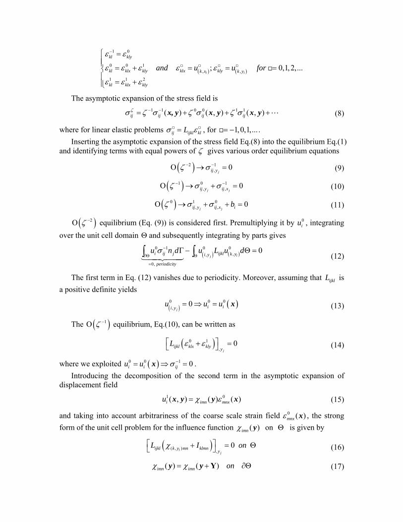
1 1 0 0 1 1( ) ( , ) ( , )ij ij ij ijζσ ζ σ ζ σ ζ σ− −= + + +x, y x y x y (8)

where for linear elastic problems ij ijkl klLσ ε= , for 1,0,1,...= − . Inserting the asymptotic expansion of the stress field Eq.(8) into the equilibrium Eq.(1)

and identifying terms with equal powers of ζ gives various order equilibrium equations

( )2 1, 0

jij yζ σ− −Ο → = (9)

( )1 0 1, , 0

j jij y ij xζ σ σ− −Ο → + = (10)

( )0 1 0, , 0

j jij y ij x ibζ σ σΟ → + + = (11)

( )2ζ −Ο equilibrium (Eq. (9)) is considered first. Premultiplying it by 0iu , integrating

over the unit cell domain Θ and subsequently integrating by parts gives

( ) ( )0 1 0 0

,,

0,

0lj

i ij j ijkl k yi y

periodicity

u n d u L u dσ −

∂Θ Θ

=

Γ − Θ =∫ ∫ (12)

The first term in Eq. (12) vanishes due to periodicity. Moreover, assuming that ijklL is a positive definite yields

( ) ( )0 0 0,

0j

i ii yu u u= ⇒ = x (13)

The ( )1ζ −Ο equilibrium, Eq.(10), can be written as

( )0 1

,0

jijkl klx kly y

L ε ε⎡ ⎤+ =⎣ ⎦ (14)

where we exploited ( )0 0 1 0i i iju u σ −= ⇒ =x . Introducing the decomposition of the second term in the asymptotic expansion of

displacement field

1 0( , ) ( ) ( )i imn mnxu χ ε=x y y x (15)

and taking into account arbitrariness of the coarse scale strain field 0 ( )mnxε x , the strong form of the unit cell problem for the influence function ( )imnχ y on Θ is given by

( )( , ) ,0

lj

ijkl k y mn klmn yL I onχ⎡ ⎤+ = Θ⎣ ⎦ (16)

( ) ( )imn imn onχ χ= + ∂ΘYy y (17)

( ) 0 vertimn onχ = ∂Θy (18)

where ( ) / 2klmn mk nl nk mlI δ δ δ δ= + ; vert∂Θ are the vertices of the unit cell. Eq.(18) is often

replaced by the normalization condition 0imndχΘ

Θ =∫ .

Finally, substituting constitutive relations for 0ijσ into equilibrium Eq.(11) yields

( )( )1 0, ,, 0

j jlij y ijkl klmn mnx x ik y mnL I bσ χ ε+ + + = (19)

Integrating Eq.(19) over the unit cell domain and accounting for the periodicity of 1ijσ

yields

0, 0

jijmn mnx x iL bε + = (20)

where

( )( ),1

1

lijmn ijkl klmnk y mn

i i

L L I d

b b d

χΘ

Θ

= + ΘΘ

= ΘΘ

∫

∫

Remark 2: In Sections 2 and 3 we adopted the following nomenclature 0 0 0 1, , ,c c f

ij ij mn mnx i i i iu u u uσ σ ε ε≡ ≡ = =

which is more transparent to readers that are not familiar with nomenclature of the mathematical homogenization.

5. References 1 E-Composites, Inc, “Global Composites Markets 2004-2010” Report, 5679 Bayberry Farms Dr., SW, Grandville, MI 49418, USA 2 J.D. Eshelby, “The determination of the field of an ellipsoidal inclusion and related problems,” Proc. R. Soc. Lond. A, Vol. 241, pp. 376-396, (1957) 3 Z. Hashin, “ The elastic moduli of heterogeneous materials,” J. Appl. Mech., Vol. 29, pp. 143-150, (1962) 4 T. Mori and K. Tanaka, “Average stress in the matrix and average elastic energy of materials with misfitting inclusions,” Acta Metall., Vol. 21, pp. 571-574, (1973). 5 R. Hill, “A self-consistent mechanics of composite materials,” J. Mech. Phys. Solids, Vol. 13, pp. 357-372, (1965) 6 R. M. Christensen and K.H. Lo, “Solution for effective shear properties in three phase sphere and cylinder models,” J. Mech. Phys. Solids, Vol. 27, pp. 315-330, (1979). 7 A. Benssousan, J.L. Lions and G. Papanicoulau, “Asymptotic Analysis for Periodic Structures”, North-Holland, 1978. 8 E. Sanchez-Palencia, “Non-homogeneous media and vibration theory,” Lecture notes in physics, Vol. 127, Springer-Verlag. Berlin. (1980).

9 J. M. Guedes and N. Kikuchi, “Preprocessing and postprocessing for materials based on the homogenization method with adaptive finite element methods”, Computer Methods in Applied Mechanics and Engineering, Vol. 83, pp. 143-198, 1990. 10 Terada, K., and Kikuchi, N., “Nonlinear homogenization method for practical applications”, Computational Methods in Micromechanics, S. Ghosh and M. Ostoja-Starzewski (eds.), ASME, New York, Vol. AMD-212/MD-62, pp. 1-16, 1995. 11 J. Fish, K. Shek, M. Pandheeradi, and M.S. Shephard, “Computational Plasticity for Composite Structures Based on Mathematical Homogenization: Theory and Practice”, Comp. Meth. Appl. Mech. Engng., Vol. 148, pp. 53-73, 1997. 12 J. Fish and K. L. Shek, “Finite Deformation Plasticity of Composite Structures: Computational Models and Adaptive Strategies”, Comp. Meth. Appl. Mech. Engng., Vol. 172, pp. 145-174, 1999. 13 J. Fish and Q.Yu, “Multiscale Damage Modeling for Composite Materials: Theory and Computational Framework”, International Journal for Numerical Methods in Engineering, Vol. 52, No 1-2, pp. 161-192 2001. 14 Terada, K., and Kikuchi, N., “A class of general algorithms for multi-scale analysis of heterogeneous media”, Comput. Methods Appl. Mech. Eng. 190:5427-5464, 2001. 15 K. Matsui, K. Terada and K. Yuge, “Two-scale finite element analysis of heterogeneous solids with periodic microstructures”, Computers and Structures 82 (7-8), pp. 593-606, 2004. 16 Smit, R.J.M., Brekelmans, W.A.M., and Meijer, H.E.H., “Prediction of the mechanical behavior of nonlinear heterogeneous systems by multilevel finite element modeling”, Comput. Methods Appl. Mech. Eng. 155:181-192, 1998. 17 Miehe, C., and Koch, A., “Computational micro-to-macro transition of discretized microstructures undergoing small strain”, Arch. Appl. Mech. 72:300-317, 2002. 18 Kouznetsova, V., Brekelmans, W.-A., and Baaijens, F.P.-T., “An approach to micro-macro modeling of heterogeneous materials”, Comput. Mech. 27:37-48, 2001. 19 Feyel, F., and Chaboche, J.-L., “FE2 multiscale approach for modeling the elastoviscoplastic behavior of long fiber sic/ti composite materials”, Comput. Methods Appl. Mech. Eng. 183:309-330, 2000. 20 Ghosh, S., Lee, K., and Moorthy, S., “Multiple scale analysis of heterogeneous elastic structures using homogenization theory and Voronoi cell finite element method”, Int. J. Solids Struct. 32:27-62, 1995. 21 Ghosh, S., Lee, K., and Moorthy, S. “Two scale analysis of heterogeneous elasticplastic materials with asymptotic homogenization and Voronoi cell finite element model”. Comput. Methods Appl. Mech. Engrg., 132:63-116, 1996. 22 Michel, J.-C., Moulinec, H., and Suquet, P., “Effective properties of composite materials with periodic microstructure: a computational approach”, Comput. Methods Appl. Mech. Eng. 172:109-143, 1999. 23 M.G.D. Geers, V. Kouznetsova, W.A.M. Brekelmans, “Gradient-enhanced computational homogenization for the micro-macro scale transition,” J. Phys. IV, Vol. 11, pp. 145-152 (2001) 24 C. McVeigh, F. Vernerey, W. K. Liu, L. C. Brinson, “Multiresolution analysis for material design,” Comput. Methods Appl. Mech. Engrg. Vol. 195, pp. 5053–5076, 2006. 25 T. Belytschko, W.K. Liu, B. Moran, “Nonlinear Finite Elements for Continua and Structures,” John Wiley and Sons Ltd, (2003) 26 J.C. Simo and T.J.R. Hughes, “Computational Inelasticity,” in Interdisciplinary Applied Mathamitics, Vol. 7. Springer-Verlag, New-York, (1998) 27 Fish, J., Yu, Q., and Shek, K. “Computational damage mechanics for composite materials based on mathematical homogenization”, Int. J. Numer. Meth. Engrg., 45:1657-1679, 1999. 28 R. Wentorf, R. Collar, M.S. Shephard, J. Fish, “Automated Modeling for Complex Woven Mesostructures,” Computer Methods in Applied Mechanics and Engineering, Vol. 172, pp. 273-291, 1999. [29] C. Oskay and J. Fish, “A model reduction approach for failure analysis of periodic heterogeneous media,” submitted to Computer Methods in Applied Mechanics and Engineering, (2006).