Computational Analysis of Two-Phase flow in Horizontal

International Research Journal of Engineering and Technology (IRJET) e-ISSN: 2395-0056

Volume: 07 Issue: 08 | Aug 2020 www.irjet.net p-ISSN: 2395-0072

© 2020, IRJET | Impact Factor value: 7.529 | ISO 9001:2008 Certified Journal | Page 4450

Computational Analysis of Two-Phase flow in Horizontal Pipeline

Mohamed Abul Z1, Manish MU2, Padmanathan P3, Vignesh P4, Satheesh A5

1Bachelor of Mechanical Engineering, Vellore Institute of Technology, Vellore-632014 2Bachelor of Mechanical Engineering, Vellore Institute of Technology, Vellore-632014

3Assistant Professor Sr. Grade, School of Mechanical Engineering, Vellore Institute of Technology, Vellore-632014, Tamil Nadu, India

---------------------------------------------------------------------***---------------------------------------------------------------------

Abstract - CFD analysis of non-boiling two-phase flow of Air-Water and Vapour-Oil in horizontal pipeline were done. ANSYS Design modular was used to develop the geometry and mesh for horizontal pipe and then transfer the data to Fluent for further analysis. The pipe of 8 mm inner diameter and 2m of length is taken. The simulation was carried out under adiabatic condition and operating at normal temperature which was 298 K and atmospheric pressure of 101,325 Pa. Effects of gravitation was considered. Eulerian- Multi-fluid Volume of Fluid (VOF) model and standard K-ɛ turbulence has been employed. For producing more conclusive result, two separate two-phase flow of Air-Water and Vapour-Oil are taken. Stratified, wavy, slug and annular flow are generated and the obtained contours were compared to validate the works of Schepper et al. 2007, Rahimi et al. 2013 and Ban et al. 2017. Pressure drop is an important parameter to take into account for studying pipe flow. The obtained pressure drop from CFD is compared with the standard pressure drop correlations among which Friedel (1979) stands out to be the more suitable model. Turbulence Kinetic Energy of the flow was studied for different fluids and flow regimes.

Key Words: Two-phase; Non-boiling; Horizontal; Pipe flow; Eulerian; Flow regimes; Pressure drop; Pressure drop correlations; Turbulence kinetic energy.

1. INTRODUCTION This Multiphase flow is a widely faced phenomenon in the nature and various industrial applications. It is frequently encountered in long distance pipelines (oil and natural gas), power generation (steam and water), petrochemical and process plants. Two-phase flow is a case of multiphase flow where two phases are involved. Liquid-Gas, Liquid-solid and Gas-solid are some of the two phase flows.

Two-phase flow regimes are investigated for selecting the suitable flow pattern to minimize the pressure loss in transportation of gas and liquid phases. Extraction of water or liquid petroleum is practically done using gas from underground. For improved efficiency, maximum quantity of liquid is to be extracted per unit energy.

The study of two-phase pressure drop is an importance parameter in the design of various engineering applications such as chemical, pharmaceutical, petroleum, nuclear, refrigeration and air conditioning systems.

Numerous results are developed by previous researchers on two-phase flow but there was no reported work for CFD simulation of horizontal pipe flow using Eulerian model. Pressure drop study for each different flow regime was also unavailable. Guerrero et al. [1] conducted a comparison between two CFD models Eulerian and VOF model in an upward flow. As a result, the Eulerian model shows mean square errors (13.86%) lower than the VOF model (19.04%) for low void fraction flows (< 0.25). Schepper et al. [4] compared Vapour–liquid two-phase horizontal flow regimes with experimental data, taken from the Baker chart. V.Jagan, A.Satheesh [11] The experimental investigation of two-phase flow behaviour in a pipe with different orientations is presented in the study. Image processing technique is used to calculate the void fraction percentage. The influence of the angle of pipe inclination on flow pattern maps and void fraction is presented. C.Rajesh Babu[2] tested the model two-phase (water+air) flow in turbulent conditions .The numerical method is FDM approach(Finite difference method). Upwind Discretization scheme is used for this project. Flow regime identification through visualization, Pressure drop measurement are calculated.

Archibong-Eso et al. [6] conducted highly viscous oil-water two-phase flow in pipeline for superficial velocities of oil and water 0.06 m/s to 0.55 m/s and 0.01 m/s to 1.0 m/s. Pressure gradients were used for measure the axial pressure measurement. Flow pattern determination was aided by high definition video recording. P.Bhramara et al.[5] conducted a CFD analysis on refrigerants and compared the pressure drop with standard correlations. Mazumder et al. [9] performed CFD analysis for a two-phase air-water flow through a horizontal to vertical 90° elbow. To analyze the flow behaviour in the elbow, pressure and velocity profiles at six different upstream and downstream locations of the elbow were compared. CFD examination results indicated a reduction in pressure as liquid leaves the elbow notwithstanding a bigger pressure drop at higher air speeds.

Perez et al.[8] used CFD approach to simulate air-highly viscous oil two-phase slug flow. The Volume of Fluid method, the Continuum Surface Force (CSF) model and the High Resolution Interface Capturing (HRIC) scheme were utilized.

Velocity profile is not fully developed near the bottom of slug body. Cacho [7] performed various correlations for analysing two-phase models and estimating pressure gradient in geothermal wellbore application. The accuracy of the




correlation varies with the condition of fluid and its flow regime. Darzi-Park[10] Horizontal two-phase flow is more complex than vertical two-phase flow since the flow is not axis symmetric, due to the gravity. The observed flow patterns of stratified, wavy, plug and slug flows were found to be generally consistent with Mandhane’s flow map except annular flow which was observed at relatively lower gas superficial velocities and also wavy flows were obtained for relatively higher water superficial velocities in the experiment.

Ban et al. [12] The interfacial behaviors of two-phase flow is simulated and compared with experimental data. Due to unsteady nature of slug flow, the translational slug velocity varied along the pipe is difficult to be measured accurately. For a constant superficial liquid velocity the translational slug velocity increased with increasing gas superficial velocity.

Furthermore, Correlations for liquid holdup and slug frequency by comparison are proposed. The predictive models were proposed for calculating pressure gradient, liquid holdup and slug frequency. Pressure gradient increases with increasing gas superficial velocity at liquid superficial velocity. Whereas slug liquid holdup decreased with increasing gas superficial velocity. Liu et al. [13] Turbulence Modelling: Reynolds Stress Model over k- epsilon for liquid-liquid cylindrical cyclone. In Fluent we can use Euler- Lagrange and Euler-Euler approach for Multiphase Modelling. For validation the experiment on oil and water being compared with Air and water for the same geometry.

1.1 Objective

The investigation will be carried out using CFD to analyse the two-phase flow using Eulerian- Multifluid (VOF) model for Air-Water and Vapour-oil mixture. The flow maps obtained will be compared with the previous works to validate the Baker’s chart application for thin pipes. An intensive study of pressure variation along the flow is conducted. Pressure drop will be calculated and validated with standard pressure drop correlation model. The variation of turbulent kinetic energy along pipe is studied and monitored.

1.2 Governing equations

The flow model is governed by conservation of mass, momentum and energy equations in the control volume. The below governing equations are solved for the multiphase flow model.

(1)

(2)

Volume Fraction (∝k) is the ratio of the volume of kth phase to the volume of two phase mixture. In each control volume, the sum of volume fractions of all phases is unity.

(3) The quality or dryness fraction of the two-phase fluid is the ratio of the mass of the vapour phase to the total mass of liquid and vapour phase.

(4) Superficial velocity (Usk) of the phase ‘k’ is the flow rate of the phase per unit area.

(5)

Mass flux (Gsk) is the mass flow rate of phase ‘k’ per unit area

(6)

1.3 Pressure drop correlations

The pressure drop of two-phase flow along the pipe is

calculated using CFD and compared with standard

correlations mentioned below.

Homogenous model: The homogenous two-phase flow model

is a separated flow model. The two phases move at equal

velocities and mix together and therefore can be considered

as a quasi-single phase having average fluid properties

depending on mass quality. The model is derived from

continuity and momentum equations.

The average fluid properties can be calculated using

following relations. For average density,

(7)

where x is dryness fraction.

Average viscosity is calculated as below

(8)

Friction factor

(9)




The obtained quantities are substituted in the following

relation to obtain pressure drop

(10)

Where,

G is the total mass flux(Kg/m2-s)

L is the total length of pipe in meter (m)

d is the diameter of pipe in meter (m)

is the two phase friction factor

Lockhart-Martinelli model: Lockhart-Martinelli (L-M) model is a separated flow model and widely used because of its simplicity although it has relatively low accuracy. The following properties are required for calculating L-M pressure model. Reynolds number (Re)

(11) Liquid and Vapour pressure drop

(11)

(12) X coefficient

(13) Two phase pressure gradient multiplier

(14)

Table -1: Lockhart Martinelli’s parameter C

Liquid Vapour C Turbulent Turbulent 20 Laminar Turbulent 12 Turbulent Laminar 10 Laminar Laminar 5

Total frictional pressure drop

(15) Friedel correlation: Correlation is based on average homogeneous density and vapour quality. Two phase density

(16) Parameters: E, F, H

(17)

(18)

(19) Two phase pressure gradient multiplier

(20) where Froude number and Weber number is given below

(21)

(22) Total frictional pressure drop

Chrisholm model:




(23) B Parameter:

For Y< 9.5; B = (24) For 9.5< Y <28;

(25)

For Y>28; B = (26) Two phase pressure gradient model

(27) Total frictional pressure drop

Muller Steinhagen–Heck Correlation:

(28)

(29)

G-coefficient G = A + 2(B-A) x (30)

Frictional Pressure drop

(31)

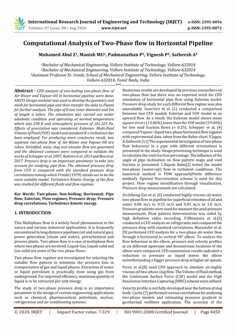
2. GEOMETRY AND MESHING Pipe dimension of diameter 2 meter and width 8 millimetre is taken for the study (L/D=250) used by V Jagan et al. 2016[14]. ANSYS Design Modular 16.0 is used for geometry and meshing. The simulation is done using a 3-D model.

Fig -1: Three-dimensional meshing of the flow pipe

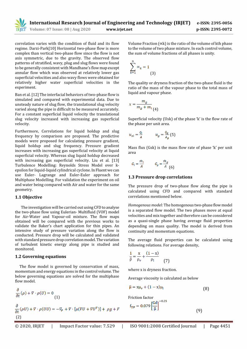
Fig -2: Side view of the mesh For the given geometry, mesh is generated. Orthogonal quality of the worst cells is closer to 0, with the best cells closer to 1. The minimum orthogonality of the mesh is 0.82. Proximity and Curvature is enabled. Coarse mesh is generated. Smooth transition inflation with growth rate of 1.2 is obtained.

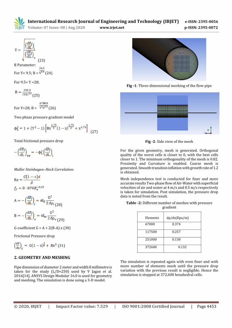
Mesh independence test is conducted for finer and more accurate results Two-phase flow of Air-Water with superficial velocities of air and water at 4 m/s and 0.5 m/s respectively is taken for simulation. Post simulation, the pressure drop data is noted from the result.

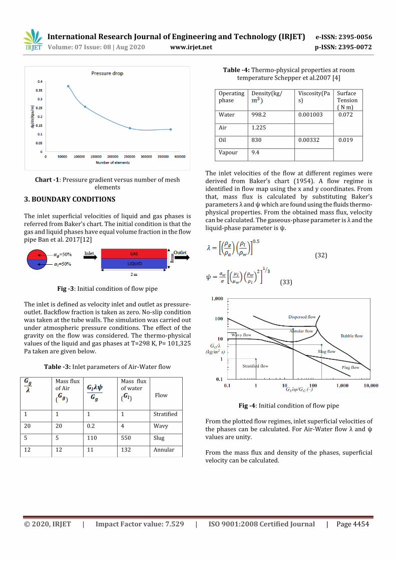
Table -2: Different number of meshes with pressure gradient

Elements

dp/dz(Kpa/m)

67000 0.374

117500 0.257

251000 0.138

372600 0.132

The simulation is repeated again with even finer and with more number of elements mesh until the pressure drop variation with the previous result is negligible. Hence the simulation is stopped at 372,600 hexahedral cells.




Chart -1: Pressure gradient versus number of mesh elements

3. BOUNDARY CONDITIONS The inlet superficial velocities of liquid and gas phases is referred from Baker’s chart. The initial condition is that the gas and liquid phases have equal volume fraction in the flow pipe Ban et al. 2017[12]

Fig -3: Initial condition of flow pipe The inlet is defined as velocity inlet and outlet as pressure-outlet. Backflow fraction is taken as zero. No-slip condition was taken at the tube walls. The simulation was carried out under atmospheric pressure conditions. The effect of the gravity on the flow was considered. The thermo-physical values of the liquid and gas phases at T=298 K, P= 101,325 Pa taken are given below.

Table -3: Inlet parameters of Air-Water flow

Table -4: Thermo-physical properties at room temperature Schepper et al.2007 [4]

Operating phase

Density(kg/

Viscosity(Pa s)

Surface Tension ( N m)

Water 998.2 0.001003 0.072

Air 1.225

Oil 830 0.00332 0.019

Vapour 9.4

The inlet velocities of the flow at different regimes were derived from Baker’s chart (1954). A flow regime is identified in flow map using the x and y coordinates. From that, mass flux is calculated by substituting Baker’s parameters λ and ψ which are found using the fluids thermo-physical properties. From the obtained mass flux, velocity can be calculated. The gaseous-phase parameter is λ and the liquid-phase parameter is ψ.

(32)

(33)

Fig -4: Initial condition of flow pipe From the plotted flow regimes, inlet superficial velocities of the phases can be calculated. For Air-Water flow λ and ψ values are unity. From the mass flux and density of the phases, superficial velocity can be calculated.

Mass flux of Air

( )

Mass flux of water

( )

Flow

1 1 1 1 Stratified

20 20 0.2 4 Wavy

5 5 110 550 Slug

12 12 11 132 Annular




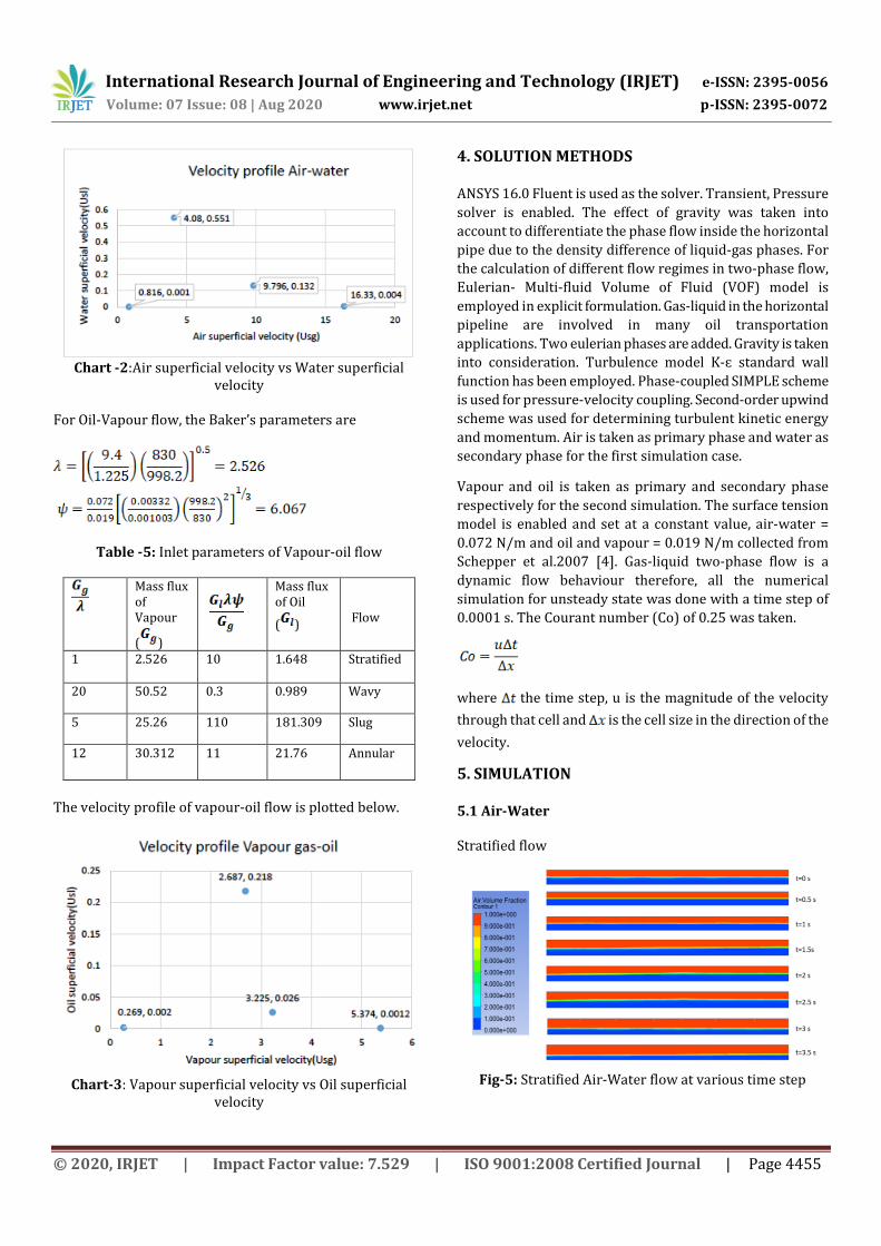
Chart -2:Air superficial velocity vs Water superficial

velocity For Oil-Vapour flow, the Baker’s parameters are

Table -5: Inlet parameters of Vapour-oil flow

Mass flux of Vapour

( )

Mass flux of Oil

( )

Flow

1 2.526 10 1.648 Stratified

20 50.52 0.3 0.989 Wavy

5 25.26 110 181.309 Slug

12 30.312 11 21.76 Annular

The velocity profile of vapour-oil flow is plotted below.

Chart-3: Vapour superficial velocity vs Oil superficial

velocity

4. SOLUTION METHODS ANSYS 16.0 Fluent is used as the solver. Transient, Pressure

solver is enabled. The effect of gravity was taken into

account to differentiate the phase flow inside the horizontal

pipe due to the density difference of liquid-gas phases. For

the calculation of different flow regimes in two-phase flow,

Eulerian- Multi-fluid Volume of Fluid (VOF) model is

employed in explicit formulation. Gas-liquid in the horizontal

pipeline are involved in many oil transportation

applications. Two eulerian phases are added. Gravity is taken

into consideration. Turbulence model K-ɛ standard wall

function has been employed. Phase-coupled SIMPLE scheme

is used for pressure-velocity coupling. Second-order upwind

scheme was used for determining turbulent kinetic energy

and momentum. Air is taken as primary phase and water as

secondary phase for the first simulation case.

Vapour and oil is taken as primary and secondary phase

respectively for the second simulation. The surface tension

model is enabled and set at a constant value, air-water =

0.072 N/m and oil and vapour = 0.019 N/m collected from

Schepper et al.2007 [4]. Gas-liquid two-phase flow is a

dynamic flow behaviour therefore, all the numerical

simulation for unsteady state was done with a time step of

0.0001 s. The Courant number (Co) of 0.25 was taken.

where the time step, u is the magnitude of the velocity

through that cell and is the cell size in the direction of the

velocity.

5. SIMULATION 5.1 Air-Water

Stratified flow

Fig-5: Stratified Air-Water flow at various time step




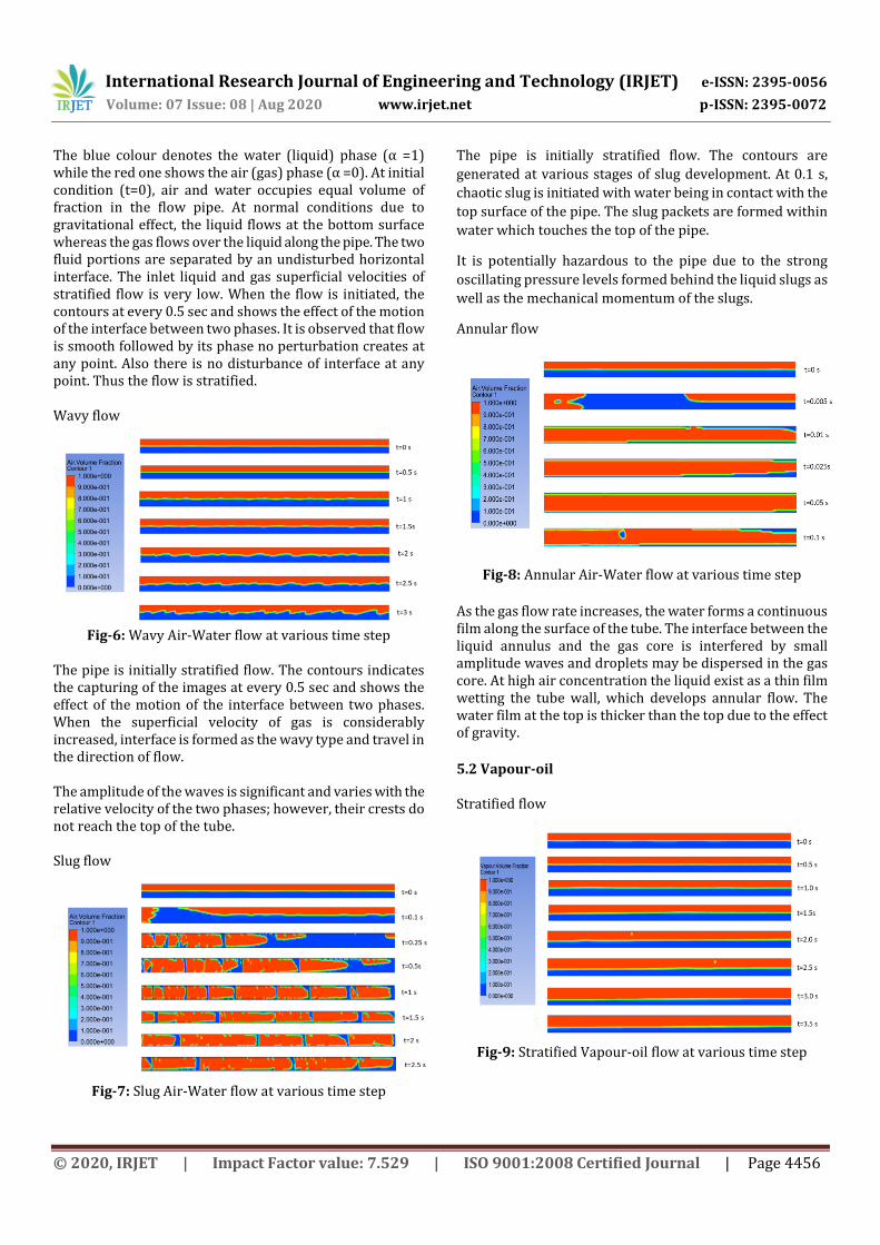
The blue colour denotes the water (liquid) phase (α =1) while the red one shows the air (gas) phase (α =0). At initial condition (t=0), air and water occupies equal volume of fraction in the flow pipe. At normal conditions due to gravitational effect, the liquid flows at the bottom surface whereas the gas flows over the liquid along the pipe. The two fluid portions are separated by an undisturbed horizontal interface. The inlet liquid and gas superficial velocities of stratified flow is very low. When the flow is initiated, the contours at every 0.5 sec and shows the effect of the motion of the interface between two phases. It is observed that flow is smooth followed by its phase no perturbation creates at any point. Also there is no disturbance of interface at any point. Thus the flow is stratified. Wavy flow

Fig-6: Wavy Air-Water flow at various time step

The pipe is initially stratified flow. The contours indicates the capturing of the images at every 0.5 sec and shows the effect of the motion of the interface between two phases. When the superficial velocity of gas is considerably increased, interface is formed as the wavy type and travel in the direction of flow. The amplitude of the waves is significant and varies with the relative velocity of the two phases; however, their crests do not reach the top of the tube. Slug flow

Fig-7: Slug Air-Water flow at various time step

The pipe is initially stratified flow. The contours are

generated at various stages of slug development. At 0.1 s,

chaotic slug is initiated with water being in contact with the

top surface of the pipe. The slug packets are formed within

water which touches the top of the pipe.

It is potentially hazardous to the pipe due to the strong

oscillating pressure levels formed behind the liquid slugs as

well as the mechanical momentum of the slugs.

Annular flow

Fig-8: Annular Air-Water flow at various time step

As the gas flow rate increases, the water forms a continuous film along the surface of the tube. The interface between the liquid annulus and the gas core is interfered by small amplitude waves and droplets may be dispersed in the gas core. At high air concentration the liquid exist as a thin film wetting the tube wall, which develops annular flow. The water film at the top is thicker than the top due to the effect of gravity.

5.2 Vapour-oil Stratified flow

Fig-9: Stratified Vapour-oil flow at various time step




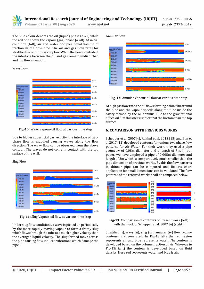
The blue colour denotes the oil (liquid) phase (α =1) while the red one shows the vapour (gas) phase (α =0). At initial condition (t=0), air and water occupies equal volume of fraction in the flow pipe. The oil and gas flow rates for stratified is condition is very low. When the flow is initiated, the interface between the oil and gas remain undisturbed and the flow is smooth. Wavy flow

Fig-10: Wavy Vapour-oil flow at various time step

Due to higher superficial gas velocity, the interface of two-phase flow is muddled causing waves along the flow direction. The wavy flow can be observed from the above contour. The waves do not come in contact with the top surface of the wall. Slug Flow

Fig-11: Slug Vapour-oil flow at various time step

Under slug flow conditions, a wave is picked up periodically by the more rapidly moving vapour to form a frothy slug which flows through the tube at a much higher velocity than the averaged liquid velocity. The slug formed move across the pipe causing flow induced vibrations which damage the pipe.

Annular flow

Fig-12: Annular Vapour-oil flow at various time step At high gas flow rate, the oil flows forming a thin film around the pipe and the vapour speeds along the tube inside the cavity formed by the oil annulus. Due to the gravitational effect, oil film thickness is thicker at the bottom than the top surface.

6. COMPARISON WITH PREVIOUS WORKS Schepper et al. 2007[4], Rahimi et al. 2013 [15] and Ban et al.2017 [12] developed contours for various two phase flow patterns for Air-Water. For their work, they used a pipe geometry of 0.08m diameter and a length of 7m. In our paper, we have employed a pipe of 0.008m diameter and length of 2m which is comparatively much smaller than the pipe dimension of previous works. By this the flow patterns in thinner pipe can be compared and Baker’s chart application for small dimensions can be validated. The flow patterns of the referred works shall be compared below.

Fig-13: Comparison of contours of Present work (left) with the work of Schepper et al. 2007 [4] (right).

Stratified (i), wavy (ii), slug (iii), annular (iv) flow regime contours are generated. In Fig-13(left) the red region represents air and blue represents water. The contour is developed based on the volume fraction of air. Whereas in Fig-13(right) the contour is developed based on fluid density. Here red represents water and blue is air.




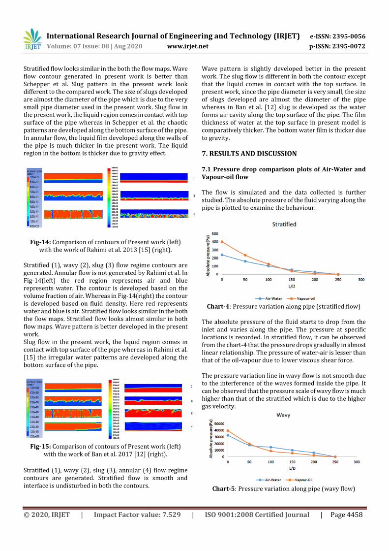
Stratified flow looks similar in the both the flow maps. Wave flow contour generated in present work is better than Schepper et al. Slug pattern in the present work look different to the compared work. The size of slugs developed are almost the diameter of the pipe which is due to the very small pipe diameter used in the present work. Slug flow in the present work, the liquid region comes in contact with top surface of the pipe whereas in Schepper et al. the chaotic patterns are developed along the bottom surface of the pipe. In annular flow, the liquid film developed along the walls of the pipe is much thicker in the present work. The liquid region in the bottom is thicker due to gravity effect.

Fig-14: Comparison of contours of Present work (left) with the work of Rahimi et al. 2013 [15] (right).

Stratified (1), wavy (2), slug (3) flow regime contours are generated. Annular flow is not generated by Rahimi et al. In Fig-14(left) the red region represents air and blue represents water. The contour is developed based on the volume fraction of air. Whereas in Fig-14(right) the contour is developed based on fluid density. Here red represents water and blue is air. Stratified flow looks similar in the both the flow maps. Stratified flow looks almost similar in both flow maps. Wave pattern is better developed in the present work. Slug flow in the present work, the liquid region comes in contact with top surface of the pipe whereas in Rahimi et al. [15] the irregular water patterns are developed along the bottom surface of the pipe.

Fig-15: Comparison of contours of Present work (left)

with the work of Ban et al. 2017 [12] (right). Stratified (1), wavy (2), slug (3), annular (4) flow regime contours are generated. Stratified flow is smooth and interface is undisturbed in both the contours.

Wave pattern is slightly developed better in the present work. The slug flow is different in both the contour except that the liquid comes in contact with the top surface. In present work, since the pipe diameter is very small, the size of slugs developed are almost the diameter of the pipe whereas in Ban et al. [12] slug is developed as the water forms air cavity along the top surface of the pipe. The film thickness of water at the top surface in present model is comparatively thicker. The bottom water film is thicker due to gravity.

7. RESULTS AND DISCUSSION 7.1 Pressure drop comparison plots of Air-Water and Vapour-oil flow The flow is simulated and the data collected is further studied. The absolute pressure of the fluid varying along the pipe is plotted to examine the behaviour.

Chart-4: Pressure variation along pipe (stratified flow)

The absolute pressure of the fluid starts to drop from the inlet and varies along the pipe. The pressure at specific locations is recorded. In stratified flow, it can be observed from the chart-4 that the pressure drops gradually in almost linear relationship. The pressure of water-air is lesser than that of the oil-vapour due to lower viscous shear force. The pressure variation line in wavy flow is not smooth due to the interference of the waves formed inside the pipe. It can be observed that the pressure scale of wavy flow is much higher than that of the stratified which is due to the higher gas velocity.

Chart-5: Pressure variation along pipe (wavy flow)




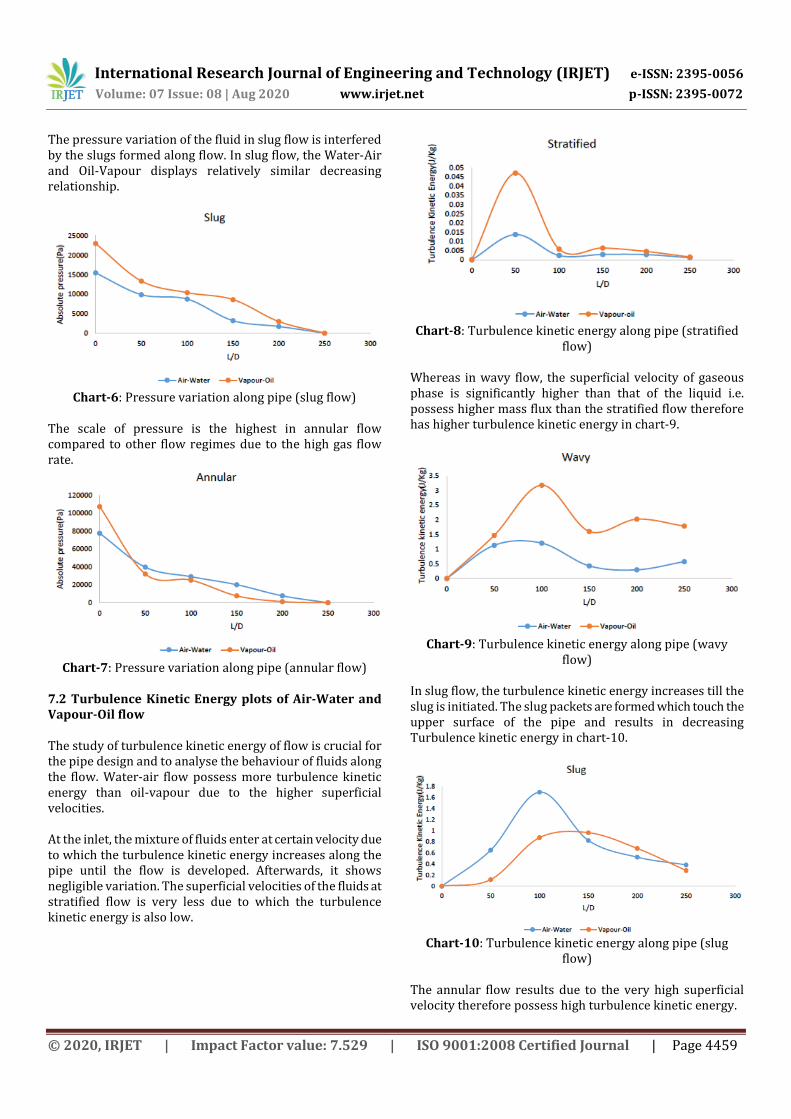
The pressure variation of the fluid in slug flow is interfered by the slugs formed along flow. In slug flow, the Water-Air and Oil-Vapour displays relatively similar decreasing relationship.

Chart-6: Pressure variation along pipe (slug flow)

The scale of pressure is the highest in annular flow compared to other flow regimes due to the high gas flow rate.

Chart-7: Pressure variation along pipe (annular flow)

7.2 Turbulence Kinetic Energy plots of Air-Water and Vapour-Oil flow The study of turbulence kinetic energy of flow is crucial for the pipe design and to analyse the behaviour of fluids along the flow. Water-air flow possess more turbulence kinetic energy than oil-vapour due to the higher superficial velocities. At the inlet, the mixture of fluids enter at certain velocity due to which the turbulence kinetic energy increases along the pipe until the flow is developed. Afterwards, it shows negligible variation. The superficial velocities of the fluids at stratified flow is very less due to which the turbulence kinetic energy is also low.

Chart-8: Turbulence kinetic energy along pipe (stratified

flow) Whereas in wavy flow, the superficial velocity of gaseous phase is significantly higher than that of the liquid i.e. possess higher mass flux than the stratified flow therefore has higher turbulence kinetic energy in chart-9.

Chart-9: Turbulence kinetic energy along pipe (wavy

flow) In slug flow, the turbulence kinetic energy increases till the slug is initiated. The slug packets are formed which touch the upper surface of the pipe and results in decreasing Turbulence kinetic energy in chart-10.

Chart-10: Turbulence kinetic energy along pipe (slug

flow) The annular flow results due to the very high superficial velocity therefore possess high turbulence kinetic energy.




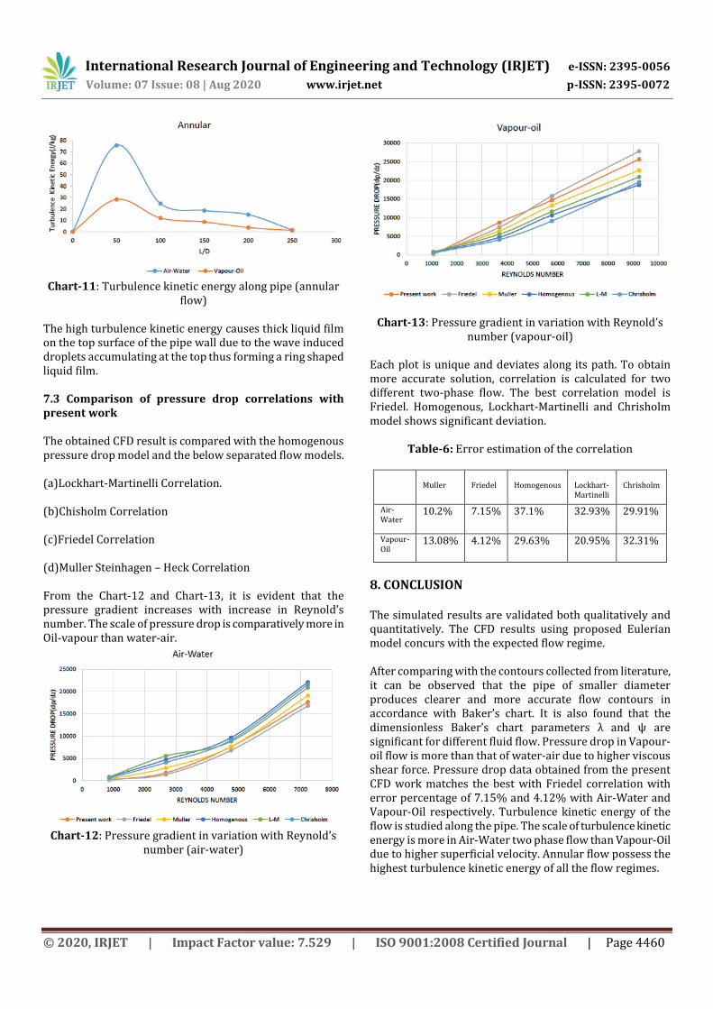
Chart-11: Turbulence kinetic energy along pipe (annular

flow) The high turbulence kinetic energy causes thick liquid film on the top surface of the pipe wall due to the wave induced droplets accumulating at the top thus forming a ring shaped liquid film. 7.3 Comparison of pressure drop correlations with present work The obtained CFD result is compared with the homogenous pressure drop model and the below separated flow models. (a)Lockhart-Martinelli Correlation. (b)Chisholm Correlation (c)Friedel Correlation (d)Muller Steinhagen – Heck Correlation From the Chart-12 and Chart-13, it is evident that the pressure gradient increases with increase in Reynold’s number. The scale of pressure drop is comparatively more in Oil-vapour than water-air.

Chart-12: Pressure gradient in variation with Reynold’s

number (air-water)

Chart-13: Pressure gradient in variation with Reynold’s number (vapour-oil)

Each plot is unique and deviates along its path. To obtain more accurate solution, correlation is calculated for two different two-phase flow. The best correlation model is Friedel. Homogenous, Lockhart-Martinelli and Chrisholm model shows significant deviation.

Table-6: Error estimation of the correlation

Muller

Friedel

Homogenous

Lockhart-Martinelli

Chrisholm

Air-Water

10.2% 7.15% 37.1% 32.93% 29.91%

Vapour-Oil

13.08% 4.12% 29.63% 20.95% 32.31%

8. CONCLUSION The simulated results are validated both qualitatively and quantitatively. The CFD results using proposed Eulerian model concurs with the expected flow regime. After comparing with the contours collected from literature, it can be observed that the pipe of smaller diameter produces clearer and more accurate flow contours in accordance with Baker’s chart. It is also found that the dimensionless Baker’s chart parameters λ and ψ are significant for different fluid flow. Pressure drop in Vapour-oil flow is more than that of water-air due to higher viscous shear force. Pressure drop data obtained from the present CFD work matches the best with Friedel correlation with error percentage of 7.15% and 4.12% with Air-Water and Vapour-Oil respectively. Turbulence kinetic energy of the flow is studied along the pipe. The scale of turbulence kinetic energy is more in Air-Water two phase flow than Vapour-Oil due to higher superficial velocity. Annular flow possess the highest turbulence kinetic energy of all the flow regimes.




ACKNOWLEDGEMENT The members of the group would like to acknowledge all those who helped with the completion of this project. We would like to thank the faculty in charge Prof. Padmanathan P for helping us choose the topic and monitoring our progress right from the beginning to the end. He has provided us valuable knowledge and advice. We should thank the authors of the reference papers for their inputs. We would also like to thank the School of Mechanical Engineering (SMEC), Vellore Institute of Technology for providing us the facilities to complete the project.

REFERENCES [1] Esteban Guerrero, Felipe Muñoz and Nicolás Ratkovich,

2017. Comparison between eulerian and VOF models for two-phase flow assessment in vertical pipes. Journal of oil, gas and alternative energy sources.

[2] C Rajesh Babu, 2013. CFD Analysis of Multi-Phase Flow And Its Measurements. IOSR Journal of Mechanical and Civil Engineering.

[3] Swanand M. Bhagwat, Afshin, J. Ghajar, 2013. A flow pattern independent drift flux model based void fraction correlation for a wide range of gas–liquid two phase flow. International Journal of Multiphase Flow.

[4] Sandra C.K. De Schepper, Geraldine J. Heynderickx, Guy B. Marin, 2007. CFD modelling of all gas–liquid and vapour–liquid flow regimes predicted by the Baker chart. Chemical Engineering Journal - 138.

[5] P. Bhramara, V. D. Rao, K. V. Sharma, and T. K. K. Reddy, 2008. CFD Analysis of two-phase flow in a horizontal pipe- prediction of pressure drop.

[6] Archibong Archibong-Eso & Jing Shi & Yahaya D. Baba, 2018. High viscous oil–water two–phase flow: experiments & numerical simulations. Heat and Mass Transfer.

[7] Bryan T. Cacho, 2011. CFD Analysis of Two-Phase Flow Characteristics in a 90 Degree Elbow. United Nations University, Geothermal Training program 2015.

[8] H. Pineda-Perez, T. Kim, E. Pereyra, N. Ratkovich, 2018. CFD modelling of air and highly viscous liquid two-phase slug flow in horizontal pipes. Chemical Engineering Research and Design.

[9] Quamrul H. Mazumder and Saiful A. Siddique, 2011. CFD Analysis of Two-Phase Flow Characteristics in a 90 Degree Elbow. Journal of Computational Multiphase Flows.

[10] Milad Darzi, Chanwoo Park, 2017. Experimental visualization and numerical simulation of liquid-gas two-phase flows in a horizontal pipe. ASME 2017 International Mechanical Engineering Congress and Exposition.

[11] V.Jagan, A Satheesh, 2016. Experimental studies on two phase flow patterns of air-water mixture in a pipe with different orientations. Flow Measurement and Instrumentation.

[12] Sam Ban, William Pao and Mohammad Shakir Nasif, 2017. Numerical simulation of twophase flow regime in horizontal pipeline and its validation. Emerald Insight.

[13] Hai-fei Liu, Jing-yu Xu, Ying-xiang Wu , Zhi-chu Zheng, 2015. Numerical study on oil and water two-phase flow in a cylindrical cyclone. ScienceDirect 9th International Conference on Hydrodynamics.

[14] Satheesh A, 2014. Computational analysis of two-phase flow distribution in a horizontal pipe. Applied Mechanics and Materials.

[15] Rahimi, R., Bahramifar, E. and Sotoodeh, M.M. (2013), “The indication of two-phase flow pattern and slug characteristics in a pipeline using CFD method”, Gas Processing Journal, Vol. 1 No. 1, pp. 70-87.

Documents

Computational Analysis of Two-Phase flow in Horizontal