Embed Size (px)
Citation preview

Model-based estimation of multi-phase flows in horizontal wells


Model-based estimation of multi-phase flows in horizontal wells
PROEFSCHRIFT
ter verkrijging van de graad van doctor aan de Technische Universiteit Delft,
op gezag van de Rector Magnificus prof. ir. K.C.A.M. Luyben, voorzitter van het College voor Promoties,
in het openbaar te verdedigen op maandag 21 februari 2011 om 10:00 uur
door
Anton Nikolaevich GRYZLOV
Hydraulic engineer, Moscow State Technical University, Russia
geboren te Moskou, Sovjet-Unie

Dit proefschrift is goedgekeurd door de promotor: Prof. dr. R.F. Mudde Samenstelling promotiecommissie: Rector Magnificus, voorzitter Prof. dr. R.F. Mudde, Technische Universiteit Delft, promotor Prof. dr. ir. R.A.W.M. Henkes, Technische Universiteit Delft Prof. dr. B.J. Azzopardi, University of Nottingham, UK Prof. dr. S.M. Luthi, Technische Universiteit Delft Prof. dr. ir. P.M.J. Van den Hof, Technische Universiteit Delft Prof. dr. ir. H.W.M. Hoeijmakers, Universiteit Twente Dr. R. van der Linden, TNO Industrie en Techniek Prof. dr. ir. H.E.A. van den Akker, Technische Universiteit Delft, reservelid This research was carried out within the context of the ISAPP Knowledge Centre. ISAPP (Integrated Systems Approach to Petroleum Production) is a joint project of the Netherlands Organization for Applied Scientific Research TNO, Shell International Exploration and Production, and Delft University of Technology ISBN: 978-90-6464-455-9 Keywords: wellbore flow, inverse dynamic problem, multiphase flow metering Printed by: GVO drukkers & vormgevers B.V. I Ponsen & Looien Cover design by: Tanya Kudryashova © 2011 A. Gryzlov All rights reserved. No part of the material protected by this copyright notice may be reproduced or utilized in any form or by any means, electronic or mechanical, including photocopying, recording or by any information storage and retrieval system, without written permission from the author.

v
Contents SAMENVATTING .............................................................................................................. 1
SUMMARY.......................................................................................................................... 3
1. INTRODUCTION ........................................................................................................... 5
1.1. MULTIPHASE FLOW METERING.................................................................................... 5 1.2. MULTIPHASE FLOWS ................................................................................................. 15 1.3. SMART WELLS AND SOFT-SENSING .......................................................................... 23 1.4. DISCUSSION AND RESEARCH DIRECTIONS ................................................................ 31 1.5. OUTLINE ................................................................................................................... 33
2. WELLBORE FLOW MODEL..................................................................................... 35
2.1. GOVERNING EQUATIONS FOR A DRIFT-FLUX MODEL ................................................. 35 2.2. ALGEBRAIC SLIP MODEL .......................................................................................... 39 2.3. MATRIX FORM OF CONSERVATION EQUATIONS ......................................................... 42 2.4. SUMMARY................................................................................................................. 47
3. NUMERICAL METHODS........................................................................................... 49
3.1. INTRODUCTION ......................................................................................................... 49 3.2. DISCRETIZATION OF THE FLOW EQUATIONS .............................................................. 52 3.3. NUMERICAL EXAMPLE. NEED FOR SOURCE TERM CORRECTION ................................ 59 3.4. NUMERICAL EXAMPLES............................................................................................. 66 3.5. SUMMARY................................................................................................................. 73
4. A SEMI-IMPLICIT EXTENDED KALMAN FILTER............................................. 75
4.1. INTRODUCTION ......................................................................................................... 75 4.2. FORMULATION OF THE INVERSE PROBLEM ................................................................ 77 4.3. STATE-SPACE FORM OF MODEL EQUATIONS .............................................................. 79 4.4. DATA ASSIMILATION CONCEPTS................................................................................ 80 4.5. RESULTS AND DISCUSSIONS ...................................................................................... 83 4.6. SUMMARY AND CONCLUSIONS .................................................................................. 89
5. INVERSE MODELLING OF THE INFLOW DISTRIBUTION FOR THE LIQUID/GAS FLOW IN HORIZONTAL PIPELINES ................................................ 91
5.1. INTRODUCTION ......................................................................................................... 91 5.2. QUALITATIVE ANALYSIS OF PRESSURE TRANSIENTS.................................................. 93 5.3. FORMULATION OF THE INVERSE PROBLEM ................................................................ 98 5.4. RESULTS AND DISCUSSIONS .................................................................................... 102 5.5. CONCLUSIONS......................................................................................................... 113
6. ESTIMATION OF THE MULTIPHASE INFLOW FOR GAS BREAKTHROUGH CONTROL....................................................................................................................... 115
6.1. INTRODUCTION ....................................................................................................... 115 6.2. FORMULATION OF THE ESTIMATION PROBLEM ........................................................ 118 6.3. RESULTS AND DISCUSSIONS .................................................................................... 121

vi
6.4. CONCLUSIONS......................................................................................................... 131
7. CONCLUSIONS AND FUTURE WORK ................................................................. 133
7.1. MODELLING AND SIMULATIONS.............................................................................. 133 7.2. DATA ASSIMILATION .............................................................................................. 134 7.3. SOFT-SENSING ........................................................................................................ 135 7.4. SUGGESTIONS FOR FUTURE WORK.......................................................................... 137
BIBLIOGRAPHY............................................................................................................ 139
APPENDIX A. DERIVATION OF THE FULLY EXPLICIT PARAMETER ESTIMATOR................................................................................................................... 147
APPENDIX B. EXPERIMENTAL SETUP DESIGN .................................................. 151
AFTERWORD................................................................................................................. 155
ABOUT THE AUTHOR ................................................................................................. 157

Samenvatting _________________________________________________________________________
1
Samenvatting The groeiende vraag naar koolwaterstofproducten heeft geresulteerd in een verbeterd management van olievelden met verscheidene regel- en optimalisatiestrategien. Deze strategieën vertrouwen sterk op de efficiency van ondergrondse apparatuur die gebruikt wordt voor het verkrijgen van real-time olie- and gasproductiesnelheidsmetingen met voldoende resolutie in plaats en tijd. Ondergronds geïnstalleerde meerfasestromingsmeters in het bijzonder kunnen the productie van horizontale putten verbeteren door het identificeren van de zones waar olie, gas en water instroomt. Bestaande meerfasestromingsmeters zijn echter duur, onnauwkeurig of alleen nauwkeurig binnen een beperkt werkgebied en daarom is een dergelijke manier van monitoren onrealistisch. Om deze problemen te overwinnen kan men gebruikmaken van zogenaamde meerfasen soft(ware)sensoren, waarmee productiesnelheden worden afgeschat met conventionele meetapparatuur zoals drukmeters in combinatie met een dynamisch meerfasestromingsmodel. De soft-sensoren kunnen ook worden gebruikt in combinatie met hardware sensoren om hun prestaties te verbeteren, bijvoorbeeld door het vervangen van weggevallen data met outputs van de soft-sensor. Via een dergelijke constructie kunnen ze ook gebruikt worden voor het diagnosticeren van afwijkende situaties of een defect van een hardware sensor. Het onderzoek dat gepresenteerd wordt in deze thesis bediscussieert mogelijkheden en beperkingen van dergelijke meerfasenstromings-softsensoren. Allereerst wordt er een numeriek model ontwikkeld voor het voorspellen van snelle overgangen in gas-vloeistofstromingen. Een drift-flux benadering wordt daartoe gebruikt die één-dimensionale gas-vloeistofstromingen in een horizontaal boorgat beschrijft. Het resulterende drift-flux model bestaat uit een continuiteitsvergelijking voor elke fase en een impulsvergelijking voor de gehele vloeistof-gasmengsel. Het verschil tussen vloeistof- en gassnelheden wordt verdisconteerd door het gebruik van een algebraïsche slipvergelijking. De numerieke oplossing wordt verkregen door gebruik te maken van een expliciet flux-splitting schema. Een speciale behandeling van de brontermen, die de instroming vanuit het reservoir karakteriseren, is vereist om de conservatieve eigenschappen van het schema te behouden. Dit wordt bewerkstelligd door het uitbreiden van de schema’s die zijn ontwikkeld voor niet-homogene hyperbolische vergelijkingen, waar als noviteit een geïntegreerde bron is geïntroduceerd die een exacte balans behoudt met fluxgradiënten. De resulterende nieuwe boorgatsimulator is getest aan de hand van een serie van generieke testcases, waarbij de verkregen simulatieresultaten zijn vergeleken met data gegenereerd door de commercieel verkrijgbare boorgatsimulator OLGA. De verkregen resultaten tonen aan dat de nieuwe simulator nauwkeurige voorspellingen van stromingsvariabelen genereert. In een volgende stap is de invloed bestudeerd van het tijdsintegratieschema op de

Samenvatting _________________________________________________________________________
2
resultaten van data assimilatie gebaseerd op het Extended Kalman Filter. Het gebruik van het impliciete Eulerschema, dat onvoorwaardelijk stabiel is over het gehele gebied van tijdstappen voor zowel de update van het model als voor de update van de covariantie, resulteert in minder nauwkeurige schattingen. Dit kan worden voorkomen door gebruik te maken van een parameterschatter gebaseerd op het expliciete Eulerschema. Dit schema beperkt echter in hoge mate de maximale tijdstap die kan worden gebruikt voor de tijdsintegratie, wat leidt tot te lange simulatietijden. Een alternatieve oplossing is gevonden in het gebruik van een semi-impliciete schatter waarbij het model up-to-date wordt gebracht met het impliciete Eulerschema terwijl de tijdspropagatie van de fout-covariantiematrix gebaseerd is op het expliciete Eulerschema. Deze hybride benadering combineert de nauwkeurigheid van het conventionele Kalman Filter met de robuustheid van het impliciete voorwaarts modelleren. Het voorgestelde algoritme is succesvol toegepast op het een-dimensionale probleem van het schatten van permeabiliteit in een poreus medium voor een enkelfase oliestroming. Tenslotte wordt een nieuwe benadering gepresenteerd voor de optimale regeling en real-time monitoring van horizontale putten. Deze methodologie gebruikt inverse modelconcepten voor het schatten van ondergrondse stromingssnelheden die niet direct worden gemeten. De analyse van een dynamische drukresponsie op een snelle instroming vanuit het reservoir heeft aangetoond dat de beschikbare informatie niet voldoende is voor het simultaan schatten van snelheids- en samenstellingscomponenten omdat deze op verschillende tijdsschalen acteren. De voorgestelde real-time schatter gebruikt een dynamisch model van de meerfasenpijpstroming en informatie van conventionele ondergrondse sensoren. De prestatie van het voorgestelde algoritme is bestudeerd met op simulatie gebaseerde studies voor zowel ruisverstoorde synthetische metingen als kunstmatige data gegenereerd door de OLGA simulator. De verkregen resultaten duiden erop dat de voorgestelde model gebaseerde schatter veelbelovend is voor real-time productieoptimalisatie doeleinden.

Summary _________________________________________________________________________
3
Summary The growing demand for hydrocarbon production has resulted into improved oilfield management with various control and optimization strategies. These strategies in turn strongly rely on the efficiency of downhole equipment which is used to obtain real-time oil and gas production rates with sufficient spatial and temporal resolution. In particular, multiphase flowmeters installed downhole can improve the production of horizontal wells by allocating the zones of oil, gas and water inflow. However, existing multiphase meters are expensive, inaccurate or accurate only within a limited operating range and therefore such monitoring is unrealistic. To overcome these problems one can use so-called multiphase soft-sensors, i.e. to estimate flow rates from conventional meters, such as downhole pressure gauges, in combination with a dynamic multiphase flow model. The soft-sensors can also be used together with hardware sensors to improve their overall performance, e.g. by substituting missing data of the hardware sensor with output of the soft-senor. The research presented in this thesis discusses possibilities and limitations of such multiphase soft-sensors. First a numerical model has been developed and used to predict rapid transients in gas-liquid flows. A drift-flux model which describes one-dimensional gas-liquid flows in a horizontal wellbore is considered in this work. This model consists of a continuity equation for each phase and a momentum equation written for the mixture. The difference between liquid and gas velocities is taken into account using an algebraic slip relation. The numerical solution is obtained using an explicit flux-splitting scheme. A special treatment of the source terms, which characterize an inflow from the reservoir, is required in order to preserve the conservative properties of the scheme. This is achieved extending the schemes developed for non-homogeneous hyperbolic equations, where an integrated source is newly introduced, which retains an exact balance with flux gradients. This new wellbore simulator has been tested on a series of generic test cases, comparing it to data generated by OLGA, a commercially available wellbore simulator. The obtained results show that the new simulator provides accurate predictions of flow variables. An assessment of the time-integration scheme impact on results of data assimilation based on the extended Kalman filter approach is performed. The use of the implicit Euler scheme, which is unconditionally stable for the whole range of time steps both for the model and covariance update, results in a less accurate estimates, which can be overcome using a parameter estimator based on the explicit Euler scheme. However, the latter strongly limits the maximum time step, which can be used, and leads to inappropriate simulation time. An alternative can be found using a semi-implicit estimator, where a model is updated using the implicit Euler scheme, whereas the propagation of the error covariance matrix in time is based on the explicit time integration scheme. This hybrid

Summary _________________________________________________________________________ 4
approach combines the accuracy of the conventional Kalman filtering with the robustness of the implicit forward modelling. The proposed algorithm is successfully applied for the solution of the one-dimensional problem of permeability estimation in a porous medium for a single phase oil flow. Finally, a new approach for optimal control and real-time monitoring of horizontal wells is presented. This methodology uses inverse modelling concepts to estimate downhole flow rates that are not measured directly. The analysis of transient pressure response due to a rapid inflow from a reservoir has shown that the available information is not sufficient to estimate simultaneously velocity and composition components, as they act on the different time scales. The real-time estimator proposed uses a dynamic model of the multiphase pipe flow and information from conventional downhole sensors. The performance of the proposed algorithm has been studied for simulation based case studies both for noisy synthetic measurements and artificial data generated by the OLGA simulator. The obtained results indicate that the model based estimator proposed is promising for real-time production optimization purposes.

Chapter 1. Introduction _________________________________________________________________________
5
1. Introduction
1.1. Multiphase flow metering
A multiphase flow meter is a device for measuring the individual liquid and gas rates in a multiphase flow. In the petroleum engineering nomenclature multiphase refers to a flow which consists of some or all of the following phases: a liquid hydrocarbon phase (crude oil or gas condensate), a gas phase (natural gas or air), a water phase and a solid phase. Multiphase flow meters (MPFM) measure oil, gas and water production rates in situ, i.e. without separating the flow components. In contrast, conventional metering of the multiphase flow is carried out using two or three phase test separators (full or partial separation) that segregate and measure gas, oil and water flowrates at surface processing facilities [Williams, 1994]. Obtaining accurate measurements from a test separator requires relatively stable conditions within the device. A long period of steady operation may be required to achieve such conditions, which is inconvenient in a production facility. Moreover, harsh operating regimes may prevent a complete separation of phases involved: as a result of changing operating conditions, gas may flash out of oil or be absorbed by the liquid; waxes and hydrate precipitations may occur. Test separators also have difficulty measuring certain flow patterns, characterized by unstable or rapidly changing conditions. Such problematic flow regimes include slug flow, which is characterized by the discrete liquid slugs followed by gas bubbles with correspondingly large variations in water cuts and changes in fluid properties. In contrast, multiphase flowmeters perform direct measurements on an unseparated multiphase flow in a pipeline. Information on flowrates is available to the user within minutes after starting the operation. Although the traditional method of separating the phases before measuring is still used for the fiscal metering [Theuveny et al., 2002], MPFM systems are now increasingly employed in various hydrocarbon production systems where accuracy requirements are less stringent. MPFM systems can be used for continuous production monitoring since they yield flow rates continuously at a high sampling frequency, which is not practical using a test separator. Furthermore, production monitoring implies the ability to track, in real time, any changes in fluid composition, flow rates, pressure and temperature. Combining such information with historical data and static or dynamic flow models describing the physics of a production system helps to diagnose current problems and predict its future performance [Retnando et al., 2001]. Multiphase flowmeters installed downhole can improve the production of long horizontal wells producing oil, gas and water inflow from several production intervals. Downhole MPFM are best suited for “intelligent wells”, where

Chapter 1. Introduction _________________________________________________________________________ 6
permanent monitoring and control is used to optimize production [Glandt, 2003]. Combined with adjustable inflow control devices, the flow distribution between the various sections can be optimized, for example by detecting and preventing gas coning or water breakthrough from specific producing sections [Leemhuis et al., 2008]. Such systems installed downhole provide real-time information on variations in gas and liquid flow rates, so that well slugging effects or other production instabilities may be detected as they occur. A further application of downhole flowmeters is in production from multi-lateral wells. Since monitoring the flow at the surface provides no information about multiphase flow in individual branches, downhole metering systems can be a valuable diagnostic tool, as they provide continuous real-time data on individual flow contributions. For the subsea commingled long flow lines MPFM systems may be used for monitoring of flow rates from individual wells or pipelines [Kragas et al., 2003]. In addition, it will eliminate the need of a surface test separator, which significantly reduces the footprint requirement on offshore platforms. It should be noted, however, that retrieving a MPFM for maintenance or repair may be problematic or even impossible once it has been installed downhole. Recalibrating the meter may be difficult and verification methods are required to ensure correct flowmeter operation. The ability of a MPFM to respond quickly to any change in fluid composition and the reduced time to stabilize the flow may be used for production optimization purposes [Kettle and Ross, 2002]. For wells which are assisted by the gas lift technique, production is maximized for a certain optimum amount of injection gas. The optimization of gas lift requires detailed knowledge of the flow rates, bottom-hole pressure and water cut, which are usually obtained via a test separator by performing a multi-rate test. Since the result of this test may vary with changes of bottom-hole pressure and water cut the optimum gas lift performance point will be drifting, requiring additional testing of such wells. MPFM can help to find the optimal gas lift injection rate, and provide relevant data on a continuous basis for performing optimization [Aspelund et al., 1996]. In a conventional flow measurement an extra test separator dedicated for well test or other purposes is used. The flowrates are measured by separating one well stream and directing it all the time to the test-separator. Multiphase metering performed with test separators requires regular intervention of qualified personnel and cannot provide continuous well-monitoring. If MPFM is able to perform measurements in the absence of a flow reference it could be used instead of the test separator as permanently installed device on each well or be installed in addition to an existing test separator. Such configuration is also preferable if it is necessary to monitor simultaneously one well and test another. The main advantage of the MPFM over the test separator is the reduction in time to perform a measurement and elimination of test lines, valves, manifolds and even slug catchers.

Chapter 1. Introduction _________________________________________________________________________
7
Basic Principles The primary output information of any MPFM system consists of the mass flow rates of oil, water and gas components in the flow. Ideally, a flow meter will provide a user with the direct measurements of the phase rates. Unfortunately, for a three-phase flow there is no single measurement principle, which yields all these flowrates independently and it is necessary to integrate several different measuring instruments in one tool and to obtain the flow rates by combining the output of those primary sensors [Ribeiro, 1996; Falcone et al., 2002; Thorn et al., 1997]. Although there are many possible solutions as well as a number of potential instruments to be used, this indirect method usually measures the average fluid velocity and cross-sectional fraction of each phase (liquid holdup or void fraction). Using these quantities, supplemented with knowledge of densities of the fluids, one can calculate phase and total flow rates. To determine mass flow rates in a three phase flow, three measurements of oil, water and gas velocities and two volume fractions are required. Furthermore, the densities of the different phases must be known. It should be noted here that it may not be necessary to measure all these properties explicitly if information can be inferred from specific flow characteristics. However, in the latter case the correlation between measured parameters and the flow rates of the respective phases must be established. Such relationships may not exist, or may not be universal over the full range of operating conditions. Two strategies can be used to reduce the number of required measurements: separation and homogenization [Hewitt et al., 1995; Hanssen and Torklidsen, 1995]. Full separation of a three phase flow removes the need of measuring volume fractions and mass flow rates are measured using conventional single-phase metering techniques. Where a complete separation for multiphase metering applications can still be expensive or even not feasible, systems based on partial separation are used [Schook and van Asperen, 2005] are used. For these purposes compact inline separation technology is employed [Hamoud et al., 2008], which utilizes the centrifugal force to divide the flow into the liquid phase and a gas phase. Separation may not be complete in such systems, but acceptable measurement accuracy can be achieved in a narrow range of flow conditions. Homogenization involves mixing the flow to ensure all phase velocities are identical. Only this single velocity and two volume fractions are required to derive phase mass flow rates. It can be difficult to obtain a homogeneous mixture since water does not mix well with oil, and gas tends to separate from liquids. This in turn may cause unpredictable results in calculating the properties of the obtained mixture (density, viscosity). Even if the components are well-mixed, there can be a substantial slip between heavy and light phases, which will make a single velocity assumption inapplicable. The typical example of an MPFM, based on a homogenization principle, is a Venturi-based meter (Figure 1.1).

Chapter 1. Introduction _________________________________________________________________________ 8
The total mass flow rate is calculated using the measured pressure drop p over
the Venturi throat. The pressure drop between the entry and throat can be roughly approximated by Bernoulli’s equation. If all the three-phases are mixed well and the velocities of the phases are equal, the flow velocity at the throat is given by
2
th
m
pu C
(1.1)
where C is a Venturi coefficient and m is the mixture density. Mixture density can be measured using a attenuation method, which is based on
the principle that a more dense material attenuates gamma rays more strongly than a lighter one.
p
source
detector
Figure 1.1. Scheme of Venturi multiphase flow meter (after Atkinson et al., 2000)
For the meter configuration given in Figure 1.1., a source of gamma radiation with intensity of I0 is placed on one side of the Venturi throat with a detector placed on the opposite side. The intensity of a monochromatic beam which has passed through the oil-gas-water mixture is given by [Petrick and Swanson, 1958]:
0 0exp( ( (1 ) ))o w w o w gI I d (1.2)
Here o, w, g are the linear attenuation coefficients of oil, water and gas phases,
respectively, d is the diameter of the measuring section. In order to determine the oil and
water volume fractions wusing this technique two independent measurements are
required, which can be obtained using two radiation sources with different attenuation coefficients. This dual-energy technique [Roach et al., 1994] provides both mixture density and phase density information. Although gamma ray methods can be used over the complete range of holdups, the salinity of water phase can cause problems. Since salt has a

Chapter 1. Introduction _________________________________________________________________________
9
high attenuation coefficient compared to the one of water, a change in the salinity of the water phase will cause a significant error in the measured water fractions. The third energy level is then used to calculate the salinity of the water phase [Pinguet et al., 2006]. Despite the advantages of the Venturi-based flow meter (non-intrusiveness, no moving parts), it possesses a number of difficulties. High measurement accuracy requires more intense radiation sources, which affects safety aspects and mobility considerations. The phase fractions then will only be representative over a cross-section if the phases are homogeneously mixed. This in turn may be overcome by using multi-beam systems [Smith, 1975], though it inevitably leads to more expensive design of the meter.
Figure 1.2. Scheme of flow rate metering with Venturi meter.
At first glance one can think that the required quantities, i.e. phase fractions and velocities are obtained directly from the equipment used. However, data acquired with measurement hardware do not necessarily correspond to the information needed. For a Venturi meter this is illustrated in Figure 1.2. Any measurement system consists of three components: 1) Measurement; 2) Computation; 3) User interface. Though measurements are a very first action that is performed to extract any sensible piece of information, the computation part is generally needed either to filter obtained data, or to combine signals acquired from different parts of the measuring system,

Chapter 1. Introduction _________________________________________________________________________ 10
in order to obtain quantities relevant to a user. In a Venturi meter this is done, for example, by employing equation (1.2) which converts pressure drop (measured) into total mass flow rate (computed) via a known mathematical model (Bernoulli’s equation). Since flow rates are calculated as a combination of the different sources of information, the propagation of a measurement error in the entire algorithm will greatly influence the performance of the meter. It clearly follows from the above that the measurement error can be decreased either by improving hardware performance or by using more complex flow models. For example, equation (1.2) can be adjusted by incorporating slip between the phases [Atkinson et al., 2000]. This in turn may increase uncertainty in calculated parameters, as these models may require extensive calibration, e.g. by means of numerous experiments.
Industrial MPFM solutions With the variety of technological solutions available for multiphase flow metering, oil service companies are providing the MPFM systems for specific applications. Some of these developments are briefly discussed below. The MPFM system introduced by Schlumberger [Pinguet et al., 2006] consists of a Venturi meter equipped with differentional pressure sensors, and a dual-energy spectral gamma ray detector paired with a single, low strength radioactive chemical source. A single radioactive Barium source emits gamma rays at various energy levels – 32, 81 and 356 keV, with the dual energy spectral gamma ray detector installed opposite of it. First two energy levels correspond to mixture density and composition measurements, and the third energy level (usually 356 keV) could be used to measure salinity or any heavy component inside the flowing mixture. It has been reported [Theuveny et al., 2001] that the maximum gas volume fraction is 98%, with the relative accuracy of 3% below this limit. The three phase downhole flow meter developed by Weatherford uses fiber optic flow measurement technology, and is based on measuring unsteady pressures associated with turbulent flows and naturally occurring acoustics [Kragas et al., 2002a]. The metering principle is based on measuring the force applied on the internal surface of the pipe by the pressure fluctuations. By tracking the convective velocity of the turbulent eddies and the propagation velocity of sound waves, the flow velocity and the speed of sound of the medium are calculated. One of the main advantages of this flow meter is the absence of complex downhole electronics and moving parts and its nonradioactive principle. The robustness of the meter also allows operators to perform wellbore operations with the flow meter installed downhole. The operating temperature is about 1600C with a maximum pressure of 1000 bar. The two-phase design was successfully tested on the Nimr field [Kragas et al., 2002b], where the flowmeters were installed in two high water cut wells. Compared to results from a reference flow meter, the average differences in water cuts were less than 2%. A three-phase meter used at Mahogany field [Kragas et al., 2003] provided

Chapter 1. Introduction _________________________________________________________________________
11
gas, oil and water flow rates with accuracy better than 10%, for a gas volume fraction up to 75%. The metering solutions described above are designed to work in hostile downhole environment that imposes special restriction on the instrumentation design standards. To limit the need for complex devices downhole one can use a mathematical model of a process. Less physical measurements are then required, improving reliability and reducing operational costs. Wrobel [Wrobel et al., 2009] investigated a method to perform multiphase flow measurements in liquid-gas flows using only cheap, easily installable non-intrusive components. In the proposed device, pressure peaks generated in the flow are measured using standard accelerometers mounted on the outer surface of a pipeline. The method was mainly aimed to deal with intermittent flow which provides data with distinguishable pressure signals from which the slug frequency velocity can be derived in case of intermittent flow. In order to estimate phase flow rates from the obtained data semi-empirical models are used [Oliemans, 1998]. The flow-meter has been validated on an experimental setup owned by TU Delft with the accuracy better than 15% for all range of flow conditions considered. The applicability of this method is limited to flow regimes with periodic structure (slugs, waves), which are characterized by any distinctive signals (i.e. peaks). This is an example of indirect measurement of flow properties, and the relationship between the distinctive signal to be detected and flow or phase velocities must be determined a priori, using theory or calibration experiments.
The applicability of this method is limited to slug, stratified wavy, elongated bubble or annular wavy flow since only these flow regimes provide the necessary unsteady pressure signal. This limitation results in a narrow operating envelope compared to commercially available systems. Currently, the necessary empirical relationships linking measured properties to flow rates have only been developed for slug flow. It is not known whether this concept can be extended to a wider operating range. Gudmundsson and Falk, (1999) introduced the pressure pulse method to measure flow rates in gas-liquid flows. The method is based on the combined effects of water-hammer when a valve installed in a flow line is closed quickly and measurement of the speed of sound of the mixture of the pipeline. The measurement system consists of a remotely operated valve which is installed on the flowline upstream of the choke and two pressure transducers. By activating this valve a pressure wave is generated, which propagates in the upstream direction. The speed of sound in a gas-liquid mixture can be determined from the time it takes for the pressure pulse to travel the known distance between the pressure sensors. Using a relevant correlation for pressure acceleration and static pressure drop, and a slip relation if needed, the gas and liquid flow rates are calculated.

Chapter 1. Introduction _________________________________________________________________________ 12
Recently neural networks have been used in order to increase the accuracy of various measurement equipment, such as the conductance probe, Venturi meter and gamma attenuation methods. The main advantage of artificial networks is that they do not use predefined rules, contrary to conventional data processing techniques but rather learn from existing training data sets. However, these intelligent systems might fail to reproduce reality when working outside the range of conditions within which they were calibrated. Meribout et al., (2009) presented an ultrasonic-based device for the determination of the flow rates of the multiphase mixture without prior separation of the gas phase. The use of different type of ultra-sound sensors helps to cover all the flow regimes, including stratified flow. Some physical mechanisms are introduced in the pattern recognizing system. The latter uses a dedicated multilayer neural network algorithm to overcome the non-linearity and uncertainty of the sensors used. The experimental results indicate an error of ~10% can be achieved for the gas fractions up to 90%. A neural network approach has been applied to predict the flow rates of a three phase flow through a Venturi meter [Alimonti and Bilardo, 2001]. It has been shown that the use of artificial neural networks may lead to a better accuracy compared to one obtained with mechanistic flow models. Although the obtained results present relative errors below 10% over all range of flow conditions considered, it was still difficult to generalise this application of neural networks to different fluids and different flow conditions, which are out of scope of the network training. The multiphase flow metering solution proposed by Shell consists of using data-driven modelling [Goh et al., 2008]. Data-driven models have the potential to act as virtual flow meters, relating for example pressure and temperature changes in a wellbore to well production rates. Such an approach provides reasonable results and may be calibrated with actual production data if needed. Real-time pressure and temperature data from the wellheads is used to estimate the flows of individual wells using data-driven models. The estimated well production can also be compared with measured single-phase streams at the outlets of test-separators or from installed multiphase flow meters. The advantage of using data-driven models over other methods is the relative simplicity of that approach since no assumptions of underlying physics of wellbore flow have to be made. Virtual multiphase sensors [Van der Geest et al., 2001] combine fluid and flow models to simulate the physical behaviour inside each piece of equipment with actual measured physical flow properties. The simulated properties are compared to the physical measurements and the mismatch between simulated and measured variables is minimized using a special mathematical algorithm. A virtual sensor requires a compositional flow model, which describes the flow through the pieces of equipment used such as a pipe, choke or Venturi. Typical measured data used by the software system applied in the examples are pressures and temperatures, although other measured quantities can serve as inputs to this model. The advantage of a virtual flow metering system is its simplified

Chapter 1. Introduction _________________________________________________________________________
13
hardware requirements, since typically simpler sensors can be used. Contrary to data-driven models, which produce accurate results only for the flow conditions within which the model was calibrated, the model-based virtual meters can, in principle, mimic the behaviour of the MPFM system over the entire range of operating conditions. The physical flow model used in this example is based on the steady flow model developed by Barnea, (1987).
Trends in multiphase flow metering Development of MPFM systems is an emerging area of research within the oil and gas industry. Although advances in electronics and computer techniques have significantly improved the overall performance of such meters, there is no general solution of the multiphase metering problem. The main limitations, which prevent further development of this discipline, are as follows: - Most of the existing MPFM solutions are intrusive, meaning that the meters are placed inside the flowing medium. If wax, asphaltene or sand are present in a production system, this may cause some measuring methods (for example, a wiremesh [Prasser et al., 1998]), to fail. Moreover, the intrusive elements may significantly reduce the available flow area, reducing the flowrate through a pipeline or well. - No single tool can perform measurements within the full range of operating conditions. For a given wellbore flowrates, pressures, water cuts and flow patterns can vary significantly. Moreover, it is generally accepted that MPFM systems are most accurate within moderate range of gas volume fractions (25-85%). For the high gas fractions the uncertainty of MPFM metering increases dramatically [Falcone et al., 2010], especially near the upper limit of the operating range. - Diameter of MPFM installed downhole is limited by the size of the flowlines, though it is not the case from a technological point of view. Also the calibration and validation of the MPFM system are carried out using a set of multiphase flow loops worldwide [Falcone et al., 2008], with a predefined range of pipe diameters, meaning that rescaling the data points may be required. Some MPFMs must be installed vertically, some others horizontally due to the orientation of the wellbore. - In general it is recognized that both capital and operational expenses in MPFM are much lower than for conventional test separators. Nevertheless the current costs of the market leading multiphase flow meters are quite high and range from USD 50,000-550,000 [Hatton, 1997]. For surface applications, the lower value of meter price is around USD 50,000, while for subsea applications it is USD 200,000. - So far no international standards for MPFM accuracy requirements have been introduced. The common approach is that the required accuracy depends on how the obtained information will be used. There are many research and engineering efforts in order to obtain a “fiscal” level of accuracy using multiphase metering technology, though the

Chapter 1. Introduction _________________________________________________________________________ 14
present level of technology is not sufficient to provide such low level of measurement uncertainty. Accuracy requirements depend on the intended application of the flow meter: - Reservoir management (5-10%); - Production allocation (2-5%); - Fiscal metering (0.25-1%). The motivation for installing an MPFM system is never only dictated by the accuracy, as single phase metering is always more accurate. For subsea installations, a source of real-time downhole data could be more beneficial than accurate surface measurements. Despite the variety of multiphase metering systems used, general trends in MPFM development can be identified as:
1) The ideal multiphase flow meter needs to be reasonably accurate (typically 5% of flowrate for each phase), non-intrusive, reliable, flow regime independent and suitable for use over the full range of operating conditions. Despite the large number of existing solutions that have been presented in recent years and being under development, there is no commercially available multiphase flow metering system which combines all the above-mentioned requirements in a singe tool [Thorn et al., 1997].
2) Multiphase flow meters installed downhole can provide an operator with continuous information from each producing well or producing layer in a reservoir. Such distributed flow information enables real-time diagnosis of a well’s performance, understanding and mitigating the effects of production instabilities – e.g. slugging, severe slugging, liquid loading, gas coning, or water coning. This real-time information can be integrated easily in reservoir simulators to improve the chosen strategy for the field development.
3) Existing systems, which are based on rigorous physical principles and employ expensive hardware, are still using various mathematical models to some extent in order to obtain the required flow parameters. For example, by using gamma ray attenuation techniques, the phase fractions are not measured directly but obtained via equation 1.2, the same is valid for a Venturi meter (eq.1.1), which is used to predict the flow rate from the pressure drop using Bernoulli’s equation.
4) Although many advantages of using an MPFM method have been mentioned, it has many serious drawbacks. Any complex piece of equipment, especially installed downhole, operates under harsh conditions, and hardware failure is not uncommon. Therefore, it is desirable to decrease the number of expensive hardware sensors, which are very costly to replace or repair, and to supplement the measurement system with simple model-based software sensors, which are generally more reliable.

Chapter 1. Introduction _________________________________________________________________________
15
1.2. Multiphase flows
Multiphase flow occurs in many situations during production and transportation of hydrocarbons. The phases can consist of liquids, solids and gases. The presence of several phases in a pipeline or wellbore can cause flow instabilities and may ultimately cease the production and damage equipment [De Henau and Raithby, 1995; Jansen et al., 1996]. From the point of multiphase flow metering, gas-liquid-liquid flows are an area of practical importance, in which the phases are natural gas, oil and water. However, in this research project gas-liquid flow is studied, which is probably the most common type of multiphase flow in industrial applications. Although the flow structure may change greatly with pipe inclination, we restrict ourselves to a case of purely horizontal wellbores/pipelines, a configuration which is most promising from production allocation perspective. The possibilities of using the developed techniques for the more generalized case of three-phase flow will be discussed later on in this thesis. First studies on the transient multiphase flow were initiated by the nuclear industry, motivated by the emerging need to simulate the effect loss-of-coolant accidents. Heat can build-up very rapidly in such situations, necessitating extensive water-steam multiphase flow modelling, to take flashing and heat transfer into account. Most of the codes used for that purposes employed thermal two-fluid models leading to at least six partial differential equations to be solved. Well-known software in this area includes RELAP5 [Ransom, 1995], CATHARE [Bestion, 1986].
Transient flow modelling has become an area of interest for the petroleum industry only recently. Due to the fact that hydrocarbon production involves mostly slow transients, the development of simulation software has mainly focused on variations in flow rates in long, straight pipelines with uniform inclination. The main codes developed for production systems were TACITE [Pauchon et al., 1994], and OLGA [Bendiksen et al., 1991]. OLGA is the leading simulator for transient multiphase flow used in the petroleum industry. It is based on an extended dynamic two-fluid model that accounts for three phase flow of gas, liquid film and liquid droplets. A considerable amount of effort has been spent on validating OLGA using actual experimental data obtained from flow loops. The essential difference between single and multi-phase flows is the existence of flow patterns or regimes, in which the interacting phases can be distributed in complex ways, both spatially and temporally. The presence of interfaces between phases imposes major computational challenges, since the properties characterizing the flow can change rapidly over the interface or even become discontinuous. For gas-liquid two-phase flow in horizontal pipelines the following classification of flow regimes is generally used [Brill and Mukherjee, 1999]:

Chapter 1. Introduction _________________________________________________________________________ 16
Dispersed Bubble
Stratified Flow
Stratified Wavy
Slug Flow
Elongated Bubble
Annular
Figure 1.3. Two-phase flow patterns for horizontal gas-liquid flows (after Brill and
Mukherjee, 1999).
Dispersed-bubble flow: At very high liquid flow rates, the gas is uniformly dispersed in the continuous liquid phase as small bubbles. These bubbles are generally of non-uniform size and tend to accumulate at the top of the pipe due to buoyancy, where they may merge. In the dispersed bubble flow regime the phases are well mixed: liquid and gas are moving at the same velocity and the flow can be described using simple homogeneous flow models. In stratified flow, which is characterized by low liquid and gas flow rates, the phases are completely segregated due to gravity. Liquid is flowing along the bottom of the pipe, while the gas is flowing along the top with a smooth distinct interface between them. With the increase in gas velocity, waves are generated on the interface, leading to the stratified
wavy flow. Slug flow is an intermittent flow pattern, characterized by an alternating flow of gas and liquid. The liquid slugs, which fill the entire cross section of the pipe, are followed by gas pockets. The region, containing a gas bubble is moving over a thin liquid layer at the bottom of the pipe. The liquid slugs, which are usually aerated with the dispersed gas phase, are rapidly accelerated by the gas flow. These slugs can often be very large, which can be problematic in production systems, causing separators to overflow, or exerting large forces on process equipment. The elongated bubble flow has the same mechanism as the slug flow and it is characterized by the absence of gas entrainment in a slug body. Finally, at very high gas flow rates, the gas flows in the core of the stream, while liquid forms a thin film along the pipe wall. In this annular flow some liquid droplets may also be entrained in the gas core.

Chapter 1. Introduction _________________________________________________________________________
17
The existence of flow patterns, the dynamics of their development and change of flow within a given flow regime are the main reasons why the modelling of multiphase flows is so difficult. The flow pattern observed in a production system depends on the operational parameters (gas, liquid flow rates), geometrical variables (including pipe diameter and inclination) and physical properties of the fluids. Determination of the flow regime is an important issue in two-phase flow analysis and it is common procedure to define it using flow pattern maps, which plot the transition lines between different regimes in one graph with phase flow rates. These maps can be generated in two ways. Firstly, the flow map can be constructed directly from experimental observations obtained from well-conditioned flow loops. Such flow maps are not universal, limiting their predictive value to systems very similar or even identical to the flow loop in which they were obtained. A lot of experimental work has to be performed, therefore, before flow maps are available that cover a wide range of set-ups and flow conditions. A further problem is caused by the fact that although the difference between certain flow regimes, like slug and annular, is quite apparent, generally there is a considerable difficulty in defining visually when a transition between flow regimes occurs. In contrast, mechanistic flow regime maps are developed from the analysis of the fundamental transition mechanisms between various flow patterns. In these transition models, the effects of various physical parameters are incorporated, so they can be applied over a wide range of operating conditions. It should be noted here that empirical correlations are still required in such regime prediction approach for the model closure. An example of a flow map for horizontal air-water flow is given in Figure 1.4.
Figure 1.4. Flow regime map by Mandhane et al., 1974.

Chapter 1. Introduction _________________________________________________________________________ 18
Trends in multiphase flow modelling Multiphase flow modelling techniques can be roughly categorized as follows:
1) Empirical modelling is based on establishing experimental relationships between flow variables of interest [Hagedorn and Brown, 1965; Duns and Ros, 1963]. Reliable empirical models require a large number of experiments accompanied with subsequent dimensional analysis. Correlations which are not based on dimensional analysis can only be applied to a limited set of flow conditions, similar to those for which the experimental data have been obtained. Such experimental approach does not require complex physical modelling; it is relatively simple and not demanding in computational sense, though its performance over a wide range of flow conditions is generally poor.
2) In the phenomenological approach a simplified physical model describing the main mechanisms governing the flow is built. Within each flow pattern the transport processes are similar to a certain extent. Analytical models are developed, which predict the flow behaviour for the various flow regimes. Additional experimental data may be used to check the performance of the model and upgrade it if needed. However, contrary to the empirical approach, such models are more generally applicable since they are based on physical flow mechanisms [Ansari, 1994; Petalas and Aziz, 1996].
3) The formal flow governing equations characterizing multi-dimensional and time-dependent multiphase flows, with appropriate closure laws and boundary conditions, can be solved numerically. Despite its obvious advantages such as accuracy and generality, direct numerical simulation requires an enormous computational effort. Depending on the nature of a problem there are different ways to model multiphase flow using first-principles models. It can either be performed via full Navier-Stokes equations [Ekambara et al., 2008] which allows the calculation of the detailed interfacial flow structure or by using simplified one-dimensional conservation equations written for each phase and accounting for interaction between them [Wallis, 1969]. In the second case the usage of experimental data are needed in some way as it is necessary to balance the effect of model simplification by introducing additional relations and semi-empirical parameters for the closure of these models.
Soft-sensing Physical models, irrespective of the way the flow is described, predict the response of the system (e.g. flow properties such as pressure or flow rates) with know input. A soft-sensor, in turn, provides the estimation of the model parameters if the measurement input is unknown or known only to a limited extent. A flow model therefore is an essential element

Chapter 1. Introduction _________________________________________________________________________
19
in connecting measured and predicted flow variables. When choosing a model for soft-sensing purposes, several aspects are important. These not only include computational speed and memory capacity of the computer but also whether the model can be used in combination with a real-time estimation algorithm. Although most of the flow modelling methods can in principle be incorporated in soft-sensors, in some cases the model should be modified. From the data assimilation perspective additional requirements on the model description are imposed. The models which have to be used for monitoring and soft-sensing purposes are generally formulated in the following state-space form:
1 ( , , )k k k kx f x u w (1.3)
In which xk is the state vector of the system, uk is the vector of known input, and wk is a vector containing model uncertainties. The operator f(.) is in general a non-linear function, which relates current state and input to an updated state vector. For a multiphase flow the state vector is given by dynamic variables (i.e. pressures, velocities, void fractions, flow rates) and the control input is defined by boundary conditions or predefined source terms (i.e. inflow from reservoir to wellbore). The model equations f(.) are defined by chosen physical models and a numerical strategy. Experimental data alone can not be used for prediction. However, it is possible, in principle, to build the dynamic model from measurement data, using system identification methods. In the resulting black box models the physical mechanisms are only incorporated on the level of experimental conditions used. They inherit the disadvantage of empirical modelling and can be used safely only within the range experiments were taken. The phenomenological approach, which is based on clear physical mechanisms, is more suitable for data assimilation. However, it is originally formulated for a steady-state flow and a considerable amount of effort should be put into it in order to add time-dependency if it is even possible. Moreover, the phenomenological models are flow regime dependent and can produce inaccurate or even incorrect results at regime transition boundaries. The obvious advantage of the computational fluid dynamics (CFD) models over other approaches is that they can be used over a wide range of flow conditions and without the need of any empirical calibration. However, CFD is still an emerging area of research and in many flows can not yet be modelled with sufficient confidence. This is especially true with regards to turbulence modelling [Zhou, 2010] and modelling of multiphase flows [Vijiapurapu and Cui, 2009]. Another important issue with respect to use of a first principles model is the computational robustness. The simulation time depends on a number of aspects as: the numerical algorithm, number of grid blocks, physical formulation. A good approximation of the flow field requires a very fine discretization of the simulation domain with a number of mesh elements of at least ~106. It is not uncommon to have a simulation time for days or weeks. Considering a typical time step of order of seconds with a time scale of production system of minutes or hours, a mathematical technique can not be used

Chapter 1. Introduction _________________________________________________________________________ 20
to incorporate the full equations of continuum mechanics in a data assimilation procedure in such a way that it can be used in real-time. In order to speed-up the calculations simplifying assumptions are often made, which decrease the computational effort significantly. These assumptions decrease the scale of the problem by reducing the order of the model (i.e. decreasing the number of equations and variables involved in the simulation). For example, considering multiphase flow in a long horizontal pipeline one can note that, due to enormous length/diameter aspect ratio and the dominating direction of the flow, a flow can be treated as one-dimensional. When the flow is developed and equilibrium flow regime is generated, the one dimensional equations are obtained from cross-sectional averaging of the Navier-Stokes equations and supplementing it with flow-regime dependent closure terms. The diffusion terms in such simplified conservation equations are neglected and the flow is assumed advection dominated. The following one-dimensional models, which are simple, continuous and differentiable, can be used for soft-sensing purposes: - Homogeneous Equilibrium Model; - No-Pressure-Wave model; - Drift-Flux Model; - Two – Fluid Model. The simplest model of the flow of a multiphase mixture is referred to as the homogeneous equilibrium model (HEM) [Whylie and Streeter, 1993], which treats the two-phase flow as a pseudo-single phase fluid with one velocity, pressure and temperature and averaged fluid properties. For the isothermal two-phase oil-gas flow the homogeneous model consists of two-equations: the mass and momentum balances for the mixture. In this formulation empirical correlation is only needed for the friction factor. Relations for momentum transfer and velocity slippage are not required. Unfortunately, this simplification leads to the main shortcomings of the model: it can neither describe the propagation of kinematic waves in the pipeline nor be used for flow regimes other than homogeneous bubbly flow [Falk and Gudmundsson, 1998]. As a closure a thermodynamic equation of state and a correlation for the mixture properties are used. The latter is not straightforward since the viscosity and density of a mixture are defined in terms volume fractions, which are not explicitly included in the governing equations. The No-Pressure-Wave model (NPW) is based on the assumption that pressure waves are decoupled from the initiation and propagation of kinematic waves [Masella et al., 1993]. As HEM does not account for propagation of phase fractions, the NPW model does not have acoustic waves. In the NPW model the inertia components in the momentum equations are neglected and a single mixture momentum equation is replaced by a local static force balance, which is used to calculate the steady pressure distribution. This model can form a good approximation of the flow, provided that the velocities of the phases are significantly less than the mixture speed of sound and, obviously, inertia is negligible.

Chapter 1. Introduction _________________________________________________________________________
21
The multi-fluid model (which is known as a two-fluid model for oil-gas flow, [Stewart, 1984]) is an ultimate tool designed to deal with a one-dimensional description of the flow. This model treats the fluids separately as if each flows in a separate conduit within the pipe. Each phase has its individual velocity, temperature and pressure which leads to continuity, momentum and energy equations written for each phase. For two-phase isothermal flow, this results in six partial differential equations in total which are solved for six variables. The main difficulty associated with the use of the two-fluid model is related to substantial uncertainty and gaps in formulation of the closure relations regarding the interaction of the phases [Ishii, 1990]. These interaction terms have a significant impact on the wave propagation (both kinematic and dynamic) in the flow system, and affect greatly the flow dynamics in general. The drift flux model is in an intermediate model between the rigorous two-fluid model and the simple homogeneous approach. This model treats the phases as a mixture but at the same time accounts for the velocity difference between gas and liquid. Thus, in this model the continuity equations are written for separate phases (some formulations, however, use a single mixture continuity equation supplemented with mass balance for each of the phases), while the momentum and energy equations are written for the mixture only. The difference between phase velocities is modeled using a so-called slip model [Zuber, 1965], which unequivocally correlates gas velocity with liquid velocity. This formulation uses fewer equations as compared to the two-fluid model. The drift-flux model can also be used for the case when phase velocities are equal. Note that the resulting set of equations is different from that of homogeneous equilibrium model. The governing equations for the drift-flux model are presented in the next chapter. The advantage of the two-fluid models is more apparent in separate flows, when the phases are not strongly coupled and it is most suitable for stratified and annular flow regimes. The drift-flux model is more appropriate for mixed flows, for which the discrepancy between velocities is small, such as bubble, dispersed bubble or slug patterns. Generally it is appealing to use different flow models according to the predicted flow regime. However, this is not that convenient from the point of soft-sensing, since the use of different models in a single filtering workflow may produce discontinuities for the estimated variables or even divergence of the estimator. By choosing between drift-flux and two fluid models for soft-sensing, one should not forget the main requirement of real-time operation of such flow meters. Generally, the computational performance of the drift flux model is slightly better that of the two-fluid one. The great advantage of the drift-flux model is in the default form of the constitutive equations, providing exact conservation of the flow variables. For that formulation the direct use of the conservative numerical schemes is possible. The numerical solution of the equations governing two fluid models is not straightforward due to non-conservative terms and should be evaluated in a special way.
Chapter 1. Introduction _________________________________________________________________________ 22
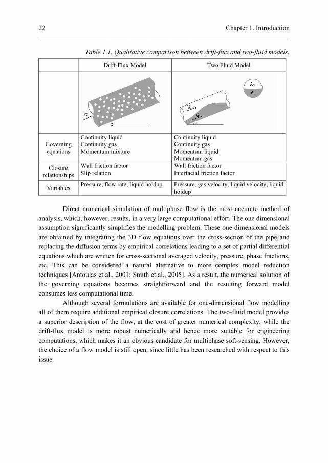
Table 1.1. Qualitative comparison between drift-flux and two-fluid models.
Direct numerical simulation of multiphase flow is the most accurate method of analysis, which, however, results, in a very large computational effort. The one dimensional assumption significantly simplifies the modelling problem. These one-dimensional models are obtained by integrating the 3D flow equations over the cross-section of the pipe and replacing the diffusion terms by empirical correlations leading to a set of partial differential equations which are written for cross-sectional averaged velocity, pressure, phase fractions, etc. This can be considered a natural alternative to more complex model reduction techniques [Antoulas et al., 2001; Smith et al., 2005]. As a result, the numerical solution of the governing equations becomes straightforward and the resulting forward model consumes less computational time. Although several formulations are available for one-dimensional flow modelling all of them require additional empirical closure correlations. The two-fluid model provides a superior description of the flow, at the cost of greater numerical complexity, while the drift-flux model is more robust numerically and hence more suitable for engineering computations, which makes it an obvious candidate for multiphase soft-sensing. However, the choice of a flow model is still open, since little has been researched with respect to this issue.
Drift-Flux Model Two Fluid Model
Governing equations
Continuity liquid Continuity gas Momentum mixture
Continuity liquid Continuity gas Momentum liquid Momentum gas
Closure relationships
Wall friction factor Slip relation
Wall friction factor Interfacial friction factor
Variables Pressure, flow rate, liquid holdup Pressure, gas velocity, liquid velocity, liquid
holdup
Chapter 1. Introduction _________________________________________________________________________
23
1.3. Smart Wells and Soft-Sensing Traditionally, oil production may be divided into three major categories. In the primary recovery phase, the oil is driven out of the hydrocarbon reservoir by its natural pressure, which is considerably higher than the pressure in the bottom of the wellbore, known as bottomhole pressure. Over the lifetime of production reservoir pressure is reduced to a point that it provides insufficient driving force to produce hydrocarbons to the surface, against the effect of friction and gravity. In the secondary recovery phase, water or gas is injected to maintain the pressure in the reservoir at a sufficient level. Other secondary recovery techniques, such as gas lift, reduce the pressure drop in a vertical well, by effectively reducing the density of the fluid in the wellbore. Generally the recovery factor after primary and secondary stages can vary between 30 and 50% [Green, 2003]. Finally, enhanced or tertiary recovery uses a number of sophisticated processes to change the physical properties of the reservoir fluid, allowing additional recovery. The viscosity of the oil can be decreased using thermal influence or the surface tension between oil and water can be altered by the chemical flooding. In recent years, with the extended availability of downhole measurement equipment and actuators the concept of intelligent (or smart) well completions has been introduced. The main application of the smart well technology is to actively intervene in the hydrocarbon production process by means of downhole flow control and sensing [Glandt, 2003]. In particular, such intelligent completions may be used for control of the injection of water or gas in the well to realign the velocity of the injected fluid over heterogeneous layers in a reservoir [Brouwer and Jansen, 2004]. The inflow of certain fluids from different zones in a production well can be limited or eliminated [Aggrey, 2008], which is important for long horizontal, multilateral or other complex wells [Sun et al., 2006]. Intelligent completions are generally based on the following hardware elements: Interval control valves (ICV) and downhole sensors. The well, which is divided in intervals using isolation packers, is equipped with several ICVs which are remotely operated in order to control inflow from different reservoir layers or well branches. In-line separators [Kouba et al., 2006] may be used as down-hole processing units to separate phases. Downhole separation can reduce the energy required to lift fluids to the surface, with the additional benefit of allowing downhole flow metering using single phase meters. Many technological options are available for sensors. The most commonly used sensors are point-pressure and temperature gauges. Alternatively, fiber-optic distributed temperature sensors (DTS) are now widely employed to measure even minor changes in the thermal profile at one-meter resolution with an accuracy of 0.1oC [Brown et al., 2000]. Examples of ways in which such intelligent completions may help production processes on a short-term are:

Chapter 1. Introduction _________________________________________________________________________ 24
– Perform real-time monitoring of production systems and allow remote intervention in production, reducing the need for costly well interventions. An example of this would be water influx, which no longer requires a cement plug, but could be remediated by simply shutting an inflow control valve. - Ensuring optimum production or recovery from a reservoir by including optimization algorithms which take actions based on monitoring data. Examples are optimizing production from various – non-homogeneous – reservoir sections, or improving the sweep efficiency of water flooding by optimizing flow distribution in the reservoir. On the long-term time scale the smart wells are considered as a part of a general intelligent production system, which requires proper management strategy. The difference between production measurements and the output of reservoir/wellbore models is analyzed and used to update the asset within the framework of closed-loop reservoir management (Jansen et al., 2008, Figure 1.5).
Figure 1.5. Closed loop reservoir management after Jansen et al., 2008.
A hydrocarbon system would in principle provide an accurate prediction of the flow variables both in reservoir and wellbore, if that relevant models are perfect. However, the parameters of the system are known to a certain extent only: while the fluid properties of the wellbore fluid are typically accurately known, permeabilities and porosities can vary

Chapter 1. Introduction _________________________________________________________________________
25
greatly throughout the reservoir, but can only be directly measured near the wellbore location. The wellbore flow model also includes a number of unknown parameters (as drift-flux) and the flow regime usually can not be visualized and identified at downhole conditions. In addition to the model parameters the input to the system is not fully defined with the inflow from reservoir to wellbore as a major unknown. The models, which obviously cannot be used alone to describe the performance of the hydrocarbon systems, can be updated in real-time, by estimating the uncertain model parameters and refining the model structure using available measurement output. In the data assimilation concept, the model is updated continuously, when new measurements become available providing estimated values of dynamic flow variables and parameters. These estimates can be used later, for instance, for model-based control of wellbore performance to optimize the production. The controlled inputs can be gas lift injection rate, surface choke settings and downhole flowrates. This optimization acts on a very short time scale and the wellbore response to input change becomes apparent within minutes or hours. The measurements can be either real hardware sensors or soft-sensors, which obtain the production data indirectly. As the data assimilation adapts the parameters of the model to measured data, reliable measurement data are needed. Sensors are required which are designed to operate in aggressive downhole conditions. Nevertheless, faults and breakdowns of downhole equipment can not be completely avoided. Generally, building and maintaining a complex measuring system installed for a hydrocarbon reservoir is quite expensive and depends on the variables to be monitored and data supply frequency. It can be noted that capital costs for intelligent completions vary from USD 200,000 for a permanent downhole gauge system up to USD 2,500,000 for a fully equipped multizone completion with the option of remote control [Robinson, 2003]. There are a number of reasons why the soft-sensors can be used in oil and gas applications. The generally accepted areas of application of the soft-sensing measurement techniques are as follows: 1) Soft-sensors can replace expensive hardware systems, as use of software tools instead of hardware is always a cost reduction. 2) Soft-sensors installed parallel to a measurement device can instantaneously diagnose fault or breakdown of a given piece of hardware equipment and replace it by substituting the missing data by the output of the soft-sensor. This, in turn, allows the use of soft-sensors for real-time estimation for monitoring and control purposes. 3) Validation of the hardware output under normal data conditions. 4) Soft-sensors can be used together with the existing hardware, improving its overall performance. The hardware instrumentation can then operate with increased accuracy, be able to work over wider range of operating conditions, or provide measurement output with a frequency higher than defined by technological capabilities.

Chapter 1. Introduction _________________________________________________________________________ 26
5) The most promising application of soft-sensors, which is especially attractive for hydrocarbon production systems, is the estimation of process variables which are not measured directly. The soft-sensor, or real-time estimator, replaces downhole flow metering and obtains flow rates from conventional downhole sensors, such as pressure or temperature gauges, in combination with a multiphase flow model calculating the quantities of interest with measured data as a basis. The schematic description of soft-sensors for this purpose is depicted in Figure 1.6.
Figure 1.6. Schematic representation of multiphase soft-sensors.
The performance of a multiphase soft-sensor can be described as follows. The hardware equipment measures some flow property, which is not usually the one of direct interest. Even if direct multiphase flow measurements are available downhole, their quality may not be sufficient as the flow meter may fail to provide accurate measurement for a certain flow regime or operate incorrectly over a specific range of flow conditions. However, we present measurements here as general sensors, providing not only flow rates, but also pressures, temperatures, phase fractions and water cuts. Amongst those some measurements are more easily obtained at the surface conditions rather than downhole, though the latter are generally preferred. Downhole data are usually accessible only at few locations.
Available sensors (pressure, Venturi, etc..)
Flow model
Real-time estimator
Flow rate predictions
Model error
Input unknown flow
Measurement noise

Chapter 1. Introduction _________________________________________________________________________
27
Contrary to most sensors, the model can predict the dynamic behaviour of flow variables over the whole simulation domain. However, models used for soft-sensing are usually greatly simplified for real-time operations and the quality of model predictions strongly depends on the empirical closure relations used. Even if the model is perfect, it will only provide accurate prediction of the flow field if the input is known. Given that the input includes the unknown flows, it is not feasible to expect satisfactory model performance, taking also into account other model limitations. Therefore, these two sources of information, model and the measurements, can not be separately used for multiphase flow rate prediction. The soft-sensor combines model and measurement in an intelligent way, aimed at eliminating their drawbacks and reinforcing the strong parts. The multiphase soft-sensor uses the values of dynamic flow variables obtained by a simplified flow model and measured output of downhole equipment installed in the wellbore to provide an estimation of model input and unknown parameters in such a way, that the mismatch between predicted and measured data will be minimized. It should be noted here, that the output of the model and measurements can be completely different, as the soft-sensor provides model based predictions of both measured and unmeasured quantities. For that purposes the dynamic multiphase flow model of the system should be described theoretically, allowing unequivocal predictions of dynamic variables (system output) with a given model input. The best choice is to use the robust, first principle models formulated on the basis of real physical mechanisms, such as drift-flux, two-fluid, etc. Soft-sensing is still an emerging area of research and a very few applications are available which are related to multiphase fluid mechanics. Lorentzen et al., (2003) developed a methodology of tuning of parameters of one dimensional two-phase flow models, in particular for a drift-flux formulation of slug and bubbly flow in vertical wells. The method has been validated employing both synthetic and experimental data, and though the model parameters were not perfectly estimated, the tuning of the model gives an improved performance compared to use of the standard choice of parameters. The estimation was done using the ensemble Kalman filter. In Vefring et al., (2002) a dynamic multiphase well flow model was coupled with a simple transient reservoir model. Using the injections and annulus outlet rates as measurement and the constant bottomhole pressure as the input, the obtained coupled model was used to identify the reservoir permeability using the Levenberg-Marquardt algorithm. It was shown that the simultaneous estimation of permeability and reservoir pressure led to errors in the considered parameters. More recently, Vefring et al., (2006) upgraded the estimation technique by employing the ensemble Kalman filter to perform data assimilation in real time, as new measurements become available, whereas with the Levenberg-Marquardt optimization algorithm all the available data are matched with the output from the coupled model, just as in traditional history-matching.

Chapter 1. Introduction _________________________________________________________________________ 28
Nygaard et al., (2007) proposed an automatic methodology for control of the bottomhole pressure during drilling operations in gas-dominant wells. Besides the control component of the study, the dynamic model of the wellbore flow was calibrated in real-time using available process measurements. The reservoir permeability was updated using the unscented Kalman filter. Leskens et al., (2008) considered the simultaneous estimation of downhole oil, water and gas flow rates from downhole pressure and temperature measurements in a single horizontal well by using the extended Kalman filter. It was shown that in case the measurements are corrupted with noise, obtaining correct estimates is not possible due to bad observability of the system. This allocation technique was further extended by de Kruif et al. (2008) to the multi-lateral well case both for the two-phase (oil and gas) and three-phase (oil, gas and water) cases. It has been shown that for a three phase flow in addition to downhole wellhead measurements are required. The extended Kalman filter was used as a soft-sensor for gas-lift wells by Bloemen et al., (2004). Via simulation based test cases it has been demonstrated that multiphase flow rates can be estimated using pressure measurements along the tubing. Proper estimation of model parameters, i.e. closure for the used drift-flux model, requires additional measurements of liquid flow rate. Muradov and Davies, (2010) considered several soft-sensing methodologies for zonal rate allocation problem, which is based on use of downhole pressure and temperature data. It was shown that in contrast with numerical optimization algorithms, the Kalman filtering is more capable to deal with sufficiently noisy data. Aamo et al., (2005) designed a non-linear observer (soft-sensor) for monitoring the states (gas mass in annulus, gas mass in tubing and oil mass in tubing) of multiphase flow in vertical pipes. The soft-sensors used only topside measurements – the pressure at the top of the tubing and either the flow through the production choke or the density at the top of the tubing. The use of the observer in combination with control algorithms was used to avoid the multiphase instabilities and increase production.
Kalman filtering A classical soft-sensor has three main components. First, it requires the set of conventional hardware sensors which are used to provide data. Secondly, a process model is required. In addition to a flow model, a choice has to be made regarding a data assimilation algorithm, which would relate model predictions with available measurements resulting in estimation of flow variables. One can note two different approaches for incorporating measurement data into the dynamic model: variational data assimilation, which is based on the minimization of a cost function within a certain time interval [Robertson, 1995] and sequential history matching methods or filtering, where the state of the system is updated every time instant new data

Chapter 1. Introduction _________________________________________________________________________
29
become available. One way to solve these sequential data assimilation problems is to use Kalman filter equations [Kalman, 1960]. In order to apply Kalman filtering it is required that the description of model and measurements should be of the form:
1 ( ) ( )k k k k k k k kx A d x B d u v (1.4)
k k k ky H x w (1.5)
Where Ak(dk) and Bk(dk) are the state transition matrices, Hk is a measurement matrix, which relates available observations with model states. x is a state vector, d is a vector of the model parameters and u is a control input (i.e. boundary conditions). Subscripts k and k+1 denote old and new time step respectively. vk and wk are zero mean Gaussian white noise vectors, associated respectively with the model and measurements and characterized by variances Qk and Rk. Initial conditions of the filter are defined by the initial estimate x0 and the initial error of estimation with a known covariance P0. The Kalman filter computes estimates of the state vector which are optimal in a least-square sense for linear system dynamics (eq.1.4). The Kalman filter is a two-stage recursive algorithm, which consists of a prediction step (also called the time update step or forecast step) and a correction step (measurement update or analysis step). With the forecast step, the current filter estimate and corresponding error covariance matrix are used to calculate the prediction based on the model dynamics
1 ( ) ( )f a
k k k k k k k kx A d x B d u w (1.6)
The prediction of the error covariance can be computed as
1
f a T
k k k k kP A P A Q (1.7)
Once the new measurements become available, the model states and the covariance are corrected using this new information.
1
1 1 1 1 1 1 1[ ]f T f T
k k k k k k kK P H H P H R (1.8)
1 1 1 1 1 1[ ]a f f
k k k k k kx x K y H x (1.9)
1 1 1 1( )a f
k k k kP I K H P (1.10)
The superscript f represents the (model) forecasted state of a dynamic system, and superscript a refers to values analyzed by means of incorporating measurement data. Here K is the Kalman gain, which minimizes the covariance matrix P. I is the identity matrix of appropriate dimension. While the error covariance matrix R can in principle be defined from accuracy specifications of the sensors used, the definition of the model error matrix Q is more difficult since the process noise represents the uncertainty in the modelling process itself. It may include the physical simplifications, the uncertainty in numerical algorithm, inaccuracy in boundary conditions, etc. The model error matrix usually acts as a tuning parameter: if the physical model is oversimplified, more confidence in measurement data

Chapter 1. Introduction _________________________________________________________________________ 30
can be granted by choosing a proper Qk. Moreover, a certain choice of the model error matrix can prevent filter divergence for some applications. The important definitions in data assimilation framework are:
1) Model parameters – these variables are usually uncertain and do not change in time, therefore they are also referred to as static variables. For multiphase flows these include fluid properties, such as density and viscosity, wall friction factor, and the parameters of a two-phase flow model (such as drift-flux parameters or interfacial friction factors). If these parameters are explicitly introduced into the data assimilation procedure, the estimates of those are sequentially updated in time, though in fact they still remain constant from the physical perspective.
2) State variables are output solutions from the wellbore simulator, and are updated according to the dynamics of the flow system. Just as the model parameters, the dynamic variables can be poorly defined, by, for example, errors introduced by the numerical algorithm. Additional sources of uncertainty for state variable arise from the link with static parameters defined by the transient model. Model states can be formulated either in terms of conservative variables (phase flow rates, densities) or in a primitive formulation as pressures, velocities, phase fractions.
3) Model input – these are quantities, which, just as static parameters, provide the updated dynamic variables. These are various source terms (mass transfer, pressure drop, inflow, outflow), boundary conditions and, unlike the static parameters, these are usually time dependent. The model input may be affected by the formulation of the governing equations, such as interfacial friction of a two-fluid vanishes when the corresponding momentum equations are added.
4) Measurements are the observable quantities, which are directly related to the state-variables and parameters. For multiphase production system measurements the number of observable states is limited and includes surface flow rates, water cuts, down-hole pressures and temperatures. Obviously the measurement data always have some uncertainty associated with technology and it should be explicitly specified in the data assimilation approach.
Although using the Kalman filter equations one can, in principle, solve many data assimilation problems, the actual implementation for a specific application is not straightforward. First, with the increase of the dimension of the state vector x, the computational effort of the algorithm increases dramatically. The most computationally expensive is the model forecast step, both for model and covariance updates. While for a model update the computational effort is of order n2, the error covariance matrix is updated with n3 operations, which clearly sets a limitation for real-time operation for high-order models. Provided that the wellbore model chosen is robust enough, this is not a main difficulty associated with the use of Kalman filter in multiphase soft-sensors. The update of the error covariance matrix (eq. 1.7) is performed assuming that the original model

Chapter 1. Introduction _________________________________________________________________________
31
equations are linear. Unfortunately, this is not the case for the majority of fluid mechanical applications. The main sources of nonlinearity are caused by the convective transport, and the existence of semi-empirical closure terms. For a general non-linear model process several modifications of the original algorithm have been proposed. The extended Kalman filter (EKF) [Jazwinski, 1970] is a most straightforward extension of the original algorithm to adapt the filter to a non-linear case. It uses the linearization of the given non-linear model around the most recent estimate and, after the linearization, the original Kalman filter equations can be used for forecast and analysis steps. This actually leads to the main shortcoming of the extended Kalman filter approach; its application requires the computation of a Jacobian and hence the EKF may lead to poor results in the case of strongly nonlinear dynamics. More important, the Jacobian can hardly be computed analytically and its numerical calculation greatly increases the computational effort of the filter. Moreover, such numerical differentiation induces additional numerical errors, which eventually diverges estimates from the correct ones. The unscented Kalman filter (UKF) deals with the problem of model non-linearity introducing several sampling points (sigma points) around the current estimate based on its covariance. Afterwards, these points are propagated through the original non-linear process, which provides the estimates of the state vector without complex linearization. Though more accurate, the UKF requires more computational effort and may be computationally unfeasible. The ensemble Kalman filter [Evensen, 1994], is based on a Monte Carlo approach, using an ensemble of possible model realizations to compute the necessary statistics. This method is easy to implement and it handles strong non-linearities better, than other known filtering techniques. There is much ongoing work within different areas of research including petroleum engineering, where the Kalman filter techniques are used. The number of application to wellbore flow is, however, very limited. Therefore it is difficult to conclude which algorithm will perform better as a real-time estimator for a given application and for given flow conditions. While the computational speed is not that important for the one dimensional wellbore model, the quality of the estimates is essential.
1.4. Discussion and Research Directions
Motivated by the growing demand for hydrocarbon production and increased availability of downhole measurement and control equipment, the oil and gas industry has introduced a smart wells concept. The main idea of this approach can be formulated as the improvement of reservoir management by means of wellbore instrumentation and use of various model-based control and optimization strategies. The aim is a higher output from a reservoir both on the short and long term time scales.

Chapter 1. Introduction _________________________________________________________________________ 32
Such strategies in turn strongly rely on the efficiency of downhole equipment, which is used to obtain real-time oil and gas production rates with sufficient spatial and temporal resolution. In particular, multiphase flowmeters installed downhole can improve the production of long horizontal wells by allocating the zones of oil, gas and water inflow. Development of such multiphase flow metering systems (MPFM) has been a major focus of oil and gas industry over the last decade. Although a number of commercially available industrial MPFM systems exist, each of them applies its own technology and principle focused on the specific application. More important, MPFM is quite sensitive to the fluid properties and flow regimes. Furthermore, multiphase flow meters are only accurate within a limited operating range making such real-time monitoring expensive. From the monitoring point of view, the use of sensors which measure different quantities in several locations is preferred. However, because of practical and economical reasons such demands are unrealistic. Moreover, some sensors, like pressure gauges, provide more available measurements than others. To overcome these problems one can use so-called multiphase soft-sensors, i.e. estimate flow rates from conventional meters, such as downhole pressure gauges, in combination with a dynamic flow model. The aim of this research project is to investigate the possibilities and limitations of such multiphase soft-sensors with the focus on gas-liquid flows in horizontal wells. In particular the problems relevant to the development of soft-sensing techniques may be formulated as follows:
1) Since the soft-sensors are model based tools for real-time estimation of unknown quantities, proper flow modelling becomes essential. Such models should be capable to represent the main physics of the process and at the same time should be capable of providing output data in real-time. Either the model should be significantly simplified or the model should be solved by means of robust numerical methods, which allows simulation in real-time or preferably even faster.
2) The choice of the model is also dictated by the type of wellbore flow processes. Obviously the fully dynamic model is more preferred, as it is capable to process the transient signal from the sensor. However, for some formulations the use of a semi-steady state model might be more advantageous.
3) It is important to decide, which set of measurements should be used as an input to a soft-sensor. Some of them, like pressure gauges, supply the operator with information about the flow at multiple locations. As an alternative, distributed pressure sensors can be used which provide continuous both in space and time data regarding pressure distribution in a wellbore. Such sensors, mainly because of their low price and robustness, should be considered as a basis of the real-time estimator. It is also important to decide, which kind of quantities are suitable for indirect measurement of flow rates, as these should implicitly include the information on the flow structure.

Chapter 1. Introduction _________________________________________________________________________
33
4) The soft-sensor algorithms themselves need to be adjusted to the problem considered. Although such methods have been widely used in meteorology [Houtkamer and Mitchel, 1998] and petroleum engineering [Jansen, 2008], very little has been researched with respect to multiphase wellbore flow.
1.5. Outline
This thesis is organized as follows. Chapter 2 gives a detailed overview of the physical model of wellbore flow used. The concept of drift flux is briefly discussed and the closure relations for the governing equations are introduced. In addition, the eigenvalue analysis of the resulting system of equations is performed, which provides characteristics representing the wave propagation speeds in the simulation domain considered. These characteristics are used later to analyze information, which is available for indirect estimation of multiphase flows (Chapter 4). Methods used to the solve model equations numerically are discussed in Chapter 3. It is shown that the traditional central schemes are unable to capture properly the physics of the flow. For the complex flow systems, which include several non-linear coupled differential equations, a new computation algorithm is proposed. First, a Jacobian splitting must be applied accounting for different directions of the propagation of information. Next, the two components of the Jacobian matrix, denoting the positive and negative direction of information propagation are discretized using conventional upwind, accounting for the sign of eigenvalues. Finally, the use of flux limiters is considered, which significantly improves the shock-capturing capabilities of a numerical scheme. Furthermore, the governing equations are reformulated. That allows the numerical upwinding of the source terms, which are included in the state vector. In Chapter 4 an assessment is performed of the impact of the chosen time-integration scheme on results of data assimilation based on the extended Kalman filter approach. The use of the implicit Euler scheme, which is unconditionally stable for the whole range of time steps both for the model and covariance update, results in a less accurate estimation of the permeability distribution, which can be overcome using a parameter estimator based on the explicit Euler scheme. However, the latter strongly limits the maximum time step, which can be used, and leads to inappropriate simulation times. An alternative can be found using a semi-implicit estimator, in which a model is updated using the implicit Euler scheme, whereas the propagation of the error covariance matrix in time is based on the explicit time integration scheme. This hybrid approach combines the accuracy of the conventional Kalman filtering with the robustness of the implicit forward modelling. The proposed algorithm is successfully applied for the solution of the one-dimensional problem of permeability estimation in a porous medium for a single phase oil flow.

Chapter 1. Introduction _________________________________________________________________________ 34
Chapter 5 starts from analysis of the transient pressure signal generated in the wellbore due to inflow from the reservoir. The possibilities of indirect multiphase flow metering are then discussed. Afterwards a real-time estimator is developed, which estimates the liquid fraction distribution for a two phase liquid gas flow from the variation of the frictional pressure drop. The method, which was limited to a rapid inflow scenario, is extended in Chapter 6 to a gas coning control application, in which the relevant quantities are estimated from multiple pressure measurements and single multiphase flow measurement at the outflow. The performance of both techniques proposed is evaluated using a series of simulation based test cases and measurements generated by the OLGA simulator. Finally, Chapter 7 gives conclusions of the thesis and provides recommendations for future work.

Chapter 2. Wellbore flow model _________________________________________________________________________
35
2. Wellbore Flow Model
2.1. Governing equations for a drift-flux model
The equations describing a two-phase one-dimensional flow can be derived from the conservation principles of mass and momentum applied to a control volume of a pipe. The conservation equations are formulated under the following assumptions: 1) Dominant (marching) flow direction does exist. 2) Viscous diffusion in the flow direction can be neglected. The one-dimensional control volume for the gas-liquid wellbore flow is depicted in Figure 2.1. Both liquids are considered as flowing in separate parts of the pipeline with variable cross-sectional area occupied by each fluid. The ratio of the pipe cross-section occupied by the liquid Al to the whole area A is defined by the liquid holdup:
l
l
A
A ; (2.1)
A similar definition of the gas fraction implies that
,
1k
k gas liquid
(2.2)
ds
,,k k ku A
kk
uu ds
s
kk
AA ds
s
kk ds
s
Figure 2.1. Control volume for multiphase flow in pipelines.
The continuity equation for the liquid is derived from the mass conservation principles for a control volume depicted in Figure 2.1. For a constant cross-sectional area A these conservation principles are formulated as
k k k k k
Vk ki
Inflow from mass transfer
reservoir termAccumulated Net mass flow inmass the Control volume
um
t s
(2.3)
Vk

Chapter 2. Wellbore flow model _________________________________________________________________________ 36
Where is the phase volume fraction, is the density, u is the velocity, t denotes
time and s denotes the coordinate along the length of the pipe. Vk is the mass inflow
source per unit volume representing the inflow from a reservoir to the wellbore (Figure 2.2). These sources are normally time dependent. The subscript k denotes the relationship to a given phase and in subsequent equations it will have index either l (liquid) or g (gas). The term mki represents the interfacial mass flow from each of the other phases into a phase k.
Figure 2.2. Schematic representation of horizontal well with inflow from reservoir.
For the case without phase transfer, the continuity equation (2.3) applied for the liquid and gas phases is given by
l l l l l
Vl
u
t s
(2.4)
g g g g g
Vg
u
t s
(2.5)
The momentum conservation written for each phase
2( ) ( )
sink k k k k k k k
k wk ki k k
k
u u p Sg
t s s A
(2.6)
Here p is the pressure, the term wk stands for wall shear stress and ki represents
interfacial interaction. is the pipe inclination angle and Sk is the wetted pipe perimeter.
i

Chapter 2. Wellbore flow model _________________________________________________________________________
37
The general momentum balance for a mixture is obtained by adding the momentum equations for the gas and liquid phases.
2 2( ) ( )l l l g g g l l l g g g
Net force balance on
the Control volumeAccumulated Net momentum in
momentum the Control volume
u u u uF
t s
(2.7)
The equation obtained contains no information on phase interaction. The force balance includes pressure, gravity and frictional components. In the momentum equation for the mixture, the complex interfacial terms are cancelled out.
fr
pF S
s
(2.8)
Here an appropriate model for the frictional pressure losses Sfr is introduced instead of wall shear stress. Equation (2.8) uses a single pressure p for all phases. For different formulations, i.e. multi-fluid models, the use of the same pressure in all phases may cause the model to lose its hyperbolicity [Ransom and Hicks, 1984], which in turn may lead to numerical instabilities. The final form of the momentum equation for the oil-gas mixture is
2 2( ) ( )l l l g g g l l l g g g fr
pu u u u S
t s s
(2.9)
It is necessary to provide a model for the frictional pressure losses Sfr in the momentum equation. A frequently used expression for dispersed type of flows is based on a single phase correlation, with flow variables related to mixture conditions. For detailed description of other flow regimes, for instance slug flow, more complex submodels can be used [Bendiksen, 1996].
2
2fr m m
fS u
d (2.10)
Here d is the pipe diameter and f is the friction factor, which is a function of pipe roughness k and the Reynolds number
Rem m
m
m
u d
(2.11)
With the mixture velocity um defined as
m l l g gu u u (2.12)
And the average mixture density
m l l g g (2.13)
While the density of a mixture can be defined as a linear function of phase fractions, this is not the case for the viscosity. The viscosity of a dispersion is proportional

Chapter 2. Wellbore flow model _________________________________________________________________________ 38
to the viscosity of the continuous phase and depends also on the volume fraction of the dispersed phase and the specific size of the dispersed droplets. For very low gas fraction the Einstein correlation is valid
1 2.5m l g (2.14)
For computational purposes the mixture viscosity can be approximated as the viscosity of one of a continuous phase [Brauner, 1998], e.g.
m l (2.15)
The friction factor for a mixture can be expressed as a function of the mixture Reynolds number, using an empirical correlation for a single-phase fluid. The use and comparison of different friction factor correlations for steady wellbore flow has been given by Ouyang and Aziz, (1996). The friction factor should also be modified for different flow regimes. For smooth pipes and 2000<Rem<105 the Blasius correlation can be used
0.250.316 Remf (2.16)
If roughness k is taken into account the friction factor is defined by the Colebrook-White
equation
1 2.51
2 log3.71Re
k
df f
(2.17)
Formula (2.17) gives f implicitly, therefore iterations are needed to obtain the solution. Alternatively, the Techo formula [Techo et al., 1965] is used, where f is given explicitly as
2
1.964 ln Re 3.8220.868 ln
Re 3.71
kf
d
(2.18)
The use of steady flow friction factors in unsteady problems is adequate only for very slow transients, which may not be valid for certain oil-gas applications. Various transient friction models are available, which split the friction factor in two terms. The first term is calculated using the steady flow friction factor correlation and the second accounts for transient variation of the flow velocities. Transient friction factor is generally represented as
, , , ..tr
u uf f f t u
t s
(2.19)
With the first term in the right-hand side of (2.19) representing steady flow friction factor and the second term is the correction for transient flow. The model for unsteady friction introduced by Brunone et al., (1991) has become the most widely used in applications with fast transients [Ghidaoui et al., 1992]. Though efficient for single-phase flow, the transient friction factor model applied to multiphase flow is not always
Chapter 2. Wellbore flow model _________________________________________________________________________
39
sufficiently accurate. For some applications [Pierre, 2009] transient friction models do not improve model performance predictions compared to the use of only the steady state friction factor correlation. The given set of governing equations is insufficient to fully describe the flow. As there are more unknowns than equations, additional relations are required. The simple thermodynamic closure law prescribes a constant liquid compressibility, while the relation between pressure and gas density is obtained assuming the ideal gas law:
0g gp R T (2.20)
Where Rg is the specific gas constant for the given gas, and T0 is the gas temperature at reference flow conditions. The acoustic speed of sound at adiabatic conditions is defined as [Lighthill, 1978].
0g gc R T (2.21)
Where is the gas adiabatic index.
2.2. Algebraic Slip Model
The use of a single momentum equation instead of separating momentum equations in the multi-fluid approach results in certain difficulties. Since it is usual for the two-phase flow to have some relative motion between liquid and gas, a proper flow description should be in a multi-velocity formulation. As the number of available equations is less than the number of unknown variables, the additional closure correlation is needed to obtain the full velocity field. In a drift-flux approach, as it was proposed by Zuber and Findlay, (1965), the missing information in the momentum equation is given by algebraic constitutive relationship between the velocities of the phases. The drift velocity of the gas phase is defined as the slip velocity between the gas and the mixture
drift g mu u u (2.22)
The weighted mean drift velocity is defined by averaging the local slip velocity over the channel cross section [Ishii, 1975]:
g drift g g g m
g g g
u u u
(2.23)
With <> denoting the averaging operator, defined as
1
A
dAA
(2.24)
Introducing the superficial gas velocity <usg>=<g ug>, equation 2.23 is reformulated as

Chapter 2. Wellbore flow model _________________________________________________________________________ 40
sg g m g drift
m
g g m g
u u uu
u
(2.25)
The distribution parameter C0 and mean drift velocity ub are defined according to equations (2.26) and (2.27) as
0
g m
g m
uC
u
(2.26)
And
g drift
b
g
uu
(2.27)
And the final form of the algebraic slip model is given by
0g m bu C u u (2.28)
With the drift-flux model defined as in equation (2.28) the governing equations are
solved for the primitive set of variables, namely ug, g, l. Other variables of interest can be
unequivocally expressed as combination of these.
Figure 2.3. Profile and local slip mechanisms in the drift-flux model
The obtained analytical slip equation which correlates ul and ug can be replaced by more rigorous models. For example, a more realistic correlation for the slip velocity between two phases can be obtained using the static force balance accounting for different flow regimes. Equation (2.28) sets the gas velocity as a function of the mixture velocity. In order to obtain correct predictions with this model two parameters, namely distribution coefficient C0 and gas drift velocity ub, should be specified properly. Generally these parameters depend on the orientation of the pipeline and on the flow regime.
du
Concentration profile
Gas drift-velocity
Chapter 2. Wellbore flow model _________________________________________________________________________
41
The traditional drift-flux model is formulated for vertical pipelines with dispersed bubble flow. However, the relationship between gas and mixture velocities in the form of equation (2.28) has been confirmed empirically for other flow regimes and other pipe inclinations. The following drift velocity model can be used for slug flow in a vertical pipeline [Davies and Taylor, 1950]:
0.35l g
b
l
gdu
(2.29)
The bubble rise velocity for a bubble flow regime is given by Harmatty, (1960).
0.25
21.53
l g
b
l
gu
(2.30)
While for a vertical flow the drift velocity is caused by the difference between buoyancy and drag forces, in the horizontal flow it is defined by the local axial pressure gradient. The drift velocity was obtained experimentally by Bendiksen, (1984) for various Reynolds numbers in a 2.42 cm diameter pipeline. Franca and Lahey, (1992) obtained the data set on bubble drift-velocity for plug, slug, wavy-stratified and annular flow regimes. A negative value of a drift-velocity for a slug flow was observed. This result was confirmed by Bonizzi, (2003), who, by means of establishing a force balance between pressure and drag forces, has obtained an analytical expression for the slip velocity for horizontal slug flow. In a homogeneous bubbly flow the distribution coefficient C0 is 1 by definition. For other flow regimes the distribution coefficient ranges from 1.0 to 1.25. Various models for C0 have been proposed for different flow conditions. The simple correlation, introduced
by Ishii, (1977) C0=1.2-0.2.(g/l)0.5 accounts for inertia effects and is valid for a wide
range of Reynolds numbers. The limiting case with equal densities, corresponding to homogeneously distributed fluids, leads to the distribution parameter of unity. For low gas concentrations, the distribution coefficient should have a near-one value. This is taken into account by introducing the void fraction into the existing correlation. Equation 2.31
describes the development of two phase flow for gas fraction g<0.25. Beyond this range
C0 is equal to its standard value for the developed flow. The influence of the void fraction on the distribution parameter was also studied by Clark et al., (1990)
0( 18 )1.2 0.2 1 e
g
l
gC
(2.31)
The Collins correlation [Collins, 1978], which was obtained for slug flow in vertical pipelines, includes the effect of flow homogenization at high Reynolds numbers. As the velocity and concentration profiles become uniform the value of Co approaches 1.0.

Chapter 2. Wellbore flow model _________________________________________________________________________ 42
0
log(Re ) 0.089
log(Re ) 0.74
m
m
C
(2.32)
A more recent drift-flux model [Shi et al., 2003] defines the distribution for a certain range of void fractions in slug and bubbly flow, which approaches 1 as the void fraction exceeds some threshold value B
0
21 1
AC
A
. (2.33)
Here A is the constant value of C0 for a given flow regime and is the term
depending on g
1
g B
B
(2.34)
More drift-flux correlations exist for different applications. A review and assessment of the predictive capabilities of the most commonly used models is given in Coddington and Macian, (2001). The use of these correlations leads to continuous and differentiable models which can be directly used for multiphase flow simulation. However, from a computational point of view, the use of constant drift flux parameters seems to be more reasonable. Based on equation (2.31) the standard value 1.2 for C0 can be used for bubbly flow if the density corrections are ignored and the multiphase flow is developed. For a horizontal stratified flow the value of C0 is close to 1, while it is about 1.15 for the slug flow regime. Experimental data [Chen, 2001] can be used to update existing values for drift-flux parameters or to obtain those for other flow patterns or pipe inclination angles.
2.3. Matrix form of conservation equations
The system of partial differential equations (2.4), (2.5) and (2.9) can be written in a compact form as
U F
Qt s
(2.35)
Where U is a vector representing the unknown conservative variables, F is the vector of fluxes and Q is a vector of source terms. For equations (2.4), (2.5) and (2.9) these variables are defined according to
( )
l l
g g
l l l g g g
U
u u
; 2 2
l l l
g g g
l l l g g g
u
F u
p u u
;
l
g
fr
Q
S
(2.36)

Chapter 2. Wellbore flow model _________________________________________________________________________
43
Equation (2.35) can be equivalently represented in a quasi-linear form using the Jacobian matrix A=∂F/∂U
U U
A Qt s
(2.37)
The additional equation for the gas velocity is taken from the algebraic slip relation (2.28). Obtaining the Jacobian is not a straightforward task as it is difficult to compute the derivatives of the flux components with respect to variables. Obviously, the choice of the conservative variables U is not a convenient one due to different aspects. First, the closure equations for the drift-flux model are formulated in terms of the primitive variables (i.e. density, velocity, liquid holdup) and, therefore, the numerical solution based on a conservative variable set needs extra iterations to perform a conversion for the primitive variables for each time step. More important, the output of the sensors is usually expressed as a function of the primitive variables (see chapter 1). In order to match both the model and measurement predictions additional mathematical operations are needed. This may decrease the accuracy of the existing prediction, as the error in estimation propagates through the computation algorithm. An alternative formulation of the model can be written in terms of primitive variables. The following set of primitive variables is suggested.
T
g g lW u (2.38)
This choice of variables is not unique and one can, in principle, use pressure instead of gas density, liquid velocity instead of gas velocity and void fraction instead of liquid holdup. In addition to the choice of the variables, special attention should be given to
the liming case of single phase gas flow, since equation (2.28) has a discontinuity at l=0.
Using (2.38) the matrix form of the governing equation is converted to
U W F W
QW t W s
(2.39)
Or
1 1
U F U
W WA A A Q
t s
(2.40)
Where AU=∂U/∂W and AF=∂F/∂W
The product of 1
UA and FA is the actual Jacobian of the system, written in terms of the
primitive variables
W W
A Qt s
; (2.41)
Where
1
U FA A A (2.42)

Chapter 2. Wellbore flow model _________________________________________________________________________ 44
1
UQ A Q (2.43)
Transformation from the conservative to the primitive variables is defined by the Au transition matrix. Equation (2.41) can be rewritten using the definition of Au as
1 1
U U U
W WA AA A Q
t s
; (2.44)
Therefore, the transition between the model Jacobian expressed in terms of the conservative and primitive variables is given by
1
U UA A A A (2.45)
The model (2.43) is considered to be well-posed if it appropriately reflects the physics of the flow. Equally, the eigenvalues of the Jacobian should be real and distinct [Ishii and Song, 2000]. The eigenvalues are obtained from solution of the following system
det[ ] 0A I (2.46)
Substitution of matrix (2.42) into (2.46) gives a cubic polynomial equation for the
eigenvalues , which provides three solutions. Eigenvalue analysis of the drift-flux model
has been performed by Theron, (1989) and Gavage, (1991) under the assumption that the liquid phase was incompressible.
The eigenvalues of A matrix are given as follow
1 gu (2.47)
2 ,3
0
0
11
g
l g
g l m
u c
CC
(2.48)
Equation (2.48) can be reformulated as follows
2 ,3 2l phu u (2.49)
Where u2ph is a speed of sound in the gas-liquid mixture.
2
0
0
11
g
ph g
g l m
u c
CC
(2.50)
The obtained eigenvalues of the jacobian A or characteristic speed define the physical behaviour of the multiphase system. Since all the three eigenvectors are real and distinct, the system of the equations for transient two-phase flow is hyperbolic. On a physical basis eigenvalues represent speeds with which information is propagated in the domain. Two characteristics are running in the flow direction and one in opposite if the liquid velocity ul is less than a speed of sound in the gas-liquid mixture u2ph. In general the information may propagate in as many directions as there are eigenvalues obtained.

Chapter 2. Wellbore flow model _________________________________________________________________________
45
Expressions similar to (2.48)-(2.50) can be derived for homogeneous flow with a single velocity, where the liquid compressibility is taken into account
1 f
f
Tp
(2.51)
The speed of sound in the liquid phase is
1
l
l l
c
(2.52)
Using the similar analysis as for the drift-flux model the following expression is obtained.
2
2 2
1ph
g l
m
g g l l
u
c c
(2.53)
Equation (2.53) represents the velocity of sound in a homogeneous two-component mixture, and it was first introduced by Wood, (1941). It can also be obtained as the limiting case of equation (2.50) with C0=1 if liquid is incompressible. In addition to Wood’s formula several attempts have been made to establish multiphase speed of sound for more general flow cases. Nguyen et al., (1980) developed a similar model to predict the sonic velocity for stratified and slug flow regimes. For a case in which the gas and liquid velocities are different Henry, (1970) introduced a corrected formula using a slip relationship. On the other hand, the propagation properties are affected by the mathematical formulation of the flow model and the speed of sound is extracted from eigenvalues of the formulated system. Theoretical predictions of the phase sonic velocities in the two-phase mixture from the eigenvalues analysis have been given by Lee et al., (1998) for the two-fluid model. It should be noted that only closure equations in differential form affect the characteristics of the system [Evje and Flatten, 2007]. Any input to the system, such as variation in a liquid holdup or velocity is transmitted through the pipeline with a certain speed, which is defined by the eigenvalues of the mathematical model. Wave attenuation is another source of uncertainty that influences the dynamics of the two-phase flow. The main mechanism for pressure wave attenuation in pipelines is diffusion, which for the one-dimensional approach is approximated by a friction factor (steady or unsteady) [Pierre and Gundmundsson, 2009]. The main attenuation mechanisms for liquid-gas flows have been analyzed by Falk, (1999). The number of characteristics or eigenvalues or waves is different for various model formulations and defined by the number of dynamic equations used. That may range from two eigenvalues for the simple isothermal pseudo single-phase model to six for a 1D thermal two-fluid formulation. If the dynamic behaviour of certain variables is disregarded,

Chapter 2. Wellbore flow model _________________________________________________________________________ 46
the corresponding equation is replaced by an algebraic relation, which decreases the number of characteristics. For gas-liquid flows in pipelines it is possible to define two classes of physical phenomena, namely convective transport and pressure wave propagation. Fluid convection is characterized by the first eigenvalue and characterized by the local velocity of the gas phase. The second and third eigenvalues correspond to pressure wave propagation both in the direction coinciding with flow and counterflow (if ul<u2ph). In a typical two-phase flow problem, the characteristic time scale is of the order of 10-3s for dynamic waves and 10-1s for convective waves. The latter, however, is not the fastest phenomena as phase transitions (evaporation, boiling), which are omitted here, occur on the time scale of 10-5s [Stewart and Wendroff, 1984]. Normally these pressure waves are not influenced by kinematic wave propagation, as was pointed out by Falk, (1999) and Boure, (1997). The speed of sound in the two-phase mixture is much smaller than both single phase liquid or gas flows. Plotting mixture speed of sound as a function of the liquid holdup for typical values of flow parameters will result in the following graph (Figure 2.4).
Figure 2.4. Speed of sound of a two-phase mixture as a function of liquid holdup for a
homogeneous air-water mixture at 1, 10 and 100 bar. Although the mixture speed of sound is considerably smaller than the speed of sound in one of the pure components over a wide range of flow conditions, it increases dramatically for the liquid holdup values of 1 (pure liquid) and 0 (pure gas), producing strong nonlinearities. As for majority of flow applications u2ph>>ul, ug the influence of convective
0
100
200
300
400
500
600
700
800
0 0.2 0.4 0.6 0.8 1
Liquid Holdup, [-]
Sp
ee
d o
f s
ou
nd
, m/s
p=1 bar
p=10 bar
p=100 bar

Chapter 2. Wellbore flow model _________________________________________________________________________
47
transport on the pressure wave propagation can be neglected. This, in turn allows to leave out the acceleration terms in the mixture momentum equation. For the case in which the convective acceleration is neglected, the transformation matrices of the system AF and AU are formulated as follows
0
0 0
1 0
1(1 ) 1
l
U l g
l g l m g l g
A
u uC
(2.54)
and
0
0
2
0 (1 (1 ))
(1 ) (1 )
0 0
l
l l g
F l g l g g g
g
C uC
A u u
c
(2.55)
With corresponding eigenvalues of 1
U FA A A given as follows
1 gu (2.56)
2 ,3 2 Phu (2.57)
Where u2ph is the expression for the speed of sound of the two phase mixture which is defined by an expression similar to equation (2.50).
2.4. Summary The model for the simulation of the liquid-gas flows in horizontal wellbores has been formulated. The main advantage of the drift-flux approach is that the governing equations are given in conservative form, which makes them easy to solve using conservation numerical methods. The mathematical model given by (2.37) is hyperbolic for a wide range of flow parameters with three real and distinct eigenvalues. Two of these characteristics represent high-speed pressure waves propagating both in upstream and downstream direction of the flow. One characteristic corresponds to void fraction waves and coincides with the velocity of the gas phase. The following assumptions are suggested in order simplify the proposed model: - Liquid is treated as incompressible, whereas the gas density is related to a single fluid pressure using the equation of state for the ideal gas.

Chapter 2. Wellbore flow model _________________________________________________________________________ 48
- It is reasonable to neglect acceleration terms from the mixture momentum equation as these do not have a significant influence on the flow phenomena over range of flow conditions of interest. - Despite the variety of drift-flux models available, the simplest one should be used as a prototype of a soft-sensor. Here the model with constant distribution coefficient C0 and bubble drift velocity is used. - The sources representing the inflow from reservoir to wellbore (Figure 2.2) are assumed to be independent from the dynamic flow variables. However, they can be transient and act as the external input to the system. - Despite the variety of correlations available for wall frictional losses, both steady-state and transient, the one proposed by Techo is used. The system of partial differential equations describing the flow has to be supplemented with initial and boundary conditions. For the hyperbolic problems the choice and formulation of boundary conditions depends on the directions of the characteristics at the boundary. Therefore it will be discussed in more detail in the next chapter.

Chapter 3. Numerical methods _________________________________________________________________________
49
3. Numerical Methods
3.1. Introduction
With the governing system of equations formulated in terms of the partial differential equations (2.4), (2.5) and (2.9), the relevant state variables are formulated as a function of continuous axial coordinate s and time variable t. To enable the use of a Kalman filter or other data assimilation algorithm, the model should be converted in a discrete state-space form, in which the output of the model is defined as a function of the current system state and the input. This formulation can be obtained by establishing a forward solution algorithm. As the analytical solution is not available due to complexity of the drift flux model, the equations governing the flow are solved numerically. Despite the variety of numerical schemes available all of them imply the spatial discretization of the simulation domain into a finite number of grid blocks or control volumes and subsequent integration of the governing equation over these grid blocks. The resulting discrete state variable has the form of a state vector
1 2[ .. ]k k k Nk
Tx x x x (3.1)
Where xik is the state variable defined in the grid block i and evaluated at the time level k. After the discretization of the computational domain the following system of ordinary differential equations is obtained:
,t
t t
dxF x u
dt (3.2)
The general solution of equation (3.2) for one time step is given by
1
1 ( , )k
k k t t
k
x x F x u dt
(3.3)
The mathematical method to be used for the soft-sensing is formulated in the following state-space form
1 ( , )k k kx f x u (3.4)
Where the operator f(.) represents a general solution of the ordinary differential equation. This operator is usually not available in a direct form as it depends on the numerical algorithm used. Although during the last decades an enormous amount of robust, efficient and accurate solvers have been developed for one-dimensional modelling of single-phase compressible flow, the achievements for its multiphase counterpart have been less impressive. Due to the difficulties related to modelling of multiphase flows, such as presence of non-conservative terms, flow regime dependency, etc., the development of the

Chapter 3. Numerical methods _________________________________________________________________________ 50
multiphase numerical algorithms is generally more intricate and complex. The numerical methods currently used for multiphase flow modelling are recognized to possess certain drawbacks to accurately predict flow performance. Depending on the problem, the required accuracy, and the availability of the computational resources, one can choose among a range of well-establishing techniques to obtain the numerical solution. In Godunov-type methods [LeVeque, 2002] the exact solution for the local Riemann problem is obtained at each grid interface. The usage of this technique requires the algebraic expression of the physical flux F, which may not be available due to the complexity of submodels used in the drift-flux formulation [Baudin et al, 2005a]. However, several attempts have been made in order to build the solver by using extensions of the original algorithm. A scheme introduced by Romate, (1998) uses a numerical approximation of the physical flux, while its analytical expression for a specific formulation of an algebraic slip model is given by Faille and Heintze, (1999) and Flatten and Munkejord, (2006). In contrast, central schemes [Toro and Bilett, 2000; Chen and Toro, 2004] do not explicitly account for the direction in which information is propagated, and its usage is convenient for incorporating additional closure equations. In a flux-splitting approach [Evje and Fjelde, 2002], the convective terms are divided into parts corresponding to positive and negative eigenvalues. This method will be discussed in detail later on in this chapter and implemented in a flow simulator. Unfortunately, there are no direct recommendations available for the choice of the relevant numerical scheme for multiphase soft-sensing. It is appealing, however, to use the flux splitting methods as they are usually simpler to implement. Generally the aspects, which are important for selecting the appropriate numerical method for wellbore flow, are directly related to the terms in general conservation equation (2.37), namely, transient, convective and source. 1) For the transient term a choice has to be made between explicit and implicit schemes. The use of implicit schemes is normally beneficial from numerical stability considerations, as it imposes no numerical stability restriction on the value of the time step used. However, the use of the very large time steps can disregard the flow phenomena acting on a very small time scale and smear out discontinuities [Toumi, 1996]. For the cases in which the pressure wave propagation is less important than convective transport, the semi-implicit time integration is introduced [Baudin et al., 2005b]. It treats the dynamic waves implicitly, whereas the treatment of mass transport, which defines the maximum allowed time step, is explicit. The influence of the time integration scheme on the results of data assimilation is studied in detail in the next chapter. 2) Another important issue is related to the representation of the convective terms. Depending on how the numerical flux function is defined, one can distinguish between central and upwind schemes. The first category produces numerical oscillations in the vicinity of a wave front, while the second generates numerical diffusion which smears out

Chapter 3. Numerical methods _________________________________________________________________________
51
step gradients. The development of the computational techniques tends to reduce the unphysical oscillations and numerical diffusion and increase the accuracy of the scheme. Multi-step schemes [Liska and Wendroff, 1999] consist of time step based on a second order schemes followed by time step of a first order. The use of these compositional schemes reduces both numerical instabilities and numerical diffusion. These schemes, which are quite easy to implement in forward modelling, are generally not recommended to use for data assimilation purposes, as they tend to increase the size of the state vector, which should be augmented with these intermediate time steps [Madsen and Canizares, 1999]. Recent developments in the shock capturing schemes, which do not produce unphysical behaviour at the front of the wave propagation and allow to obtain accurate results with a reduced number of grid blocks, seem to be promising from the soft-sensing perspective. 3) The existing numerical algorithms to be used with convection dominating problems were initially developed for homogeneous equations. This is not the case for multiphase models, as the sources will always be present in a drift-flux formulation. Numerical difficulties associated with incorrect source term treatment, especially with regards to obtaining a correct solution, have been reported by several authors [LeVeque, 1998; Koren, 1993]. A commonly used solution for non-homogeneous governing equations is based on the fractional step splitting where first a homogeneous problem is solved and then a correction step is applied in order to add the influence of the source [Toro, 1999]. This approach, however, may easily fail if the transient term is small compared to convective and source term contributions, that corresponds to a solution close to a steady-state [LeVeque, 1998]. Numerical schemes based on the flux splitting, which lead to accurate solutions of non-homogeneous conservation equations, have been proposed. In [Hubbard and Garcia-Navarro, 2000] a discretization scheme which balances the source terms with convective fluxes, was introduced. This balance was achieved by Bermudez and Vazquez, (1994) and Chacón Rebolo et al., (2002) by reformulating the set of governing equations and numerical upwinding of the source terms. In Gascon and Coberan, (2001) the non-homogeneous equations have been transformed into homogeneous by introducing a new flux vector. The purpose of this chapter is to provide a brief description of basic numerical algorithms used for the multiphase flow simulations. First, a brief overview of the numerical schemes used for convection dominated problems is given. After that, the problem of proper source term treatment is introduced and a special correction algorithm is proposed. The last section deals with validation of the chosen numerical strategy. The wellbore simulator is validated against benchmark cases and data generated by the well-established commercial simulator OLGA. Finally, the chapter ends with conclusions.

Chapter 3. Numerical methods _________________________________________________________________________ 52
3.2. Discretization of the flow equations
General formulation The drift flux model defined in the preceding chapter is described by a system of conservative equations:
( )( )
Source
termTransient Convective
term term
U F UQ U
t s
(3.5)
Where U is a vector of conservative variables, F is a vector of flux variables and Q is a vector of source terms, which is represented by algebraic functions of conservative variables. The quasi-linear form of the equation (3.5) is given by
U UA U Q
t s
(3.6)
Basic principles The first step in formulating a numerical method to solve the system in the form of equations (3.5) or (3.6) consists of discretization of the simulation domain (Figure 3.1). The
mesh is composed of grid blocks with si=0.5(si+1/2+si-1/2) the cell centers and si=si+1/2-si-1/2
the grid block length. The discrete values of dynamic variables are located at the centers of these gridblock, so Ui=U(si) is the value of conservative variable associated with ith grid block.
s
is
1/ 2is
Figure 3.1. Discretization with notations.

Chapter 3. Numerical methods _________________________________________________________________________
53
With the uniform grid spacing and the use of a fully explicit time integration scheme, the system of non-linear algebraic equation is obtained, which represents the conservation properties of dynamic variables in control volume. For a system written in conservative form, the discrete equation for a grid block is
11 / 2 1 / 2
k k k k ki i i i i
tU U F F t Q
s
(3.7)
Where t is the time step, s is the grid block length, F is the numerical flux
which represents the physical flux defined at the cell interface, subscript i represents the cell index. An expression for the interface flux F is required, which is determined by the particular choice of a numerical scheme. This can be performed using standard schemes (first or second order upwind or central difference) or employing more rigorous high-resolution algorithms. The mathematical fundamentals for solving equation (3.7) have been first obtained from the analysis of scalar hyperbolic conservation laws. Although the extension of the scalar scheme to its vector counterpart may not be straightforward, it is convenient to formulate basic expressions of the numerical flux F for the simplest flow model. For example, the one dimensional, linear advection equation without a source term is given by
0u u
at s
(3.8)
Equation (3.8) describes the propagation of a wave u with a constant speed a. The discrete form of (3.8), similar to (3.7) is written as
11 / 2 1 / 2
k k k ki i i i
tu u a u u
s
(3.9)
Numerical solution of linear advection equation Equation (3.8) is hyperbolic: the solution in a given location should only depend on the information upstream that point. Formulations, which do not take into account the flow direction are either unstable or require compensational terms. The upwind scheme accounts for the direction in which information is propagated by evaluating the interface value of u at its upstream neighboring grid value
1 / 2i iu u (3.10)
The use of the upwind discretization leads to a numerical scheme which is first-order accurate in space. The main disadvantage of the upwind type of scheme is numerical diffusion which tends to smear out wave phenomena. The value of the numerical diffusion is proportional to the size of a grid block and it may be a severe limitation of the use of the upwind schemes. The error caused by the first order accuracy of the upwind scheme can be minimized by extending the discretization to a higher order. These schemes use more grid

Chapter 3. Numerical methods _________________________________________________________________________ 54
points to calculate the intercell flux and are therefore more accurate. Some examples of the widely used high-order schemes are second order upwind
1 / 2 1
1
2i i i iu u u u (3.11)
And the third order upwind scheme, which is also referred to as QUICK scheme [Leonard, 1979]
1 / 2 1 1 1 1
1 12
4 8i i i i i i iu u u u u u u (3.12)
The three chosen numerical schemes are assessed for the following test case where a block wave of 0.5m length is transmitted through the simulation domain with a constant velocity a=0.1 m/s. The pipe length is 1m and it is discretized with a 100 gridblocks of a constant length. The comparison of the results obtained by three upwind based schemes with the analytical solution is depicted in Figure 3.2 at t=5s and in Figure 3.3 at t=7.5s. All the employed schemes used a constant time step value of 0.01s.
-4.0
-2.0
0.0
2.0
4.0
6.0
8.0
10.0
12.0
0 0.2 0.4 0.6 0.8 1
Pipe length, m
u, m
/s
UD
UD 2nd Order
QUICK
Analytical
-4.0
-2.0
0.0
2.0
4.0
6.0
8.0
10.0
12.0
0 0.2 0.4 0.6 0.8 1
Pipe length, m
u, m
/s
UD
UD 2nd Order
QUICK
Analytical
Figure 3.2. Results for linear advection
problem, t=5.0 s, N=100 cells. Figure 3.3. Results for linear advection
problem, t=7.5 s, N=100 cells. It can be noted that though the upwind scheme predicts the general behaviour of the flow correctly, the front of the wave is smeared out. As the wave propagates into the simulation domain, the artificial diffusion further smoothens the discontinuity. This is also illustrated in Figure 3.3, where the slopes of fore and rear fronts of the block wave are different. The use of the schemes of higher order resolves the rapid varying regions of the flow much better. However, the regions of discontinuity are corrupted by wiggles, which overshoot and undershoot the exact solution. It is more apparent for the case of second

Chapter 3. Numerical methods _________________________________________________________________________
55
order upwind scheme, where the initial profile oscillates in the vicinity of the discontinuity. The third order scheme is much better in this respect: though it resolves the shock interface with moderate smearing, on the other hand it shows more monotonic behavior compared to its second order counter part. In both cases, the solution exceeds the values set by initial bounds, where in some locations near the wave front it becomes negative. If the dependent variable u cannot be negative from physical considerations, the use of high-order schemes is not recommended. It seems logical to combine the monotonic properties of first order upwind scheme and accuracy of the high-order discretization and suppress at the same time the induced numerical oscillations. In particular, high resolution schemes may be considered as a natural extension of the mentioned approach, which increases the performance of numerical scheme.
High-resolution scheme One can obtain a high resolution scheme by combining a standard scheme of the first order with a high order scheme and introducing special functions which limit numerical oscillations to physical values. It is generally accepted that high-resolution scheme should possess the following properties [Hirsch, 1990]:
1) Provide 2nd order (or higher than second order) accuracy in resolving interfaces, shocks and discontinuities.
2) The amount of grid points can be reduced dramatically maintaining at the same time the same level of accuracy.
3) Prevent numerically induced oscillations. The general expression for a high resolution numerical flux is given by [Sweby, 1984].
1 / 2 ( )HR LO LO HOi i i i iF F r F F (3.13)
Where FLO is a flux defined by low order scheme, FHO is a flux defined by high
order scheme. And is the flux limiter, which sets the ratio between different schemes
depending on the gradients near a particular grid block ri. For a positive flow direction ri is defined by the following expression
1
1
i i
i
i i
u ur
u u
(3.14)
Three flux limiting functions have been studied: MinMod, SuperBee and Van Leer. The mathematical expressions of these flux limiters [Wesseling, 2001] are given in Table 3.1. The use of flux limiting is illustrated in Figures 3.4-3.5. The same initial data as in the previous case have been used. As it follows from the figures the use of flux limiters introduces a significant improvement in the numerical solution. Two observations can be made. First, the solution is monotone, i.e. no unphysical behaviour is observed in any

Chapter 3. Numerical methods _________________________________________________________________________ 56
location of simulation domain. Secondly, the accuracy of the front tracking is much better than for all schemes considered so far.
Table 3.1. Flux limiting functions for the case study
Flux Limiter Equation
MinMod max[0, min(1, )]r
SuperBee max[0, min(1, 2 ), min( , 2)]r r
Van Leer ( ) /(1 )r r r
For that particular problem the SuperBee limiter seems to work in a superior way. It should be noted that the use of the explicit time integration scheme simplifies greatly the programming issues related to the implementation of flux limiters. For an implicit formulation, the solution of a system of non-linear equations is required.
-2.0
0.0
2.0
4.0
6.0
8.0
10.0
12.0
0 0.2 0.4 0.6 0.8 1
Pipe length, m
u, m
/s
MinMod
SuberBee
Van Leer
Analytical
-2.0
0.0
2.0
4.0
6.0
8.0
10.0
12.0
0 0.2 0.4 0.6 0.8 1
Pipe length, m
u, m
/s
MinMod
SuperBee
Van Leer
Analytical
Figure 3.4. Results for linear advection
problem, t=5.0 s, N=100 cells. Figure 3.5. Results for linear advection
problem, t=7.5 s, N=100 cells.
Flux splitting scheme It has been shown that with the use of the upwind scheme the relevant physical phenomena are automatically incorporated into the discrete equations. Although straightforward in the scalar case, the upwinding becomes different when more than one equation is used. The adaptation of the upwind scheme to a system of equations describing the multiphase flow may be achieved with the least effort by using the flux splitting approach.

Chapter 3. Numerical methods _________________________________________________________________________
57
In the flux splitting approach the non-conservative form of the governing equations is considered. For the sake of clarity, the source term is assumed to be zero.
0U U
At s
(3.15)
For the case of general conservation laws with multiple eigenvalues it is appealing to use the knowledge of the direction in which information is propagated. Upwind scheme can then be used for the processes described by the positive eigenvalues and downwind for the negative. In the numerical methods that concept may be realized by splitting the Jacobian matrix in two parts, with one having positive eigenvalues and another having negative ones. The Jacobian matrix A can be represented as
1A T T (3.16)
Where [] is the diagonal matrix formed by the eigenvalues of A, namely
1
..
N
(3.17)
Then [] may be split as
(3.18)
And a natural splitting of A results in
1 1A A A T T T T (3.19)
Now the quasi-linear form of the model equation is given by
U U U
A A Qt s s
(3.20)
And the formulation in terms of primitive variables is
W W W
A A Qt s s
; (3.21)
In equation (3.21) /A U s corresponds to a flux in the direction coinciding
with the flow, which is defined by the positive eigenvalues of the system. Therefore the
terms /A U s and /A W s should be approximated by the upwind scheme, as the
information to a grid block i is coming only from upstream direction. Similarly, the terms associated with the negative eigenvalues should be treated with downwind scheme.
1 1i i i i
i
U U U U UA A Q
t s s
(3.22)
The discretization of other formulations is performed in a similar way. The expression for the intercell flux, which has two flux contributions from neighbouring cells, reads then

Chapter 3. Numerical methods _________________________________________________________________________ 58
1 / 2 1 1i i i i if f U f U (3.23)
These fluxes should be defined in terms of components of the discrete equation (3.22), as the operations of splitting and introducing the quasi-linear form do not commute, i.e.
f
AU
;f
AU
(3.24)
1i
1 1i iF U i iF U
i 1i
Figure 3.6. Definition of the numerical flux in flux splitting approach.
With the obtained discrete equation for the numerical flux the corresponding high resolution scheme can be constructed. The main difference from the scalar case is in introducing the additional flux limiting function for the counterflow direction. The expression of the downwind high resolution numerical flux is similar to its upwind counterpart.
Time step size With the numerical fluxes evaluated on the old time level the stability of the numerical scheme is prescribed by the CFL (Courant-Friedrichs-Levy) condition
1 2max( , .. )N
st CFL
(3.25)
Where the CFL limiting value should not exceed 1. The denominator of (3.25) is the largest speed of sound of the model and for drift-flux flow it is defined by dynamic wave propagation.
Boundary conditions For a hyperbolic system of equation it is important to account for information which leaves and enters the computational domain through characteristics. The
characteristics represented by 1 and 2 transmit information in positive direction. These
characteristics leave the information from the simulation domain at the outlet. The wave,
represented by the 3 travels in the negative direction and takes the information out of the
simulation domain at the inlet. These outgoing characteristics give additional information which is used in formulating the boundary conditions.

Chapter 3. Numerical methods _________________________________________________________________________
59
1i 2i i N1i N
3
2
1
Figure 3.7. Determination of boundary conditions. Left – inlet boundary cell, right outlet
boundary cell.
Alternatively, the missing information can be obtained from various numerical boundary conditions, where dynamic variables of interest are extrapolated in a special way near the boundary. This technique may not produce as accurate results as with direct calculation of states at the boundary, though it is much simpler to implement.
3.3. Numerical Example. Need for source term correction In order to evaluate the numerical tools the following test case is considered. A gas liquid mixture is flowing in a horizontal pipeline of 100m length. After a certain period of time additional fluids starts entering or leaving the pipeline at multiple locations. This problem is illustrated schematically in Figure 3.8 with the initial data given in Table 3.2.
Table 3.2. Initial data for numerical example
Quantity Value Pipe diameter, m 0.05 Pipe length, m 100
Mixture speed of sound, m/s 100 Mixture viscosity, Pa.s 0.001
Mixture reference density, kg/m3 11.93 Gas viscosity, Pa.s 1.82.10-5
Inlet flow rate uS, kg/s 0.10 Pipe roughness, m 0.0
The objective of this simple case is to evaluate the abilities of the chosen numerical algorithm to deal with the inflow from the reservoir. The influence of the
reservoir on the wellbore dynamics is represented by the inflow sources l and g. For the

Chapter 3. Numerical methods _________________________________________________________________________ 60
homogeneous no-slip model, in which the continuity equations are added up, a single
inflow source is introduced. The total amount of fluid entering the wellbore is alternated
by the same amount which leaves it. It is assumed that the absolute value of the inflow source is comprised of 0.1 kg/s of liquid and gas. These sources are disabled in the initial stage of simulation process and activated after 5 seconds of flow.
l gF F
,t s
0.1
5
Figure 3.8. Sketch of the simulation domain with sources.
Although the numerical techniques developed are mainly designed for transient multiphase flow simulation, it is also important to check the stability of the steady flow solution. For the sake of simplicity a simple flux splitting scheme without flux limiters has been employed. The steady flow distribution of the gas density obtained after 20 s of simulation is depicted in Figure 3.9.
10.0
11.0
12.0
13.0
14.0
15.0
0 20 40 60 80 100
L, [m]
Rh
o, k
g/m
3
t=4s
t=6s
t=20s
Figure 3.9. Simulated gas density for homogeneous equilibrium model.

Chapter 3. Numerical methods _________________________________________________________________________
61
It can be noted that the obtained density profile is far from physically correct. One can observe multiple local variation of the solution, where the inflow/outflow source is present. These numerical artefacts have a purely numerical origin and they have been generated via the discretization error in the treatment of the source term. Moreover, this density variation corresponds to a steady flow solution of the system, and it is apparent from the figure that it is not influenced by the dynamics of the flow. In order to evaluate the capabilities of the existing numerical scheme to handle the source terms and estimate quantitatively the error induced by the numerical scheme an analysis is performed. Here a simple steady equilibrium model with negligible friction and transient terms is considered.
( )m us
(3.27)
0p
s
(3.28)
Or in a compact form
F
Qs
(3.29)
With
m
m
Uu
; mu
Fp
;0
Q
; (3.30)
The subscript m refers to the variables evaluated at the mixture conditions. In subsequent analysis this index is omitted. The simulation domain is sketched in Figure 3.10. We are seeking the numerical solution in the vicinity of the inflow source. The discrete grid has the following structure (Figure 3.11).
inletF
1i 1i i
i
Figure 3.10. Simulation domain for
introductory test case. Figure 3.11. Situation near source for
introductory test case. Using the same approach as for the transient problem, a finite-difference scheme is formulated in terms of split fluxes. The discrete equation for grid node i is

Chapter 3. Numerical methods _________________________________________________________________________ 62
i i i
i i
U UA A Q
s s
(3.31)
It can be shown that for a homogeneous flow model defined by equations (3.29-3.30) two eigenvalues exist, with the absolute value equal to the local speed of sound of the mixture, c. As there is no continuity equation for the separate phases, c should be prescribed as input variable. The correspondent matrices A+ and A- are calculated using (3.19) and given by
2
0.5 0.5
0.5 0.5i
cA
c c
;2
0.5 0.5
0.5 0.5i
cA
c c
(3.32)
The steady flow solution is given in Figures 3.12 and 3.13. These graphs show the qualitative behaviour of the mixture density and specific flow rate.
0
0.2
0.4
0.6
0.8
1
1.2
0 0.2 0.4 0.6 0.8 1
S, [m]
rho
, [k
g/m
3 ]
0
0.5
1
1.5
2
2.5
0 0.2 0.4 0.6 0.8 1
S, [m]
F, [
kg/s
. m3]
Figure 3.12. Steady-flow mixture density distribution
Figure 3.13. Steady-flow specific flow rate
distribution u
An adjustment in specific flow rate due to the source term is
1 1
i
i iu u
S
(3.33)
Then a discrete equations for grid block i are written as follows
1
2
1
1
2
1
0.5 0.51
0.5 0.5
/0.5 0.51 1
00.5 0.5
i i
i i
i i i
i i
c
c c u us
Sc
u us sc c
(3.34)
The first equation from (3.34) can be expanded as
S

Chapter 3. Numerical methods _________________________________________________________________________
63
1 1
1 1
0.5 0.5
0.5 0.5
i i i i
i
i i i i
cu u
s s
cu u
s s S s
(3.35)
Finally, resolving equation (3.35) for the mixture density in grid node i
1 1
1 1
10.5
2
i i i
i i iu u
c S
(3.36)
And with the use of (3.33) the following expression is obtained
1 10.5
2
i i i
ic S
(3.37)
The graphical representation of (3.37) is given in Figure 3.14. Thus, instead of the uniform density field, at one point a non-physical heterogeneity is present, which is caused by the second term in the right hand side of equation 3.37. This term has a purely numerical nature. It arises from the fact, that while the convective term was evaluated using a flux splitting technique, no additional operations have been performed to deal with the volumetric source term. It is interesting to note that the term associated with a numerical error is a function of both physical properties (mixture speed of sound) and geometry of the
wellbore (cross-sectional). The grid block size s is not included in the equation (3.37) and therefore the use of a finer mesh will not reduce the magnitude of the induced numerical oscillations. For other flow models, with different set of dynamic variables, the same analysis can be performed. It is expected, however, that the final equation for the density
distribution will be independent of s in any case, as the transition matrix given by equation (2.42) is based on the combinations of dynamic variables only.
1i 1i
i
0.5 i
c S
Figure 3.14. True and obtained solutions of the proposed test case.
The governing equation written in the form (3.29) can be formulated equivalently as

Chapter 3. Numerical methods _________________________________________________________________________ 64
0s
F Qdss
(3.38)
Equation (3.38) gives an idea of how the source term should be included into the solution procedure in order to get an accurate solution. So instead of solving (3.29) we solve
1 0A W As
Q (3.39)
Where the integrated source term Q is introduced as
s
QdsQ = (3.40)
The inverted Jacobian A-1 is calculated for this particular case as follows
2
1 0
1 0
cA
(3.41)
And the finite difference equation has the form
1 1 0A U A A U As s
Q Q (3.42)
Or
1
2
1 1
1
2
1 1
0.5 0.51
0.5 0.5
0.5 0.510
0.5 0.5
i i
i i i i
i i
i i i i
c
c c u us
c
c c u us
Φ Φ
Φ Φ
(3.43)
The first equation is written as
1 1 1
1 1 1
0.5 0.5
0.5 0.5 0
i i i i i i
i i i i i i
c u u
c u u
Φ Φ
Φ Φ (3.44)
In order to expand it and solve for the mixture density, the integrated source should first be computed. In order to do so the following representation is needed.
Figure 3.15. Obtaining the integral form of the source term.
i
S s
i1i 1i
i
S
i1i 1is s

Chapter 3. Numerical methods _________________________________________________________________________
65
The general expression for (3.43) is therefore given by
10
i i
i i
k
Qds Q s
Q = (3.45)
In this particular case the integrated source term would be defined as (see Figure 3.15)
1
0i
Φ = (3.46)
1
i
i iS
Φ = Φ = (3.47)
Substituting (3.46)-(3.48) into (3.44) leads to
1 1
1
1 1
0.5 0.5 0
0.5 0.5 0
i
i i i i
i i
i i i i
c u uS
c u uS S
(3.48)
This finally yields
1 1
1 1
10.5 0.5
2
i i i
i i iu u
c S
(3.49)
Using equation (3.33) provides the following expression for the density in a grid block
1 1
0.5i i i
(3.50)
The use of the obtained formula provides a homogeneous solution for the mixture density which is correct from physical point of view. The main conclusion of this simple numerical example is as follows: in order to obtain a physically correct solution a change of variables (in the form of (3.39) is required. This transformation in general converts a non-homogeneous set of equation into a homogeneous one, which allows using the flux splitting algorithm without any limitations. It should be noted that the formulation of this numerical methods is different for various sets of flow variables. Figure 3.16 illustrates the superior capabilities of the proposed algorithm in handling the source terms. Although the performed analysis dealt only with the accuracy of the calculation of the density distribution the same problems arise when the flow rate distribution is considered. In that case, the source term in the momentum equation representing the friction is present in every grid block of the simulation domain. The numerical instabilities similar to those in Figure 3.9 also arise, though they are not that apparent due to continuous nature of the friction source term. It can also be shown that the numerical error associated with standard discretization of the continuous source term tends to zero with the decreasing size of grid block. Therefore a standard flux splitting scheme with a fine mesh may be an alternative for source term balancing provided that the influence of the inflow from the reservoir is minor.
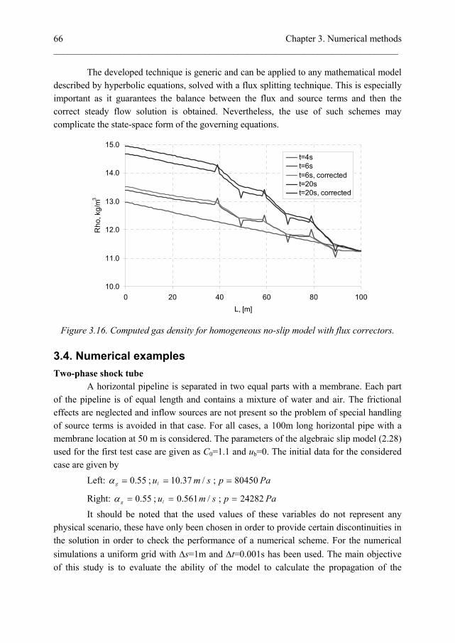
Chapter 3. Numerical methods _________________________________________________________________________ 66
The developed technique is generic and can be applied to any mathematical model described by hyperbolic equations, solved with a flux splitting technique. This is especially important as it guarantees the balance between the flux and source terms and then the correct steady flow solution is obtained. Nevertheless, the use of such schemes may complicate the state-space form of the governing equations.
10.0
11.0
12.0
13.0
14.0
15.0
0 20 40 60 80 100
L, [m]
Rh
o, k
g/m
3
t=4st=6st=6s, correctedt=20st=20s, corrected
Figure 3.16. Computed gas density for homogeneous no-slip model with flux correctors.
3.4. Numerical examples
Two-phase shock tube A horizontal pipeline is separated in two equal parts with a membrane. Each part of the pipeline is of equal length and contains a mixture of water and air. The frictional effects are neglected and inflow sources are not present so the problem of special handling of source terms is avoided in that case. For all cases, a 100m long horizontal pipe with a membrane location at 50 m is considered. The parameters of the algebraic slip model (2.28) used for the first test case are given as C0=1.1 and ub=0. The initial data for the considered case are given by
Left: 0.55g ; 10.37 /lu m s ; 80450p Pa
Right: 0.55g ; 0.561 /lu m s ; 24282p Pa
It should be noted that the used values of these variables do not represent any physical scenario, these have only been chosen in order to provide certain discontinuities in the solution in order to check the performance of a numerical scheme. For the numerical
simulations a uniform grid with s=1m and t=0.001s has been used. The main objective of this study is to evaluate the ability of the model to calculate the propagation of the

Chapter 3. Numerical methods _________________________________________________________________________
67
waves. Figure 3.17 shows the distribution the gas fraction at t=1.0s for different mesh refinements. The propagation of the liquid velocity is depicted in Figure 3.18. As can be seen, the obtained results are non-oscillatory, though the shocks are poorly resolved on a
standard mesh (s=1m). The use of the refined mesh (s=0.5m) improves shock resolution. Employing the standard grid with MinMod flux limiter gives a better approximation of the solution discontinuities, which is even better than for refined mesh case. This can further be improved by introducing superior flux limiters (SuperBee, van Leer), however for that particular case, the use other types of limiters than MinMod resulted into local oscillations near the contact discontinuity.
0.15
0.20
0.25
0.30
0.35
0.40
0.45
0.50
0.55
0.60
0 10 20 30 40 50 60 70 80 90 100
s, [m]
ag, [
-] 100cells
200cells
100cells+flux limiter
Figure 3.17. Simulated gas fraction at t=1s.
A similar test case has been used by [Fjelde and Karlsen, 2002] and [Evje and Fjelde, 2002] with a slightly different set of initial data. Gas volume fraction is quite accurately predicted by the proposed numerical method, though there is a slight mismatch in the determination of the shock position. That can be explained from the difference in formulation of the governing equations used to obtain the reference solution [Fjelde and Karlsen, 2002]. Without acceleration terms taken into account, the local speed of sound is defined by equation (2.50). Therefore the velocity of the flow is larger in the positive direction while it is slower in the direction opposite to the flow. This is only the case when the magnitude of the liquid velocity is comparable to the mixture speed of sound. Similar behaviour is observed for the liquid velocity in Figure 3.20. However, the velocity waves are induced with different magnitude. This problem arises from the fact that the reference

Chapter 3. Numerical methods _________________________________________________________________________ 68
simulations were performed with more complex slip model with a non-zero bubble drift velocity.
0.00
2.00
4.00
6.00
8.00
10.00
12.00
0 10 20 30 40 50 60 70 80 90 100
s, [m]
ul,
[m/s
]
100cells
200cells
100cells+flux limiter
Figure 3.18. Simulated liquid velocity at t=1s.
0.20
0.25
0.30
0.35
0.40
0.45
0.50
0.55
0.60
0 10 20 30 40 50 60 70 80 90 100
s, [m]
ag, [
-]
100cells+flux limiter
Reference
Figure 3.19. Simulated gas fraction at t=1s on a 100 cell grid using MinMod limiter
compared with reference solution (Fjelde and Karlsen, 2002)

Chapter 3. Numerical methods _________________________________________________________________________
69
0.00
2.00
4.00
6.00
8.00
10.00
12.00
0 10 20 30 40 50 60 70 80 90 100
s, [m]
ul,
[m/s
]
100cells+flux limiter
reference
Figure 3.20. Simulated liquid velocity at t=1s on a 100 cell grid using MinMod limiter
compared with reference solution (Fjelde and Karlsen, 2002). Pipe flow with inflow The second test case assesses the capabilities of the mathematical model to describe correctly the propagation of a convective wave. Proper simulation of the mass transport is a critical issue in many aspects of multiphase flow modelling and might be crucial for a multiphase soft-sensor. A problem of particular interest is related to the propagation of a holdup wave initiated by the rapid injection of gas or liquid phase from the reservoir. In addition, the developed numerical algorithm should be able to handle properly the generation and transport of dynamic waves and its propagation in both directions from the inflow point. Moreover, it is interesting to evaluate the ability of the scheme to handle frictional effects. The following test case is considered. Initially, the mixture of liquid and gas is flowing in a pipeline at steady conditions. After 60 seconds of production the gas is rapidly injected at s=50m located from the wellbore inlet (see Figure 3.21 for details). The value of the gas inflow source is 0.045 kg/s. As a result a liquid holdup wave is generated, which is propagates downstream the flow with the local velocity of the gas phase. The operating conditions used in this simulation correspond to a slug flow regime, and a simple drift flux model with constant C0 and zero bubble drift velocity ub is used. A standard set of boundary
conditions is used, in which the liquid holdup g and gas velocity ug are defined at the inlet of the simulation domain, and the gas density is prescribed at the outlet.

Chapter 3. Numerical methods _________________________________________________________________________ 70
The simulations are performed on a mesh composed of 100 grid blocks with a time step of 0.001 s. A standard first-order flux splitting algorithm is used. The source terms,
both g and Sfr were incorporated into a flux vector using the procedure defined in section 3.3. The friction factor is calculated according equation (2.18).
Table 3.3. Initial data for the test case 2
Quantity Value Pipe diameter, m 0.05 Pipe length, m 100
Liquid density, kg/m3 1000 Liquid viscosity, Pa.s 0.001
Gas reference density, kg/m3 11.9 Gas viscosity, Pa.s 1.82.10-5
Inflow holdup 0.4 Inflow gas velocity 3.1
Distribution coefficient C0 1.2 Bubble drift-velocity ub 0
Pipe roughness, m 0.0
l gF F
, /g kg s
g,t s
0.045
6050m
100m
Figure 3.21. Schematic representation of the test case 2.
The obtained results have been verified employing data obtained using the commercially available wellbore simulator OLGA [Bendiksen, 1991], using the same flow setup (Figure 3.21) to generate the reference data. Figure 3.22 shows the predicted gas velocity distribution at 61s and 62s, which represent the flow field after activation of the inflow source term. As expected, two waves travelling in the flow and counter flow direction are generated after the gas is injected in the simulation domain. The obtained results show that the developed wellbore simulator calculates flow dynamics,
corresponding to fast characteristics (2 and 3) with reasonable accuracy.

Chapter 3. Numerical methods _________________________________________________________________________
71
1
2
3
4
5
6
0 20 40 60 80 100
L, m
Ug
, m/s
OLGA, t=61s.
OLGA, t=62s.
1st order, t=61s.
1st order, t=62s.
Figure 3.22. Distribution of the gas velocity after gas injection at s=50m at 61s and 62 s.
The grid block size s=1m.
0.1
0.15
0.2
0.25
0.3
0.35
0.4
0.45
0 20 40 60 80 100
L, m
H, [
-]
OLGA, t=61s
OLGA, t=62s
OLGA, t=65s
OLGA, t=70s.
1st order, t=61s.
1st order, t=62s.
1st order, t=65s
1st order, t=70s
Figure 3.23. Distribution of the liquid fraction at t=61s, 62s, 65s and 70s after gas
injection at s=50m. The grid block size s=1m.

Chapter 3. Numerical methods _________________________________________________________________________ 72
The predicted liquid holdup is depicted in Figure 3.23 for several time instants up to a steady flow solution. The convective wave propagates with the gas velocity and is
characterized by the first eigenvalue 1=ug which gives an estimation of the holdup front position with the use of Figure 3.21. The provided results are in quite reasonable agreement with the reference solution. One can note that the use of a single velocity in a drift-flux formulation instead of the separate phase velocities in the two fluid model used by OLGA does not affect the dynamic response of the model related to convective transport. One can further note that the convective profiles are heavily smeared out due to numerical diffusion both for OLGA and for the developed wellbore simulator. Figure 3.24 represent the calculated liquid holdup for a case in which the pipeline is discretized with 50 grid blocks. In order to minimize the effect of numerical diffusion the scheme was modified to a second order scheme using MinMod flux limiter. The liquid holdup obtained using a high resolution scheme on the coarser mesh is as close to reference
solution as the results on a standard grid with s=1m. These results are promising from the soft-sensing perspective as it allows performing simulations with a reduced number of grid blocks maintaining at the same time good accuracy capabilities. The number of grid blocks can further be decreased by implementing more rigorous numerical algorithms and flux limiters. This in turn allows to reduce the size of the state vector and perform data assimilation faster.
0.1
0.15
0.2
0.25
0.3
0.35
0.4
0.45
0 20 40 60 80 100
L, m
H, [
-]
OLGA, t=61s
OLGA, t=62s
OLGA, t=65s
OLGA, t=70s.
MinMod, t=61s.
MinMod, t=62s.
MinMod, t=65s
MinMod, t=70s
Figure 3.24. Simulated liquid holdup on coarse mesh s=2m with MinMod flux limiter.

Chapter 3. Numerical methods _________________________________________________________________________
73
3.5. Summary
The numerical method for solving the two-phase gas liquid flow described by the drift-flux model has been formulated in this chapter. This method uses the splitting of the flux components according the model eigenvalues and explicitly accounts for the direction in which information is propagated. The performance of the flux splitting scheme may be improved by extending upwind schemes to high-resolution by introducing flux limiters. The difficulty associated with the structure of the equation, with source terms both in the continuity and momentum equations, causes incorrect representation of the steady-flow solution. In particular, the inflow source in the continuity equation generates oscillations in the density profile, which can not be suppressed using a refined mesh. The conservative properties of the numerical solution are maintained by introducing the integrated source as part of the flux term, which retains an exact balance with flux gradients. The developed schemes have been applied to find the solution of an inviscid two-phase shock tube, in which the importance of flux limiters has been demonstrated. In the second test case the performance of the developed wellbore model has been validated employing the well-established wellbore simulator OLGA. The developed numerical algorithm provides a realistic approximation of the reference solution.

Chapter 3. Numerical methods _________________________________________________________________________ 74

Chapter 4. A semi-implicit extended Kalman filter _________________________________________________________________________
75
4. A Semi-Implicit Extended Kalman Filter
4.1. Introduction
Complex industrial processes can often be described by sets of non-linear partial differential equations. Such equations, which are also known as first principle models, represent conservation of mass, momentum and energy within the system. Supplemented with constitutive relations and equations of state as well as appropriate boundary and initial conditions these describe the performance of the system in a continuous form. Such rigorous models can very accurately predict process behaviour, provided that adequate closure equations are available. There are many industrial processes in which the model parameters should be adjusted as these parameters are poorly known [Bloemen et al., 2004; Lorentzen et al., 2003]. In particular, reservoir engineering requires the knowledge of the properties of a porous medium. In this case the value of permeability and that of porosity of the medium determine the pressure and velocity distribution in the reservoir and, consequently, the accuracy of the prediction of the oilfield performance [Ertekin et al., 2001; Aziz, 1979]. However, due to high costs related to a direct measurement of the reservoir properties, combined with significant geological heterogeneity, there is an uncertainty in reservoir characterization. This, in turn, may result in poor performance of forward reservoir simulators and a corresponding decrease of oil production. This problem can be overcome by using data assimilation techniques (which are also referred to as history-matching or soft-sensing in petroleum engineering nomenclature) [Jansen et al., 2008]. In this approach, the poorly known unmeasured parameters are estimated by means of combining all the available observations with a dynamic model of the system. Whereas the forward problem consists of computing the distribution of pressures/velocities in the oilfield, the inverse problem consists of determining the unknown parameters from known (measured) dynamic variables. These measurements are usually quite sparse for hydrocarbon production systems, as the number of locations for sensors is very limited and available only in wells. The best estimate of the reservoir properties is obtained by minimizing the mismatch between the model prediction and the measurements. Here one can note two different approaches. Variational data assimilation, which is based on the minimization of a cost function within a certain time interval [Rommelse, 2010] and sequential history matching methods or filtering, in which the state of the system is updated every time instant new data become available. The latter updates reservoir properties in real-time, as new measurements are introduced in the assimilation process. For these purposes the sequential algorithms continuously update an initial estimate based on ongoing measurements.

Chapter 4. A semi-implicit extended Kalman filter _________________________________________________________________________ 76
One way to solve these sequential data assimilation problems is to use Kalman filtering [Kalman, 1960], which was originally developed for linear models. The Kalman filter is the optimal state estimator in the least square sense for linear models with both model and measurement error described by a Gaussian distribution. This algorithm has a predictor-corrector structure. First the state variables are calculated using a given process model, which are afterwards updated when the new set of measurements becomes available. The problem of model non-linearity can be solved using one of the available extensions of the original algorithm to non-linear models: The extended Kalman filter (EKF) [Jazwinski, 1970], the ensemble Kalman filter (EnKF) [Evensen, 1994], and the unscented Kalman filter (UKF) [Julier et al., 2000; Wan et al., 2000]. The EKF is the most straightforward extension to non-linear systems. It uses the linearization of the original non-linear process model around the previous estimate to update the error covariance matrix according to the standard linear Kalman filter equations. The usage of this linearization actually leads to the main shortcoming of the EKF approach; its application requires the computation of a Jacobian and hence the EKF may lead to poor estimates, which are far from optimal, in the case of strongly nonlinear dynamics [Evensen, 1992]. Although several special types of the EKF have been proposed [Pham et al., 1998; Verlaan and Heemink, 1979] in order to deal with high-order numerical models, little attention has been given to its performance from the point of model stability. In fact, the Kalman filter algorithm uses a space-state form of a process model, which is derived from the partial differential equations (PDE) model using appropriate numerical techniques [Crassidis and Junkins, 2004]. The use of the numerical methods implies spatial and temporal discretization and subsequent conversion of the original PDE into a system of algebraic equations [Ferziger and Peric, 2002]. Among the variety of time integration schemes used, one can distinguish between the implicit Euler scheme, which is unconditionally stable for the whole range of time steps, and the explicit one, which strongly defines the maximum value of the allowed time step. On the other hand, during recent years, more and more sensors are being deployed for monitoring pressure, temperature or flow rates in wellbores, with a very high data output frequency. It is important to incorporate the data as soon as these are available so that the reservoir model is always up-to-date and therefore the proper choice of time step, which is capable to perform stable simulations, is crucial for filter performance. The stability and convergence properties of EKF approach will definitely depend on the type of time integration, since the stability of the whole algorithm is related to the stability of the forward model. In this work attention is paid to the influence of the time integration scheme on the stability of both model propagation and error covariance matrix update during the forecast step of the EKF algorithm. Advantages and limitations of both implicit and explicit

Chapter 4. A semi-implicit extended Kalman filter _________________________________________________________________________
77
schemes are discussed. Moreover, a new type of EKF is proposed. With this new filter, the original non-linear state-space model, which is derived via the implicit time integration, is used for model integration in time (during the model forecast step for the Kalman filter approach), whereas the error covariance matrix is updated using the linearized model derived from the explicit Euler scheme. Using a series of generic test cases it will be shown that the proposed semi-implicit extended Kalman filter can partially diminish the time step limitation of the explicit Euler scheme, at the same time maintaining its superior capabilities in estimation accuracy. This chapter is organized as follows. First, the basic inverse problem considered here is presented. Then, issues are discussed related to the integration of the process model, in particular with respect to the explicit and implicit integration of this model. Then, the new semi-implicit EKF proposed here is outlined. This is followed by a discussion of the simulation based test cases to demonstrate the good properties of this algorithm. The chapter is summarized with the conclusions.
4.2. Formulation of the inverse problem
A hypothetical case in which the flow from a saturated rock formation to a single oil producing well is considered (Figure 4.1). For the sake of simplicity the oil properties are kept constant. The basic equations for the radial flow of a single phase slightly compressible fluid in a heterogeneous porous media are given by Darcy’s law [Dake, 1978]:
( )k r
w p
(4.1)
And the continuity equation:
( )
( ) 0wt
(4.2)
Where - porosity; p - pressure - density; k - permeability (which is a function of the radial coordinate for a heterogeneous reservoir), µ - oil viscosity and w - oil velocity. Oil is treated as a low-compressible fluid, which results in the following equation for the constant fluid compressibility
1
p
(4.3)
The closure for the problem is given by the following initial and boundary conditions
( , 0)res
p r p
( , )res res
p r t p (4.4)
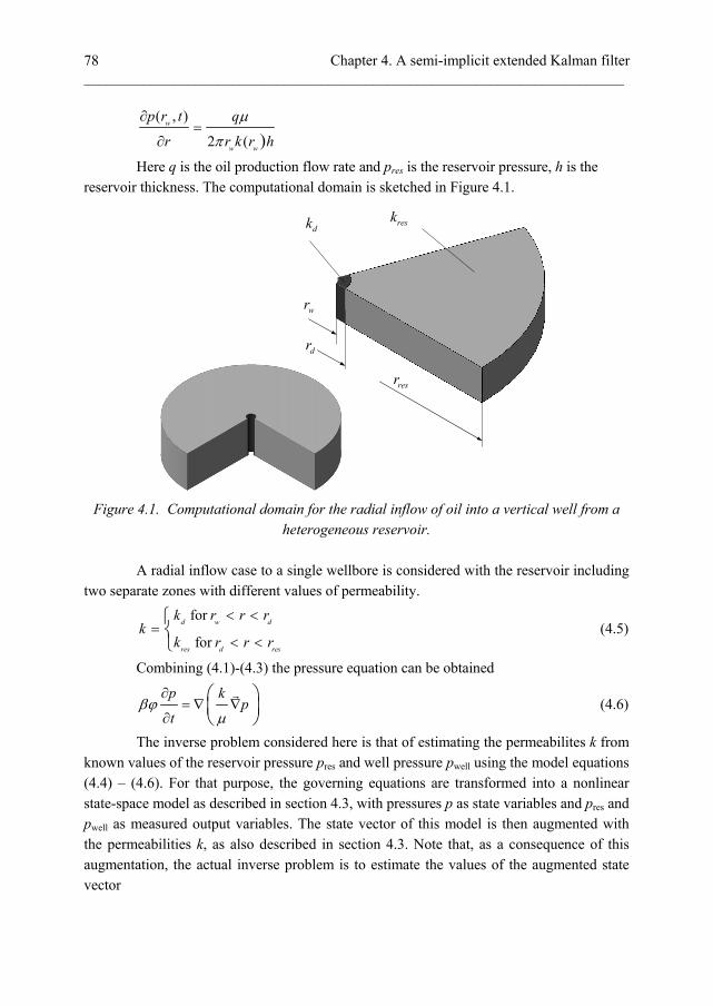
Chapter 4. A semi-implicit extended Kalman filter _________________________________________________________________________ 78
( , )
2 ( )w
w w
p r t q
r r k r h
Here q is the oil production flow rate and pres is the reservoir pressure, h is the reservoir thickness. The computational domain is sketched in Figure 4.1.
dk resk
wr
dr
resr
Figure 4.1. Computational domain for the radial inflow of oil into a vertical well from a
heterogeneous reservoir. A radial inflow case to a single wellbore is considered with the reservoir including two separate zones with different values of permeability.
for
for
d w d
res d res
k r r rk
k r r r
(4.5)
Combining (4.1)-(4.3) the pressure equation can be obtained
p k
pt
(4.6)
The inverse problem considered here is that of estimating the permeabilites k from known values of the reservoir pressure pres and well pressure pwell using the model equations (4.4) – (4.6). For that purpose, the governing equations are transformed into a nonlinear state-space model as described in section 4.3, with pressures p as state variables and pres and pwell as measured output variables. The state vector of this model is then augmented with the permeabilities k, as also described in section 4.3. Note that, as a consequence of this augmentation, the actual inverse problem is to estimate the values of the augmented state vector

Chapter 4. A semi-implicit extended Kalman filter _________________________________________________________________________
79
TX p k (4.7)
rather than only the permeabilities, from measurements of
[ ]T
well resy p p (4.8)
4.3. State-space form of model equations
To enable the usage of the PDE flow model equations form within an EKF approach, it is necessary to convert these into a state-space form. This model can be derived from a PDE formulation using different numerical techniques such as finite elements, finite differences or control volumes. All these methods involve spatial discretization of the simulation domain, which is divided into a finite number of non-overlapping control volumes. The given differential equation is then integrated over each control volume. In order to evaluate these integrals, the variation of state variables and model parameters between grid nodes is required. As a result, the discretization equation obtained in such manner expresses the conservation properties for the state variables for a finite control volume. The discretized simulation domain is given in Figure 4.2. The pressures are defined at discrete locations at the centers of the control volumes. Due to issues related to the numerical implementation permeabilities are needed at the interfaces of the control volumes. The interface value of permeability is obtained using the harmonic interpolation between adjacent grid nodes.
Figure 4.2. Discretized simulation domain with model states and parameters. The state variables are defined in the centers of grid blocks and the parameters at the interface.

Chapter 4. A semi-implicit extended Kalman filter _________________________________________________________________________ 80
With a process equation written as (4.6), generally two possibilities are available: one can either integrate equations in time using an explicit Euler scheme, or obtain the state-space form using an implicit scheme. Although both of these methods are of the same order of accuracy, the implicit scheme is unconditionally stable, meaning that there is no restriction on the value of time step used in the simulation. In contrast, the explicit Euler scheme provides a converging solution only if the time step is below a certain value obtained from a stability criterion, defined by the Courant number [Ferziger and Peric, 2002]. This makes this method inapplicable for highly transient problems; however, the explicit scheme is easier in numerical implementation. Omitting the derivation, the explicit scheme results, for the reservoir model considered here, in the following state-space form of the model equation
1
,k k k k
x f x d u (4.9)
For the implicit scheme this has the form
1 1,
k k k kg x d x u
(4.10)
Where x is a vector of pressures in the grid blocks,
1 2 ....T
Nx p p p (4.11)
d is a parameter vector of the permeabilities at the grid blocks interfaces
1.5 2.5 0.5....T
Nd k k k (4.12)
and u is a control input (i.e. boundary conditions). Subscripts k and k+1 denote quantities at an old and new time step. A comparison between equations (4.9) and (4.10) leads to the essential difference between the explicit and implicit Euler scheme: with the explicit scheme, the values of pressures and permeabilities form a nonlinear function on the old time level k, whereas for the implicit scheme these parameters are evaluated on the new time level k+1.
4.4. Data assimilation concepts
The extended Kalman filter One way to solve parameter estimation problems via the sequential data assimilation algorithm is by using the Kalman filter equations. The Kalman filter is a stochastic recursive estimator, which estimates the values of model states and unknown parameters by integrating available measurements in a mathematical model. Due to its straightforward numerical implementation and recursive nature, the Kalman filter algorithm is very adapted to real-time estimation. The Kalman filter was initially developed for linear dynamic systems. In case of non-linear systems, it can be modified by means of linearization around some reference

Chapter 4. A semi-implicit extended Kalman filter _________________________________________________________________________
81
value. In the EKF approach this linearization is performed around the most recent estimate. In case of nonlinear systems, the state vector x and the measurements vector y are respectively represented by the following relations:
1
,k k k k k
x f x d u v (4.13)
k k k k
y H x w (4.14)
Where f is a nonlinear operator. vk and wk are zero mean Gaussian white noise vectors, associated respectively with the model and measurements and characterized by variances Qk and Rk. Hk is the measurement matrix. The variables to be estimated are not always included in the state vector xk+1. In order to include parameters dk in the data assimilation process a simple and effective method is to augment the state vector with the parameters in the following way:
1
1
,k k k k k
k k
x f x d u v
d d
(4.15)
With an EKF the augmented state vector is estimated through the following two steps: 1) A time update or forecast step, which consists of the model forecast at tk+1 and corresponding update of the error covariance matrix associated with this prediction
1,f a a
k k k kx f x d u
(4.16)
,exp ,exp
1
f aug a aug T
k k k k kP P Q
(4.17)
Here, Φkaug,exp is the linearized state transition matrix derived in the Appendix A.
,exp/ /
0
aug
k
k
f x f d
I
(4.18)
2) A measurement update or correction step where the augmented state vector and the error covariance matrix are corrected using the measurements at tk+1:
1
1 1 1 1 1 1
f T f T
k k k k k k kK P H H P H R
(4.19)
1 1 1 1 1 1
a f f
k k k k k kX X K y H X
(4.20)
1 1 1 1
a f
k k k kP I K H P
(4.21)
Here I represents the identity matrix and K is the Kalman gain.
Implicit extended Kalman filtering The EKF approach described in the previous sub-section can directly be applied when using an explicit Euler integration scheme. Note that then, for obtaining stable and accurate EKF estimates, the time integration step for the model must be chosen sufficiently small and that this time step limitation may make the EKF computationally slow. To

Chapter 4. A semi-implicit extended Kalman filter _________________________________________________________________________ 82
overcome this problem, an implicit Euler scheme (4.10) can be used for solving the model equations as this allows for larger time steps without causing instability and, thereby, a faster EKF. When doing so, the EKF approach can be used directly with the notable exception that the time update step is now performed according to
1 1,f f a
k k k kg x d x u
(4.22)
, ,
1
f aug imp a aug imp T
k k k k kP P Q
(4.23)
with
1
,/ /
0
aug imp
k
k
g x g d
I
(4.24)
Equations (4.23) – (4.24) here follow straightforwardly from deriving a linearized model of equation (4.10) in standard form (i.e. with the state transition matrix (4.24) on the right side of the equality sign of the system equation) and applying the standard linear Kalman filter equations for propagation of the error covariance matrix through a linear system, assuming an additional white noise term vk with variance Qk. Contrary to the fully explicit Kalman filter, proposed in the previous section, the estimator based on a fully implicit model integration apparently does not exhibit stability problems for the model update step (4.22). However, the derivation of the tangent model in that case differs from the original Kalman filter algorithm, since the state-space form of the model equation (4.10) contains the non-linear function of model parameters on the new time level, while in the original Kalman filter approach it can be found on the old time level.
Semi-Implicit extended Kalman filtering As an alternative to the two above mentioned approaches a semi-implicit EKF is proposed. Here the implicit scheme is used to obtain the state-space form of the model equation, while the linearized state transition matrix is built based on the explicit time integration scheme. The semi-implicit EKF proposed here uses the same measurement update equations as the explicit and implicit EKF but uses a different set of time update equations:
1 1,f f a
k k k kg x d x u
(4.25)
,exp ,exp
1
f aug a aug T
k k k k kP P Q
(4.26)
Hence, its main characteristic is to solve the model equations in an implicit way while the new error covariance matrix is computed in an explicit manner. The flow chart of a semi-implicit extended Kalman filter is given in Figure 4.3.
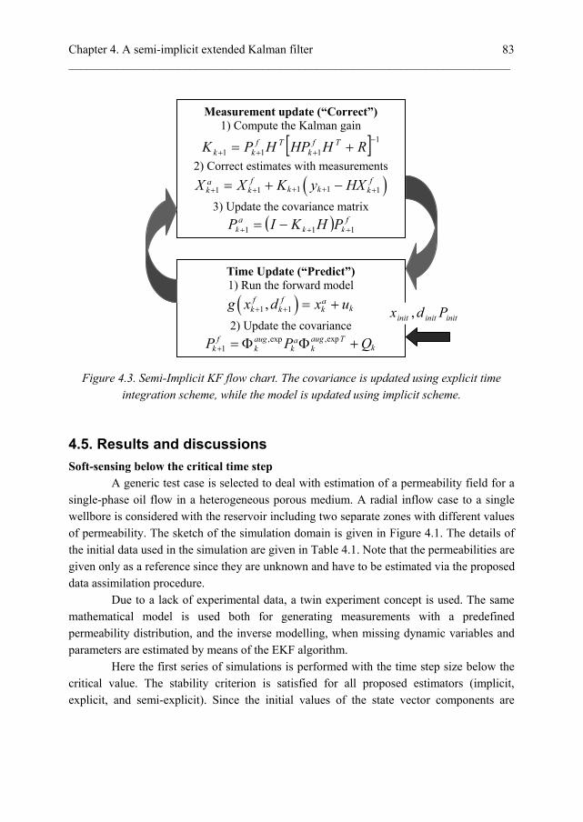
Chapter 4. A semi-implicit extended Kalman filter _________________________________________________________________________
83
Figure 4.3. Semi-Implicit KF flow chart. The covariance is updated using explicit time
integration scheme, while the model is updated using implicit scheme.
4.5. Results and discussions
Soft-sensing below the critical time step A generic test case is selected to deal with estimation of a permeability field for a single-phase oil flow in a heterogeneous porous medium. A radial inflow case to a single wellbore is considered with the reservoir including two separate zones with different values of permeability. The sketch of the simulation domain is given in Figure 4.1. The details of the initial data used in the simulation are given in Table 4.1. Note that the permeabilities are given only as a reference since they are unknown and have to be estimated via the proposed data assimilation procedure. Due to a lack of experimental data, a twin experiment concept is used. The same mathematical model is used both for generating measurements with a predefined permeability distribution, and the inverse modelling, when missing dynamic variables and parameters are estimated by means of the EKF algorithm. Here the first series of simulations is performed with the time step size below the critical value. The stability criterion is satisfied for all proposed estimators (implicit, explicit, and semi-explicit). Since the initial values of the state vector components are
Measurement update (“Correct”) 1) Compute the Kalman gain
1
111
RHHPHPK Tfk
Tfkk
2) Correct estimates with measurements
1 11 1 1f fa
k kk k kX X K y HX
3) Update the covariance matrix
fkk
ak PHKIP 111
Time Update (“Predict”) 1) Run the forward model
1 1,f f akk k kg x d x u
2) Update the covariance ,exp,exp
1aug Tf aug a
kk k k kP P Q
initinitinit Pdx ,

Chapter 4. A semi-implicit extended Kalman filter _________________________________________________________________________ 84
required, one should specify the initial pressure distribution and the guessed permeability field. The reservoir pressure was used to initiate the pressure part of the augmented state vector, while for the permeability the value in the near wellbore region, which is known from the core sampling [Dake, 1978], can be used. Therefore the initial augmented state vector can be written as
.... ....Taug
init res res well wellX p p k k (4.27)
Table 4.1. Initial data for numerical experiments
Quantity Value
Wellbore radius, rw 0.1 m
Damaged zone radius, rd 1.0 m
Reservoir radius 10.0 m
Oil density, 900 kg/m3
Oil viscosity, 0.01 Pa.s
Reservoir pressure, pres 10.106 Pa
Oil production rate, q 4.5.10-4 kg/(m.s)
Porosity, 0.2
Oil compressibility, 1.10-9 Pa-1
Reservoir permeability, kres 4.10-15 m2
Permeability near wellbore, kd 1.10-15 m2
Critical time step, tcr 3 s.
Figure 4.4 shows the estimated permeability field after 6000s of simulation. It is not quite accurate, though it is converging to a true value. The accuracy of estimating the permeability is strongly related to the propagation of the pressure in the reservoir, meaning that the position of the pressure front defines the area where the permeability can be accurately estimated. The final estimate of the permeability field (see Figure 4.5), which corresponds to a steady-state pressure distribution in the reservoir, is quite accurate for all proposed estimators. The difference between estimated and true permeability fields is caused by using a model error matrix Qk for propagation of the error covariance matrix Pf given by equations (4.17), (4.23) and (4.26). The use of the model error has a significant impact on the convergence properties of the all estimators used and the performance of the filter can be tuned by choosing a proper Qk matrix. It has been assumed for all the estimators used that the model error is related to the uncertainty in estimated model parameters. However, due to stability considerations, the elements of the Qk matrix were different for these three real-
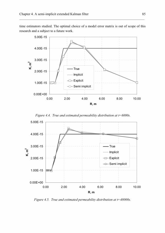
Chapter 4. A semi-implicit extended Kalman filter _________________________________________________________________________
85
time estimators studied. The optimal choice of a model error matrix is out of scope of this research and a subject to a future work.
0.00E+00
1.00E-15
2.00E-15
3.00E-15
4.00E-15
5.00E-15
0.00 2.00 4.00 6.00 8.00 10.00
R, m
K, m
2
True
Implicit
Explicit
Semi implicit
Figure 4.4. True and estimated permeability distribution at t=6000s.
0.00E+00
1.00E-15
2.00E-15
3.00E-15
4.00E-15
5.00E-15
0.00 2.00 4.00 6.00 8.00 10.00
R, m
K, m
2
True
Implicit
Explicit
Semi implicit
Figure 4.5. True and estimated permeability distribution at t=48000s.

Chapter 4. A semi-implicit extended Kalman filter _________________________________________________________________________ 86
Incorrect permeability initialization The second test case deals with the estimation of the permeability field where the parameter part of the augmented state vector is initialized with permeability values, which are different from the near-wellbore region. Here the initial value of the permeability is only 20% higher than in the vicinity of the wellbore. Results of the estimated permeability field, which correspond to the steady-state pressure distribution, are given in Figure 4.6.
-5.00E-15
0.00E+00
5.00E-15
1.00E-14
1.50E-14
0.00 2.00 4.00 6.00 8.00 10.00
R, m
K, m
2
True
Implicit
Explicit
Semi implicit
Figure 4.6. True and estimated permeability distribution at t=48000s. The initial
permeability field is different from near-wellbore value kd.
Application of the explicit and semi-implicit soft-sensors still provides a fair estimate of the permeability distribution. A soft-sensor based on the implicit scheme is diverging, resulting in unphysical permeability distribution. This problem may be caused by the implicit treatment of the estimated permeabilities which may not be processed properly in a high-gradient flow region in the vicinity of the wellbore. The figure clearly shows that the potential advantage of using a larger integration time step with the implicit EKF, and thereby obtaining a faster soft-sensor, is reduced by its sensitivity towards an error in the initial estimate. This sensitivity can be reduced by choosing a smaller integration time step (see Figure 4.7). The latter increases the computation time of the implicit EKF and thereby, diminishes its main advantage over its explicit counterpart.

Chapter 4. A semi-implicit extended Kalman filter _________________________________________________________________________
87
-5.00E-15
0.00E+00
5.00E-15
1.00E-14
1.50E-14
0.00 2.00 4.00 6.00 8.00 10.00
R, m
K, m
2
True
Implicit
Implicit (reduced time step)
Figure 4.7. Permeability distribution at t=48000 s. Implicit versus implicit with 5 times
reduced integration time step.
Soft-sensing above critical time step The final test case considered here aims to show that with the proposed semi-implicit EKF a larger integration time step can be obtained than with the explicit EKF while retaining the same estimation accuracy. The simulations were performed for the following values of the time step:
t=1.05tcr, t=4.0tcr and t=10.0tcr (see Figure 4.8-4.10) with tcr the critical time step
above which the explicit EKF becomes unstable (for that reason the results with this EKF are not depicted in these figures).
It can be seen that even up to an integration time step of t=4.0tcr the semi-
implicit EKF is still convergent and accurate estimates can be obtained. Figure 4.10, however, shows that the semi-implicit EKF also exhibits the shortcoming of the explicit scheme: for time steps considerably larger than the critical one, the semi-implicit estimator diverges. It is still unclear, to which extent the semi-implicit EKF can be used, as there are no exact mathematical criteria which describe its stability properties. The divergence of EKF type of estimator may be caused by the numerical errors induced by the linearization, which prevail for larger time steps. It has been observed that a certain choice of the error covariance matrix Qk may pull back the loss of stability of a semi-implicit approach.

Chapter 4. A semi-implicit extended Kalman filter _________________________________________________________________________ 88
0.00E+00
1.00E-15
2.00E-15
3.00E-15
4.00E-15
5.00E-15
0.00 2.00 4.00 6.00 8.00 10.00
R, m
K,m
2
True
Implicit
Semi implicit
Figure 4.8. Permeability field distribution at t=48000s. t=1.05tcr.
0.00E+00
1.00E-15
2.00E-15
3.00E-15
4.00E-15
5.00E-15
6.00E-15
0.00 2.00 4.00 6.00 8.00 10.00
R, m
K, m
2
True
Implicit
Semi implicit
Figure 4.9. Permeability field distribution at t=48000s. t=4tcr.

Chapter 4. A semi-implicit extended Kalman filter _________________________________________________________________________
89
0.00E+00
5.00E-15
1.00E-14
1.50E-14
2.00E-14
0.00 2.00 4.00 6.00 8.00 10.00
R, m
K, m
2
True
Implicit
Semi implicit
Figure 4.10. True and estimated permeability field distribution, t=10tcr.
4.6. Summary and conclusions
The question of stability of the real-time parameter estimation based on the extended Kalman filter has been discussed. Starting with a model of the single phase oil flow in a porous medium given in the PDE form three types of estimators were derived: implicit, explicit and semi-implicit. The fully implicit soft-sensor uses an implicit Euler scheme to obtain both the state-space form of the model equation and the Jacobian, which is used for the computation of the error covariance matrix. This scheme is unconditionally stable and no limitations on the time step size are imposed to update the model in time. Via a series of test cases, it has been shown that the choice of initial conditions (the initial permeability distribution) is crucial to provide satisfactory performance of a fully-implicit soft-sensor: when chosen too far from real permeability field, the filter diverges. For the cases where good initial conditions are not available, the problem of divergence may be overcome by imposing small values of the time step. This, however, diminishes the main advantage of the implicit approach – the capability to run the simulations with large time steps. In contrast, the fully explicit soft-sensor provides the state-space form of the process such that the EKF algorithm can be directly implemented. However, due to the fact that the explicit Euler scheme is both used for model and covariance update, the selected

Chapter 4. A semi-implicit extended Kalman filter _________________________________________________________________________ 90
time step should not exceed the value prescribed by the stability criterion. However, this estimator seems to provide quite reliable and accurate results regardless the initial guess of the model states and parameters. The semi-implicit soft-sensor, which is proposed in this chapter, combines the two above mentioned algorithms to a certain extent, trying to eliminate their disadvantages and reinforce the strong parts. In this approach the implicit Euler scheme is used for the model integration and derivation of the state-space model, which is unconditionally stable, while the linearized model matrix, obtained via the explicit Euler scheme, is used for covariance propagation. The latter allows the use of the original concept of the EKF and therefore the calculation of better estimates of dynamic variables and unmeasured parameters. Via simulation based test cases it has been demonstrated that this new estimator is slightly affected by initial conditions and can be used for an extended range of time steps.
Chapter 5. Inverse modelling of the inflow distribution for the liquid/gas flow in horizontal pipelines
91
5. Inverse Modelling of the Inflow Distribution for the Liquid/Gas Flow in Horizontal Pipelines
5.1. Introduction
Transmission and reflection of dynamic waves in pipelines filled with fluids are governed by the elastic properties of the propagation medium. The acoustic properties are influenced by changes in fluid composition, fluid density and pipeline geometry or its material properties. It seems, therefore, promising to use the transient information from these waves in order to analyze the flow structure. Rapid pressure transients in wells and flowlines may be caused by quickly operated inflow control valves, flow rate variations, flow regime instabilities, leakages or induced by the reservoir dynamics, such as gas or water breakthrough phenomena. In particular, rapid increase of gas or liquid phase in a given location of the wellbore is followed by an instantaneous increase in pressure due to the flow acceleration. The generated pressure pulse will propagate with a speed of sound in the directions upstream and downstream the inflow point and can be detected with the measurement instruments placed along the well. Several attempts have been made over the last decade to use propagation of acoustic waves in order to perform flow analysis both for single and multiphase flows. The investigations were performed for various applications of pipeline monitoring including leak detection and flow metering problems. A methodology to detect the pipe break in water transport pipelines was proposed by Misiunas et al., (2005). The pipe break produces a pressure wave, which travels forward and reflects from the boundary of a pipe. The measurements of the pressure signal at one location along the pipeline were used to determine both position and the magnitude of the leak. Wang et al., (2002) processed transient pressure signal with a Fourier analysis to detect and identify leakages in water pipelines. The leak detection technique is based on the principle of the difference in Fourier components for leak damping, where the magnitude of the damping indicates the size of the leak, while different dumping ratios of the various Fourier components specify its location. A leak detector combined with a gas-composition tracking system, based on a simple transient multiphase flow model, is presented by Erickson and Twaite, (1996). The monitoring system predicts the outflow rate and compares it to a measured value. Scott and Yi, (1998) presented a leak detection technique which is based on standard production data, namely, inlet and outlet pressure and outlet flow rate. The method accounts for the momentum balance and detects changes in pipeline frictional losses caused by a leakage. The application of the flow transient analysis for production monitoring purposes has multiple examples. A pressure pulse method introduced by Gundmundsson, (1999) is based on the generation of pressure waves by quickly closing and opening a valve installed
Chapter 5. Inverse modelling of the inflow distribution for the liquid/gas flow in horizontal pipelines 92
on a flow line. This pulse is registered at two pressure transducers installed upstream the valve. The relevant flow parameters are then extracted from the sensor readings in order to calculate the flow rates. The multiphase flow meter introduced by Piantanida et al., (1998) uses an acoustic sensor, which records noise generated by flow over a choke valve. The developed instrument employs digital signal processing algorithm and neural network models in order to extract multiphase flow rates from the acoustic signal. All the pressure signal processing techniques combine continuous monitoring of measured parameters and rigorous mathematical modelling to a certain extent. A typical set of measurements includes flow rate meters and pressure sensors installed in one or several locations in the pipeline. Although the mathematical techniques used for transient pressure analysis considered were initially developed and implemented to deal with a single phase water flow, their benefits in usage within oil and gas industry are apparent. Within a smart wells approach it is common practice to perform a very large investment in wellbore instrumentation. Consequently, since more measurements can be assimilated to process the transient flow signal, one can expect the improved performance of the equipment installed. With the increasing usage of multiphase flow meters worldwide, petroleum companies are looking for robust methods, which offer sufficiently accurate solutions for production optimization and provide a balance between costs and performance capabilities. For long horizontal pipelines with multiple inflow points the following aspects are important with respect to flow date processing. First, once should measure or estimate the multiphase flow rates in real-time during the transient flow in horizontal wells, which is caused by various production instabilities. Secondly, for the case where inflow of liquid or gas phase from a reservoir takes place, it is required to identify the amount of fluid entering the well and specify its composition in real time. The improvement in multiphase flow metering can be achieved only if the parameters relevant for the flow estimation are included explicitly in a physical model of multiphase wellbore flow. In particular, proper description of wave propagation phenomena may be used together with measurement data. The quantities of interest may then be estimated using any data assimilation technique. For the multiphase flow allocation the following issues are important. First, the sensitivity of the method (which corresponds to the inflow, found via a suitable algorithm) as well as the time required for the algorithm to do a proper inversion need to be specified. Secondly, the accuracy of the technique is important, which refers to its ability to estimate the relevant flow parameters, while the input measurements are corrupted with a certain measurement noise. Finally, one should define a necessary and sufficient set of measurements which provides a reasonable balance between operational costs and predictive capabilities of the method. The goal of this chapter is to perform a feasibility study which assesses the performance and possibilities of combined usage of flow models with data assimilation techniques. This chapter is organized as follows. First the general analysis of the pressure

Chapter 5. Inverse modelling of the inflow distribution for the liquid/gas flow in horizontal pipelines
93
pulse generated due to multiphase inflow is performed. Secondly, a simplified setup for flow rate estimation is considered. The next section deals with the description of the used soft-sensing algorithm. Finally, the inflow detection procedure is considered, which is verified using an artificial set of measurement data. At the end of the chapter, the conclusions are given.
5.2. Qualitative analysis of pressure transients
Dynamic wave propagation in horizontal wells A dynamic wellbore flow simulation can be accurately performed with a drift-flux model, introduced in Chapter 2. In order to test the performance of the flow estimator, in case of rapid gas or liquid inflow variation, a set of artificial measurement data is used. These data are generated using either the same mathematical model or using another wellbore simulator with a similar mathematical model and same estimation setup. Such approach can guarantee that the proposed estimation algorithm is capable to perform the inversion properly, disregarding the type of mathematical model used in the simulations. Despite the variety of application of pressure transient interpretation for flow assurance, the majority of studies are related to single phase flows. In multiphase flow the transient pressure signal, which is accompanied by a variation in fluid composition, behaves in a different way. Therefore, first preliminary simulations are performed in order to get a qualitative description of transient pressure analysis and evaluate the possibilities for multiphase metering. Here the main question addressed is if the information, which is transported with a generated pressure wave, is sufficient for the estimation of the multiphase rates. It is also important to specify other applications which might be useful from the analysis of available data. For the purpose of qualitative pressure analysis, the following test case is considered. The simulations are performed for flow of a gas-liquid mixture in a 1000m horizontal pipeline of 0.05m diameter. For simplicity, the gas and liquid are assumed to flow with the same velocity. After simulation of several seconds of the flow, sufficient for obtaining steady-state distribution of the flow parameters, the inflow source is introduced. This source is a single phase gas (test case 1) or a single phase liquid (test case 2). The gas density is equal to 100 kg/m3 and the liquid density is 1000kg/m3. The inflow gas and liquid flow rates are equal to 5 kg/s and 0.5 kg/s respectively. These values will result in the same increase in the local velocity (Figure 5.3). The computational setup of these test cases is depicted in Figure 5.1 and 5.2. The inflow source is located approximately in the middle of the simulation domain, so it takes about equal time for a generated pressure pulse to travel in both upstream and downstream directions.

Chapter 5. Inverse modelling of the inflow distribution for the liquid/gas flow in horizontal pipelines 94
l gF F
0.5 kg/s
Gas
l gF F
5 kg/sLiquid
Figure 5.1. Forward simulation of
pressure wave generated by gas inflow. Figure 5.2. Forward simulation of pressure
wave generated by liquid inflow. Due to the inflow generated, pressure wave propagates with a velocity equal to the mixture speed of sound. The simulated pressure distribution for two time instants is depicted in Figure 5.4. It should be noted that due to the direct relation between gas density and pressure used in the simulations (equation 2.20), the plot obtained can be easily rescaled for a different density of the gas phase. It can be observed from the figures, that the different inflow scenarios, i.e. pure liquid and pure gas, produce similar pressure and velocity responses. The obtained result is not surprising as there is no direct influence of the source composition on the propagation of the pressure/velocity waves.
0.00
1.00
2.00
3.00
4.00
5.00
6.00
7.00
0 200 400 600 800 1000
L, m
u, m
/s
reference
oil inflow, t1
gas inflow, t1
Figure 5.3. Simulated flow velocity plotted at t=60.2 s time. The inflow source activated at
t=60 s. Both cases with liquid and gas inflow are considered. The velocity response is similar for both sources.

Chapter 5. Inverse modelling of the inflow distribution for the liquid/gas flow in horizontal pipelines
95
1.05E+07
1.10E+07
1.15E+07
1.20E+07
1.25E+07
1.30E+07
1.35E+07
0 200 400 600 800 1000
L, m
P, P
a
reference
oil inflow, t1
gas inflow, t1
oil inflow, t2
gas inflow, t2
Figure 5.4. Simulated pressure. The pressure (density) waves are plotted at two time
instants with time instants of 60.2s. and 61s. after the injection.
As it has been pointed out in Chapter 2, the propagation of the dynamic waves is not affected by the kinematic ones. In other words, the speed of sound which governs the propagation of pressure and velocity pulses, is defined by the properties of the undisturbed medium, as it is a function of liquid holdup mainly, which develops much slower than pressure and velocity. For the considered case, the mixture speed of sound is ~230 m/s, while the holdup wave travel with an average velocity of 4 m/s (see Figure 5.3). Once the pressure wave is generated it rapidly moves away from the inflow point, while the holdup moves only a small distance downstream the inflow location. At the time instant t2=61s, the pressure wave is approximately 230 meters away from the inflow point though the composition change due to inflow occurs only at a 4 meters length interval. The relevant information regarding inflow composition can only be extracted if the pressure wave is transmitted over a flow region which is covered by the convective wave, which is not possible considering the same source which produces the pressure pulse. Here the solution may be in inducing additional pulsations in the vicinity of the inflow source, by means of manipulating the flow with internally installed valves or actuators. The disadvantage of this is again related to a relatively high discrepancy between mixture speed of sound and flow velocity: since a pressure signal is rapidly propagating in the wellbore, it is expected to use a high number of pressure sensors over a short wellbore interval, which should be placed with very high spatial density. That might not be possible from the

Chapter 5. Inverse modelling of the inflow distribution for the liquid/gas flow in horizontal pipelines 96
economic point of view. The proposed approach is illustrated in Figure 5.5.
0
0.1
0.2
0.3
0.4
0.5
0.6
0.7
0.8
0 20 40 60 80 100
L, [m]
H, [
-]
g
Generate flow disturbance upstream the inflow point (i.e valve)
pressure sensor
Figure 5.5. Measurements layout for inflow holdup estimation.
However, a transient pressure signal may still be useful, as it contains the information relevant to the flow velocity. With any disturbance generated in the pipeline, the dynamic phenomena related to fast waves occur on two time scales. First, one can consider acceleration effects due to sudden variation in flow velocity. By using a proper correlation for a pressure increase due to acceleration (i.e. the Joukowski-water hammer equation), one can in principle estimate the velocity component. However, this information is available only on a short term time scale, as the dynamic effects are rapidly diminished by frictional attenuation. The rate of attenuation is dictated by the roughness of the pipeline, its geometry and flow velocity, and flow composition. With the given correlation for frictional pressure drop and the mixture velocity obtained from processing of a dynamic pressure pulse, one can estimate the flow composition. One should note however, that the estimation of the liquid fraction is performed in a “semi-steady” state regime, as it corresponds to a frictional pressure distribution in wellbore. Therefore one can note two steps in the estimation procedure. First the fully transient information is processed in order to extract the data relevant to the flow velocity. The information about the magnitude of the inflow source is then transferred to the operator in the time scale of seconds. Secondly, these data are used to provide an estimation of the liquid holdup using frictional effects. The latter may be performed on any time scale which is relevant to a user. One can also conclude that the transient information is more useful on the short-term time (and length) scale, and therefore the transient effects should be considered locally, for example as an integrated part of wellbore instrumentation. On the other hand, the steady frictional effects are acting on a long length scale and are more suitable for usage in management of a production system.

Chapter 5. Inverse modelling of the inflow distribution for the liquid/gas flow in horizontal pipelines
97
Measurement of the mixture speed of sound The liquid holdup can be estimated directly by means of incorporating its values into the state vector. Alternatively, one can estimate the liquid fraction implicitly, by accounting its influence on the propagation of speed of sound. This is reasonable, since the speed of sound defines the dynamics of pressure wave propagation, which is available via measurements. In general case speed of sound also depends on flow regime and details of the droplet and bubble size. For the case of homogeneous flow equation (2.50) can be modified as follows
2
(1 ) (1 )
g
ph g
g l
u cH H H
(5.1)
As the convective acceleration is neglected, the obtained mixture speed of sound is a function only of the local liquid holdup H, provided that the variation of gas and liquid density is insignificant. Therefore proper interpretation of the pressure pulses, induced on the domain with holdup value of H together with estimation of velocity as discussed earlier would result in the estimated values of multiphase rates. However, solving equation (5.1) for liquid holdup will provide two different solutions. This is illustrated in Figure 5.6. This graph may be more complicated if one accounts for the heat transfer phenomena.
100
200
300
400
500
600
700
0 0.2 0.4 0.6 0.8 1
Liquid Holdup H, [-]
Mix
ture
sp
ee
d o
f s
ou
nd
, m/s
p=100 bar
measured
Figure 5.6. Mixture speed of sound defined using equation 5.1 and possible inverse
solution. The possibility of multiple solutions is demonstrated.
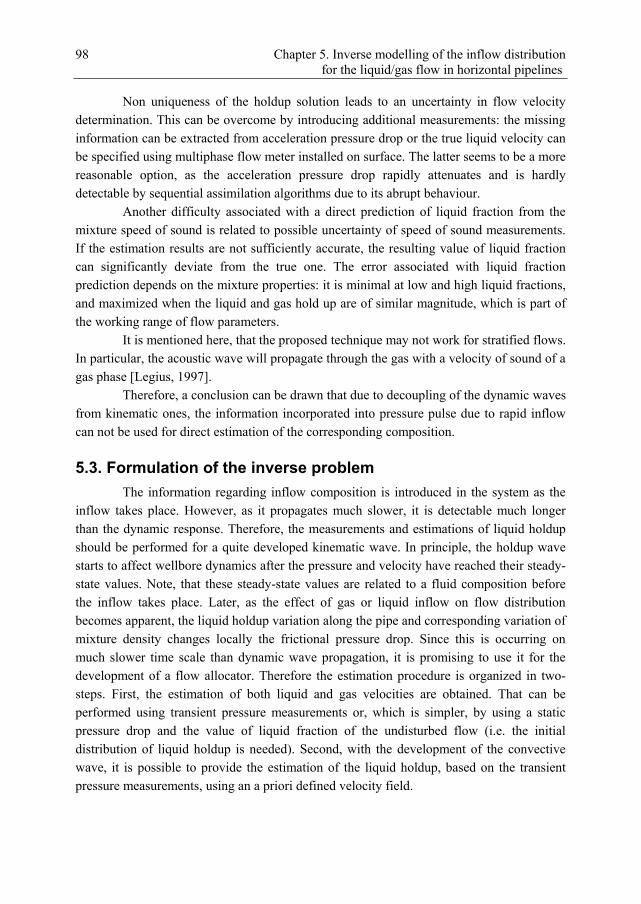
Chapter 5. Inverse modelling of the inflow distribution for the liquid/gas flow in horizontal pipelines 98
Non uniqueness of the holdup solution leads to an uncertainty in flow velocity determination. This can be overcome by introducing additional measurements: the missing information can be extracted from acceleration pressure drop or the true liquid velocity can be specified using multiphase flow meter installed on surface. The latter seems to be a more reasonable option, as the acceleration pressure drop rapidly attenuates and is hardly detectable by sequential assimilation algorithms due to its abrupt behaviour. Another difficulty associated with a direct prediction of liquid fraction from the mixture speed of sound is related to possible uncertainty of speed of sound measurements. If the estimation results are not sufficiently accurate, the resulting value of liquid fraction can significantly deviate from the true one. The error associated with liquid fraction prediction depends on the mixture properties: it is minimal at low and high liquid fractions, and maximized when the liquid and gas hold up are of similar magnitude, which is part of the working range of flow parameters. It is mentioned here, that the proposed technique may not work for stratified flows. In particular, the acoustic wave will propagate through the gas with a velocity of sound of a gas phase [Legius, 1997]. Therefore, a conclusion can be drawn that due to decoupling of the dynamic waves from kinematic ones, the information incorporated into pressure pulse due to rapid inflow can not be used for direct estimation of the corresponding composition.
5.3. Formulation of the inverse problem
The information regarding inflow composition is introduced in the system as the inflow takes place. However, as it propagates much slower, it is detectable much longer than the dynamic response. Therefore, the measurements and estimations of liquid holdup should be performed for a quite developed kinematic wave. In principle, the holdup wave starts to affect wellbore dynamics after the pressure and velocity have reached their steady-state values. Note, that these steady-state values are related to a fluid composition before the inflow takes place. Later, as the effect of gas or liquid inflow on flow distribution becomes apparent, the liquid holdup variation along the pipe and corresponding variation of mixture density changes locally the frictional pressure drop. Since this is occurring on much slower time scale than dynamic wave propagation, it is promising to use it for the development of a flow allocator. Therefore the estimation procedure is organized in two-steps. First, the estimation of both liquid and gas velocities are obtained. That can be performed using transient pressure measurements or, which is simpler, by using a static pressure drop and the value of liquid fraction of the undisturbed flow (i.e. the initial distribution of liquid holdup is needed). Second, with the development of the convective wave, it is possible to provide the estimation of the liquid holdup, based on the transient pressure measurements, using an a priori defined velocity field.

Chapter 5. Inverse modelling of the inflow distribution for the liquid/gas flow in horizontal pipelines
99
The estimation of the inflow profile with the proposed semi-transient technique is possible under the following assumptions: 1) u2ph> ug,ul , which guaranties that the dynamic waves do not affect the propagation of the convective waves. 2) The inflow is instantaneous, which allows to obtain the initial estimation of the velocity field.
No pressure wave (NPW) dynamic model For the proposed simplified setup a comprehensive wellbore simulation is not required. Although one can directly use the proposed simulator based on the drift-flux model, the outlined simplification may be used. In particular, since the pressure and velocity transients are not important, the corresponding transients can be left out from the
computation procedure. That is possible by setting the corresponding eigenvalues 2 and 3
to infinity. The continuity equations corresponding to the so called no-pressure-wave model (NPW) are the same as for a standard drift flux model and given by
l l l l l
Vl
u
t s
(5.2)
g g g g g
Vg
u
t s
(5.3)
The momentum equation for the oil-gas mixture is formulated in a steady form
fr
pS
s
(5.4)
The model is complemented by algebraic slip law, where the gas velocity is given by
0 ( )g l g bl gu C u u u (5.5)
The frictional loss Sfr is calculated using relation (2.10). Considering the fact that the dynamic waves are decoupled from the kinematic waves and the holdup wave propagates only in the direction coinciding with the flow, the numerical strategies in this case are much simpler. In particular, it is possible to use implicit central scheme for pressure and velocity and explicit upwind scheme for the hyperbolic equation which governs the propagation of holdup wave in the system. For the discretization of the simulation domain a staggered grid approach has been used, meaning that a different grid for the continuity and momentum equation has been employed. The flux related variables are defined at the interface of a grid block and others are specified at the centers of grid blocks (Figure 5.7). Pressure and liquid fraction are defined in the centers of a gridblock, while the velocity (liquid or gas) are calculated at the grid interfaces.

Chapter 5. Inverse modelling of the inflow distribution for the liquid/gas flow in horizontal pipelines 100
i i+1/2 i+1i-1/2i-1
i+1/2i-1/2
i-1 i i+1
Continuityequation
Momentumequation
Figure 5.7. Staggered grid and definition of the state-variables. Momentum and continuity equations are discretized on different grids.
The mass conservation equations are formulated for the gridblock with boundaries [si-1/2, si+1/2]. Therefore, the discrete liquid continuity equation is given by
1
1/ 2 1/ 2
n n n nn nl l l ll i l i i i
l l Vl i
u u
t s
(5.6)
Where the interface values of the fluxes are evaluated using a simple upwind scheme of the first order.
1/ 2 1/ 2
1/ 2
1 1/ 2 1/ 2
0
0
n n nl i l i l i
n nl l i n n n
l i l i l i
u if uu
u if u
(5.7)
The momentum conservation equation is discretized on the displaced grid [si, si+1] with centers located on the interfaces
1 1 1
1 1 / 2
n n n
i i fr ip p S s
(5.8)
The total number of variables for that formulation is composed of N pressures, N holdups and N-1 velocities with N number of grid blocks. Therefore the coupled solver may require substantial amount of mathematical operations. The solution however may be simplified dramatically, if one instead of solving all the equations simultaneously chose for a segregated approach. With a given holdup one can calculate the velocity from the continuity equation, and then update the holdup distribution, which is used in turn to calculate the pressure gradient implicitly from eq. 5.8. That is feasible also due to the physics of the process. Once the velocity field is established due to inflow it is hardly influenced by the propagating holdup wave. The development of a robust segregated solver also requires the assumption of a weak relation between gas density and pressure. Gas density variations may be computed iteratively using the obtained pressure field. The explicit treatment of the convective terms in the continuity equations is driven by the following facts. First, it allows to attach flux limiters (Chapter 3). Secondly, though

Chapter 5. Inverse modelling of the inflow distribution for the liquid/gas flow in horizontal pipelines
101
the solution can be obtained with a reduced number of time steps, this is not always needed from the point of availability of measurements. Secondly, as the implicit schemes are generally more diffusive, the quality of estimation might be reduced.
Extended Kalman filtering One way to solve estimation problems via the sequential data assimilation algorithm is by using the Kalman filter equations. The Kalman filter is a stochastic recursive estimator, which estimates the values of model states and unknown input by combining measurement data in a mathematical model in real-time. Due to its straightforward numerical implementation and recursive nature, the Kalman filter algorithm is very well adapted to online model calibration. Kalman filtering was initially developed for linear dynamic systems. Although the ensemble Kalman filter (EnKF) is widely used nowadays to handle model non-linearity, in this work the extended Kalman filter (EKF) is implemented [Jazwinski, 1970]. The difference between these two algorithms is in the way the error covariance matrix is calculated. It is represented by the ensemble of possible model realization in the EnKF algorithm, and the EKF calculates the approximation of the covariance matrix using a linearized process model. For the estimator developed in this chapter the EKF demonstrated good performance, which indicates that the error induced due to the linearization is minor. With respect to computation time, the performance of the EKF depends on the number of states Nst (the size of the augmented state vector X), while the EnKF performance is based on the chosen ensemble size denoted here as Nens. More specific, the EKF computation time is typically of the order of Nst model simulations, and the EnKF computation time is approximately of the order of Nens model simulations. Therefore, the size of the ensemble is a crucial issue with the use of the EnKF. Based on the experience of data assimilation for large-scale atmospheric models [Houtekamer and Mitchel, 1998], at least 100 ensemble members should be chosen for the ensemble Kalman filtering. The optimal size of the ensemble for inflow estimation is, however, not known and it is a subject for future research. As a result, the EKF is normally faster than the EnKF for low order systems (Nst<100), which is the case for the majority of the soft-sensing applications for wellbore flow. The discrete equations obtained with the use of NPW model can be reformulated in the following state-space notation.
1
,k k k
x f x u (5.9)
Where x is a vector of pressures and liquid holdups in the grid blocks,
1 2 1 2.... ....T
N l l l Nx p p p (5.10)
u is an input vector which includes boundary conditions and values of the velocity at the interfaces. Although it is usual to consider the velocity as one of the components of the

Chapter 5. Inverse modelling of the inflow distribution for the liquid/gas flow in horizontal pipelines 102
state vector, it is more convenient to reformulate it in this case differently and treat the velocity as the model input. This is governed by the fact, that with the use of NPW model, the velocity field is calculated just in the beginning of the simulation and kept static during all the time steps.
is the input vector which represents the inflow from reservoir to wellbore, and
for two phase gas liquid flow it is represented by the two following components l g].
The model equation (5.9) formulated with the added model noise and measurement equation which relates observed states and available measurements is given by
1,
k k k k kx f x u v
(5.11)
k k k k
y H x w (5.12)
Where f is a nonlinear operator. vk and wk are zero mean Gaussian white noise vectors, associated respectively with the model and with measurements and characterized by variances Qk and Rk. Hk is the measurement matrix which relates the states with the measurements available. Since the variables to be estimated, i.e. the components of the model input, are not included in the state vector x, it should be modified using the similar approach as in the
previous chapter. The state vector is then augmented with the inflow and the augmented
state vector X=[x ]T is further used within the data assimilation framework
1
1
,k k k k k
k k
x f x u v
(5.13)
With an EKF the augmented state vector is estimated through the two steps, which are outlined in Chapter 4 (eqs. (4.16)-(4.21)). The use of the explicit time integration scheme becomes apparent, as it allows to use the traditional Kalman filter equation without limitation (only the time step limitation does exist). The attractive idea of using a semi-implicit KF, which was introduced in a previous chapter, for that particular problem may fail as there is a substantial model difference between explicit and implicit schemes, which requires fine tuning of model error matrix.
5.4. Results and discussions
Test Case 1. Holdup estimation under measurement error To examine and evaluate the proposed estimation methodology for multiphase inflow estimation, the inflow in a segment of a horizontal well is considered. The simulations are performed in a 100m well of 0.05m diameter where the simulation domain is represented by a uniform grid of 50 internal gridblocks. The parameters of interest are the inflow sources, which are instantaneously introduced in the simulation domain. These

Chapter 5. Inverse modelling of the inflow distribution for the liquid/gas flow in horizontal pipelines
103
sources, result in a change in the liquid holdup and consequently in the pressure gradient. The purpose of this study is to estimate the obtained holdup field in real-time using various estimation scenarios. The input to the estimation problem is defined by the pressure measurements. For the base simulation case, the number of pressure sensors installed is equal to the number of grid blocks. The sampling time was constant for most test cases and equal to 0.1s, unless otherwise stated. The first test considered deals with the estimation of the holdup distribution in a horizontal well where only gas enter the wellbore in the radial direction. Two inflow scenarios are considered. First a single source located close to the wellbore inflow point is estimated using the proposed algorithm. Secondly, the method is extended to a more complex case with multiple gas inflow points. The simulation layouts are sketched in Figure 5.8 and 5.9.
ginu
1g
12005
0.02
1x
inH
ginu
g
12005
0.02
1xinH
2x3x
Figure 5.8. Computational setup for
estimation of single gas inflow. Figure 5.9. Computational setup for
estimation of multiple gas inflow. The locations of the inflow points and other data relevant to the simulation are given in table 5.1. The speed of sound of the two phase mixture, which corresponds to the initial data, is approximately equal to 90 m/s which is considerably higher than the gas velocity. Such value of the mixture acoustic velocity guaranties that the transients relevant to dynamic waves occur on a much faster time scale, which makes the use of the NPW model feasible. The results of the simulations for the single inflow source are depicted in Figure 5.10. It is obvious that in the absence of measurement error the proposed algorithm is very well capable to estimate the propagation of the liquid holdup. The influence of the measurement error on the quality of the estimates is illustrated on the next figure, where the input pressure measurements are corrupted with a certain noise. The standard deviation of the pressure measurements errors was only 50 Pa (for an outlet pressure of 106 Pa). Such low measurement noise for the pressure leads to a standard deviation in the liquid fraction in the order of 0.01.

Chapter 5. Inverse modelling of the inflow distribution for the liquid/gas flow in horizontal pipelines 104
Table 5.1. Initial data for the numerical experiments
Quantity Values for case 1 Values for case 2 Pipe diameter, m 0.05 Pipe length, m 100
Liquid density, kg/m3 1000 Liquid viscosity, Pa.s 0.001
Gas reference density, kg/m3 11.93 Gas viscosity, Pa.s 1.82.10-5
Inflow holdup H, [-] 0.8 Inflow gas velocity ug, m/s 2.1876
Outlet pressure, Pa 106 Absolute roughness, m 0
Distribution parameter, [-] 1.2 Bubble drift velocity, m/s 0
x1, m 7 7 x2, m - 39 x3, m - 69
0.30
0.40
0.50
0.60
0.70
0.80
0.90
1.00
0 20 40 60 80 100
L, m
H, [
-]
True, t=10s
Estimated, t=10s
True, t=20s
Estimated, t=20s
0.30
0.40
0.50
0.60
0.70
0.80
0.90
1.00
0 20 40 60 80 100
L, m
H, [
-]
True, t=10s
Estimated, t=10s
True, t=20s
Estimated, t=20s
Figure 5.10. True and estimated liquid
holdup with noise free data. Figure 5.11. True and estimated liquid holdup with low measurement noise.
The analysis of the simulations performed leads to the conclusion that for a given simplified semi-implicit formulation, an estimate of the holdups can be obtained in real-time and the necessary actions can be taken in order to improve production. In particular, the estimated liquid holdup, which is depicted in Figure 5.11, propagates with the local gas velocity which is ~3.0 m/s (the results of the estimation of the gas velocity which are static are not depicted in this results section). Therefore it can take ~ 30 seconds for a holdup
Flow directionFlow direction

Chapter 5. Inverse modelling of the inflow distribution for the liquid/gas flow in horizontal pipelines
105
wave to reach the outlet cross-section of the well, where it can be detected using standard instruments. The real-time estimator, in contrast, allows the operator to act proactively and therefore obtain better management of the production system. The performance of the estimator is also satisfactory for a more complex case of multiple inflow points. The simulation results are depicted for a flow field at t=5s (Figure 5.12) and t =15s (Figure 5.13) with the same level of measurement uncertainty as for the previous test case. The noisy data which are also plotted on these graphs are the values for the liquid fraction, which corresponds to the liquid holdup as if it is obtained without data assimilation directly from the given pressure distribution. In order to improve the convergence properties of the estimator a model error is added to a component of the state vector which represents the unknown input (inflow).
0.30
0.40
0.50
0.60
0.70
0.80
0.90
1.00
0 20 40 60 80 100
L, m
H, [
-]
True, t=5s
Noisy, t=5s
Estimated, t=5s
0.30
0.40
0.50
0.60
0.70
0.80
0.90
1.00
0 20 40 60 80 100
L, m
H, [
-]True, t=15s
Noisy, t=15s
Estimated, t=15s
Figure 5.12. Estimated liquid holdup for a
scenario of multiple inflow at t=5s. Figure 5.13. Estimated liquid holdup with
low measurement noise at t=15s. It follows from the obtained results that downhole pressure measurements are absolutely necessary for the inflow estimator considered in order to obtain the composition distribution. One can argue if any composition measurements are needed for that type of estimation setup, though it is definitely required to have some knowledge on the liquid holdup in order to make a prediction of flow velocity.
Test Case 2. Estimation of both liquid and gas sources The following estimation setup studies the simultaneous estimation of liquid and gas sources. In the first test case the liquid inflow is introduced close to the inlet of the wellbore at x=21m, with the gas source located downstream at x=19m. An additional pair of liquid and gas sources is introduced in the second test case. The general description of the simulation layout is given in Figures 5.14 and 5.15.
Flow direction
Flow direction

Chapter 5. Inverse modelling of the inflow distribution for the liquid/gas flow in horizontal pipelines 106
The initial data are the same as for the previous test case, with the geometrical location of the sources given in Table 5.2.
l
1
1g
ginuinH
1x
2x
1
1.98
0.02
l
1
1g
ginuinH
1
1.98
0.02
Figure 5.14. Computational setup for
estimation of single gas inflow. Figure 5.15. Computational setup for
estimation of multiple gas inflow.
Table 5.2. Location of inflow sources for a second test case.
Location Values for case 1 Values for case 2 x1, m 19 19 x2, m 59 39 x3, m - 59 x4, m - 79
0.30
0.40
0.50
0.60
0.70
0.80
0.90
1.00
0 20 40 60 80 100
L, m
H, [
-]
True, t=5s
Noisy, t=5s
Estimated, t=5s
0.30
0.40
0.50
0.60
0.70
0.80
0.90
1.00
0 20 40 60 80 100
L, m
H, [
-]
True, t=5s
Estimated, t=5s
Figure 5.16. Estimated liquid holdup with
noisy data. Figure 5.17. Estimated liquid holdup with
low measurement noise. Steady flow profile.
The estimation results depicted in Figure 5.16 and 5.17 clearly indicate that the impact of both liquid and gas sources can be accounted for the estimator in real-time. The
Flow directionFlow direction

Chapter 5. Inverse modelling of the inflow distribution for the liquid/gas flow in horizontal pipelines
107
speed of the holdup front corresponding to the gas inflow is faster than for the liquid inflow due to additional velocity increase downstream the source. The steady flow solution for the liquid holdup distrubution is presented in Figure 5.17. Similar results obtained for a case with more than two inflow points are depicted in Figure 5.18. Here the holdup wave induced by the last gas inflow source reaches the outlet cross section much faster as it travels with a cumulative velocity due to other sources.
0.30
0.40
0.50
0.60
0.70
0.80
0.90
1.00
0 20 40 60 80 100
L, m
H, [
-]
True, t=5s
Noisy, t=5s
Estimated, t=5s
Figure 5.18. True and estimated liquid holdup for a second inflow case with low
measurement noise.
The impact of the measurement noise has also been studied for a test case where the different values of measurement uncertainty have been used. In particular the pressure measurements were corrupted with noise with a standard deviation of 0.25mbar and 0.5mbar. The simulation results are depicted in Figure 5.19. It follows from the obtained simulation, that a relatively low measurement noise in the absence of data assimilation produces senseless results. The impact of model noise is not apparent on the pressure profile, depicted in Figure 5.20. In particular, the standard deviation of the liquid holdup at x=5m is equal to 0.2. However, with the help of Kalman filtering it is very well possible to filter out the noisy data and obtain reasonable estimates with the uncertainty: ~0.015 at the same location at the end of simulation time. With the higher level of measurement noise, the estimator is still able to provide reasonable performance (Figure 5.21). The standard deviation of liquid holdup before data assimilation is 0.4 which significantly exceeds its variation due to inflow. From the estimated results it is possible to identify the gas inflow zone fairly well though the estimates in the vicinity of the gas source are smeared out. The quality of the estimates may, in principle, further improve for larger values of the inflow sources, as they produce a
Flow direction

Chapter 5. Inverse modelling of the inflow distribution for the liquid/gas flow in horizontal pipelines 108
larger response on the detectors. It has been found that successful data assimilation for the cases with high measurement noise requires fine tuning performed with the model error matrix. However, at this moment it is not completely clear which values of model error lead to a most accurate estimation of liquid fractions.
0.00
0.10
0.20
0.30
0.40
0.50
0.60
0.70
0.80
0.90
1.00
0 20 40 60 80 100
L, m
H, [
-]
True, t=5s
Noisy, t=5s
Estimated, t=5s
1000000
1015000
1030000
1045000
1060000
1075000
1090000
1105000
1120000
1135000
1150000
0 20 40 60 80 100
L, m
P, P
a
True, t=5s
Noisy, t=5s
Figure 5.19. Estimated liquid holdup for
the data with low noise rate. Figure 5.20. True and noisy pressure
distribution. Low noise rate.
0.00
0.10
0.20
0.30
0.40
0.50
0.60
0.70
0.80
0.90
1.00
0 20 40 60 80 100
L, m
H, [
-]
True, t=5s
Noisy, t=5s
Estimated, t=5s1000000
1015000
1030000
1045000
1060000
1075000
1090000
1105000
1120000
1135000
1150000
0 20 40 60 80 100
L, m
P, P
a
True, t=5s
Noisy, t=5s
Figure 5.21. Estimated liquid holdup for
the data with high noise rate. Figure 5.22. True and noisy pressure
distribution. Higher noise rate.
The obtained results indicate that even in the simplified semi-steady state approach the quality of estimates is highly dependent on the noise level of available measurements. In particular, a high uncertainty in the absolute pressure measurements leads to an increased value in pressure drop, which is used for estimation of local holdup. One can also think of
Flow directionFlow direction
Flow direction

Chapter 5. Inverse modelling of the inflow distribution for the liquid/gas flow in horizontal pipelines
109
using sets of differential pressure measurements instead of absolute ones. The level of measurement noise also affects the minimal inflow source to be detected and in case of large noise to signal ratio, it defines extra sources inflow sources, which are of non-physical origin. The inflow sources, which are not detected in the very beginning of the estimation procedure, can be identified later, when the transient response is strong enough. In general the problem of large measurement noise may be overcome by using future measurements, i.e. by smoothing of the pressure signal.
Test Case 3. Influence of the spatial and temporal resolution of measurements In addition to the measurement noise other limiting factors come into consideration when one assesses the quality of estimates. In particular the availability of pressure measurements in terms of spatial and temporal resolution plays an important role. This study is intended to provide quantitative information on the availability of pressure measurements on the quality of the estimates. Here two aspects have been considered. As the basis, a simulation test case from the previous section was taken. First, the number of pressure sensors has been considered. Additionally, the impact of measurement frequency is studied in a second test case.
0.30
0.40
0.50
0.60
0.70
0.80
0.90
1.00
0 20 40 60 80 100
L, m
H, [
-]
True, t=5s
Noisy, t=5s
Reduced1
Figure 5.23. Estimated liquid holdup for a reduced set of pressure measurements. The
pressure sensor is located in every third grid block.
Figure 5.24. Estimated liquid holdup for a reduced set of pressure measurements. The
pressure sensor is located in every sixth grid block.
First, the simulations are performed with a reduced amount of pressure sensors.
The pressure measurements are then located in every third and every sixth gridblock. The obtained results are depicted in Figure 5.23 and 5.24. Although the first measurement layout still provides reasonable estimation of the flow field, it fails to reproduce the correct
0.30
0.40
0.50
0.60
0.70
0.80
0.90
1.00
0 20 40 60 80 100
L, m
H, [
-]
True, t=5s
Noisy, t=5s
Reduced2Flow direction

Chapter 5. Inverse modelling of the inflow distribution for the liquid/gas flow in horizontal pipelines 110
holdup distribution if the number of measurement points is further reduced. For that sparse scenario, where the pressure sensors are located in every sixth grid block, the results are far from the true ones, although for that particular case this is mostly governed by the sensor location. Although the pressure measurement is available just downstream of the gas inflow, the relevant information is missing for a corresponding location after the liquid inflow. That suggests the following required measurement layout to estimate the inflow. It is required to have at least two pressure measurements downstream the inflow sources, with one preferably installed close to the source. The pressure sensor located upstream the inflow is needed for two purposes – first, it provides the initial estimates of flow velocity, secondly, its value is used to calculate holdup upstream the inflow. The impact of sampling time is illustrated in Figures 5.25-5.26. First the simulations are performed with a time step of 0.25s, which is close to the upper limit defined by the stability considerations of the forward simulator which generates the true data. That leads to a reduced number of measurements assimilated in the model and consequently poor estimates as depicted in Figure 5.25. The better estimates may be observed at the later stage of data assimilation, though it might not be convenient from the real-time point of view. The sampling time was also reduced five times with a reference to a basic test case. The estimation layout was taken from the test case with multiple gas and liquid inflow sources. The result of increased quality of estimates with the increase of sampling time is not surprising as for that more measurements are taken into account.
0.30
0.40
0.50
0.60
0.70
0.80
0.90
1.00
0 20 40 60 80 100
L, m
H, [
-]
True, t=5s
Noisy, t=5s
Time step 0.25s
0.30
0.40
0.50
0.60
0.70
0.80
0.90
1.00
0 20 40 60 80 100
L, m
H, [
-]
True, t=5s
Noisy, t=5s
Time step 0.02s
Figure 5.25. Estimated liquid holdup for a
reduced set of available measurements. Sampling time is 0.25s
Figure 5.26. Estimated liquid holdup for a reduced set of available measurements.
Sampling time is 0.02s All the simulations are performed under the assumption of instantaneous inflow from the reservoir to wellbore. To simulate a complete system, a reservoir simulator, which describes the flow in the near wellbore region, should be coupled to a dynamic wellbore
Flow direction

Chapter 5. Inverse modelling of the inflow distribution for the liquid/gas flow in horizontal pipelines
111
model. However one can expect that in the latter case it is very difficult to get a rapid inflow scenario at the time scale of seconds, as it is unusual to have such dynamics imposed by the reservoir rates. In particular, rapid transients, which have been considered in this chapter, are caused by inflow sources with a much lower magnitude and therefore their estimation from corresponding transient response may be problematic.
Test Case 4. Estimation of liquid holdup with the OLGA data All the simulation based cases considered so far have been using artificial measurement data generated using the same flow simulator. In order to evaluate the performance of the proposed technique against “real-life” data, synthetic measurements generated by OLGA simulator are used. In this case, the generated measurements and output of the soft-sensor are not only different due to unknown inflow sources, but also due to difference in mathematical formulations in OLGA. The computational setup for holdup estimation with OLGA data is given in Figure 5.27. A gas source of 0.5kg/s is introduced in the middle of a simulation domain of 100 meters, which is activated after 60 seconds of the flow.
l gF F
0.5 kg/s
Gas
Figure 5.27. Computational setup for the OLGA simulations.
Due to differences between the flow model used in OLGA simulator and the estimator developed, one can point at the following sources of the model error: - Friction factor correlation; - Fluid properties; - Simulation grid; - Mathematical model. The inflow parameters corresponding to the present problem are depicted in Table 5.3. It should be noted that this set of input data corresponds to the bubbly flow regime in OLGA, which in principle will result in equal velocity of gas and liquid. The estimations therefore are performed with the homogeneous flow model with C0=1. The simulation domain has been discretized with 100 control volumes both for generating OLGA measurements and for the inverse modelling. Although a quantitative description of the model error is absent, this test case allows to verify the proposed algorithm against “real” data. An additional advantage of using another simulator in generating the data is that it always provides the sets of true
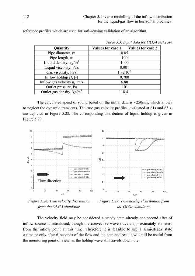
Chapter 5. Inverse modelling of the inflow distribution for the liquid/gas flow in horizontal pipelines 112
reference profiles which are used for soft-sensing validation of an algorithm.
Table 5.3. Input data for OLGA test case
Quantity Values for case 1 Values for case 2 Pipe diameter, m 0.05 Pipe length, m 100
Liquid density, kg/m3 1000 Liquid viscosity, Pa.s 0.001
Gas viscosity, Pa.s 1.82.10-5 Inflow holdup H, [-] 0.700
Inflow gas velocity ug, m/s 6.80 Outlet pressure, Pa 107
Outlet gas density, kg/m3 118.41 The calculated speed of sound based on the initial data is ~250m/s, which allows to neglect the dynamic transients. The true gas velocity profiles, evaluated at 61s and 63 s, are depicted in Figure 5.28. The corresponding distribution of liquid holdup is given in Figure 5.29.
0
1
2
3
4
5
6
7
8
9
10
0 20 40 60 80 100
L, m
Ug
, m/s
gas velocity, t=59s
gas velocity, t=60.1s
gas velocity, t=61s
gas velocity, t=63s
0
0.1
0.2
0.3
0.4
0.5
0.6
0.7
0.8
0 20 40 60 80 100
L, m
H, [
-]
gas velocity, t=59s
gas velocity, t=60.1s
gas velocity, t=61s
gas velocity, t=63s
Figure 5.28. True velocity distribution
from the OLGA simulator. Figure 5.29. True holdup distribution from
the OLGA simulator. The velocity field may be considered a steady state already one second after of inflow source is introduced, though the convective wave travels approximately 9 meters from the inflow point at this time. Therefore it is feasible to use a semi-steady state estimator only after 61seconds of the flow and the obtained results will still be useful from the monitoring point of view, as the holdup wave still travels downhole.
Flow direction

Chapter 5. Inverse modelling of the inflow distribution for the liquid/gas flow in horizontal pipelines
113
The obtained estimation results for two time instants are depicted in Figure 5.30 with the holdup distribution plotted at 62 and 63 seconds. It has been found that the main criterion for the successful estimation is defined by the proper description of the frictional pressure gradient. In that particular case, the Techo correlation (2.18) was able to provide the most reasonable results. The predictions of this correlation were first evaluated using open-loop runs with known inflow distribution, in order to match OLGA data. One can note a satisfactory estimation of the holdup field, despite certain model error introduced by OLGA. In the first part of the pipe, the estimated values overpredict OLGA data. Such behaviour might be caused either by constant gas density assumption used in the real-time estimator, or by a wrong choice of friction correlation tuning parameters.
0
0.2
0.4
0.6
0.8
1
0 20 40 60 80 100
L, m
H, [
-]
OLGA, 62s
Estimated, 62s
OLGA, 63s
Estimated, 63s
Figure 5.30. Estimated liquid holdup for OLGA data.
One can note a discontinuity in the estimated holdup profiles in the vicinity of the inflow source. Although we are not completely sure, this may be related to the fact that different grids are used in OLGA and in the real-time estimator, which leads to an inconsistency in the variables determination at the interface. Despite the positive preliminary results using artificial OLGA measurements, which clearly indicate the potential of using the proposed technique against “real-life” data, its applicability is still limited to an accurate prediction of multiphase friction factor. In particular, for a flow regime different from a considered homogeneous one, the frictional losses may be calculated incorrectly even if the complex slip models are used.
5.5. Conclusions
An analysis of the possibilities of using transient pressure data processing has been performed. The inflow of certain liquids from the reservoir to the wellbore produces a
Flow direction

Chapter 5. Inverse modelling of the inflow distribution for the liquid/gas flow in horizontal pipelines 114
transient response characterized by dynamic and kinematic waves. In particular, a pressure wave is generated which propagates in the direction both upstream and downstream the flow with the local speed of sound of the mixture. This speed of sound can be estimated from the transient pressure measurement. However, the information regarding inflow composition is missing. The propagation of the holdup wave, which defines the acoustic properties of the medium and hence the speed of sound, is much slower than the dynamic one. Therefore for a given inflow source, due to a delay in holdup wave propagation, it is impossible to extract the holdup information from the advancing pressure signal generated by the same inflow point. The estimation of the inflow composition may be performed by affecting the flow upstream the inflow point and providing dynamic waves, which move through the simulation domain over a given inflow point. The use of fully transient pressure information for flow rate estimation requires the processing of rapidly propagating wave signals that act on a very short time scale with a sufficient time resolution of the measurement. On the short term length scale the transient pressure information may be used to estimate the local inflow velocity. Alternatively, the inflow composition may be estimated using a simplified engineering approach from the pressure drop variation in the zone with the affected holdup. The performance of this technique is highly dependent on the value of the two-phase acoustic velocity, which should be high enough to provide very fast transients of pressure and velocity. The proposed semi-transient approach to a liquid holdup estimation has been tested on a series of simulation based test cases, which show the accuracy and reliability of the proposed algorithm. It has also been found that the efficiency of the Kalman filter depends on the prescribed model error matrix which is used as a tuning parameter. Even when the observations are heavily biased with model/measurement error, the estimator can efficiently correct the wrong model states. Unfortunately, in real applications the true error description is never completely available, and, hence, it is quite important to choose a proper error statistics which provide robustness of the filter. The results above are promising, though there is still some considerable work to be done before the real-time estimator can be implemented in practice. In particular, both small-scale laboratory experiments and field testing should be performed. It should be noted that for real applications, the influence of water phase should be taken into account and therefore water cut measurements are required.

Chapter 6. Estimation of the multiphase inflow for gas breakthrough control _________________________________________________________________________
115
6. Estimation of the Multiphase Inflow for Gas Breakthrough Control
6.1. Introduction
With the research methodologies and technologies emerging in oil and gas industry, production from complex reservoirs can be obtained. The increasing availability of sensors and actuators brings new possibilities for short-term production optimization. In particular, the implementation of the dynamic control strategies can maximize the output from the reservoir on the short term time scale by mitigating negative effects of various production instabilities in order increase the ultimate recovery. Such modern control systems combine data from different sources and require realistic physical modelling of the system performance. The production from long horizontal wells drilled in thin oil rims can be affected by gas coning, the phenomenon where the gas-oil contact of a reservoir moves towards a producing well (see Figure 6.1). At a certain moment the gas-oil contact will reach the well and gas breakthrough can happen causing a large gas inflow. Consequently, due to a rapid increase in gas rate, the gas phase starts to dominate production. In order to handle or prevent this, several strategies are available. Traditionally, the gas coning is avoided by limiting the pressure difference between wellbore and a reservoir to a certain value, which prevents the gas-oil contact to reach the well. This pressure drop corresponds to a certain production rate, which should not be exceeded in order to keep the production stable. The relevant quantities can be computed analytically [Guo et al., 1992; Ansari et al., 2006] or numerically [Benamara and Tiab, 2001]. Leemhuis et al., (2008) has implemented a feedback controller, which keeps the gas fraction below a certain value by continuously updating the settings of the wellhead choke. The analysis of different feedback control strategies using a coupled wellbore-reservoir dynamic simulator, performed by Nennie et al., (2009), has shown certain advantages of the fully controlled production over the intermittent one. Wells equipped with permanently installed sensors and actuators (surface chokes or inflow control valves) can be controlled via active control techniques. Jansen et al., (2002) suggested to influence the drawdown profile along the well through controlling the inflow. Another method, which was also considered in a paper by Leemhuis et al., (2008) considers direct downhole control by means of the inflow control valves. In this approach the inflow from reservoir to wellbore can be continuously adjusted in real-time. In case breakthrough occurs the gas producing zones of the wellbore can be simply isolated by means of inflow control valves (ICV). Due to the gravity the oil-gas contact will move away from the closed wellbore segment, which allows to continue the production. The

Chapter 6. Estimation of the multiphase inflow for gas breakthrough control _________________________________________________________________________ 116
important assumption used in this approach is that the flow rates can be measured downhole, though it is not always possible in real field applications. The down-hole gas fractions/velocities can be obtained from installation of down-hole equipment which provides real-time oil and gas production rates with sufficient spatial and temporal resolution. In particular, several multiphase flowmeters installed downhole can supply relevant information for ICV operation as they are capable of allocating the zones of oil, gas and water inflow in long horizontal wells. If these meters are too expensive or inaccurate, alternative solutions are needed. One can use the soft-sensing principles, i.e. to estimate gas fractions or other flow parameters from “traditional” meters, combined with relevant process model. The purpose of a soft-sensor or real-time estimator is to provide the operator with information of the downhole flow rate distribution in order to decide where breakthrough is occurring. The relevant ICV can then be closed.
Figure. 6.1. Schematic view of a horizontal well with a gas cone
(from Leemhuis et al., 2008). On the one hand, it is attractive to use the same technique, which was developed in Chapter 5 in order to estimate the multiphase rates in real-time. However, for that particular case that method may be inappropriate due to the following issues: 1) The gas coning is considered as a relatively fast-transient phenomenon from the point of the reservoir dynamics with the gas breakthrough time of order of hours. However, most of the wellbore related transient phenomena are acting on a completely different time scale, where the dynamics is defined by the value of corresponding eigenvalues. In addition, the technological limitations of ICV do not allow them to be closed much faster, it can take up to several hours to perform corresponding choke adjustments. Therefore, distinct transient signals in the wellbore, which are required for the soft-sensing algorithm, are missing in this case. 2) The stability issues of a fully explicit time integration scheme, which is usually used with wellbore flow simulators, require the time step to be chosen based on dynamic wave
Gas cone
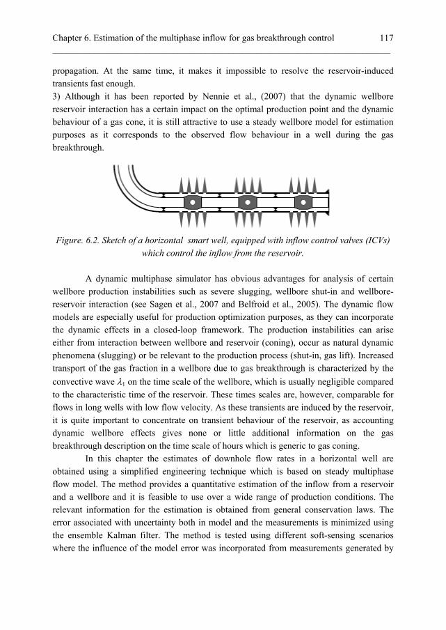
Chapter 6. Estimation of the multiphase inflow for gas breakthrough control _________________________________________________________________________
117
propagation. At the same time, it makes it impossible to resolve the reservoir-induced transients fast enough. 3) Although it has been reported by Nennie et al., (2007) that the dynamic wellbore reservoir interaction has a certain impact on the optimal production point and the dynamic behaviour of a gas cone, it is still attractive to use a steady wellbore model for estimation purposes as it corresponds to the observed flow behaviour in a well during the gas breakthrough.
Figure. 6.2. Sketch of a horizontal smart well, equipped with inflow control valves (ICVs)
which control the inflow from the reservoir.
A dynamic multiphase simulator has obvious advantages for analysis of certain wellbore production instabilities such as severe slugging, wellbore shut-in and wellbore-reservoir interaction (see Sagen et al., 2007 and Belfroid et al., 2005). The dynamic flow models are especially useful for production optimization purposes, as they can incorporate the dynamic effects in a closed-loop framework. The production instabilities can arise either from interaction between wellbore and reservoir (coning), occur as natural dynamic phenomena (slugging) or be relevant to the production process (shut-in, gas lift). Increased transport of the gas fraction in a wellbore due to gas breakthrough is characterized by the
convective wave 1 on the time scale of the wellbore, which is usually negligible compared
to the characteristic time of the reservoir. These times scales are, however, comparable for flows in long wells with low flow velocity. As these transients are induced by the reservoir, it is quite important to concentrate on transient behaviour of the reservoir, as accounting dynamic wellbore effects gives none or little additional information on the gas breakthrough description on the time scale of hours which is generic to gas coning. In this chapter the estimates of downhole flow rates in a horizontal well are obtained using a simplified engineering technique which is based on steady multiphase flow model. The method provides a quantitative estimation of the inflow from a reservoir and a wellbore and it is feasible to use over a wide range of production conditions. The relevant information for the estimation is obtained from general conservation laws. The error associated with uncertainty both in model and the measurements is minimized using the ensemble Kalman filter. The method is tested using different soft-sensing scenarios where the influence of the model error was incorporated from measurements generated by
Chapter 6. Estimation of the multiphase inflow for gas breakthrough control _________________________________________________________________________ 118
the OLGA simulator. At the end, the conclusions are given and recommendations for the future work are proposed.
6.2. Formulation of the estimation problem
The mathematical model to describe the flow, which is used to estimate the flow rates for gas coning control, originates from the transient drift-flux model described in Chapter 2. Just as in the previous chapter, some simplifying assumptions are made. Here, for simplicity, the influence of the wellbore transient phenomena is completely neglected and the dynamic effects are incorporated from the transient inflow. This leads to a set of simple differential equations providing simple mass and momentum balances. The transient
input from the reservoir, represented by the inflow sources Vl and Vg, defines values of
the states variables on the current time level. The flow model accounts for fluid acceleration and provides the necessary information regarding phase velocities using an algebraic slip law in the form of (2.28), where the flow regime impact is taken into account via variable drift-flux parameters. The gas density is calculated using the ideal gas law (2.20). The physical model can be formulated in the following state-space notation:
1 1,
k k kx f x u
(6.1)
Here u is the model input representing the inflow from reservoir to wellbore. x is the state vector evaluated on the previous time step. Using the primitive set of variables, the state vector can be written as
T
gx p u H (6.2)
Here p, ug and H are the vectors, representing pressure, velocity and liquid volume holdup related to the spatial grid. With the velocity of the gas phase known, the velocity of the liquid can be derived from the slip model (2.28). For that reason the liquid velocity ul is not included into the state vector. The estimation technique uses the information available from the measurements in order to calculate the approximated state vector components. For that particular problem the state vector consists of two parts. First, it includes the discrete values of the dynamic flow variables. In addition, the state vector includes unknown model input, which is defined by the inflow from the reservoir. The augmented form of the state vector is given by
T
i g i i Vg i Vl iX p u H (6.3)
Here i indicates the number of the cell defined by the numerical discretization. The measurements can be either defined at the surface (flow rate) or downhole (pressure). The measurements vector is therefore given by
Tdown surf
j jy y y (6.4)

Chapter 6. Estimation of the multiphase inflow for gas breakthrough control _________________________________________________________________________
119
Here j is the number of variables to be measured. The computational setup for the inverse problem is shown in Figure 6.3. It should be noted, that only the horizontal part of the well is being modelled, and the outflow measurements are assumed to be available directly at the outflow cross-section of the horizontal part.
Figure 6.3. Scheme of the computational setup for soft-sensing. Finally, the data assimilation problem can be formulated as follows: with the measurements (6.4) and the flow model the components of the augmented state vector (6.3) must be estimated.
The EnKF [Evensen, 1994] was used as soft-sensor. As mentioned above, this was done because of its (relative) ease of implementation while also being computationally fast enough. The ensemble size that was used was equal to Nens = 100.
Notes on the uniqueness of the estimation problem The use of the slow transients, generic to the gas coning process, and the subsequent assumption of slow wellbore dynamics has significantly simplified the forward modelling process. On the other hand, the transient signal carries information which is essential for the flow estimation. As the calculation of the multiphase flow rate requires the knowledge of three flow parameters, namely, fluid velocity, fluid density and volume fraction, three independent measurements are needed in order to obtain a unique result. Excluding the transient terms from the governing equations leaves out information on the wave propagation in the system, and makes the estimation problem ill-posed. In other words, due to the absence of transient data, which is implicitly incorporated in the governing equations, the estimator may easily fail to produce satisfactory results. In particular, for the case with a large number of grid blocks, multiple combinations of inflow/outflow of gas and liquid will result in a very large number of possible flow variables approximations, which satisfy the available measurements. One can try, in
Inflow from reservoir (liquid or gas)
liquid/gas mixture
,l gt t
surface measurements
downhole measurements

Chapter 6. Estimation of the multiphase inflow for gas breakthrough control _________________________________________________________________________ 120
principle, to reduce the uncertainty by incorporating additional measurement information, but very little can be measured additionally in order to keep the estimation technique cheap. In particular, the multiphase measurements taken on the surface may improve the data assimilation results by establishing a reference point for total inflow/outflow. Further improvement may be achieved by measuring certain flow parameters downhole (i.e. gas fractions, total flow rate) though it inevitably will increase the hardware costs of the estimator developed. If only pressure measurements are used, then special attention should be given to a pressure gradient between measurement points. For the case when one fluid is entering the grid block and other is leaving, the steady pressure signal is not sufficient for a data assimilation procedure. The number of possible solutions can be reduced if one imposes certain constraints together to be used with flow estimation algorithms. Although this theoretically will always provide a non-zero gradient between two measurement locations, additional data are still needed to make the formulation complete. More important, in many sequential data assimilation algorithms, such as Kalman filtering, the physical constraints can not be taken into account. The following engineering approach is proposed for the flow rate estimation of gas coning. In order to keep a non-zero gradient between sensors used for measuring the pressure, the inflow from the reservoir is prescribed by splitting the sources, which can be either liquid or gas. In addition, the amount of gas entering the wellbore per time step, expressed in terms of mass flow rate, is considerably less than the inflow corresponding to
the liquid phase. This holds for a reasonable range of fluid properties, where g<l.
Assuming that multiple pressure measurements are available in order to provide gradient information, the total amount of fluid (liquid and gas), which is entering the wellbore through the radial inflow can be estimated using the proposed data assimilation technique. On the other hand, the flowrate measurements at the outflow cross-section of the well provide an increment in liquid and gas flows on each time step considered. As the mass balance should be fulfilled, one can identify the inflow sources, and hence the distributions of liquid fraction and phase velocities along the length of the wellbore. At first sight, the analysis of the proposed scenario does not need to use any data assimilation algorithm limited as the amount of parameters to be estimated corresponds to the number of measurements available. However, the quality of the estimates should be improved as the measurement data are usually quite noisy and uncertain. Furthermore, the mathematical model to be used with the estimator needs a proper treatment of the model error in order to perform the estimation properly. The model error is associated with inflow sources to be estimated and errors related to the mismatch between the simple flow model used and real wellbore flow. In both cases a two-step procedure is needed, where first the preliminary values of inflow sources are obtained from the measurements, which are later corrected with the flow model used. This implies the implementation of the sequential data assimilation algorithm, where the dynamic data from noisy measurements are matched with

Chapter 6. Estimation of the multiphase inflow for gas breakthrough control _________________________________________________________________________
121
the predictions from the flow model. In principle the model used can be replaced or upgraded according to the user’s requests, which makes it possible to integrate the proposed approach into a closed-loop reservoir management framework. In this chapter the estimations of the multiphase flow rates has been obtained using an ensemble Kalman filter. The performance of the data assimilation algorithm is adjusted by adding a certain model noise to components of the state vector, which produce the largest uncertainty in a
simulation. These are in this case the inflow sources l and g.
It follows, that pressure measurements, both surface and downhole are required in order to estimate the inflow properly. In addition, it follows that the flow rate measurements at the outlet of the wellbore are also needed, as they provide necessary mass balances. On the one hand it may be disappointing as the corresponding equipment for such measurements is quite costly. On the other hand, it is still more reliable at the surface conditions rather than downhole.
6.3. Results and discussions
Test Case 1. Estimating flow rates under measurement error The first test case considered assesses the capabilities of the estimator to obtain the multiphase rates if the available measurements are corrupted with certain measurement error. Due to a lack of real experimental data, a set of synthetic measurements has been used for data assimilation. Here, a twin experiment concept has been implemented, where the same mathematical model was used both for generating the measurements with a predefined inflow distribution and the inverse modelling, when missing dynamic variables are estimated by means of the proposed algorithm. The major advantage of the proposed approach is that the obtained estimates can be compared to the real values of the model variables. Moreover, the simulations are performed with noise parameters which are fully quantitatively defined. Two scenarios are considered which deal with two-phase liquid/gas flow and the details of the initial data are given in Table 6.2. The sketch of the estimation setup is given in Figure 6.4 and Figure 6.5. The inflow profiles are given only as a reference since they are unknown and have to be estimated via the proposed data assimilation procedure. The essential difference between test cases is in the range of flow parameters used allowing to perform the simulations for different flow regimes. Both scenarios deal with estimation of flow rates along the length of the wellbore, where the distribution of multiphase parameters is affected by three inflow sources. The first case corresponds to a bubbly flow regime. This regime can be described by homogeneous no-slip model. The inflow for these cases, is represented by gas, which is injected in three locations of the wellbore linearly up to 0.48 kg/s from 20 to 50 minutes of production and afterwards kept constant for the last 10

Chapter 6. Estimation of the multiphase inflow for gas breakthrough control _________________________________________________________________________ 122
minutes. In the second scenario, where the flow is described by the drift-flux model with a slip, the gas sources near the inlet and outlet of the pipeline are replaced by liquid inflow. The maximum amount of liquid entering the wellbore is 2 kg/s for each inflow point, while for gas it is 0.02 kg/s.
l gF F 3000
0.16
1 2 3g g g
1200
2.00
l
l gF F
3000
0.02
1200
g
30001200
Figure 6.4. Computational setup for flow
rate estimation. Homogeneous flow. Figure 6.5. Computational setup for flow
rate estimation. Slug flow. The flow rate estimator has been tested using the following measurement layout. It is assumed that several downhole pressure measurements are available. Moreover, outflow information about flow rates is also known, giving the following measurement vector. The purpose of the flow rate measurements is to provide the mass balance, necessary to obtain unique inflow distribution. The data vector is given by
T
i g out outy p u H (6.5)
The number of pressure measurements was taken equal to the number of grid nodes obtained from the discretization. The velocity and liquid volume fraction measurements are located at the last grid block of the simulation domain. For both scenarios the wellbore was discretized with 12 grid blocks of constant length including 2 nodes for definition of the boundary conditions. The sampling interval for both considered cases was 60s.
Table 6.1. Measurement noise used in simulations
Uncertainty in pressure measurements 0.5%
Uncertainty in flow rate measurements 1.0%
The Kalman filter initialization is here based on the outflow values of velocity and liquid volume fraction, which are assumed to be know due to metering. Since all the pressure measurements are available, the pressure is initialized from the current pressure distribution. The synthetic measurements representing the downhole pressure and the liquid outflow flow rate are generated using equations of the same flow model. For the first test

Chapter 6. Estimation of the multiphase inflow for gas breakthrough control _________________________________________________________________________
123
case the noise-free measurements have been used. For a second test case the simulations were performed with a zero mean white Gaussian noise added to mimic the uncertainty in measurements. Values of measurement error used in the simulations are given in Table 6.1
Table 6.2. Initial data for the numerical experiments
Quantity Values for case 1
Values for case 2
Pipe diameter, m 0.05 0.05 Pipe length, m 100 100
Liquid density, kg/m3 1000 1000 Liquid viscosity, Pa.s 0.001 0.001
Gas reference density, kg/m3 118.9 11.93 Gas viscosity, Pa.s 1.82.10-5 1.82.10-5
Inflow liquid rate Fl, kg/s 9.5 1.98 Inflow gas rate Fg, kg/s 0.5 0.02
x1, m 15 15 x2, m 45 45 x3, m 75 75
Absolute roughness, m 0 0 Distribution parameter, [-] 1.0 1.2 Bubble drift velocity, m/s 0 0
6.5
7
7.5
8
8.5
9
9.5
0 20 40 60 80 100
L, m
U, m
/s
True, t=1800s.
Estimated, t=1800s
True, t=2400s
Estimated, t=2400s
True, t=3000s
Estimated, t=3000s
0.5
0.55
0.6
0.65
0.7
0.75
0 20 40 60 80 100
L, m
H, [
-]
True, t=1800s
Estimated, t=1800s
True, t=2400s
Estimated, t=2400s
True, t=3000s
Estimated, t=3000s
Figure 6.6. Comparison of estimated and
true flow velocity. Homogeneous flow. Figure 6.7. Comparison of estimated and true liquid fraction. Homogeneous flow.
The results of the simulation for the first scenario are given in Figures 6.6-6.7. Figure 6.6 shows the comparison between the estimated and true velocity distributions along the pipe length. The flow velocity is used to allocate the zones where a fluid is
Flow direction
Flow direction

Chapter 6. Estimation of the multiphase inflow for gas breakthrough control _________________________________________________________________________ 124
entering or leaving the wellbore. In order to identify the type of fluid, the distribution of the estimated liquid volume fraction is required. This is depicted in Figure 6.7. The results are given for three time instants 30 minutes, 40 minutes and 50 minutes. Since the pressure is available continuously from the measurements it is not depicted as an estimate. Similar plots obtained for a second test case are depicted in Figures 6.8-6.9. Here the same observation as in the previous chapter can be made: even if the measurements are corrupted with low values of measurement noise, the quality of estimates is still significantly affected. The results show that the proposed soft-sensor, for the given simplified formulation, is capable of reproducing the flow rate and liquid volume fraction distributions along the considered well part, even under a certain measurement error. Therefore, it is capable to detect multiple fluid sources as it is depicted in the figures. Similar results have been obtained for the second test case, where the drift-flux model with slip was used. Here due to a certain measurement noise, the quality of estimated deteriorates, though it is still possible to obtain reasonable estimates. Due to the induced uncertainty in pressure measurements, the flow rate estimator detects additional “parasite” inflow sources, which do not exist. As it is impossible to identify whether the calculated source is real or artificial, provided it satisfies the total mass balance, it affects the overall performance of the flow estimator. This can be observed in Figure 6.8, where one can note an almost continuous inflow from 20 to 60 meters and slightly inaccurate holdup predictions. However, as more measurements are used, the estimates are improved. The error accumulates to the (unknown) inflow section of the pipeline and decreases with the propagation of the solution, i.e. with the increase in incorporated measurement data.
1.5
2
2.5
3
3.5
4
4.5
5
5.5
6
0 20 40 60 80 100
L, m
U, m
/s
True, t=1800s.Estimated, t=1800s.True,t=2400sEstimated, t=2400True, t=3000s.Estimated,t=3000s
0.4
0.45
0.5
0.55
0.6
0.65
0.7
0.75
0.8
0 20 40 60 80 100
L, m
H, [
-]
True, t=1800s
Estimated, t=1800s
True, t=2400s
Estimated, t=2400s
True, t=3000s
Estimated, t=3000s
Figure 6.8. Comparison of estimated and true gas velocity. Slug flow regime. Noisy
measurement data.
Figure 6.9. Comparison of estimated and true liquid holdup. Slug flow regime. Noisy
measurement data.
Flow direction
Flow direction

Chapter 6. Estimation of the multiphase inflow for gas breakthrough control _________________________________________________________________________
125
Additional simulations were performed for the second scenario with a decreased sampling interval. The simulations were performed with a sampling time of 20s. The obtained results, which are depicted in Figure 6.10 and 6.11, shows the expected improvement in the quality of the estimates quality as more measurements are used in the estimation procedure. The results show that the proposed algorithm is capable to detect multiple fluid sources as it is depicted in the figures. The estimated liquid velocity is obtained from equation (2.28) and therefore it is as accurate as the predicted gas velocity. In that simulation case no attention has been paid to the flow regime. In reality, the flow may be described by the drift-flux model only in a limited range of flow conditions. Since both measurement generation and estimation are based on the same mathematical formulation, input data do not have to be physically realistic: any input set of parameters would result in fairly accurate soft-sensor performance. It should also be noted here that the added measurement error is the main source of the mismatch between estimated and true values. Performing noise-free simulations, however, would result in perfect estimation of relevant flow parameters.
1.5
2
2.5
3
3.5
4
4.5
5
5.5
6
0 20 40 60 80 100
L, m
U, m
/s
True, t=1800s.Estimated, t=1800s.True,t=2400sEstimated, t=2400True, t=3000s.Estimated,t=3000s
0.4
0.45
0.5
0.55
0.6
0.65
0.7
0.75
0.8
0 20 40 60 80 100
L, m
H, [
-]
True, t=1800s
Estimated, t=1800s
True, t=2400s
Estimated, t=2400s
True, t=3000s
Estimated, t=3000s
Figure 6.10. Comparison of estimated and
true gas velocity. Slug flow regime with reduce sampling time.
Figure 6.11. Comparison of estimated and true liquid fraction. Slug flow regime with
reduced sampling time.
Test Case 2. Influence of the model error The second study provides an assessment of the influence of the model error on the estimation results. A similar soft-sensing setup was used as depicted in Figure 6.3 with the measurement vector defined by (6.5). An important difference, however, was that the “true” well was not the same as the model used in the soft-sensor. The true wellbore measurements were obtained from the commercially available simulator OLGA. This was
Flow direction
Flow direction
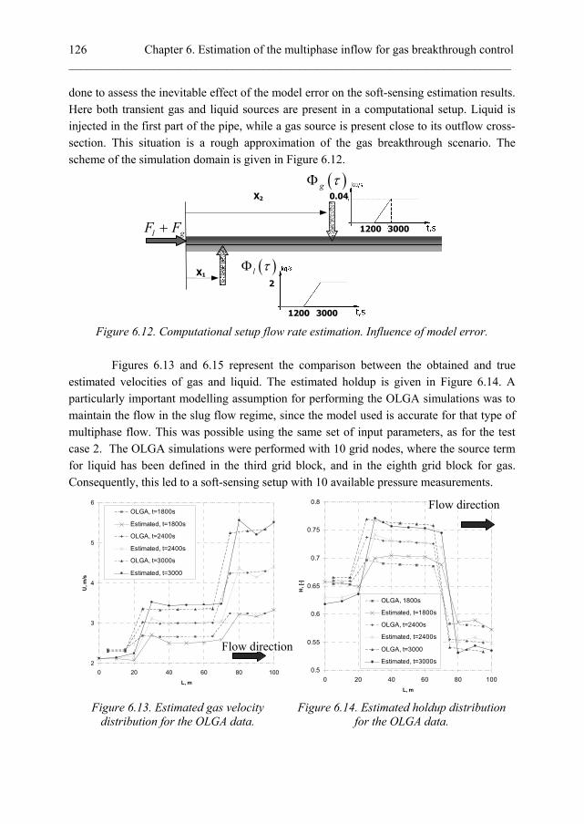
Chapter 6. Estimation of the multiphase inflow for gas breakthrough control _________________________________________________________________________ 126
done to assess the inevitable effect of the model error on the soft-sensing estimation results. Here both transient gas and liquid sources are present in a computational setup. Liquid is injected in the first part of the pipe, while a gas source is present close to its outflow cross-section. This situation is a rough approximation of the gas breakthrough scenario. The scheme of the simulation domain is given in Figure 6.12.
Figure 6.12. Computational setup flow rate estimation. Influence of model error.
Figures 6.13 and 6.15 represent the comparison between the obtained and true estimated velocities of gas and liquid. The estimated holdup is given in Figure 6.14. A particularly important modelling assumption for performing the OLGA simulations was to maintain the flow in the slug flow regime, since the model used is accurate for that type of multiphase flow. This was possible using the same set of input parameters, as for the test case 2. The OLGA simulations were performed with 10 grid nodes, where the source term for liquid has been defined in the third grid block, and in the eighth grid block for gas. Consequently, this led to a soft-sensing setup with 10 available pressure measurements.
2
3
4
5
6
0 20 40 60 80 100
L, m
U, m
/s
OLGA, t=1800s
Estimated, t=1800s
OLGA, t=2400s
Estimated, t=2400s
OLGA, t=3000s
Estimated, t=3000
0.5
0.55
0.6
0.65
0.7
0.75
0.8
0 20 40 60 80 100
L, m
H, [
-]
OLGA, 1800s
Estimated, t=1800s
OLGA, t=2400s
Estimated, t=2400s
OLGA, t=3000
Estimated, t=3000s
Figure 6.13. Estimated gas velocity
distribution for the OLGA data. Figure 6.14. Estimated holdup distribution
for the OLGA data.
l gF F
g 0.04
l
30001200
30001200
2
X2
X1
Flow direction
Flow direction

Chapter 6. Estimation of the multiphase inflow for gas breakthrough control _________________________________________________________________________
127
Obtained results are not as accurate as for the twin-experiment. However, it is still possible to allocate easily zones of liquid or gas inflow. A displacement of the estimated profiles with respect to the true ones is observed. This can be explained by the use of a different grid in the OLGA simulator and different interpolation of the flow variables between grid nodes and edges. The estimated velocity, both for liquid and gas phases, is quite accurate despite the fact that the OLGA solver is based on a rigorous two-fluid model, whereas the drift-flux formulation is employed for the estimation. The drift-flux parameters seem to be key values to provide accurate performance of a real-time estimator. For the cases, when they are not well defined, it is reasonable to include them into the state vector and estimate these parameters online from the data available [Bloemen et al., 2004], though it might increase the size of the state vector and decrease the robustness of the method. This leads to the conclusion that for estimation purposes complex flow modelling is not required. The flow model used as a soft-sensor may be simple enough to perform simulations in real-time, though it still should capture the main physics of the flow. It has been observed that since the information used for flow rate estimation is extracted from pressure measurements, it is quite important to account properly the friction factor correlation. In particular, preliminary runs in the open loop may be performed in order to validate the used model against OLGA data. The performance of the estimator is greatly affected by the added model noise, which represents uncertainty in unknown inflow sources. By means of a certain choice of the model error matrix it was possible to improve the qualities of the estimates. Since the true mismatch between model and OLGA is not known, it is very difficult to precisely define uncertainty in modelling, therefore the choice of model error which optimized the performance of real-time estimator is a topic of further research.
2
3
4
5
6
0 20 40 60 80 100
L, m
U, m
/s
OLGA, t=1800s
Estimated, t=1800s
OLGA, t=2400s
Estimated, t=2400s
OLGA, t=3000s
Estimated, t=3000
Figure 6.15. Estimated liquid velocity distribution for the OLGA data.

Chapter 6. Estimation of the multiphase inflow for gas breakthrough control _________________________________________________________________________ 128
Influence of flow regime uncertainty The preceding simulations showed that the proposed flow rate estimator can minimize the error associated both with measurement and model uncertainty and provided accurate estimates of flow variables. However, for the simulation tests considered, the major source of uncertainty was neglected. All the simulations were performed with a certain predefined flow regime, which was assumed to be known a priori. However, in the real-life applications the flow regime is not known by default which imposes the certain difficulty on estimation problems. In order to assess the influence of the flow regime on the quality of estimates the following test case is proposed. The measurements are generated via the twin experiment concept with the same layout as in Figure 6.6 where, however, the flow is described by different flow regimes. It is assumed that the flow in the first 40m of the wellbore length is bubbly, and slug in the rest. The flow regime dependency was incorporated using different sets of the distribution coefficient (C0=1.2 for slug flow and C0=1 for bubble flow). The flow rates are again estimated using the proposed flow model, though in this particular case, since the true flow regime is not known, the assumptions of slug flow is taken for all the wellbore elements during the estimation. The results of the simulations are given in Figures 6.16-6.17.
1.5
2
2.5
3
3.5
4
4.5
5
5.5
6
0 20 40 60 80 100
L, m
U, m
/s
True, t=1800s.Estimated, t=1800s.True,t=2400sEstimated, t=2400True, t=3000s.Estimated,t=3000s
0.4
0.45
0.5
0.55
0.6
0.65
0.7
0.75
0.8
0 20 40 60 80 100
L, m
H, [
-]
True, t=1800s
Estimated, t=1800s
True, t=2400s
Estimated, t=2400s
True, t=3000s
Estimated, t=3000s
Figure 6.16. Estimated gas velocity with
the flow regime uncertainty. Figure 6.17. Estimated gas velocity with the
flow regime uncertainty. The obtained results indicate that the uncertainty in flow regime introduces a major error in estimated variables. The predictions of liquid holdup and gas velocities are sufficiently accurate for the part of the well, which is properly modeled as a slug flow (see obtained estimates for the length interval 40-100 meters). The mismatch between estimated and true variables in this region is caused by the impact of model error, which was used as a
Flow direction

Chapter 6. Estimation of the multiphase inflow for gas breakthrough control _________________________________________________________________________
129
tuning parameter to account the uncertainty related to flow regime change. Since the exact boundary between flow regimes is not known, this model error is used for all the grid blocks. The estimates in the remaining zone only qualitatively describe the inflow. Liquid holdup is underpredicted, whereas the gas velocity is higher than the true one. As the liquid velocity is proportional to gas with drift-flux model, the estimates of this variable are not depicted on the figure. The quality of estimates can be improved by incorporating the flow regime dependency in the estimation algorithm. One can add the additional computational routine, which is used to predict the current flow regime. The state vector is then augmented by the values of the drift-flux parameters, which are estimated on-line together with dynamic state variables and inflow sources. For example, one can use the estimated superficial velocities in order to predict the existing flow regime by using certain flow regime transition criteria. Once the flow regime is obtained, the estimated superficial velocities can be corrected and the whole procedure repeated again iteratively. However, one can anticipate that stable operation of such algorithm requires additional independent measurements to be used in order to reduce the possibility of multiple solutions. One can analyze energy characteristics of the transient pressure fluctuations and establish the relationship between energy distribution of the signal and a flow pattern [Ding et al., 2006]. Application of the flow regime identification methods with flow rate estimators should be studied in detail during the future work.
Test Case 4. Predefined inflow It is common for all the test cases considered that initially no inflow sources are present in the simulation domain. Moreover, the assumption that both liquid and gas sources can not be present in a given location is too restrictive for real applications. The situation with complex inflow of both liquid and gas can be taken into account by separating the influence of these sources. In particular, if the inflow of one phase is already known and does not exhibit strong transient behaviour, it can be excluded from the estimation procedure. In order to evaluate the performance of the proposed algorithm the following case is proposed. The well initially produce a mixture of liquid and gas, with inflow of liquid continuously distributed along the length of the well. These sources are constant and they form the initial inflow profile which is assumed to be known. Afterwards, gas is rapidly entering the wellbore after 20 minutes of production in a location close to the outlet of the pipe. This inflow behaves in a similar way as it has been described in the previously considered cases. The simulations have been performed with the initial data relevant to bubbly flow regime and the synthetic measurements are obtained via a twin experiment.
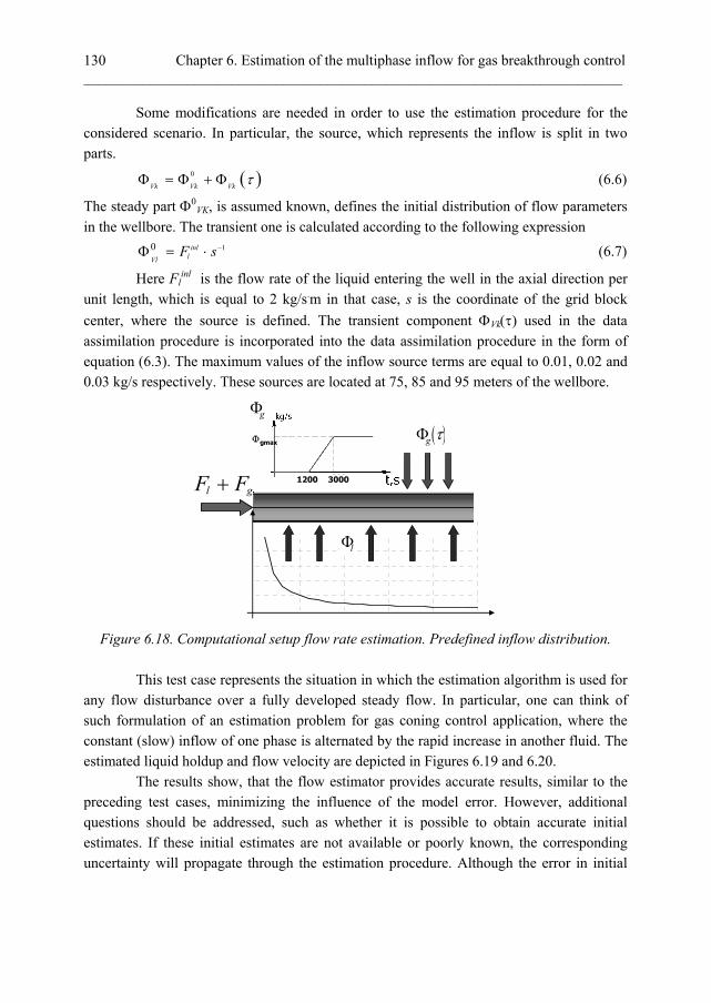
Chapter 6. Estimation of the multiphase inflow for gas breakthrough control _________________________________________________________________________ 130
Some modifications are needed in order to use the estimation procedure for the considered scenario. In particular, the source, which represents the inflow is split in two parts.
0
Vk Vk Vk (6.6)
The steady part VK, is assumed known, defines the initial distribution of flow parameters
in the wellbore. The transient one is calculated according to the following expression
10 inllVl
F s (6.7)
Here Flinl is the flow rate of the liquid entering the well in the axial direction per
unit length, which is equal to 2 kg/s.m in that case, s is the coordinate of the grid block
center, where the source is defined. The transient component Vk used in the data
assimilation procedure is incorporated into the data assimilation procedure in the form of equation (6.3). The maximum values of the inflow source terms are equal to 0.01, 0.02 and 0.03 kg/s respectively. These sources are located at 75, 85 and 95 meters of the wellbore.
l gF F 3000
gmax
g
1200
g
l
Figure 6.18. Computational setup flow rate estimation. Predefined inflow distribution.
This test case represents the situation in which the estimation algorithm is used for any flow disturbance over a fully developed steady flow. In particular, one can think of such formulation of an estimation problem for gas coning control application, where the constant (slow) inflow of one phase is alternated by the rapid increase in another fluid. The estimated liquid holdup and flow velocity are depicted in Figures 6.19 and 6.20. The results show, that the flow estimator provides accurate results, similar to the preceding test cases, minimizing the influence of the model error. However, additional questions should be addressed, such as whether it is possible to obtain accurate initial estimates. If these initial estimates are not available or poorly known, the corresponding uncertainty will propagate through the estimation procedure. Although the error in initial

Chapter 6. Estimation of the multiphase inflow for gas breakthrough control _________________________________________________________________________
131
estimates can be represented by a certain model error, it will not be minimized using a data assimilation algorithm.
1.5
2
2.5
3
3.5
4
4.5
5
5.5
6
0 20 40 60 80 100
L, m
U, m
/s
True, t=1800s.Estimated, t=1800s.True,t=2400sEstimated, t=2400True, t=3000s.Estimated,t=3000s
0.2
0.3
0.4
0.5
0.6
0.7
0.8
0 20 40 60 80 100
L, m
H, [
-]
True, t=1800s
Estimated, t=1800s
True, t=2400s
Estimated, t=2400s
True, t=3000s
Estimated, t=3000s
Figure 6.19. Estimated gas velocity with
predefined inflow distribution Figure 6.20. Estimated gas velocity with the
predefined inflow distribution
6.4. Conclusions
By means of two case studies, some limitations and possibilities of soft-sensor multiphase flow meters have been discussed. The proposed real-time estimator is based on the ensemble Kalman filter approach and requires as the input a simple model of the multiphase wellbore flow together with pressure measurements available downhole and one volume fraction and velocity measurement at the outflow. It has been shown, that for a two-phase flow formulation it is possible to reconstruct the distributions of the flow velocity and liquid volume fraction along a pipe and to allocate the inflow of certain fluids in specific location along it. The results indicate that the proposed method is stable for a certain range of wellbore operational conditions, and capable of taking into account measurement and model error. The applicability of the method is defined by the two following limitations. First, it requires the knowledge of the initial inflow distribution, which sometimes is difficult to obtain. Second, and more important, the uncertainty in flow regime seems to be a key-factor in obtaining fine estimates. If the flow regime is not known, the method easily fails.
Flow direction

Chapter 7. Conclusions and future work _____________________________________________________________ 132

Chapter 7. Conclusions and future work _________________________________________________________________________
133
7. Conclusions and Future Work The aim of this thesis is to develop a multi-phase soft-sensor, with a focus on horizontal flows of oil/gas mixtures and to assess its performance. The proposed sensor focuses on the analysis of transient responses induced by wellbore-reservoir interaction. Here the conclusions with regards to the research questions formulated in Chapter 1 are given. The chapter is also supplemented with suggestions for future work.
7.1. Modelling and Simulations
Dynamic wellbore modelling This thesis employs a simple one-dimensional approach to describe the transient phenomena in a multiphase wellbore flow. This is a common technique to deal with multiphase flows, for which due to lack of computational resources, or necessity of robust simulation response, the use of 3D formulations is impractical. The use of the one-dimensional flow approximation simplifies greatly the programming issues, however, the physical modelling becomes more uncertain. In this case the reduction of the multi-dimensional behaviour needs to be compensated by additional closure equations, which are often obtained from experiments and have a limited accuracy and range of applicability. Following from the multi-fluid model, which is the most straightforward and rigorous one-dimensional formulation, more models are derived which can be used for specific applications. The homogeneous no-slip model consists of a mass and momentum balance for the mixture. The no-pressure-wave model considers the transient continuity equations for the separate phases and a static force balance for the mixture. The drift-flux formulation consists of fully transient equations for mass balances of individual phases and the momentum equation written for the mixture. The homogeneous, drift-flux and two-fluid models are hyperbolic for a wide range of flow parameters with real and distinct eigenvalues corresponding to characteristics. For a drift-flux formulation two of these characteristics represent rapid pressure waves one propagating in upstream and one in downstream direction of the flow. One characteristic, which is not available in a homogeneous model, corresponds to the holdup wave and its transport is defined by an average velocity of the gas phase. The no-pressure wave model is of mixed hyperbolic-parabolic type, in which the only eigenvalue corresponds to the propagation of the composition wave. These eigenvalues represent the directions in which information is propagated in the physical domain with a certain speed. The speed of the dynamic waves is defined by the acoustic properties of the propagation medium and it is expected to give information about the flow structure via the analysis of the transient behaviour of pressure and velocity.
Chapter 7. Conclusions and future work _____________________________________________________________ 134
Flux splitting The models considered can be solved numerically using splitting of the flux components according to the obtained eigenvalues, thereby explicitly accounting for the directions in which the information is transported. The shock capturing properties of the flux splitting schemes are improved by using high resolution schemes with flux limiters. The problem of a direct use of a flux splitting method is associated with the structure of the governing equations, since the proposed method was initially developed for homogeneous systems. With the drift flux model the source terms are present in both in the continuity and momentum equations, which leads to incorrect steady-state solution. In particular, the inflow from the reservoir, represented by a source in the continuity equation, produces local oscillations on the density profile. It is suggested to handle this problem by introducing the integrated source, which retains an exact balance with the flux gradients and keeps the conservative properties of the numerical solution. The developed algorithm has been applied to a series of test cases. The proposed solver has been verified employing some reference solutions and data provided by the commercially available OLGA simulator. One of the advantages of the proposed technique is that the algorithm is applicable to any system of heterogeneous hyperbolic equations.
7.2. Data Assimilation
All the flow models considered are represented by sets of partial differential equations, which should be converted into a state-space form by using relevant computational techniques. Among the variety of time integration schemes used, one can distinguish between the implicit Euler scheme, which is unconditionally stable for the whole range of time steps, and the explicit Euler scheme, which strongly defines the maximum value of the allowed time step. More important, the usage of these schemes leads to a completely different formulations of the state-space form, which might be inappropriate from the point of its usage with sequential data assimilation. The performance of the real-time parameter estimation based on the extended Kalman filter has been assessed. Using a model of the single phase oil flow in a porous medium formulated as a first-principles model, three types of estimators were derived: implicit, explicit and semi-implicit. All these were designed for parameter estimation purposes, i.e. to estimate the radial distribution of permeability in a reservoir with a single producing well, based on transient pressure measurements downhole. The fully implicit estimator uses an implicit Euler scheme to obtain both the state-space form of the model equations and the model Jacobian used for the computation of the error covariance matrices. This scheme is unconditionally stable and no limitations are imposed on the integration time step size. Via simulation based test cases it has been shown

Chapter 7. Conclusions and future work _________________________________________________________________________
135
that the choice of initial conditions (the initial permeability distribution) is crucial for a satisfactory performance of the fully implicit estimator. For the cases where good initial conditions are not available, the filter diverges. This problem can be overcome by imposing smaller values for the time step. This, however, diminishes the main advantage of the fully implicit approach – the capability to run the simulations without time step limitations. In contrast, the fully explicit estimator, which uses an explicit Euler scheme to obtain both the state-space form of the model equations and the model Jacobian, does not exhibit this dependency of the estimation accuracy on the initial conditions. However, it is bounded to an upper limit on the integration time step size because of numerical stability considerations. To eliminate the disadvantages of the two methods above and to reinforce their strong parts, a semi-implicit method has been proposed. In this approach the implicit Euler scheme is used for the computation of the model update step of this estimator while the explicit Euler scheme is used for computing the Jacobian needed for the computation of the error covariance matrix update in this step. Via simulation based test cases it has been demonstrated that this new estimator is only weakly affected by initial conditions and can be used for an extended range of time steps.
7.3. Soft-Sensing
The inflow of certain fluids from the reservoir initiates dynamic and kinematic waves which propagate in the wellbore. As the pressure wave travels both upstream and downstream the inflow location with a two-phase speed of sound defined by the acoustic properties of the mixture, the corresponding transient pressure measurements performed along the length of the pipeline may provide the information on the two-phase sonic speed. However, this gives very little insight in terms of estimation of inflow composition, i.e. the type of fluid which is entering the wellbore. The distribution of holdup, which defines the acoustic properties of the two-phase medium, is significantly delayed compared to the pressure waves, as its propagation speed is defined by the gas velocity, which is much lower than the mixture speed of sound. Due to this mismatch, it seems impossible to use the information from the same inflow source in order to estimate liquid holdup and flow velocity. The information on the flow velocity may be obtained from measuring the local pressure increase due to flow acceleration, which is however rapidly smeared out due to frictional effects in the wellbore. The liquid fraction due to inflow may be estimated from a simplified engineering approach, where the variation of the pressure drop due to propagation of holdup wave is considered. This can be performed when the acoustic velocity is high enough to provide very fast transient behavior of pressure and velocity. Secondly, this method will only work

Chapter 7. Conclusions and future work _____________________________________________________________ 136
if the inflow is rapid, so it provides distinct signal which can be measured by the sensors. As the dynamic effects of the wellbore flow are not fully taken into account, it is reasonable to switch from a complex drift-flux formulation to a simpler no-pressure wave model. The performance of the proposed technique has been evaluated via a series of test cases, which all aim to estimate the distribution of the liquid fraction in a segment of a horizontal well under various inflow conditions. As the estimator the extended Kalman filter has been used. The proposed method has also been tested against data generated by the wellbore simulator OLGA. The model error matrix is chosen by the user and used for the tuning of the Kalman filter. It is important to note, that due to discrepancy in speeds of dynamic and kinematic waves, they cannot be estimated at the same time even if exhaustive computational tools are available. The velocity wave is decoupled from the holdup one, and therefore it appears that a simple homogeneous model is sufficient to estimate the flow velocity based on the transient pressure measurements. For the cases when the holdup wave is important, use of a simple no-pressure-wave model, which focuses on the convective transport, can be made. If the inflow from reservoir needs to be considered on a different time scale, which does not produce any transient response in the wellbore, another technique is needed. This is especially important for gas coning control applications, when the process is governed by the slow reservoir dynamics. In that case the required information is obtained from multiple pressure measurements downhole supplemented with a single multiphase flow measurement at the surface. The performance of the technique has again been tested using simulation based test cases, and satisfactory performance has been demonstrated. The numerical experiments showed that the technique was able to correct the model error, induced by the OLGA simulation, if the friction factor correlation was specified correctly. The important limitation of both considered methods is related to uncertainty in the flow regime. This should be known in advance, or be somehow integrated in the estimation procedure in order to provide fine performance. Secondly, both methods use the initial distributions to some extent on the inflow distribution (i.e. flow rates and liquid fractions along the well). This information, which may easily be missed in real-life applications, was found to be crucial. The results obtained indicate that the soft-sensing techniques will not completely replace existing measurement equipment nor will be used as separate source of information, as in this case too many simplifying assumptions have to be made. It is rather more feasible to combine the output of the existing multiphase flow meters, installed downhole or at the surface, and relevant flow models in order to improve overall performance of the hardware instrumentation. The multiphase meters can then operate with increased accuracy, be able to work over a wider range of flow conditions, or cover flow regimes where direct measurements are unfeasible.

Chapter 7. Conclusions and future work _________________________________________________________________________
137
7.4. Suggestions for Future Work
1) The semi-implicit Kalman Filter introduced in Chapter 4 has been initially developed for single phase flow in porous media, which is a typical example of parabolic differential equation, in which diffusion is dominating. In the area of multiphase wellbore flow, the convection is more important, therefore one should think of developing a similar semi-implicit technique for multiphase flow estimators. The main obstacle to such an approach is that the fully implicit schemes are generally more diffusive and hence may not be used for problems with moving shocks and other discontinuities. On the other hand, the effect of numerical diffusion can be mitigated by high resolution numerical schemes and there is still big potential for performing simulations without time step limitation. 2) Although it was at first expected that a drift-flux model was needed in order to obtain relevant estimates, the presented results have been obtained with simpler physical models. It is recommended to use the drift-flux approach (or more complex two-fluid model) when the combined estimation of velocity and holdup is required. This is especially important for highly heterogeneous flows for which the estimates of the velocity of the phases are coupled to the liquid fraction. It is also important to consider more complex models, which are applicable for all range of flow rates, and in which wellbore inclination and the flow regime dependency can be easily accounted for by incorporating rigorous transition mechanisms. Moreover, in real industrial systems, the wellbore profile is usually more complex than the idealized systems considered in this thesis. Multiple flow obstructions and rapid changes of the wellbore geometry affect greatly the dynamic inflow response. The performance of a semi-steady state technique is also affected, as local wellbore resistances might affect the holdup predictions. Last remark regarding wellbore modelling is related to the flow regime. It is expected to have a slug flow dominating in oil/gas wells, though the proposed drift-flux model gives only an averaged description of the phase distribution, with separate slugs not taken into account. The flow regime itself is another source of uncertainty as it should be known in advance in order to provide accurate estimates. Therefore it is suggested to incorporate the flow regime in estimation procedure or to obtain flow regime information using other methods. 3) Finally, one should think of validation of the proposed approach. For that reasons a experimental setup has been built in the Multi-Scale Physics department of the Delft University of Technology, which is outlined in the Appendix B. Unfortunately, the experimental part of this project turned out to be rather rudimentary, and therefore results have not been included in this thesis as the outcome of the experimental work. The purpose of the experimental setup may be given as follows:
To analyze the existing flow patterns, define the flow regime map and calculate attenuation coefficients (i.e. friction factor) and phase velocities;

Chapter 7. Conclusions and future work _____________________________________________________________ 138
To obtain data required for multiphase model inversion, i.e. generate and measure kinematic and dynamic waves.
The measurements of the pressure wave can be used to estimate the flow velocity while the static pressure drop provides the estimation of the holdup front. The latter can then be verified using a series of liquid fractions measurements, which should be available at several locations along the wellbore. The major advantage of a controlled experiment is that the model error associated with various flow phenomena can be identified and accounted for separately in the estimation.

Bibliography _________________________________________________________________________
139
Bibliography Aamo, O.M., Eikrem, G.O., Siahaan, H.B., Foss, B.A. (2004). Observer design for multiphase flow in
vertical pipes with gas lift – theory and experiments. Journal of Process Control, 15, pp 247-257. Aggrey, G. and Davies, D.R. (2008). Real-time water detection and flow rate tracking in vertical and
deviated intelligent wells with pressure sensors. SPE paper 113889. EAGE Annual conference and Exhibition, Rome
Alimonti, C. and Bilardo, U. (2001). Measurement of three-phase flow rates using neural network approach, Proc. 4th international conference on Multiphase flow, New-Orleans, USA.
Antoulas, A.C., Sorensen, D.C., Gugercin, S. (2001). A survey of model reduction methods for large-scale systems. Contemp. Math. 280, 193–219.
Ansari, A.M. (1994). A comprehensive mechanistic model for two-phase flow in wellbores, SPEPF, Trans.AIME, 297.
Ansari, R.Z., Johns R.T. (2006). Steady-state coning solutions with multiphase wells and reservoir boundaries. SPE paper 99896, SPE/DOE symposium on improved oil Recovery, Tulsa. USA
Aspelund, A., Midttveit, O., and Richards, A. (1996). Challenges in Downhole Multiphase Measurements. SPE paper 35559, Proc. European production operations conference and exibition, Stavanger.
Atkinson, D.I., Berard, M., Segeral, G. (2000). Qualification of a nonintrusive multiphase flow meter in viscous flows. SPE paper 63118, Proc. Annual technical conference and exhibition, Dallas, USA.
Aziz K., Settari, A. (1979). Petroleum Reservoir Simulation, London, UK: Applied Science Publ. Baudin, M., Berthon, C., Coquel, F., Masson, R. Tran, Q.H. (2005a). A relaxation method for two-
phase flow models with hydrodynamic closure law, Numer. Math., 99, 411-440. Baudin, M., Coquel F. and Tran, Q.H. (2005b). A semi-implicit relaxation scheme for
modeling two-phase flow in a pipeline. SIAM J. Sci. Comput. 27(3), 914-936. Barnea, D. (1987). A unified model for predicting flow-pattern transitions for the whole range of pipe
inclinations. International Journal of Multiphase Flow, 13(1), 1-12. Belfroid, S.P.C., Sturm, W.L., Alberts, G.J.N. Peters M.C.A.M., and Schiferli, W. (2005) Prediction
of Well Performance Instability in Thin Layered Reservoirs. SPE paper 95835 SPE Annual Technical Conference and Exhibition, Dallas, Texas
Benamara, A., Tiab, D. (2001). Gas coning in vertical and horizontal wells, a numerical approach. SPE paper 71026, SPE Rocky Mountain Petroleum Technology Conference, Colorado, USA
Bendiksen, K., Malnes, D., Moe, R. and Nuland, S. (1991). The dynamic two-fluid model OLGA: theory and application. SPE production Engineering, 6, 171-180.
Bendiksen, K.H. (1984). An experimental investigation of the motion of long bubbles in inclined tubes. International Journal of Multiphase Flow, 10(4) pages 467-483.
Bendiksen, K.H., Malnes, D., Nydal, O.J. (1996). On the modelling of slug flow. Chem. Eng. Comm. 141–142, 71–102.
Bermudez, A., Vazquez, M.E. (1994). Upwind methods for hyperbolic conservation laws with source terms. Computers Fluids, 23(8), 1049 –1071.
Bestion, D., Micaelli, J.C. (1986). A two-fluid stratified model suitable for a pressurized water reactor safety code. 4th Miami Int. Symp. on Multiphase Transport and Particulate Phenomena.
Bloemen, H.H.J., Belfroid, S.P.C., Sturm, W.L. and Verhelst, F.J.P.C.M.G. (2004). Soft sensing for gas-lift wells. In: Paper SPE 90370, Presented at the SPE Annual Technical Conference and Exhibition, Houston, Texas, USA.
Bibliography _________________________________________________________________________ 140
Bonizzi, M. (2003). Transient one-dimensional modelling of multiphase slug flows. PhD Thesis, Imperial College London, UK.
Boure, J.A. (1997). Wave phenomena and one-dimensional two-phase flow models. Multiphase Sci. Tech. 9, 1-107.
Brauner, N. (1998). Liquid-liquid two-phase flow. HEDU - Heat Exchanger Design Update. Ch. 2.3.5, pp. 1 – 40.
Brill, J.P. and Mukherjee, H. (1999). Multiphase flow in Wellbores. Monograph Series, SPE, Richardson, Texas.
Brouwer, D.R. and Jansen J.D. (2004). Dynamic optimisation of water flooding with smart wells using optimal control theory, SPE J.
Brown, G.A., Kennedy, B., Meling, T. (2000). Using fibre-optic distributed temperature measurements to provide real-time reservoir surveillance data on Wytch Farm field horizontal externded-reach wells. SPE paper 62952
Brunone, B., Golia, U. M., and Greco, M. (1991). Some remarks on the momentum equation for fast transients. Proc. Int. Conf. on Hydr. Transients With Water Column Separation, IAHR, Valencia, Spain, 201–209.
Chen, Y. (2001). Modelling gas-liquid flow in pipes: flow pattern transitions and drift-flux modelling. MSc Thesis, Stanford University, USA.
Chen, G.Q., Toro, E.F. (2004). Centred schemes for non-linear hyperbolic equations, Journal of Hyperbolic Differential Equations 1 (1), 531-566.
Chacón Rebolo, T., Fernández-Nieto, E.D., Gómez Mármol, M. (2003). A flux-splitting solver for shallow water equations with source term. Int. J. Numer. Meth. Fluids, 41, 1-33.
Clark, N.N., Egmond, J.W. van, Nebiolo, E.P. (1990). The drift–flux model applied to bubble columns and low velocity flows. International Journal of Multiphase Flow, 16, 261–279.
Coddington P., Macian R. (2002). A study of the performance of void fraction correlations used in the context of drift-flux two-phase flow models, Nuclear Engineering and Design, Volume 215 (3), 199-216.
Collins, R. (1978). The motion of a large gas bubble rising through liquid flowing in a tube. J. Fluid Mech., vol. 89, part 3, pp. 497-514.
Crassidis, J.L, Junkins, J.L. (2004). Optimal Estimation of Dynamic systems. Chapman & Hall/CRC. Dake, L.P. (1978). Fundamentals of Reservoir Engineering. Elsevier. Davies, R.M., Taylor, G.I. (1950). The mechanics of large bubbles rising through liquids in tubes.
Proc. R. Soc. Lond. A 200, 375–390. Ding, H. and Huang, Z. and Song, Z. and Yan, Y. (2007). Hilbert-Huang transform based signal
analysis for the characterization of gas-liquid two-phase flow. Flow Measurement and Instrumentation, 18 (1). 37-46.
Duns, H., Ros, N.C.J. (1963). Vertical flow of gas and liquid mixtures in wells. Proc. Sixth world petroleum congress, Tokyo 451.
De Henau, V., Raithby, G.D. (1995). A study of terrain-induced slugging in two-phase flow pipelines. International Journal of Multiphase Flow, 21(3), 365-379.
Erickson, D., Twaite, D. (1996) Pipeline Integrity Monitoring System for Leak Detection, Control, and Optimization of Wet Gas Pipelines. SPE paper 36607. Proc. SPE Annual Technical Conference and Exhibition, Denver, USA.
Ertekin, T., Abou-Kassen, J.H., King, G.R. (2001). Basic Applied Reservoir Simulation. Society of Petroleum Engineers, Richardson.
Evensen, G. (1992). Using the extended Kalman Filter with a multilayer quasi-geostrophic ocean model, J. Geophys. Res., 97, 17905-17925.

Bibliography _________________________________________________________________________
141
Evensen, G. (1994). Sequential data assimilation with a nonlinear quasi-geostrophic model using Monte Carlo methods to forecast error statistics, J. Geophys. Res., 99(C5), 10143–10162.
Evje, S., Fjelde, K.K. (2002). Hybrid flux-splitting schemes for a two-phase flow model, Journal of Computational Physics, Volume 175 (2) 20, pp. 674-701.
Evje, S., Flåtten, T. (2007). On the wave structure of two-phase flow models. SIAM J. Appl. Math. Volume 67 (2), pp. 487-511.
Faille, I., Heintze, E. (1999). A rough finite volume scheme for modeling two-phase flow in a pipeline, Computers & Fluids 28, pp. 213–241.
Falk, K., Gudmundsson, J.S. (1998). Pressure waves through gas-liquid flow in wells and pipelines. SPE paper 52060. Proc. SPE European petroleum conference, The Netherlands.
Falk, K. (1999). Pressure pulse propagation in gas-liquid pipe flow. Dr. Ing. thesis, Department of Petroleum Engineering, NTNU, Norway.
Falk, K., Gudmundsson, J.S. (1999). Multiphase pressure pulses for quick-acting valves: offshore testing. SPE paper 56526, Proc. SPE Annual Technical Conference and Exhibition, Houston, USA.
Ferziger, J.H., Peric, M. (2002). Computational Methods for Fluid Dynamics. Springer, 3rd edition. Fjelde, K.K., Karlsen, K.H. (2002). High-resolution hybrid primitive-conservative upwind schemes
for the drift flux model, Computers & Fluids, Volume 31 (3). Flatten, T., Munkejord, S.T. (2006). The approximate Riemann solver of Roe applied to
a drift-flux two-phase flow model. ESAIM, 40(4), 735-764. França, F., Lahey, R.T. (1992). The use of drift-flux techniques for the analysis of horizontal two-
phase flows. Int. J. Multiphase Flow 18, pp. 787–801. Gascon, Ll., Corberan, J.M. (2001). Construction of second-order TVD schemes for nonhomogeneous
hyperbolic conservation laws, Journal of Computational Physics, 172(1), 261-297. Gavage, S.B. (1991). Analyse numerique des modeles hydrodynamiques d’ecoulements diphasiques
instationnaires dansles reseaux de production petroliere. These, ENS Lyon France. Ghidaoui, M.S., Zhao, M., McInnis, D.A., Axworthy, D. H. (2005). A review of water hammer
theory and practice. Appl. Mech. Rev., 58, 49–76. Glandt, C.A. (2003). Reservoir aspects of smart wells. SPE paper 81107, Proc. SPE Latin American
and Caribbean Petroleum Engineering Conference, Trinidad, West Indies. Goh, K.C., Dale-Pine, B., Yong, I., van Overschie, P., Lauwerys, C. (2008). Production surveillance
and optimization for multizone smart wells with data driven models, SPE paper 112204, Proc. SPE Intelligent Energy Conference and Exhibition, Amsterdam.
van der Gees, R., Broman, W.H., Johnson, T.L. and Fleming, R.H., Alle,n J.O. (2001). Reliability through data reconciliation. Proc. Offshore Technology conference and exhibition, Houston, USA.
Green, D.W. and Willhite, G.P. (2003). Enhanced Oil Recovery. SPE Textbook Series Vol. 6, Richardson, TX, USA,
Gudmundsson, J.D. and Celius, H.K. (1999). Gas-liquid metering using pressure pulse technology. paper SPE 56584. Proc. SPE Annual Technical Conference and Exhibition, Houston, Texas.
Guo, B., Molinard, J.E., Lee, R.L. (1992). A General solution of gas/water coning problem for horizontal wells”, paper SPE 25050 pp 327-337
Hagedorn, A.R. Brown, K.E. (1965). Experimental study of pressure gradients occurring during continuous two-phase flow in small-diameter vertical conduits. JPT 475, AIME, 234.
Hamoud, A.A., Boudi, A., Al-Qahtani, S.D. (2008). New application of an inline separation technology in a real wet gas field. SPE paper 117459. Proc. International Petroleum Exhibition and conference, Abu Dhabi, UAE.
Bibliography _________________________________________________________________________ 142
Hanssen, B.V., Torkildsen, B.H. (1995). Status of the Framo subsea multiphase flowmeter. Proc. 13th North Sea Flow measurement workshop.
Harmathy, T.Z. (1960). Velocity of large drops and bubbles in media of infinite or restricted extent, A.I.Ch.E. Journal, 6 (2), 281-288.
Hatton, G.J. (1997). Multiphase flow meters and application trends. Proc. offshore technology conference and exhibition, Houston, USA.
Henry, R.E. (1970). Pressure wave propagation in two-phase mixtures. in Chemical Engineering progress symposium, vol. 102, pp. 1-10.
Hewitt, G.F., Harrison, P.S., Parry, S.J., and Shires, G.L. (1995). Development and testing of the “Mixmeter” multiphase flow meter. Proc. 13th North Sea Flow Measurement Workshop, Lillehammer, Norway.
Hirsch, C. (1990), Numerical Computation of Internal and External Flows, vol. 2, Wiley. Houtkamer, P.L., Mitchel, H.L. (1998). Data assimilation using an ensemble Kalman filter technique.
Monthly Weather review. Vol. 126, 796-911. Hubbard, M.E., García-Navarro, P. (2000). Flux difference splitting and the balancing
of source terms and flux gradient. J. Comput. Phys. 165, 89-125. Jansen, F.E., Shoham, O., Taitel, Y. (1996). The elimination of severe slugging - experiments and
modelling. International Journal of Multiphase Flow, Volume 22(6), November 1996, Pages 1055-1072,
Jansen, J.D., Bosgra, O.H. and Van den Hof, P.M.J. (2008). Model-based control of multiphase flow in subsurface oil reservoirs, Journal of Process Control, 18, 846-855.
Jansen, J.D., Wagenvoort, A.M., Droppert, V.S., Daling, R., and Glandt, C.A. (2002). Smart Well Solutions for Thin Oil Rims: Inflow Switching and the Smart Stinger Completion paper SPE 77942, presented at the SPE Asia Pacific Oil and Gas Exhibition, Melbourne, Australia.
Jazwinski, A.H. (1970). Stochastic Processes and Filtering Theory. Academic Press, New York. Julier, S., Uhlmann, J. and Durrant-Whyte, H.F. (2000). A new method for the non-linear
transformation of means and covariances in filters and estimators, IEEE Transcations on Automatic Control, 45(3), 477-482.
Ishii, M. (1977). One-dimensional drift-flux model and constitutive equations for relative motion between phases in various two-phase flow regimes. ANL-77-47, USA, 1977.
Ishii, M. and Hibiki, T. (2006). Thermo Fluid Dynamics of Two-phase Flow. Springer Science Business Media.
Kalman, R.E. (1960). A new approach to linear filter and prediction theory,” Trans. ASME, Series D, J. Basic Eng., V. 82, pp. 35 – 45.
Kettle, R.J., Ross, D., Deznan D. (2002). The Multiphase flowmeter, a tool for well performance diagnostics and production optimization. SPE paper 77893, Proc. SPE Asia and Pacific oil and gas conference.
Koren, B. (1993). A robust upwind discretisation method for advection, diffusion and source terms. Numerical Methods for Advection-Diffusion Problems, Vieweg, Braunschweig.
Kouba, G., Wang, S., Gomez, L., Mohan, R., Shoham, O. (2006). Review of the state-of-the-art gas-liquid cylindrical cyclone (GLCC) technology-field applications. SPE paper 104256. Proc. SPE International Oil and Gas conference, Beijing.
Kragas, T.K., Bostick, F.X., Mayeu, C., Gysling, D.L., van der Spek, A., (2002a). Downhole fiber-optic multiphase flowmeter: design, operating principle and testing. SPE paper 77655, Proc. SPE Annual Technical Conference and Exhibition, San Antonio, USA
Kragas, T.K. van der Spek, A., Al Hashmi, K.M. (2002b). Field trial of a downhole, fiber optic, two-phase flowmeter in PDO’s Nimr field. SPE paper 78306, Proc. European petroleum conference, Aberdeen, UK.
Bibliography _________________________________________________________________________
143
Kragas, T.K., Johansen, E.S., Hassanali, H., Da Costa, S.L. (2003). Installation and data analysis of a downhole, fiber optic flowmeter at Mahogany field, offshore Trinidad. SPE paper 81018, Proc. SPE Technical Conference, Trinidad.
de Kruif, B., Leskens, M., van der Linden, R., Alberts, G., and Smeulers, J. (2008). Soft-sensing for multilateral wells with downhole pressure and temperature measurements. SPE paper 118171, Proc. Dhabi International Petroleum Exhibition and Conference, Abu Dhabi, UAE.
Leemhuis, A.P., Nennie, E.D., Belfroid, S.P.C., Alberts, G.J.N., Peters, E., Joosten, G. J. P. (2008). Gas coning control for smart wells using a dynamic coupled well-reservoir simulator, SPE paper 112234, Proc. SPE Intelligent Energy Conference and Exhibition, Amsterdam
Leskens, M., de Kruif, B., Belfroid, S., Gryzlov, A., and Smeulers, J. (2008). Downhole Multiphase Metering in Wells by Means of Soft-Sensing. SPE paper 112046, Proc. SPE Intelligent Energy Conference, Amsterdam, The Netherlands.
Lee, S.-J., Chang K.-S. Kim, K. (1998). Pressure wave speeds from characteristics of two-fluids, two phase hyperbolic equation system. Int. J. Multiphase Flow, vol. 27, pp. 855-866.
Legius, H.J.W.M. (1997). Propagation of pulsations and waves in two-phase pipe systems. PhD thesis.
Leonard, B.P. (1979). A stable and accurate convective modelling procedure based on quadratic upstream interpolation, Comput. Methods Appl. Mech. Eng., 19, 59-980.
LeVeque, R.J. (1998). Balancing source terms and flux gradients in high-resolution Godunov methods: The quasisteady wave-propagation algorithm, J. Comput. Phys. 146, 346-365.
LeVeque, R.J. (2002). Finite volume methods for hyperbolic problems. Cambridge University Press, Cambridge, UK.
Lighthill, J. (1978). Waves in Fluids, Cambridge University Press. Liska, R., Wendroff, B. (1998). composite schemes for conservation laws, SIAM Journal on
Numerical Analysis, 35(6), 2250-2271. Lorentzen, R.J., Nævdal, G., and Lage, A.C.V.M. (2003). Tuning of parameters in a two-phase flow
model using an ensemble Kalman filter. International Journal of Multiphase Flow. Vol. 29(8), pp. 1283-1309
Madsen, H., Canizares, R. (1999). Comparison of extended and ensemble Kalman filters for data assimilation in coastal areal modelling. Int. J. Numer. Meth. Fluids 31, 961-981.
Mandhane, J.M.,Gregory, G.A., Aziz K. (1974). A flow pattern map for gas liquid flow in horizontal pipes. Int. J. Multiphase Flow 1, pp. 537–553.
Masella, J.M., Tran Q.H., Ferre D., Pauchon C. (1998). Transient simulation of two-phase flows in pipes, International Journal of Multiphase Flow, 24(5), 739-755.
Meribout, M., Al-Rawahi, N., Al-Naamany, A., Al-Bimani, A., Al-Busaidi, K., Meribout, A. (2009). A non-radiactive flow-meter using a new hierarchical neural network. 14th Multiphase production Technology, Cannes, France.
Misiunas, D., Vitkovsky, J., Olsson, G., Simpson, A., Lambert, M. (2005). Pipeline Break Detection Using Pressure Transient Monitoring. J. Water Resour. Plng. and Mgmt. 131, 316.
Muradov, K.M., Davies, D.R. (2009). Zonal Rate Allocation in Intelligent Wells. SPE paper 121055. Proc. SPE Intelligent Energy Conference, Untrecht, The Netherlands.
Nennie, E.D., Alberts, G.J.N., Belfroid, S.P.C. and Peters, E. and Joosten, G.J.P. (2007). An Investigation Into the Need of a Dynamic Coupled Well-Reservoir Simulator. SPE paper 110316. SPE Annual Technical Conference and Exhibition, Anaheim, California, USA
Nennie, E.D., Savenko, S.V., Alberts, G.J.N., and Cargnelutti, M.F and van Donkelaar, E. (2009). Comparing the benefits: Use of various well head gas coning control strategies to optimize production of a thin oil rim. SPE paper 125050. SPE Annual Technical Conference and Exhibition, New Orleans, USA

Bibliography _________________________________________________________________________ 144
Nguyen, D.L., Winter, E.R.F. and Greiner, M. (1981). Sonic velocity in two-phase systems. Int. J. Multiphase Flow, vol. 7, pp. 311-320.
Nygaard, G., Vefring, E.H., Fjelde, K.K., Naevdal, G., Lorentzen, R.J., Mylvaganam, S. (2007). Bottomhole pressure control during drilling operations in gas-dominant wells. SPE Journal.
Oliemans, R.V.A. (1998). Applied Multiphase flows. Lecture Notes, Delft. Ouyang L., Aziz K. (1996). Steady-state gas flow in pipes. Journal of Petroleum Science and
Engineering, Volume 14, Issues 3-4, May 1996, Pages 137-158. Pauchon, C.L., Dhulesia, H. (1994). TACITE: A Transient Tool for Multiphase Pipeline and Well
Simulation. SPE paper 28545. Proc. Annual technical conference and exhibition, USA. Petalas, N., Aziz, K. (1996). Development and testing of a New Mechanistic model for multiphase
flow in pipes. Paper presented at the ASME Summer meeting, Anaheim, California. Petrick, M. and Swanson, B.S. (1958). Radiation attenuation method of measuring density of a two
phase flow. Rev. Sci. Instrum. 29, 1079-1085. Piantanida, M., Mazzoni, A., Tanzi, A, Bjorn, R. (1998). Multiphase Metering: Experimental Results
From the Analysis of Acoustic Noise Through a Choke. paper SPE 50681. Proc. SPE European Petroleum Conference. The Hague, The Netherlands.
Pierre, B., Gudmundsson, J.S. (2009). Pumping of fluids using pressure impulses. SPE paper 120896. EUROPEC/EAGE Conference and Exhibition. Amsterdam, The Netherlands.
Pinguet, B.G., Roux, G. and Hopman, N. (2006). Field experience in multiphase gas-well testing: the benefit of the combination of Venturi and gamma ray fraction method, SPE paper 103223, Proc. SPE Annual Technical Conference and Exhibition, San Antonio, USA.
Pham, D.T., Verron, J. and Roubad, M.C. (1998). A singular evolutive extended Kalman filter for data assimilation in oceanography, J. of Marine System, 16, 323-340.
Prasser, H.-M., Bottger, A., Zschau, J. (1998). A new electrode-mesh tomograph for gas-liquid flows. Flow Meas, Instrum. 9(2), 111-119.
Prickaerts, P. (2008). Two-phase flow in a horizontal tube. BSc thesis. TU Delft. Ransom, V.H. (1995). RELAP5/MOD3 Code Manual. Technical report NUREG/CR-5535, INEL-
95/0174, Idaho National Engineering Laboratory, Idaho Falls, USA. Ransom, V.H., Hicks, D.L. (1984). Hyperbolic two-pressure models for two-phase flow, Journal of
Computational Physics, Volume 53(1), pp 124-151 Retnando, A., Weimer, B., Kontha, N.H., Triongko, H., Azim, A., Kyaw, H. A. (2001). Production
optimization using multiphase well testing: a case study from East Kalimantan Indonesia”, paper SPE 71556, Proc. SPE Annual Technical Conference and Exhibition, New Orleans, USA.
Ribeiro, A. (1996). Developments in multiphase metering. SPE paper 36197, Proc. SPE Annual Technical Conference and Exhibition, Abu Dhabi, U.A.E.
Roach, G.J., Watt, J.S., Zastawny, H.W., Hartley, P.E. and Ellis, W.K. (1994). Multiphase flow meter for oil, water and gas in pipelines based on gamma-ray transmission techniques. Nucl. Geophys. 8, 225–42.
Robertson, D.G., Lee, J.H. (1995). A least squares formulation for state estimation. Journal of Process Control 5 (4), 291–299.
Robinson, M. (2003). Intelligent Well Completions. SPE paper 80993. Romate, J.E. (1998). An approximate Riemann solver for a two-phase flow model with
numerically given slip relation. J. Comput. Phys., 27(4), 445-477. Rommelse, J.R., Jansen, J.D. and Heemink, A.W. (2010). An efficient weak-constraint gradient-based
parameter estimation algorithm using representer expansions. SPE Journal, 15(1).
Bibliography _________________________________________________________________________
145
Sagen, J., Sira, T., Ek, A., Selberg, S., Chaib, M. and Eidsmoen, H. (2007). A Coupled Dynamic Reservoir and Pipeline Model –Development and Initial Experience”, 13th International Conference on Multiphase Production Technology 07’, Edinburg, UK.
Schook, R., van Asperen, V. (2005). Compact separation by means of inline technology. SPE paper 93232, Proc. Middle East oil and gas SPE conference, Bahrain.
Scott, S.L., Yi, J. (1998). Detection of Critical Flow Leaks in Deepwater Gas Flowlines. SPE paper 49310. Proc. SPE Annual Technical Conference and Exhibition, New Orleans, Louisiana
Shi, H., Holmes, J.A., Durlofsky, L.J., Aziz, K., Diaz, L.R., Alkaya, B. and Oddie G. (2003). Drift-flux modeling of multiphase flow in wellbores. SPE Annual Technical Conference and Exhibition, Denver, Colorado, USA, SPE paper 84228.
Song, J.H., Ishii, M. (2000). The well-posedness of incompressible one-dimensional two-fluid model, International Journal of Heat and Mass Transfer, 43 (12), 2221-2231.
Smith, T.R., Moehlis J., Holmes P. (2005). Low-dimensional models for turbulent plane Couette flow in a minimal flow unit. J. Fluid Mech. Vol. 538, 71–110.
Smith, A.V. (1975). Fast response multi-beam X-ray absorption technique for identifying phase distributions during steam-water blowdowns. J. Br. Nuc. Energy Society 14(3): 227-235.
Stewart, H.B., Wendroff, B. (1984). Review article; two-phase flow: models and methods. J. Comput. Phys. 56, 363–409.
Sun, K. (2006). Using downhole real-time data to estimate zonal production in a commingled multiple zones intelligent system. SPE paper 102743. Proc. SPE Annual Technical Conference and Exhibition, San-Antonio.
Sweby, P.K. (1984). High resolution schemes using flux limiters for hyperbolic conservation laws, SIAM J. Numer. Analysis 21 (5).
Taitel, Y., Duckler, A.E. (1976). A model for predicting flow regime transition in horizontal and near horizontal gas liquid flow. AIChE J. 22, 47-55.
Techo, R., Tickner, R.R., James, R.E. (1965). An accurate equation for the computation of the friction factor for smooth pipes from the Reynolds number. J. Appl. Mech. 32, 443.
Theuveny, B.C., Mehdizadeh, P. (2002). Multiphase flowmeter for well and fiscal allocation. SPE paper 76766. SPE Western Regional/Pacific Section Joint Meeting, USA.
Theuveny, B.C., Segeral, B., Pinguet, B. (2001). Multiphase flowmeters in well testing applications. SPE paper 71475, SPE Annual Technical Conference and Exhibition, USA.
Theron, B. (1989). Ecoulements diphasique instationnaires en conduite horizontale. PhD Thesis, INP Toulouse, France.
Thorn, R., Johansen, G.A., Hammer, E.A. (1997). Recent developments in three-phase flow measurement. Meas. Science Technol. 8, 691-701.
Toro, E.F., Billett, S.J. (2000). Centred TVD schemes for hyperbolic conservation laws, IMA J. Numer. Analysis 20, 47-79.
Toro, E.F. (1999) Riemann Solvers and Numerical Methods for Fluid Dynamics, Second Edition. Springer-verlag.
Toumi, I. (1996). An upwind numerical method for two-fluid two-phase flow model. Nucl. Sci. Eng. 123, 147-168.
Vefring, E.H., Nygaard, G., Fjelde, K.K., Lorentzen, R.J., Naevdal, G., Merlo, A. (2002). Reservoir characterization during underbalanced drilling: methodology, accuracy and necessary data. Paper SPE 77530. Proc. SPE Annual Technical Conference and Exhibition, San Antonio
Vefring, E.H., Nygaard, G., Lorentzen, R.J., Naevdal, G., Fjelde, K.K. (2006). Reservoir characterization during underbalanced drilling (UBD): Methodology and active tests. SPE Journal.

Bibliography _________________________________________________________________________ 146
Verlaan, M. and Heemink, A.W. (1997). Tidal flow forecasting using reduced-rank square filters, Stochastic Hydrology and Hydraulics, 11(5), 349-368.
Vijiapurapu, S., Cui, J. (2009). Performance of turbulence models for flows through rough pipes, Applied Mathematical Modelling 34, 1458–1466.
Wan, E.A., van der Merwe, R. (2000). The unscented Kalman Filter for Non-linear Estimation, in Proc. Of IEEE Symp. On Adaptive Systems for Signal Processing, Communication and Control (AS-SPCC), Lake Louise, Alberta, Canada.
Wang, X.J., Lambert M.F., Simpson A.R., Liggett, J.A., and Vitkovsky, J.P. (2002). Leak Detection in Pipelines using the Damping of Fluid Transients J. Hydr. Engrg. 128, 697.
Wesseling, P. (2001). Principles of computational fluid dynamics, Springer-Verlag. Williams, J. (1994). Status of multiphase flow measurement research. SPE paper 28515, Proc. SPE
Annual Technical Conference and Exhibition, New Orleans, Louisiana, USA. Whylie, E.B. and Streeter, V.L. (1993). Fluid Transients in Systems, Prentice-Hall. Wood, A.B. (1941). A textbook of sound. G. Bell and Sons. Wrobel, K., Schiferli, W. (2009). Soft-Sensing, non intrusive multiphase flow meter. Proc. of 14th
Multiphase production Technology, Cannes, France Zhou, L.X. (2010). Advances in studies on two-phase turbulence in dispersed multiphase flows,
International Journal of Multiphase Flow, 36(2), pages 100-108. Zuber, N., Findlay, J.A. (1965). Average volumetric concentration in two-phase flow systems. Journal
of Heat Transfer 11, 453–468.

Appendix A. _________________________________________________________________________
147
Appendix A. Derivation of the Fully Explicit Parameter Estimator With the computation grid given in Figure 4.2 centres of control volumes are placed in the middle between adjacent grid interfaces. The general node point is identified as P and its neighboring nodes to the west and the east are W and E respectively. The west face of the control volume is denoted by “w” and the east one as “e”. The distances
between the nodes W and P and P and E are identified as rWP and rPE respectively. Figure
A.1. shows the dicretized simulation domain for the control volume with length rP.
PErWPr
W
E
Pw
e
Pr
Figure A.1. Control volume discretization with notations.
The transient term is approximated in a common way
* P
f P PV
p Vc dV p p
t
(A.1)
Where superscript * denotes the relation to the previous time-step.

Appendix A _____________________________________________________________ 148
Regarding the second term (diffusion) in (4.6), two options are available. Depending on the time level which is used to evaluate this term, the numerical scheme can be either fully explicit or fully implicit. For the fully explicit scheme
* *
V e w
k kS p kS pp dV
r r
(A.2)
With pressure gradients computed as
* *
* *
E P
PEe e
k p k p pS
r r
; (A.3)
* *
* *
P W
WPw w
k p k p pS
r r
; (A.4)
The final discrete equation based on the explicit scheme for the grid block P can be written as
* * * * * *
P p E E W W P Pp b p a p a p a ; (A.5)
Where
*
*
E
e
kSa
r
; * * *
P P E Wa b a a
*
*
W
w
kSa
r
;f
P
c Vb
;
Or in a corresponding state space form
1k k k k kF p G p u ; (A.6)
With
2
1
1 1 .. 0 0
0 .. 0 0
.. .. .. .. ..
0 0 .. 0
0 0 .. 0 1
P
k
PN
b
F
b
2 2 2
1 1 1
0 0 0 .. 0
.. 0
0 .. .. .. ..
0 ..
0 .. 0 0 1
W P E
k
WN PN EN
a a a
G
a a a
(A.7)
and
inf 1
inf
0 .. 0
T
lowq ru
k s
(A.8)
The model written in (A.6) form should be linearized with respect to state variables and parameters. With the linearized right hand side (A.6) is written as

Appendix A. _________________________________________________________________________
149
1
( )k k k
k k k k k k k
k
G k pF p G k p k u
k
; (A.9)
With the tangent (pseudo-linear) model given (equation A.9) it is necessary to augment the state vector with the parameters (permeabilities).
1
1
k k k
k k k k k k k
k
k k
G k pF p G k p k u
k
k k
; (A.10)
Introducing
1
k k kF G ; (A.11)
1
k k kF u ; (A.12)
1 k k k
k k
k
G k pF
k
; (A.13)
It is possible to obtain the state-space form of linearized model equation:
1k k k k k kp p k ; (A.14)
Introducing the augmented state vector X, the augmented model equation is given by
,exp
1
aug aug
k k k kX X ; (A.15)
Where
k
k
k
pX
k
; ,exp
0
k kaug
k
I
; 0
kaug
k
(A.16)

Appendix B _____________________________________________________________ 150
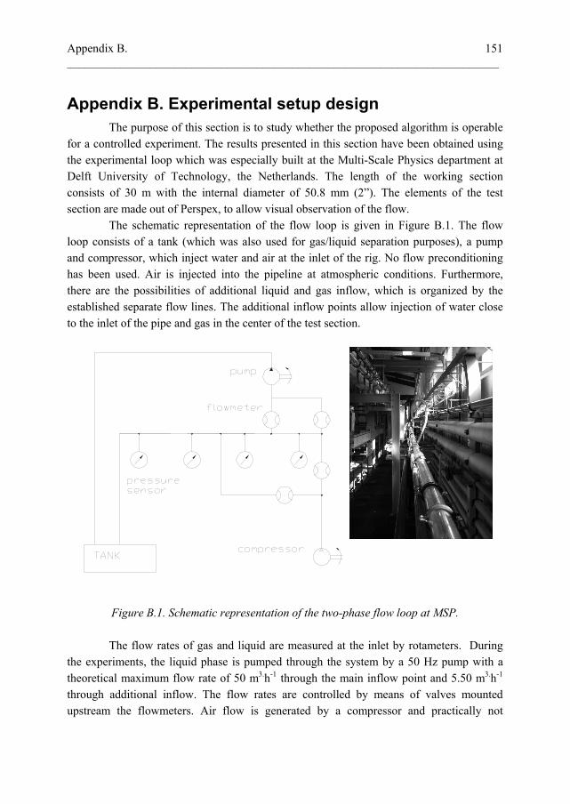
Appendix B. _________________________________________________________________________
151
Appendix B. Experimental setup design The purpose of this section is to study whether the proposed algorithm is operable for a controlled experiment. The results presented in this section have been obtained using the experimental loop which was especially built at the Multi-Scale Physics department at Delft University of Technology, the Netherlands. The length of the working section consists of 30 m with the internal diameter of 50.8 mm (2”). The elements of the test section are made out of Perspex, to allow visual observation of the flow. The schematic representation of the flow loop is given in Figure B.1. The flow loop consists of a tank (which was also used for gas/liquid separation purposes), a pump and compressor, which inject water and air at the inlet of the rig. No flow preconditioning has been used. Air is injected into the pipeline at atmospheric conditions. Furthermore, there are the possibilities of additional liquid and gas inflow, which is organized by the established separate flow lines. The additional inflow points allow injection of water close to the inlet of the pipe and gas in the center of the test section.
Figure B.1. Schematic representation of the two-phase flow loop at MSP.
The flow rates of gas and liquid are measured at the inlet by rotameters. During the experiments, the liquid phase is pumped through the system by a 50 Hz pump with a theoretical maximum flow rate of 50 m3.h-1 through the main inflow point and 5.50 m3.h-1 through additional inflow. The flow rates are controlled by means of valves mounted upstream the flowmeters. Air flow is generated by a compressor and practically not

Appendix B _____________________________________________________________ 152
restricted to any flow rate, except those prescribed by flow meter limitations. In order to be able to use the installed gas phase flow meters, some post-processing has to be made to convert the readings into the actual gas phase flow rate, since these meters are designed initially for liquid flows and have to be rescaled. Pressure transducers (DRUCK, PDCR 820) with a pressure range of 1.5 Bar were mounted at four locations of the wellbore. Two types of fluid injection have been used: the liquid is entering the wellbore at x=4.96m orthogonal to the main stream, while the gas phase enters the pipeline at x=14.84m parallel to flow. This difference can be seen in Figures B.2-B.3, where the pictures of the inflow points are given. The test section of the flow loop is sketched in detail in Figure B.4.
Figure B.4. Detailed view of horizontal test section.
Figure B.2. Liquid injection point. Figure B.3. Gas injection point.

Appendix B. _________________________________________________________________________
153
Preliminary experimental runs on two-phase flow were carried out to identify the flow regime in the operational range of setup. The working range of the superficial liquid velocity is from 1 to 4.5 m/s and superficial gas velocity from 0 to 5 m/s. The obtained range of flow conditions used is depicted in Figure B.5 where it is compared with flow regime map by Mandhane et al., 1974.
Figure B.5. Flow regime map (after Mandhane et al., 1974) with rectangular representing
the working range of the designed flow loop.
It is suggested that the designed flow loop can be used for the following purposes:
To analyze the existing flow patterns, define the flow regime map and calculate flow parameters relevant to a forward simulation of multiphase flows.
To obtain data required for multiphase model inversion, i.e. generate kinematic and dynamic waves and perform corresponding measurements.
The measurements of the pressure wave can be used to estimate the flow velocity while the static pressure drop provides the estimation of the holdup front. The latter can then be compared to a series of liquid fractions measurements, which should be available in several locations along the wellbore. The major advantage of a controlled experiment is that the model error associated with various flow phenomena can be identified and accounted separately in the estimation. The use of real experimental data may be problematic, due to numerous shortcomings of experimental work. In particular, all the flow models considered require the stable conditions within the flow loop. However, this might be difficult to achieve for certain flow regimes and flow rates. One is referred to Prickaerts, 2008 for a detailed description of preliminary work and experimental runs performed.

154

_________________________________________________________________________ 155
Afterword
From the very beginning I had doubts that I manage to write this section properly.
Should it include lengthy descriptions of all the difficulties I had, people I met, and cities I visited or better keep it for later memoirs? As things look quite different and biased from Stavanger, it didn’t work out in any formulation. Furthermore, it seems that I am just unwilling to confess that my Delft adventure is over and it is time to summarize it.
The idea of a PhD research was heavily set into my mind since 2002, when I still was a student of MSTU studying hydraulics engineering. It took me 4 years to change the main vector of my interest into the area of multiphase flows and eventually to produce a PhD thesis written in the field of applied physics. This transformation was not an easy one and first of all I want to mention Dr. Oleg Zhuravlev, who first suggested me an idea of PhD research in Delft University of Technology. Among the positions available there was only one that was somehow related to my background. Vague project proposal and natural enthusiasm: these two were the only prerequisites I had in 2006. I was able to convince Professor Rob Mudde that I have sufficient skills to start and, more important, to finish this PhD project. Rob introduced me to a world of multiphase flow and I am grateful for his guidance and help. I appreciate his critical editorial comments during preparation of this manuscript.
I will be always grateful to Annekatrien Daalmans to be patient enough to help with all the administrative problems I was facing during my stay in Delft. I wish to thank also Alberto da Costa Assafrao who became most dangerous chess opponent in Hugo de Grootstraat.
I should write down names of all people who one way or another contributed to this work and provided me an abundant social and scientific environment but this list is enormous. Therefore I would like to them all (including Russian-speaking people and colleagues from Multi-Scale Physics department). All errors are, of course, theirs.) Stavanger, January 2010

156

157
About the author
19 April, 1982 1999-2005 2004-2006 2006-2010 2010
Born in Moscow, Soviet Union
Bauman Moscow State Technical University, department of hydraulic engineering.
Contractor, Schlumberger Moscow Research, Russia
PhD research, Multiscale Physics Department, Delft University of Technology, the Netherlands
Product specialist, Roxar Flow Measurement, Stavanger, Norway

158