Compulsory Education and the Benefits of Schooling∗

Melvin Stephens Jr.

University of Michigan

and NBER

Dou-Yan Yang

Carnegie Mellon University

This Version: September 21, 2013

∗Stephens: Department of Economics, University of Michigan, 611 Tappan St., Ann Arbor, MI, 48109, e-mail:mstep@umich.edu and National Bureau of Economic Research, Cambridge, MA. Yang: Heinz College, CarnegieMellon University, 5000 Forbes Avenue, Pittsburgh, PA, 15213, e-mail: douyany@andrew.cmu.edu. We would liketo thank John Bound, Kerwin Charles, Steve Haider, and seminar participants at Columbia University, Ohio StateUniversity, the University of Kentucky, and UM-MSU-UWO Labor Day for helpful comments and suggestions. Anearlier version of this paper circulated with the title “Schooling Laws, School Quality, and the Returns to Schooling.”

Compulsory Education and the Benefits of Schooling

Abstract

Causal estimates of the benefits of increased schooling using U.S. state schooling laws as instruments

typically rely on specifications which assume common trends across states in the factors affecting

different birth cohorts. Differential changes across states during this period, such as relative school

quality improvements, suggest that this assumption may fail to hold. Across a number of outcomes

including wages, unemployment, and divorce, we find that statistically significant causal estimates

become insignificant and, in many instances, wrong-signed when allowing year of birth effects to

vary across regions.

The United States experienced a dramatic increase in educational attainment during the 20th

century. While less than 25 percent of Americans born in 1930 attended college, over 60 percent

of those born in 1970 did so (Goldin and Katz 2008). These gains were precipitated by the rapid

expansion of secondary education, known as the “High School Movement,” which resulted in the

high school graduation rate rising from 9 percent in 1910 to 51 percent in 1940 (Goldin 1998). Nu-

merous factors contributed to the spread of high schools in the first part of the century including

competition among localities to increase property values and a rising demand for educated workers

(Goldin and Katz 2008). Prior research has also found that statewide policies such as compul-

sory schooling requirements and child labor restrictions led to significant increases in educational

attainment (Lang and Kropp 1986; Acemoglu and Angrist 2000; Lleras-Muney 2002).

These state-level changes in schooling requirements are used as instrumental variables to ex-

amine the impact of increased schooling on a wide range of outcomes including wages, mortality,

incarceration, and the social returns to schooling (Acemoglu and Angrist 2000; Lochner and Moretti

2004; Lleras-Muney 2005; Oreopoulos 2006). Identification of these effects is achieved by exploiting

variation in the timing of the law changes across states over time such that different birth cohorts

within each state have different compulsory schooling requirements. Key to this identification

strategy, typically implemented in specifications that include state of birth and year of birth fixed

effects, is that all other changes which occur across states during this period are uncorrelated with

the law changes, educational improvements, and the outcomes under investigation.

Prior research suggests that such a “common trends” assumption is unlikely to hold in this

context. For example, Card and Krueger (1992a,b) find that gains in school quality, which improved

much more rapidly in the Southern states, had important effects on the adult wages of men who

were in school during this period. Bleakley (2007) finds that eradication of hookworm, which

affected 40 percent of Southern children before the intervention, improved schooling outcomes and

subsequent adult wages. Aaronson and Mazumder (2011) find that the construction of Rosenwald

schools had significant effects on the schooling attainment and cognitive test scores of rural Southern

Blacks. Thus, standard estimates of the benefits of increased schooling may be driven by a variety

of factors that had disproportionate effects across the regions of the U.S. rather than by variation

within states over time as is typically thought to identify these models.

1

In this paper, we examine the importance of the common trends assumption for estimates of the

benefits of schooling when using schooling laws as instruments. In samples commonly used in the

prior literature (the 1960-1980 U.S. Censuses) and across a number of outcomes including wages,

occupational status, unemployment, and divorce, we find statistically significant causal effects of

increased schooling when using the baseline specification which includes state of birth and year of

birth effects. However, these estimates become insignificant and, in many instances, “wrong-signed”

when using specifications in which the year of birth effects vary across the four U.S. Census regions

of birth. While our first stage estimates of the impact of schooling laws on educational attainment

are somewhat weakened by allowing regional differences in the year of birth effects, our findings are

not simply due to a weak first stage as we still find F-statistics on the excluded instruments that

substantially exceed conventional weak instrument thresholds.

Our findings indicate that results from the commonly-used baseline specification are driven

by differences between regions as opposed to variation within states over time. By using region-

specific year of birth effects, we remain agnostic as to the exact reason why the results change so

dramatically when we implement a relatively minor, but substantively important, modification to

the baseline specification. We present additional results in which we adjust the baseline specification

by adding Card and Krueger’s (1992a) school quality measures which vary at the state of birth/year

of birth level. Again we find that many of the previously significant estimates become insignificant

and/or wrong-signed suggesting that differential relative improvements in school quality across

states, which are not accounted for in the baseline specification, may be one possible explanation

for our findings.

1 Data

As with the majority of the literature which examines uses schooling laws as instruments for

estimating the benefits of schooling, we use data from the 1960-1980 U.S. Censuses of Population

(Ruggles et al. 2010). We limit our analysis to native-born individuals ages 25 to 54 across these

three Census years which encompasses the 1905 to 1954 birth cohorts. These birth cohorts comprise

a substantial subset of the birth cohorts that are typically found in studies which use compulsory

2

schooling and child labor laws as instruments.1 The evidence on the efficacy of compulsory schooling

laws is far more substantial for these cohorts than for more recent birth cohorts.2 Our analysis

focuses on Whites since we find no evidence supporting the efficacy of compulsory schooling laws

for Blacks in our sample.3 For our analysis, the demographic information that we require from

the Census is age, quarter of birth, and state of birth in order to determine both the prevailing

schooling laws and the quality of schooling that the sample members faced when growing up. Years

of schooling is measured as the highest grade completed. The log weekly wage is calculated by

dividing annual wages by weeks worked.4

1.1 Schooling Laws

Multiple aspects of state compulsory schooling laws and child labor laws are used to determine the

minimum years of school that a child is required to attend (Acemoglu and Angrist 2000; Goldin

and Katz 2003). Compulsory schooling laws specify an entry age by which the child is required to

attend school and a drop out age at which the child can choose to unconditionally stop attending

school. There are two primary types of exceptions frequently written into schooling laws that allow

children to stop attending school before the drop out age. The first type of exception allows children

to stop attending if they have completed a specified number of schooling years.5 The second type

of exception allows children to be excused from school attendance if they have secured employment

and have also reached both minimum age and years of schooling requirements. States typically

have either the first or second type of exception; only in a handful of cases do states provide both

1E.g., Lleras-Muney (2005) uses individuals born from 1900 to 1925, Lochner and Moretti (2004) use men bornin 1900 to 1960, and Oreopolous (2006) uses cohorts born in 1900 to 1961.

2See, e.g., Lleras-Muney (2002) and Goldin and Katz (2008). There has been virtually little research establishinga causal link between schooling laws and educational attainment for more recent years. Edwards (1978) finds littleevidence that, when accounting for possible endogeneity, schooling laws affected educational attainment for cohortsin school between 1940 and 1960.

3After we adjust the specification to account for differential trends across regions, we find that many of the firststage estimates of the relationship between schooling laws and educational attainment for Blacks are wrong-signedand, in some cases, statistically significant. This result holds for all of the codings of the schooling laws that weexamine. In addition, the F-statistics on the excluded instruments fall well below the conventional weak instrumentthreshold. These results are available from the authors.

4We follow Acemoglu and Angrist (2000) in the construction of the variables using the procedures discussed inthe Appendix of their paper.

5In some instances these exceptions have both minimum age and completed years of schooling requirements.

3

types of exceptions.6

Child labor laws specify the age and/or completed schooling requirement needed to be reached

in order to enter the labor force. In some instances, these laws explicitly specify the requirements

needed to work during school hours. In other situations, however, only the age at which the child

can work when school is not in session is specified (i.e., outside of school hours or during vacations).

Thus, having achieved the minimum age and/or amount of schooling needed for a work permit does

not necessarily provide an exception to the compulsory schooling law.

The compulsory schooling measures that primarily have been used in the prior literature are

the two measures coded by Acemoglu and Angrist (2000). Their first measure is based only on the

schooling attendance portion of the legal statutes. Compulsory attendance (CAst) for those born

in state s in year t is computed as

CAst = max{Dropout Agest − Enrollment Agest,Years of School Needed to Dropoutst}

where the variables used to construct the measure are those prevailing in the individual’s birth

state when they were age fourteen.7 The first quantity in the max function, the difference between

the enrollment and drop out ages, computes the minimum number of years that an individual needs

to attend school without making use of any exceptions. The second term in the max function is

years of completed schooling after which the student can drop out without working. As Goldin and

Katz (2003) have noted, since this second term in the max function is an exception which allows

the child to leave before the drop out age, the correct calculation of CA would use a min function.

We return to the implications of using the max versus the min function below.

Their second compulsory schooling measure, child labor (CLst), is based primarily on the child

labor law and is computed as

CLst = max{Work Permit Agest − Enrollment Agest,Education for Work Permitst}6There are other types of exceptions to the compulsory schooling laws which frequently include economic need

of the family, physical or mental handicap, and living too far from the nearest school. Consistent with the priorliterature, we have not coded these exceptions to the compulsory schooling law.

7They assign laws as of age fourteen since most states require students to attend through age fourteen for thebirth cohorts that they examine. Goldin and Katz use a similar approach except that they assign enrollment agebased on the laws in place at age 6.

4

The first term in the max function is the difference between the age at which the child can receive

a work permit and the age at which they must enter school. The second term is the number of

years of schooling needed to receive a work permit. A max function is appropriate in this instance

since both requirements are necessary to receive a work permit. However, as we mentioned above,

eligibility for a work permit does not necessarily exempt the child from school attendance although

in a number of instances these age and/or schooling requirements are the same.

We construct a required schooling (RSst) measure which accounts for any changes to the com-

pulsory attendance and child labor laws that may occur during the child’s school years.8 For birth

cohort t from state s, our measure is generated by iterating through ages six to seventeen to de-

termine whether the child is required to attend school at that age based in the law that is place in

that same year.9 By using this iterative process, we determine the number of years that the child

would have been required to complete by the current age. In turn, we use this cumulative amount

of required schooling to determine if the child is eligible for any school attendance exceptions at

the current age. For each age as we iterate through the child’s schooling years, if the student either

has not reached their drop out age or is not eligible for an exception, we increment the number

of required schooling years by one. Once the child either reaches their drop out age or meets the

minimum age and/or years of schooling requirements to satisfy a schooling exception, we do not

increment required schooling further unless there is a subsequent change in the schooling statutes.10

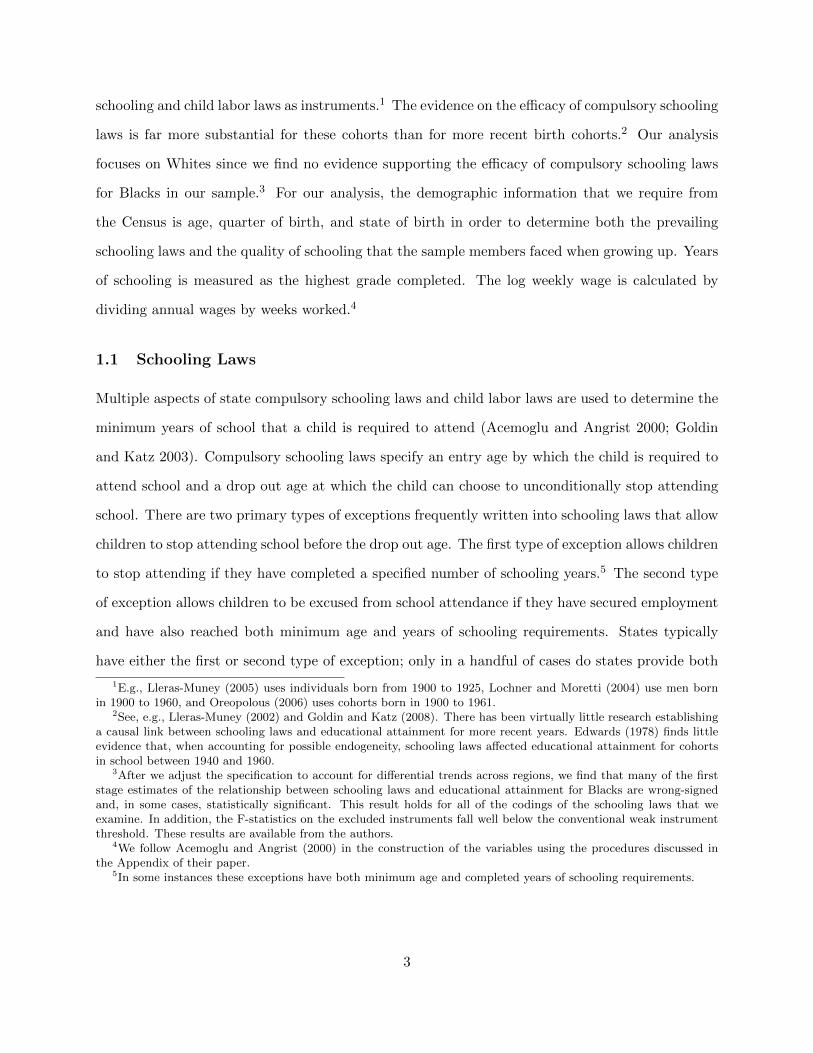
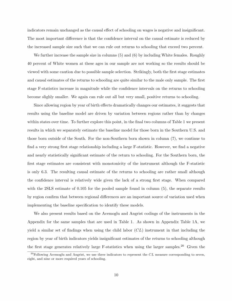
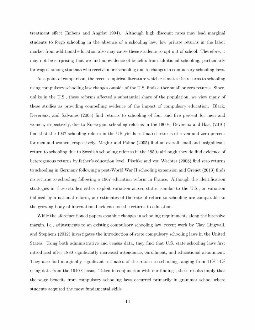
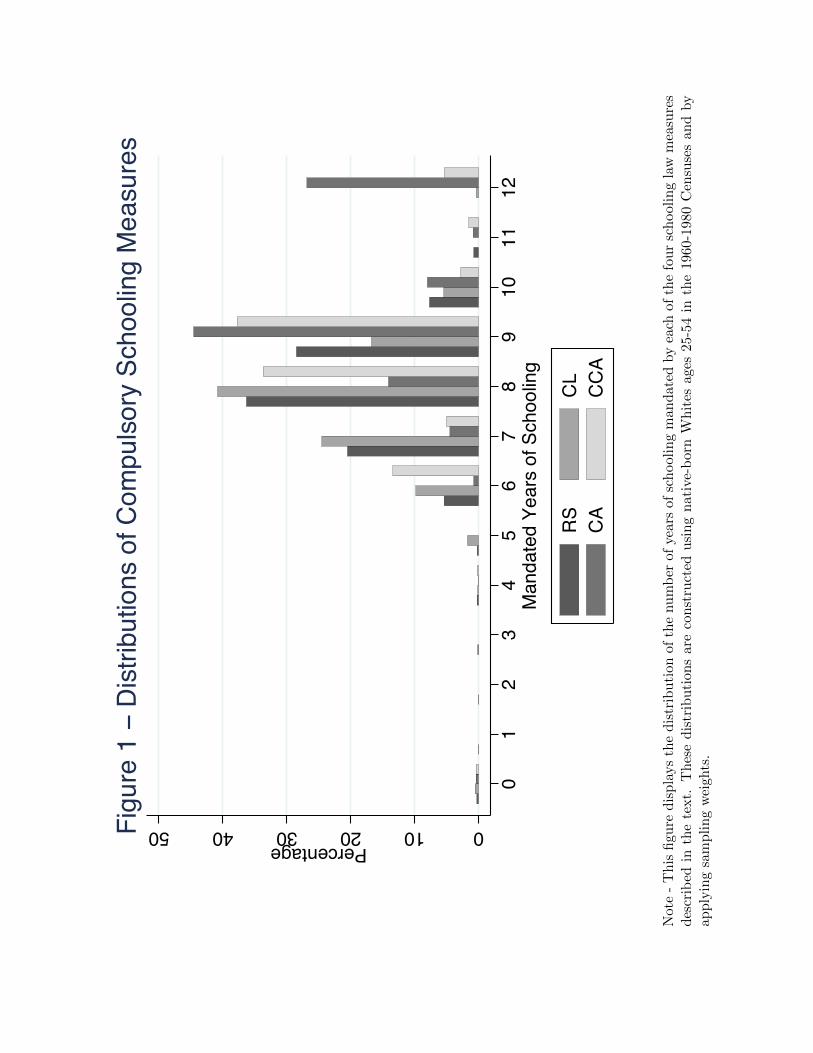
Figure 1 displays the (weighted) distributions of alternative codings of the schooling laws for

native-born Whites ages 25-54 in the 1960-1980 Censuses. The figure displays multiple histograms

for the alternative codings of the schooling laws on the same x-axis to emphasize the contrast

8Our measure also reflects additional data collection on the timing of schooling requirement changes. WhereasAcemoglu and Angrist (2000) collected data on these laws at roughly five-year intervals from secondary sources, wedetermine the exact year in which every law changed using a number of additional secondary sources as well as theoriginal legislation found in state session laws. We verify each of the changes coded by Acemoglu and Angrist andby Goldin and Katz and, when necessary, reconcile differences between the two sets of codings. A file containing theresults of these comparisons and explaining differences between our codings and those found in prior work is availablefrom the authors upon request.

9We begin at age six since there is no required entry age younger than six during this period. Similarly, the oldestthat we need to check is seventeen since the oldest drop out age in our sample is eighteen.

10As we mentioned above, the non-work schooling exceptions typically only specify a number of years of completedschooling to exemption from further attendance. In those cases in which this type of exception also has a minimumage requirement, it is nearly universally true that entry age plus the completed years of schooling equals or exceedsthe minimum age requirement. That is, the minimum ages given for these schooling exceptions are virtually neverbinding. As such, we have not separately coded these ages as is also true with previous codings (Acemoglu andAngrist 2000; Lleras-Muney 2002,2005; Goldin and Katz 2003).

5

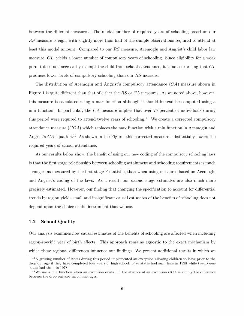
between the different measures. The modal number of required years of schooling based on our

RS measure is eight with slightly more than half of the sample observations required to attend at

least this modal amount. Compared to our RS measure, Acemoglu and Angrist’s child labor law

measure, CL, yields a lower number of compulsory years of schooling. Since eligibility for a work

permit does not necessarily exempt the child from school attendance, it is not surprising that CL

produces lower levels of compulsory schooling than our RS measure.

The distribution of Acemoglu and Angrist’s compulsory attendance (CA) measure shown in

Figure 1 is quite different than that of either the RS or CL measures. As we noted above, however,

this measure is calculated using a max function although it should instead be computed using a

min function. In particular, the CA measure implies that over 25 percent of individuals during

this period were required to attend twelve years of schooling.11 We create a corrected compulsory

attendance measure (CCA) which replaces the max function with a min function in Acemoglu and

Angrist’s CA equation.12 As shown in the Figure, this corrected measure substantially lowers the

required years of school attendance.

As our results below show, the benefit of using our new coding of the compulsory schooling laws

is that the first stage relationship between schooling attainment and schooling requirements is much

stronger, as measured by the first stage F-statistic, than when using measures based on Acemoglu

and Angrist’s coding of the laws. As a result, our second stage estimates are also much more

precisely estimated. However, our finding that changing the specification to account for differential

trends by region yields small and insignificant causal estimates of the benefits of schooling does not

depend upon the choice of the instrument that we use.

1.2 School Quality

Our analysis examines how causal estimates of the benefits of schooling are affected when including

region-specific year of birth effects. This approach remains agnostic to the exact mechanism by

which these regional differences influence our findings. We present additional results in which we

11A growing number of states during this period implemented an exception allowing children to leave prior to thedrop out age if they have completed four years of high school. Five states had such laws in 1928 while twenty-onestates had them in 1978.

12We use a min function when an exception exists. In the absence of an exception CCA is simply the differencebetween the drop out and enrollment ages.

6

investigate one potential factor, school quality. We use Card and Krueger’s (1992a) school quality

measures which they compiled from issues of the Biennial Survey of Education containing the

results of surveys of state education departments performed by the U.S. Office of Education from

1918 to 1966. Card and Krueger focus on the pupil/teacher ratio, the length of the school term,

and average teacher salaries. For each of these quality attributes, Card and Krueger create a single

measure for each state of birth/year of birth cohort by averaging the prevailing measures during

the years in which that cohort was ages six to seventeen. We follow the same aggregation procedure

for the school quality data.13 Since our oldest cohort was born in 1905, we also make use of school

quality data beginning in 1911 which is available in earlier years of the Survey.14 Furthermore,

since our youngest cohort was born in 1954, we extend their data forward in time using various

editions of the Digest of Educational Statistics.

2 Empirical Methodology

Following the prior literature, the outcome equation that we estimate using two stage least squares

(2SLS) is

Outcomest,i = αEducst,i + χs + δt + βXst,i + εst,i (1)

where Educst,i is the years of schooling of individual i born in state s in year t while χs and δt

are vectors of state of birth fixed effects and year of birth fixed effects, respectively. Depending

upon the exact sample composition, we also include a quartic in age, Census year indicators, and

an indicator for gender to this baseline specification as part of Xst,i in equation (1). To account for

the aforementioned differences in trends across states, we also present specifications in which Xst,i

contains either year of birth indicators that differ across the four U.S. Census regions of birth or

the Card and Krueger school quality measures.15

13We thank David Card and Alan Krueger for making these data available to us.14We thank Jeff Lingwall for making these data available to us. To create relative teacher wages, we also obtained

the same market wage measures from the sources found in the Appendix to Card and Krueger (1992a).15Prior papers have also included state of residence fixed effects in wage equations to account for differences in

labor market conditions across states that might affect wages (e.g., Card and Krueger (1992a,b)). Including theseregressors has very little effect on our estimates of α across the various specifications we examine. These results areavailable from the authors.

7

The corresponding first stage equation that we estimate is

Educst,i = πCSLst + λs + θt + υXst,i + νst,i (2)

where λs is a vector of state of birth fixed effects and θt is a vector of year of birth effects. CSLst

represents the schooling law instruments which, for our primary analysis, are based on our RS

measure of the required years of schooling. Since this equation includes both state of birth and

year of birth fixed effects, the coefficients on the CSLst instruments are identified by both variation

in laws across states for each birth cohort as well as variation within states across birth cohorts.

We specify the RS instrument as three indicators, RS7, RS8, and RS9, corresponding to being

required to attend seven, eight, and nine or more years of schooling, respectively. We also present

results based on Acemoglu and Angrist’s child labor measure (CL) and the corrected version of

their compulsory attendance measure (CCA).

As is well-known, applying 2SLS with weak instruments will not only yield biased point esti-

mates, but the standard 2SLS confidence intervals are incorrect (Nelson and Startz 1990; Stock

and Staiger 1997). For the majority of our analysis, the first stage statistics are well above the

conventional weak instrument thresholds. As such, we only present the 2SLS estimates below.16

To be conservative with our inferences, we implement Moreira’s (2003) conditional likelihood ratio

(CLR) test which is “nearly” optimal among methods to construct confidence intervals when us-

ing weak instruments under the assumption that the model has i.i.d. normally distributed errors

(Andrews, Moreira, and Stock 2007).17 However, studies using schooling law instruments typically

assume that the error terms are correlated among those born in the same state of birth/year of

birth cell. Thus, we report CLR confidence intervals that allow for clustering using the methods

discussed in Finlay and Magnusson (2009).18

16The point estimates from using limited information maximum likelihood (LIML), which are available from theauthors, are very similar to the 2SLS estimates shown below.

17Alternative approaches for constructing confidence intervals with weak instruments include the Anderson-Rubinstatistic (Anderson and Rubin 1949) and a Lagrange multiplier statistic (Kleibergen 2002).

18The CLR confidence intervals are computing using version 1.0.7 of the -rivtest- command for Stata (Finlay andMagnusson 2009). This command also allows for the use of inverse probability weights which are required since thesampling rate for publicly available Census varies over time: the 1960 Census is a 1 in 100 sample, the 1970 is 1 in 50,the 1980 is 1 in 20. We find similar confidence intervals when we calculate Kleibergen’s (2002) Lagrange Multipliertest and allow for clustering and sampling weights (Finlay and Magnusson 2009). Results using this alternative

8

3 Results

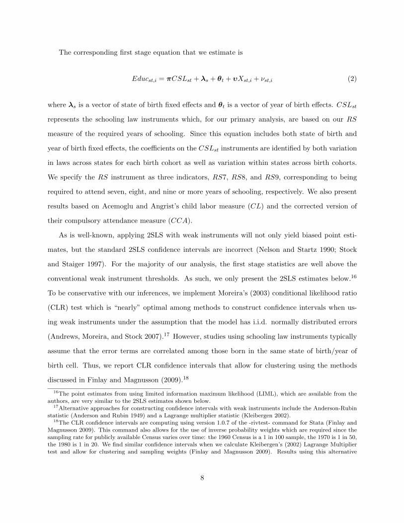
3.1 The Impact of Schooling on Wages

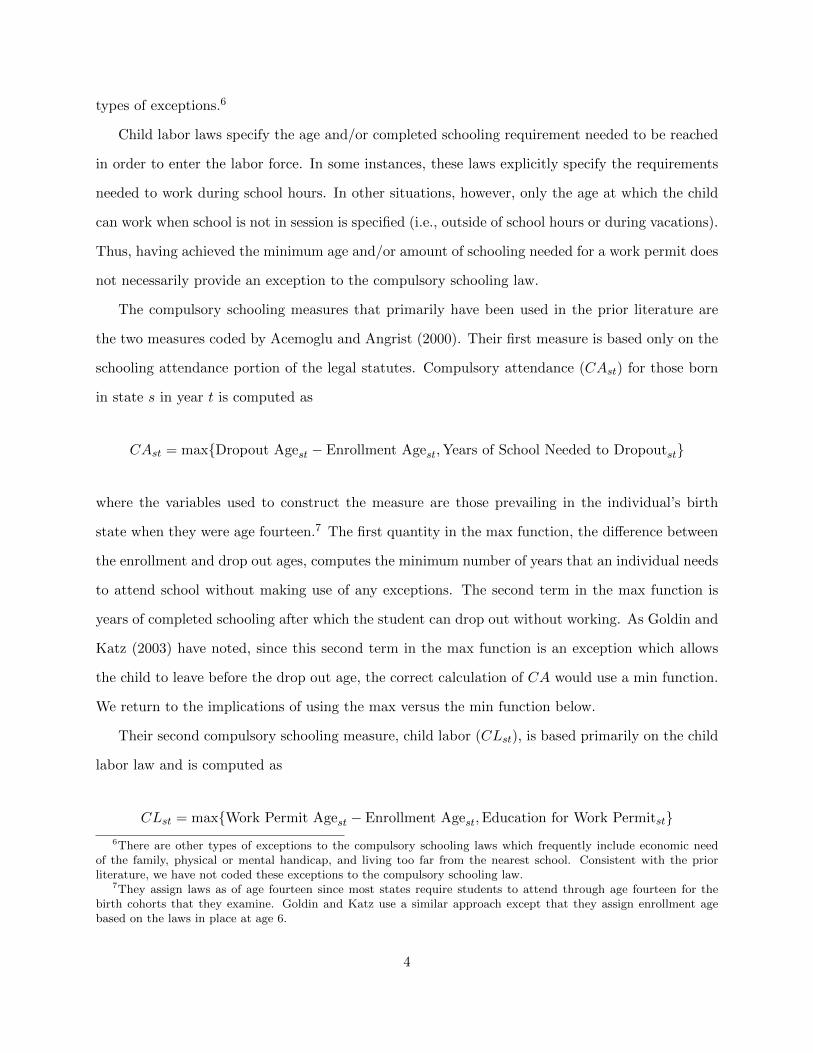
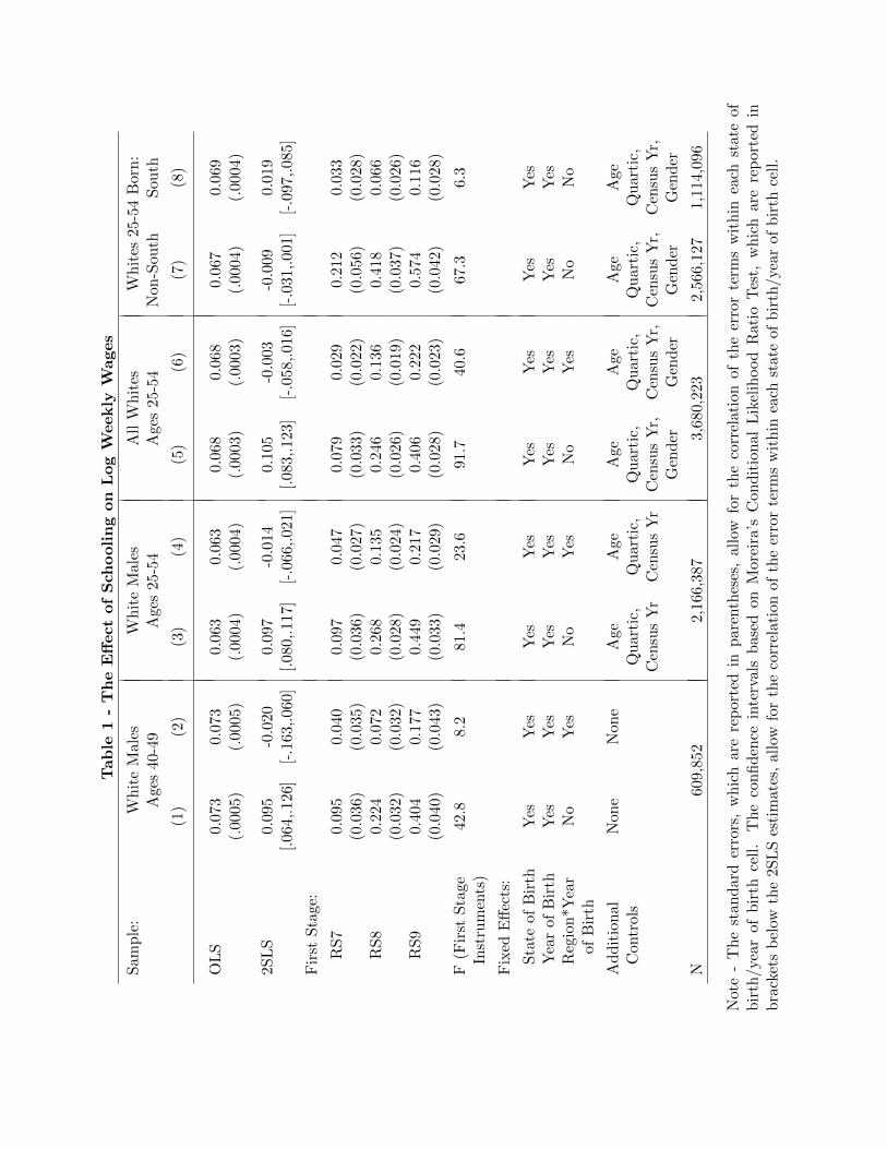
We limit our analysis in Table 1 to examining the causal effect of schooling on log weekly wages

in order to focus on how the first stage estimates are affected by changing the model specification

and the sample composition. The results shown in columns (1) and (2) of the Table limit the

sample to Acemoglu and Angrist’s (2000) primary sample of White males ages 40-49 from the

1960-1980 Censuses of Population.19 The Table presents standard errors below their corresponding

point estimates throughout except for the 2SLS estimates below which we report the 95 percent

confidence intervals based on Moreira’s CLR test. Column (1) shows that both the OLS and 2SLS

estimates of the returns to schooling are statistically significant and of the usual magnitudes. The

first stage F-statistic exceeds 42, well above the conventional weak instrument threshold of 10,

while the first stage point estimates are consistent with monotonicity of the instrument because

increases in the required years of schooling correspond to higher levels of schooling attainment.

Allowing for differential trends through the inclusion of region by year of birth indicators dra-

matically alters the causal estimates of the returns to schooling. As shown in column (2) of Table 1,

these estimates becomes negative in sign and statistically insignificant. The first stage estimates fall

in magnitude although they remain consistent with monotonicity of the instrument and are jointly

significant with an F-statistic of 8.2. Corresponding to the reduction in the F-statistic, the CLR

confidence interval is much larger than in column (1) and, although the estimate is insignificant,

we are unable to rule out a rate of return to schooling of six percent.

Given the reduced precision of the estimate due to the inclusion of region by year of birth

indicators, we next increase the sample to include all White males between ages 25-54 in columns

(3) and (4). Doing so dramatically increases the first stage F-statistics to 81.4 and 23.6, respectively,

while the first stage estimates on the instruments remain very comparable in magnitude to those

found in the first two columns. Moreover, the implications from including the region by year of birth

method of computing the confidence intervals are available from the authors.19We are able to exactly re-create their dataset and results based on the code they provide on-line. The original

dataset is available on-line at http://econ-www.mit.edu/faculty/angrist/data1/data/aceang00. This sample corre-sponds to the 1910-1939 birth cohorts.

9

indicators remain unchanged as the causal effect of schooling on wages is negative and insignificant.

The most important difference is that the confidence interval on the causal estimate is reduced by

the increased sample size such that we can rule out returns to schooling that exceed two percent.

We further increase the sample size in columns (5) and (6) by including White females. Roughly

40 percent of White women at these ages in our sample are not working so the results should be

viewed with some caution due to possible sample selection. Strikingly, both the first stage estimates

and causal estimates of the returns to schooling are quite similar to the male only sample. The first

stage F-statistics increase in magnitude while the confidence intervals on the returns to schooling

become slighly smaller. We again can rule out all but very small, positive returns to schooling.

Since allowing region by year of birth effects dramatically changes our estimates, it suggests that

results using the baseline model are driven by variation between regions rather than by changes

within states over time. To further explore this point, in the final two columns of Table 1 we present

results in which we separately estimate the baseline model for those born in the Southern U.S. and

those born outside of the South. For the non-Southern born shown in column (7), we continue to

find a very strong first stage relationship including a large F-statistic. However, we find a negative

and nearly statistically significant estimate of the return to schooling. For the Southern born, the

first stage estimates are consistent with monotonicity of the instrument although the F-statistic

is only 6.3. The resulting causal estimate of the returns to schooling are rather small although

the confidence interval is relatively wide given the lack of a strong first stage. When compared

with the 2SLS estimate of 0.105 for the pooled sample found in column (5), the separate results

by region confirm that between regional differences are an important source of variation used when

implementing the baseline specification to identify these models.

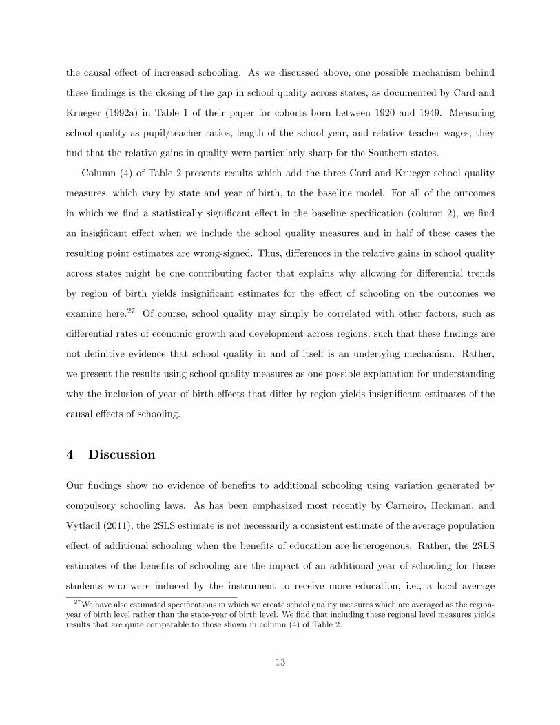
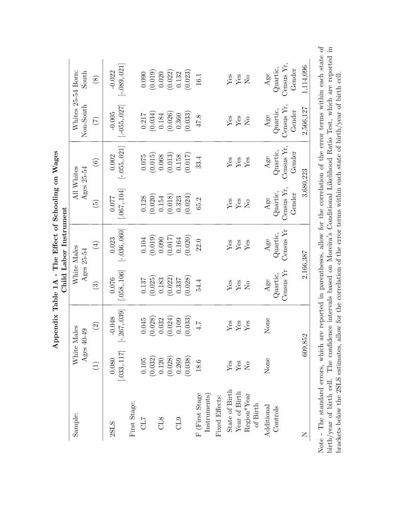
We also present results based on the Acemoglu and Angrist codings of the instruments in the

Appendix for the same samples that are used in Table 1. As shown in Appendix Table 1A, we

yield a similar set of findings when using the child labor (CL) instrument in that including the

region by year of birth indicators yields insignificant estimates of the returns to schooling although

the first stage generates relatively large F-statistics when using the larger samples.20 Given the

20Following Acemoglu and Angrist, we use three indicators to represent the CL measure corresponding to seven,eight, and nine or more required years of schooling.

10

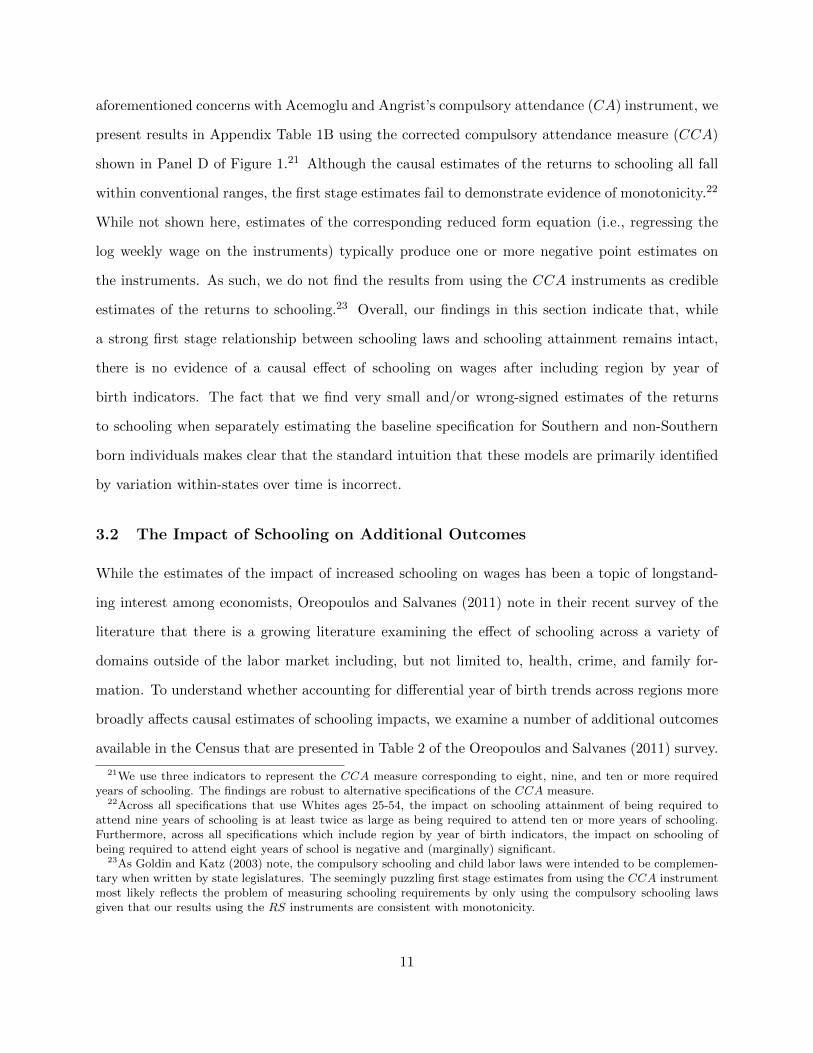
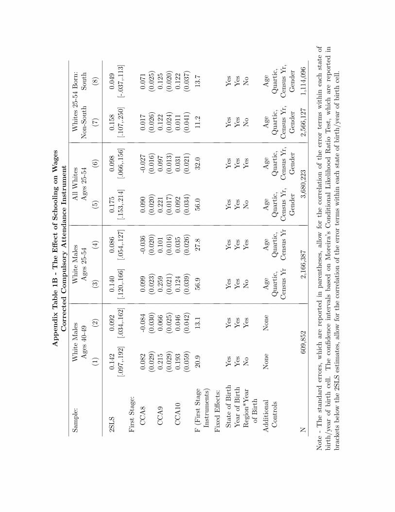
aforementioned concerns with Acemoglu and Angrist’s compulsory attendance (CA) instrument, we

present results in Appendix Table 1B using the corrected compulsory attendance measure (CCA)

shown in Panel D of Figure 1.21 Although the causal estimates of the returns to schooling all fall

within conventional ranges, the first stage estimates fail to demonstrate evidence of monotonicity.22

While not shown here, estimates of the corresponding reduced form equation (i.e., regressing the

log weekly wage on the instruments) typically produce one or more negative point estimates on

the instruments. As such, we do not find the results from using the CCA instruments as credible

estimates of the returns to schooling.23 Overall, our findings in this section indicate that, while

a strong first stage relationship between schooling laws and schooling attainment remains intact,

there is no evidence of a causal effect of schooling on wages after including region by year of

birth indicators. The fact that we find very small and/or wrong-signed estimates of the returns

to schooling when separately estimating the baseline specification for Southern and non-Southern

born individuals makes clear that the standard intuition that these models are primarily identified

by variation within-states over time is incorrect.

3.2 The Impact of Schooling on Additional Outcomes

While the estimates of the impact of increased schooling on wages has been a topic of longstand-

ing interest among economists, Oreopoulos and Salvanes (2011) note in their recent survey of the

literature that there is a growing literature examining the effect of schooling across a variety of

domains outside of the labor market including, but not limited to, health, crime, and family for-

mation. To understand whether accounting for differential year of birth trends across regions more

broadly affects causal estimates of schooling impacts, we examine a number of additional outcomes

available in the Census that are presented in Table 2 of the Oreopoulos and Salvanes (2011) survey.

21We use three indicators to represent the CCA measure corresponding to eight, nine, and ten or more requiredyears of schooling. The findings are robust to alternative specifications of the CCA measure.

22Across all specifications that use Whites ages 25-54, the impact on schooling attainment of being required toattend nine years of schooling is at least twice as large as being required to attend ten or more years of schooling.Furthermore, across all specifications which include region by year of birth indicators, the impact on schooling ofbeing required to attend eight years of school is negative and (marginally) significant.

23As Goldin and Katz (2003) note, the compulsory schooling and child labor laws were intended to be complemen-tary when written by state legislatures. The seemingly puzzling first stage estimates from using the CCA instrumentmost likely reflects the problem of measuring schooling requirements by only using the compulsory schooling lawsgiven that our results using the RS instruments are consistent with monotonicity.

11

Furthermore, we present results separately for males and females since we examine multiple labor

market outcomes and roughly 40 percent of women in our sample are not in the labor force.24

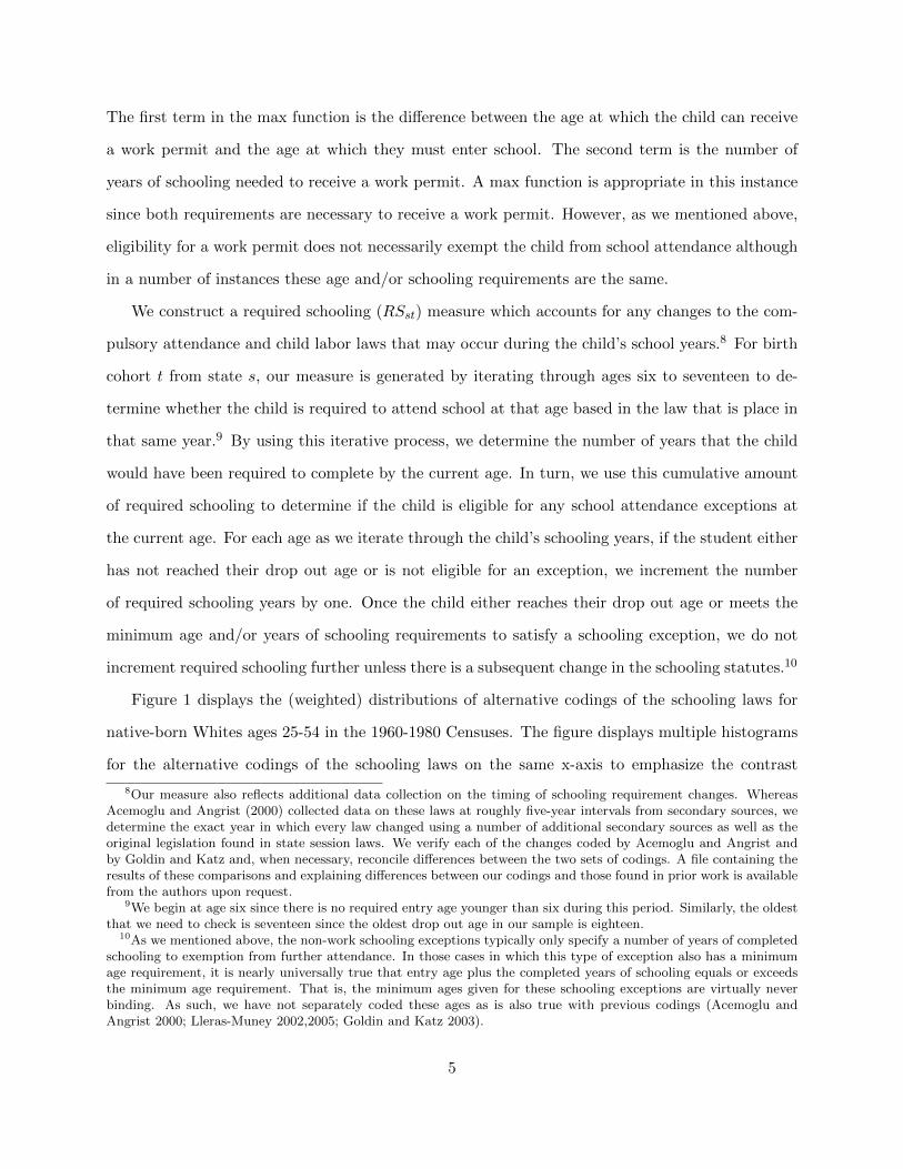
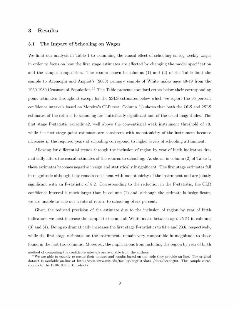
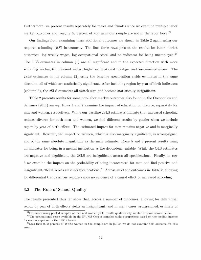
Our findings from examining these additional outcomes are shown in Table 2 again using our

required schooling (RS) instrument. The first three rows present the results for labor market

outcomes: log weekly wages, log occupational score, and an indicator for being unemployed.25

The OLS estimates in column (1) are all significant and in the expected direction with more

schooling leading to increased wages, higher occupational prestige, and less unemployment. The

2SLS estimates in the column (2) using the baseline specification yields estimates in the same

direction, all of which are statistically significant. After including region by year of birth indicators

(column 3), the 2SLS estimates all switch sign and become statistically insignificant.

Table 2 presents results for some non-labor market outcomes also found in the Oreopoulos and

Salvanes (2011) survey. Rows 4 and 7 examine the impact of education on divorce, separately for

men and women, respectively. While our baseline 2SLS estimates indicate that increased schooling

reduces divorce for both men and women, we find different results by gender when we include

region by year of birth effects. The estimated impact for men remains negative and is marginally

significant. However, the impact on women, which is also marginally significant, is wrong-signed

and of the same absolute magntitude as the male estimate. Rows 5 and 8 present results using

an indicator for being in a mental institution as the dependent variable. While the OLS estimates

are negative and significant, the 2SLS are insignificant across all specifications. Finally, in row

6 we examine the impact on the probability of being incarcerated for men and find positive and

insignificant effects across all 2SLS specifications.26 Across all of the outcomes in Table 2, allowing

for differential trends across regions yields no evidence of a causal effect of increased schooling.

3.3 The Role of School Quality

The results presented thus far show that, across a number of outcomes, allowing for differential

region by year of birth effects yields an insignificant, and in many cases wrong-signed, estimate of

24Estimates using pooled samples of men and women yield results qualitatively similar to those shown below.25The occupational score available in the IPUMS Census samples ranks occupations based on the median income

for each occupation in the 1950 Census.26Less than 0.02 percent of White women in the sample are in jail so we do not examine this outcome for this

group.

12

the causal effect of increased schooling. As we discussed above, one possible mechanism behind

these findings is the closing of the gap in school quality across states, as documented by Card and

Krueger (1992a) in Table 1 of their paper for cohorts born between 1920 and 1949. Measuring

school quality as pupil/teacher ratios, length of the school year, and relative teacher wages, they

find that the relative gains in quality were particularly sharp for the Southern states.

Column (4) of Table 2 presents results which add the three Card and Krueger school quality

measures, which vary by state and year of birth, to the baseline model. For all of the outcomes

in which we find a statistically significant effect in the baseline specification (column 2), we find

an insigificant effect when we include the school quality measures and in half of these cases the

resulting point estimates are wrong-signed. Thus, differences in the relative gains in school quality

across states might be one contributing factor that explains why allowing for differential trends

by region of birth yields insignificant estimates for the effect of schooling on the outcomes we

examine here.27 Of course, school quality may simply be correlated with other factors, such as

differential rates of economic growth and development across regions, such that these findings are

not definitive evidence that school quality in and of itself is an underlying mechanism. Rather,

we present the results using school quality measures as one possible explanation for understanding

why the inclusion of year of birth effects that differ by region yields insignificant estimates of the

causal effects of schooling.

4 Discussion

Our findings show no evidence of benefits to additional schooling using variation generated by

compulsory schooling laws. As has been emphasized most recently by Carneiro, Heckman, and

Vytlacil (2011), the 2SLS estimate is not necessarily a consistent estimate of the average population

effect of additional schooling when the benefits of education are heterogenous. Rather, the 2SLS

estimates of the benefits of schooling are the impact of an additional year of schooling for those

students who were induced by the instrument to receive more education, i.e., a local average

27We have also estimated specifications in which we create school quality measures which are averaged as the region-year of birth level rather than the state-year of birth level. We find that including these regional level measures yieldsresults that are quite comparable to those shown in column (4) of Table 2.

13

treatment effect (Imbens and Angrist 1994). Although high discount rates may lead marginal

students to forgo schooling in the absence of a schooling law, low private returns in the labor

market from additional education also may cause these students to opt out of school. Therefore, it

may not be surprising that we find no evidence of benefits from additional schooling, particularly

for wages, among students who receive more schooling due to changes in compulsory schooling laws.

As a point of comparison, the recent empirical literature which estimates the returns to schooling

using compulsory schooling law changes outside of the U.S. finds either small or zero returns. Since,

unlike in the U.S., these reforms affected a substantial share of the population, we view many of

these studies as providing compelling evidence of the impact of compulsory education. Black,

Devereux, and Salvanes (2005) find returns to schooling of four and five percent for men and

women, respectively, due to Norwegian schooling reforms in the 1960s. Devereux and Hart (2010)

find that the 1947 schooling reform in the UK yields estimated returns of seven and zero percent

for men and women, respectively. Meghir and Palme (2005) find an overall small and insignificant

return to schooling due to Swedish schooling reforms in the 1950s although they do find evidence of

heterogenous returns by father’s education level. Pischke and von Wachter (2008) find zero returns

to schooling in Germany following a post-World War II schooling expansion and Grenet (2013) finds

no returns to schooling following a 1967 education reform in France. Although the identification

strategies in these studies either exploit variation across states, similar to the U.S., or variation

induced by a national reform, our estimates of the rate of return to schooling are comparable to

the growing body of international evidence on the returns to education.

While the aforementioned papers examine changes in schooling requirements along the intensive

margin, i.e., adjustments to an existing compulsory schooling law, recent work by Clay, Lingwall,

and Stephens (2012) investigates the introduction of state compulsory schooling laws in the United

States. Using both administrative and census data, they find that U.S. state schooling laws first

introduced after 1880 significantly increased attendance, enrollment, and educational attainment.

They also find marginally significant estimates of the return to schooling ranging from 11%-14%

using data from the 1940 Census. Taken in conjunction with our findings, these results imply that

the wage benefits from compulsory schooling laws occurred primarily in grammar school where

students acquired the most fundamental skills.

14

As Oreopoulos and Salvanes (2011) highlight, the use of schooling law changes as instruments

for educational attainment has been extended into a number of domains outside of the labor force,

several of which that are beyond the scope of this paper. For example, recent papers examining the

health impacts of increased schooling find significant effects in the U.S. (Lleras-Muney 2005) but no

evidence of benefits in the UK (Clark and Royer, Forthcoming). In fact, Lleras-Muney does indeed

account for region by year of birth effects in her analysis. Our findings suggest that future research

using U.S. schooling law reforms should carefully account for the differential changes occuring

across the U.S. during this period with school quality being but one of many possible confounding

factors. At the very least, given the dramatically different results generated by estimating the

models separately by Census region, these studies should investigate whether their findings are

robust to comparable sample splits.

15

References

Aaronson, Daniel and Bhashkar Mazumder. 2011. “The Impact of Rosenwald Schools on

Black Achievement, Journal of Political Economy, 119(5): 821-888.

Acemoglu, Daron and Joshua Angrist. 2000. “How Large are Human-Capital Externalities?

Evidence from Compulsory-Schooling Laws,” in NBER Macroeconomics Annual 2000, Volume

15, 9-74.

Anderson, T. W. and H. Rubin. 1949. “Estimators of the Parameters of a Single Equation in

a Complete Set of Stochastic Equations,” Annals of Mathematical Statistics, 21, 570-582.

Andrews, Donald W. K., Marcelo J. Moreira, and James H. Stock. 2007. “Performance

of Conditional Wald Tests in IV Regression with Weak Instruments,” Journal of Econometrics,

139(1):116-132.

Black, Sandra E., Paul J. Devereux, and Kjell G. Salvanes. 2005. “Why the Apple

Doesn’t Fall Far: Understanding Intergenerational Transmission of Human Capital,” American

Economic Review, 95(1):437-449.

Bleakley, C. Hoyt. 2007. “Disease and Development: Evidence from Hookworm Eradication in

the American South” Quarterly Journal of Economics, February 2007, 122(1):73-117.

Card, David and Alan B. Krueger. 1992a. “Does School Quality Matter? Returns to Ed-

ucation and the Characteristics of Public Schools in the United States,” Journal of Political

Economy, 100(1):1-40.

Card, David and Alan B. Krueger. 1992b. “School Quality and Black-White Relative Earn-

ings: A Direct Assessment,” The Quarterly Journal of Economics, 107(1):151-200.

Carneiro, Pedro, James J. Heckman, and Edward J. Vytlacil. 2011. “Estimating Marginal

Returns to Education,” American Economic Review, 101(6):2754-81.

Clark, Damon and Heather Royer. Forthcoming. “The Effect of Education on Adult Mortality

and Health: Evidence from Britain,” American Economic Review.

Clay, Karen, Jeff Lingwall, and Melvin Stephens Jr. 2012. “Do Schooling Laws Matter?

Evidence from the Introduction of Compulsory Attendance Laws in the United States,” National

Bureau of Economic Research Working Paper No. 18477.

16

Devereux, Paul J. and Robert A. Hart. 2010. “Forced to be Rich? Returns to Compulsory

Schooling in Britain,” Economic Journal, 120(549):1345-1364.

Edwards, Linda Nasif. 1978. “An Empirical Analysis of Compulsory Schooling Legislation,

1940-1960,” Journal of Law and Economics, 21(1):203-222.

Finlay, Keith and Leandro Magnusson. 2009. “Implementing Weak Instrument Robust Tests

for a General Class of Instrumental Variables Models,” Stata Journal, 9(3):1-24.

Goldin, Claudia. 1998. “America’s Graduation from High School: The Evolution and Spread of

Secondary Schooling in the Twentieth Century,” Journal of Economic History, 58(2):345-374.

Goldin, Claudia and Lawrence Katz. 2003. “Mass Secondary Schooling and the State,”

National Bureau of Economic Research Working Paper No. 10075.

Goldin, Claudia and Lawrence Katz. 2008. The Race between Education and Technology,

Cambridge, MA: The Belknap Press of Harvard University Press.

Grenet, Julien. 2013. “Is it Enough to Increase Compulsory Education to Raise Earnings?

Evidence from French and British Compulsory Schooling Laws?” The Scandinavian Journal of

Economics, 115(1):176-210.

Imbens, Guido W. and Joshua D. Angrist. 1994. “Identification and Estimation of Local

Average Treatment Effects,” Econometrica, 62(2):467-475.

Kleibergen, Frank. 2002. “Pivotal Statistics for Testing Structural Parameters in Instrumental

Variables Regression,” Econometrica, 70(5):1781-1803.

Lang, Kevin and David Kropp. 1986. “Human Capital Versus Sorting: The Effects of Com-

pulsory Attendance Laws,” The Quarterly Journal of Economics, 101(3):609-624.

Lleras-Muney, Adriana. 2002. “Were Compulsory Education and Child Labor Laws Effective?

An Analysis from 1915 to 1939 in the U.S.,” Journal of Law and Economics, 45(2):401-435.

Lleras-Muney, Adriana. 2005. “The Relationship between Education and Adult Mortality in

the United States,” Review of Economic Studies, 72(1):189-221.

Lochner, Lance and Enrico Moretti. 2004. “The Effect of Education on Crime: Evidence

from Prison Inmates, Arrests, and Self-Reports,” American Economic Review, 94(1):155-189.

Meghir, Costas and Martin Palme. 2005. “Educational Reform, Ability and Parental Back-

ground,” American Economic Review, 2005, 95(1):414-424.

17

Moreira, Marcelo J. 2003. “A Conditional Likelihood Ratio Test for Structural Models,” Econo-

metrica, 71(4):1027-1048.

Nelson, Charles R. and Richard Startz. 1990. “Some Further Results on the Exact Small

Sample Properties of the Instrumental Variable Estimator,” Econometrica, 58(4):967-976.

Oreopoulos, Philip. 2006. “Estimating Average and Local Average Treatment Effects of Educa-

tion when Compulsory Schooling Laws Really Matter,” American Economic Review, 96(1):152-

175.

Oreopoulos, Philip and Kjell G. Salvanes. 2011. “Priceless: The Nonpecuniary Benefits of

Schooling,” Journal of Economic Perspectives 25(1):159-184.

Pischke, Jorn-Steffen and Till von Wachter. 2008. “Zero Returns to Compulsory Schooling

in Germany: Evidence and Interpretation,” Review of Economics and Statistics 90(3):592-598.

Ruggles, Steven, J. Trent Alexander, Katie Genadek, Ronald Goeken, Matthew B.

Schroeder, and Matthew Sobek. 2010. Integrated Public Use Microdata Series: Version

5.0 [Machine-readable database]. Minneapolis: University of Minnesota.

Staiger, Douglas and James H. Stock. 1997. “Instrumental Variables Regression with Weak

Instruments,” Econometrica, 65(3):557-586.

18

Tab

le1

-T

he

Eff

ect

of

Sch

oolin

gon

Log

Weekly

Wages

Sam

ple

:W

hit

eM

ale

sW

hit

eM

ales

All

Wh

ites

Wh

ites

25-5

4B

orn

:A

ges

40-

49A

ges

25-5

4A

ges

25-5

4N

on-S

outh

Sou

th

(1)

(2)

(3)

(4)

(5)

(6)

(7)

(8)

OL

S0.0

730.

073

0.06

30.

063

0.06

80.

068

0.06

70.

069

(.000

5)(.

000

5)(.

0004

)(.

0004

)(.

0003

)(.

0003

)(.

0004

)(.

0004

)

2S

LS

0.0

95-0

.020

0.09

7-0

.014

0.10

5-0

.003

-0.0

090.

019

[.06

4,.1

26]

[-.1

63,

.060

][.

080,

.117

][-

.066

,.02

1][.

083,

.123

][-

.058

,.01

6][-

.031

,.00

1][-

.097

,.08

5]

Fir

stS

tage:

RS

70.0

950.

040

0.09

70.

047

0.07

90.

029

0.21

20.

033

(0.0

36)

(0.0

35)

(0.0

36)

(0.0

27)

(0.0

33)

(0.0

22)

(0.0

56)

(0.0

28)

RS

80.

224

0.0

720.

268

0.13

50.

246

0.13

60.

418

0.06

6(0

.032)

(0.0

32)

(0.0

28)

(0.0

24)

(0.0

26)

(0.0

19)

(0.0

37)

(0.0

26)

RS

90.

404

0.1

770.

449

0.21

70.

406

0.22

20.

574

0.11

6(0

.040)

(0.0

43)

(0.0

33)

(0.0

29)

(0.0

28)

(0.0

23)

(0.0

42)

(0.0

28)

F(F

irst

Sta

ge42

.88.

281

.423

.691

.740

.667

.36.

3In

stru

men

ts)

Fix

edE

ffec

ts:

Sta

teof

Bir

thY

esY

esY

esY

esY

esY

esY

esY

esY

ear

of

Bir

thY

esY

esY

esY

esY

esY

esY

esY

esR

egio

n*Y

ear

No

Yes

No

Yes

No

Yes

No

No

of

Bir

th

Ad

dit

ion

alN

on

eN

one

Age

Age

Age

Age

Age

Age

Con

trols

Qu

arti

c,Q

uar

tic,

Qu

arti

c,Q

uar

tic,

Qu

arti

c,Q

uar

tic,

Cen

sus

Yr

Cen

sus

Yr

Cen

sus

Yr,

Cen

sus

Yr,

Cen

sus

Yr,

Cen

sus

Yr,

Gen

der

Gen

der

Gen

der

Gen

der

N609

,852

2,16

6,38

73,

680,

223

2,56

6,12

71,

114,

096

Not

e-

Th

est

and

ard

erro

rs,

wh

ich

are

rep

orte

din

par

enth

eses

,al

low

for

the

corr

elat

ion

ofth

eer

ror

term

sw

ith

inea

chst

ate

ofb

irth

/yea

rof

bir

thce

ll.

Th

eco

nfi

den

cein

terv

als

bas

edon

Mor

eira

’sC

ond

itio

nal

Lik

elih

ood

Rat

ioT

est,

wh

ich

are

rep

orte

din

bra

cket

sb

elow

the

2S

LS

esti

mat

es,

allo

wfo

rth

eco

rrel

atio

nof

the

erro

rte

rms

wit

hin

each

stat

eof

bir

th/y

ear

ofb

irth

cell

.

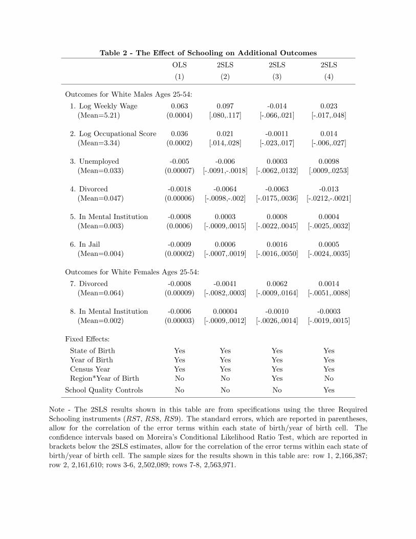
Table 2 - The Effect of Schooling on Additional Outcomes

OLS 2SLS 2SLS 2SLS

(1) (2) (3) (4)

Outcomes for White Males Ages 25-54:

1. Log Weekly Wage 0.063 0.097 -0.014 0.023(Mean=5.21) (0.0004) [.080,.117] [-.066,.021] [-.017,.048]

2. Log Occupational Score 0.036 0.021 -0.0011 0.014(Mean=3.34) (0.0002) [.014,.028] [-.023,.017] [-.006,.027]

3. Unemployed -0.005 -0.006 0.0003 0.0098(Mean=0.033) (0.00007) [-.0091,-.0018] [-.0062,.0132] [.0009,.0253]

4. Divorced -0.0018 -0.0064 -0.0063 -0.013(Mean=0.047) (0.00006) [-.0098,-.002] [-.0175,.0036] [-.0212,-.0021]

5. In Mental Institution -0.0008 0.0003 0.0008 0.0004(Mean=0.003) (0.0006) [-.0009,.0015] [-.0022,.0045] [-.0025,.0032]

6. In Jail -0.0009 0.0006 0.0016 0.0005(Mean=0.004) (0.00002) [-.0007,.0019] [-.0016,.0050] [-.0024,.0035]

Outcomes for White Females Ages 25-54:

7. Divorced -0.0008 -0.0041 0.0062 0.0014(Mean=0.064) (0.00009) [-.0082,.0003] [-.0009,.0164] [-.0051,.0088]

8. In Mental Institution -0.0006 0.00004 -0.0010 -0.0003(Mean=0.002) (0.00003) [-.0009,.0012] [-.0026,.0014] [-.0019,.0015]

Fixed Effects:

State of Birth Yes Yes Yes YesYear of Birth Yes Yes Yes YesCensus Year Yes Yes Yes YesRegion*Year of Birth No No Yes No

School Quality Controls No No No Yes

Note - The 2SLS results shown in this table are from specifications using the three RequiredSchooling instruments (RS7, RS8, RS9). The standard errors, which are reported in parentheses,allow for the correlation of the error terms within each state of birth/year of birth cell. Theconfidence intervals based on Moreira’s Conditional Likelihood Ratio Test, which are reported inbrackets below the 2SLS estimates, allow for the correlation of the error terms within each state ofbirth/year of birth cell. The sample sizes for the results shown in this table are: row 1, 2,166,387;row 2, 2,161,610; rows 3-6, 2,502,089; rows 7-8, 2,563,971.

Ap

pen

dix

Tab

le1A

-T

he

Eff

ect

of

Sch

oolin

gon

Wages

Ch

ild

Lab

or

Inst

rum

ent

Sam

ple

:W

hit

eM

ale

sW

hit

eM

ales

All

Wh

ites

Wh

ites

25-5

4B

orn

:A

ges

40-

49A

ges

25-5

4A

ges

25-5

4N

on-S

outh

Sou

th

(1)

(2)

(3)

(4)

(5)

(6)

(7)

(8)

2S

LS

0.0

80-0

.048

0.07

60.

023

0.07

70.

002

-0.0

05-0

.022

[.03

3,.1

17]

[-.2

67,

.039

][.

058,

.106

][-

.036

,.06

0][.

067,

.104

][-

.055

,.02

1][.

-055

,.02

7][-

.089

,.02

1]

Fir

stS

tage:

CL

70.

105

0.0

450.

137

0.10

40.

128

0.07

50.

217

0.09

0(0

.032)

(0.0

28)

(0.0

25)

(0.0

19)

(0.0

20)

(0.0

15)

(0.0

34)

(0.0

19)

CL

80.

120

0.0

320.

183

0.09

00.

154

0.06

80.

184

0.02

0(0

.028)

(0.0

24)

(0.0

22)

(0.0

17)

(0.0

18)

(0.0

13)

(0.0

26)

(0.0

22)

CL

90.

269

0.1

090.

337

0.16

40.

323

0.15

80.

360

0.13

2(0

.038)

(0.0

33)

(0.0

28)

(0.0

20)

(0.0

24)

(0.0

17)

(0.0

33)

(0.0

23)

F(F

irst

Sta

ge18

.64.

754

.422

.065

.233

.447

.816

.1In

stru

men

ts)

Fix

edE

ffec

ts:

Sta

teof

Bir

thY

esY

esY

esY

esY

esY

esY

esY

esY

ear

of

Bir

thY

esY

esY

esY

esY

esY

esY

esY

esR

egio

n*Y

ear

No

Yes

No

Yes

No

Yes

No

No

of

Bir

th

Ad

dit

ion

alN

on

eN

one

Age

Age

Age

Age

Age

Age

Con

trols

Qu

arti

c,Q

uar

tic,

Qu

arti

c,Q

uar

tic,

Qu

arti

c,Q

uar

tic,

Cen

sus

Yr

Cen

sus

Yr

Cen

sus

Yr,

Cen

sus

Yr,

Cen

sus

Yr,

Cen

sus

Yr,

Gen

der

Gen

der

Gen

der

Gen

der

N609

,852

2,16

6,38

73,

680,

223

2,56

6,12

71,

114,

096

Not

e-

Th

est

and

ard

erro

rs,

wh

ich

are

rep

orte

din

par

enth

eses

,al

low

for

the

corr

elat

ion

ofth

eer

ror

term

sw

ith

inea

chst

ate

ofb

irth

/yea

rof

bir

thce

ll.

Th

eco

nfi

den

cein

terv

als

bas

edon

Mor

eira

’sC

ond

itio

nal

Lik

elih

ood

Rat

ioT

est,

wh

ich

are

rep

orte

din

bra

cket

sb

elow

the

2S

LS

esti

mat

es,

allo

wfo

rth

eco

rrel

atio

nof

the

erro

rte

rms

wit

hin

each

stat

eof

bir

th/y

ear

ofb

irth

cell

.

Ap

pen

dix

Tab

le1B

-T

he

Eff

ect

of

Sch

ooli

ng

on

Wages

Corr

ecte

dC

om

pu

lsory

Att

en

dan

ce

Inst

rum

ent

Sam

ple

:W

hit

eM

ale

sW

hit

eM

ales

All

Wh

ites

Wh

ites

25-5

4B

orn

:A

ges

40-4

9A

ges

25-5

4A

ges

25-5

4N

on-S

outh

Sou

th

(1)

(2)

(3)

(4)

(5)

(6)

(7)

(8)

2S

LS

0.1

420.

092

0.14

00.

086

0.17

50.

098

0.15

80.

049

[.097

,.19

2][.

034,

.162

][.

120,

.166

][.

054,

.127

][.

153,

.214

][.

066,

.156

][.

107,

.250

][-

.037

,.11

3]

Fir

stS

tage:

CC

A8

0.0

82-0

.084

0.09

9-0

.036

0.09

0-0

.027

0.01

70.

071

(0.0

29)

(0.0

30)

(0.0

23)

(0.0

20)

(0.0

20)

(0.0

16)

(0.0

26)

(0.0

25)

CC

A9

0.21

50.0

660.

259

0.10

10.

221

0.09

70.

122

0.12

5(0

.029

)(0

.025

)(0

.021

)(0

.016

)(0

.017

)(0

.013

)(0

.024

)(0

.020

)C

CA

100.

193

0.0

460.

124

0.03

50.

092

0.03

10.

011

0.12

2(0

.059

)(0

.042

)(0

.039

)(0

.026

)(0

.034

)(0

.021

)(0

.041

)(0

.037

)

F(F

irst

Sta

ge20

.913.

156

.927

.856

.032

.011

.213

.7In

stru

men

ts)

Fix

edE

ffec

ts:

Sta

teof

Bir

thY

esY

esY

esY

esY

esY

esY

esY

esY

ear

ofB

irth

Yes

Yes

Yes

Yes

Yes

Yes

Yes

Yes

Reg

ion

*Y

ear

No

Yes

No

Yes

No

Yes

No

No

of

Bir

th

Ad

dit

ion

alN

on

eN

one

Age

Age

Age

Age

Age

Age

Contr

ols

Qu

arti

c,Q

uar

tic,

Qu

arti

c,Q

uar

tic,

Qu

arti

c,Q

uar

tic,

Cen

sus

Yr

Cen

sus

Yr

Cen

sus

Yr,

Cen

sus

Yr,

Cen

sus

Yr,

Cen

sus

Yr,

Gen

der

Gen

der

Gen

der

Gen

der

N60

9,85

22,

166,

387

3,68

0,22

32,

566,

127

1,11

4,09

6

Not

e-

Th

est

and

ard

erro

rs,

wh

ich

are

rep

orte

din

par

enth

eses

,al

low

for

the

corr

elat

ion

ofth

eer

ror

term

sw

ith

inea

chst

ate

ofb

irth

/yea

rof

bir

thce

ll.

Th

eco

nfi

den

cein

terv

als

bas

edon

Mor

eira

’sC

ond

itio

nal

Lik

elih

ood

Rat

ioT

est,

wh

ich

are

rep

orte

din

bra

cket

sb

elow

the

2S

LS

esti

mat

es,

allo

wfo

rth

eco

rrel

atio

nof

the

erro

rte

rms

wit

hin

each

stat

eof

bir

th/y

ear

ofb

irth

cell

.

01020304050Percentage

01

23

45

67

89

1011

12M

anda

ted

Yea

rs o

f Sch

oolin

g

RS

CL

CA

CC

A

Fig

ure

1 −

Dis

trib

utio

ns o

f Com

puls

ory

Sch

oolin

g M

easu

res

Not

e-

Th

isfigu

red

isp

lays

the

dis

trib

uti

on

ofth

enu

mb

erof

year

sof

sch

ool

ing

man

dat

edby

each

ofth

efo

ur

school

ing

law

mea

sure

sd

escr

ibed

inth

ete

xt.

Th

ese

dis

trib

uti

ons

are

con

stru

cted

usi

ng

nat

ive-

bor

nW

hit

esag

es25

-54

inth

e19

60-1

980

Cen

suse

san

dby

app

lyin

gsa

mp

lin

gw

eights

.