Embed Size (px)
Citation preview
1
Forced to be Rich? Returns to Compulsory Schooling in Britain *
by
Paul J. Devereux School of Economics and Geary Institute UCD, CEPR and IZA
Robert A. Hart Department of Economics
University of Stirling and IZA [email protected]
September 2009
Do students benefit from compulsory schooling? In an important article, Oreopoulos (2006) studied the 1947 British compulsory schooling law change and found large returns to schooling of about 15% using the General Household Survey (GHS). We reanalyse this dataset and find much smaller returns of about 3% on average. In fact, there is no evidence of any positive return for women and the return for men is in the 4-7% range. Additionally, we utilize the New Earnings Survey Panel Data-set (NESPD) that has earnings information superior to that in the GHS and find instrumental variables estimates that are very similar: zero returns for women and returns of about 3 to 4% for men.
* The authors acknowledge the Office for National Statistics (ONS) for granting access to the NESPD and the ONS and the Economic and Social Data Service (ESDS) for access to the General Household Survey data. Devereux gratefully acknowledges financial support from the National Science Foundation and the Irish Research Council for the Humanities and Social Sciences. We thank Phil Oreopoulos for access to his STATA code. We also thank Sandra Black, Kanika Kapur, and Phil Oreopoulos for helpful comments.
2
1. Introduction
The return to compulsory schooling is an issue of fundamental importance to
economists. While high returns have been found in North America, researchers using
changes in European compulsory schooling laws as instruments have often estimated
medium or low returns to additional schooling (for example, Pischke and von Wachter
(2008) for Germany, Grenet (2009) for France). On the other hand, Oreopoulos (2006)
has used the 1947 British compulsory schooling law change to estimate returns to
schooling of about 15% using the General Household Survey (GHS).1 We reanalyse this
dataset and find that these large estimates are not replicable. Instead, we find much
smaller returns of about 3% on average. In fact, there is no evidence of any positive
return for women and the return for men is in the 4-7% range. Additionally, we utilize a
source of earnings data, the New Earnings Survey Panel Data-set (NESPD), that is
superior to the GHS dataset used by Oreopoulos and find IV estimates from the 1947
reform that are basically zero for women and small for men.
Other findings in the literature have provided reasons to doubt the very high
earnings returns to schooling that have been found using the 1947 reform. While U.S.
compulsory schooling laws have been found to influence a range of outcomes including
mortality rates, health, probability of voting, criminal behaviour, fertility, and education
of offspring (Lleras-Muney 2005; Milligan et al. 2004; Moretti and Lochner 2004; Black
et al. 2008; Oreopoulos et al. 2006), researchers have struggled to find strong effects of
the 1947 British reform on these types of outcomes (Clark and Royer 2007 for mortality;
1 The seminal study by Harmon and Walker (1995) finds similar estimates for men using the 1947 change in addition to other sources of identification. The Harmon/Walker paper has been recently criticised by Oreopoulos (2006) and by Pischke and von Wachter (2008) because of its failure to adequately control for cohort effects -- they include survey year dummies and a quadratic in age but no controls for cohort (although the linear age variable is in effect a linear cohort variable given they control for survey year).

3
Milligan et al. 2004 for voting; Lindeboom et al. 2009 and Galindo-Rueda 2003 for
intergenerational transmission).2 Given we expect earnings to impact other behaviours
and outcomes, we might expect a 15% return to schooling to lead to large impacts in
many dimensions.
The NESPD sample we use has several advantages over the GHS sample used by
Oreopoulos (2006). First, it covers the period from 1975 to 2001 and so contains earnings
data that encompass large parts of the careers of cohorts impacted by the 1947 reform. In
contrast, Oreopoulos (2006) uses the 1984-1998 survey years from the GHS. Second, the
NESPD draws on a random 1% sample of the British labour force and so allows larger
samples and more precise estimates. Third, as it is a legal obligation on employers to
complete the survey, and as it is based on the employer’s payroll records, a high response
rate is obtained and earnings information is likely to be much more accurate than self and
proxy reports from household surveys. Fourth, the NESPD is a panel dataset and so if an
individual is missed in any one year, for example due to unemployment, they are likely to
be picked up in some other year. Thus, the coverage of the survey is potentially better
than for household surveys that are repeated cross-sections.3
We use a regression discontinuity approach that smoothly controls for cohort and
obtain much more precise estimates than those obtained by Oreopoulos (2006) with the
GHS.4 However, the results from both datasets are very similar; extra schooling modestly
2 On the other hand, Oreopoulos (2006) does find positive effects of the 1947 law change on self-reported health. 3 The NESPD does not have any information on educational attainment. When using the NESPD, we estimate the first stage relationship between the law change and schooling using the GHS. 4 He finds IV estimates of .15 (.06) for all workers, and .15 (.13) for men using this approach. These estimates are sufficiently imprecisely estimated to leave open the possibility of very small or very large returns to schooling.

4
increases male earnings but there is no evidence that extra schooling increases earnings
for women.
2. Analysing the 1947 Law Change
Background
In 1947 there was a major change in compulsory schooling laws in Britain with
the minimum school leaving age increasing from 14 to 15. This change arose as a result
of the 1944 Education Act that announced the raising of the school leaving age within
three years. In 1947, Britain had a tripartite system of post-primary schooling composed
of grammar schools, technical schools (which were quite rare), and (predominately)
secondary modern schools. An exam at age 11, the 11 plus exam, allocated students
amongst these schools with the highest scorers going to grammar schools and most of the
rest going to secondary modern schools. All schooling types were free of charge as a
result of the1944 Education Act.
The increase in the minimum school leaving age to 15 was postponed until April
1st 1947. While this provided an extra year of schooling, very few impacted children
stayed in school until 16 to take state exams and acquire a credential. The change was
accompanied by an increase in the number of teachers, buildings, and furniture to
accommodate the rapidly increased student numbers and the pupil/teacher ratio remained
quite stable over this period (see Clark and Royer 2007, Oreopoulos 2006, and Galindo-
Rueda 2003 for further details about the reform).
The effect of the law change was that persons born before April 1933 faced a
minimum school leaving age of 14, and persons born from April 1933 onwards faced a
5
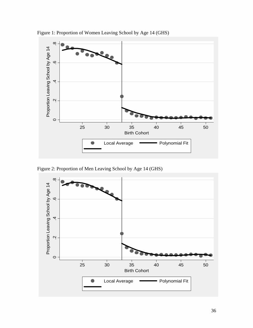
minimum age of 15. This reform had a very large impact on school leaving behaviour as
can be seen in Figures 1 and 2 – the fraction leaving school before age 15 fell from over
60% for the 1932 cohort to about 10% for the 1934 cohort. Oreopoulos (2006) and Clark
and Royer (2007) report similar impacts of the law change on schooling attainment.5
Assuming that other cohort level factors that impact adult wages did not also
systematically change for the 1933 cohort, we can identify schooling effects by
comparing adult wages of persons born just before 1933 to those born during or just after.
Empirical Specification
We estimate the relationships between the law change and our variables of
interest (schooling, wages and earnings) using a regression discontinuity approach (see
Imbens and Lemieux, 2008 and the references therein). The base specification regresses
the particular outcome on a quartic function of year of birth and a dummy variable for the
minimum school leaving age being 15.6 This global polynomial approach is a widely
used approach to regression discontinuity analysis (Lee and Card 2008) and has been
used to study the effects of the 1947 law change on mortality rates (Clark and Royer
2007). The quartic in cohort allows for smooth changes in outcomes over time and the
effect of the law change is identified from the discontinuity in the law variable when the
reform is implemented.7 Using the GHS, we present 2SLS estimates where the law
5 The fact that not everybody born after 1933 reports leaving school at age 15 or older can be ascribed to misreporting, individual non-compliance, and the fact that a few districts failed to provide sufficient school places for a while after the law was enacted. 6 To be consistent with Oreopoulos (2006) and to allow for random cohort-specific shocks, we report robust standard errors that allow for clustering by year of birth. An alternative would be to treat deviation from the polynomial fit as specification error and report standard robust standard errors (Chamberlain, 1994). 7 We use a quartic for consistency with Oreopoulos (2006). In practice, the estimates are very similar if a slightly lower or higher order polynomial is used. The visual impression from figures 3 – 8 is that the quartic function provides a good fit to the schooling and wage data. The results are also robust to varying

6
change is used as an instrumental variable for schooling. Because schooling is
unavailable in the NESPD, we take a two sample 2SLS approach to estimating the return
to schooling when using this dataset. This is described in Section 4.
3. Data
GHS
The General Household Survey (GHS) is a continuous national survey of people
living in private households, conducted on an annual basis by the Office for National
Statistics (ONS). The GHS started in 1971 and has been carried out continuously since
then, except for breaks in 1997-1998 when the survey was reviewed and 1999-2000 when
it was redeveloped. We use the 1979-1998 GHS surveys in our analysis.8 Being a
household survey, the GHS is subject to non-response and reporting error. The response
rates have varied over our sample period between a high of 85% in 1988 and a low of
72% in 1998.
The schooling variable we use is the age at which the person left school. This is
appropriate for our purposes as we are estimating the value of an extra year spent at
school (as distinct from the value of going to college or doing a PhD).9 We use usual
weekly earnings as our earnings measure and construct an hourly earnings variable in the
the cohorts studied or allowing the slope of the regression function to differ before versus after the law change. 8 We exclude the pre-1979 surveys from the analysis as earnings are measured very differently in this early period, referring to the year preceding the survey rather than to earnings in the week preceding the interview. We exclude post 1998 surveys as no survey was held in 1999 and the survey was relaunched in 2000 with a different design. Also, persons aged 28-64 in the 2000 and later surveys are born at least 3 years post-reform and so do not add much useful information to the regression discontinuity design. Oreopoulos (2006) used the 1984-1998 GHS surveys. 9 While there is also a measure of age when the person completed education, it is not as reliable as there appear to be many cases where people add some education after long absences from the system. Also, this variable is unavailable in the 1979-1982 GHS surveys and we need to use these years to have a large sample of pre-reform cohorts.
7
GHS using information on usual weekly earnings and usual weekly hours. We follow
Oreopoulos (2006) by including individuals who were born between 1921 and 1951 and
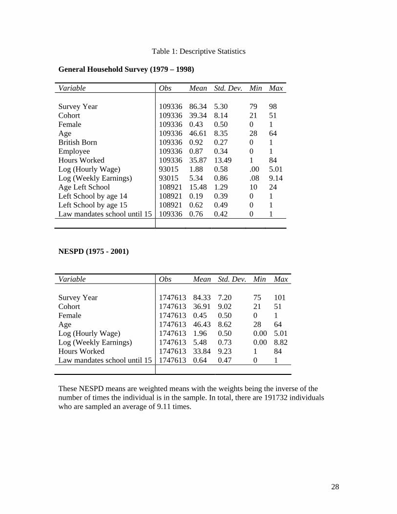
are aged between 28 and 64. Descriptive statistics for the sample are in Table 1 and
further details about the data construction are in the data appendix.
Because the cohorts impacted by the law are those born after April 1 1933,
approximately 3/4 of the 1933 cohort is impacted by the reform. In all analysis, we define
the law variable (LAW) as being equal to zero for persons born before 1933, 0.75 for
persons born in 1933, and one for persons born after 1933. While this coding increases
precision, IV estimates are very similar if we set LAW equal to 1 in 1933 or allow being
born in 1933 to have a different impact to being born in subsequent years or simply omit
the 1933 cohort altogether.
NESPD
The New Earnings Survey Panel Dataset (NESPD) is comprised of a random
sample of all individuals whose National Insurance numbers end in a given pair of digits.
Each year a questionnaire is directed to employers, who complete it on the basis of payroll
records for relevant employees. The questions relate to a specific week in April. Since the
same individuals are in the sample each year, the NESPD is a panel data set and our extract
runs from 1975 to 2001. Because National Insurance numbers are issued to all individuals
who reach the minimum school leaving age, the sampling frame of the survey is a random
sample of the labour force. Employers are legally required to complete the survey
questionnaire so the response rate is very high. Also, individuals can be tracked from
8
region to region and employer to employer through time using their National Insurance
numbers.10
Not everyone in the sample frame is captured every year as questionnaires are sent
to employers based on the employee’s current tax record. Individuals may not have a
current tax record if they have very recently changed jobs and the record has not been
updated, or if they do not earn enough to pay tax or National Insurance. However, given we
have a 26-year panel, we probably observe most working individuals at least once. In order
to give each person equal weight, we could randomly select one observation per individual
from the panel. Because this approach is wasteful with data, instead we use all observations
but weight each observation by the inverse of the number of times the person appears in the
panel. This gives each person equal weight irrespective of how frequently they appear in
the 26-year panel.11
Since the data are taken directly from the employer's payroll records, the earnings
and hours information in the NESPD are considered to be very accurate. The wage measure
we use is "gross weekly earnings excluding overtime divided by normal basic hours for
employees whose pay for the survey period was not affected by absence." We also
estimate weekly earnings specifications in which weekly earnings (including overtime)
replace hourly standard rates. Note that both full and part time workers are included in 10 Atkinson et al. (1981) and Atkinson et al. (1982) have compared the NESPD to a household survey, the Family Expenditure Survey, and found that the two surveys were fairly consistent in their hours and earnings patterns. 11 The NESPD under-samples individuals who earn less than the PAYE tax threshold in Britain and so are not subject to tax. The threshold has varied over time between £675 per year in 1975 and £4535 per year in 2001. To assess the extent of this problem, we have compared the proportion of observations in the NESPD sample that are under the threshold to the equivalent figure from the GHS sample. For men, there are fewer than 1% of these observations in either sample so it is not a relevant issue. For women, the proportions are 27% in the GHS and 18% in the NESPD (once we give each individual the same weight). We have tried reweighting the female regressions to get some sense as to what biases might arise. To do so, we gave a weight of 1.5 to observations in the NESPD that were below the tax threshold and a weight of 2/3 to observations that are above the threshold. This exercise had negligible effects on the estimates reported later in the paper. Thus, all indications suggest that this is not a big issue
9
estimation. Part-time workers constitute only about 2% of the male sample but make up
over 40% of the female sample. We have verified that omitting part time workers from
the sample does not change the estimates to any large extent. Descriptive statistics for the
sample are in Table 1 and further details about the data construction are in the data
appendix.
4. Pooled GHS Results and Comparison to Oreopoulos (2006)
As discussed above, the base first-stage specification regresses age left school on
a quartic function of cohort and the LAW variable. More formally, using the GHS, we
estimate the following equation:
iiii YOBfLAWSCH εαα +++= }{10 (1)
where i indexes individual, SCH is age left school, and }{ iYOBf is a quartic function of
year-of-birth. In some specifications, we add a quartic in age or a full set of age dummies.
When we pool men and women, we also include a gender dummy. We restrict the sample
to British-born persons aged between 28 and 64 who are members of the 1921 to 1951
cohorts.
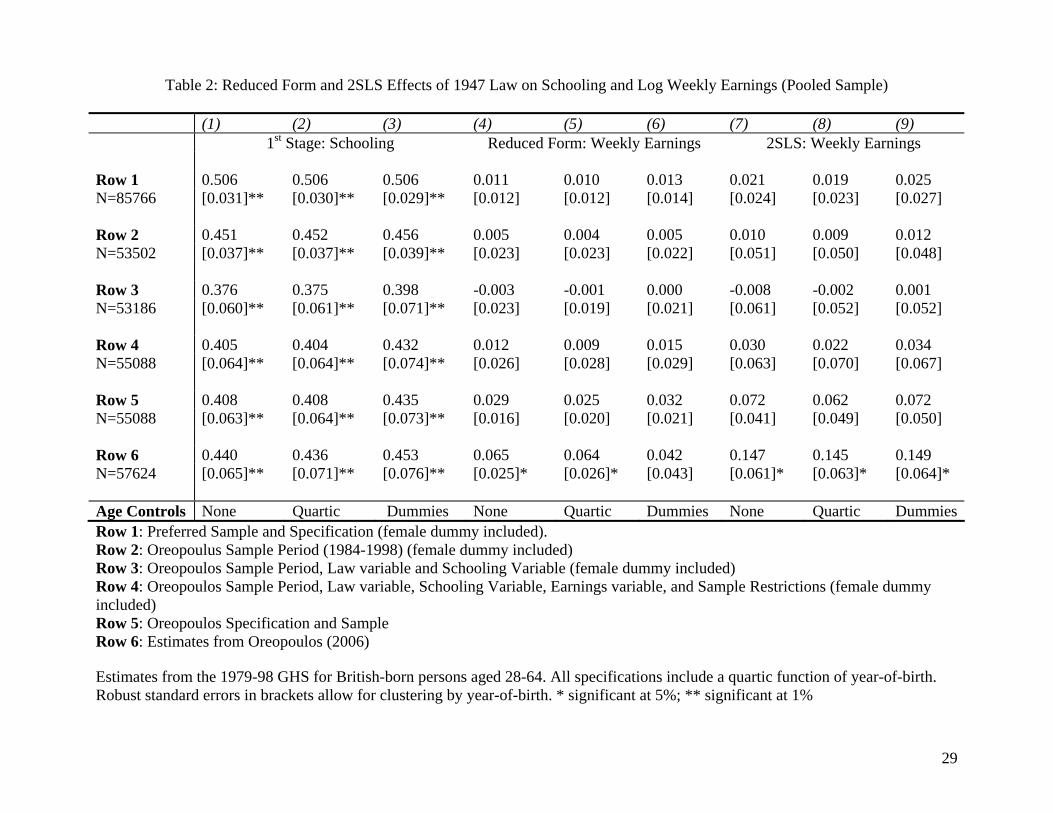
While there are good reasons to split the sample by gender, in Table 2 we follow
Oreopoulos (2006) in using a pooled sample of men and women. The first stage estimates
are presented in columns (1) to (3) of the first row of Table 2. The effect of the law is to
increase the average school leaving age by about a half of a year and the magnitude is
unaffected by the age specification chosen.
The reduced form specification regresses log weekly earnings on a quartic
function of cohort and the LAW variable. Specifically,
10
iiii eYOBgLAWY +++= }{ln 10 γγ (2)
where i indexes individual, Y is weekly earnings, and }{ iYOBg is a quartic function of
year-of-birth. Additional specifications add a quartic in age, and age dummies
respectively. Columns (4) to (6) of Row 1 of Table 2 report the reduced form effect of the
LAW variable on log weekly earnings. We find a statistically insignificant effect of the
law of about 1%.
Finally, in columns (7) to (9) of Row 1 of Table 2, we show the 2SLS estimates of
the effect of schooling on earnings. They imply that a year’s extra schooling increases
earnings by about 2% but the coefficients are always statistically insignificant. This is
obviously very different from the estimate of about 15% reported in Oreopoulos (2006) –
the estimates from his paper are listed in Row 6 of Table 2.12 However, our sample and
specification differs from his in many ways.
Oreopoulos Reconciliation
Oreopoulos kindly shared his programs with us and we used them to replicate his
sample restrictions and specification. In rows 2 to 5 of Table 2, we slowly move towards
his sample and specification. Firstly, like him, in Row 2 we exclude sample years 79-83.
The coefficient estimates don’t change much, but the standard errors increase by a lot.
The third row then switches from our schooling variable (age left school) to his (age left
education), and defines year of birth as in his programs (see the data appendix for
details). Additionally, as he does, we now define the LAW variable as being equal to 1
(rather than ¾) in 1933. The effect of these changes is to reduce the first stage effect of
12 Note that while Oreopoulos (2006) calls his dependent variable annual earnings, he constructs it by multiplying weekly earnings by 52. Therefore, in effect, the dependent variable in his regressions is weekly earnings.
11
the law from about .45 to .38 but the 2SLS point estimates are little changed. The fourth
row removes our hours restrictions and adds back in the earnings outliers we removed to
arrive at a sample defined in the same way as his.13 The point estimates rise a little but,
after all the adjustments, the 2SLS coefficient estimates are very similar to those from our
preferred sample and specification in Row 1 at about 2-3%. However, the 2SLS standard
errors are nearly 3 times larger in Row 4 than in Row 1.
When Oreopoulos (2006) pooled men and women, he did not include a gender
dummy. Therefore, in the 5th row of Table 2, we omit the gender dummy so that the
specification is exactly the same as his. This has the effect of increasing the 2SLS
estimates to about 6-7% but they are still not statistically significant.
Thus, after attempting to reconcile our sample and specifications, our estimate
using a pooled sample of men and women is 6-7% which is very different from the
Oreopoulos (2006) estimate of about 15%. Subsequent to releasing the working paper
version of this article (Devereux and Hart, 2008), we worked with Phil Oreopoulos to
understand this difference and discovered some problems in his STATA code. He cannot
replicate his 2006 findings and has now written a corrigendum (Oreopoulos 2008) with a
corrected table that has the same estimates as those in Row 5 of Table 2.14 We prefer the
estimates that include the female dummy so a reasonable conclusion from the GHS is an
average return to schooling of about 3%.
13 The hours and earnings restrictions we impose are detailed in the Data Appendix. 14 The first stage and reduced form coefficients in Oreopoulos (2008) are identical to those in Row 5 in Table 2. There are some small differences in the 2SLS coefficients at the 3rd decimal point and we do not understand their source. We have verified, however, that our 2SLS coefficients equal the reduced form coefficient divided by the first stage coefficient (as they should).

12
5. GHS and NESPD Estimates by Gender
Labour market experiences were very different for men and women in these
cohorts so, in the rest of the analysis, we split the sample by sex. We report estimates
using both the GHS and the NESPD in Tables 3 and 4. We use exactly the same sample
restrictions and specification with the NESPD as we did with the GHS. However, one
point to note is that the NESPD includes immigrants and excludes self-employed
persons.15
1st Stage Estimates
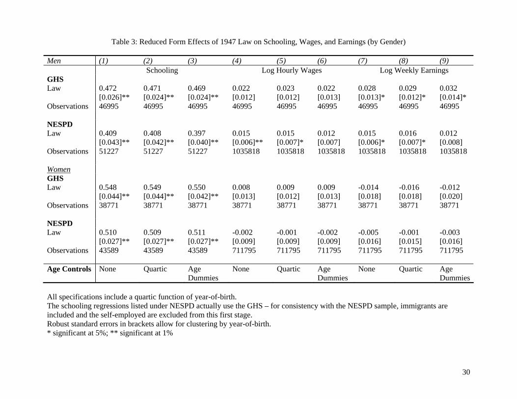
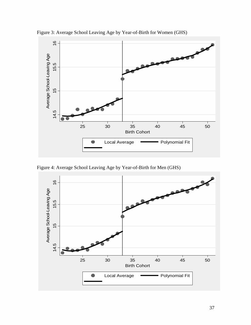
The first stage estimates by gender are in the first and third panels of Table 3. The
effect of the law is to increase the average school leaving age by about .47 of a year for
men and .55 of a year for women and these are both strongly statistically significant.
While not reported in the table, the law reduced the proportion who finished school at 14
or younger by .47 (.02) for men and .49 (.02) for women.16 Figures 1 to 4 display the
estimates graphically by plotting by year of birth. The polynomial fits in these figures are
created using the baseline specification of a quartic in cohort. The break in 1933 is very
clear.
We also use the GHS to estimate a separate 1st stage regression to use with the
NESPD earnings data. For comparability with the NESPD sample, we restrict this GHS
sample in the first-stage to employed persons aged between 28 and 64 who are members
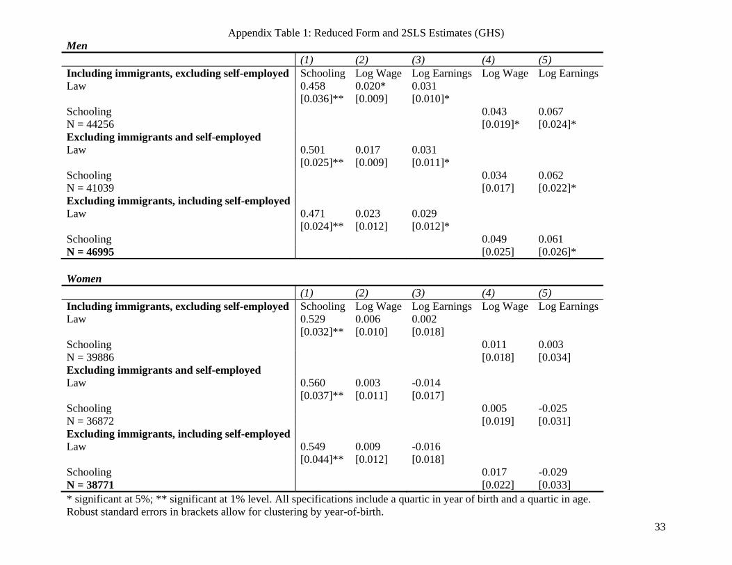
of the 1921 to 1951 cohorts and work between 1 and 84 hours a week. Also, for 15 As can be seen in Appendix Table 1, the GHS estimates are not very sensitive to the inclusion or exclusion of immigrants or the self-employed. For this reason, we don’t believe that our NESPD estimates are seriously impacted by the inclusion of immigrants and exclusion of self-employed. As can be seen in Table 1, only about 8% of our GHS sample are immigrants and 12% are self-employed. We have calculated similar percentages for these cohorts using the British Labour Force Survey. 16 The effects of the law are strongly concentrated at age 14 – 15. The effect of the law on probability finish by age 15 is -.02 (.01) for men and -.05 (.02) for women. The equivalent figures for age 16 are small -- .02 (.01) for men and .01 (.01) for women.

13
consistency with the NESPD sample exclusions, we exclude the self-employed and
include immigrants (even though the GHS has country of birth indicators).
These first stage estimates are presented in the second and fourth panels of Table
3 (under the NESPD heading). The effect of the law is to increase the average school
leaving age by about .4 of a year for men and .5 of a year for women and these are both
strongly statistically significant. These effects are a little smaller than in the earlier GHS
sample and the difference is primarily due to the presence of immigrants in this NESPD-
compatible sample.
Reduced Form Effects on Hourly Wages and Weekly Earnings
The reduced form estimates for hourly wages and weekly earnings from the GHS
and NESPD are in columns (4) to (9) of Table 3. The results differ between men and
women. For men, the reduced form estimate in the NESPD of the effect of the law
change on both log wages and log earnings is about .015 (.007) so the law increases
wages by about 1.5%. In the GHS, the estimates for men are a little larger at about 2%
for wages and 3% for earnings. For women, the estimate is always about zero in both
datasets with a standard error of .01 for wages and .02 for earnings.17
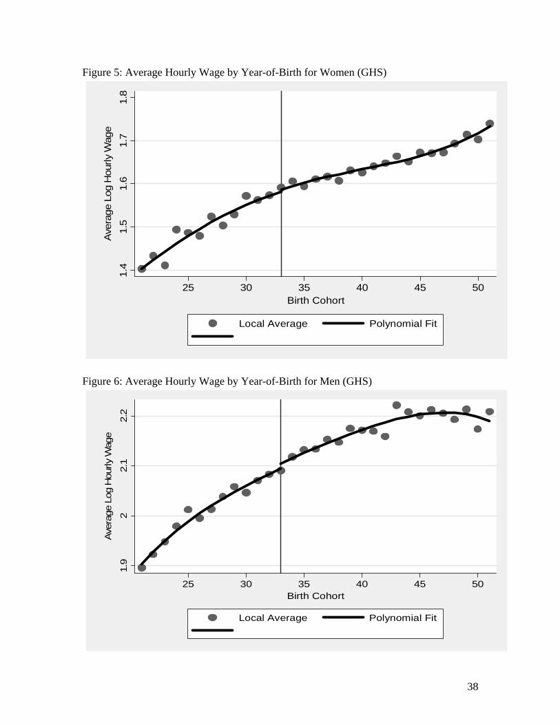
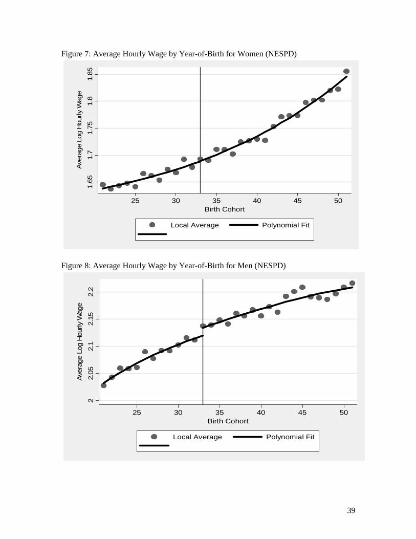
Figures 5-8 display the hourly wage estimates graphically. For men, there is a
clear break in the series in 1933. For women, it is equally clear that there is no break in
the series in 1933.
17 The reduced form effects are almost identical when we use median regression rather than mean regression. For example, in the NESPD for the specification with a quartic in age, reduced form effects for men are .016 (.006) and .017 (.005) for wages and earnings respectively; for women the equivalent numbers are -.003 (.006) and .008 (.012)). This indicates that our estimates are not being strongly impacted by outliers.
14
Instrumental Variables Estimates
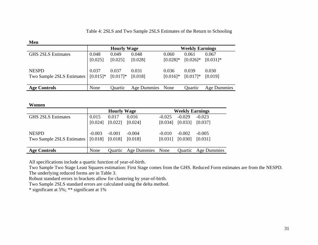
The IV estimates for both datasets are in Table 4. In the GHS, the 2SLS estimates
for men are a marginally significant effect of about 5% for wages and a statistically
significant effect of about 6% for weekly earnings. We cannot reject zero effects of
schooling on wages or earnings of women and the point estimates are always very close
to zero.18
Given that the first stage and reduced form regressions come from different
datasets, it is not possible to do conventional 2SLS to estimate the return to an extra year
in school when we use NESPD wage and earnings data. Instead we use Two Sample Two
Stage Least Squares (TS2SLS) (Angrist and Krueger 1992; Inoue and Solon 2006). This
is implemented by forming the predicted value of schooling using the first stage
coefficients estimated in the GHS and the actual explanatory variables from the NESPD.
We then use the NESPD to regress the log wage on the predicted value of schooling and
the usual explanatory variables.
Note that because we have one instrument and our specification is just identified,
the TS2SLS estimator is simply the reduced form effect of the law divided by the first
stage effect.19 That is, using the estimates from equations (1) and (2), the estimated return
to schooling is 111 ˆ/ˆˆ αγβ = .
18 We observe wages only for individuals who work and the law may systematically impact employment probabilities. Interestingly, we find that there is a small but statistically significant negative effect of the law on employment in the GHS for both men and women. This is not just an early retirement effect as it is also present when the sample is restricted to persons aged 60 or less. Assuming that the non-employed would tend to have lower wages if they worked, this suggests that our estimates may, if anything, be biased upwards due to this type of selection. 19 In calculating the TS2SLS standard errors, we use the delta method to allow for the fact that the predicted value of schooling contains sampling error.
15
The TS2SLS estimates are in the second and fourth panels of Table 4. As
suggested by the reduced forms, the return to schooling is essentially zero for women but
positive for men. The size of the effect for men is about .04, implying that an extra year
of schooling increases wages and earnings by about 4%. This is a little smaller than the
corresponding estimates from the GHS but the differences are really quite small.
Many low skilled people quit working before age 65 in Britain – Banks and
Blundell (2005) show that, in the 1980-2000 period, the employment rate of men aged
60-64 is only about 40%. Our estimates are very similar when we omit persons aged over
60. This can be seen in Appendix Tables 2 and 3 where we show results analogous to
those in tables 2 and 4.
6. Estimates using Northern Ireland as a Control Group
Oreopoulos (2006) also reports regressions that pool data from the GHS and the
Northern Ireland Continuous Household Survey (CHS).20 In these specifications he
controls for a quartic in cohort (sometimes also age controls) and a Northern Ireland (NI)
dummy, exploiting the fact that the school leaving age was raised later in NI than in the
rest of the UK. The instrument is a dummy variable for whether the minimum school
leaving age is 15 – this changes from zero to one for the 1933 cohort in Britain but does
not change from zero to one until the 1943 cohort in NI. As before, the cohorts included
are those born between 1921 and 1951. This approach assumes that cohort effects and age
effects are the same in Britain and NI and this may be a strong assumption given that
Northern Ireland is a unique place with its issues of religious discrimination that
20 The CHS surveys he uses are those from 1986-91, as well as 1996, 1998, and 1999. Earnings are reported in intervals in the CHS and he uses the midpoint of each interval in estimation.
16
generally do not apply to the rest of the UK.21 While attitudes to identifying assumptions
are necessarily subjective, we do not find this approach as compelling as the RD design
using British data alone.22 However, we will provide a brief analysis.
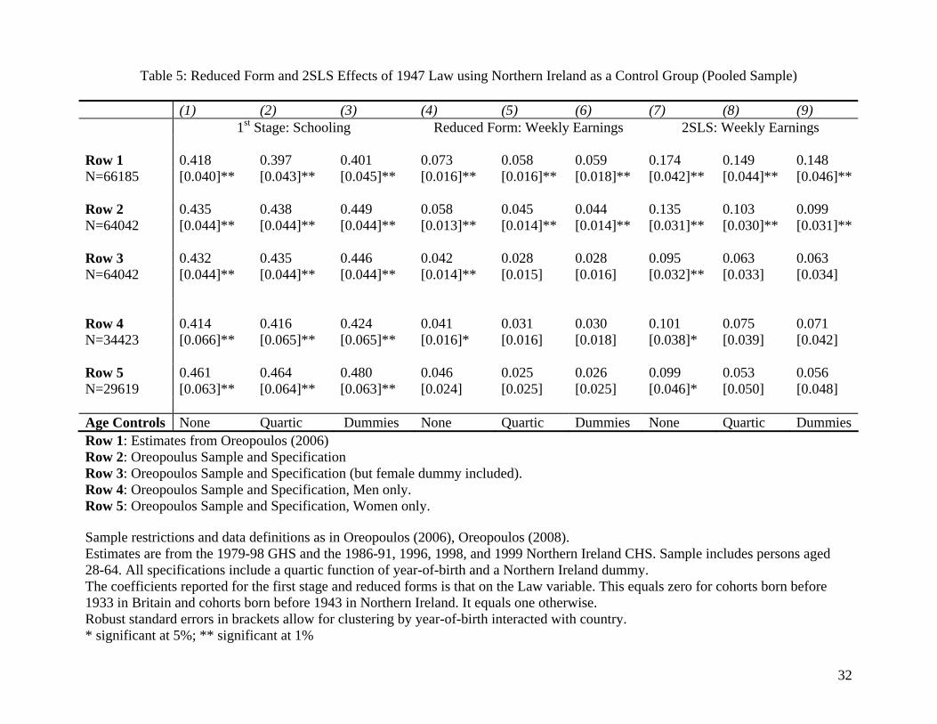
In Table 5, we start in Row 1 by listing the estimates from Oreopoulos (2006). In
the specifications with age controls, he found 2SLS estimates of about 15%. However,
these estimates are not replicable. Therefore, in Row 2, we report estimates that utilise the
sample and variable definitions used in his corrigendum (Oreopoulos 2008). Now the
estimates with age controls imply a lower return to schooling of about 10%. In Row 3, we
add a dummy for gender to the specification and this further reduces the pooled 2SLS
estimate to about 6% and it is no longer statistically significant. Thus the pooled Britain-
NI sample provides estimates that are not so different from the RD approach that just uses
British data.
In the final two rows of Table 5, we split the sample by sex. When age controls
are included the 2SLS estimate for men is about 7% and that for women is about 5%.
Neither is statistically significant and, given the standard errors, neither can be considered
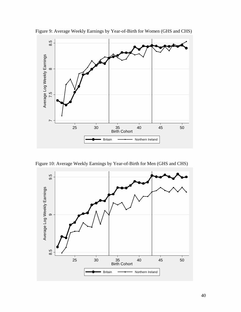
very different to what we found earlier using the RD approach.23 Figures 9 and 10 show
average log earnings by cohort for women and men in Britain and NI and it is clear that
there is a lot of cohort-level variation that cannot reasonably be explained by either the
British or NI law change. These pictures strengthen our view that the RD approach using
British data alone is a more compelling one.
21 Also, Figure 9 in his paper shows that cohort-level changes in earnings appear to often diverge between Britain and Northern Ireland, even in years when there are no changes in compulsory schooling laws, potentially invalidating the assumption that cohort effects are the same in both regions. 22 It is clear from his paper that Oreopoulos (2006) also considers the RD approach to be particularly compelling. 23 The CHS data are not sufficiently rich to allow us to use variable definitions and sample restrictions that are consistent with our preferred GHS ones so we have not attempted to do so.
17
7. Discussion
We have found 2SLS returns to schooling of about 4-7% for men and zero for
women. A natural comparison point is to OLS estimates from the GHS. We find very
high OLS returns using age left school but these estimates are a bit problematic as, for
example, the difference between finishing at 16 versus 18 may be more than 2 years of
education as many of those completing school at 18 go on to further study. Therefore, we
report OLS estimates using age left education as our schooling variable.24 For hourly
wages, the coefficient on age left education is .07 (.002) for men and .06 (.001) for
women. For weekly earnings, the analogous coefficients are .07 (.001) and .12 (.002) for
men and women respectively. These suggest that either the value of an additional year in
school is quite high for these cohorts or there is a lot of selection in terms of who leaves
school early. Our analysis using the change in the compulsory schooling law suggests the
latter explanation is particularly important for women.
There are many studies that report estimates of the return to schooling using
compulsory schooling laws. For example, Angrist and Krueger (1991) and Oreopoulos
(2006) for the U.S., Black et al. (2005) for Norway, Grenet (2009) for France and Britain,
and Pischke and von Wachter (2008) for Germany. The U.S. IV estimates are similar or
higher than OLS but the estimates from the three papers using European data are all
lower than OLS and sometimes very low – Pischke and von Wachter report estimates
24 This involves restricting the sample to the 1983 survey and after as age left education is unavailable before then. Also, since there are reported ages as high as 35, we censor age left education at 23 for the purposes of the OLS estimation.

18
suggesting zero returns to schooling in Germany.25 Our estimates are, thus, generally
consistent with other European findings.
Why have we found the returns to compulsory schooling to be low? Grenet (2009)
suggests that a key element in determining the return to compulsory schooling is the
extent to which more restrictive laws result in increased qualifications. Because the 1947
reform only induced participation until age 15, it would not have been expected to
increase the proportion of people who held qualifications such as O-levels. We have
tested this empirically and found no evidence of any effect of the law change on the
probability of holding an academic credential. Grenet (2009) finds somewhat larger
estimates of the return to schooling using the 1973 British increase in the compulsory
schooling age from 15 to 16 that did lead to a higher proportion of people obtaining some
academic credential.
Another possibility relates to heterogeneous returns to schooling. Imbens and
Angrist (1994) show that, under a monotonicity assumption, the IV estimator provides a
Local Average Treatment Effect (LATE). In other words, it calculates the average effect
of the treatment for compliers (individuals whose behaviour is changed by the
instrument) only. In our case, the monotonicity assumption implies that the increase in
the compulsory schooling age from 14 to 15 does not cause anyone who would have
stayed until aged 15+ to now leave at age 14. The IV estimate provides no information
about the returns to schooling for always-takers (people who would have stayed in school
until at least age 15 irrespective of the legal rule) or never-takers (people who drop out
25 On the other hand, the Swedish study of Meghir and Palme (2005) implies an average return to compulsory schooling of about 8%. Note that, in both Norway and Sweden, the reforms involved other elements in addition to raising the compulsory schooling age and so quality of schooling may have also changed.
19
before age 15 irrespective of the legal rule). In our case, both of these groups exist as
almost 40% stayed until 15+ before the law change, and about 10% dropped out before
age 15 after the law change. This means that, without extrapolation, the LATE is
uninformative about the ATE. However, as pointed out by Oreopoulos (2006), it is
reasonable to suppose that as the number of compliers becomes an increasingly large
proportion of the sample, the LATE should converge towards the ATE.
Thus, one possibility is that the estimates for Britain (where the 1947 reform
affected about half the relevant population) suggest the ATE is much smaller than the
LATE. By this logic, the much larger returns found in the U.S. may have been found
because returns are highest for marginal individuals and a very small proportion are
affected by the U.S. law changes. Interestingly, Pischke and von Wachter (2008) find
zero estimates for Germany where a similarly large proportion were impacted by the
compulsory schooling law change they study. On the other hand, Grenet (2009) finds
zero returns for France and Black et al. (2005) report small returns for Norway in
situations where a much smaller proportion of the underlying population changed
behaviour as a result of law changes.
8. Conclusions
The 1947 change in the British compulsory schooling law has enabled us to
estimate the returns to extra schooling for men and women in a situation where about half
the population leave school at the earliest possible age. We find no evidence of any wage
or earnings return for women and our preferred estimates suggest a modest return to an
extra year of schooling of 4 to 7% for men. The estimates are similar in both the NESPD

20
and GHS and are generally consistent with other studies of compulsory schooling laws
using European data.
Our estimates also may help explain the puzzle of why half the British population
dropped out of school as early as they could given the returns to schooling are apparently
so high. One simple explanation is that the returns to additional schooling were actually
quite low for this group and it was rational to leave school early. While it is difficult to
quantify the costs of an extra year of schooling, this story is certainly consistent with our
results for women in this paper.

21
Data Appendix
2001 New Earnings Survey Panel Data-set (NESPD)
This dataset contains information from 1975 to 2001. We include part-time and full-time
earners aged 18 to 64 as on January 1st of the survey year. We exclude cases where
earnings are affected by absence. We also exclude observations if their “Hourly Earnings
excluding overtime” is missing or if their normal basic hours are missing. Because age is
as at January 1st, year of birth is constructed as being equal to survey year – age -1 and
we keep the 1921-51 cohorts. We deflate wages and earnings using the British Retail Price
Index and drop cases for which hourly wage observations are less than £1 or more than
£150 (in December 2001 pounds). These exclusions are similar to those used by Card
(1999). They imply the exclusion of 136 male observations (682 female) that have wages
less than £1 and 91 male observations (0 female) that have wages greater than £150. To
put these numbers in context, the minimum wage was £3.70 in 2001. We exclude the
small number of cases where weekly hours are greater than 84 (99 cases), less than 1, or
missing.
General Household Survey (GHS)
We use GHS files from 1979 to 1998 (there is no 1997 survey) and include persons who
report their age as being between 28 and 64.
Year of Birth: Year of birth is reported in the data from 1986-95 and in 1998. Year of
birth is also available for women aged 16-49 in the 1983-1985 surveys and we use this
information where available. For cases where year of birth is unavailable, we impute year

22
of birth as being (survey year – age) for persons who are interviewed between July and
December, and as being (survey year – age – 1) for persons interviewed between January
and June.
Earnings Measures: The usual weekly earnings measures in the GHS change in exact
definition and name over time. We use PAYWEEK for the 1979-82 surveys, UGE for the
1984-91 surveys, GEIND for the 1992-1996 surveys, and GREARN for the 1998 survey.
Unlike the other weekly earnings measures, PAYWEEK excludes self-employment
income so we add any positive self-employment income using the INCSELF variable.
UGE is missing in the 1983 survey so we construct it in the same way that UGE is
constructed by the GHS data team for the 1984 survey year. We construct an hourly
earnings variable in the GHS using information on usual weekly earnings and usual
weekly hours (WORKHRS). One drawback is that the earnings information includes
overtime earnings but the hours variable excludes overtime hours. Despite this problem,
we report estimates using the hourly wage variable in addition to weekly earnings.
Manning (2000) also uses this variable and shows that it is highly correlated with the true
hourly wage (correlation=.98) because average overtime hours are relatively short (less
than 3 per week) and because overtime hours are very weakly correlated with hourly
earnings. As in the NESPD, we deflate wages and earnings using the British Retail Price
Index. We set to missing cases for which hourly wage observations are less than £1 or more
than £150 (in December 2001 pounds). We exclude cases where weekly hours are greater
than 84, less than 1, or missing.
Schooling: Our measure of schooling is age left school. The relevant variables are
AGELFTS from 1979-82 and AGELFTSC from 1983-98. We set schooling to missing
23
for cases in which age left school is reported to be less than 10, greater than 24, or greater
than the respondent’s reported age.
Data for specifications in rows 3-5 of Table 2 and in Table 5
Variable construction and sample restrictions for these estimates are taken from
Oreopoulos (2006) and from his STATA programs (with his kind assistance). All GHS
variables are constructed from 1984-1998 as this is the time period he used in estimation.
Full details can be found in Oreopoulos (2006), Oreopoulos (2008), and in his STATA
programs on the AER website.
GHS: He uses Terminal Age of Education (TEA) as his schooling measure. For weekly
earnings, he uses UGE for the 1984-91 surveys, GEIND for the 1992-1996 surveys, and
GREARN for the 1998 survey. He multiplies weekly earnings by 52 and refers to it as
annual earnings. For year of birth, he uses that reported in the data in survey years 1987-
95. He imputes year of birth as equal to survey year – age in other years. He drops cases
with nominal earnings of 10,000 per week or more. His regressions always use nominal
rather than real earnings.
Northern Ireland Data: The Continuous Household Survey (CHS) data from Northern
Ireland used in Table 5 are exactly as defined by Oreopoulos (2006) and Oreopoulos
(2008). The CHS surveys used are those from 1986-91, as well as 1996, 1998, and 1999.
Earnings are reported in intervals in the CHS and the midpoint of each interval is used in
estimation.

24
References
Angrist, Joshua D. and Alan B. Krueger (1991). “Does Compulsory Schooling
Attendance Affect Schooling and Earnings?,” Quarterly Journal of Economics,
106, 979-1014.
Angrist, Joshua D. and Alan B. Krueger (1992). “The Effect of Age at School Entry on
Educational Attainment: An Application of Instrumental Variables with Moments
from Two Samples,” Journal of the American Statistical Association, 87, 328-36.
Atkinson, A.B., Micklewright, J., Stern, N.H. (1981). “A comparison of the FES and
NES 1971–1977: Part I. Characteristics of the sample.” Social Science Research
Council Programme on Taxation, Incentives and the Distribution of Income
Working Paper No. 27.
Atkinson, A.B., Micklewright, J., Stern, N.H. (1982). “A comparison of the FES and
NES 1971–1977: Part II. Hours and earnings.” Social Science Research Council
Programme on Taxation, Incentives and the Distribution of Income Working
Paper No. 32.
Banks James and Richard Blundell (2005). “Private Pension Arrangements and
Retirement in Britain,” Fiscal Studies 26(1), 35-53.
Black, Sandra E., Paul J. Devereux, and Kjell G. Salvanes. (2005). “Why the Apple
Doesn’t Fall Far: Understanding Intergenerational Transmission of Human
Capital,” American Economic Review, 95(1), 437-449.
Black, Sandra E., Paul J. Devereux, and Kjell G. Salvanes. (2008). “Staying in the
Classroom and out of the Maternity Ward? The Effect of Compulsory Schooling
Laws on Teenage Births,” Economic Journal, 118(530), 1025-54.
25
Card, David (1999). “The Causal Effect of Education on Earnings,” in Orley Ashenfelter
and David Card (eds.), Handbook of Labor Economics, Volume 3A, North-
Holland.
Chamberlain, Gary (1994). “Quantile Regression, Censoring, and the Structure of
Wages,” in C. A. Sims, ed., Advances in Econometrics, Sixth World Congress,
Vol. 1, Cambridge: Cambridge University Press.
Clark, Damon and Heather Royer (2007). “The Effect of Education on Adult Mortality
and Health: Evidence from the United Kingdom,” mimeo, July.
Devereux, Paul J. and Robert A. Hart (2008). “Forced to be Rich? Returns to Compulsory
Schooling in Britain”, IZA Discussion Paper #3305, January.
Galindo-Rueda, Fernando (2003). “The Intergenerational Effect of Parental Schooling:
Evidence from the British 1947 School Leaving Age Reform,” mimeo.
Grenet, Julien (2009) “Is it Enough to Increase Compulsory Education to Raise Earnings?
Evidence from French and British Compulsory Schooling Laws”, CEP working
paper, April.
Harmon Colm and Ian Walker. (1995), “Estimates of the Economic Return to Schooling
for the United Kingdom,” American Economic Review 85, 1278-1296.
Imbens, Guido and Joshua Angrist. (1994). “Identification and Estimation of Local
Average Treatment Effects,” Econometrica, 62(2), 467-476.
Imbens, Guido and Thomas Lemieux. (2008). “Regression Discontinuity Designs: A
Guide to Practice,” Journal of Econometrics, 142(2), 615-35.
Inoue, Atsushi, and Gary Solon. (2006). “Two-Sample Instrumental Variables
Estimators,” Working Paper.
26
Lee, David, and David Card (2008). “Regression Discontinuity Inference with
Specification Error,” Journal of Econometrics, 142(2), 655-74.
Lindeboom Maarten, Ana Llena Nozal, and Bas van der Klaauw (2009), “Parental
Education and Child Health: Evidence from a Schooling Reform,” Journal of
Health Economics 28(1) January, 109-131.
Lleras-Muney, Adriana. (2005), “The Relationship Between Education and Adult
Mortality in the United States,” Review of Economic Studies 72, 189-221.
Manning, Alan (2000), “Movin’ on Up: Interpreting the Earnings-Experience Profile,”
Bulletin of Economic Research 52(4), 261-295.
Meghir, Costas and Marten Palme (2005) “Educational Reform, Ability and Parental
Background,” American Economic Review, Vol. 95, No. 1 (March), 414-424.
Milligan Kevin, Moretti Enrico, Oreopoulos Philip. (2004) “Does education improve
citizenship? Evidence from the United States and the United Kingdom,” Journal
of Public Economics, 88:1667–95.
Moretti, Enrico and Lance Lochner. (2004), “The Effect of Education on Criminal
Activity: Evidence from Prison Inmates, Arrests and Self-Reports,” American
Economic Review 94(1).
Oreopoulos, Philip (2006), “Estimating Average and Local Average Treatment Effects of
Education When Compulsory Schooling Laws Really Matter, American Economic
Review 96, 152-175.
Oreopoulos, Philip (2008), “Estimating Average and Local Average Treatment Effects of
Education When Compulsory Schooling Laws Really Matter: Corrigendum”, August.
27
Oreopoulos Philip, Marianne E. Page, and Ann Huff Stevens (2006), “The
Intergenerational Effects of Compulsory Schooling,” Journal of Labor Economics
24(4), 729-760.
Pischke, Jorn-Steffen and Till von Wachter (2008), “Zero Returns to Compulsory
Schooling in Germany: Evidence and Interpretation, Review of Economics and
Statistics 90(3) August, 592-598.
28
Table 1: Descriptive Statistics
General Household Survey (1979 – 1998)
Variable Obs Mean Std. Dev. Min Max Survey Year 109336 86.34 5.30 79 98 Cohort 109336 39.34 8.14 21 51 Female 109336 0.43 0.50 0 1 Age 109336 46.61 8.35 28 64 British Born 109336 0.92 0.27 0 1 Employee 109336 0.87 0.34 0 1 Hours Worked 109336 35.87 13.49 1 84 Log (Hourly Wage) 93015 1.88 0.58 .00 5.01 Log (Weekly Earnings) 93015 5.34 0.86 .08 9.14 Age Left School 108921 15.48 1.29 10 24 Left School by age 14 108921 0.19 0.39 0 1 Left School by age 15 108921 0.62 0.49 0 1 Law mandates school until 15 109336 0.76 0.42 0 1 NESPD (1975 - 2001)
Variable Obs Mean Std. Dev. Min Max Survey Year 1747613 84.33 7.20 75 101 Cohort 1747613 36.91 9.02 21 51 Female 1747613 0.45 0.50 0 1 Age 1747613 46.43 8.62 28 64 Log (Hourly Wage) 1747613 1.96 0.50 0.00 5.01 Log (Weekly Earnings) 1747613 5.48 0.73 0.00 8.82 Hours Worked 1747613 33.84 9.23 1 84 Law mandates school until 15 1747613 0.64 0.47 0 1 These NESPD means are weighted means with the weights being the inverse of the number of times the individual is in the sample. In total, there are 191732 individuals who are sampled an average of 9.11 times.
29
Table 2: Reduced Form and 2SLS Effects of 1947 Law on Schooling and Log Weekly Earnings (Pooled Sample) (1) (2) (3) (4) (5) (6) (7) (8) (9)
1st Stage: Schooling Reduced Form: Weekly Earnings 2SLS: Weekly Earnings Row 1 0.506 0.506 0.506 0.011 0.010 0.013 0.021 0.019 0.025 N=85766 [0.031]** [0.030]** [0.029]** [0.012] [0.012] [0.014] [0.024] [0.023] [0.027] Row 2 0.451 0.452 0.456 0.005 0.004 0.005 0.010 0.009 0.012 N=53502 [0.037]** [0.037]** [0.039]** [0.023] [0.023] [0.022] [0.051] [0.050] [0.048] Row 3 0.376 0.375 0.398 -0.003 -0.001 0.000 -0.008 -0.002 0.001 N=53186 [0.060]** [0.061]** [0.071]** [0.023] [0.019] [0.021] [0.061] [0.052] [0.052] Row 4 0.405 0.404 0.432 0.012 0.009 0.015 0.030 0.022 0.034 N=55088 [0.064]** [0.064]** [0.074]** [0.026] [0.028] [0.029] [0.063] [0.070] [0.067] Row 5 0.408 0.408 0.435 0.029 0.025 0.032 0.072 0.062 0.072 N=55088 [0.063]** [0.064]** [0.073]** [0.016] [0.020] [0.021] [0.041] [0.049] [0.050] Row 6 0.440 0.436 0.453 0.065 0.064 0.042 0.147 0.145 0.149 N=57624 [0.065]** [0.071]** [0.076]** [0.025]* [0.026]* [0.043] [0.061]* [0.063]* [0.064]* Age Controls None Quartic Dummies None Quartic Dummies None Quartic DummiesRow 1: Preferred Sample and Specification (female dummy included). Row 2: Oreopoulus Sample Period (1984-1998) (female dummy included) Row 3: Oreopoulos Sample Period, Law variable and Schooling Variable (female dummy included) Row 4: Oreopoulos Sample Period, Law variable, Schooling Variable, Earnings variable, and Sample Restrictions (female dummy included) Row 5: Oreopoulos Specification and Sample Row 6: Estimates from Oreopoulos (2006) Estimates from the 1979-98 GHS for British-born persons aged 28-64. All specifications include a quartic function of year-of-birth. Robust standard errors in brackets allow for clustering by year-of-birth. * significant at 5%; ** significant at 1%
30
Table 3: Reduced Form Effects of 1947 Law on Schooling, Wages, and Earnings (by Gender) Men (1) (2) (3) (4) (5) (6) (7) (8) (9)
Schooling Log Hourly Wages Log Weekly Earnings GHS Law 0.472 0.471 0.469 0.022 0.023 0.022 0.028 0.029 0.032 [0.026]** [0.024]** [0.024]** [0.012] [0.012] [0.013] [0.013]* [0.012]* [0.014]* Observations 46995 46995 46995 46995 46995 46995 46995 46995 46995 NESPD Law 0.409 0.408 0.397 0.015 0.015 0.012 0.015 0.016 0.012 [0.043]** [0.042]** [0.040]** [0.006]** [0.007]* [0.007] [0.006]* [0.007]* [0.008] Observations 51227 51227 51227 1035818 1035818 1035818 1035818 1035818 1035818 Women GHS Law 0.548 0.549 0.550 0.008 0.009 0.009 -0.014 -0.016 -0.012 [0.044]** [0.044]** [0.042]** [0.013] [0.012] [0.013] [0.018] [0.018] [0.020] Observations 38771 38771 38771 38771 38771 38771 38771 38771 38771 NESPD Law 0.510 0.509 0.511 -0.002 -0.001 -0.002 -0.005 -0.001 -0.003 [0.027]** [0.027]** [0.027]** [0.009] [0.009] [0.009] [0.016] [0.015] [0.016] Observations 43589 43589 43589 711795 711795 711795 711795 711795 711795 Age Controls None Quartic Age
Dummies None Quartic Age
Dummies None Quartic Age
Dummies All specifications include a quartic function of year-of-birth. The schooling regressions listed under NESPD actually use the GHS – for consistency with the NESPD sample, immigrants are included and the self-employed are excluded from this first stage. Robust standard errors in brackets allow for clustering by year-of-birth. * significant at 5%; ** significant at 1%
31
Table 4: 2SLS and Two Sample 2SLS Estimates of the Return to Schooling
Men Hourly Wage Weekly Earnings GHS 2SLS Estimates 0.048 0.049 0.048 0.060 0.061 0.067 [0.025] [0.025] [0.028] [0.028]* [0.026]* [0.031]* NESPD 0.037 0.037 0.031 0.036 0.039 0.030 Two Sample 2SLS Estimates [0.015]* [0.017]* [0.018] [0.016]* [0.017]* [0.019] Age Controls None Quartic Age Dummies None Quartic Age Dummies Women Hourly Wage Weekly Earnings GHS 2SLS Estimates 0.015 0.017 0.016 -0.025 -0.029 -0.023 [0.024] [0.022] [0.024] [0.034] [0.033] [0.037] NESPD -0.003 -0.001 -0.004 -0.010 -0.002 -0.005 Two Sample 2SLS Estimates [0.018] [0.018] [0.018] [0.031] [0.030] [0.031] Age Controls None Quartic Age Dummies None Quartic Age Dummies All specifications include a quartic function of year-of-birth. Two Sample Two Stage Least Squares estimation: First Stage comes from the GHS. Reduced Form estimates are from the NESPD. The underlying reduced forms are in Table 3. Robust standard errors in brackets allow for clustering by year-of-birth. Two Sample 2SLS standard errors are calculated using the delta method. * significant at 5%; ** significant at 1%
32
Table 5: Reduced Form and 2SLS Effects of 1947 Law using Northern Ireland as a Control Group (Pooled Sample) (1) (2) (3) (4) (5) (6) (7) (8) (9)
1st Stage: Schooling Reduced Form: Weekly Earnings 2SLS: Weekly Earnings Row 1 0.418 0.397 0.401 0.073 0.058 0.059 0.174 0.149 0.148 N=66185 [0.040]** [0.043]** [0.045]** [0.016]** [0.016]** [0.018]** [0.042]** [0.044]** [0.046]** Row 2 0.435 0.438 0.449 0.058 0.045 0.044 0.135 0.103 0.099 N=64042 [0.044]** [0.044]** [0.044]** [0.013]** [0.014]** [0.014]** [0.031]** [0.030]** [0.031]** Row 3 0.432 0.435 0.446 0.042 0.028 0.028 0.095 0.063 0.063 N=64042 [0.044]** [0.044]** [0.044]** [0.014]** [0.015] [0.016] [0.032]** [0.033] [0.034] Row 4 0.414 0.416 0.424 0.041 0.031 0.030 0.101 0.075 0.071 N=34423 [0.066]** [0.065]** [0.065]** [0.016]* [0.016] [0.018] [0.038]* [0.039] [0.042] Row 5 0.461 0.464 0.480 0.046 0.025 0.026 0.099 0.053 0.056 N=29619 [0.063]** [0.064]** [0.063]** [0.024] [0.025] [0.025] [0.046]* [0.050] [0.048] Age Controls None Quartic Dummies None Quartic Dummies None Quartic DummiesRow 1: Estimates from Oreopoulos (2006) Row 2: Oreopoulus Sample and Specification Row 3: Oreopoulos Sample and Specification (but female dummy included). Row 4: Oreopoulos Sample and Specification, Men only. Row 5: Oreopoulos Sample and Specification, Women only. Sample restrictions and data definitions as in Oreopoulos (2006), Oreopoulos (2008). Estimates are from the 1979-98 GHS and the 1986-91, 1996, 1998, and 1999 Northern Ireland CHS. Sample includes persons aged 28-64. All specifications include a quartic function of year-of-birth and a Northern Ireland dummy. The coefficients reported for the first stage and reduced forms is that on the Law variable. This equals zero for cohorts born before 1933 in Britain and cohorts born before 1943 in Northern Ireland. It equals one otherwise. Robust standard errors in brackets allow for clustering by year-of-birth interacted with country. * significant at 5%; ** significant at 1%
33
Appendix Table 1: Reduced Form and 2SLS Estimates (GHS) Men (1) (2) (3) (4) (5) Including immigrants, excluding self-employed Schooling Log Wage Log Earnings Log Wage Log EarningsLaw 0.458 0.020* 0.031 [0.036]** [0.009] [0.010]* Schooling 0.043 0.067 N = 44256 [0.019]* [0.024]* Excluding immigrants and self-employed Law 0.501 0.017 0.031 [0.025]** [0.009] [0.011]* Schooling 0.034 0.062 N = 41039 [0.017] [0.022]* Excluding immigrants, including self-employed Law 0.471 0.023 0.029 [0.024]** [0.012] [0.012]* Schooling 0.049 0.061 N = 46995 [0.025] [0.026]* Women (1) (2) (3) (4) (5) Including immigrants, excluding self-employed Schooling Log Wage Log Earnings Log Wage Log EarningsLaw 0.529 0.006 0.002 [0.032]** [0.010] [0.018] Schooling 0.011 0.003 N = 39886 [0.018] [0.034] Excluding immigrants and self-employed Law 0.560 0.003 -0.014 [0.037]** [0.011] [0.017] Schooling 0.005 -0.025 N = 36872 [0.019] [0.031] Excluding immigrants, including self-employed Law 0.549 0.009 -0.016 [0.044]** [0.012] [0.018] Schooling 0.017 -0.029 N = 38771 [0.022] [0.033] * significant at 5%; ** significant at 1% level. All specifications include a quartic in year of birth and a quartic in age. Robust standard errors in brackets allow for clustering by year-of-birth.
34
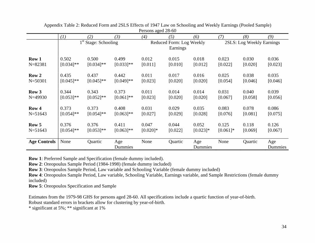
Appendix Table 2: Reduced Form and 2SLS Effects of 1947 Law on Schooling and Weekly Earnings (Pooled Sample) Persons aged 28-60
(1) (2) (3) (4) (5) (6) (7) (8) (9) 1st Stage: Schooling Reduced Form: Log Weekly
Earnings 2SLS: Log Weekly Earnings
Row 1 0.502 0.500 0.499 0.012 0.015 0.018 0.023 0.030 0.036 N=82381 [0.034]** [0.034]** [0.033]** [0.011] [0.010] [0.012] [0.022] [0.020] [0.023] Row 2 0.435 0.437 0.442 0.011 0.017 0.016 0.025 0.038 0.035 N=50301 [0.045]** [0.045]** [0.049]** [0.023] [0.020] [0.020] [0.054] [0.046] [0.046] Row 3 0.344 0.343 0.373 0.011 0.014 0.014 0.031 0.040 0.039 N=49930 [0.053]** [0.052]** [0.061]** [0.023] [0.020] [0.020] [0.067] [0.058] [0.056] Row 4 0.373 0.373 0.408 0.031 0.029 0.035 0.083 0.078 0.086 N=51643 [0.054]** [0.054]** [0.063]** [0.027] [0.029] [0.028] [0.076] [0.081] [0.075] Row 5 0.376 0.376 0.411 0.047 0.044 0.052 0.125 0.118 0.126 N=51643 [0.054]** [0.053]** [0.063]** [0.020]* [0.022] [0.023]* [0.061]* [0.069] [0.067] Age Controls None Quartic Age
Dummies None Quartic Age
Dummies None Quartic Age
Dummies Row 1: Preferred Sample and Specification (female dummy included). Row 2: Oreopoulus Sample Period (1984-1998) (female dummy included) Row 3: Oreopoulos Sample Period, Law variable and Schooling Variable (female dummy included) Row 4: Oreopoulos Sample Period, Law variable, Schooling Variable, Earnings variable, and Sample Restrictions (female dummy included) Row 5: Oreopoulos Specification and Sample Estimates from the 1979-98 GHS for persons aged 28-60. All specifications include a quartic function of year-of-birth. Robust standard errors in brackets allow for clustering by year-of-birth. * significant at 5%; ** significant at 1%
35
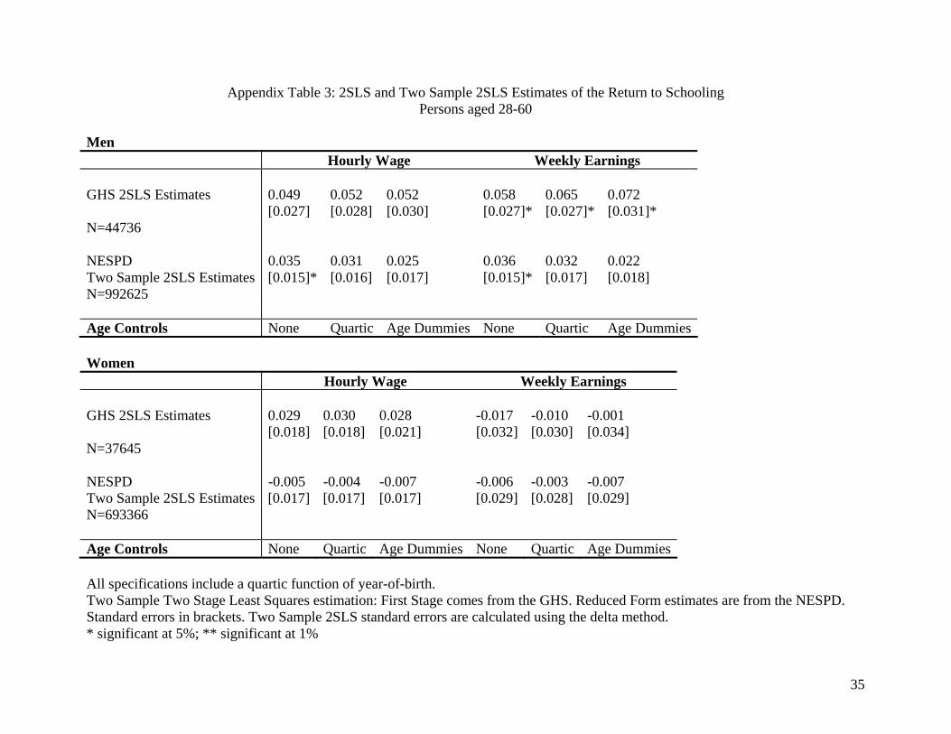
Appendix Table 3: 2SLS and Two Sample 2SLS Estimates of the Return to Schooling Persons aged 28-60
Men Hourly Wage Weekly Earnings GHS 2SLS Estimates 0.049 0.052 0.052 0.058 0.065 0.072 [0.027] [0.028] [0.030] [0.027]* [0.027]* [0.031]* N=44736 NESPD 0.035 0.031 0.025 0.036 0.032 0.022 Two Sample 2SLS Estimates [0.015]* [0.016] [0.017] [0.015]* [0.017] [0.018] N=992625 Age Controls None Quartic Age Dummies None Quartic Age Dummies Women Hourly Wage Weekly Earnings GHS 2SLS Estimates 0.029 0.030 0.028 -0.017 -0.010 -0.001 [0.018] [0.018] [0.021] [0.032] [0.030] [0.034] N=37645 NESPD -0.005 -0.004 -0.007 -0.006 -0.003 -0.007 Two Sample 2SLS Estimates [0.017] [0.017] [0.017] [0.029] [0.028] [0.029] N=693366 Age Controls None Quartic Age Dummies None Quartic Age Dummies All specifications include a quartic function of year-of-birth. Two Sample Two Stage Least Squares estimation: First Stage comes from the GHS. Reduced Form estimates are from the NESPD. Standard errors in brackets. Two Sample 2SLS standard errors are calculated using the delta method. * significant at 5%; ** significant at 1%
36
Figure 1: Proportion of Women Leaving School by Age 14 (GHS)
0.2
.4.6
.8P
ropo
rtion
Lea
ving
Sch
ool b
y A
ge 1
4
25 30 35 40 45 50Birth Cohort
Local Average Polynomial Fit
Figure 2: Proportion of Men Leaving School by Age 14 (GHS)
0.2
.4.6
.8P
ropo
rtion
Lea
ving
Sch
ool b
y A
ge 1
4
25 30 35 40 45 50Birth Cohort
Local Average Polynomial Fit
37
Figure 3: Average School Leaving Age by Year-of-Birth for Women (GHS)
14.5
1515
.516
Ave
rage
Sch
ool-L
eavi
ng A
ge
25 30 35 40 45 50Birth Cohort
Local Average Polynomial Fit
Figure 4: Average School Leaving Age by Year-of-Birth for Men (GHS)
14.5
1515
.516
Ave
rage
Sch
ool-L
eavi
ng A
ge
25 30 35 40 45 50Birth Cohort
Local Average Polynomial Fit
38
Figure 5: Average Hourly Wage by Year-of-Birth for Women (GHS)
1.4
1.5
1.6
1.7
1.8
Ave
rage
Log
Hou
rly W
age
25 30 35 40 45 50Birth Cohort
Local Average Polynomial Fit
Figure 6: Average Hourly Wage by Year-of-Birth for Men (GHS)
1.9
22.
12.
2
Aver
age
Log
Hou
rly W
age
25 30 35 40 45 50Birth Cohort
Local Average Polynomial Fit
39
Figure 7: Average Hourly Wage by Year-of-Birth for Women (NESPD)
1.65
1.7
1.75
1.8
1.85
Ave
rage
Log
Hou
rly W
age
25 30 35 40 45 50Birth Cohort
Local Average Polynomial Fit
Figure 8: Average Hourly Wage by Year-of-Birth for Men (NESPD)
22.
052.
12.
152.
2
Ave
rage
Log
Hou
rly W
age
25 30 35 40 45 50Birth Cohort
Local Average Polynomial Fit
40
Figure 9: Average Weekly Earnings by Year-of-Birth for Women (GHS and CHS)
77.
58
8.5
Ave
rage
Log
Wee
kly
Ear
ning
s
25 30 35 40 45 50Birth Cohort
Britain Northern Ireland
Figure 10: Average Weekly Earnings by Year-of-Birth for Men (GHS and CHS)
8.5
99.
5A
vera
ge L
og W
eekl
y E
arni
ngs
25 30 35 40 45 50Birth Cohort
Britain Northern Ireland