Compressed Sensing for Wireless Communications : Useful ... · Compressed Sensing for Wireless Communications : Useful Tips and Tricks ... it is not easy to come up with simple and

arX

iv:1

511.

0874

6v2

[cs.

IT]

10 M

ay 2

016

Compressed Sensing for Wireless

Communications : Useful Tips and Tricks

Jun Won Choi∗, Byonghyo Shim, Yacong Ding, Bhaskar Rao, Dong In Kim†

∗Hanyang University, Seoul, Korea

Seoul National University, Seoul, Korea

University of California at San Diego, CA, USA

†Sungkyunkwan University, Suwon, Korea

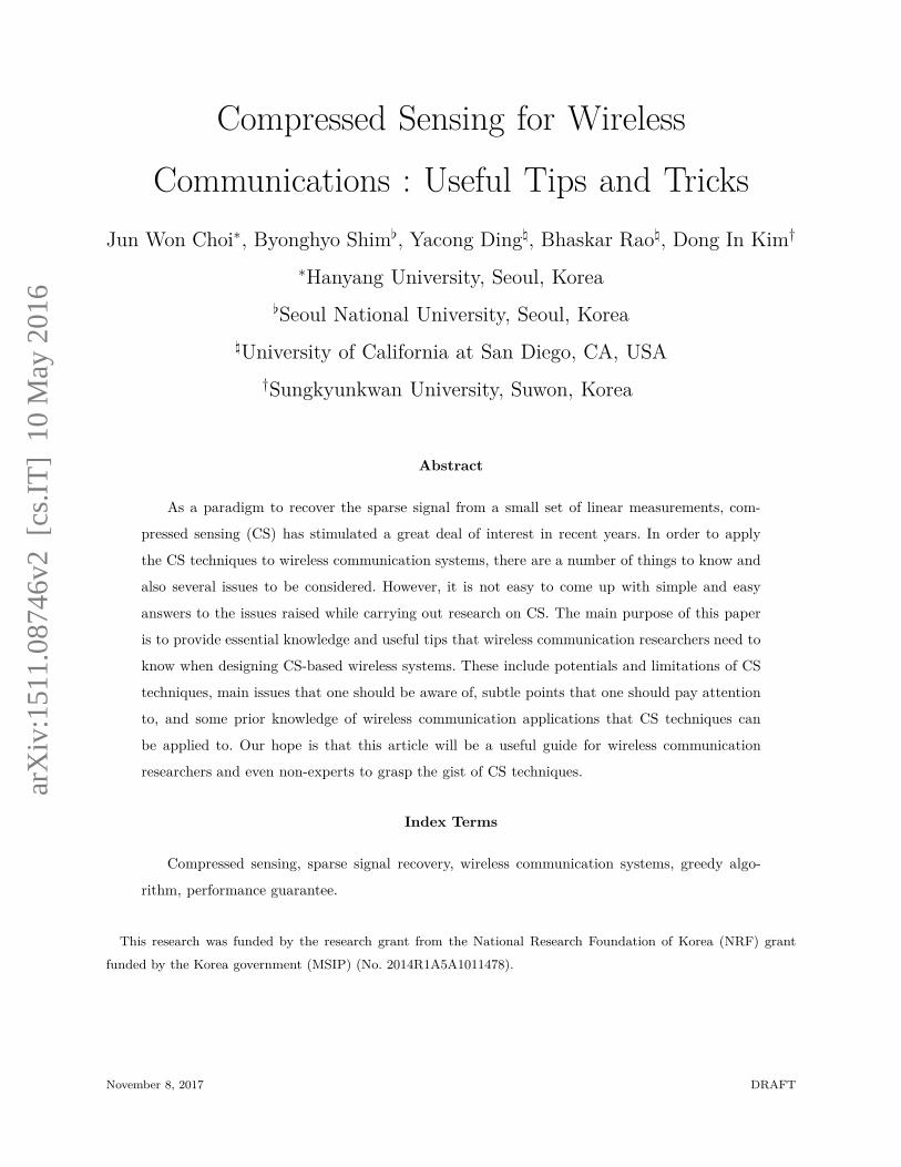
Abstract

As a paradigm to recover the sparse signal from a small set of linear measurements, com-

pressed sensing (CS) has stimulated a great deal of interest in recent years. In order to apply

the CS techniques to wireless communication systems, there are a number of things to know and

also several issues to be considered. However, it is not easy to come up with simple and easy

answers to the issues raised while carrying out research on CS. The main purpose of this paper

is to provide essential knowledge and useful tips that wireless communication researchers need to

know when designing CS-based wireless systems. These include potentials and limitations of CS

techniques, main issues that one should be aware of, subtle points that one should pay attention

to, and some prior knowledge of wireless communication applications that CS techniques can

be applied to. Our hope is that this article will be a useful guide for wireless communication

researchers and even non-experts to grasp the gist of CS techniques.

Index Terms

Compressed sensing, sparse signal recovery, wireless communication systems, greedy algo-

rithm, performance guarantee.

This research was funded by the research grant from the National Research Foundation of Korea (NRF) grant

funded by the Korea government (MSIP) (No. 2014R1A5A1011478).

November 8, 2017 DRAFT

http://arxiv.org/abs/1511.08746v2

1

I. Introduction

Compressed sensing (CS) is an attractive paradigm to acquire, process, and recover

the sparse signals [1]. This new paradigm is very competitive alternative to conventional

information processing operations including sampling, sensing, compression, estimation, and

detection. The traditional way to acquire and reconstruct analog signals from sampled signal

is based on the celebrated Nyquist-Shannon’s sampling theorem [2] which states that the

sampling rate should be at least twice the bandwidth of an analog signal to restore it from

the discrete samples accurately. In case of discrete signal regime, the fundamental theorem

of linear algebra states that the number of observations in a linear system should be at

least equal to the length of the desired signal to ensure the accurate recovery of the desired

signal. While these fundamental principles hold true always, it might be too stringent in a

situation where signals of interest are sparse, meaning that the signals can be represented

using a relatively small number of nonzero coefficients.

The CS paradigm provides a new perspective on the way we process the information. In

essence, key premise of the CS is that a small number of linear measurements (projections)

of the signal contain enough information for its reconstruction. Main wisdom behind the

CS is that essential knowledge in the large dimensional signals is just handful, and thus

measurements with the size being proportional to the sparsity level of the input signal is

enough to reconstruct the original signal. In fact, in many real-world applications, signals

of interest are sparse or can be approximated as a sparse vector in a properly chosen basis.

Sparsity of underlying signals simplifies the acquisition process, reduces memory requirement

and computational complexity, and further enables to solve the problem which has been

believed to be unsolvable.

In the last decade, CS techniques have spread rapidly in various disciplines such as medical

imaging, machine learning, computer science, statistics, and many others. When compared

to these disciplines, dissemination of CS techniques to wireless communications industry

seems to be relatively slow. These days, many tutorials, textbooks, and papers are available

[4]–[6], but it might not be easy to grasp the essentials and useful tips tailored for wireless

communication engineers. Thus, CS remains somewhat esoteric and vague field for many

wireless communication researchers who want to grasp the gist of CS to use it in their


2

applications. Notwithstanding the foregoing, much of the fundamental principle and basic

knowledge is simple, intuitive, and easy to understand.

The purpose of this paper is not to describe the complicated mathematical expressions

required for the characterization of the CS, nor to describe the details of state-of-the-art

CS techniques and sparse recovery algorithms, but to bridge the gap between the wireless

communications and CS principle by providing essentials and useful tips and tricks that

communication engineers and researchers need to be aware of. With this purpose in mind, we

organized this article as follows. In Section II, we provide an overview of basics of compressed

sensing. We review how to solve the systems with linear equations for both overdetermined

and underdetermined systems and then move on to the scenario where the input vector is

sparse in the underdetermined setting. In Section III, we describe the basic system model

for the wireless communication systems and then introduce the CS problems related to

wireless communications. Depending on the sparse structure of the desired signal vector,

CS problems can be divided into four sub-problems: sparse estimation, sparse detection,

support identification, and non-sparse detection problems. We discuss each problem with the

specific wireless communication applications. Developing successful CS technique for the

specific wireless application requires good understanding on key issues (e.g., properties of

system matrix and input vector, algorithm selection/modification/design, system setup and

performance requirements). In Section IV, we go over main issues in a way of answering to

seven fundamental questions. In each issue, we provide useful tips, benefits and limitations,

and essential knowledge so that readers can catch the gist and thus take advantage of

CS techniques. We conclude the paper in Section V by summarizing the contributions and

discussing open issues down the road. Our hope is that this paper will provide better view and

understanding of the potentials and limitations of CS techniques to wireless communication

researchers.

In the course of this writing, we observe a large body of researches on CS, among which

we briefly summarize some notable tutorial and survey results here. Short summary of CS

is presented by Baraniuk [3]. Extended summary can be found in Candes and Wakin [4].

Forucart and Rauhut provided a tutorial of CS with an emphasis on mathematical properties

for performance guarantee [7] and similar approach can be found in [8]. Comprehensive

treatment on various issues, such as sparse recovery algorithms, performance guarantee, and


3

CS applications, can be found in the book of Eldar and Kutyniok [5]. Book of Han, Li,

and Yin summarized the CS techniques for wireless network applications [6] and Hayashi,

Nagahara, and Tanaka discussed the applications of CS to the wireless communication

systems [9].

II. Basics of Compressed Sensing

A. Solutions of Linear Systems

We begin with a linear system having m equations and n unknowns given by

y = Hs (1)

where y is the measurement vector, s is the desired signal vector to be reconstructed, and

H ∈ Rm×n is the system matrix. In this case, the measurement vector y can be expressed

as a linear combination of the columns of H, that is, y =∑

i sihi (si and hi are the i-th

entry of s and i-th column of H, respectively) so that y lies in the subspace spanned by the

columns of H.

We first consider the scenario where the number of measurements is larger than or equal

to the size of unknown vector (m ≥ n). In this case, often referred to as overdetermined

scenario, one can recover the desired vector s using a simple algorithm (e.g., Gaussian

elimination) as long as the system matrix is a full rank (i.e., rank(H) = minm,n). Even

if this is not the case, one can find an approximate solution minimizing the error vector

e = y − Hs. The vector s∗ minimizing the ℓ2-norm of the error vector is

s∗ = arg mins

‖e‖2. (2)

Since ‖e‖22 = sT HT Hs − 2yT Hs + yT y, by setting the derivative of ‖e‖2

2 with respect to s

to zero, we have ∂∂s

‖e‖22 = 2HT Hs − 2HT y = 0, and

s∗ = (HT H)−1HT y. (3)

The obtained solution s∗ is called least squares solution and the operator (HT H)−1HT is

called the pseudo inverse and denoted as H†. Note that Hs∗ is closest to the measurement

vector y among all possible points in the range space of H.

While finding the solution in an overdetermined scenario is straightforward and fairly

accurate in general, the task to recover the input vector in an underdetermined scenario


4

where the measurement size is smaller than the size of unknown vector (m < n) is challenging

and problematic, since one cannot find out the unique solution general. As a simple example,

consider the example where H = [1 1] and the original vector is s = [s1 s2]T = [1 1]T (and

hence y = 2). Since the system equation is 2 = s1 + s2, one can easily observe that there

are infinitely many possible solutions. This is because for any vector v = [v1 v2]T satisfying

0 = v1 + v2 (e.g., v1 = −1 and v2 = 1), s′ = s + v also satisfies y = Hs′. Indeed, there are

infinitely many vectors in the null space N(H) = v | Hv = 0 for the underdetermined

scenario so that one cannot find out the unique solution satisfying (1). In this scenario,

because HT H is not full rank and hence non-invertible, one cannot compute the least squares

solution in (3). Alternative approach is to find a solution minimizing the ℓ2-norm of s while

satisfying y = Hs:

s∗ = arg min ‖s‖2 s.t. y = Hs. (4)

Using the Lagrangian multiplier method, one can obtain1

s∗ = HT (HHT )−1y. (5)

Since the solution s∗ is a vector satisfying the constraint (y = Hs) with the minimum

energy, it is often called minimum norm solution. Since the system has more unknowns

than measurements, the minimum norm solution in (5) cannot guarantee to recover the

original input vector. This is well-known bad news. However, as we will see in the next

subsection, sparsity of the input vector provides an important clue to recover the original

input vector.

B. Solutions of Underdetermined Systems for Sparse Input Vector

As mentioned, underdetermined system has infinitely many solutions. If one wish to

narrow down the choice to convert ill-posed problem into well-posed one, additional hint

(side information) is needed. In fact, CS principle exploits the fact that the desired signal

vector is sparse in finding the solution. A vector is called sparse if the number of nonzero

1By setting derivative of the Lagrangian L(s, λ) = ‖s‖2

2 + λT (y − Hs) with respective to s to zero, we obtain

s∗ = − 1

2HT λ. Using this together with y = Hs, we get λ = −2(HHT )−1y and s∗ = HT (HHT )−1y.


5

Fig. 1. Illustration of ℓ0,ℓ1, and ℓ2-norm minimization approach. If the sparsity of the original vector s is one, then

s is in the coordinate axes.

entries is sufficiently smaller than the dimension of the vector. As a metric to check the

sparsity, we use ℓ0-norm ‖s‖0 of a vector s, which is defined as2

‖s‖0 = #i : si 6= 0.

For example, if s = [3 0 0 0 1 0], then ‖s‖0 = 2. In the simple example we discussed

(2 = s1 + s2), if s = [s1 s2] is sparse, then at least s1 or s2 needs to be zero (i.e., s1 = 0 or

s2 = 0). Interestingly, by invoking the sparsity constraint, the number of possible solutions

is dramatically reduced from infinity to two (i.e., (s1, s2) = (2, 0) or (0, 2)).

Since the ℓ0-norm is the sparsity promoting function, the problem to find the sparest

input vector from the measurement vector is readily expressed as

s∗ = arg min ‖s‖0 s.t. y = Hs. (6)

Since the ℓ0-norm counts the number of nonzero elements in s, one should rely on the

combinatoric search to get the solution in (6). In other words, all possible subsystems y =

HΛsΛ is investigated, where HΛ is the submatrix of H that contains columns indexed by Λ.3

2One can alternatively define as ‖s‖0 = limp→0 ‖s‖pp = limp→0

∑

i|si|

p

3For example, if Λ = 1, 3, then HΛ = [h1 h3].


6

Initially, we investigate the solution with the sparsity one by checking y = hisi for each i. If

the solution is found (i.e., a scalar value si satisfying y = hisi is found), then the solution

s∗ = [0 · · · 0 si 0 · · · 0] is returned and the algorithm is finished. Otherwise, we investigate

the solution with the sparsity two by checking if the measurement vector is constructed by

a linear combination of two columns of H. This step is repeated until the solution satisfying

y = HΛsΛ is found. Since the complexity of this exhaustive search increases exponentially

in n, ℓ0-norm minimization approach is impractical in most real-world applications.

Alternative approach suggested by Donoho [1] and Candes and Tao [4] is ℓ1-norm mini-

mization approach given by

s∗ = arg min ‖s‖1 s.t. y = Hs. (7)

While the ℓ1-norm minimization problem in (7) lies in the middle of (6) and (4), it can

be cast into the convex optimization problem so that the solution of (7) can be obtained

by the standard linear programming (LP) [1]. In Fig. 1, we illustrate ℓ0, ℓ1 and ℓ2-norm

minimization techniques. If the original vector is sparse (say the sparsity is one), then the

desired solution can be found by the ℓ0-norm minimization since the points being searched

are those in the coordinate axes (sparsity one). Since ℓ1-norm has a diamond shape (it is in

general referred to as cross-polytope), one can observe from Fig. 1(b) that the solution of

this approach corresponds to the vertex, not the face of the cross-polytope in most cases.

Since the vertex of the diamond lies on the coordinate axes, it is highly likely that the ℓ1-

norm minimization technique returns the desired sparse solution. In fact, it has been shown

that under the mild condition the solution of ℓ1-norm minimization problem is identical to

the original vector [4]. Whereas, the solution of the ℓ2-norm minimization corresponds to

the point closest to the origin among all points s satisfying y = Hs so that the solution

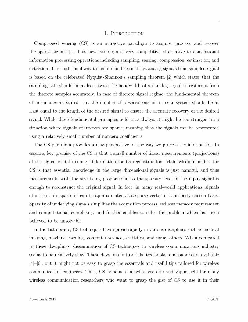
has no special reason to be placed at the coordinate axes. Thus, as depicted in Fig. 2, the

ℓ1-norm minimization solution is very close to the original sparse signal while the ℓ2-norm

minimization solution is far from being close.

We also note that when the measurement vector y is corrupted by the noise, one can

modify the equality constraint as

s∗ = arg min ‖s‖1 s.t. ‖y − Hs‖2 < ǫ (8)


7

0 10 20 30 40 50 60−2

−1

0

1

2

3

4

5

6

7

8

n

Original sparse vector

L1−norm minimization

L2−norm minimization

Fig. 2. Illustration of performance of ℓ1 and ℓ2-norm minimization techniques. Entries of the system matrix H ∈

R16×64 are chosen from standard Gaussian and the sparsity of s is set to 5.

where ǫ is a pre-determined noise level. This type of problem is often called basis pursuit

de-noising (BPDN) [40]. This problem has been well-studied subject in convex optimization

and there are a number of approaches to solve the problem (e.g., interior-point method [43]).

Nowadays, there are many optimization packages (e.g., CVX [41] or L1-magic [42]) so that

one can save the programming effort by using these software tools.

C. Greedy algorithm

While the LP technique to solve ℓ1-norm minimization problem is effective in recon-

structing the sparse vector, it requires computational cost, in particular for large-scale

applications. For example, a solver based on the interior point method has an associated

computational complexity order of O(m2n3) [1]. For many real-time applications including

wireless communication applications, therefore, computational cost and time complexity of

ℓ1-norm minimization solver might be burdensome.

Over the years, many algorithms to recover the sparse signals have been proposed. Notable

one among them is a greedy algorithm. By the greedy algorithm, we mean an algorithm to


8

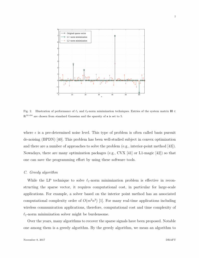
Fig. 3. Principle of the greedy algorithm. If the right columns are chosen, then the we can convert an underdetermined

system into an overdetermined system.

make a local optimal selection at each time with a hope to find the global optimum solution

in the end. Perhaps the most popular greedy algorithm is the orthogonal matching pursuit

(OMP) [45]. In the OMP algorithm, a column of the matrix H is chosen one at a time using

a greedy strategy. Specifically, in each iteration, a column maximally correlated with the

(modified) observation is chosen. Obviously, this is not necessarily optimal since the choice

does not guarantee to pick the column associated with the nonzero element of s. Let hπi

be the column chosen in the i-th iteration, then the (partial) estimate of s is si = H†iy and

the estimate of y is yi = Hisi where Hi = [hπ1hπ2

· · · hπi]. By subtracting yi from y,

we obtain the modified observation, denoted by ri and called the residual, used in the next

iteration (i.e., ri = y − yi). By removing the contribution of si from the observation vector

y so that we focus on the identification of the rest nonzero elemenets in the next iteration.

One can observe that when the column selection is right, the OMP algorithm can re-

construct the original sparse vector accurately. This is because columns corresponding to

the zero element in s can be removed from the system model so that the underdetermined

system can be converted into overdetermined system (see Fig. 3). As mentioned, the least

squares solution for the overdetermined system generates an accurate estimate of the original

sparse vector. Since the computational complexity is typically much smaller than that of

the LP techniques to solve (7) or (8), the greedy algorithm has received much attention


9

in recent years. Interestingly, even for the simple greedy algorithm like OMP algorithm,

recent results show that the recovery performance is comparable to the LP technique while

obsessing much lower computational overhead. We will discuss more on the sparse recovery

algorithm in Section IV-D.

D. Performance Guarantee

In order to analyze the performance guarantee of the sensing matrix and the sparse

recovery algorithm, many analysis tools have been suggested. For the sake of completeness,

we briefly go over some of these tools here. First, a simple yet intuitive property is the spark

of the matrix H. Spark of a matrix H is defined as the smallest number of columns of H

that are linearly dependent. From this definition, we see that a vector v in a null space

N(H) = v | Hv = 0 should satisfy ‖v‖0 ≥ spark(H) since a vector v in the null space

linearly combines columns in H to make the zero vector, and at least spark(H) columns are

needed to do so. Following results provide the minimum level of spark over which uniqueness

of the k-sparse solution is ensured.

Theorem 1 (Corollary 1 [4]): There is at most one k-sparse solution for a system of linear

equations y = Hs if and only if spark(H) > 2k.

Proof: See Appendix A

From the definition, it is clear that 1 ≤ spark(H) ≤ n + 1. If entries of H are i.i.d.

random, then no m columns in H would be linearly dependent with high probability so that

spark(H) = m+1. Using this together with Theorem 1, one can observe that the uniqueness

is guaranteed for every solution satisfying k ≤ m2

.

It is worth mentioning that it is not easy to compute the spark of a matrix since it requires

a combinatoric search over all possible subsets of columns in H. Thus, it is preferred to use a

property that is easily computable. A tool that meets this purpose is the mutual coherence.

The mutual coherence µ(H) is defined as the largest magnitude of normalized inner product

between two distinct columns of H:

µ(H) = maxi6=j

| < hi,hj > |‖hi‖2‖hj‖2

. (9)

In [46], it has been shown that for a full rank matrix, µ(H) satisfies

1 ≥ µ(H) ≥√

n−m

m(n − 1).


10

In particular, if n ≫ m, we obtain an approximate lower bound as µ(H) ≥ 1√m

. It has been

shown that µ(H) is related to spark(H) via spark(H) ≥ 1 + 1µ(H)

[47]. Using this together

with Theorem 1, we get the following uniqueness condition.

Theorem 2 (Corollary 1 [4]): If k < 12(1 + 1

µ(H)), then for each measurement vector, there

exists at most one k-sparse signal s satisfying y = Hs.

While the mutual coherence is relatively easy to compute, the bound obtained from this is

too strict in general. These days, restricted isometry property (RIP), introduced by Candes

and Tao [39], has been used as a popular tool to establish the performance guarantee.

Definition 3: A system matrix H is said to satisfy the restricted isometry property (RIP)

if for all K-sparse vector s, the following condition holds

(1 − δ)‖s‖22 ≤ ‖Hs‖2

2 ≤ (1 + δ)‖s‖22. (10)

In particular, the smallest δ, denoted as δk is referred to as a RIP constant. In essence,

δk indicates how well the system matrix preserves the energy of the original signal. On

one hand, if δk ≈ 0, the system matrix is close to orthonormal so that the reconstruction

of s would be guaranteed almost surely with a simple matching filtering operation (e.g.,

s = HHy). On the other hand, if δk ≈ 1, it might be possible that ‖Hs‖22 ≈ 0 (i.e., s is in

the nullspace of H) so that the measurements y = Hs may not preserve any information

on s. In this case, obviously, the recovery of s would be nearly impossible.

Note that RIP is useful to analyze performance when the measurements are contaminated

by the noise [4], [48], [49], [51]. Additionally, by the help of random matrix theory, one

can perform probabilistic analysis when the entries of the system matrix are i.i.d. random.

Specifically, it has been shown that many random matrices (e.g., random Gaussian, Bernoulli,

and partial Fourier matrices) satisfy the RIP with exponentially high probability, when the

number of measurements scales linearly in the sparsity level [5]. As a well-known example,

if δ2k <√

2 − 1, then the solution in (7) obeys

‖s∗ − s‖2 ≤ C0‖s − sk‖1/√k (11)

‖s∗ − s‖1 ≤ C0‖s − sk‖1 (12)

for some constant C0, where sk is the vector s with all but the largest k components set

to 0. It shows that if s is k-sparse, then s = sk, and thus the recovery is exact. If s is not


11

k-sparse, then quality of recovery is limited by the difference of the true signal s and its best

k approximation sk. For a signal which is not exact sparse but can be well approximated by a

k-sparse signal (i.e., ‖s−sk‖1 is small), we can still achieve fairly good recovery performance.

While the performance guarantees obtained by RIP or other tools provide a simple

characterization of system parameters (number of measurements, system matrix, algorithm)

for the recovery algorithm, these results need to be taken with a grain of salt, in particular

when designing the practical wireless systems. This is because the performance guarantee,

expressed as a sufficient condition, might be loose and working in asymptotic sense in many

cases. Also, some of them are, in the wireless communications perspective, based on too

stringent assumptions (e.g., Gaussianity of the system matrix, strict sparsity of input vector).

Further, it is very difficult to check whether the system setup satisfies the recovery condition

or not.4

III. Compressed Sensing for Wireless Communications

A. System Model

In this section, we describe four distinct CS problems relating to the wireless communica-

tions. We begin with the basic system model where transmission of signals is performed over

linear channels with additive white Gaussian noise (AWGN). The input-output relationship

in this model is

y = Hs + v, (13)

where y is the vector of received signals, H ∈ Cm×n is the system matrix,5 s is the desired

signal vector we want to recover, and v is the noise vector (v ∼ CN (0, σ2I)). In this article,

we are primarily interested in the scenario where the desired vector s is sparse, meaning that

the portion of nonzero entries in s is far smaller than its dimension. It is worth mentioning

that even when the desired vector is non-sparse, one can either approximate it to a sparse

vector or convert it to the sparse vector using a proper transform. For example, when the

magnitude of nonzero elements is small, we can obtain an approximately sparse vector by

4For example, one need to check(

n

2k

)

submatrices of H to identify the RIP constant δ2k.

5In the compressed sensing literatures, y and H are referred to as measurement vector and sensing matrix (or

measurement matrix), respectively.


12

ignoring negligible nonzero elements. For example, if s = [2 0 0 0 0 3 0.1 0.05 0.01 0]T ,

then we can approximate it to 2-sparse vector s′ = [2 0 0 0 0 3 0 0 0 0]T . In this case, the

effective system model would be y = Hs′ + v′ where v′ = Hνsν + v (Hν = [h7 h8 h9] and

sν = [0.1 0.05 0.01]T ). Also, even in the case where the desired vector is not sparse, one

might choose proper basis ψi to express the signal as a linear combination of basis. In

the image/video processing society, for example, discrete Fourier transform (DFT), discrete

cosine transform (DCT) , and wavelet transform have long been used. Using a properly

chosen basis matrix Ψ = [ψ1 · · · ψn], input vector can be expressed as s =∑

i xiψi = Ψx

and thus

y = Hs + v = HΨx + v, (14)

where x is a representation of s in Ψ domain. By the proper choice of the basis, one can

convert the original non-sparse vector s into the sparse vector x. Since this new represen-

tation does not change the system model, in the sequel we will use a standard model in

(13).

Depending on the way the desired vector is constructed, the CS-related problem can be

classified into several distinctive subproblems.

B. Sparse Estimation

When the signal vector is sparse and its nonzero element is real (or complex), the problem

to recover s from y is classified into sparse estimation problem. Sparse estimation problem

is popular and often regarded as a synonym of sparse signal recovery problem.

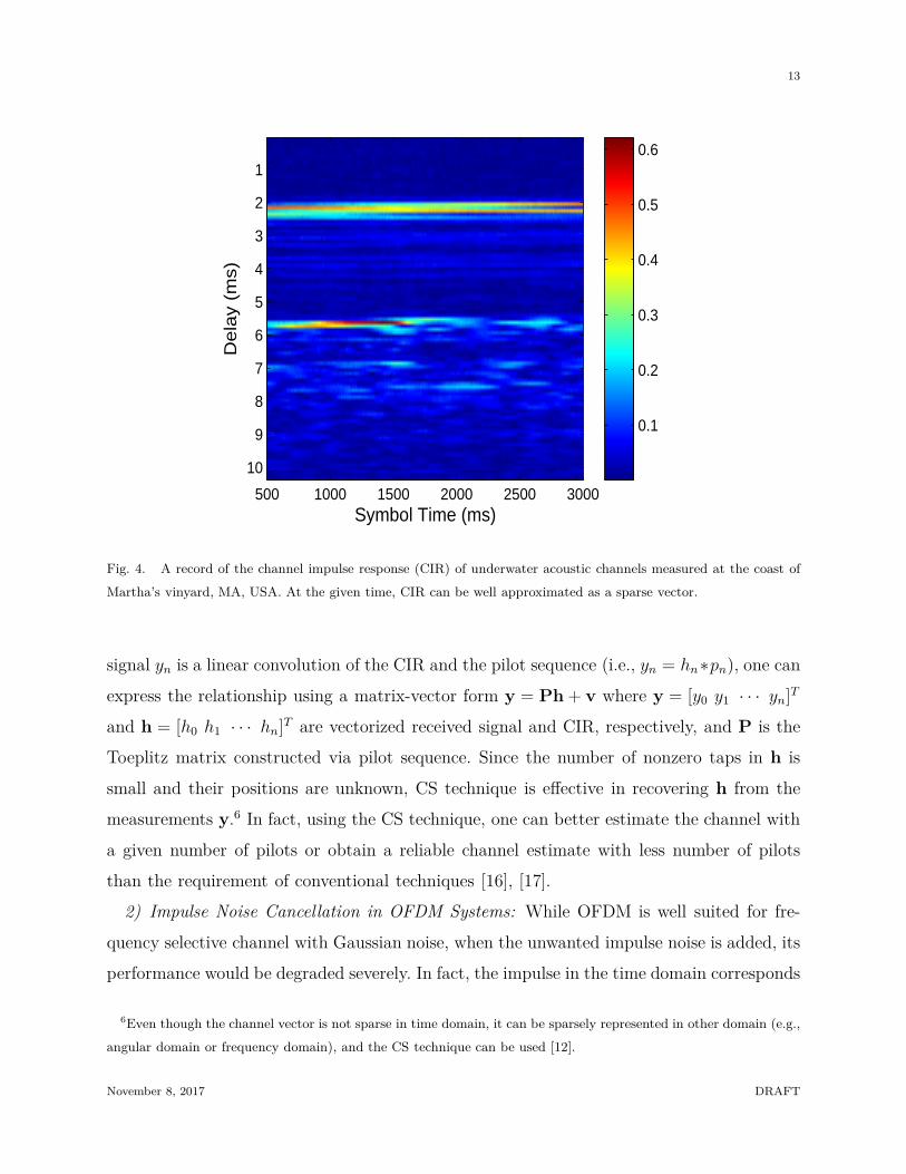
1) Channel Estimation: Channel estimation is a typical example of the sparse estimation.

In many wireless channels, such as ultra-wideband (UWB), underwater acoustic (UWA), or

millimeter wave (mmWave) channels, delay spread is larger than the number of significant

paths and hence the channel vector can be well approximated as a sparse signal [10]–[14]

(e.g., see Fig. 4). Even for the cellular environment (e.g., extended vehicular-A (EVA) or

extended typical urban (ETU) channel model in LTE systems [15]), time-domain channel

impulse responses (CIR) are well modeled as a sparse vector since only a few channel paths

are dominant. In the channel estimation problem, the system matrix is constructed via

known transmit signals referred to as pilot signals (or training signals). Since the received


13

Symbol Time (ms)

De

lay

(ms)

500 1000 1500 2000 2500 3000

1

2

3

4

5

6

7

8

9

10

0.1

0.2

0.3

0.4

0.5

0.6

Fig. 4. A record of the channel impulse response (CIR) of underwater acoustic channels measured at the coast of

Martha’s vinyard, MA, USA. At the given time, CIR can be well approximated as a sparse vector.

signal yn is a linear convolution of the CIR and the pilot sequence (i.e., yn = hn∗pn), one can

express the relationship using a matrix-vector form y = Ph + v where y = [y0 y1 · · · yn]T

and h = [h0 h1 · · · hn]T are vectorized received signal and CIR, respectively, and P is the

Toeplitz matrix constructed via pilot sequence. Since the number of nonzero taps in h is

small and their positions are unknown, CS technique is effective in recovering h from the

measurements y.6 In fact, using the CS technique, one can better estimate the channel with

a given number of pilots or obtain a reliable channel estimate with less number of pilots

than the requirement of conventional techniques [16], [17].

2) Impulse Noise Cancellation in OFDM Systems: While OFDM is well suited for fre-

quency selective channel with Gaussian noise, when the unwanted impulse noise is added, its

performance would be degraded severely. In fact, the impulse in the time domain corresponds

6Even though the channel vector is not sparse in time domain, it can be sparsely represented in other domain (e.g.,

angular domain or frequency domain), and the CS technique can be used [12].


14

to the constant in the frequency domain, very strong time domain impulses will give negative

impact to most of frequency domain symbols. Since the span of impulse noise is short in time

and thus can be considered as a sparse vector, we can apply the CS technique to mitigate

this noise [18]. First, the discrete time complex baseband equivalent channel model for the

OFDM signal is expressed as

y = Hxt + n (15)

where y and xt are the time-domain receive and transmit signal blocks (after the cyclic

prefix removal), H is the circulant matrix (generated by the cyclic prefix), and n is additive

Gaussian noise vector. When the impulse noise e is added, the received signal vector becomes

y = Hxt + e + n. (16)

Note that the circulant matrix can be eigen-decomposed by the DFT matrix F (i.e.,

H = FHΛF) [19]. Also, the time-domain transmit signal in OFDM systems is expressed as

xt = FHxf = FHΠs where xf is the frequency-domain symbol vector, Π is n × q selection

matrix containing only one element being one in each column and rest being zero, and s is

frequency-domain symbol vector of dimension q ≤ n. Thus, (16) can be rewritten as

y = (FHΛF)(FHΠs) + e + n

= FHΛΠs + e + n. (17)

Let y′ be the received vector after the DFT operation (y′ = Fy). Then, we have

y′ = ΛΠs + Fe + n′ (18)

where n′ = Fn is also Gaussian having the same statistic of n. In removing the impulse noise,

we use the subcarriers free of modulation symbols. By projecting y′ onto the space where

symbol is not allocated (i.e., orthogonal complement of the signal subspace), we obtain7

y′′ = Py′ = PFe + n′′ (19)

7As a simple example, if F is 4 × 4 DFT matrix and the first and third subcarrier is being used s =

[

s1

s3

]

, then

the selection matrix is Π =

1 0

0 0

0 1

0 0

and the projection operator is P =

0 0 0 0

0 1 0 0

0 0 0 0

0 0 0 1

.


15

where n′′ = Pn′ is the sub-sampled noise vector. Note that y′′ is a projection of n-dimensional

impulse noise vector onto a subspace of dimension m(≪ n). Once the impulse noise estimate

e is generated from the CS technique, then we can subtract Fe from the received vector y′

so that we obtain the modified received vector

y′ = ΛΠs + F(e − e) + n′. (20)

This is clearly better than the observation without impulse noise cancellation in (18) so that

we can achieve the improved detection performance.

C. Sparse Detection

In recent years, internet of things (IoT), providing network connectivity of almost all

things at all times, has received much attention for its plethora of applications such as

healthcare, automatic metering, environmental monitoring (temperature, humidity, mois-

ture, pressure), surveillance, automotive systems, and many more [20]. Common feature of

the IoT networks is that the node density is much higher than the cellular network, yet the

data rate is very low and not every device transmits information at given time. Due to this

reason, when we consider the uplink of IoT networks, dimension of a transmit vector s (i.e.,

number of devices) is large but the number of nonzero elements of s (i.e., number of active

devices) is small so that the transmit vector s can be readily modeled as a sparse vector.

Furthermore, since the available time/frequency resources of IoT systems is limited due to

the limitation of bandwidth, cost of RF circuits and antenna, and power consumption,8 the

number of resources m is smaller than the number of total devices n. The corresponding

input-output relationship is y =∑n

i=1 hisi + v = Hs + v where hi ∈ Cm is the channel

vector from the device i to the basestation and H ∈ Cm×n is the overall channel matrix.

This problem is distinct from the sparse estimation problem in the sense that elements of

signal vector s are chosen either from the set of finite alphabets (when the device is active) or

zero (when the device is inactive). To distinguish this problem from the sparse estimation

8In fact, a duty cycle based energy management is required for IoT sensors whose power consumption is very small,

and hence they are sustainable by the energy harvesting from renewable resources, such as solar, wind, motion, and

RF signals. In this regard, CS technique fits well into the “opportunistic” harvesting and transmission of the IoT

sensors to meet the “bursty” energy and traffic arrivals, unlike the existing cellular network.


16

problem, we call this type of recovery problem as sparse detection problem. Traditional

way to handle this problem to treat all interfering signals as a noise. Denoting s1 as the

desired symbol, the system model for this approach is given by y = h1s1 + (∑

i6=i hisi + v)

where the quantities inside the parenthesis correspond to an effective noise (sum of noise

and interferences). This strategy is simple to implement but it is not so appealing since the

signal recovery operation is performed in a very low signal-to-interference-noise ratio (SINR)

regime (SINR =E‖hisi‖2

2∑

j 6=iE‖hisi‖2

2+σ2

v). Since s is a sparse vector, we can use the CS technique

exploiting the integer constraint as a side information to detect the signal under the better

SINR condition.

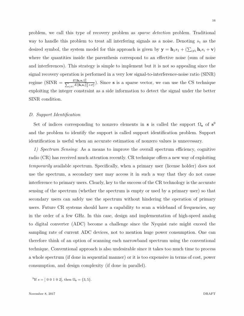
D. Support Identification

Set of indices corresponding to nonzero elements in s is called the support Ωs of s9

and the problem to identify the support is called support identification problem. Support

identification is useful when an accurate estimation of nonzero values is unnecessary.

1) Spectrum Sensing: As a means to improve the overall spectrum efficiency, cognitive

radio (CR) has received much attention recently. CR technique offers a new way of exploiting

temporarily available spectrum. Specifically, when a primary user (license holder) does not

use the spectrum, a secondary user may access it in such a way that they do not cause

interference to primary users. Clearly, key to the success of the CR technology is the accurate

sensing of the spectrum (whether the spectrum is empty or used by a primary user) so that

secondary users can safely use the spectrum without hindering the operation of primary

users. Future CR systems should have a capability to scan a wideband of frequencies, say

in the order of a few GHz. In this case, design and implementation of high-speed analog

to digital converter (ADC) become a challenge since the Nyquist rate might exceed the

sampling rate of current ADC devices, not to mention huge power consumption. One can

therefore think of an option of scanning each narrowband spectrum using the conventional

technique. Conventional approach is also undesirable since it takes too much time to process

a whole spectrum (if done in sequential manner) or it is too expensive in terms of cost, power

consumption, and design complexity (if done in parallel).

9If s = [ 0 0 1 0 2], then Ωs = 3, 5.


17

)(1 tp

)(tpi

)(tpm

)(th

)(th

)(th

][1 ny

][ nyi

][ nym

)(~1 ts

)(~ tsi

)(~ tsm

)(ts

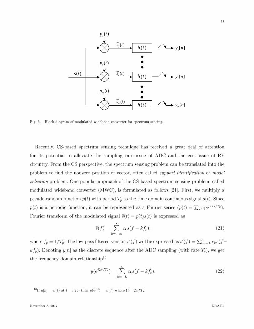
Fig. 5. Block diagram of modulated wideband converter for spectrum sensing.

Recently, CS-based spectrum sensing technique has received a great deal of attention

for its potential to alleviate the sampling rate issue of ADC and the cost issue of RF

circuitry. From the CS perspective, the spectrum sensing problem can be translated into the

problem to find the nonzero position of vector, often called support identification or model

selection problem. One popular approach of the CS-based spectrum sensing problem, called

modulated wideband converter (MWC), is formulated as follows [21]. First, we multiply a

pseudo random function p(t) with period Tp to the time domain continuous signal s(t). Since

p(t) is a periodic function, it can be represented as a Fourier series (p(t) =∑

k ckej2πk/Tp),

Fourier transform of the modulated signal s(t) = p(t)s(t) is expressed as

s(f) =∞∑

k=−∞cks(f − kfp), (21)

where fp = 1/Tp. The low-pass filtered version s′(f) will be expressed as s′(f) =∑L

k=−L cks(f−kfp). Denoting y[n] as the discrete sequence after the ADC sampling (with rate Ts), we get

the frequency domain relationship10

y(ej2πfTs) =L∑

k=−L

cks(f − kfp). (22)

10If u[n] = w(t) at t = nTs, then u(ejΩ) = w(f) where Ω = 2πfTs.


18

When this operation is done in parallel for different modulating functions pi(t) (i = 1, 2, · · · , m),

we have multiple measurements yi(ej2πfTs). After stacking these, we obtain

y = [y1(ej2πfTs) · · · ym(ej2πfTs)]T

and the corresponding matrix-vector form y = Hs where s = [s(f − Lfp) · · · s(f + Lfp)]T

and H is the measurement matrix relating y and s. Since the large portion of the spectrum

band is empty, s can be readily modeled as a sparse vector, and the task is summarized as a

problem to find s from y = Hs. Note that this problem is distinct from the sparse estimation

problem since an accurate estimation of nonzero values is unnecessary. Recalling that the

main purpose of the spectrum sensing is to identify the empty band and not the occupied

one, it would not be a serious problem to slightly increase the false alarm probability (by

false alarm we mean the spectrum is empty but decided as an occupied one). However,

special attention should be paid to avoid the misdetection probability since the penalty

would be severe when the occupied spectrum is falsely declared to be an empty one.

2) Detection of Angle of Arrival and Angle of Departure: Support identification problem

arises for the estimation of angle of arrival (AoA) and angle of departure (AoD) in mmWave

systems. As the carrier frequency increases up to tens or hundreds of GHz, transmit signal

power decays rapidly with distance and wireless channels exhibit a few strong multipaths

components caused by the small number of dominant scatterers. In fact, signal components

departing and arriving from particular angles are very few compared to the total number

of angular bins. When estimates of AoA and AoD are available, beamforming with high

directivity is desirable to overcome the path loss of mmWave wireless channels. In estimating

AoA and AoD, the sparsity of the channel in the angular domain is useful. When employing

the uniform linear array antennas, MIMO channels in the angular domain is expressed as

Ha = ArΦaAHt , (23)

where Ar = [ar(φ1), ..., ar(φN)], At = [at(φ1), ..., at(φN)], N is the number of total angular

bins, ar(φi) and at(φi) are the steering vectors corresponding to the i-th angular bin for

AoA and AoD, respectively, and Φa is the N × N path-gain matrix whose (i, j)th entry

contains the path gain from the jth angular bin for AoD to ith angular bin for AoA. Note

that due to the sparsity of the channel in the angular domain, only a few elements of Φa


19

are nonzero. The received signal is expressed as

r = Hax + n

= ArΦaAHt x + n

=N∑

i=1

N∑

i=j

ar(θi)at(θj)Hxφi,j + n

= Hs + n, (24)

where x is a vector of known transmitted symbols, H = [a1,1, ..., aN,1, ..., aN,N ], ai,j =

ar(θi)at(θj)Hx, s = [φT

1 , ..., φTN ]T , and φi is the ith column of Φa. Since indices of the nonzero

elements in s correspond to the AoA and AoD information and the number of these elements

are small, s is modeled by a sparse vector and the CS techniques becomes an effective means

to find the support of s.

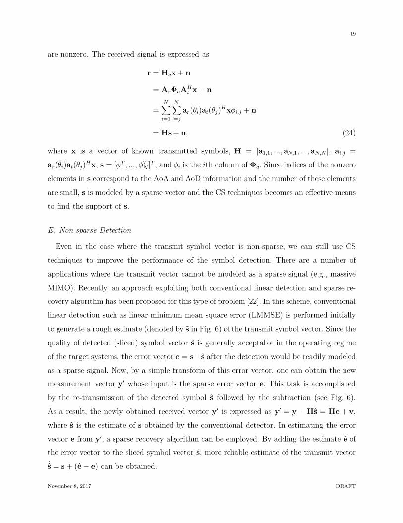
E. Non-sparse Detection

Even in the case where the transmit symbol vector is non-sparse, we can still use CS

techniques to improve the performance of the symbol detection. There are a number of

applications where the transmit vector cannot be modeled as a sparse signal (e.g., massive

MIMO). Recently, an approach exploiting both conventional linear detection and sparse re-

covery algorithm has been proposed for this type of problem [22]. In this scheme, conventional

linear detection such as linear minimum mean square error (LMMSE) is performed initially

to generate a rough estimate (denoted by s in Fig. 6) of the transmit symbol vector. Since the

quality of detected (sliced) symbol vector s is generally acceptable in the operating regime

of the target systems, the error vector e = s− s after the detection would be readily modeled

as a sparse signal. Now, by a simple transform of this error vector, one can obtain the new

measurement vector y′ whose input is the sparse error vector e. This task is accomplished

by the re-transmission of the detected symbol s followed by the subtraction (see Fig. 6).

As a result, the newly obtained received vector y′ is expressed as y′ = y − Hs = He + v,

where s is the estimate of s obtained by the conventional detector. In estimating the error

vector e from y′, a sparse recovery algorithm can be employed. By adding the estimate e of

the error vector to the sliced symbol vector s, more reliable estimate of the transmit vector

ˆs = s + (e − e) can be obtained.


20

Fig. 6. Using the sparse recovery algorithm, performance of non-sparse detection problem can be improved.

IV. Issues to Be Considered When Applying CS techniques to Wireless

Communication Systems

As more things should be considered in the design of wireless communication systems,

such as wireless channel environments, system configurations (bandwidth, power, number of

antennas), and design requirements (computation complexity, peak data rate, latency), the

solution becomes more challenging, ambitious, and complicated. As a result, applying the

CS techniques to wireless applications becomes not any more copy-and-paste type task and

one should have good knowledge of fundamental issues. Some of the questions that wireless

researchers can come across when they design a CS-based technique are listed as follows:

• Is sparsity important for applying CS technique? What is the desired sparsity level?

• How can we convert non-sparse vector into sparse one? Should we know sparsity a

priori?

• What is the desired property of the system matrix?

• What kind of recovery algorithms are there and what are pros and cons of these?

• What should we do if multiple observations are available?

• Can we do better if the input vector consists of finite alphabet symbols?

In this section, we go over these issues in a way of answering to these questions. In each

issue, we provide essential knowledge an useful tips and tricks for the successful development


21

of CS techniques for wireless communication systems.

A. Is Sparsity Important?

If you have an application that you think CS-based technique might be useful, then the

first thing to check is whether the signal vector to be recovered is sparse or not. Many natural

signals, such as image, sound, or seismic data are in themselves sparse or sparsely represented

in a properly chosen basis. Even though the signal is not strictly sparse, often it can be well

approximated as a sparse signal. For example, most of wireless channels exhibit power-law

decaying behavior due to the physical phenomena of waves (e.g., reflection, diffraction, and

scattering) so that the received signal is expressed as a superposition of multiple attenuated

and delayed copies of the original signal. Since a few of delayed copies contain most of the

energy, a vector representing the channel impulse response can be readily modeled as a sparse

vector. Regarding the sparsity, an important question that one might ask for is what level

of sparsity is enough to apply the CS techniques? Put it alternatively, what is the desired

dimension of the observation vector when the sparsity k is given? Although there is no

clean-cut boundary on the measurement size under which CS-based techniques do not work

properly,11 it has been shown that one can recover the original signals using m = O(k log(nk))

measurements via many of state-of-the-art sparse recovery algorithms. Since the logarithmic

term can be approximated to a constant, one can set m = ǫk as a starting point (e.g., ǫ = 4

by four-to-one practical rule [4]). This essentially implies that measurements is a linear

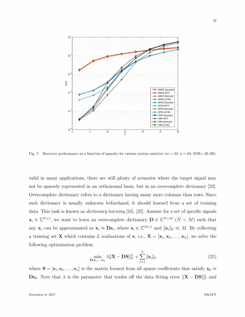
function of k and unrelated to n. Note, however, that if the measurement size is too small

and comparable to the sparsity (e.g., m < 2k in Fig. 7), performance of the sparse recovery

algorithms might not be appealing.

B. Predefined Basis or Learned Dictionary?

As discussed, to use CS techniques in wireless communication applications, we should

ensure that the target signal has a sparse representation. Traditional CS algorithm is per-

formed when the signal can be sparsely represented in an orthonormal basis, and many

robust recovery theories are based on this assumption [4]. Although such assumption is

11In fact, this is connected to many parameters such as dimension of vector and quality of system matrix.


22

0 5 10 15 20 25 3010

−5

10−4

10−3

10−2

10−1

100

MS

E

K

MMSE (Gaussian)MMSE (DFT)MMSE (Bernoulli)MMSE (LFSR)BPDN (Gaussian)BPDN (DFT)BPDN (Bernoulli)BPDN (LFSR)OMP (Gaussian)OMP (DFT)OMP (Bernoulli)OMP (LFSR)

Fig. 7. Recovery performance as a function of sparsity for various system matrices (m = 32, n = 64, SNR= 30 dB).

valid in many applications, there are still plenty of scenarios where the target signal may

not be sparsely represented in an orthonomal basis, but in an overcomplete dictionary [23].

Overcomplete dictionary refers to a dictionary having many more columns than rows. Since

such dictionary is usually unknown beforehand, it should learned from a set of training

data. This task is known as dictionary learning [24], [25]. Assume for a set of specific signals

xi ∈ CN×1, we want to learn an overcomplete dictionary D ∈ C

N×M (N < M) such that

any xi can be approximated as xi ≈ Dsi, where si ∈ CM×1 and ‖si‖0 ≪ M . By collecting

a training set X which contains L realizations of x, i.e., X = [x1,x2, . . . ,xL], we solve the

following optimization problem

minD,s1,...,sL

λ‖X − DS‖2F +

L∑

i=1

‖si‖0 (25)

where S = [s1, s2, . . . , sL] is the matrix formed from all sparse coefficients that satisfy xk ≈Dsk. Note that λ is the parameter that trades off the data fitting error ‖X − DS‖2

F and


23

sparsity of the representationL∑

i=1‖si‖0. Consider the measurement process y = Ax+n, where

A and n are the transfer function modeling the measurement process and the measurement

noise, respectively. Once the dictionary D is identified, we can express the system as y =

Hs + n where H = AD is the system matrix. After obtaining s from the CS technique, we

generate the estimated signal x = Ds. Notice that due to the non-orthogonality of D, new

theories are required to guarantee robust recovery [23], [26].

As an example to show the benefit of dictionary learning, we consider the downlink channel

estimation of the massive MIMO systems. When we employ the pilot-aided downlink channel

estimation, in which the basestation sends out pilots symbols A ∈ CT ×N during the training

period T and the user estimates the channel using the received vector y = Ah + n. In the

situation where the basestation has N antennas and the mobile user has a single antenna,

the channel vector is expressed as h ∈ CN×1. Traditional channel estimation schemes such as

least squares or MMSE estimation require more than or at least equal to N measurements

to estimate the channel reliably. In the massive MIMO regime where N is in the order of

hundred or more, this approach consumes too much downlink resources and impractical.

From our discussion, if h is sparse in some basis or dictionary D (i.e., h ≈ Ds, ‖s‖0 ≪ N),

then with the knowledge of A and D, s can be recovered from y = ADs + n using the

CS technique, and subsequently the channel h is estimated as h = Ds. Since the training

period proportional to the sparsity of s (T ∝ ‖s‖0) is enough when the CS technique is

used, training overhead can be reduced substantially. Since the downlink channel estimation

is feasible as long as ‖s‖0 is small, the key point here is whether we can find D such that

h can indeed be sparsely represented as h ≈ Ds.

A commonly used basis to induce sparsity is the orthogonal DFT basis which is derived

from a uniform linear array deployed at the basestation [12], [28], [36]. However, the spar-

sity assumption under the orthogonal DFT basis is valid only when the scatters in the

environment are extremely limited (e.g. a point scatter) and the number of antennas at

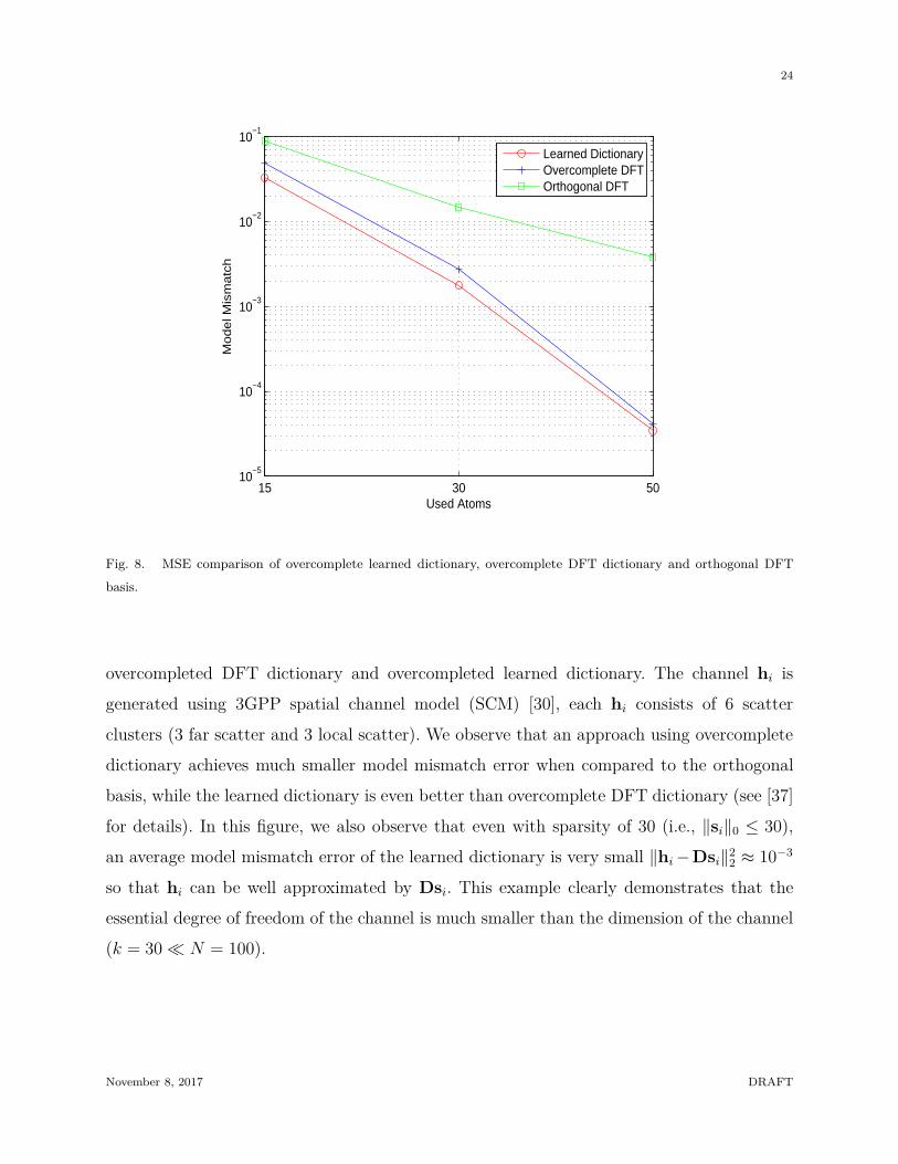
the basestation goes to infinity [29], which is not applicable in many cases. Fig. 8 depicts

the model mismatch error∑L

i=1 ‖hi − Dsi‖22/L as a function of the number of atoms in

D being used (i.e ‖si‖0). For each k (we test regarding to k = 15, 30, 50), we set the

constraint ‖si‖0 ≤ k for all i and then compare three types of D: orthogonal DFT basis,


24

15 30 5010

−5

10−4

10−3

10−2

10−1

Used Atoms

Mo

de

l Mis

ma

tch

Learned DictionaryOvercomplete DFTOrthogonal DFT

Fig. 8. MSE comparison of overcomplete learned dictionary, overcomplete DFT dictionary and orthogonal DFT

basis.

overcompleted DFT dictionary and overcompleted learned dictionary. The channel hi is

generated using 3GPP spatial channel model (SCM) [30], each hi consists of 6 scatter

clusters (3 far scatter and 3 local scatter). We observe that an approach using overcomplete

dictionary achieves much smaller model mismatch error when compared to the orthogonal

basis, while the learned dictionary is even better than overcomplete DFT dictionary (see [37]

for details). In this figure, we also observe that even with sparsity of 30 (i.e., ‖si‖0 ≤ 30),

an average model mismatch error of the learned dictionary is very small ‖hi −Dsi‖22 ≈ 10−3

so that hi can be well approximated by Dsi. This example clearly demonstrates that the

essential degree of freedom of the channel is much smaller than the dimension of the channel

(k = 30 ≪ N = 100).


25

C. What is the Desired Property for System Matrix?

A common misconception when using the CS techniques is that the signal can be recovered

accurately as long as the original signal vector is sparse. The condition that the desired

vector should be sparse is only necessary since the accurate recovery would not be possible

when a poorly designed system matrix is used. For example, suppose the support Ω of s is

Ω = 1, 3 and the first and third columns of H are exactly the same, then by no means the

recovery algorithm will work properly. This also motivates that the columns in H should

be designed to be as orthogonal to each other as possible. Intuitively, the more the system

matrix preserves the energy of the original signals, the better the quality of the recovered

signal would be. The system matrices supporting this idea need to be designed such that

each element of the measurement vector contains similar amount of information on the input

vector s. That is the place where the random matrix comes into play. Although an exact

quantification of the system matrix is complicated (see also next subsection), good news is

that most of random matrices, such as Gaussian (Hi,j ∼ N(0, 1m

)) or Bernoulli (Hi,j = ± 1m

),

well preserve the energy of the original sparse signal.

When the CS technique is applied to the wireless communications, the system matrix

H can be determined by the process of generating the transmit signal and/or wireless

channel characteristics. Fortunately, many of system matrices in wireless communication

systems behave like a random matrix. Similarly, the system matrix is modeled by a Bernoulli

random matrix when channel estimation is performed for code division multiplexing access

(CDMA) systems. Fading channel is often modeled as Gaussian random variables so that the

channel matrix whose columns correspond to the channel vectors between mobile terminal

and the basestation can be well modeled as a Gaussian random matrix. In Fig. 7, we plot the

performance of two well-known sparse recovery algorithms (BPDN and OMP) and MMSE

estimator for four distinct system matrices. In these results, we observe that the performance

using subsampled DFT and linear feedback shift register (LFSR)-based system matrix is not

much different from that using pure random matrices.

While the given system matrix in wireless applications is useful in many cases, in some

case we can also design the system matrix to improve the reconstruction quality. This task,

called sensing matrix design, is classified into two approaches. In the first approach, we


26

assume that the desired signal x is sparsely represented in a dictionary D. Then, the system

model is expressed as y = Hx = HDs. In this setup, the goal is to design H adapting to

dictionary D such that the columns in the combined equivalent dictionary E = HD has

good geometric properties [31]–[33]. In other words, we design H such that the columns in

E are as orthogonal to each other as possible. In the second type, rows of H are sequentially

designed using previously collected measurements as guidance [34], [35]. The basic idea is

to estimate the support from previous measurements and then allocate the sensing energy

to the estimated support element. Recently, the system design strategies to generate a nice

structure of system matrix in terms of recovery performance for massive MIMO systems

were proposed [17], [38].

D. What Recovery Algorithm Should We Use?

When the researchers consider the CS techniques in their applications, they can be

confused by a plethora of algorithms. There are hundreds of sparse recovery algorithms

in the literatures, and still many new ones are proposed each and every year. The tip

for not being flustered in a pile of algorithms is to clarify the main issues like the tar-

get specifications (performance requirements and complexity budget), system environments

(quality of system matrix, operating SNR regime), dimension of measurements and signal

vectors, and also availability of the extra information. Perhaps two most important issues

in the design of CS-based wireless communication systems are the mapping of the wireless

communication problem into the appropriate CS problem and the identification of the right

recovery algorithm. Often, one should modify the algorithm to meet the system require-

ments. Obviously, identifying the best algorithm for the target application is by no means

straightforward and one should have basic knowledge of the sparse recovery algorithm. In

this subsection, we provide a brief overview on four major approaches: ℓ1-norm minimization,

greedy algorithm, iterative algorithm, and statistical sparse recovery technique. Although not

all sparse recovery algorithms can be grouped into these categories, these four are important

in various standpoints such as popularity, effectiveness, and historical value.

• Convex optimization approach (ℓ1-norm minimization): As mentioned, with the

knowledge of the signal s being sparse, the most natural way to find a sparse input vector

under the system constraint (arg min ‖s‖0 s.t. y = Hs). Since the objective function


27

‖s‖0 is non-convex, solution of this problem can be found in a combinatoric way. As

an approach to overcome the computational bottleneck of ℓ0-norm minimization, ℓ1-

norm minimization has been used. If the noise power is bounded to ǫ, ℓ1-minimization

problem is expressed as

arg min ‖s‖1 s.t. ‖y − Hs‖2 < ǫ.

Basis pursuit de-noising (BPDN) [40], also called Lasso [44], relaxes the hard constraint

on the reconstruction error by introducing a soft weight λ as

s = arg mins

‖y − Hs‖2 + λ‖s‖1. (26)

The recovery performance of such ℓ1-minimization method can be further enhanced

by solving a sequence of weighted ℓ1 optimization [70]. Although the ℓ1-minimization

problem is convex optimization problem and thus efficient solvers exist, computational

complexity of this approach is still burdensome in implementing real-time wireless

communication systems.

• Greedy algorithm: In principle, the key mechanism of greedy algorithm is to suc-

cessively identify the subset of support (index set of nonzero entries) and refine them

until a good estimate of the support is found. Suppose the support is found accurately,

then the estimation of support elements would be straightforward since one can convert

the underdetermined system into overdetermined system by removing columns corre-

sponding to the zero element in s and then use a conventional estimation scheme like

MMSE or least squares (LS) estimator. In many cases, greedy algorithm attempts to

find the support in an iterative fashion, obtaining a sequence of estimates (s1, · · · , sn).

While the OMP algorithm picks an index of column of H one at a time using a

greedy strategy [45], recently proposed variants of OMP, such as generalized OMP

(gOMP) [48], compressive sampling matching pursuit (CoSaMP) [50], subspace pursuit

(SP) [51], and multipath matching pursuit (MMP) [79], have refined step to improve

the recovery performance. For example, gOMP select multiple promising columns in

each iteration. CoSaMp [50] and SP [51] incorporate special procedures to refine the

set of column indices by 1) choosing more than k columns of H, 2) recovering the

signal coefficients based on the projection onto the space of the selected columns,


28

and 3) rejecting those might not be in the true support. MMP performs the tree

search and then find the best candidate among multiple promising candidates obtained

from the tree search. In general, these approaches outperform the OMP algorithm

at the cost of higher computational complexity. In summary, the greedy algorithm

has computational advantage over the convex optimization approach while achieving

comparable (sometimes better) performance.

• Iterative algorithm: Sparse solution can be found by refining the estimate of sparse

signals in an iterative fashion. This approach includes iterative hard thresholding (IHT)

[52], [53] which iteratively performs the following update step

s(i+1) = T(

s(i) + HH(y − Hs(i))

, (27)

where s(i) is the estimate of the signal vector s at the ith iteration, which is initialized as

x(0) = 0. Algorithms similar to IHT yet exhibiting improved performance by exploiting

the message passing algorithm have also been proposed [71], [72].

• Statistical sparse recovery: Statistical sparse recovery algorithms treat the signal

vector s as a random vector and then infer it using the Bayesian framework. In the

maximum-a-posteriori (MAP) approach, for example, an estimate of s is expressed as

s = arg maxs

ln f(s|y) = arg maxs

ln f(y|s) + ln f(s),

where f(s) is the prior distribution of s. To model the sparsity nature of the signal

vector s, f(s) is designed in such a way that it decreases with the magnitude of s.

Well-known examples include i.i.d. Gaussian and Laplacian distribution. For example,

if i.i.d. Laplacian distribution is used, then the prior distribution f(s) is expressed as

f(s) =

(

λ

2

)N

exp

(

−λN∑

i=1

|si|)

.

Note that the MAP-based approach with the Laplacian prior model leads to the algo-

rithm similar to the BPDN in (26). When one chooses other super-Gaussian priors, the

model reduces to a regularized least squares problem [74]–[76], which can be solved by a

sequence of reweighted ℓ1 or ℓ2 algorithms. Different type of statistical sparse recovery

algorithms are sparse Bayesian learning (SBL) [78] and Bayesian compressed sensing

[54]. In these approaches, the priori distribution of the signal vector s is modeled as zero


29

TABLE I

Summary of sparse recovery algorithms

Approach Algorithm Features

Convex

optimization

BPDN [40] Reconstruction error ‖y − Hs‖2 regularized with ℓ1 norm

‖s‖1 is minimized. Convex optimization tools are needed.

Reweighted ℓ1

minimization

[70]

The BPDN can be improved via iterative reweighted ℓ1-

minimization. Computational complexity of this approach

is higher than the BPDN.

Greedy algorithm

OMP [45],

gOMP [48]

The indices of nonzero elements of s are identified in an

iterative fashion. Popular since it has low computational

complexity and also simple to implement.

CoSaMp [50],

SP [51]

More than K indices of the nonzero elements of s are found

and then candidates of poor quality are pruned afterwards.

These algorithm outperform OMP but they requires higher

complexity.

MMP [79] Tree search algorithm is adopted to search for the indices of

the nonzero elements in s efficiently. The algorithm offers

flexible means to control the trade-off between performance

and complexity.

Iterative algorithmIHT [52] Iterative thresholding step in (27) is performed repeatedly.

Implementation cost is low but the algorithm works well

under limited favorable scenarios.

AMP [72] Judicious approximations in message passing are used to

produce the algorithm with the improved performance over

IHT with comparable complexity.

Statistical sparse

recovery

MAP with

Laplacian prior

[73]

MAP estimation of the sparse vector is derived using Lapli-

cian distribution as sparsity-promoting prior distribution.

SBL [78], BCS

[54]

Hyper-parameter is used to model the variance of the

sparse signals. The EM algorithm is used to find the hyper-

parameter and signal vector iteratively.


30

mean Gaussian with the variance parameterized by a hyper-parameter. For example,

in SBL, it is assumed that each element of s is a zero mean Gaussian random variable

with variance γk (i.e., sk ∼ N (0, γk)). A suitable prior on the variance γk allows for

modeling of several super-Gaussian densities. Often a non-informative prior is used and

found to be effective. Let γ = γk, ∀k, then the hyperparameters Θ = γ, σ2 which

control the distribution of s and y can be estimated from data by marginalizing over s

and then performing evidence maximization or Type-II maximum-likelihood estimation

[77]:

Θ = arg maxΘ

p(y; γ, σ2)

= arg maxΘ

∫

p(y|s; σ2)p(s; γ)ds.(28)

The signal s can be inferred from the maximum-a-posterior (MAP) estimate after

obtaining Θ:

s = arg maxsp(s|y; Θ). (29)

By solving (28), we obtain the solution of γ with most of elements being zero. Note that

γ controls the variance of s, when γk = 0, it implies sk = 0, which results in a sparse

solution. It has been shown that with appropriately chosen parameters, SBL algorithm

is superior to ℓ1 and iteratively reweighted algorithms [78].

In Table I, we summarize the key features of the sparse recovery algorithms.

E. Can We Do Better If Multiple Measurement Vectors Are Available?

In many wireless communication applications, such as AoA and AoD estimation and

the channel estimation problem, multiple snapshots (more than one observation) are avail-

able and further the nonzero positions of these vectors are invariant or varying slowly.

The problem to recover the sparse vector from multiple observations, often called multiple

measurement vectors (MMV) problem, received much attention recently due to its supe-

rior performance compared to the single measurement vector (SMV) problem (see Fig. 9).

Group of measurements sharing common support are useful in many wireless communication

applications since multiple measurements filter out noise component and interference, and

also enhance the identification quality of the support. For example, when the MMV model

is considered in the sparse channel estimation, we can naturally exploit the property that


31

0 10 20 30 40 50 60 70 800

0.1

0.2

0.3

0.4

0.5

0.6

0.7

0.8

0.9

1

Sparsity

Exa

ct R

eco

ve

ry R

atio

OMPSOMP(L=2)SOMP(L=3)SOMP(L=4)

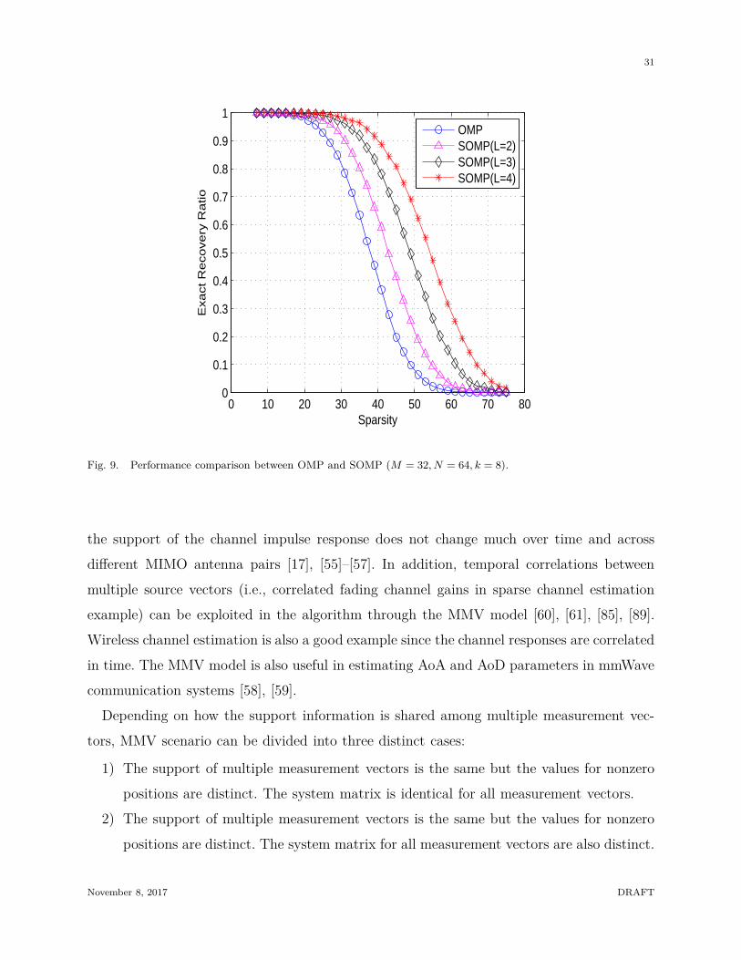
Fig. 9. Performance comparison between OMP and SOMP (M = 32, N = 64, k = 8).

the support of the channel impulse response does not change much over time and across

different MIMO antenna pairs [17], [55]–[57]. In addition, temporal correlations between

multiple source vectors (i.e., correlated fading channel gains in sparse channel estimation

example) can be exploited in the algorithm through the MMV model [60], [61], [85], [89].

Wireless channel estimation is also a good example since the channel responses are correlated

in time. The MMV model is also useful in estimating AoA and AoD parameters in mmWave

communication systems [58], [59].

Depending on how the support information is shared among multiple measurement vec-

tors, MMV scenario can be divided into three distinct cases:

1) The support of multiple measurement vectors is the same but the values for nonzero

positions are distinct. The system matrix is identical for all measurement vectors.

2) The support of multiple measurement vectors is the same but the values for nonzero

positions are distinct. The system matrix for all measurement vectors are also distinct.


32

TABLE II

Summary of MMV-based sparse recovery algorithms

Scenario References Remark

Scenario 1

SOMP [83] Extension of OMP for the MMV setup. Computational

complexity of the SOMP is lower than other candidate

algorithms.

Convex relaxation

[63]

Mixed ℓ1 norm is used to replace ℓ0 norm. The convex

optimization package is used for algorithm.

MSBL [62] Extention of SBL for the MMV setup. It offers excellent

recovery performance but the computational complexity is

a bit higher.

MUSIC-augmented

CS [66], [67]

The subspace criterion of MUSIC algorithm is used to

identify the support.

TSBL [85] Equivalence between block sparsity model and MMV model

was used to exploit the correlations between the source

vectors.

AR-SBL [60],

Kalman-filtered CS

[68]

The multiple source vectors are modeled by auto-regressive

process. The support and amplitude of the source vectors

is jointly estimated via iterative algorithm.

Scenario 2

KSBL [61] The auto-regressive process is used to model the dynamics

of the source vectors. Kalman filter is incorporated to

estimate the support and gains sequentially.

AMP-MMV [90] Graphical model is used to describe the variations of the

source vectors. Message passing over a part of graph having

dense connections is handled via the AMP method [71].

sKTS [89] The deterministic binary vector is used to model the spar-

sity structure of the source vectors. The EM algorithm is

used for joint estimation of sparsity pattern and gains.

Scenario 3Modified-CS [92] The new elements added to the support detected in the pre-

vious measurement vector is found via ℓ1 optimization. The

candidates of poor quality are eliminated via thresholding.

DCS-AMP [91] The dynamic change of the support is modeled by the

markov process and efficient message passing algorithm

based on AMP is applied.


33

3) The support of multiple measurement vectors slightly changes.

The first scenario is the conventional expression of the MMV problem. In this scenario, we

express the measurement vectors as

Y = HS + N (30)

where Y = [y1 · · · yN ], S = [s1 · · · sN ], and N = [n1 · · · nN ]. The recovery algorithm

finds the column indices of H corresponding to the nonzero row vectors of S using the

measurement matrix Y. By exploiting the common support information in MMV scenario,

performance of the recovery algorithm can be improved substantially over the SMV-based

recovery algorithm [81]–[84]. Various recovery algorithms have been proposed for MMV

scenario. In [63], the convex relaxation method based on mixed norm has been proposed. In

[83], the greedy algorithm called simultaneous OMP (SOMP) is proposed. From theoretic

analysis, it has been shown that the performance of the MMV-based algorithm improves

exponentially with the number of measurements [64], [65]. Statistical sparse estimation

techniques for MMV scenario include MSBL [84], AR-SBL [60], and TSBL [85]. In [66], [67],

an approach to identify the direction of arrival (DoA) in array signal processing using the

MMV model has been investigated. Using the close connection between the DoA estimation

problem and the MMV model, the recovery algorithms are devised such that the subspace

criterion of the MUSIC algorithm is augmented with the CS recovery algorithm. Further

improvement in the recovery performance can be achieved by exploiting the statistical

correlations between the signal amplitudes [60], [68], [85].

The second scenario is slightly more general in the sense that system matrices are different

for all measurement vectors. Extensions of OMP algorithm [86], iteratively reweighted algo-

rithm [87], sparse Bayesian learning algorithm [87], [88], and Kalman-based sparse recovery

algorithm [89] can be applied to this setting. In [90], it has been shown that the graph-based

inference method is effective in this scenario. In the last scenario, the recovery algorithms

need to keep track of temporal variations of the signal support since the sparsity pattern

changes slowly in time. However, since the variation is small, the sparsity pattern can be

tracked by estimating the difference between two support sets for consecutive measurement

vectors [92], [93]. The algorithm employing approximate message passing (AMP) is provided

for this scenario in [91]. In Table II, we summarize the recovery algorithms based on the


34

24 26 28 30 32 34 36 3810

−4

10−3

10−2

10−1

SNR (dB)

SE

R

Oracle MMSE

MMSE

OMP

OMPslice

CoSaMP

MMP

sMMP

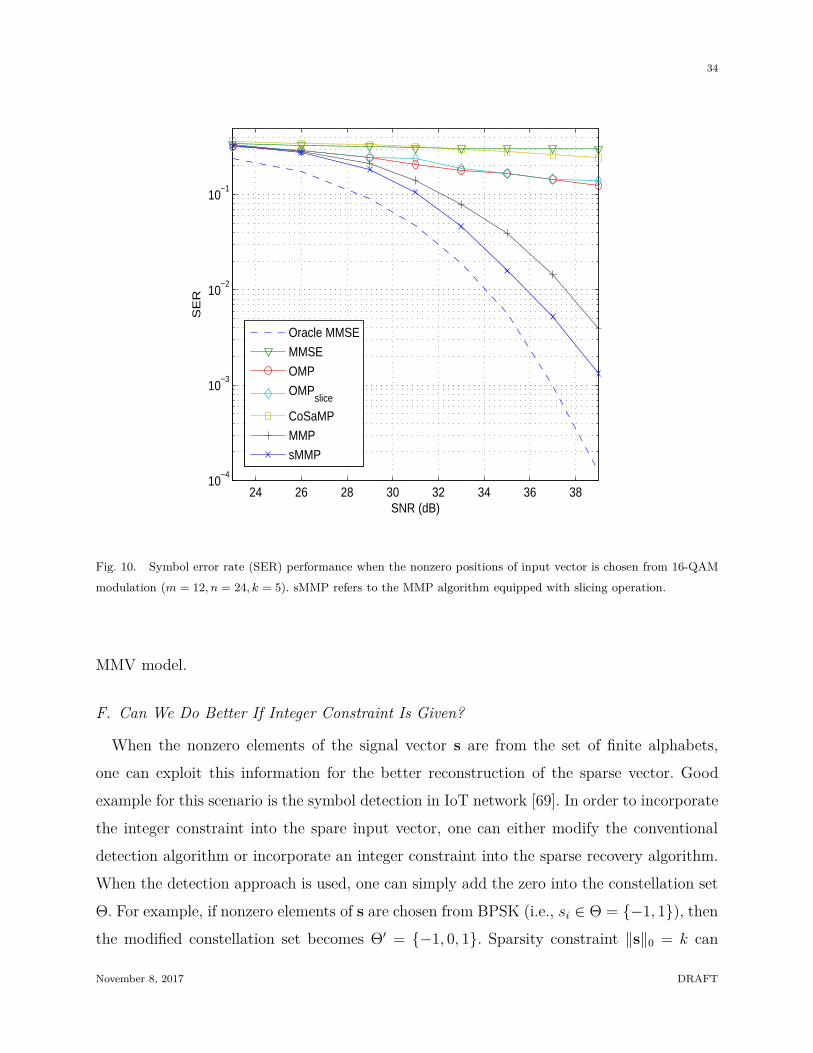
Fig. 10. Symbol error rate (SER) performance when the nonzero positions of input vector is chosen from 16-QAM

modulation (m = 12, n = 24, k = 5). sMMP refers to the MMP algorithm equipped with slicing operation.

MMV model.

F. Can We Do Better If Integer Constraint Is Given?

When the nonzero elements of the signal vector s are from the set of finite alphabets,

one can exploit this information for the better reconstruction of the sparse vector. Good

example for this scenario is the symbol detection in IoT network [69]. In order to incorporate

the integer constraint into the spare input vector, one can either modify the conventional

detection algorithm or incorporate an integer constraint into the sparse recovery algorithm.

When the detection approach is used, one can simply add the zero into the constellation set

Θ. For example, if nonzero elements of s are chosen from BPSK (i.e., si ∈ Θ = −1, 1), then

the modified constellation set becomes Θ′ = −1, 0, 1. Sparsity constraint ‖s‖0 = k can


35

also be used to limit the search space of the detection algorithm. On the other hand, when

the sparse recovery algorithm is used, one should incorporate the quantization step to map

real (complex) value into the symbol. In other words, whenever the estimate si is generated,

we use the quantized output QΩ(si). Note, however, that just using the quantized output

might not be effective, in particular for the sequential greedy algorithms due to the error

propagation. For example, if an index is chosen incorrectly in one iteration, then the estimate

will also be incorrect and thus the quantized output will bring additional quantization error,

deteriorating the subsequent detection process. In this case, parallel tree search strategy can

be a good option to recover the discrete sparse vector. For example, a tree search algorithm

(e.g., MMP) performs the parallel search to find multiple promising candidates [79]. Among

the multiple candidates, the best one minimizing the residual magnitude is chosen in the

last minute. The main benefit of tree search method, in the perspective of incorporating

the integer slicer, is that it deteriorates the quality of incorrect candidate yet enhances the

quality of correct one. This is because the quality of incorrect candidates gets worse due to

the additional quantization noise caused by the slicing while no such phenomenon happens

to be the correct one (recall that the quantization error is zero for the correct symbol). As

a result, as shown in Fig. 10, the recovery algorithms accounting for the integer constraint

of the symbol vector outperform those without considering this property.

G. Should We Know Sparsity a priori?

Some algorithm requires the sparsity of an input signal while others do not need this. For

example, sparsity information is unnecessary for the ℓ1-norm minimization approaches but

many greedy algorithms need this since the sparsity equals the number of iterations. When

needed, one should estimate the sparsity using various heuristics. Before we discuss on this,

we need to consider what will happen when an incorrect sparsity is used. In a nutshell,

setting the number of iteration not being equivalent to the sparsity leads to either early

or late termination of the greedy algorithm. In the former case (i.e., underfitting scenario),

the desired signal will not be fully recovered while some of the noise vector is treated as a

desired signal for the latter case (i.e., overfitting scenario). Both cases are undesirable, but

performance loss is typically more severe for underfitting due to the loss of the signal so

that it might be safe to use slightly higher sparsity. For example, if the sparsity estimate is


36

k, one can take 1.2k as an iteration number of OMP.

As a sparsity estimation strategy, residual-based stopping criterion and cross validation

[80] are popular. The residual based stopping criterion is widely used to identify the sparsity

level (or iteration number) of the greedy algorithm. Basically, this scheme terminates the

algorithm when the residual power is smaller than the pre-specified threshold ǫ (i.e., ‖ri‖2 <

ǫ). The iteration number at the termination point is set to the sparsity level. However,

since the residual magnitude decreases monotonically and the rate of decay depends on

the system parameters, it might not be easy to identify the optimal terminating point.

Cross validation (CV) is another technique to identify the model order (sparsity level k

in this case) [80]. In this scheme, the measurement vector y are divided into two parts: a

training vector y(t) and a validation vector y(v). In the first step, we generate a sequence of

possible estimates s1, · · · , sn using a training vector y(t), where si denotes the estimate of s

obtained under the assumption that the sparsity equals i. In the second step, the sparsity

is predicted using the validation vector y(v). Specifically, for each estimate si, the validation

error ǫi = ‖y(v) − H(v)si‖2 is computed. Initially, when the count i increases, the quality

of the estimate improves and thus the validation error ǫi will decrease. However, when the

count i exceeds the sparsity, that is, when we choose more columns than needed, we observe

no more decrease in ǫi and noise will be added to the validation error. In view of this,

the number generating the minimum validation error is returned as the sparsity estimate

(k = arg mini ǫi).

V. Conclusion

In this article, we provide an overview of compressed sensing (CS) technique for wireless

communication systems. We discussed basics of CS techniques, four subproblems related

to wireless communication systems, and wireless applications which CS techniques can be

applied to. We also discussed several main issues that one should be aware of and subtle

points that one should pay attention to. There are a broad class of wireless applications

to which the CS technique would be beneficial and much work remains to improve the

performance of future wireless communication systems. We list here some of future research

directions.


37

• It would be interesting to design an adaptive sparse recovery algorithm that performs

well in various and diverse wireless environments and input conditions.

• Most of performance metrics in wireless communication system are statistical (e.g.,

BER, BLER) and it would be useful to have more realistic analysis tool based on

statistical approach.

• It might be worth investigating if the machine learning technique would be helpful in

designing the system matrix (e.g., precoder, codebook) for massive multiuser systems.

Note that it is very difficult to find out the optimal precoding strategy (e.g., dirty paper

coding) for massive multiuser communication systems and machine learning approach

such as deep neural network might provide an answer to the problem.

• What if the system matrix is sparse, not the input vector. In this work, we have

primarily discussed the scenario where the desired input vector is sparse. But there

is some scenario where the input-output connection is sparse, not the input vector

(e.g., massive multiple access scheme).

• We did not have thorough discussion on the implementation issue in this work. For the

successful development of CS technique for wireless communication systems, fast real-

time implementation is of great importance. Development of implementation friendly

algorithm and architecture would expedite the commercialization of CS-based wireless

systems.

As a final remark, we hope that this article will serve as a useful guide for wireless

communication researchers, in particular for those who are interested in CS, to grasp the

gist of this interesting paradigm. Since our treatment in this paper is rather casual and

non-analytical, one should dig into details with further study. However, if the readers learn

in mind that essential knowledge in a pile of information is always sparse, the journey will

not be that tough.

Acknowledgment

The authors would like to thank the anonymous reviewers for their invaluable comments

and suggestions, which helped us to improve the quality of the paper.


38

VI. Proof of Theorem 1

We first consider only if case. We assume that there are more than one vector, say s1 and

s2, satisfying y = Hs and both have at most k nonzero elements. Then, by letting u = s1−s2,

we have Hu = 0 where u has at most 2k nonzero elements. Since spark(H) > 2k from the

hypothesis, any 2k columns in H are linearly independent, implying that u = 0 and hence

s1 = s2. We next consider the if case. We assume that, for given y, there exists at most

one k-sparse signal s satisfying y = Hs and spark(H) ≤ 2k. Under this hypothesis, there

exists a set of 2k columns that are linearly dependent, implying that there exists 2k-sparse

vector u in N(H) (i.e., Hu = 0). Since u is 2k-sparse, we can express it into the difference

of two k-sparse vectors s1 and s2 (u = s1 − s2). Since Hu = 0, H(s1 − s2) = 0 and hence

Hs1 = Hs2, which contradicts the hypothesis that there is at most one k-sparse solution

satisfying y = Hs. Thus, we should have spark(H) > 2k.

References

[1] D. Donoho, “Compressed sensing,” IEEE Trans. Inform. Theory, vol. 52, no. 4, pp. 1289-1306, April 2006.

[2] A. V. Oppenheim and R. W. Schafer, Discrete-time Signal Processing, Prentice Hall, 2010.

[3] R. G. Baraniuk, “Compressive sensing,” IEEE Signal Processing Mag., vol. 24, pp. 118-121, July 2007.

[4] E. J. Candes and M. B. Wakin, “An introduction to compressive sampling,” IEEE Signal Processing Mag., vol.

25, pp. 21-30, March 2008.

[5] Y. C. Eldar and G. Kutyniok, Compressed Sensing : Theory and Applications, Cambridge Univ. Press, 2012.

[6] Z. Han, H. Li, and W. Yin, Compressive Sensing for Wireless Networks, Cambridge Univ. Press, 2013.

[7] S. Foucart and H. Rauhut, A Mathematical Introduction to Compressive Sensing, Applied and Numerical Harmonic

Analysis, Birkhauser, 2013.

[8] M. Fornasier and H. Rauhut. Compressive sensing, In Handbook of Mathematical Methods in Imaging, pp 187-

228. Springer, 2011.

[9] K. Hayashi, M. Nagahara, and T. Tanaka, “A user’s guide to compressed sensing for communications systems,”

IEICE Trans. Commun., vol. E96-B, no. 3, pp. 685-712, March 2013.

[10] C. R. Berger, S. Zhou, J. C. Preisig and P. Willett, “Sparse channel estimation for multicarrier underwater

acoustic communication: from subspace methods to compressed sensing,” IEEE Trans. Signal Process., vol. 58,

pp. 1708-1721, March 2010.

[11] W. Li and J. C. Preisig, “Estimation of rapidly time-varying sparse channels,” IEEE J. Oceanic Eng., vol. 32,

pp. 927-939, Oct. 2007.

[12] W. U. Bajwa, J. Haupt, A. M. Sayeed, and R. Nowak, “Compressed channel sensing: A new approach to

estimating sparse multipath channels,” Proceedings of the IEEE, vol. 98, no. 6, pp. 1058-1076, June 2010.

[13] S. F. Cotter and B. D. Rao, “Sparse channel estimation via matching pursuit with application to equalization,”

IEEE Trans. Commun., vol. 50, no. 3, pp. 374-377, March 2002.


39

[14] R. Prasad, C. R. Murthy, and B. D. Rao, “Joint Approximately Sparse Channel Estimation and Data Detection

in OFDM Systems Using Sparse Bayesian Learning,” IEEE Trans. Signal Process., vol 62, no. 14, pp. 3591-3603,

July 2015.

[15] 3GPP TS 36.101. “User Equipment (UE) Radio Transmission and Reception.” 3rd Generation Partnership

Project; Technical Specification Group Radio Access Network (E-UTRA). URL: http://www.3gpp.org.

[16] M. Masood, L. H. Afify, and T. Y. Al-Naffouri, “Efficient coordinated recovery of sparse channels in massive

MIMO,” IEEE Trans. Signal Process., vol. 63, no. 1, pp. 104-118, Jan. 2015.

[17] J. W. Choi, B. Shim, and S. Chang, “Downlink Pilot Reduction for Massive MIMO Systems via Compressed

Sensing,” IEEE Commun. Letter, vol. 19, no. 11, pp. 1889-1892, Nov. 2015.

[18] T. Al-Naffouri, A. Quadeer, F. Al-Shaalan, H. Hmida, “Impulsive noise estimation and cancellation in DSL using

compressive sampling,” Proc. IEEE International Symp. Circuits and Systems (ISCAS), May 2011, pp. 2133-2136.

[19] T. K. Moon and W. Stirling, Mathematical Methods And Algorithms For Signal Processing, Prentice Hall, 1999.

[20] L. Atzori, A. Lera, G. Morabito, “The Internet of Things: A survey,” Computer Networks, vol. 54, no. 11, pp.

2787-2805, Oct. 2010.

[21] D. Cohen and Y. C. Eldar, “Sub-Nyquist sampling for power spectrum sensing in cognitive radios: a unified

approach,” IEEE Trans. Signal Process., vol. 62, no. 15, pp. 3897-3910, August 2014.

[22] J. W. Choi and B. Shim, “New approach for massive MIMO detection using sparse error recovery,” Proc. of

IEEE GLOBECOM conf. 2014.

[23] E. J. Candes, Y. C. Eldar, D. Needell, and P. Randall, “Compressed sensing with coherent and redundant

dictionaries,” Applied and Comp. Harmonic Anal., vol. 31, no. 1, pp. 59-73, July 2011.

[24] K. Kreutz-Delgado, J. F. Murray, B. D. Rao, K. Engan, T. Lee, and T. J. Sejnowski, “Dictionary learning

algorithms for sparse representation,” Neural Computation, vol. 15, no. 2, pp. 349-396, Feb. 2003.

[25] M. Aharon, M. Elad, and A. Bruckstein, “K-SVD: An algorithm for designing overcomplete dictionaries for

sparse representation,” IEEE Trans. Signal Process., vol. 54, no. 11, pp. 4311-4322, Nov. 2006.

[26] H. Rauhut, K. Schnass, and P. Vandergheynst, “Compressed sensing and redundant dictionaries,” IEEE Trans.

Inf. Theory, vol. 54, no. 5, pp. 2210-2219, May 2008.

[27] C. R. Berger and W. Zhaohui, H. Jianzhong, and Z. Shengli, “Application of compressive sensing to sparse

channel estimation,” IEEE Commun. Magazine, vol. 48, no. 11, pp. 164-174, Nov. 2010.

[28] X. Rao and V. K. N. Lau, “Distributed compressive CSIT estimation and feedback for FDD multi-user massive

MIMO systems,” IEEE Trans. Signal Process., vol. 62, no. 12, pp. 3261-3271, June 2014.

[29] A. M. Sayeed, “Deconstructing multiantenna fading channels,” IEEE Trans. Signal Process., vol. 50, no. 10, pp.

2563-2579, Oct. 2002.

[30] 3GPP TS 25.996. “Universal Mobil Telecommunications System (UMTS); Spatial channel model for Multiple

Input Multiple Output (MIMO) simulations,” version 12.0.0 Release 12, Sep 2014. URL: http://www.3gpp.org.

[31] M.Elad, “Optimized projections for compressed sensing,” IEEE Trans. Signal Process., vol. 55, no. 12, pp. 5695-

5702, 2007.

[32] J.M.Duarte-Carvajalino and G.Sapiro, “Learning to sense sparse signals: Simultaneous sensing matirx and

sparsifying dictionary optimization,” IEEE Trans. Image Process., vol .18, no. 7, pp. 1395-1408, 2009.

[33] Y.Yu, A.P.Petropulu, and H.V.Poor, “Measurement matrix design for compressive sensing-based mimo radar,”

IEEE Trans. Signal Process., vol. 59, no. 11, pp. 5338-5352, 2011.


http://www.3gpp.org

http://www.3gpp.org

40

[34] M.L.Malloy and R.D.Nowak, “Near-optimal adaptive compressed sensing,” Information Theory, IEEE Transac-

tions on, vol. 60, no. 7, pp. 4001-4012, 2014.

[35] J.Haupt, R. Baraniuk, R.Castro, and R.Nowak, “Sequentially designed compressed sensing,” in Statistical Signal

Processing Workshop (SSP), 2012, pp.401-404.

[36] O. E. Ayach, S. Rajagopal, S. Abu-Surra, and P. Zhouyue, and R. W. Heath, “Spatially sparse precoding in

millimeter wave MIMO systems,” IEEE Trans. Wireless Commun., vol. 13, no. 3, pp. 1499-1513, March 2014.

[37] Y. Ding and B. D. Rao, “Channel estimation using joint dictionary learning in fdd massive mimo systems,” in

2015 IEEE Global Conference on Signal and Information Processing (GlobalSIP). IEEE, 2015, pp. 185-189,

[38] C. Qi and W. Wu, “A study of deterministic pilot allocation for sparse channel estimation in OFDM systems,”

IEEE Commun. Letter, vol. 16, no. 5, pp. 742-744, May 2012.

[39] E. Candes, J. Romberg, and T. Tao, “Stable signal recovery from incomplete and inaccurate measurements,”

Comm. Pure Appl. Math., vol. 59, no. 8, pp. 1207-1223, Aug. 2006.

[40] S. S. Chen, D. L. Donoho, and M. A. Saunders, “Atomic decomposition by basis pursuit,” SIAM J. Scientif.

Comput., vol. 20, no. 1, pp. 33-61, 1998.

[41] http://cvxr.com/cvx/

[42] http://users.ece.gatech.edu/justin/l1magic/

[43] S. J. Kim, K. Koh, M. Lustig, S. Boyd, and D. Gorinevsky, “An interior-point method for large-scale ℓ1-

regularized least squares,” IEEE Journal on Sel. Topics in Signal Process. vol. 1, pp. 606-617, Dec. 2007.

[44] R. Tibshirani, “Regression shrinkage and selection via the lasso,” Journal of the Royal Statistical Society, Series

B, vol. 58, no. 1, pp. 267-288, 1996.

[45] J. A. Tropp and A. C. Gilbert, “Signal recovery from random measurements via orthogonal matching pursuit,”

IEEE Trans. Inform. Theory, vol. 53, no. 12, pp. 4655-4666, Dec. 2007.

[46] T. Strohmer and R. Heath, “Grassmannian frames with applications to coding and communication measure-

ments,” Appl. Comput. Harmon. Anal., vol. 53, vol. 14, pp. 257-275, 2004.

[47] D. Donoho and M. Elad, “Optimally sparse representation in general (non-orthogonal) dictionaries via L1

minimization,” Proc. Natl. Acad. Sci., vol. 100, pp. 2197-2202, 2003.

[48] J. Wang, S. Kwon, and B. Shim, “Generalized orthogonal matching pursuit,” IEEE Trans. Signal Process., vol.

60, no. 12, pp. 6202-6216, Dec. 2012.

[49] T. Zhang, “Sparse recovery with orthogonal matching pursuit under rip,” IEEE Trans. Inform. Theory, vol. 57,

no. 9, pp. 6215.6221, Sept. 2011.

[50] D. Needell and J. A. Tropp, “CoSaMP: iterative signal recovery from incomplete and inaccurate samples,” Appl.

Comput. Harmon. Anal., vol. 26, pp. 301-321, 2009.

[51] W. Dai and O. Milenkovic, “Subspace pursuit for compressive sensing signal reconstruction,” IEEE Trans.

Information Theory, vol. 55, pp. 2230-2249, May 2009.

[52] T. Blumensath and M. E. Davies, “Iterative hard thresholding for compressed sensing,” Appl. Comput. Harmon.

Anal., vol. 27, no. 3, pp. 265-274, 2009.

[53] A. Maleki and D. L. Donoho, “Optimally tuned iterative reconstruction algorithms for compressed sensing,”

IEEE Journal of Selected Topics in Signal Process., vol. 4, no. 2, pp, 330-341, April 2010

[54] S. Ji, Y. Xue, and L. Carin, “Bayesian compressed sensing,” IEEE Trans. Signal Process., vol. 56, pp. 2346-2356,

June 2008.


http://cvxr.com/cvx/

http://users.ece.gatech.edu/justin/l1magic/

41

[55] Z. Gao, L. Dai, W. Dai, B. Shim, and Z. Wang, “Structured compressive sensing-based spatio-temporal joint

channel estimation for FDD massive MIMO,” IEEE Trans. Commun., vol. 64, no. 2, pp. 601-617, Feb. 2016.

[56] Y. Barbotin, A. Hormati, S. Rangan, and M. Vetterli, “Estimation of sparse MIMO channels with common

support,” IEEE Trans. Commun., vol. 60, no. 12, pp. 3705-3716, Dec. 2012.

[57] X. Rao, and V. K. N. Lau, “Distributed compressive CSIT estimation and feedback for FDD multi-user massive

MIMO systems,” IEEE Trans, Signal Process., vol. 62, no. 12, pp. 3261-3271, Jun. 2014.

[58] A. Alkhateeb, O. E. Ayach, G. Leus, and R. W. Heath, “Channel estimation and hybrid precoding for millimeter

wave cellular systems,” IEEE J. Sel. Topics Signal Process., vol. 8, pp. 831-846, Oct. 2014.

[59] Y. Y. Lee, C. Wang, and Y. H. Huang, “A Hybrid RF/Baseband precoding processor based on parallel-index-

selection matrix-inversion-bypass simultaneous orthogonal matching pursuit for millimeter wave MIMO systems,”

IEEE Trans. Signal Process., vol. 63, no. 2, pp. 305-317, Jan. 2015.

[60] Z. Zhang and B. D. Rao, “Sparse signal recovery in the presence of correlated multiple measurement vectors,”

Proc. ICASSP 2010, Dallas, TX USA, 2010, pp. 3986-3989.

[61] R. Prasad, C. R. Murphy and B. D. Rao, “Joint approximately sparse channel estimation and data detection

in OFDM systems using sparse Bayesian learning,” IEEE Trans. Signal Process., vol. 62, no. 14, pp. 3591-3603,

July 2014.

[62] S. F. Cotter, B. D. Rao, K. Engan, K. Kreutz-Delgado, “Sparse solutions to linear inverse problems with multiple

measurement vectors,” IEEE Trans. Signal Process., vol. 53, pp. 2477-2488, July 2005.

[63] J. A. Tropp, A. C. Gilbert, M. J. Strauss, “Algorithms for simultaneous sparse approximation. Part II: convex

relaxation,” Signal Processing, vol. 86, pp. 589-602, 2006.

[64] Y. C. Eldar and H. Rauhut, “Average case analysis of multichannel sparse recovery using convex relaxation,”

IEEE Trans. Information Theory, vol. 56, no. 1, pp. 505-519, Jan. 2010.

[65] R. Gribonval, H. Rauhut, K. Schnass, and P. Vandergheynst, “Atoms of all channels, unite! Average case analysis

of multi-channel sparse recovery using greedy algorithms,” J. Fourier Anal. Appl., vol. 14, no. 5, pp. 655-687,

2008.

[66] J. Kim, O. Lee, and J. Ye, “Compressive MUSIC: revisiting the link between compressive sensing and array

signal processing,” IEEE Trans. Inf. Theory, vol. 58, no. 1, pp. 278-301, 2012.

[67] K. Lee, Y. Bresler, and M. Junge, “Subspace methods for joint sparse recovery,” IEEE Trans. Inf. Theory, vol.

58, no. 6, pp. 3613-3641, 2012.

[68] N. Vaswani, “Kalman filtered compressed sensing,” Proc. ICIP San Diego, CA USA, 2008, pp. 893-896.

[69] H. Zhu and G. B. Giannakis, “Exploiting sparse user activity in multiuser detection,” IEEE Trans. Commun.,

vol. 59, no. 2, pp. 454-465, Feb. 2011.

[70] E. Candes, M. Wakin, and S. Boyd, “Enhancing sparsity by reweighted ℓ1 minimization,” J. Fourier Anal. Appl.,

vol. 14, pp. 877-905, 2008

[71] D. L. Donoho, A. Maleki, and A. Montanari, “Message passing algorithms for compressed sensing,” Proc. of the

National Academy of Sciences, vol. 106, pp. 18914-18919, Nov. 2009.

[72] M. Bayati and A. Montanari, “The dynamics of message passing on dense graphs, with applications to compressed

sensing,” IEEE Trans. Inform. Theory, vol. 57, pp. 764-785, Feb. 2011.

[73] M. Figueiredo, “Adaptive sparseness using Jeffreys prior,” Advances in Neural Information Processing Systems

(NIPS), 2002.


42

[74] I. F. Gorodnitsky and B. D. Rao, “Sparse signal reconstruction from limited data using FOCUSS: A re-weighted

minimum norm algorithm,” IEEE Trans. Signal Process., vol. 45, no. 3, pp. 600-616, March 1997.

[75] E. J. Candes, M. B. Wakin, and S. P. Boyd, “Enhancing sparsity by reweighted ℓ1 minimization,” Fourier anal.

and appl. vol. 14, no. 5-6, pp. 877-905, Dec. 2008.

[76] R. Chartrand and W. Yin, “Iteratively reweighted algorithms for compressive sensing,” IEEE Proc. ICASSP

2008, pp. 3869-3872, March 2008.

[77] M. E. Tipping, “Sparse Bayesian learning and the relevance vector machine,” The journal of machine learning

research, vol. 1, pp. 211-244, 2001.

[78] D. P. Wipf and B. D. Rao, “Sparse Bayesian learning for basis selection,” IEEE Trans. Signal Process., vol. 52,

no. 8, pp. 2153-2164, August 2004.

[79] S. Kwon, J. Wang, and B. Shim, “Multipath matching pursuit,” IEEE Trans. Inf. Theory, vol. 60, no. 5, pp.

2986-3001, May 2014.

[80] R. Ward, “Compressed sensing with cross validation,” IEEE Trans. Inf. Theory, vol. 55, no. 12, pp. 5773-5782,

Dec. 2009.

[81] Y. C. Eldar and H. Rauhut, “Average case analysis of multichannel sparse recovery using convex relaxation,”

IEEE Trans. Inf. Theory, vol. 6, no. 1, pp. 505-519, Jan. 2010.

[82] S. F. Cotter, B. D. Rao, K. Engan, and K. Kreutz-Delgado, “Sparse solutions to linear inverse problems with

multiple measurement vectors,” IEEE Trans. Signal Process. vol. 53, no. 7, pp. 2477-2488, July 2005.

[83] J. A. Tropp, A. C. Gilbert, and M. J. Strauss, “Algorithms for simultaneous sparse approximation. Part I: greedy

pursuit,” Signal Process., vol. 86, no. 3, pp. 572-588, March 2006.

[84] D. P. Wipf and B. D. Rao, “An empirical Bayesian strategy for solving the simultaneous sparse approximation

problem,” IEEE Trans. Signal Process. vol. 55, no. 7, pp. 3704-3716, July 2007.

[85] Z. Zhang and B. D. Rao, “Sparse signal recovery with temporally correlated source vectors using sparse Bayesian

learning,” IEEE Journal of Selected Topics in Signal Processing, vol. 5, pp. 912-926, Sept. 2011.

[86] M. F. Duarte, S. Sarvotham, and D. Baron, M. B. Wakin, and R. G. Baraniuk, “Distributed compressed sensing

of jointly sparse signals,” Proc. Asilomar Conf. Signals, Sys. Comput., pp. 1537-1541, May 2005.

[87] Y. Ding and B. D. Rao, “Joint dictionary learning and recovery algorithms in a jointly sparse framework,” in

2015 49th Asilomar Conference on Signals, Systerms and Computers. IEEE, 2015, pp. 1482-1486.

[88] S. Ji, D. Dunson, and L. Carin, “Multitask compressive sensing,” IEEE Trans. Signal Process., vol. 57, no. 1,

pp. 92-106, Jan. 2009.

[89] J. W. Choi and B. Shim, “Statistical Recovery of Simultaneously Sparse Time-Varying Signals From Multiple

Measurement Vectors,” IEEE Trans. Signal Process., vol. 63, no. 22, pp. 6136-6148, Nov. 2015.

[90] J. Ziniel and P. Schniter, “Efficient high-dimensional inference in the multiple measurement vector problem,”

IEEE Trans. Signal Process., vol. 61, pp. 340-354, Jan. 2013.

[91] J. Ziniel and P. Schniter, “Dynamic compressive sensing of time-varying signals via approximate message

passing,” IEEE Trans. Signal Process., vol. 61, no. 21, pp. 5270-5284, Nov. 2015.

[92] N. Vaswani and W. Lu, “Modified-CS: modifying compressive sensing for problems with partially known

support,” IEEE Trans. Signal Process., vol. 58, no. 9, pp. 4595-4607, Sept. 2010.

[93] X. Rao and V. K. N. Lau, “Compressive sensing with prior support quality information and application to


43

massive MIMO channel estimation with temporal correlation,” IEEE Trans. Signal Process., vol. 63, no. 18, pp.

4914-4924, Sept. 2015.


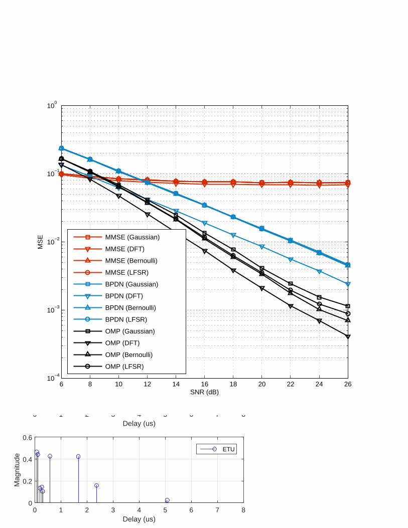
Delay (us)0 1 2 3 4 5 6 7 8

Mag

nitu

de

0

0.2

0.4

0.6

0.8

EVA

Delay (us)0 1 2 3 4 5 6 7 8

Mag

nitu

de

0

0.2

0.4

0.6

ETU

6 8 10 12 14 16 18 20 22 24 2610

−4

10−3

10−2

10−1

100

MS

E

SNR (dB)

MMSE (Gaussian)

MMSE (DFT)

MMSE (Bernoulli)

MMSE (LFSR)

BPDN (Gaussian)

BPDN (DFT)

BPDN (Bernoulli)

BPDN (LFSR)

OMP (Gaussian)

OMP (DFT)

OMP (Bernoulli)

OMP (LFSR)

0 0 0 0 0 0 0 0 0 0 0 0 0 0 0 0 0

0 0 0 0 0 0 0 0 0 0 0 0 0 0 0 0 0

0 0 0 0 0 0 0 0 0 0 0 0 0 0 0 0 0

0 0 0

0 0 0

0 0 0

0 0 0

0 0 0 0 0 0 0 0 0 0 0 0

0 0 0 0 0 0 0 0 0 0 0 0

0 0 0 0 0 0 0 0 0 0 0 0

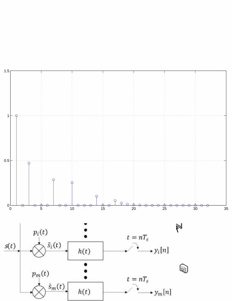
0 5 10 15 20 25 30 350

0.5

1

1.5

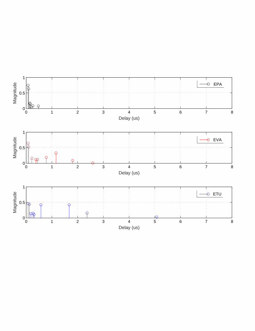
0 1 2 3 4 5 6 7 80

0.5

1

Delay (us)

Mag

nitu

de

EPA

0 1 2 3 4 5 6 7 80

0.5

1

Delay (us)

Mag

nitu

de

EVA

0 1 2 3 4 5 6 7 80

0.5

1

Delay (us)

Mag

nitu

de

ETU

Documents

Compressed Sensing for Wireless Communications : Useful ... · Compressed Sensing for Wireless Communications : Useful Tips and Tricks ... it is not easy to come up with simple and