Lecture: Algorithms for Compressed Sensing

Zaiwen Wen

Beijing International Center For Mathematical ResearchPeking University

http://bicmr.pku.edu.cn/~wenzw/bigdata2018.htmlwenzw@pku.edu.cn

Acknowledgement: part of this slides is based on Prof. Lieven Vandenberghe and Prof.Wotao Yin’s lecture notes

1/56

2/56

Outline

Proximal gradient method

Complexity analysis of Proximal gradient method

Alternating direction methods of Multipliers (ADMM)

Linearized Alternating direction methods of Multipliers

Check lecture notes athttp://bicmr.pku.edu.cn/~wenzw/opt-2017-fall.html

3/56

`1-regularized least square problem

Considermin ψµ(x) := µ‖x‖1 +

12‖Ax− b‖2

2

Approaches:Interior point method: l1_lsSpectral gradient method: GPSRFixed-point continuation method: FPCActive set method: FPC_ASAlternating direction augmented Lagrangian methodNesterov’s optimal first-order methodmany others

4/56

Subgradient

recall basic inequality for convex differentiable f :

f (y) ≥ f (x) +∇f (x)>(y− x).

g is a subgradient of a convex function f at x ∈ domf if

f (y) ≥ f (x) + g>(y− x),∀y ∈ domf .

g2, g3 are subgradients at x2, g1 is a subgradient at x1.

5/56

Optimality conditions — unconstrained

x∗ minimizes f (x) if and only

0 ∈ ∂f (x∗)

Proof: by definition

f (y) ≥ f (x∗) + 0>(y− x∗) for all y ⇐⇒ 0 ∈ ∂f (x∗).

6/56

Optimality conditions — constrained

min f0(x)

s.t. fi(x) ≤ 0, i = 1, . . . ,m.

From Lagrange duality: if strong duality holds, then x∗, λ∗ areprimal, dual optimal if and only if

x∗ is primal feasible

λ∗ ≥ 0

complementary: λ∗i fi(x∗) = 0 for i = 1, . . . ,m

x∗ is a minimizer of min L(x, λ∗) = f0(x) +∑

i λ∗i fi(x), i.e.,

0 ∈ ∂xL(x, λ∗) = ∂f0(x∗) +∑

i

λ∗i ∂fi(x∗)

7/56

Proximal Gradient Method

Let f (x) = 12‖Ax− b‖2

2. The gradient ∇f (x) = A>(Ax− b). Consider

min ψµ(x) := µ‖x‖1 + f (x).

First-order approximation + proximal term:

xk+1 := arg minx∈Rn

µ‖x‖1 + (∇f (xk))>(x− xk) +1

2τ‖x− xk‖2

2

= arg minx∈Rn

µ‖x‖1 +1

2τ‖x− (xk − τ∇f (xk))‖2

2

= shrink(xk − τ∇f (xk), µτ)

gradient step: bring in candidates for nonzero componentsshrinkage step: eliminate some of them by “soft” thresholding

8/56

Shrinkage (soft thresholding)

shrink(y, ν) : = arg minx∈R

ν‖x‖1 +12‖x− y‖2

2

= sgn(y) max(|y| − ν, 0)

=

{y− νsgn(y), if |y| > ν

0, otherwise

Chambolle, Devore, Lee and LucierFigueirdo, Nowak and WrightElad, Matalon and ZibulevskyHales, Yin and ZhangDarbon, OsherMany others

9/56

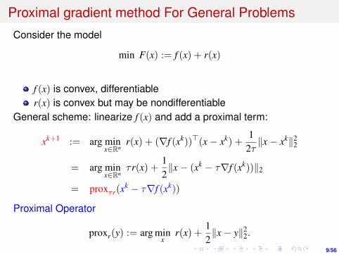
Proximal gradient method For General Problems

Consider the model

min F(x) := f (x) + r(x)

f (x) is convex, differentiabler(x) is convex but may be nondifferentiable

General scheme: linearize f (x) and add a proximal term:

xk+1 := arg minx∈Rn

r(x) + (∇f (xk))>(x− xk) +1

2τ‖x− xk‖2

2

= arg minx∈Rn

τr(x) +12‖x− (xk − τ∇f (xk))‖2

= proxτr(xk − τ∇f (xk))

Proximal Operator

proxr(y) := arg minx

r(x) +12‖x− y‖2

2.

10/56

Proximal mapping

if g is convex and closed (has a closed epigraph), then

proxr(y) := arg minx

r(x) +12‖x− y‖2

2

exists and is unique for all y.from optimality conditions of minimization in the definition:

x = proxr(y) ⇐⇒ y− x ∈ ∂r(x)

⇐⇒ r(z) ≥ r(x) + (y− x)>(z− x), ∀z

subdifferential of a convex function is a monotone operator:

(u− v)>(x− y) ≥ 0 ∀x, y, u ∈ ∂f (x), v ∈ ∂f (y)

proof: combining the following two inequalities

f (y) ≥ f (x) + u>(y− x), f (x) ≥ f (y) + v>(x− y)

11/56

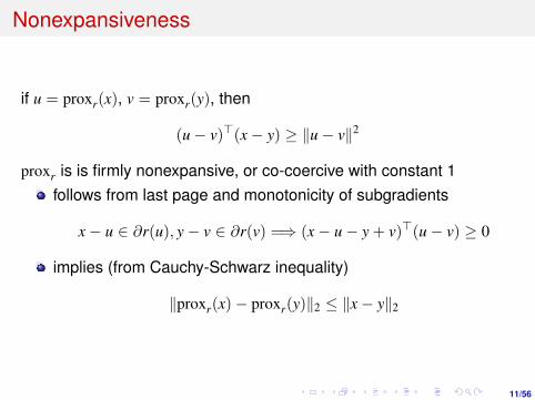
Nonexpansiveness

if u = proxr(x), v = proxr(y), then

(u− v)>(x− y) ≥ ‖u− v‖2

proxr is is firmly nonexpansive, or co-coercive with constant 1follows from last page and monotonicity of subgradients

x− u ∈ ∂r(u), y− v ∈ ∂r(v) =⇒ (x− u− y + v)>(u− v) ≥ 0

implies (from Cauchy-Schwarz inequality)

‖proxr(x)− proxr(y)‖2 ≤ ‖x− y‖2

12/56

Global convergence

The proximal mapping is nonexpansiveUnder certain assumptions, h(x) = x− τ∇f (x) is nonexpansive:

‖h(x)− h(x′)‖ ≤ ‖x− x′‖,

and r(x) = r(x′) whenever the equality holds.x is a fixed point if

‖proxτr(h(x))− proxτr(h(x∗))‖ ≡ ‖proxτr(h(x))− x∗‖ = ‖x− x∗‖

13/56

Proximal gradient method for `1-minimization

AdvantagesLow computational cost (first-order method)Finite convergence of the nondegenerate supportGlobal q-linear convergence

DisadvantagesTakes a lot of steps when the support is relatively largeSlow convergence: degenerate support identification ormagnitude recovery?

Strategies for improving shrinkageAdjust λ dynamically (use λk)Line search xk+1 = xk + αk(shrink(xk − λk∇f k, µλk)− xk)Continuation: approximately solve for µ0 > µ1 > · · · > µp = µ(FPC)Debiasing or subspace optimization

14/56

Line search approach

Let xk(τ k) = shrink(xk − τ k∇f k, µτ k). Then set

xk+1 = xk + αk(xk(τ k)− xk)

= xk + αkdk

Choosing τ k: Barzilai-Borwein method∇f k = A>(Axk − b)sk−1 = xk − xk−1 and yk−1 = ∇f k −∇f k−1

τ k,BB1 = (sk−1)>sk−1

(sk−1)>yk−1 or τ k,BB2 = (sk−1)>yk−1

(yk−1)>yk−1 .

Choosing αk: Armijo-like Line search

ψµ(xk + αkdk) ≤ Ck + σαk∆k

FPC: ∆k := (∇f k)>dk

FPC_AS: ∆k := (∇f k)>dk + µ‖xk(τ k)‖1 − µ‖xk‖1Ck = (ηQk−1Ck−1 + ψµ(xk))/Qk, Qk = ηQk−1 + 1, C0 = ψµ(x0) andQ0 = 1 (Zhang and Hager)

15/56

Outline: Complexity Analysis

Amir Beck and Marc Teboulle, A fast iterative shrinkage thresholdingalgorithm for linear inverse problemsPaul Tseng, On accelerated proximal gradient methods forconvex-concave optimizationPaul Tseng, Approximation accuracy, gradient methods and errorbound for structured convex optimization

N. S. Aybat and G. Iyengar, A first-order augmented Lagrangianmethod for compressed sensing

16/56

Proximal Gradient/ISTA/FPC

The following terminologies refer to the same algorithm:proximal gradient methodISTA: iterative shrinkage thresholding algorithmFPC: fixed-point continuation method

Considermin F(x) := µ‖x‖1 +

12‖Ax− b‖2

2

ISTA/FPC computes

xk+1 := arg minµ‖x‖1 + (∇fk)>(x− xk) +1

2τ‖x− xk‖2

2

= shrink(xk − τ∇fk, µτ)

Complexity?How can we speed it up?

17/56

Generalization of ISTA

Consider a solvable model

min F(x) := f (x) + r(x)

r(x) continuous convex, may be nonsmoothf (x) continuously diff. with Lipschitz continuous gradient

‖∇f (x)−∇f (y)‖2 ≤ Lf ‖x− y‖2

The cost of the following problem is tractable

pL(y) := arg minx

QL(x, y) := f (y) + 〈∇f (y), x− y〉+L2‖x− y‖2

2 + r(x)

= arg minx

r(x) +L2

∥∥∥∥x−(

y− 1L∇f (y)

)∥∥∥∥2

2

= prox1/L(y− 1L∇f (y))

ISTABasic iteration: xk = pL(xk−1)

18/56

Quadratic upper bound

Suppose ∇f is Lipschitz continuous with parameter L and domf isconvex. Then

f (y) ≤ f (x) +∇f (x)>(y− x) +L2‖y− x‖2

2, ∀x, y.

Proof: Let v = y− x. Then

f (y) = f (x) +∇f (x)>v +

∫ 1

0(∇f (x + tv)−∇f (x))>vdt

≤ f (x) +∇f (x)>v +

∫ 1

0‖∇f (x + tv)−∇f (x)‖2‖v‖2dt

≤ f (x) +∇f (x)>v +

∫ 1

0Lt‖v‖2

2dt

= f (x) +∇f (x)>v +L2‖y− x‖2

2

The above inequality also implies that F(pL(y)) ≤ Q(pL(y), y).

19/56

Lemma: Assume F(pL(y)) ≤ Q(pL(y), y), then for any x ∈ Rn,

F(x)− F(pL(y)) ≥ L2‖pL(y)− y‖2 + L 〈y− x, pL(y)− y〉

=L2(‖pL(y)− x‖2

2 − ‖x− y‖22)

Proof: ∇f (y) + L(pL(y)− y) + z = 0 for some z ∈ ∂r(pL(y)).

The convexity of f and g gives

f (x) ≥ f (y) +∇f (y)>(x− y)

r(x) ≥ r(pL(y)) + z>(x− pL(y)).

Using the definition of Q(pL(y), y) and z

F(x)− F(pL(y)) ≥ F(x)− Q(pL(y), y)

≥ −L2‖pL(y)− y‖2 + (x− pL(y))>(∇f (y) + z)

20/56

Complexity analysis of ISTA

Complexity results: F(xk)− F(x∗) ≤ Lf ‖x0−x∗‖22

2k

Let x = x∗, y = xj, then

2L

(F(x∗)− F(xj+1)) ≥ ‖x∗ − xj+1‖22 − ‖x∗ − xj‖2

2

Summing over j := 0, · · · , k − 1 gives

2L

(kF(x∗)−k−1∑j=0

F(xj+1)) ≥ ‖x∗ − xk‖22 − ‖x∗ − x0‖2

2

Let x = y = xj yields2L (F(xj)− F(xj+1)) ≥ ‖xj − xj+1‖2

2Multiplying the last ineq. by j and summing over j := 0, · · · , k − 1 gives

2L (−kF(xk) +

∑k−1j=0 F(xj+1)) ≥

∑k−1j=0 j‖xj − xj+1‖2

2

Therefore2kL (F(x∗)− F(xk)) ≥ ‖x∗ − xk‖2

2 +∑k−1

j=0 j‖xj − xj+1‖22 − ‖x∗ − x0‖2

2

21/56

FISTA: Accelerated proximal gradient

Given y1 = x0 and t1 = 1, compute:

xk = pL(yk)

tk+1 =1 +

√1 + 4t2

k

2

yk+1 = xk +tk − 1tk+1

(xk − xk−1)

Complexity results:

F(xk)− F(x∗) ≤2Lf ‖x0 − x∗‖2

2(k + 1)2

Lipschitz constant Lf is unknown?Choose L by backtracking so that F(pL(yk)) ≤ QL(pL(yk), yk)

22/56

Complexity analysis of FISTA

Let vk := F(xk)− F(x∗) and uk := tkxk − (tk − 1)xk−1 − x∗,

2L

(t2kvk − t2

k+1vk+1)≥ ‖uk+1‖2

2 − ‖uk‖22

If ak − ak+1 ≥ bk+1 − bk, with a1 + b1 ≤ c, then ak ≤ c

tk ≥ (k + 1)/2

Let ak = 2L t2

kvk, bk = ‖uk‖22, and c = ‖x0 − x∗‖2

2.Check a1 + b1 ≤ c:

F(x∗)− F(x1) = F(x∗)− F(pL(y1))

≥ L2‖pL(y1)− y1‖2

2 + L 〈y1 − x∗, pL(y1)− y1〉

=L2

(‖x1 − x∗‖22 − ‖y1 − x∗‖2

2)

23/56

Complexity analysis of FISTA

Let (x = xk, y = yk+1) and (x = x∗, y = yk+1). Note xk+1 = pLk+1 (yk+1):

2L−1(vk − vk+1) ≥ ‖xk+1 − yk+1‖22 + 2 〈xk+1 − yk+1, yk+1 − xk〉 (1)

−2L−1vk+1 ≥ ‖xk+1 − yk+1‖22 + 2 〈xk+1 − yk+1, yk+1 − x∗〉 (2)

((1) ∗ (tk+1 − 1) + (2)) ∗ tk+1 and using t2k = t2

k+1 − tk+1:

2tk+1

L((tk+1 − 1)vk − tk+1vk+1) =

2L

(t2k vk − t2

k+1vk+1)

≥ ‖tk+1(xk+1 − yk+1)‖22 + 2tk+1 〈xk+1 − yk+1, tk+1yk+1 − (tk+1 − 1)xk − x∗〉

‖b− a‖22 + 2 〈b− a, a− c〉 = ‖b− c‖2

2 − ‖a− c‖22

yk+1 = xk + tk−1tk+1

(xk − xk−1):

2L

(t2k vk − t2

k+1vk+1)

≥ ‖tk+1xk+1 − (tk+1 − 1)xk − x∗‖22 − ‖tk+1yk+1 − (tk+1 − 1)xk − x∗‖2

2

= ‖uk+1‖22 − ‖uk‖2

2

24/56

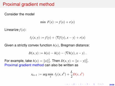
Proximal gradient method

Consider the model

min F(x) := f (x) + r(x)

Linearize f (x):

`f (x, y) := f (y) + 〈∇f (y), x− y〉+ r(x)

Given a strictly convex function h(x), Bregman distance:

D(x, y) := h(x)− h(y)− 〈∇h(y), x− y〉 .

For example, take h(x) = ‖x‖22. Then D(x, y) = ‖x− y‖2

2.Proximal gradient method can also be written as

xk+1 := arg minx

`f (x, xk) +L2

D(x, xk)

25/56

APG Variant 1

Acclerated proximal gradient (APG):Set x−1 = x0 and θ−1 = θ0 = 1:

yk = xk + θk(θ−1k−1 − 1)(xk − xk−1)

xk+1 = arg minx

`f (x, yk) +L2‖x− yk‖2

2

θk+1 =

√θ4

k + 4θ2k − θ2

k

2

Question: what is the difference between θk and tk?

26/56

APG Variant 2

Replace 12‖x− yk‖2

2 by Bregman distance D(x, yk)Set x0, z0 and θ0 = 1:

yk = (1− θk)xk + θkzk

zk+1 = arg minx

`f (x, yk) + θkLD(x, zk)

xk+1 = (1− θk)xk + θkzk+1

θk+1 =

√θ4

k + 4θ2k − θ2

k

2

27/56

APG Variant 3

Set x0, z0 := arg min h(x) and θ0 = 1:

yk = (1− θk)xk + θkzk

zk+1 = arg minx

k∑i=0

`f (x, yi)

θi+ Lh(x)

xk+1 = (1− θk)xk + θkzk+1

θk+1 =

√θ4

k + 4θ2k − θ2

k

2

28/56

Complexity analysis

Proximal gradient method

F(xk) ≤ F(x) +1k

LD(x, x0)

APG1:F(xk) ≤ F(x) +

4(k + 1)2 LD(x, x0)

APG2:F(xk) ≤ F(x) +

4(k + 1)2 LD(x, z0)

APG3:F(xk) ≤ F(x) +

4(k + 1)2 L(h(x)− h(x0))

29/56

Complexity analysis

Let f (x) is convex and assume ∇f (x) is Lipschitz cont.

F(x) ≥ `f (x, y) ≥ F(x)− L2‖x− y‖2

2.

For any proper lsc convex function ψ(x), if z+ = arg minx ψ(x) + D(x, z)and h(x) is differentiable at z+, then

ψ(x) + D(x, z) ≥ ψ(z+) + D(x, z+) + D(z+, z).

Proof: The optimality at z+ and definition of subgradient gives

ψ(x) +∇xD(z+, z)>(x− z+) ≥ ψ(z+).

Note ∇xD(z+, z) = ∇h(z+)−∇h(z). Rearranging terms yields

ψ(x)−∇h(z)>(x− z) ≥ ψ(z+)−∇h(z)>(z+ − z)−∇h(z+)>(x− z+).

Adding h(x)− h(z) to both sides.

30/56

Complexity analysis of APG2

F(xk+1)

≤ `f (xk+1, yk) +L2‖xk+1 − yk‖2

2

= `f ((1− θk)xk + θzk+1, yk) +Lθ2

k2‖zk+1 − zk‖2

2

≤ (1− θk)`f (xk, yk) + θk`f (zk+1, yk) + θ2k LD(zk+1, zk)

≤ (1− θk)`f (xk, yk) + θk (`f (x, yk) + θkLD(x, zk)− θkLD(x, zk+1))

≤ (1− θk)F(xk) + θkF(x) + θ2k LD(x, zk)− θ2

k LD(x, zk+1)

The third inequality applies the inequality for `f (x, z) + θLD(x, z).

Let ek = F(xk)− F(x) and ∆k = LD(x, zk),then

ek+1 ≤ (1− θk)ek + θ2k∆k − θ2

k∆k+1

31/56

Complexity analysis of APG2

Divide both sides by θ2k and using 1

θ2k

=1−θk+1θ2

k+1:

1− θk+1

θ2k+1

ek+1 + ∆k+1 ≤1− θk

θ2k

ek + ∆k

Hence1− θk+1

θ2k+1

ek+1 + ∆k+1 ≤1− θ0

θ20

e0 + ∆0

Using 1θ2

k=

1−θk+1θ2

k+1and θ0 = 1:

1θ2

kek+1 ≤ ∆0 −∆k+1 ≤ ∆0 = LD(x, z0)

32/56

An application to Basis Pursuit problem

Considermin ‖x‖1 s.t. Ax = b

Augmented Lagragian (Bregman) framework (b1 = b, k = 1):

x∗k := arg minx

Fk(x) := µk‖x‖1 +12‖Ax− bk‖2

2

bk+1 := b +µk+1

µk(bk − Axk)

obtaining x∗k+1 exactly is difficultinexact solver: how do we control the accuracy?Analysis of Bregman approach (see wotao), no complexitySolving each x∗k+1 by the APG algorithms?

33/56

Outline: ADMM

Alternating direction augmented Lagrangian methodsVariable splitting methodConvergence for problems with two blocks of variables

34/56

References

Wotao Yin, Stanley Osher, Donald Goldfarb, Jerome Darbon,Bregman Iterative Algorithms for l1-Minimization withApplications to Compressed SensingJunfeng Yang, Yin Zhang, Alternating direction algorithms forl1-problems in Compressed SensingTom Goldstein, Stanely Osher, The Split Bregman Method forL1-Regularized ProblemsB.S. He, H. Yang, S.L. Wang, Alternating Direction Method withSelf-Adaptive Penalty Parameters for Monotone VariationalInequalities

35/56

Basis pursuit problem

Primal: min ‖x‖1, s.t. Ax = b

Dual: max b>λ, s.t. ‖A>λ‖∞ ≤ 1

The dual problem is equivalent to

max b>λ, s.t. A>λ = s, ‖s‖∞ ≤ 1.

36/56

Augmented Lagrangian (Bregman) framework

Augmented Lagrangian function:

L(λ, s, x) := −b>λ+ x>(A>λ− s) +1

2µ‖A>λ− s‖2

Algorithmic frameworkCompute λk+1 and sk+1 at k-th iteration

(DL) minλ,s L(λ, s, xk), s.t. ‖s‖∞ ≤ 1

Update the Lagrangian multiplier:xk+1 = xk + A>λk+1−sk+1

µ

Pros and Cons:Pros: rich theory, well understood and a lot of algorithmsCons: L(λ, s, xk) is not separable in λ and s, and the subproblem(DL) is difficult to minimize

37/56

An alternating direction minimization scheme

Divide variables into different blocks according to their rolesMinimize the augmented Lagrangian function with respect to oneblock at a time while all other blocks are fixed

ADMM

λk+1 = arg minλL(λ, sk, xk)

sk+1 = arg minsL(λk+1, s, xk), s.t. ‖s‖∞ ≤ 1

xk+1 = xk +A>λk+1 − sk+1

µ

38/56

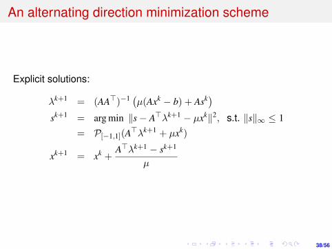
An alternating direction minimization scheme

Explicit solutions:

λk+1 = (AA>)−1 (µ(Axk − b) + Ask)sk+1 = arg min ‖s− A>λk+1 − µxk‖2, s.t. ‖s‖∞ ≤ 1

= P[−1,1](A>λk+1 + µxk)

xk+1 = xk +A>λk+1 − sk+1

µ

39/56

ADMM for BP-denoising

Primal:min ‖x‖1, s.t. ‖Ax− b‖2 ≤ σ

which is equivalent to

min ‖x‖1, s.t. Ax− b + r = 0, ‖r‖2 ≤ σ

Lagrangian function:

L(x, r, λ) := ‖x‖1 − λ>(Ax− b + r) + π(‖r‖2 − σ)

= ‖x‖1 − (A>λ)>x + π‖r‖2 − λ>r + b>λ− πσ

Hence, the dual problem is:

max b>λ− πσ, s.t. ‖A>λ‖∞ ≤ 1, ‖λ‖2 ≤ π

40/56

ADMM for BP-denoising

The dual problem is equivalent to:

max b>λ− πσ, s.t. A>λ = s, ‖s‖∞ ≤ 1, ‖λ‖2 ≤ π

Augmented Lagrangian function is:

L(λ, s, x) := −b>λ+ πσ + x>(A>λ− s) +1

2µ‖A>λ− s‖2

ADMM scheme:

λk+1 = arg min1

2µ‖A>λ− sk‖2 + (Axk − b)>λ, s.t. ‖λ‖2 ≤ πk

sk+1 = arg min ‖s− A>λk+1 − µxk‖2, s.t. ‖s‖∞ ≤ 1

= P[−1,1](A>λk+1 + µxk)

πk+1 = ‖λk+1‖2

xk+1 = xk +A>λk+1 − sk+1

µ

41/56

ADMM for `1-regularized problem

Primal:min µ‖x‖1 +

12‖Ax− b‖2

2

which is equivalent to

min µ‖x‖1 +12‖r‖2

2, s.t. Ax− b = r.

Lagrangian function:

L(x, r, λ) := µ‖x‖1 +12‖r‖2

2 − λ>(Ax− b− r)

= µ‖x‖1 − (A>λ)>x +12‖r‖2

2 + λ>r + b>λ

Hence, the dual problem is:

max b>λ− 12‖λ‖2, s.t. ‖A>λ‖∞ ≤ µ

42/56

ADMM for `1-regularized problem

The dual problem is equivalent to

max b>λ− 12‖λ‖2, s.t. A>λ = s, ‖s‖∞ ≤ µ.

Augmented Lagrangian function is:

L(λ, s, x) := −b>λ+12‖λ‖2 + x>(A>λ− s) +

12µ‖A>λ− s‖2

ADMM scheme:

λk+1 = (AA> + µI)−1 (µ(Axk − b) + Ask)sk+1 = arg min ‖s− A>λk+1 − µxk‖2, s.t. ‖s‖∞ ≤ µ

= P[−µ,µ](A>λk+1 + µxk)

xk+1 = xk +A>λk+1 − sk+1

µ

43/56

YALL1

Derive ADMM for the following problems:

BP: minx∈Cn ‖Wx‖w,1, s.t. Ax = b

L1/L1: minx∈Cn ‖Wx‖w,1 +1ν‖Ax− b‖1

L1/L2: minx∈Cn ‖Wx‖w,1 +1

2ρ‖Ax− b‖2

2

BP+: minx∈Rn ‖x‖w,1, s.t. Ax = b, x ≥ 0

L1/L1+: minx∈Rn ‖x‖w,1 +1ν‖Ax− b‖1, s.t. x ≥ 0

L1/L2+: minx∈Rn ‖x‖w,1 +1

2ρ‖Ax− b‖2

2, s.t. x ≥ 0

ν, ρ ≥ 0, A ∈ Cm×n, b ∈ Cm,x ∈ Cn for the first three and x ∈ Rn for thelast three, W ∈ Cn×n is an unitary matrix serving as a sparsifyingbasis, and ‖x‖w,1 :=

∑ni=1 wi|xi|.

44/56

Variable splitting

Given A ∈ Rm×n, consider min f (x) + g(Ax), which is

min f (x) + g(y), s.t. Ax = y

Augmented Lagrangian function:

L(x, y, λ) = f (x) + g(y)− λ>(Ax− y) +1

2µ‖Ax− y‖2

2

ADMM

(Px) : xk+1 := arg minx∈X

L(x, yk, λk),

(Py) : yk+1 := arg miny∈Y

L(xk+1, y, λk),

(Pλ) : λk+1 := λk − γAxk+1 − yk+1

µ

45/56

Variable splitting

split Bregman (Goldstein and Osher) for anisotropic TV:

min α‖Du‖1 + β‖Ψu‖1 +12‖Au− f‖2

2

Introduce y = Du and w = Ψu, obtain

min α‖y‖1 + β‖w‖1 +12‖Au− f‖2

2, s.t. y = Du, w = Ψu

Augmented Lagrangian function:

L := α‖y‖1 + β‖w‖1 +12‖Au− f‖2

2 − p>(Du− y) +1

2µ‖Du− y‖2

2

−q>(Ψu− w) +1

2µ‖Ψu− w‖2

2

46/56

Variable splitting

The variable u can be otained by(A>A +

1µ

(D>D + I))

u = A>f +1µ

(D>y + Ψ>w) + D>p + Ψ>q

If A and D are diagonalizable by FFT, then the computationalcost is very cheap. For example, A = RF , both R and D arecirculant matrices.Variables y and w:

y := shrink(Du− µp, αµ)

w := shrink(Ψu− µq, αµ)

apply a few iterations before updating the Lagrangian multipliersp and q

Exercise: isotropic TV

min α‖Du‖2 + β‖Ψu‖1 +12‖Au− f‖2

2

47/56

FTVd: Fast TV deconvolution

Wang-Yang-Yin-Zhang consider:

minu

∑‖Diu‖2 +

12µ‖Ku− f‖2

2

Introducing w and quadratic penalty:

minu,w

∑(‖wi‖2 +

12β‖wi − Diu‖2

2

)+

12µ‖Ku− f‖2

2

Alternating minimization:For fixed u, {wi} can be solved by shrinkage at O(N)

For fixed {wi}, u can be solved by FFT at O(N log N)

48/56

Outline: Linearized ADMM

Linearized Bregman and Bregmanized operator splittingADMM + proximal point methodXiaoqun Zhang, Martin Burgerz, Stanley Osher, A unifiedprimal-dual algorithm framework based on Bregman iteration

49/56

Review of Bregman method

Consider BP:min ‖x‖1, s.t. Ax = b

Bregman method:

Dpk

J (x, xk) := ‖x‖1 − ‖xk‖1 −⟨pk, x− xk

⟩xk+1 := arg minx µDpk

J (x, xk) + 12‖Ax− b‖2

2

pk+1 = pk + 1µA>(b− Axk+1)

Augmented Lagrangian (updating multiplier or b):xk+1 := arg minx µ‖x‖1 + 1

2‖Ax− bk‖22

bk+1 = b + (bk − Axk+1)

They are equivalent, see Yin-Osher-Goldfarb-Darbon

50/56

Linearized approaches

Linearized Bregman method:

xk+1 := arg min µDpk

J (x, xk) + (A>(Axk − b))>(x− xk) +12δ‖x− xk‖2

2,

pk+1 := pk − 1µδ

(xk+1 − xk)− 1µ

A>(Axk − b),

which is equivalent to

xk+1 := arg min µ‖x‖1 +12δ‖x− vk‖2

2

vk+1 := vk − δA>(Axk+1 − b)

Bregmanized operator splitting:

xk+1 := arg min µ‖x‖1 + (A>(Axk − bk))>(x− xk) +12δ‖x− xk‖2

2

bk+1 = b + (bk − Axk+1)

Are they equivalent?

50/56

Linearized approaches

Linearized Bregman method:

xk+1 := arg min µDpk

J (x, xk) + (A>(Axk − b))>(x− xk) +12δ‖x− xk‖2

2,

pk+1 := pk − 1µδ

(xk+1 − xk)− 1µ

A>(Axk − b),

which is equivalent to

xk+1 := shrink(vk, µδ)

vk+1 := vk − δA>(Axk+1 − b)or

xk+1 := shrink(δA>bk, µδ)

bk+1 := b + (bk − Axk+1)

Bregmanized operator splitting:

xk+1 := shrink(xk − δ(A>(Axk − bk)), µδ) = shrink(δA>bk + xk − δA>Axk, µδ)

bk+1 = b + (bk − Axk+1)

51/56

Linearized approaches

Linearized Bregman:If the sequence xk converges and pk is bounded, then the limit ofxk is the unique solution of

min µ‖x‖1 +12δ‖x‖2

2 s.t. Ax = b.

For µ large enough, the limit solution solves BP.Exact regularization if δ > δ̄

What about Bregmanized operator splitting?

52/56

Primal ADMM for `1-regularized problem

Primal: min µ‖x‖1 + 12‖Ax− b‖2

2 which is equivalent to

min µ‖x‖1 +12‖r‖2

2, s.t. Ax− b = r.

Augmented Lagrangian function:

L(x, r, λ) = µ‖x‖1 +12‖r‖2

2 − λ>(Ax− b− r) +12δ‖Ax− b− r‖2

2

ADMM scheme:

xk+1 = arg minx

µ‖x‖1 +12δ‖Ax− b− rk − δλk‖2

2 original problem

rk+1 = arg minr

12‖r‖2

2 +12δ‖Axk+1 − b− r − δλk‖2

2

λk+1 = λk +Axk+1 − b− rk+1

δ

52/56

Primal ADMM for `1-regularized problem

Primal: min µ‖x‖1 + 12‖Ax− b‖2

2 which is equivalent to

min µ‖x‖1 +12‖r‖2

2, s.t. Ax− b = r.

Augmented Lagrangian function:

L(x, r, λ) = µ‖x‖1 +12‖r‖2

2 − λ>(Ax− b− r) +12δ‖Ax− b− r‖2

2

ADMM scheme:

xk+1 = arg minx

µ‖x‖1 + (gk)>(x− xk) +1

2τ‖x− xk‖2

2

rk+1 = arg minr

12‖r‖2

2 +12δ‖Axk+1 − b− r − δλk‖2

2

λk+1 = λk +Axk+1 − b− rk+1

δ

Convergence of the linearized scheme?

53/56

Generalized algorithm

Considermin f (x), s.t. Ax = b

Proximal-point method:

xk+1 := arg minx

f (x)−⟨λk,Ax− b

⟩+

12δ‖Ax− b‖2 +

12‖x− xk‖2

Q

Cλk+1 := Cλk + (b− Axk+1)

Augmented Lagrangian or Bregman method if Q = 0 and C = δ

Proximal point method by Rockafellar if Q = I and C = γ

Bregmanized operator splitting if Q = 1δ(I − A>A)

Theoretical results: limk ‖Axk − b‖2 = 0, limk f (xk) = f (x̄) and all limitpoint of (xk, λk) are saddle points.

54/56

Convergence proof

From the x-subproblem:

∂f (xk+1) 3 sk+1 := A>λk − 1δ

A>(Axk+1 − b)− Q(xk+1 − xk)

Assume (x̄, λ̄) is a saddle point, then Ax̄ = b, and s̄− A>λ̄ = 0.Let sk+1

e = sk+1 − s̄, xk+1e = xk+1 − x̄ and λk+1

e = λk+1 − λ̄:

sk+1e +

1δ

A>Axk+1e + Qxk+1

e = Qxke + A>λk

e, Cλk+1e = Cλk

e − Axk+1e

Taking the inner product with xk+1e on both sides of the first equality:

12

(‖xk+1

e ‖2Q + ‖xk+1 − xk‖2

Q − ‖xke‖2

Q

)= −

⟨sk+1

e , xk+1e

⟩− 1δ‖Axk+1

e ‖22 +

⟨λk

e,Axk+1e

⟩Taking the inner product with λk+1

e on both sides of the second equality:

12

(‖λk+1

e ‖2C − ‖λk

e‖2C − ‖Axk+1

e ‖2C−1

)= −

⟨λk

e,Axk+1e

⟩Adding the above inequality (wk = (xk, λk)):

‖wk+1e ‖2

Q + ‖xk+1 − xk‖2Q + 2

⟨sk+1

e , xk+1e

⟩+

2δ‖Axk+1

e ‖22 − ‖Axk+1

e ‖2C−1 = ‖wk

e‖2Q

55/56

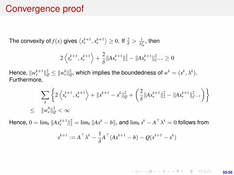
Convergence proof

The convexity of f (x) gives⟨sk+1

e , xk+1e⟩≥ 0. If 2

δ> 1

λCm

, then

2⟨

sk+1e , xk+1

e

⟩+

2δ‖Axk+1

e ‖22 − ‖Axk+1

e ‖2C−1 ≥ 0

Hence, ‖wk+1e ‖2

Q ≤ ‖wke‖2

Q, which implies the boundedness of wk = (xk, λk).Furthermore,∑

k

{2⟨

sk+1e , xk+1

e

⟩+ ‖xk+1 − xk‖2

Q +

(2δ‖Axk+1

e ‖22 − ‖Axk+1

e ‖2C−1

)}≤ ‖w0

e‖2Q <∞

Hence, 0 = limk ‖Axk+1e ‖2

2 = limk ‖Axk − b‖, and limk sk − A>λk = 0 follows from

sk+1 := A>λk − 1δ

A>(Axk+1 − b)− Q(xk+1 − xk)

56/56

Generalized algorithm

Considermin f (x) + g(z), s.t. Bx = z

Proximal-point method:

xk+1 := arg minx

f (x)−⟨λk,Bx

⟩+

12δ‖Bx− zk‖2 +

12‖x− xk‖2

Q

zk+1 := arg minz

g(z)−⟨λk, z

⟩+

12δ‖Bxk+1 − z‖2 +

12‖z− zk‖2

M

Cλk+1 := Cλk + (Bxk+1 − zk+1)

ADMM if Q = M = 0 and C = δ

Proximal point method by Rockafellar if Q = I and C = γ

Bregmanized operator splitting if Q = 1δ(I − A>A)

Theoretical results: limk ‖Bxk − zk‖2 = 0, limk f (xk) = f (x̄) ,limk g(zk) = g(z̄) and all limit point of (xk, zk, λk) are saddle points.