Embed Size (px)
Citation preview
Recursive Compressed Sensing
Pantelis Sopasakis∗
Presentation at ICTEAM – UC Louvain, Belgiumjoint work with N. Freris† and P. Patrinos‡
∗ IMT Institute for advanced studies Lucca, Italy† NYU, Abu Dhabi, United Arab Emirates
‡ ESAT, KU Leuven, Belgium
April 7, 2016
Motivation
MRI
Radio-astronomy
Holography
Seismology
Photography
RadarsFa
cial
rec
ogni
tion
Speech recognition
Fault detection
Medicalimaging
Faci
al r
ecog
nitio
n
Part
icle
phy
sics
Video processing
ECG
Encr
yptio
n
Communication networks
System identification
Compressed Sensing
1 / 55
Spoiler alert!
The proposed method is an order of magnitude faster compared toother reported methods for recursive compressed sensing.
2 / 55
Outline
1. Forward-Backward Splitting
2. The Forward-Backward envelope function
3. The Forward-Backward Newton method
4. Recursive compressed sensing
5. Simulations
3 / 55

I. Forward-Backward Splitting
Forward-Backward Splitting
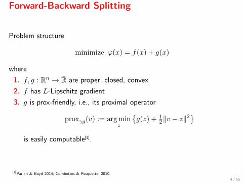
Problem structure
minimize ϕ(x) = f(x) + g(x)
where
1. f, g : Rn → R are proper, closed, convex
2. f has L-Lipschitz gradient
3. g is prox-friendly, i.e., its proximal operator
proxγg(v) := arg minz
{g(z) + 1
2‖v − z‖2}
is easily computable[1].
[1]Parikh & Boyd 2014; Combettes & Pesquette, 2010.
4 / 55
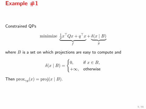
Example #1
Constrained QPs
minimize 12x>Qx+ q>x︸ ︷︷ ︸
f
+ δ(x | B)︸ ︷︷ ︸g
where B is a set on which projections are easy to compute and
δ(x | B) =
{0, if x ∈ B,+∞, otherwise
Then proxγg(x) = proj(x | B).
5 / 55
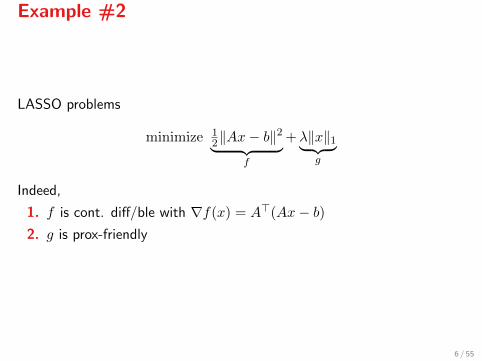
Example #2
LASSO problems
minimize 12‖Ax− b‖
2︸ ︷︷ ︸f
+λ‖x‖1︸ ︷︷ ︸g
Indeed,
1. f is cont. diff/ble with ∇f(x) = A>(Ax− b)2. g is prox-friendly
6 / 55
Other examples
X Constrained optimal control
X Elastic net
X Sparse log-logistic regression
X Matrix completion
X Subspace identification
X Support vector machines
7 / 55
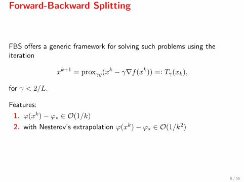
Forward-Backward Splitting
FBS offers a generic framework for solving such problems using theiteration
xk+1 = proxγg(xk − γ∇f(xk)) =: Tγ(xk),
for γ < 2/L.
Features:
1. ϕ(xk)− ϕ? ∈ O(1/k)
2. with Nesterov’s extrapolation ϕ(xk)− ϕ? ∈ O(1/k2)
8 / 55
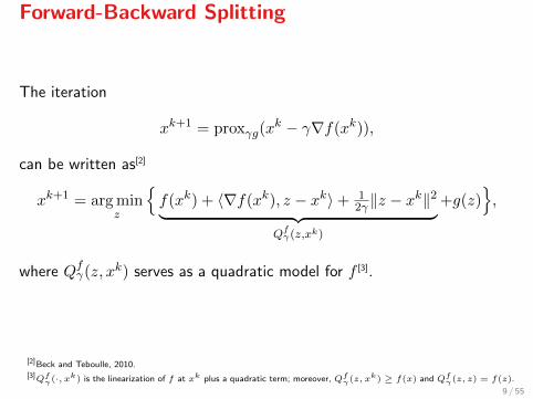
Forward-Backward Splitting
The iteration
xk+1 = proxγg(xk − γ∇f(xk)),
can be written as[2]
xk+1 = arg minz
{f(xk) + 〈∇f(xk), z − xk〉+ 1
2γ ‖z − xk‖2︸ ︷︷ ︸
Qfγ(z,xk)
+g(z)},
where Qfγ(z, xk) serves as a quadratic model for f [3].
[2]Beck and Teboulle, 2010.[3]Qfγ(·, x
k) is the linearization of f at xk plus a quadratic term; moreover, Qfγ(z, xk) ≥ f(x) and Qfγ(z, z) = f(z).
9 / 55
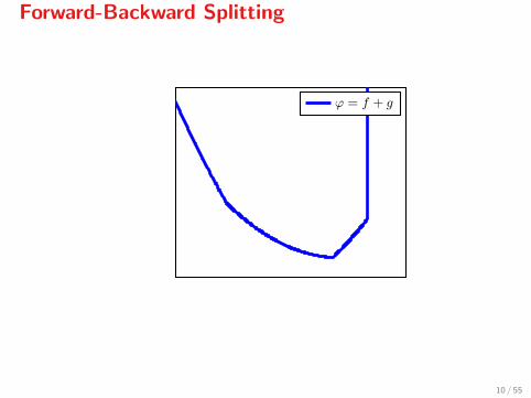
Forward-Backward Splitting
x0
ϕ(x0)
ϕ = f + g
10 / 55

Forward-Backward Splitting
x0
ϕ(x0)
ϕ = f + g
11 / 55

Forward-Backward Splitting
x0
ϕ(x0)
ϕ = f + g
Qfγ(z;x
0) + g(z)
12 / 55
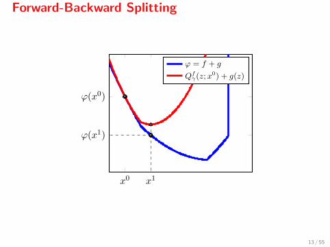
Forward-Backward Splitting
x0 x1
ϕ(x0)
ϕ(x1)
ϕ = f + g
Qfγ(z;x
0) + g(z)
13 / 55
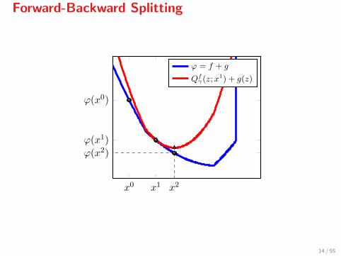
Forward-Backward Splitting
x0 x1 x2
ϕ(x0)
ϕ(x1)
ϕ(x2)
ϕ = f + g
Qfγ(z;x
1) + g(z)
14 / 55
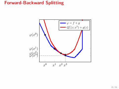
Forward-Backward Splitting
x0 x1 x2 x3
ϕ(x0)
ϕ(x1)
ϕ(x2)ϕ(x3)
ϕ = f + g
Qfγ(z;x
2) + g(z)
15 / 55
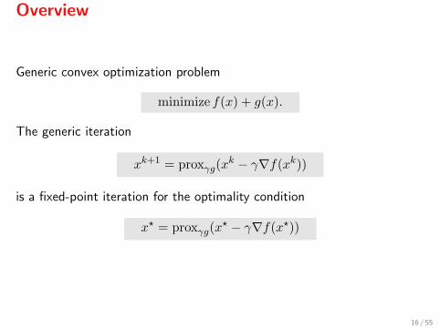
Overview
Generic convex optimization problem
minimize f(x) + g(x).
The generic iteration
xk+1 = proxγg(xk − γ∇f(xk))
is a fixed-point iteration for the optimality condition
x? = proxγg(x? − γ∇f(x?))
16 / 55
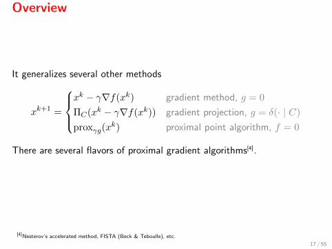
Overview
It generalizes several other methods
xk+1 =
xk − γ∇f(xk) gradient method, g = 0
ΠC(xk − γ∇f(xk)) gradient projection, g = δ(· | C)
proxγg(xk) proximal point algorithm, f = 0
There are several flavors of proximal gradient algorithms[4].
[4]Nesterov’s accelerated method, FISTA (Beck & Teboulle), etc.
17 / 55
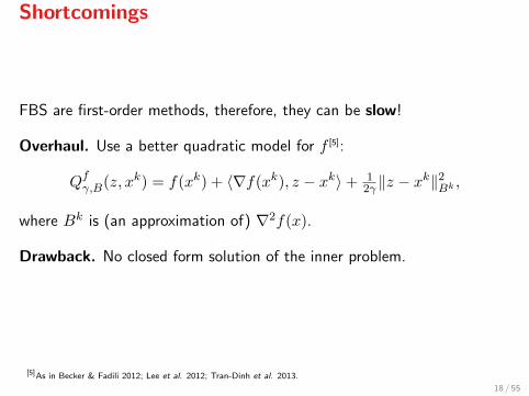
Shortcomings
FBS are first-order methods, therefore, they can be slow!
Overhaul. Use a better quadratic model for f [5]:
Qfγ,B(z, xk) = f(xk) + 〈∇f(xk), z − xk〉+ 12γ ‖z − x
k‖2Bk ,
where Bk is (an approximation of) ∇2f(x).
Drawback. No closed form solution of the inner problem.
[5]As in Becker & Fadili 2012; Lee et al. 2012; Tran-Dinh et al. 2013.
18 / 55

II. Forward-Backward Envelope

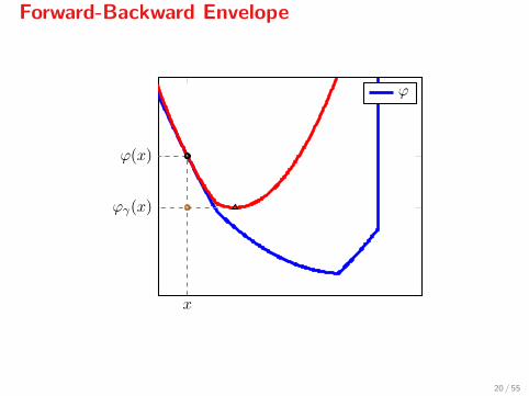
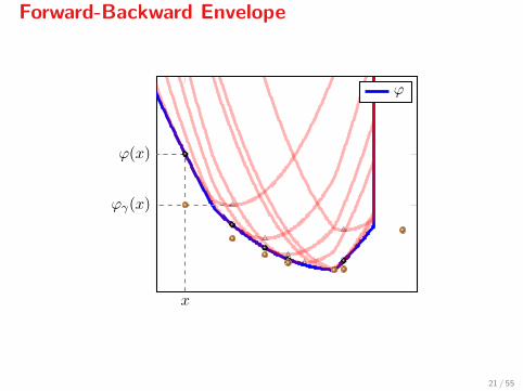
Forward-Backward Envelope
The Forward-Backward envelope of ϕ is defined as
ϕγ(x) = minz
{f(x) + 〈∇f(x), z − x〉+ g(z) + 1
2γ ‖z − x‖2},
with γ ≤ 1/L. Let’s see how it looks...
19 / 55
Forward-Backward Envelope
x
ϕ(x)
ϕγ(x)
ϕ
20 / 55
Forward-Backward Envelope
x
ϕ(x)
ϕγ(x)
ϕ
21 / 55
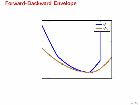
Forward-Backward Envelope
x
ϕ(x)
ϕγ(x)
ϕϕγ
22 / 55
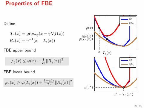
Properties of FBE
Define
Tγ(x) = proxγg(x− γ∇f(x))
Rγ(x) = γ−1(x− Tγ(x))
FBE upper bound
ϕγ(x) ≤ ϕ(x)− 12γ ‖Rγ(x)‖2
FBE lower bound
ϕγ(x) ≥ ϕ(Tγ(x)) +1−γLf
2γ ‖Rγ(x)‖2
x Tγ(x)
ϕ(x)
ϕ(Tγ(x))ϕγ(x)
ϕϕγ
x? = Tγ(x?)
ϕ(x?)
ϕϕγ
23 / 55

Properties of FBE
Ergo: Minimizing ϕ is equivalent to minimizing its FBE ϕγ .
inf ϕ = inf ϕγ
arg minϕ = arg minϕγ
However, ϕγ is continuously diff/able[6] whenever f ∈ C2.
[6]More about the FBE: P. Patrinos, L. Stella and A. Bemporad, 2014.
24 / 55
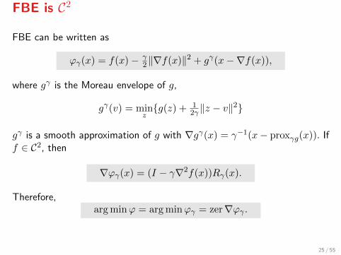
FBE is C2
FBE can be written as
ϕγ(x) = f(x)− γ2‖∇f(x)‖2 + gγ(x−∇f(x)),
where gγ is the Moreau envelope of g,
gγ(v) = minz{g(z) + 1
2γ ‖z − v‖2}
gγ is a smooth approximation of g with ∇gγ(x) = γ−1(x− proxγg(x)). Iff ∈ C2, then
∇ϕγ(x) = (I − γ∇2f(x))Rγ(x).
Therefore,arg minϕ = arg minϕγ = zer∇ϕγ .
25 / 55
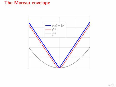
The Moreau envelope
g(x) = |x|g0.1
g10
26 / 55
Forward-Backward Newton
X Since ϕγ is C1 but not C2, we may not apply a Newton method.
X The FB Newton method is a semi-smooth method for minimizing ϕγusing a notion of generalized differentiability.
X The FBN iterations are
xk+1 = xk + τkdk,
where dk is a Newton direction given by
Hkdk = −∇ϕγ(xk),
Hk ∈ ∂2Bϕγ(xk),
X ∂B is the so-called B-subdifferential (we’ll define it later)
27 / 55

III. Forward-Backward Newton
Optimality conditions
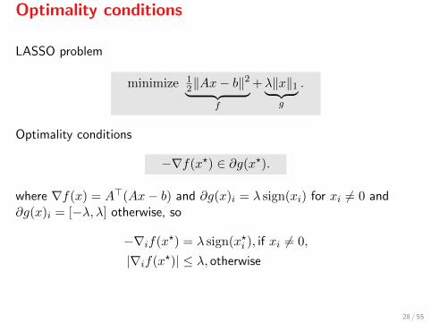
LASSO problem
minimize 12‖Ax− b‖
2︸ ︷︷ ︸f
+λ‖x‖1︸ ︷︷ ︸g
.
Optimality conditions
−∇f(x?) ∈ ∂g(x?).
where ∇f(x) = A>(Ax− b) and ∂g(x)i = λ sign(xi) for xi 6= 0 and∂g(x)i = [−λ, λ] otherwise, so
−∇if(x?) = λ sign(x?i ), if xi 6= 0,
|∇if(x?)| ≤ λ, otherwise
28 / 55

Optimality conditions
If we knew the set
α = {i : x?i = 0},β = {j : x?j 6= 0},
we would be able to write down the optimality conditions as
A>αAαx?α = A>α b+ λ sign(x?α)
Goal. Devise a method to determine α efficiently.
29 / 55
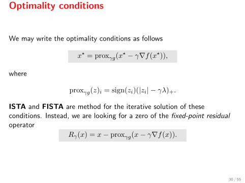
Optimality conditions
We may write the optimality conditions as follows
x? = proxγg(x? − γ∇f(x?)),
where
proxγg(z)i = sign(zi)(|zi| − γλ)+.
ISTA and FISTA are method for the iterative solution of theseconditions. Instead, we are looking for a zero of the fixed-point residualoperator
Rγ(x) = x− proxγg(x− γ∇f(x)).
30 / 55
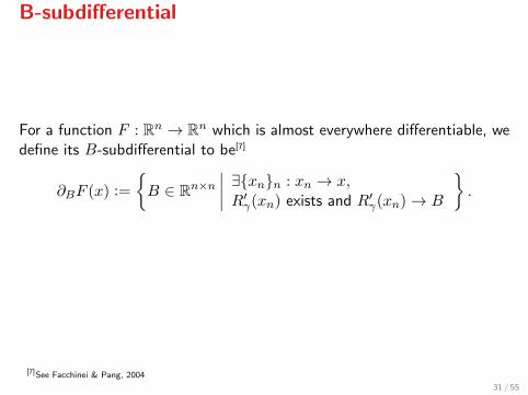
B-subdifferential
For a function F : Rn → Rn which is almost everywhere differentiable, wedefine its B-subdifferential to be[7]
∂BF (x) :=
{B ∈ Rn×n
∣∣∣∣ ∃{xn}n : xn → x,R′γ(xn) exists and R′γ(xn)→ B
}.
[7]See Facchinei & Pang, 2004
31 / 55
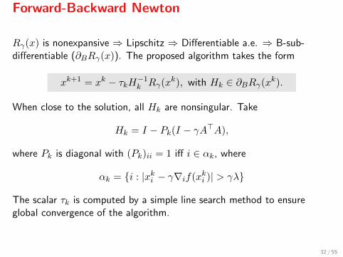
Forward-Backward Newton
Rγ(x) is nonexpansive ⇒ Lipschitz ⇒ Differentiable a.e. ⇒ B-sub-differentiable (∂BRγ(x)). The proposed algorithm takes the form
xk+1 = xk − τkH−1k Rγ(xk), with Hk ∈ ∂BRγ(xk).
When close to the solution, all Hk are nonsingular. Take
Hk = I − Pk(I − γA>A),
where Pk is diagonal with (Pk)ii = 1 iff i ∈ αk, where
αk = {i : |xki − γ∇if(xki )| > γλ}
The scalar τk is computed by a simple line search method to ensureglobal convergence of the algorithm.
32 / 55
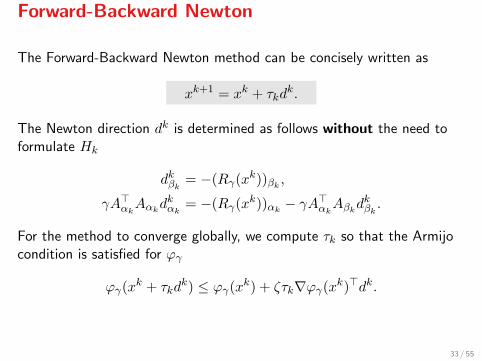
Forward-Backward Newton
The Forward-Backward Newton method can be concisely written as
xk+1 = xk + τkdk.
The Newton direction dk is determined as follows without the need toformulate Hk
dkβk = −(Rγ(xk))βk ,
γA>αkAαkdkαk
= −(Rγ(xk))αk − γA>αkAβkd
kβk.
For the method to converge globally, we compute τk so that the Armijocondition is satisfied for ϕγ
ϕγ(xk + τkdk) ≤ ϕγ(xk) + ζτk∇ϕγ(xk)>dk.
33 / 55
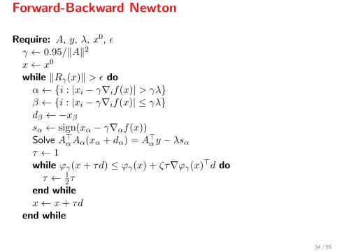
Forward-Backward Newton
Require: A, y, λ, x0, εγ ← 0.95/‖A‖2x← x0
while ‖Rγ(x)‖ > ε doα← {i : |xi − γ∇if(x)| > γλ}β ← {i : |xi − γ∇if(x)| ≤ γλ}dβ ← −xβsα ← sign(xα − γ∇αf(x))Solve A>αAα(xα + dα) = A>α y − λsατ ← 1while ϕγ(x+ τd) ≤ ϕγ(x) + ζτ∇ϕγ(x)>d doτ ← 1
2τend whilex← x+ τd
end while
34 / 55

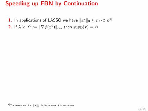
Speeding up FBN by Continuation
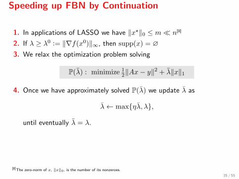
1. In applications of LASSO we have ‖x?‖0 ≤ m� n[8]
2. If λ ≥ λ0 := ‖∇f(x0)‖∞, then supp(x) = ∅3. We relax the optimization problem solving
P(λ) : minimize 12‖Ax− y‖
2 + λ‖x‖1
4. Once we have approximately solved P(λ) we update λ as
λ← max{ηλ, λ},
until eventually λ = λ.
5. This way we enforce that (i) |αk| increases smoothly, (ii) |αk| < m,(iii) A>αkAαk remains always positive definite.
[8]The zero-norm of x, ‖x‖0, is the number of its nonzeroes.
35 / 55
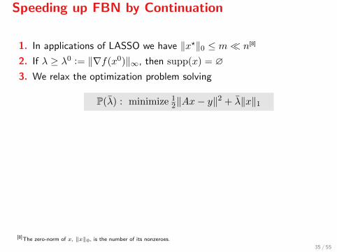
Speeding up FBN by Continuation
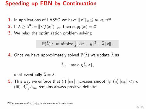
1. In applications of LASSO we have ‖x?‖0 ≤ m� n[8]
2. If λ ≥ λ0 := ‖∇f(x0)‖∞, then supp(x) = ∅
3. We relax the optimization problem solving
P(λ) : minimize 12‖Ax− y‖
2 + λ‖x‖1
4. Once we have approximately solved P(λ) we update λ as
λ← max{ηλ, λ},
until eventually λ = λ.
5. This way we enforce that (i) |αk| increases smoothly, (ii) |αk| < m,(iii) A>αkAαk remains always positive definite.
[8]The zero-norm of x, ‖x‖0, is the number of its nonzeroes.
35 / 55
Speeding up FBN by Continuation
1. In applications of LASSO we have ‖x?‖0 ≤ m� n[8]
2. If λ ≥ λ0 := ‖∇f(x0)‖∞, then supp(x) = ∅3. We relax the optimization problem solving
P(λ) : minimize 12‖Ax− y‖
2 + λ‖x‖1
4. Once we have approximately solved P(λ) we update λ as
λ← max{ηλ, λ},
until eventually λ = λ.
5. This way we enforce that (i) |αk| increases smoothly, (ii) |αk| < m,(iii) A>αkAαk remains always positive definite.
[8]The zero-norm of x, ‖x‖0, is the number of its nonzeroes.
35 / 55
Speeding up FBN by Continuation
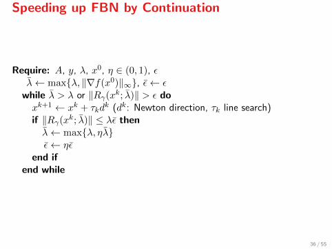
Require: A, y, λ, x0, η ∈ (0, 1), ελ← max{λ, ‖∇f(x0)‖∞}, ε← ε
while λ > λ or ‖Rγ(xk; λ)‖ > ε doxk+1 ← xk + τkd
k (dk: Newton direction, τk line search)if ‖Rγ(xk; λ)‖ ≤ λε thenλ← max{λ, ηλ}ε← ηε
end ifend while
36 / 55
Further speed up
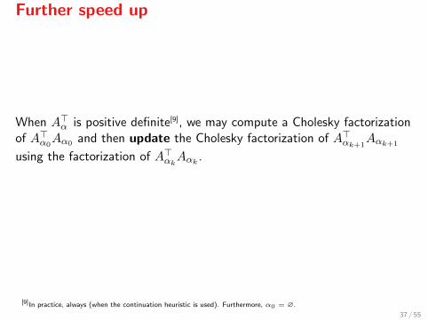
When A>α is positive definite[9], we may compute a Cholesky factorizationof A>α0
Aα0 and then update the Cholesky factorization of A>αk+1Aαk+1
using the factorization of A>αkAαk .
[9]In practice, always (when the continuation heuristic is used). Furthermore, α0 = ∅.
37 / 55
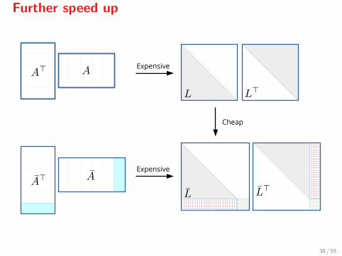
Further speed up
Cheap
Expensive
Expensive
38 / 55
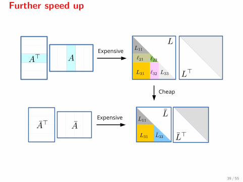
Further speed up
Cheap
Expensive
Expensive
39 / 55
Overview
Why FBN?
X Fast convergence
X Very fast convergence when close to the solution
X Few, inexpensive iterations
X The FBE serves as a merit function ensuring global convergence
40 / 55
IV. Recursive Compressed Sensing
Introduction
We say that a vector x ∈ Rn is s-sparse if it has at most s nonzeroes.
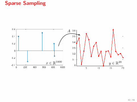
Assume that a sparsely-sampled signal y ∈ Rm (m�n) is produced by
y = Ax,
by an s-sparse vector x and a sampling matrix A. In reality, however,measurements will be noisy
y = Ax+ w.
41 / 55
Sparse Sampling
42 / 55
Sparse Sampling
We require that A satisfies the restricted isometry property[10], that is
(1− δs)‖x‖2 ≤ ‖Ax‖2 ≤ (1 + δs)‖x‖2
A typical choice is a random matrix A with entries drawn from N (0, 1m)
with m = 4s.
[10]This can be established using the Johnson-Lindenstrauss lemma.
43 / 55
Decompression
Assuming that
I w ∼ N (0, σ2I),
I the smallest element of |x| is not too small (> 8σ√
2 lnn),
I λ = 4σ√
2 lnn,
the LASSO recovers the support of x[11], that is
x? = arg min 12‖Ax− y‖
2 + λ‖x‖1,
has the same support as the actual x.
[11]Candes & Plan, 2009.
44 / 55
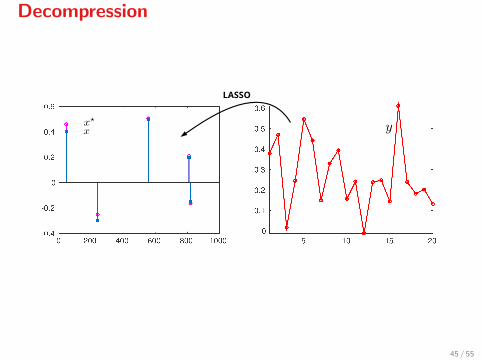
Decompression
LASSO
45 / 55
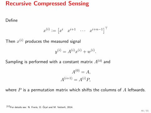
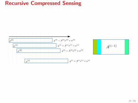
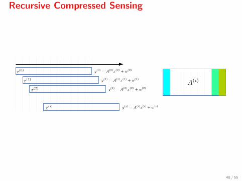
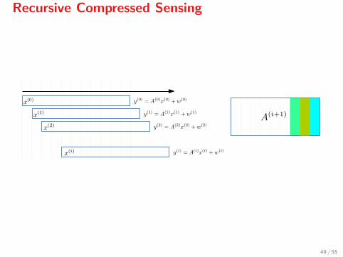
Recursive Compressed Sensing
Define
x(i) :=[xi xi+1 · · · xi+n−1
]>Then x(i) produces the measured signal
y(i) = A(i)x(i) + w(i).
Sampling is performed with a constant matrix A[12] and
A(0) = A,
A(i+1) = A(i)P,
where P is a permutation matrix which shifts the columns of A leftwards.
[12]For details see: N. Freris, O. Ocal and M. Vetterli, 2014.
46 / 55
Recursive Compressed Sensing
47 / 55
Recursive Compressed Sensing
48 / 55
Recursive Compressed Sensing
49 / 55
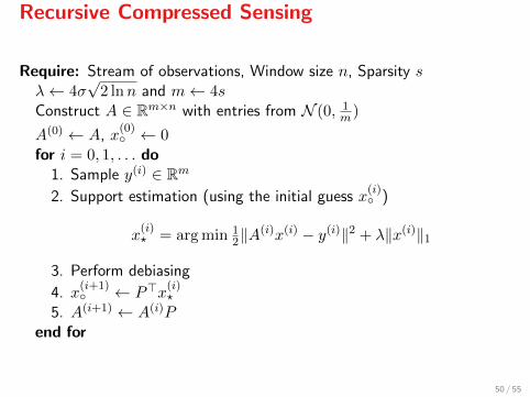
Recursive Compressed Sensing
Require: Stream of observations, Window size n, Sparsity sλ← 4σ
√2 lnn and m← 4s
Construct A ∈ Rm×n with entries from N (0, 1m)
A(0) ← A, x(0)◦ ← 0
for i = 0, 1, . . . do1. Sample y(i) ∈ Rm
2. Support estimation (using the initial guess x(i)◦ )
x(i)? = arg min 1
2‖A(i)x(i) − y(i)‖2 + λ‖x(i)‖1
3. Perform debiasing
4. x(i+1)◦ ← P>x
(i)?
5. A(i+1) ← A(i)Pend for
50 / 55
V. Simulations
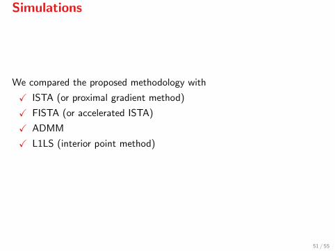
Simulations
We compared the proposed methodology with
X ISTA (or proximal gradient method)
X FISTA (or accelerated ISTA)
X ADMM
X L1LS (interior point method)
51 / 55
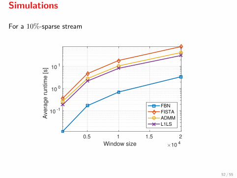
Simulations
For a 10%-sparse stream
Window size ×10 4
0.5 1 1.5 2
Avera
ge r
untim
e [s]
10 -1
10 0
10 1
FBN
FISTA
ADMM
L1LS
52 / 55
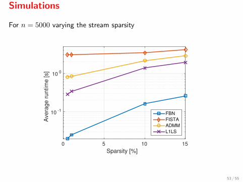
Simulations
For n = 5000 varying the stream sparsity
Sparsity [%]
0 5 10 15
Avera
ge r
untim
e [s]
10 -1
10 0
FBN
FISTA
ADMM
L1LS
53 / 55
References
1. S.-J. Kim, K. Koh, M. Lustig, S. Boyd, and D. Gorinevsky, “An interior- pointmethod for large-scale 1 -regularized least squares,” IEEE J Select Top Sign Proc,1(4), pp. 606–617, 2007.
2. A. Beck and M. Teboulle, “A fast iterative shrinkage-thresholding algo- rithm forlinear inverse problems,” SIAM J Imag Sci, 2(1), pp. 183–202, 2009.
3. S. Becker and M. J. Fadili, “A quasi-Newton proximal splitting method,” inAdvances in Neural Information Processing Systems, vol. 1, pp. 2618–2626, 2012.
4. A. Beck and M. Teboulle, “A fast iterative shrinkage-thresholding algorithm forlinear inverse problems,” SIAM J Imag Sci, 2(1), pp. 183–202, 2009.
5. P. Patrinos, L. Stella and A. Bemporad, “Forward-backward truncated Newtonmethods for convex composite optimization,” arXiv:1402.6655, 2014.
6. P. Sopasakis, N. Freris and P. Patrinos, “Accelerated reconstruction of acompressively sampled data stream,” 24th European Signal Processingconference, submitted, 2016.
7. N. Freris, O. Ocal and M. Vetterli, “Recursive Compressed Sensing,”arXiv:1312.4895, 2013.
54 / 55

Thank you for your attention.
55 / 55