Comparative testing of ellipse-fitting algorithms: implications for analysis of strain and curvature

Comparative testing of ellipse-fitting algorithms: implications for analysis

of strain and curvature

T.J. Wynna,*, S.A. Stewartb

aTRACS International, Falcon House, Union Grove Lane, Aberdeen AB10 6XU, UKbBP Azerbaijan, c/o Chertsey Road, Sunbury on Thames, Middlesex TW16 7LN, UK

Received 1 September 2004; received in revised form 26 June 2005; accepted 27 June 2005

Available online 11 August 2005

Abstract

Several types of geological problem involve fitting an ellipse to sparse data in order to define a property such as strain or curvature. The

sensitivity of ellipse-fitting algorithms to noise in input geological data is often poorly documented. Here we compare the performance of

some well-known approaches to this problem in geology against each other and an algorithm developed for machine vision. The specific

methods tested here are an analytical method, a Mohr diagram method, two least squares methods and a constrained ellipse approach. The

algorithms were tested on artificial datasets of known elliptical and noise properties. These results allow the selection of an ellipse fitting

method in a variety of geological applications and also allow an assessment of the absolute and relative accuracy of a chosen method for

various combinations of sample numbers and noise levels. For the most accurate semi axis magnitude and orientation estimates with five or

more input data, the ‘mean object’ least squares approach is recommended. However, the other least squares method also yields good results

and is also suitable for three or four data points. Where curvature data is being assessed, the least squares method is preferred as it can handle

negative principal curvature values.

q 2005 Elsevier Ltd. All rights reserved.

Keywords: Strain; Curvature; Noise; Ellipse-fitting; Least squares; Mohr-circle

1. Introduction

Determination of principal vectors, or maximum and

minimum magnitudes and directions from sparse or

scattered data, is a feature of several types of problem in

structural geology. Examples are determining two-dimen-

sional strain in classic ‘stretched belemnite’-type problems

(Lisle and Ragan, 1988 and references therein) and

estimation of principal surface curvatures (Lisle and

Robinson, 1995; Belfield, 2000). With these applications

in mind, in this paper we investigate the sensitivity of

prevailing algorithms to quality of input data.

Strain (in two dimensions) and curvature can be

represented by second order tensors (Ramsay and Huber,

1983). Tensors allow the description of the variation of a

property independently of the co-ordinate system used to

0191-8141/$ - see front matter q 2005 Elsevier Ltd. All rights reserved.

doi:10.1016/j.jsg.2005.06.010

* Corresponding author. Tel.:C44 1224 321213; fax:C44 1224 321214.

E-mail address: [email protected] (T.J. Wynn).

define the locations of the property. However, they are

linear operators that send a vector to a vector so a

description of the co-ordinate system is required for

practical purposes. In two-dimensional Cartesian space,

four components are generally required to fully define a

tensor. In the examples mentioned here, only three

components are needed since strain and surface curvature

can be represented by symmetric second order tensors with

mutually orthogonal principal axes (Ramsay and Huber,

1983; Lisle and Robinson, 1995). These properties of

symmetrical second order tensors allow them to be

represented by an ellipse, which are defined by the

magnitudes of two mutually orthogonal principal axes and

an orientation of the major axis. Strain or curvature data

usually have to be measured in directions that are likely to

be arbitrary with respect to the principal axes. Therefore, the

principal axes have to be derived from these arbitrarily

oriented measurements by fitting ellipses to the sampled

data (Lisle and Ragan, 1988; Lisle and Robinson, 1995;

Stewart and Podolski, 1998).

Many methods are available for estimating principal axes

from arbitrarily oriented measurements in geological

Journal of Structural Geology 27 (2005) 1973–1985

www.elsevier.com/locate/jsg

http://www.elsevier.com/locate/jsg

T.J. Wynn, S.A. Stewart / Journal of Structural Geology 27 (2005) 1973–19851974

situations; these methods are generally based upon

numerical ellipse fitting or an equivalent method such as

use of Mohr circles (Ramsay and Huber, 1983; Erslev and

Ge, 1990; Lisle, 1994; Lisle and Robinson, 1995; Belfield,

2000; Stewart and Wynn, 2000). However, barring a few

comments in key publications (DePaor, 1988; Robin, 2002),

there are no published indications or metrics of relative

performance of these algorithms with respect to geological

data. So, a geoscientist approaching a problem of this nature

is faced with choosing an algorithm without comparative

information. The choice is made more difficult by the fact

that several algorithms used in geological situations are

designed to give a precise answer from a restricted number

of measurements (DePaor, 1988; Lisle and Ragan, 1988),

rather than yielding a best fit from a larger number of

measurements that include some level of noise (Erslev and

Ge, 1990; McNaught, 2002). It should be noted that the

algorithms tested here all belong to the group of methods

classified as boundary based methods. These methods all

attempt to fit ellipses to a set of points that represent the

boundary of an elliptical region (Mulchrone and Choudh-

ury, 2004). An alternative group of methods are the region

based methods that use the moments of a shape to derive a

best fit ellipse that describes the shape (Hu, 1962; Teague,

1980). The advantage of region based methods is that they

are less sensitive to boundary irregularities than the

boundary based methods (Mulchrone and Choudhury,

2004). However, the purpose of this paper is to compare

the performance of algorithms within the class of boundary

based methods that are common in geological applications.

In this study we set out to test key methods against each

other using data sampled from a wide range of purpose-

built, ‘noisy’ ellipses. Rather than a detailed critique of the

theoretical merits of each algorithm, the intent of this study

was to calibrate their performance for practical application,

so that a preferred algorithm could be chosen for ellipse

estimation without a priori knowledge of dataset parameters

such as noise characteristics and principal axis orientations.

2. Ellipse fitting algorithms

Published methods previously applied to geological data

can be grouped into ‘families’ of essentially similar

approaches, namely:

(1) Analytical, or algebraic methods

(2) Mohr circle methods

(3) Least squares methods (algebraic and geometric

distances)

In this study, we chose a representative method or

methods from each group to go forward into the testing

process. The rationale behind the choice of a representative

from each ‘family’ follows, together with a more detailed

description of each selected algorithm. Within the group of

least squares methods, algebraic and geometric distances

refer to the parameters being minimised within the second

order polynomial equation representing the ellipse (see

Fitzgibbon et al. (1999) for more details). Algebraic least

squares solutions are linear and relatively simple to solve.

However, geometric fitting gives a more meaningful

parameter to minimise with respect to curved lines such as

ellipses. Unfortunately, geometric distance minimisation

methods are non-linear, requiring complex iterative sol-

utions. It should be noted that hereafter in the paper the term

‘least squares’ refers to an algebraic distance, linear least

squares minimisation. It should also be noted that all the

methods require ellipse radii and their orientations as input

and return estimates of the principal semi axes magnitudes

and orientations.

2.1. Analytical method (AN)

A number of algebraic solutions for evaluating the strain

ellipse from variously oriented longitudinal strain measure-

ments have been published (Sanderson (1977), Robin

(1983), Ragan (1987), DePaor (1988) and review by Lisle

(1994)). The approach of DePaor (1988) was selected here

because it is an exact solution and is computationally

efficient. The method was designed to yield an ‘exact’

estimate of the principal axes of strain from three reciprocal

quadratic stretches (l 0a, l0b and l 0c) in arbitrary directions,

using three simultaneous quadratic equations. First, the

angle of the major principal axis is found and this is then

used to find the principal semi axes of the ellipse. This

algorithm was published with strain analysis in mind but

other tensor data, such as curvatures, can be used instead of

stretches resulting in estimates of the principal reciprocal

quadratic curvatures. A limitation of the method is the

possibility of non-real solutions because all possible

combinations of three radii of a quadratic do not necessarily

lie on an ellipse and may be better represented by a

hyperbola (DePaor, 1988). It is also the only method to use

only three input points and is therefore not directly

comparable with the other methods tested here. However,

it is a common method and will be useful where data is very

sparse and a quick computation is required.

2.2. Mohr circle method (MC)

Mohr circle methods have been widely used in strain and

curvature problems (Means, 1982; Treagus, 1987; Lisle and

Ragan, 1988; Lisle and Robinson, 1995). The formulation

for the estimation of principal curvatures from gridded map

data described by Lisle and Robinson (1995) is adopted here

since it is designed specifically for computer implemen-

tation and deals with large digital datasets. The form of the

construction is shown in Fig. 1 and is described briefly

below for the case with four input points although the

construction is valid for more points. The reader is referred

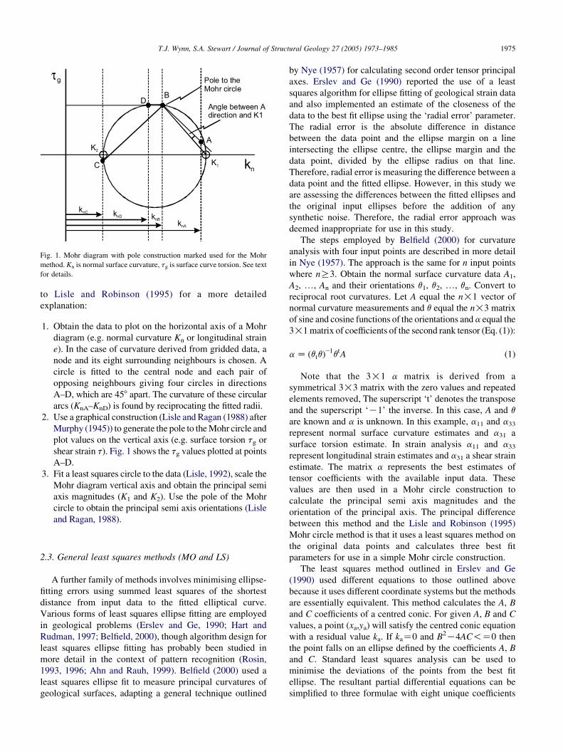
Fig. 1. Mohr diagram with pole construction marked used for the Mohr

method. Kn is normal surface curvature, tg is surface curve torsion. See text

for details.

T.J. Wynn, S.A. Stewart / Journal of Structural Geology 27 (2005) 1973–1985 1975

to Lisle and Robinson (1995) for a more detailed

explanation:

1. Obtain the data to plot on the horizontal axis of a Mohr

diagram (e.g. normal curvature Kn or longitudinal strain

e). In the case of curvature derived from gridded data, a

node and its eight surrounding neighbours is chosen. A

circle is fitted to the central node and each pair of

opposing neighbours giving four circles in directions

A–D, which are 458 apart. The curvature of these circular

arcs (KnA–KnD) is found by reciprocating the fitted radii.

2. Use a graphical construction (Lisle and Ragan (1988) after

Murphy (1945)) to generate the pole to theMohr circle and

plot values on the vertical axis (e.g. surface torsion tg or

shear strain t). Fig. 1 shows the tg values plotted at points

A–D.

3. Fit a least squares circle to the data (Lisle, 1992), scale the

Mohr diagram vertical axis and obtain the principal semi

axis magnitudes (K1 and K2). Use the pole of the Mohr

circle to obtain the principal semi axis orientations (Lisle

and Ragan, 1988).

2.3. General least squares methods (MO and LS)

A further family of methods involves minimising ellipse-

fitting errors using summed least squares of the shortest

distance from input data to the fitted elliptical curve.

Various forms of least squares ellipse fitting are employed

in geological problems (Erslev and Ge, 1990; Hart and

Rudman, 1997; Belfield, 2000), though algorithm design for

least squares ellipse fitting has probably been studied in

more detail in the context of pattern recognition (Rosin,

1993, 1996; Ahn and Rauh, 1999). Belfield (2000) used a

least squares ellipse fit to measure principal curvatures of

geological surfaces, adapting a general technique outlined

by Nye (1957) for calculating second order tensor principal

axes. Erslev and Ge (1990) reported the use of a least

squares algorithm for ellipse fitting of geological strain data

and also implemented an estimate of the closeness of the

data to the best fit ellipse using the ‘radial error’ parameter.

The radial error is the absolute difference in distance

between the data point and the ellipse margin on a line

intersecting the ellipse centre, the ellipse margin and the

data point, divided by the ellipse radius on that line.

Therefore, radial error is measuring the difference between a

data point and the fitted ellipse. However, in this study we

are assessing the differences between the fitted ellipses and

the original input ellipses before the addition of any

synthetic noise. Therefore, the radial error approach was

deemed inappropriate for use in this study.

The steps employed by Belfield (2000) for curvature

analysis with four input points are described in more detail

in Nye (1957). The approach is the same for n input points

where nR3. Obtain the normal surface curvature data A1,

A2, ., An and their orientations q1, q2, ., qn. Convert to

reciprocal root curvatures. Let A equal the n!1 vector of

normal curvature measurements and q equal the n!3 matrix

of sine and cosine functions of the orientations and a equal the

3!1matrix of coefficients of the second rank tensor (Eq. (1)):

aZ ðqtqÞK1qtA (1)

Note that the 3!1 a matrix is derived from a

symmetrical 3!3 matrix with the zero values and repeated

elements removed, The superscript ‘t’ denotes the transpose

and the superscript ‘K1’ the inverse. In this case, A and q

are known and a is unknown. In this example, a11 and a33represent normal surface curvature estimates and a31 a

surface torsion estimate. In strain analysis a11 and a33represent longitudinal strain estimates and a31 a shear strain

estimate. The matrix a represents the best estimates of

tensor coefficients with the available input data. These

values are then used in a Mohr circle construction to

calculate the principal semi axis magnitudes and the

orientation of the principal axis. The principal difference

between this method and the Lisle and Robinson (1995)

Mohr circle method is that it uses a least squares method on

the original data points and calculates three best fit

parameters for use in a simple Mohr circle construction.

The least squares method outlined in Erslev and Ge

(1990) used different equations to those outlined above

because it uses different coordinate systems but the methods

are essentially equivalent. This method calculates the A, B

and C coefficients of a centred conic. For given A, B and C

values, a point (xa,ya) will satisfy the centred conic equation

with a residual value ka. If kaZ0 and B2K4AC!Z0 then

the point falls on an ellipse defined by the coefficients A, B

and C. Standard least squares analysis can be used to

minimise the deviations of the points from the best fit

ellipse. The resultant partial differential equations can be

simplified to three formulae with eight unique coefficients


that can be rearranged to yield the centred conic equation A,

B and C values. To obtain data on the principal semi axis

orientations and magnitudes, a further three formulae are

required (see Erslev and Ge, 1990 for more details).

Throughout this text the Erslev and Ge method is referred

to as the mean object ellipse (MO) method. Strictly

speaking, the method as it is described here is a least

squares algorithm that is used as input to a mean object

ellipse technique. However, the term is used to differentiate

it from the least squares method outlined in Belfield (2000),

which is termed the least squares (LS) method in this paper.

2.4. Constrained ellipse least squares method (CE)

This method was developed by image processing

researchers as a significant refinement of least squares

ellipse fitting (Fitzgibbon et al., 1999). The method is the

first to utilise linear least squares error minimisation whilst

also constraining the fitted conic to be an ellipse. The

method was tested against other widely used approaches in

pattern recognition applications (those of Bookstein( 1979),

Taubin (1991) and Gander et al. (1994)) by Fitzgibbon et al.

(1999). These tests focused on the addition of Gaussian

noise to the data and indicated that the constrained ellipse

was the most robust approach. Based on this performance,

we selected the constrained ellipse approach for comparison

with the methods described so far. The method as presented

in Fitzgibbon et al. (1999) is described briefly below. To fit

ellipses directly whilst retaining the efficiency of a linear

least squares approach, it is required that the appropriate

constraint is always b2K4ac!0. In practice, this con-

strained problem is difficult to solve. This is circumvented

by scaling the parameters to obtain the equality constraint

4acKb2Z1. This is a quadratic constraint, which may be

expressed in matrix form. Although the minimisation only

yields one elliptical solution, Fitzgibbon et al. (1999) noted

that this ellipse is inherently biased toward low eccentricity.

Eccentricity is defined in Eq. (2):

eZ

ffiffiffiffiffiffiffiffiffiffiffiffiffi1K

b2

a2

r(2)

where 0!e!1. It should be noted that e is not used in this

study because it becomes asymptotic to 1 above axial ratios

of 10 and the testing described here used axial ratios up to

60. However, lower eccentricities correlate with lower axial

ratios.

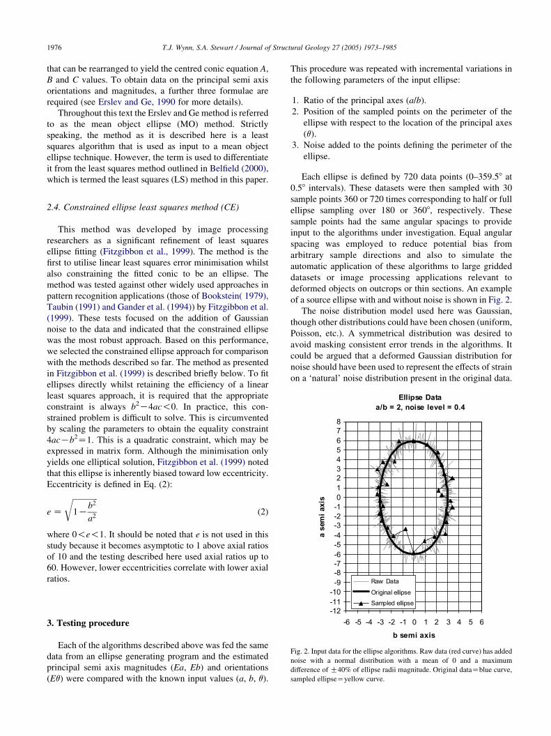
Fig. 2. Input data for the ellipse algorithms. Raw data (red curve) has added

noise with a normal distribution with a mean of 0 and a maximum

difference of G40% of ellipse radii magnitude. Original dataZblue curve,

sampled ellipseZyellow curve.

3. Testing procedure

Each of the algorithms described above was fed the same

data from an ellipse generating program and the estimated

principal semi axis magnitudes (Ea, Eb) and orientations

(Eq) were compared with the known input values (a, b, q).

This procedure was repeated with incremental variations in

the following parameters of the input ellipse:

1. Ratio of the principal axes (a/b).

2. Position of the sampled points on the perimeter of the

ellipse with respect to the location of the principal axes

(q).

3. Noise added to the points defining the perimeter of the

ellipse.

Each ellipse is defined by 720 data points (0–359.58 at

0.58 intervals). These datasets were then sampled with 30

sample points 360 or 720 times corresponding to half or full

ellipse sampling over 180 or 3608, respectively. These

sample points had the same angular spacings to provide

input to the algorithms under investigation. Equal angular

spacing was employed to reduce potential bias from

arbitrary sample directions and also to simulate the

automatic application of these algorithms to large gridded

datasets or image processing applications relevant to

deformed objects on outcrops or thin sections. An example

of a source ellipse with and without noise is shown in Fig. 2.

The noise distribution model used here was Gaussian,

though other distributions could have been chosen (uniform,

Poisson, etc.). A symmetrical distribution was desired to

avoid masking consistent error trends in the algorithms. It

could be argued that a deformed Gaussian distribution for

noise should have been used to represent the effects of strain

on a ‘natural’ noise distribution present in the original data.


However, this would only be suitable to strain measure-

ments and would also imply that no noise or error existed in

the sample measurement techniques. The source Gaussian

noise distribution used had a mean of zero and standard

deviation of G1. This initial noise distribution was then

normalised by the largest absolute value of the minimum

and maximum to beK1!n!1. This noise distribution was

then scaled again as a proportion (0.4) of the sampled ellipse

radii length. The noise was then added to the original ellipse

radii (see Fig. 2). The formula used is shown in Eq. (3):

r Z rCens (3)

where rZellipse radii, eZellipse radii length, nZGaussian

random noise with mean of 0 and range between K1 and 1

and sZnoise level scaling value of 0 or 0.4. This noise

model is static in the sense that the added noise remains the

same for each radius even when the ellipse sampling is

rotated. This has the effect of the noise distribution only

being sampled over a window width equal to 180/n or 360/n

where n is the number of sample directions. Whilst this

should be expected to produce a repeating pattern in the

results every 180/n or 360/n degrees, it does not always do

so.

It should be noted that for curvature data, one or both of

the principal curvatures can be negative. For the least

squares and Mohr circle algorithms this is not a problem as

they both utilise a Mohr circle construction that can return

negative principal semi axis magnitudes. However, the

analytical, mean object and constrained ellipse methods can

only calculate curvature where both values are positive.

4. Results

The size of the dataset output in this study precludes

exhaustive reporting here. Instead we restrict discussion of

results to key correlations and findings that might influence

choice of algorithm. Throughout this discussion, a and b are

the real major and minor ellipse semi axes (i.e. semi axis

magnitudes of noise-free source ellipse; Fig. 2) and Ea and

Eb are the corresponding estimates of major and minor semi

axis yielded by each algorithm. In this section the terms a

axis and b axis are often used on plots for conciseness but all

plots and text in this paper refer to the estimated or actual

ellipse semi axis magnitudes. Eq is the azimuth of the

estimated a semi axis relative to the vertical or y axis in the

local coordinate system (Fig. 2) and q is the angle of the

original ellipse a semi axis and the vertical or y axis. a/b is

the axial ratio of the noise free source ellipse. Axial ratios up

to 60 were examined in these experiments, since high axial

ratios are relevant in very high strain shear zones and also

represent a tendency towards cylindrical surface structures

relevant in curvature analysis. However, the principle

reason behind testing to very high axial ratios was to see

at what point the algorithm performances degraded

noticeably. The a/b axis is displayed as a log scale in

order to emphasise data in the a/b!10 range, which are

particularly relevant to strain analysis.

For the testing reported here, 30 input points were used

for all the algorithms spread over 3608. This was to ensure

full sampling of each ellipse and to avoid sampling

problems in the least squares fitting methods. The exception

to this is the analytical algorithm (DePaor, 1988), which is

designed for use with only three input data. In addition, the

Mohr circle algorithm was further tested with 30 points with

68 sample angles over 1808 because of severe problems

when using the 128 sample spacing (see below). The results

examine algorithm performance by assessing the axial ratios

of the estimated ellipses, and comparing estimates of each

semi axis with the actual semi axis magnitude with noise

levels of 0.4. Finally, the accuracy of estimated ellipse

orientation is reported. It should be noted that the ellipse

major and minor semi axis estimates for zero noise were

perfect for most algorithms within numerical rounding

errors. However, the analytical and Mohr circle methods

were susceptible to some biases and problems with zero

noise and these are discussed below.

The analytical method displayed artefacts in the Ea, Eb

and Eq results at a semi axis angles of 60, 150, 240 and 3308.

These directions correspond to the positions where the a

semi axis direction bisects two of the sample directions and

two of the three points have identical values. Therefore, the

algorithm does not have three independent input values and

cannot compute an ellipse. The Mohr circle method when

used with the 128 sample spacing produced artefacts with

zero noise levels. These appeared to worsen within certain a

semi axis angle ranges that change systematically when the

pole to the Mohr circle is changed. Fig. 3 shows the results

obtained at a and b semi axes values of 6 and 3, respectively,

using sample directions of 0 and 1808 for the pole to the

Mohr circle. The results are worse for the Ea values but the

Eb values also show perturbations. With the addition of

noise the results became unusable with many non-numeric

values for the semi axis magnitudes and Eq values clustered

around 45 and 1358. Therefore, further testing of the Mohr

circle method was undertaken using 30 input points with 68

spacing over 1808. At zero noise, this produced perfect

values of Ea and Eb, within numerical rounding errors, for

all q values. However, artefacts did occur with the addition

of noise, which are discussed below.

4.1. Ellipse axial ratio variations

Fig. 4 shows estimated vs. actual ellipse eccentricity

(Ea/Eb vs. a/b) for all the methods with noise levels of 0.4.

It can be seen that for the least squares, constrained ellipse

and mean object methods there are relatively small

underestimates or overestimates of Ea/Eb up to values of

8 and then relatively large underestimates at larger axial

ratios for the least squares and constrained ellipse methods.

The analytical and Mohr circle methods display less

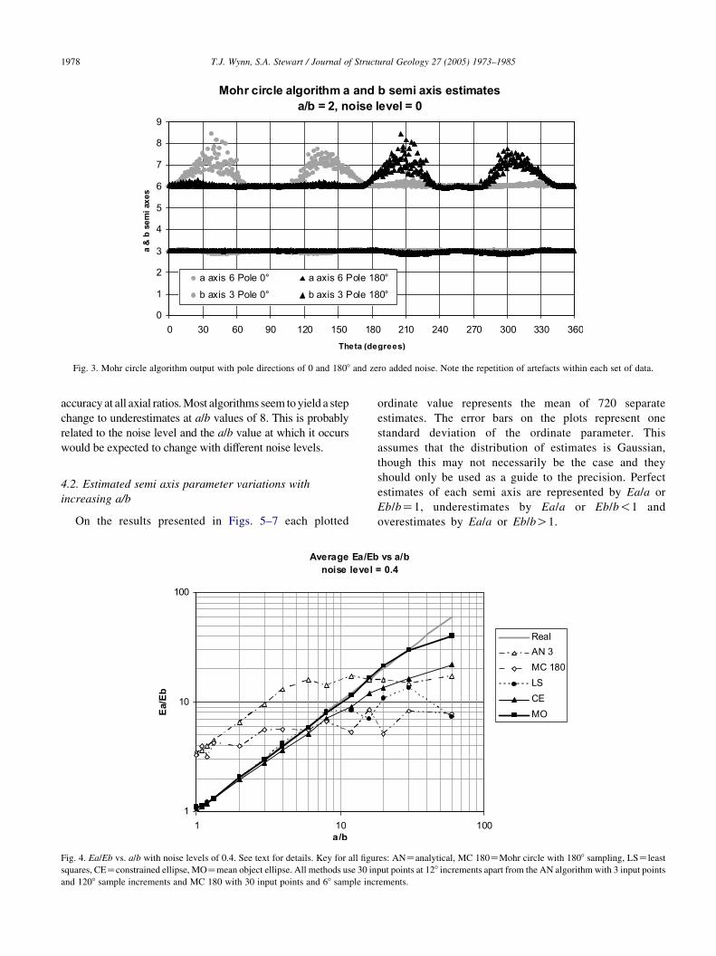
Fig. 3. Mohr circle algorithm output with pole directions of 0 and 1808 and zero added noise. Note the repetition of artefacts within each set of data.


accuracy at all axial ratios.Most algorithms seem toyield a step

change to underestimates at a/b values of 8. This is probably

related to the noise level and the a/b value at which it occurs

would be expected to change with different noise levels.

4.2. Estimated semi axis parameter variations with

increasing a/b

On the results presented in Figs. 5–7 each plotted

Fig. 4. Ea/Eb vs. a/b with noise levels of 0.4. See text for details. Key for all figu

squares, CEZconstrained ellipse, MOZmean object ellipse. All methods use 30 in

and 1208 sample increments and MC 180 with 30 input points and 68 sample inc

ordinate value represents the mean of 720 separate

estimates. The error bars on the plots represent one

standard deviation of the ordinate parameter. This

assumes that the distribution of estimates is Gaussian,

though this may not necessarily be the case and they

should only be used as a guide to the precision. Perfect

estimates of each semi axis are represented by Ea/a or

Eb/bZ1, underestimates by Ea/a or Eb/b!1 and

overestimates by Ea/a or Eb/bO1.

res: ANZanalytical, MC 180ZMohr circle with 1808 sampling, LSZleast

put points at 128 increments apart from the AN algorithm with 3 input points

rements.

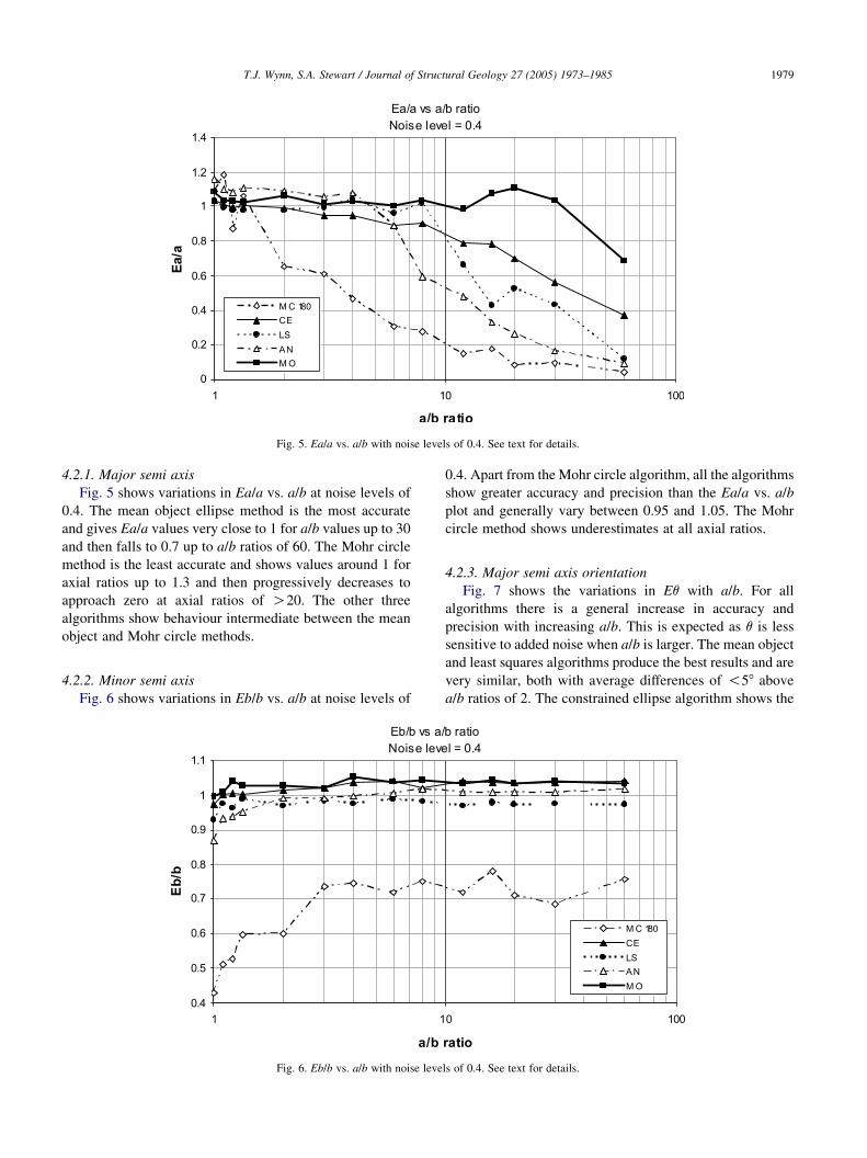
Fig. 5. Ea/a vs. a/b with noise levels of 0.4. See text for details.


4.2.1. Major semi axis

Fig. 5 shows variations in Ea/a vs. a/b at noise levels of

0.4. The mean object ellipse method is the most accurate

and gives Ea/a values very close to 1 for a/b values up to 30

and then falls to 0.7 up to a/b ratios of 60. The Mohr circle

method is the least accurate and shows values around 1 for

axial ratios up to 1.3 and then progressively decreases to

approach zero at axial ratios of O20. The other three

algorithms show behaviour intermediate between the mean

object and Mohr circle methods.

4.2.2. Minor semi axis

Fig. 6 shows variations in Eb/b vs. a/b at noise levels of

Fig. 6. Eb/b vs. a/b with noise leve

0.4. Apart from the Mohr circle algorithm, all the algorithms

show greater accuracy and precision than the Ea/a vs. a/b

plot and generally vary between 0.95 and 1.05. The Mohr

circle method shows underestimates at all axial ratios.

4.2.3. Major semi axis orientation

Fig. 7 shows the variations in Eq with a/b. For all

algorithms there is a general increase in accuracy and

precision with increasing a/b. This is expected as q is less

sensitive to added noise when a/b is larger. The mean object

and least squares algorithms produce the best results and are

very similar, both with average differences of !58 above

a/b ratios of 2. The constrained ellipse algorithm shows the

ls of 0.4. See text for details.

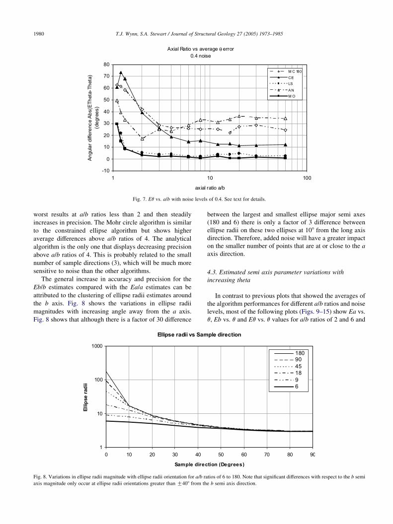
Fig. 7. Eq vs. a/b with noise levels of 0.4. See text for details.


worst results at a/b ratios less than 2 and then steadily

increases in precision. The Mohr circle algorithm is similar

to the constrained ellipse algorithm but shows higher

average differences above a/b ratios of 4. The analytical

algorithm is the only one that displays decreasing precision

above a/b ratios of 4. This is probably related to the small

number of sample directions (3), which will be much more

sensitive to noise than the other algorithms.

The general increase in accuracy and precision for the

Eb/b estimates compared with the Ea/a estimates can be

attributed to the clustering of ellipse radii estimates around

the b axis. Fig. 8 shows the variations in ellipse radii

magnitudes with increasing angle away from the a axis.

Fig. 8 shows that although there is a factor of 30 difference

Fig. 8. Variations in ellipse radii magnitude with ellipse radii orientation for a/b ra

axis magnitude only occur at ellipse radii orientations greater than G408 from th

between the largest and smallest ellipse major semi axes

(180 and 6) there is only a factor of 3 difference between

ellipse radii on these two ellipses at 108 from the long axis

direction. Therefore, added noise will have a greater impact

on the smaller number of points that are at or close to the a

axis direction.

4.3. Estimated semi axis parameter variations with

increasing theta

In contrast to previous plots that showed the averages of

the algorithm performances for different a/b ratios and noise

levels, most of the following plots (Figs. 9–15) show Ea vs.

q, Eb vs. q and Eq vs. q values for a/b ratios of 2 and 6 and

tios of 6 to 180. Note that significant differences with respect to the b semi

e b semi axis direction.

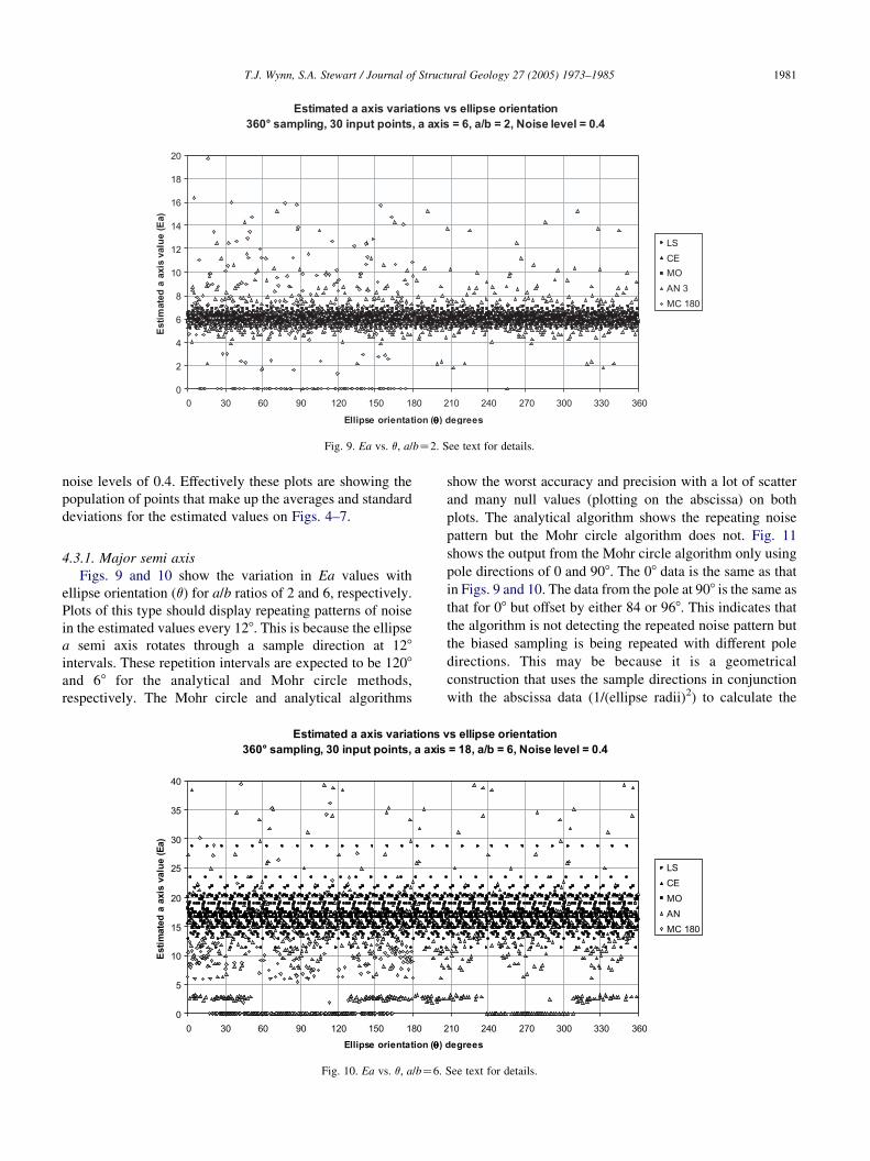
Fig. 9. Ea vs. q, a/bZ2. See text for details.


noise levels of 0.4. Effectively these plots are showing the

population of points that make up the averages and standard

deviations for the estimated values on Figs. 4–7.

4.3.1. Major semi axis

Figs. 9 and 10 show the variation in Ea values with

ellipse orientation (q) for a/b ratios of 2 and 6, respectively.

Plots of this type should display repeating patterns of noise

in the estimated values every 128. This is because the ellipse

a semi axis rotates through a sample direction at 128

intervals. These repetition intervals are expected to be 1208

and 68 for the analytical and Mohr circle methods,

respectively. The Mohr circle and analytical algorithms

Fig. 10. Ea vs. q, a/bZ6.

show the worst accuracy and precision with a lot of scatter

and many null values (plotting on the abscissa) on both

plots. The analytical algorithm shows the repeating noise

pattern but the Mohr circle algorithm does not. Fig. 11

shows the output from the Mohr circle algorithm only using

pole directions of 0 and 908. The 08 data is the same as that

in Figs. 9 and 10. The data from the pole at 908 is the same as

that for 08 but offset by either 84 or 968. This indicates that

the algorithm is not detecting the repeated noise pattern but

the biased sampling is being repeated with different pole

directions. This may be because it is a geometrical

construction that uses the sample directions in conjunction

with the abscissa data (1/(ellipse radii)2) to calculate the

See text for details.

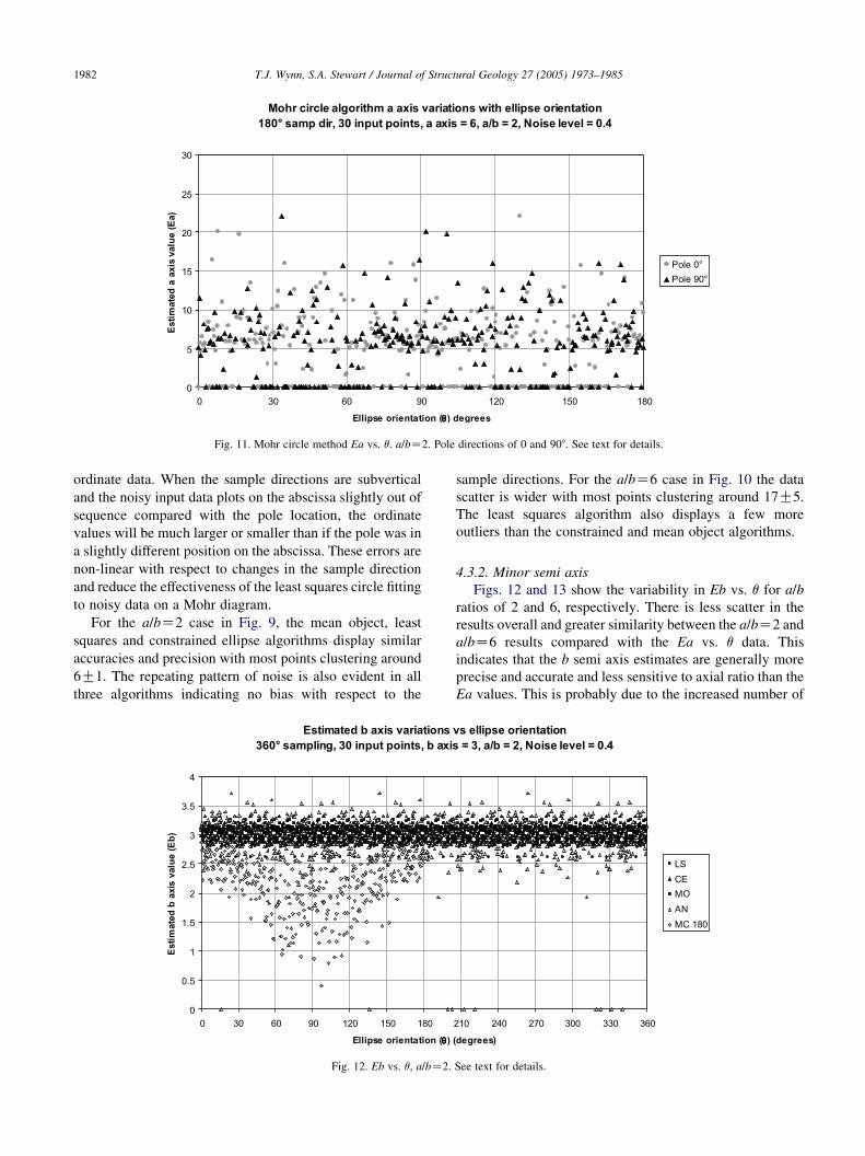
Fig. 11. Mohr circle method Ea vs. q. a/bZ2. Pole directions of 0 and 908. See text for details.


ordinate data. When the sample directions are subvertical

and the noisy input data plots on the abscissa slightly out of

sequence compared with the pole location, the ordinate

values will be much larger or smaller than if the pole was in

a slightly different position on the abscissa. These errors are

non-linear with respect to changes in the sample direction

and reduce the effectiveness of the least squares circle fitting

to noisy data on a Mohr diagram.

For the a/bZ2 case in Fig. 9, the mean object, least

squares and constrained ellipse algorithms display similar

accuracies and precision with most points clustering around

6G1. The repeating pattern of noise is also evident in all

three algorithms indicating no bias with respect to the

Fig. 12. Eb vs. q, a/bZ2.

sample directions. For the a/bZ6 case in Fig. 10 the data

scatter is wider with most points clustering around 17G5.

The least squares algorithm also displays a few more

outliers than the constrained and mean object algorithms.

4.3.2. Minor semi axis

Figs. 12 and 13 show the variability in Eb vs. q for a/b

ratios of 2 and 6, respectively. There is less scatter in the

results overall and greater similarity between the a/bZ2 and

a/bZ6 results compared with the Ea vs. q data. This

indicates that the b semi axis estimates are generally more

precise and accurate and less sensitive to axial ratio than the

Ea values. This is probably due to the increased number of


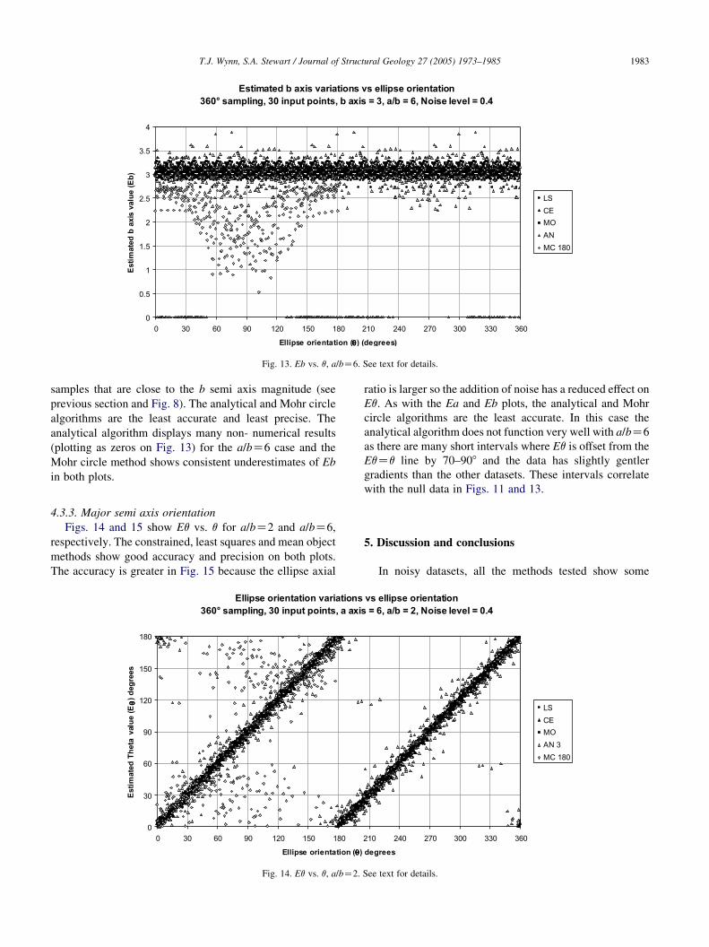
Fig. 13. Eb vs. q, a/bZ6. See text for details.


samples that are close to the b semi axis magnitude (see

previous section and Fig. 8). The analytical and Mohr circle

algorithms are the least accurate and least precise. The

analytical algorithm displays many non- numerical results

(plotting as zeros on Fig. 13) for the a/bZ6 case and the

Mohr circle method shows consistent underestimates of Eb

in both plots.

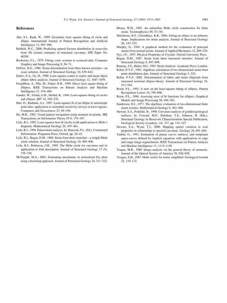
4.3.3. Major semi axis orientation

Figs. 14 and 15 show Eq vs. q for a/bZ2 and a/bZ6,

respectively. The constrained, least squares and mean object

methods show good accuracy and precision on both plots.

The accuracy is greater in Fig. 15 because the ellipse axial

Fig. 14. Eq vs. q, a/bZ2.

ratio is larger so the addition of noise has a reduced effect on

Eq. As with the Ea and Eb plots, the analytical and Mohr

circle algorithms are the least accurate. In this case the

analytical algorithm does not function very well with a/bZ6

as there are many short intervals where Eq is offset from the

EqZq line by 70–908 and the data has slightly gentler

gradients than the other datasets. These intervals correlate

with the null data in Figs. 11 and 13.

5. Discussion and conclusions

In noisy datasets, all the methods tested show some


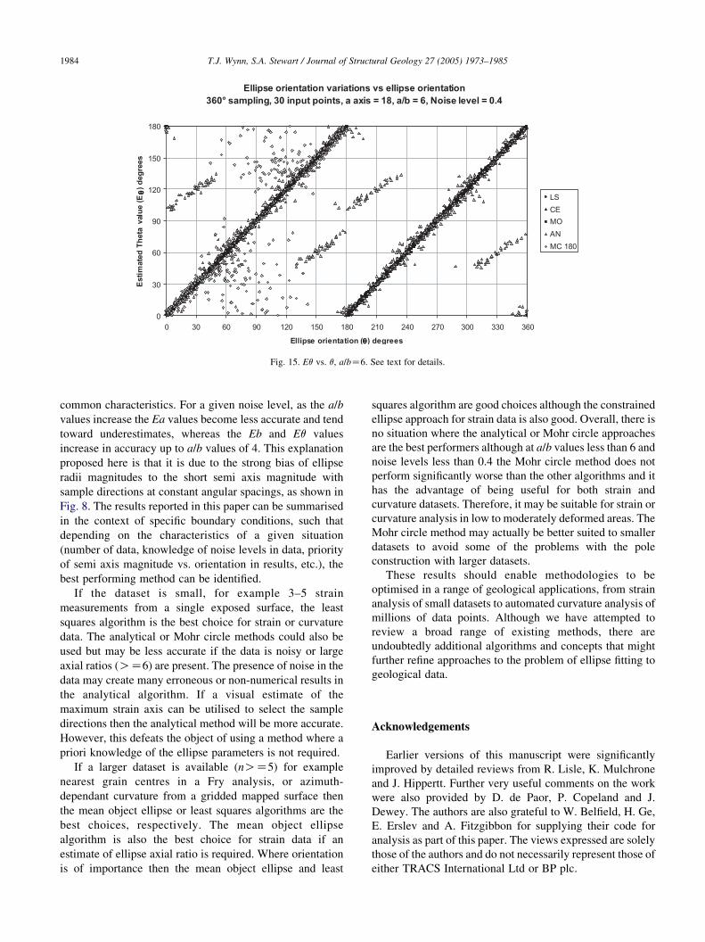
Fig. 15. Eq vs. q, a/bZ6. See text for details.


common characteristics. For a given noise level, as the a/b

values increase the Ea values become less accurate and tend

toward underestimates, whereas the Eb and Eq values

increase in accuracy up to a/b values of 4. This explanation

proposed here is that it is due to the strong bias of ellipse

radii magnitudes to the short semi axis magnitude with

sample directions at constant angular spacings, as shown in

Fig. 8. The results reported in this paper can be summarised

in the context of specific boundary conditions, such that

depending on the characteristics of a given situation

(number of data, knowledge of noise levels in data, priority

of semi axis magnitude vs. orientation in results, etc.), the

best performing method can be identified.

If the dataset is small, for example 3–5 strain

measurements from a single exposed surface, the least

squares algorithm is the best choice for strain or curvature

data. The analytical or Mohr circle methods could also be

used but may be less accurate if the data is noisy or large

axial ratios (OZ6) are present. The presence of noise in the

data may create many erroneous or non-numerical results in

the analytical algorithm. If a visual estimate of the

maximum strain axis can be utilised to select the sample

directions then the analytical method will be more accurate.

However, this defeats the object of using a method where a

priori knowledge of the ellipse parameters is not required.

If a larger dataset is available (nOZ5) for example

nearest grain centres in a Fry analysis, or azimuth-

dependant curvature from a gridded mapped surface then

the mean object ellipse or least squares algorithms are the

best choices, respectively. The mean object ellipse

algorithm is also the best choice for strain data if an

estimate of ellipse axial ratio is required. Where orientation

is of importance then the mean object ellipse and least

squares algorithm are good choices although the constrained

ellipse approach for strain data is also good. Overall, there is

no situation where the analytical or Mohr circle approaches

are the best performers although at a/b values less than 6 and

noise levels less than 0.4 the Mohr circle method does not

perform significantly worse than the other algorithms and it

has the advantage of being useful for both strain and

curvature datasets. Therefore, it may be suitable for strain or

curvature analysis in low to moderately deformed areas. The

Mohr circle method may actually be better suited to smaller

datasets to avoid some of the problems with the pole

construction with larger datasets.

These results should enable methodologies to be

optimised in a range of geological applications, from strain

analysis of small datasets to automated curvature analysis of

millions of data points. Although we have attempted to

review a broad range of existing methods, there are

undoubtedly additional algorithms and concepts that might

further refine approaches to the problem of ellipse fitting to

geological data.

Acknowledgements

Earlier versions of this manuscript were significantly

improved by detailed reviews from R. Lisle, K. Mulchrone

and J. Hippertt. Further very useful comments on the work

were also provided by D. de Paor, P. Copeland and J.

Dewey. The authors are also grateful to W. Belfield, H. Ge,

E. Erslev and A. Fitzgibbon for supplying their code for

analysis as part of this paper. The views expressed are solely

those of the authors and do not necessarily represent those of

either TRACS International Ltd or BP plc.


References

Ahn, S.J., Rauh, W., 1999. Geometric least squares fitting of circle and

ellipse. International Journal of Pattern Recognition and Artificial

Intelligence 13, 987–996.

Belfield, W.C., 2000. Predicting natural fracture distribution in reservoirs

from 3D seismic estimates of structural curvature. SPE Paper No.

60298.

Bookstein, F.L., 1979. Fitting conic sections to scattered data. Computer

Graphics and Image Processing 9, 56–71.

DePaor, D.G., 1988. Strain determination from three known stretches—an

exact solution. Journal of Structural Geology 10, 639–642.

Erslev, E.A., Ge, H., 1990. Least-squares centre-to-centre and mean object

ellipse fabric analysis. Journal of Structural Geology 12, 1047–1059.

Fitzgibbon, A., Pilu, M., Fisher, R.B., 1999. Direct least square fitting of

ellipses. IEEE Transactions on Pattern Analysis and Machine

Intelligence 21, 476–480.

Gander, W., Golub, G.H., Strebel, R., 1994. Least-squares fitting of circles

and ellipses. BIT 34, 558–578.

Hart, D., Rudman, A.J., 1997. Least-squares fit of an ellipse to anisotropic

polar data: application to azimuthal resistivity surveys in karst regions.

Computers and Geosciences 23, 89–194.

Hu, M.K., 1962. Visual pattern recognition using moment invariants. IRE

Transactions on Information Theory IT-8, 179–187.

Lisle, R.J., 1992. Least-squares best-fit circles (with applications to Mohr’s

diagram). Mathematical Geology 24, 455–461.

Lisle, R.J., 1994. Palaeostrain analysis. In: Hancock, P.L. (Ed.), Continental

Deformation. Pergamon Press, Oxford, pp. 28–42.

Lisle, R.J., Ragan, D.M., 1988. Strain from three stretches—a simple Mohr

circle solution. Journal of Structural Geology 10, 905–906.

Lisle, R.J., Robinson, J.M., 1995. The Mohr circle for curvature and its

application to fold description. Journal of Structural Geology 17 (5),

739–750.

McNaught, M.A., 2002. Estimating uncertainty in normalized Fry plots

using a bootstrap approach. Journal of Structural Geology 24, 311–322.

Means, W.D., 1982. An unfamiliar Mohr circle construction for finite

strain. Tectonophysics 89, T1–T6.

Mulchrone, K.F., Choudhury, K.R., 2004. Fitting an ellipse to an arbitrary

shape. Implications for strain analysis. Journal of Structural Geology

26, 143–153.

Murphy, G., 1945. A graphical method for the evaluation of principal

strains from normal strains. Journal of Applied Mechanics 12, 209–210.

Nye, J.F., 1957. Physical Properties of Crystals. Oxford University Press.

Ragan, D.M., 1987. Strain from three measured stretches. Journal of

Structural Geology 9, 897–898.

Ramsay, J.G., Huber, M.I., 1983. Strain Analysis. Academic Press, London.

Robin, P-Y.F., 1983. Algebraic calculation of two dimensional strain from

point distribution data. Journal of Structural Geology 5, 552.

Robin, P-Y.F., 2002. Determination of fabric and strain ellipsoids from

measured sectional ellipses-theory. Journal of Structural Geology 24,

513–544.

Rosin, P.L., 1993. A note on the least-squares fitting of ellipses. Pattern

Recognition Letters 14, 799–808.

Rosin, P.L., 1996. Assessing error of fit functions for ellipses. Graphical

Models and Image Processing 58, 494–502.

Sanderson, D.J., 1977. The algebraic evaluation of two-dimensional finite

strain rosettes. Mathematical Geology 9, 483–496.

Stewart, S.A., Podolski, R., 1998. Curvature analysis of gridded geological

surfaces. In: Coward, M.P., Daltaban, T.S., Johnson, H. (Eds.),

Structural Geology in Reservoir Characterisation Special Publication,

Geological Society (London), vol. 127, pp. 133–147.

Stewart, S.A., Wynn, T.J., 2000. Mapping spatial variation in rock

properties in relationship to spectral curvature. Geology 28, 691–694.

Taubin, G., 1991. Estimation of planar curves surfaces, and nonplanar

space-curves defined by implicit equations with applications to edge

and range image segmentation. IEEE Transactions on Pattern Analysis

and Machine Intelligence 13, 1115–1138.

Teague, M.R., 1980. Image analysis via the general theory of moments.

Journal of the Optical Society of America 70, 920–930.

Treagus, S.H., 1987. Mohr circles for strain, simplified. Geological Journal

22, 119–132.

Documents

Comparative testing of ellipse-fitting algorithms: implications for analysis of strain and curvature