1 University of Parma, ITALY1 Rieter Automotive Systems,

Switzerland

Angelo Farina1, Fabio Bozzoli1, Patricia Strasser2

Comparative Study of Speech Intelligibility Inside Cars

2

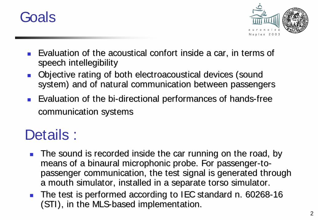
Goals

Evaluation of the acoustical Evaluation of the acoustical confortconfort inside a car, in terms of inside a car, in terms of speech speech intellegibilityintellegibilityObjective rating of both Objective rating of both electroacousticalelectroacoustical devices (sound devices (sound system) and of natural communication between passengers system) and of natural communication between passengers

Evaluation of the biEvaluation of the bi--directional performances of handsdirectional performances of hands--free free communication systems communication systems

Details :The sound is recorded inside the car running on the road, by The sound is recorded inside the car running on the road, by means of a binaural means of a binaural microphonicmicrophonic probe. For passengerprobe. For passenger--toto--passenger communication, the test signal is generated through passenger communication, the test signal is generated through a mouth simulator, installed in a separate torso simulator.a mouth simulator, installed in a separate torso simulator.The test is performed according to IEC standard n. 60268The test is performed according to IEC standard n. 60268--16 16 (STI), in the MLS(STI), in the MLS--based implementation.based implementation.

3

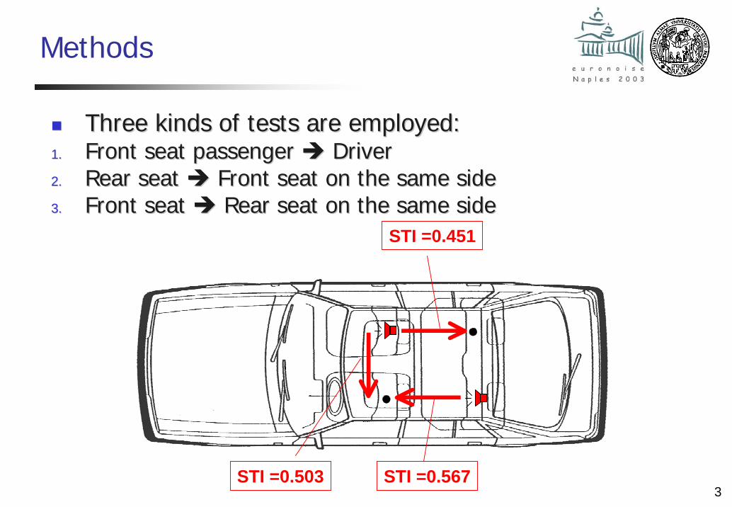
Methods

Three kinds of tests are employed: Three kinds of tests are employed: 1.1. Front seat passenger Front seat passenger Driver Driver 2.2. Rear seat Rear seat Front seat on the same sideFront seat on the same side3.3. Front seat Front seat Rear seat on the same sideRear seat on the same side

STI =0.567

STI =0.451

STI =0.503

4

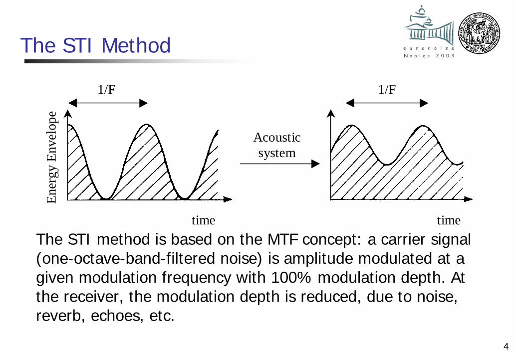
The STI Method

The STI method is based on the MTF concept: a carrier signal (one-octave-band-filtered noise) is amplitude modulated at a given modulation frequency with 100% modulation depth. At the receiver, the modulation depth is reduced, due to noise, reverb, echoes, etc.

Ener

gy E

nvel

ope

Acousticsystem

1/F 1/F

time time

5

MTF from Impulse Response

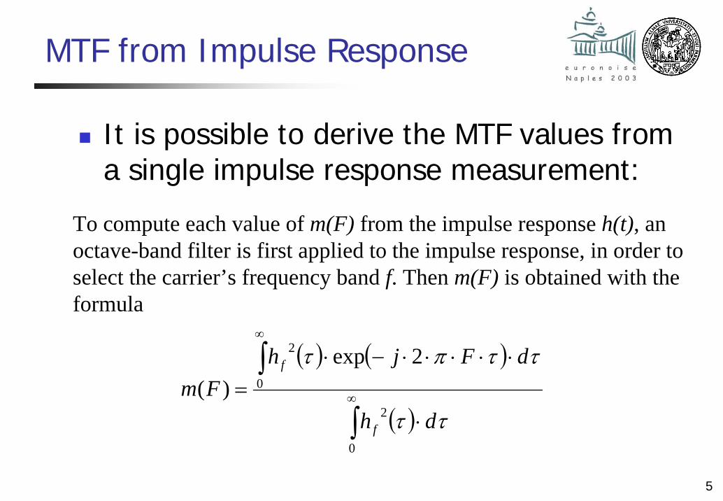
It is possible to derive the MTF values from a single impulse response measurement:

( ) ( )

( )∫

∫∞

∞

⋅

⋅⋅⋅⋅⋅−⋅=

0

2

0

2 2exp)(

ττ

ττπτ

dh

dFjhFm

f

f

To compute each value of m(F) from the impulse response h(t), an octave-band filter is first applied to the impulse response, in order to select the carrier’s frequency band f. Then m(F) is obtained with the formula

6

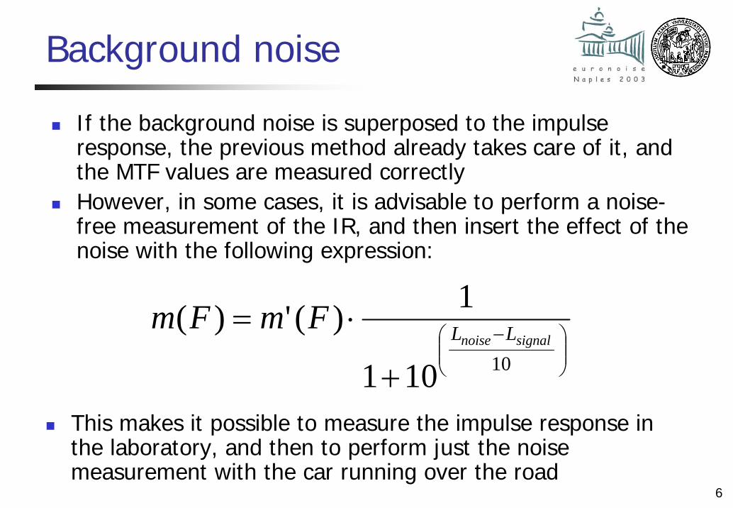
Background noise

If the background noise is superposed to the impulse response, the previous method already takes care of it, and the MTF values are measured correctlyHowever, in some cases, it is advisable to perform a noise-free measurement of the IR, and then insert the effect of the noise with the following expression:

⎟⎟⎠

⎞⎜⎜⎝

⎛ −

+

⋅=10101

1)(')(signalnoise LLFmFm

This makes it possible to measure the impulse response in the laboratory, and then to perform just the noise measurement with the car running over the road

7

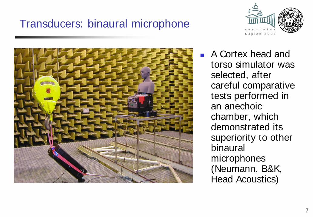
Transducers: binaural microphone

A Cortex head and torso simulator was selected, after careful comparative tests performed in an anechoic chamber, which demonstrated its superiority to other binaural microphones (Neumann, B&K, Head Acoustics)

8

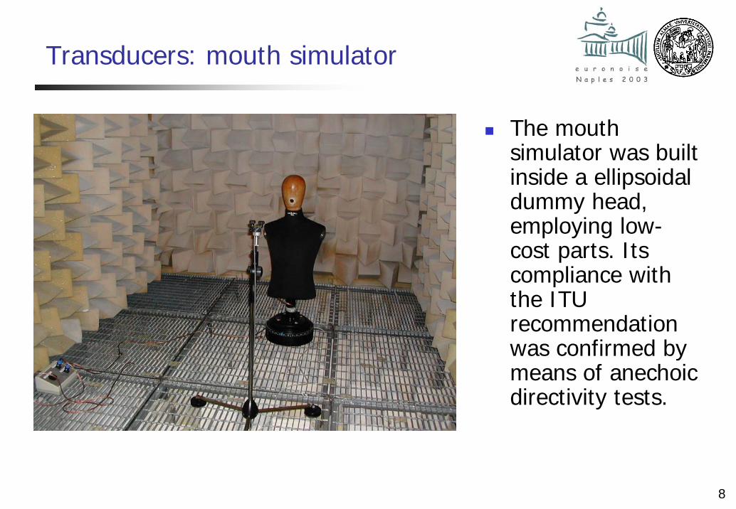
Transducers: mouth simulator

The mouth simulator was built inside a ellipsoidal dummy head, employing low-cost parts. Its compliance with the ITU recommendation was confirmed by means of anechoic directivity tests.

9

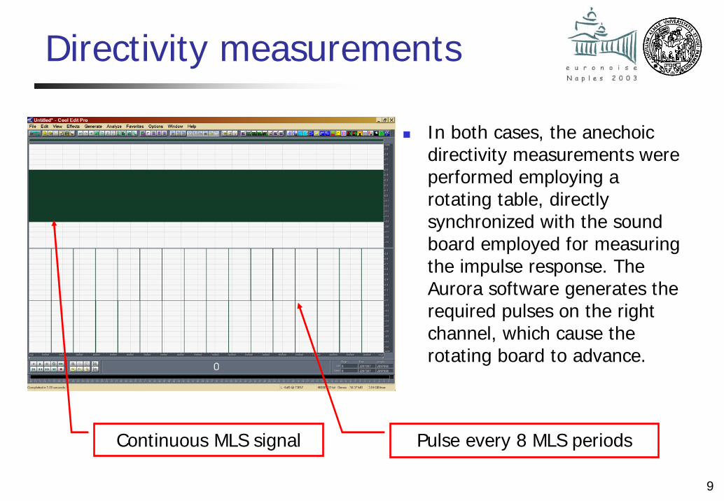
Directivity measurements

In both cases, the anechoic directivity measurements were performed employing a rotating table, directly synchronized with the sound board employed for measuring the impulse response. The Aurora software generates the required pulses on the right channel, which cause the rotating board to advance.

Continuous MLS signal Pulse every 8 MLS periods

10

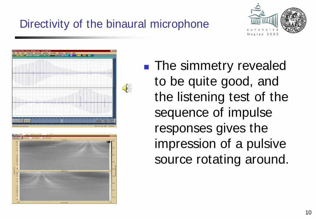
Directivity of the binaural microphone

The simmetry revealed to be quite good, and the listening test of the sequence of impulse responses gives the impression of a pulsivesource rotating around.

11

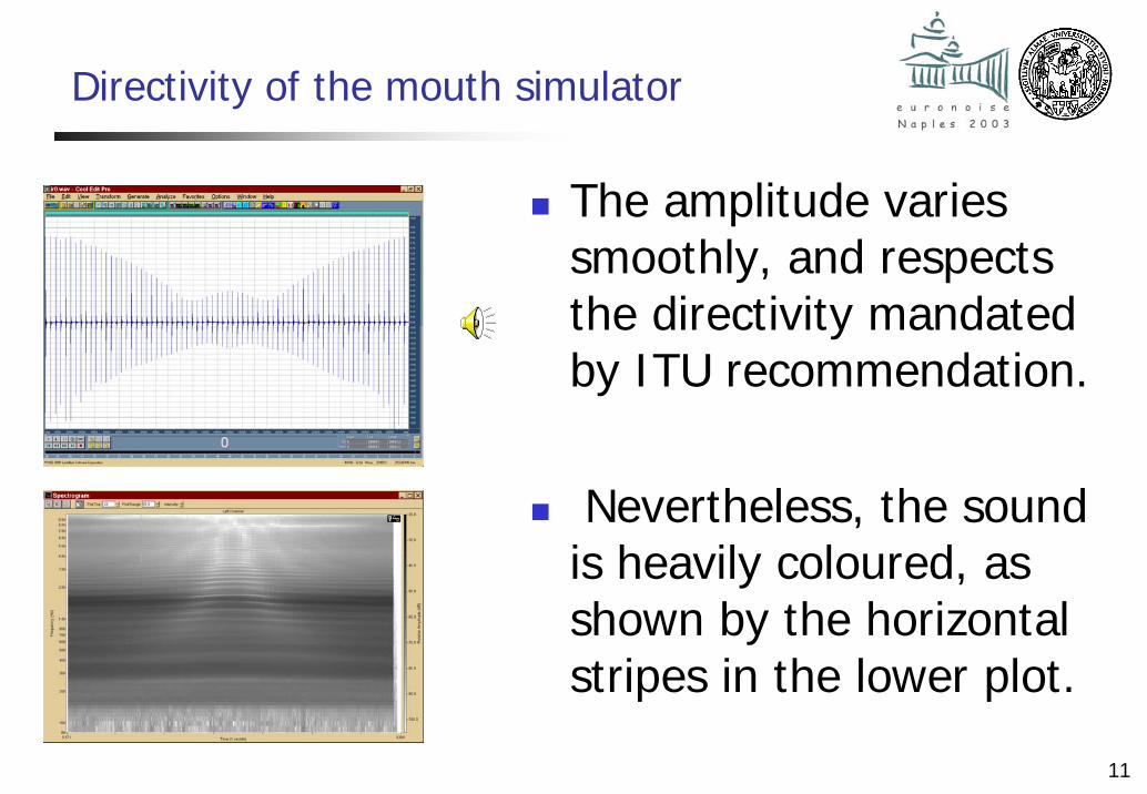
Directivity of the mouth simulator

The amplitude varies smoothly, and respects the directivity mandated by ITU recommendation.

Nevertheless, the sound is heavily coloured, as shown by the horizontal stripes in the lower plot.

12

125 Hz

-35

-25

-15

-5

5+0°

+15°+30°

+45°

+60°

+75°

+90°

+105°

+120°

+135°

+150°+165°

±180°-165°

-150°

-135°

-120°

-105°

-90°

-75°

-60°

-45°

-30°-15°

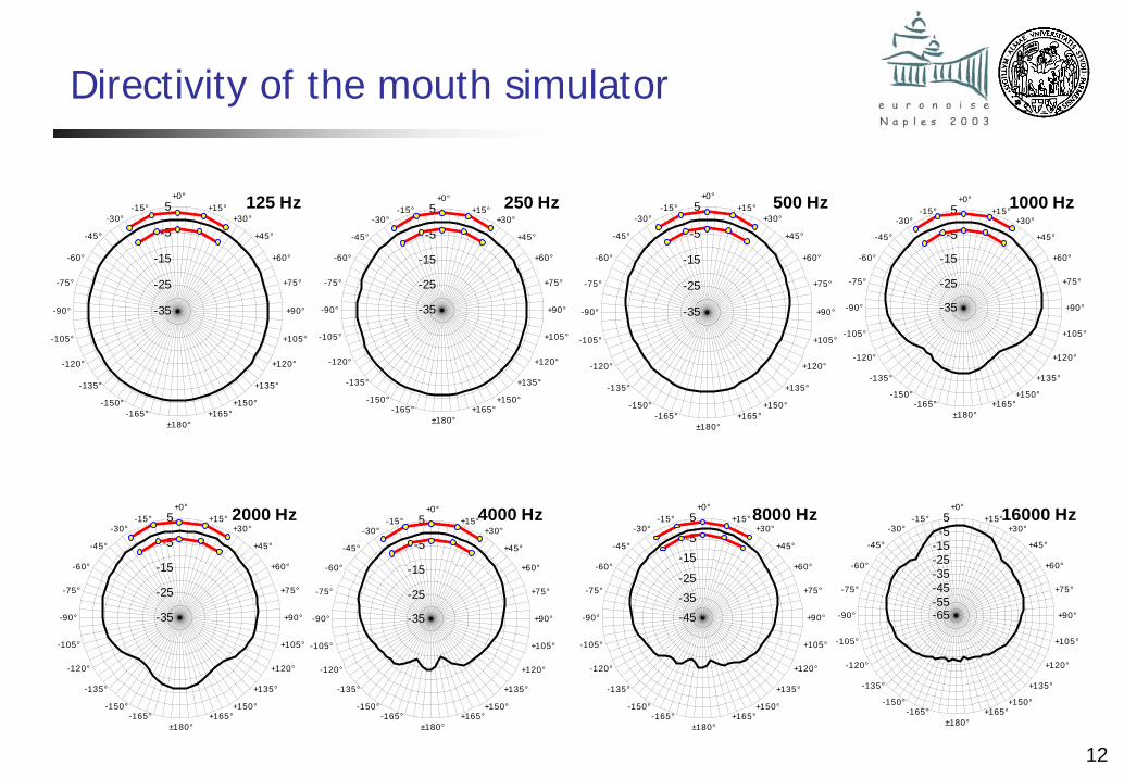
Directivity of the mouth simulator

250 Hz

-35

-25

-15

-5

5+0°

+15°+30°

+45°

+60°

+75°

+90°

+105°

+120°

+135°

+150°+165°

±180°-165°

-150°

-135°

-120°

-105°

-90°

-75°

-60°

-45°

-30°-15° 500 Hz

-35

-25

-15

-5

5+0°

+15°+30°

+45°

+60°

+75°

+90°

+105°

+120°

+135°

+150°+165°

±180°-165°

-150°

-135°

-120°

-105°

-90°

-75°

-60°

-45°

-30°-15° 1000 Hz

-35

-25

-15

-5

5+0°

+15°+30°

+45°

+60°

+75°

+90°

+105°

+120°

+135°

+150°+165°

±180°-165°

-150°

-135°

-120°

-105°

-90°

-75°

-60°

-45°

-30°-15°

2000 Hz

-35

-25

-15

-5

5+0°

+15°+30°

+45°

+60°

+75°

+90°

+105°

+120°

+135°

+150°+165°

±180°-165°

-150°

-135°

-120°

-105°

-90°

-75°

-60°

-45°

-30°-15° 4000 Hz

-35

-25

-15

-5

5+0°

+15°+30°

+45°

+60°

+75°

+90°

+105°

+120°

+135°

+150°+165°

±180°-165°

-150°

-135°

-120°

-105°

-90°

-75°

-60°

-45°

-30°-15° 8000 Hz

-45-35-25

-15-5

5+0°

+15°+30°

+45°

+60°

+75°

+90°

+105°

+120°

+135°

+150°+165°

±180°-165°

-150°

-135°

-120°

-105°

-90°

-75°

-60°

-45°

-30°-15° 16000 Hz

-65-55-45-35-25-15-55

+0°+15°

+30°

+45°

+60°

+75°

+90°

+105°

+120°

+135°

+150°+165°

±180°-165°

-150°

-135°

-120°

-105°

-90°

-75°

-60°

-45°

-30°-15°

13

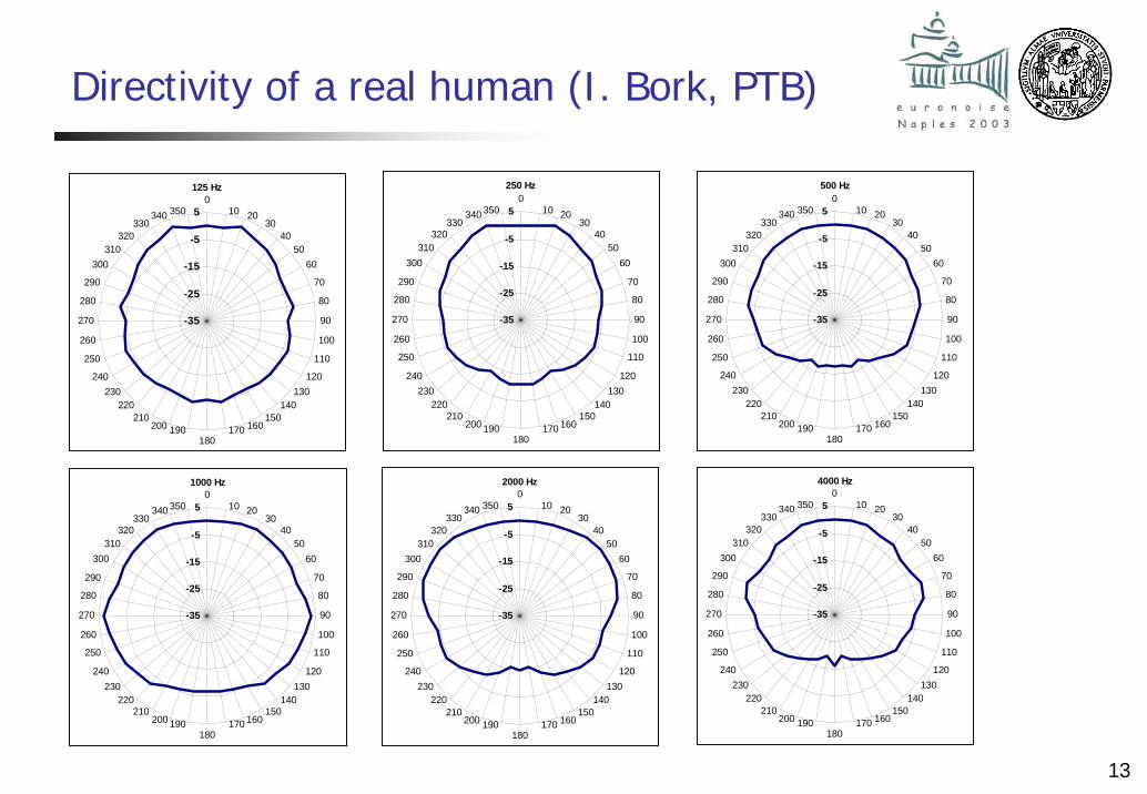
Directivity of a real human (I. Bork, PTB)

125 Hz

-35

-25

-15

-5

50

10 2030

4050

60

70

80

90

100

110

120130

140150

160170180

190200210

220230

240

250

260

270

280

290

300310

320330

340 350

250 Hz

-35

-25

-15

-5

50

10 2030

4050

60

70

80

90

100

110

120130

140150

160170180

190200210

220230

240

250

260

270

280

290

300310

320330

340 350

500 Hz

-35

-25

-15

-5

50

10 2030

4050

60

70

80

90

100

110

120130

140150

160170180

190200210

220230

240

250

260

270

280

290

300310

320330

340 350

1000 Hz

-35

-25

-15

-5

50

10 2030

4050

60

70

80

90

100

110

120130

140150

160170180

190200210

220230

240

250

260

270

280

290

300310

320330

340 350

2000 Hz

-35

-25

-15

-5

50

10 2030

4050

60

70

80

90

100

110

120130

140150

160170180

190200210

220230

240

250

260

270

280

290

300310

320330

340 350

4000 Hz

-35

-25

-15

-5

50

10 2030

4050

60

70

80

90

100

110

120130

140150

160170180

190200210

220230

240

250

260

270

280

290

300310

320330

340 350

14

Frequency responses

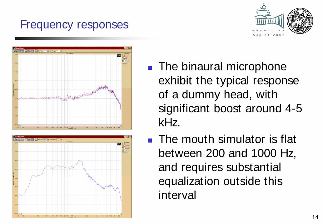
The binaural microphone exhibit the typical response of a dummy head, with significant boost around 4-5 kHz.The mouth simulator is flat between 200 and 1000 Hz, and requires substantial equalization outside this interval

15

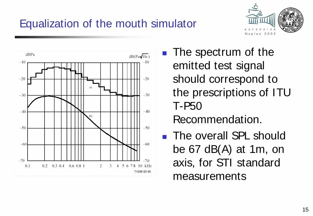
Equalization of the mouth simulator

The spectrum of the emitted test signal should correspond to the prescriptions of ITU T-P50 Recommendation.The overall SPL should be 67 dB(A) at 1m, on axis, for STI standard measurements

16

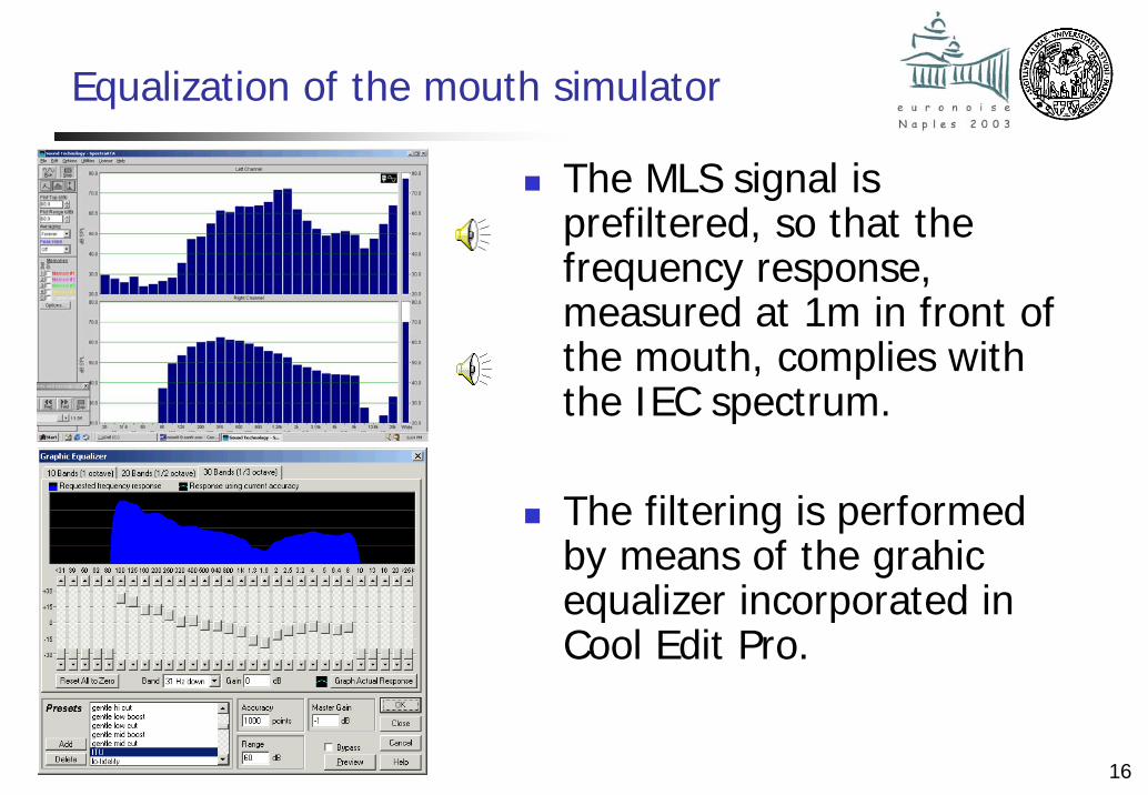
Equalization of the mouth simulator

The MLS signal is prefiltered, so that the frequency response, measured at 1m in front of the mouth, complies with the IEC spectrum.

The filtering is performed by means of the grahicequalizer incorporated in Cool Edit Pro.

17

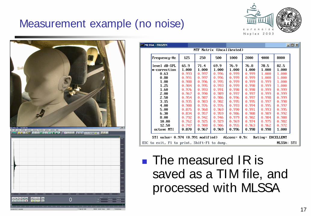
Measurement example (no noise)

The measured IR is saved as a TIM file, and processed with MLSSA

18

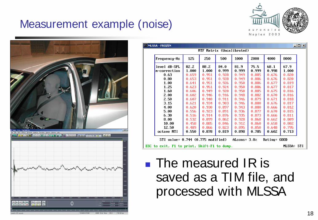
Measurement example (noise)

The measured IR is saved as a TIM file, and processed with MLSSA

19

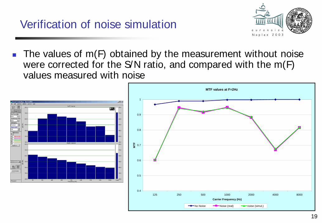
Verification of noise simulation

The values of m(F) obtained by the measurement without noise were corrected for the S/N ratio, and compared with the m(F) values measured with noise

MTF values at F=2Hz

0.4

0.5

0.6

0.7

0.8

0.9

1

125 250 500 1000 2000 4000 8000

Carrier Frequency (Hz)

MTF

No Noise Noise (real) noise (simul.)

20

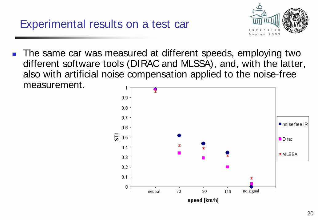
Experimental results on a test car

The same car was measured at different speeds, employing two different software tools (DIRAC and MLSSA), and, with the latter, also with artificial noise compensation applied to the noise-free measurement.

neutral 70 90 110 no signal

21

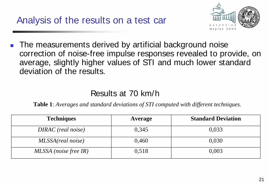
Analysis of the results on a test car

The measurements derived by artificial background noise correction of noise-free impulse responses revealed to provide, on average, slightly higher values of STI and much lower standard deviation of the results.

Table 1: Averages and standard deviations of STI computed with different techniques.

Techniques Average Standard Deviation

DIRAC (real noise) 0,345 0,033

MLSSA(real noise) 0,460 0,030

MLSSA (noise free IR) 0,518 0,003

Results at 70 km/h

22

Conclusions

The hardware and software developed allows for quick and reliable measurement of STI in cars.The background noise can be present during the actual measurement: however, it is possible to add its effect later, in two different ways:

Mixing a noise recording over the re-recorded MLS signal, prior of IR deconvolution (yet to be assessed)Correcting the MTF values with the theoretical relationship, knowing the levels of the signal and of the noise (ideal method when only the noise spectral values are known, and no recording is available)

The methodology developed, however, allows also for the creation of sound samples, containing speech (convolved with the noiseless IR) and background noise: these sound samples can be employed for listening tests.