Comparative analyses of expected shortfall · PDF file216 Comparative analyses of expected shortfall and value-at-risk under market stress1 Yasuhiro Yamai and Toshinao Yoshiba, Bank

216

Comparative analyses of expected shortfall and value-at-risk under market stress1

Yasuhiro Yamai and Toshinao Yoshiba, Bank of Japan

Abstract

In this paper, we compare value-at-risk (VaR) and expected shortfall under market stress. Assuming that the multivariate extreme value distribution represents asset returns under market stress, we simulate asset returns with this distribution. With these simulated asset returns, we examine whether market stress affects the properties of VaR and expected shortfall.

Our findings are as follows. First, VaR and expected shortfall may underestimate the risk of securities with fat-tailed properties and a high potential for large losses. Second, VaR and expected shortfall may both disregard the tail dependence of asset returns. Third, expected shortfall has less of a problem in disregarding the fat tails and the tail dependence than VaR does.

1. Introduction

It is a well known fact that value-at-risk2 (VaR) models do not work under market stress. VaR models are usually based on normal asset returns and do not work under extreme price fluctuations. The case in point is the financial market crisis of autumn 1998. Concerning this crisis, CGFS (1999) notes that �a large majority of interviewees admitted that last autumn�s events were in the �tails� of distributions and that VaR models were useless for measuring and monitoring market risk�. Our question is this: Is this a problem of the estimation methods, or of VaR as a risk measure?

The estimation methods used for standard VaR models have problems for measuring extreme price movements. They assume that the asset returns follow a normal distribution. So they disregard the fat-tailed properties of actual returns, and underestimate the likelihood of extreme price movements.

On the other hand, the concept of VaR as a risk measure has problems for measuring extreme price movements. By definition, VaR only measures the distribution quantile, and disregards extreme loss beyond the VaR level. Thus, VaR may ignore important information regarding the tails of the underlying distributions. CGFS (2000) identifies this problem as tail risk.

To alleviate the problems inherent in VaR, Artzner et al (1997, 1999) propose the use of expected shortfall. Expected shortfall is the conditional expectation of loss given that the loss is beyond the VaR level. 3 Thus, by definition, expected shortfall considers loss beyond the VaR level. Yamai and Yoshiba (2002c) show that expected shortfall has no tail risk under more lenient conditions than VaR.

1 The views expressed here are those of the authors and do not reflect those of the Bank of Japan. (E-mail:

[email protected]; [email protected].) This paper is a revised version of the paper presented at the Third Joint Central Bank Research Conference on Risk Measurement and Systemic Risk on 7-8 March 2002 in Basel. The content of this paper is the same as Yamai, Y and T Yoshiba, �Comparative analyses of expected shortfall and value-at-risk (3): their validity under market stress�, IMES Discussion Paper No 2002-E-2, Bank of Japan, 2002.

2 VaR at the 100(1-α)% confidence level is the upper 100α percentile of the loss distribution. We denote the VaR at the 100(1�α)% confidence level as VaRα(Z), where Z is the random variable of loss.

3 When the distributions of loss Z are continuous, expected shortfall at the 100(1�α)% confidence level (ESα(Z)) is defined by the following equation:

])([)( ZVaRZZEZES��

�� .

217

The existing research implies that the tail risk of VaR and expected shortfall may be more significant under market stress than under normal market conditions. The loss under market stress is larger and less frequent than that under normal conditions. According to Yamai and Yoshiba (2002a), the tail risk is significant when asset losses are infrequent and large.4

In this paper, we examine whether the tail risk of VaR and expected shortfall is actually significant under market stress. We assume that the multivariate extreme value distributions represent the asset returns under market stress. With this assumption, we simulate asset returns with those distributions, and compare VaR and expected shortfall.5,6

Our assumption of the multivariate extreme value distributions is based on the theoretical results of extreme value theory. This theory states that the multivariate exceedances over a high threshold asymptotically follow the multivariate extreme value distributions. As extremely large fluctuations characterise asset returns under market stress, we assume that the asset returns under market stress follow the multivariate extreme value distributions.

Following this Introduction, Section 2 introduces the concepts and definitions of the tail risk of VaR and expected shortfall based on Yamai and Yoshiba (2002a, 2002c). Section 3 provides a general introduction to multivariate extreme value theory. Section 4 adopts univariate extreme value distributions to examine how the fat-tailed properties of these distributions result in the problems of VaR and expected shortfall. Section 5 adopts simulations with multivariate extreme value distributions7 to examine how tail dependence results in the tail risk of VaR and expected shortfall. Section 6 presents empirical analyses to examine whether past financial crisis have resulted in the tail risk of VaR and expected shortfall. Finally, Section 7 presents the conclusions and implications of this paper.

2. Tail risk of VaR and expected shortfall

A. The definition and concept of the tail risk of VaR In this paper, we say that VaR has tail risk when VaR fails to summarise the relative choice between portfolios as a result of its underestimation of the risk of portfolios with fat-tailed properties and a high potential for large losses.8,9 The tail risk of VaR emerges since it measures only a single quantile of the profit/loss distributions and disregards any loss beyond the VaR level. This may lead one to think that securities with a higher potential for large losses are less risky than securities with a lower potential for large losses.

For example, suppose that the VaR at the 99% confidence level of portfolio A is 10 million and that of portfolio B is 15 million. Given these numbers, one may conclude that portfolio B is more risky than portfolio A. However, the investor does not know how much may be lost outside of the confidence

When the underlying distributions are discontinuous, see Definition 2 of Acerbi and Tasche (2001). 4 Jorion (2000) makes the following comment in analysing the failure of Long-Term Capital Management (LTCM): �The payoff

patterns of the investment strategy [of LTCM] were akin to short positions in options. Even if it had measured its risk correctly, the firm failed to manage its risk properly.�

5 Prior comparative analyses of VaR and expected shortfall focus on their sub-additivity. For example, Artzner et al (1997, 1999) show that expected shortfall is sub-additive, while VaR is not. Acerbi et al (2001) prove that expected shortfall is sub-additive, including the cases where the underlying profit/loss distributions are discontinuous. Rockafeller and Uryasev (2000) utilise the sub-additivity of the expected shortfall to find an efficient algorithm for optimising expected shortfall.

6 The other important aspect of the comparative analyses of VaR and expected shortfall is their estimation errors. Yamai and Yoshiba (2002b) show that expected shortfall needs a larger size sample than VaR for the same level of accuracy.

7 For other financial applications of multivariate extreme value theory, see Longin and Solnik (2001), Embrechts et al (2000) and Hartmann et al (2000).

8 We only consider whether VaR and expected shortfall are effective for the relative choice of portfolios. We do not consider the issue of the absolute level of risk, such as whether VaR is appropriate as a benchmark of risk capital.

9 For details regarding the general concept and definition of the tail risk of risk measures, see Yamai and Yoshiba (2002c).

218

interval. When the maximum loss of portfolio A is 1 trillion and that of B is 16 million, portfolio A should be considered more risky since it loses much more than portfolio B under the worst case. In this case, VaR has tail risk since VaR fails to summarise the choice between portfolios A and B as a result of its disregard of the tail of profit/loss distributions.

We further illustrate the concept of the tail risk of VaR with two examples.

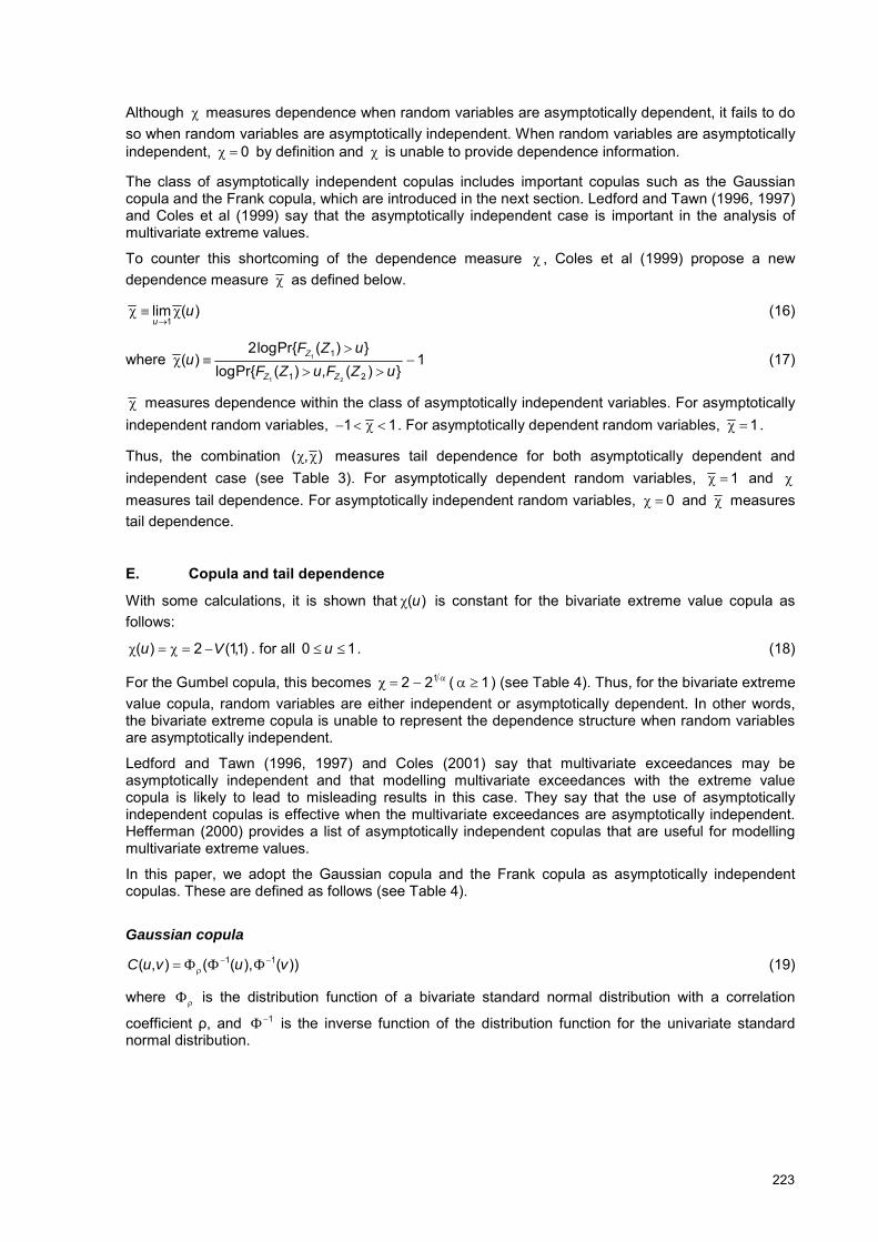
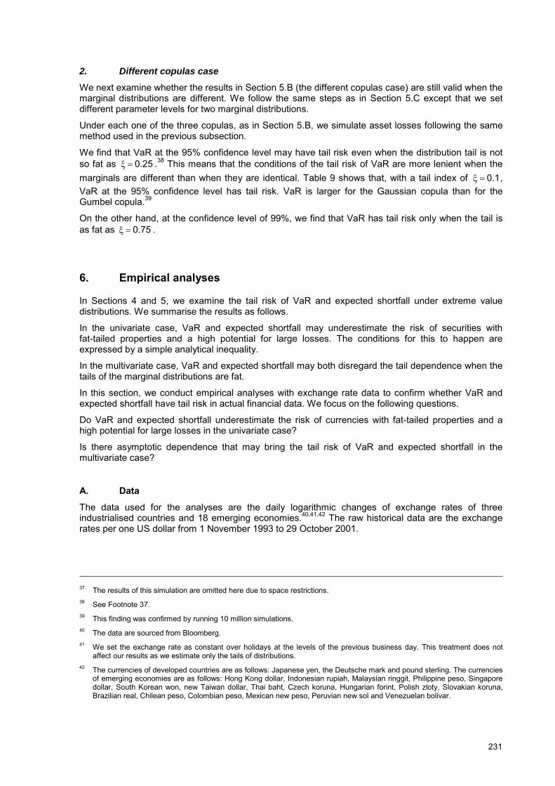
Example 1: Option portfolio (Danielsson (2001))

Danielsson (2001) shows that VaR is conducive to manipulation since it measures only a single quantile. We introduce his illustration as a typical example of the tail risk of VaR.

The solid line in Figure 1 depicts the distribution function of the profit/loss of a given security. The VaR of this security is VaR0 as it is the lower quantile of the profit/loss distribution.

One is able to decrease this VaR to an arbitrary level by selling and buying options of this security. Suppose the desired VaR level is VaRD. One way to achieve this is to write a put with a strike price right below VaR0 and buy a put with a strike price just above VaRD. The dotted line in Figure 1 depicts the distribution function of the profit/loss after buying and selling the options. The VaR is decreased from VaR0 to VaRD. This trading strategy increases the potential for large loss. The right end of Figure 1 shows that the probability of large loss is increased.

This example shows that the tail risk of VaR can be significant with simple option trading. One is able to manipulate VaR by buying and selling options. As a result of this manipulation, the potential for large loss is increased. VaR fails to consider this perverse effect since it disregards any loss beyond the confidence level.

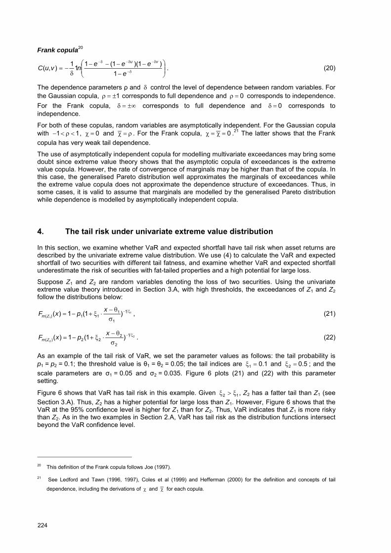
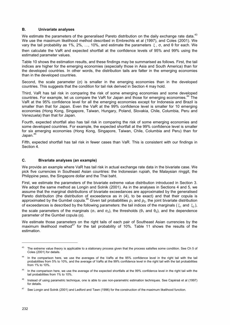
Example 2: Credit portfolio (Lucas et al (2001))

The next example demonstrates the tail risk of VaR in a credit portfolio, using the result of Lucas et al (2001).

Lucas et al (2001) derive an analytic approximation to the credit loss distribution of large portfolios. To illustrate their general result, they provide a simple example of credit loss calculation.10 They consider a bond portfolio where the amount of credit exposure for individual bonds is identical and the default is triggered by a single factor. For simplicity, they assume that the loss is recognised in the default mode and that the factor sensitivities of the latent variables and default probabilities are homogeneous.11 They show that the credit loss of the bond portfolio converges almost surely to C, as defined in the following equation, when the number of bonds approaches infinity (Lucas et al (2001, p 1643, equation (14)).

��

�

�

��

�

�

��

��

21

YsC (1)

� :The distribution function of the standard normal distribution

Y :Random variable following the standard normal distribution

s :The value of )(1 p�

� when the default rate is p , and 1�� is the inverse of � .

� :Correlation coefficient among the latent variables

Based on this result, we calculate the distribution functions of the limiting credit loss C for ρ = 0.7 and 0.9, and plot them in Figure 2.

The results show that VaR has tail risk. The bond portfolio is more concentrated when ρ = 0.9 than when ρ = 0.7. The tail of the credit loss distribution is fatter when ρ = 0.9 than when ρ = 0.7. Thus, the

10 Lucas et al (2001) also develop more general analyses in their paper. 11 The total exposure of the bond portfolio is 1.

219

bond portfolio is more risky when ρ = 0.9 than when ρ = 0.7. However, the VaR at the 95% confidence interval is higher when ρ = 0.7 than when ρ = 0.9. This shows that VaR fails to consider credit concentration since it disregards the loss beyond the confidence level.

The preceding examples show that VaR has tail risk when the loss distributions intersect beyond the confidence level. In such cases, one is able to decrease VaR by manipulating the tails of the loss distributions. This manipulation of the distribution tails increases the potential for extreme losses, and may lead to a failure of risk management. This problem is significant when the portfolio profit/loss is non-linear and the distribution function of the profit/loss is discontinuous.12

B. The tail risk of expected shortfall We define the tail risk of expected shortfall in the same way as the tail risk of VaR. In this paper, we say that expected shortfall has tail risk when expected shortfall fails to summarise the relative choice between portfolios as a result of its underestimation of the risk of portfolios with fat-tailed properties and a high potential for large losses.

To illustrate our definition of the tail risk of expected shortfall, we present an example from Yamai and Yoshiba (2002c). Table 1 shows the payoff and profit/loss of two sample portfolios A and B. The expected payoff and the initial investment amount of both portfolios are equal at 97.05.

In most of the cases, both portfolios A and B do not incur large losses. The probability that the loss is less than 10 is about 99% for both portfolios.

The magnitude of extreme loss is different. Portfolio A never loses more than half of its value while Portfolio B may lose three quarters of its value. Thus, portfolio B is more risky than Portfolio A when one is worried about extreme loss.

Table 2 shows the VaR and expected shortfall of the two portfolios at the 99% confidence level. Both VaR and expected shortfall are higher for Portfolio A, which has a lower magnitude of extreme loss. Thus, expected shortfall has tail risk since it chooses the more risky portfolio as a result of its disregard of extreme losses.

The example above shows that expected shortfall may have tail risk. However, the tail risk of expected shortfall is less significant than that of VaR. Yamai and Yoshiba (2002c) show that expected shortfall has no tail risk under more lenient conditions than VaR. This is because VaR completely disregards any loss beyond the confidence level while expected shortfall takes this into account as a conditional expectation.

3. Multivariate extreme value theory

In this section, we give a brief introduction to multivariate extreme value theory.13 We use this theory to represent asset returns under market stress in the following sections.

Multivariate extreme value theory consists of two modelling aspects: the tails of the marginal distributions and the dependence structure among extreme values.

We restrict our attention to the bivariate case in this paper.

12 Yamai and Yoshiba (2002c) show that VaR has no tail risk when the loss distributions are of the same type of an elliptical

distribution. 13 For detailed explanations of extreme value theory, see Coles (2001), Embrechts et al (1997), Kotz and Nadarajah (2000)

and Resnick (1987).

220

A. Univariate extreme value theory Let Z denote a random variable and F the distribution function of Z. We consider extreme values in terms of exceedances with a threshold � ( 0�� ). The exceedances are defined as ),max()( ��

�ZZm .

Z is larger than θ with probability p, and smaller than θ with probability 1 � p. Then, by the definition of exceedances, )(1 �� Fp . We call p tail probability.

The conditional distribution Fθ defined below gives the stochastic behaviour of extreme values.

)(1)()(}Pr{)(

��

��

� FFxFZxZxF , x�� . (2)

This is the distribution function of (Z � θ) given that Z exceeds θ. Fθ is not known precisely unless F is known.

The extreme value theory tells us the approximation to Fθ that is applicable for high values of threshold θ. The Pickands-Balkema-de Haan theorem shows that as the value of θ tends to the right end point of F, Fθ converges to a generalised Pareto distribution. The generalised Pareto distribution is represented as follows:14, 15

��

��

��1

, )1(1)( xxG , 0�x . (3)

With equations (1) and (2), when the value of θ is sufficiently large, the distribution function of exceedances mθ(Z), denoted by Fm(x), is approximated as follows:

��

��

��

1, )1(1)()())(1()( xpFxGFxFm , ��x . (4)

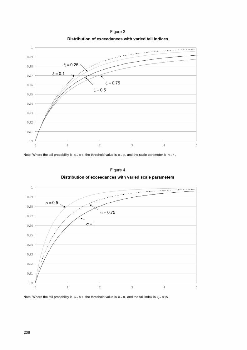
In this paper, we call Fm(x) the distribution of exceedances.

The distribution of exceedances is described by three parameters: the tail index � , the scale parameter σ, and the tail probability p. The tail index � represents how fat the tail of the distribution is, so the tail is fat when � is large (see Figure 3). The scale parameter σ represents how dispersed the distribution is, so the distribution is dispersed when σ is large (see Figure 4). The tail probability p determines the threshold θ as pFm �� 1)( .

When the confidence level of VaR and expected shortfall is less than p, the distribution of exceedances is used to calculate VaR and expected shortfall. (See Section 4 for the specific calculations.)

B. Copula As a preliminary to the dependence modelling of extreme values, we provide a simple explanation of copula.16

Suppose we have two-dimensional random variables (Z1,Z2). Their joint distribution function ],[),( 221121 xZxZPxxF �� fully describes their marginal behaviour and dependence structure. The

main idea of copula is that we separate this joint distribution into the part that describes the dependence structure and the part that describes the marginal behaviour.

Let (F1(x1),F2(x2)) denote the marginal distribution functions of (Z1,Z2). Suppose we transform (Z1,Z2) to have standard uniform marginal distributions.17 This is done by ))(),((),( 221121 ZFZFZZ � . The joint

14 See Coles (2001) and Embrechts et al (1997) for a detailed explanation of this theorem. 15 In this paper we assume that 0�� . 16 For the precise definition of copula and proofs of the theorems adopted here, see eg Embrechts et al (2002), Joe (1997),

Nelsen (1999) and Frees and Valdez (1998). 17 The standard uniform distribution is the uniform distribution over the interval [0,1].

221

distribution function C of the random variable (F1(Z1),F2(Z2)) is called the copula of the random vector (Z1,Z2). It follows that:

))(),((],[),( 2211221121 xFxFCxZxZPxxF �� . (5)

Sklar�s theorem shows that (4) holds with any F for some copula C and that C is unique when F1(x1) and F2(x2) are continuous.

In general, the copula is defined as the distribution function of a random vector with standard uniform marginal distributions. In other words, the distribution function C is a copula function for the two random variables 21,UU that follow the standard uniform distribution.

],Pr[),( 221121 uUuUuuC �� . (6)

One of the most important properties of the copula is its invariance property. This property says that a copula is invariant under increasing and continuous transformations of the marginals. That is, when the copula of (Z1,Z2) is C(u1,u2) and )(),( 21 hh are increasing continuous functions, the copula of (h1(Z1),h2(Z2)) is also C(u1,u2).

The invariance property and Sklar�s theorem show that a copula is interpreted as the dependence structure of random variables. The copula represents the part that is not described by the marginals, and is invariant under the transformation of the marginals.

C. Multivariate extreme value theory We give a brief illustration of the bivariate exceedances approach as a model for the dependence structure of extreme values.18

Let ),( 21 ZZZ � denote the two-dimensional vector of random variables and ),( 21 ZZF the distribution function of Z . The bivariate exceedances of Z correspond to the vector of univariate exceedances defined with a two-dimensional vector of threshold ),( 21 �� (see Figure 5). These exceedances are defined as follows:

)),max(),,(max(),( 221121),( 21��

��ZZZZm . (7)

The marginal distributions of the bivariate exceedances defined in (6) converge to the distribution of exceedances introduced in Section 3.A when the thresholds tend to the right end points of the marginal distributions. This is because the bivariate exceedance is the vector of univariate exceedances whose distribution converges to a generalised Pareto distribution.

The copula of bivariate exceedances also converges to a class of copula that satisfies several conditions. Ledford and Tawn (1996) show that this class is represented by the following equation (see Appendix A for details):

)}log

1,log

1(exp{),(21

21 uuVuuC �� , (8)

where

��

��

1

01

21

121 )(})1(,max{),( sdHzsszzzV , (9)

and H is a non-negative measure on [0,1] satisfying the following condition:

1)()1()(1

0

1

0�� sdHsssdH . (10)

Following Hefferman (2000), we call this type of copula the bivariate extreme value copula or the extreme value copula.

18 For more detailed explanations of multivariate extreme value theory, see Coles (2001) Ch 8 , Kotz and Nadarajah (2000)

Ch 3, McNeil (2000), Resnick (1987) Ch 5, etc.

222

The class of the extreme value copula is wide, being constrained only by (9). We have an infinite number of parameterised extreme value copulas. In practice, we choose a parametric family of copula that satisfies (9), and use the copula for the analysis of bivariate extreme values.

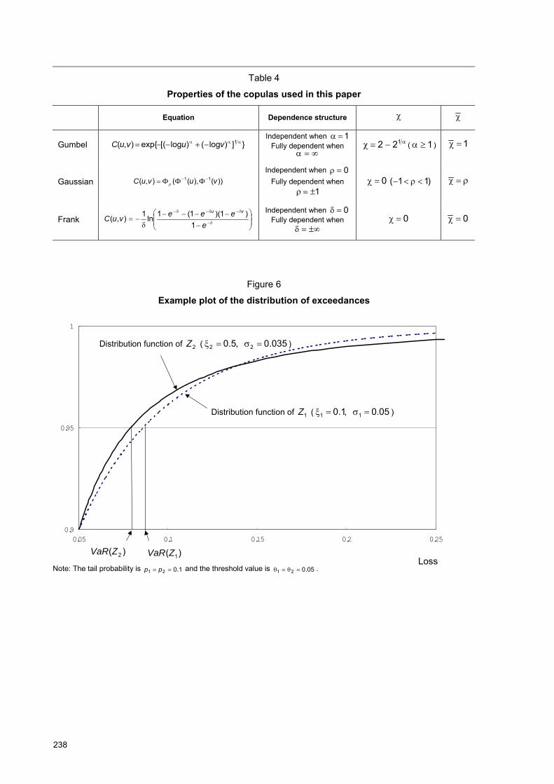
One standard type of bivariate extreme value copula is the Gumbel copula. The Gumbel copula is the most frequently used extreme value copula for applied statistics, engineering and finance (Gumbel (1960), Tawn (1988), Embrechts et al (2002), McNeil (2000), Longin and Solnik (2001)). The Gumbel copula is expressed by:

}])log()log[(exp{),( 12121

��

�� uuuuC , (11)

for a parameter ],1[ �� . We obtain (10) by defining V in (8) as follows:

��

��1

2121 )(),( zzzzV . (12)

The dependence parameter α controls the level of dependence between random variables. α = 1 corresponds to full dependence and �� corresponds to independence.

The Gumbel copula has several advantages over other parameterised extreme value copulas.19 It includes the special cases of independence and full dependence, and only one parameter is needed to model the dependence structure. The Gumbel copula is tractable, which facilitates simulations and maximum likelihood estimations. Given these advantages, we adopt the Gumbel copula as the extreme value copula.

To summarise, extreme value theory shows that the bivariate exceedances asymptotically follow a joint distribution whose marginals are the distributions of exceedances and whose copula is the extreme value copula.

D. Tail dependence We introduce the concept of tail dependence between random variables. Suppose that a random vector (Z1,Z2) has a joint distribution function F(Z1,Z2) with marginals F1(x1),F2(x2).

Assume that marginals are equal. We define a dependence measure � as follows:

}Pr{lim 21 zZzZzz

��

�

, (13)

where �z is the right end point of F.

� measures the asymptotic survival probability over one value to be large given that the other is also large. When 0�� , we say Z1 and Z2 are asymptotically independent. When 0�� , we say Z1 and Z2 are asymptotically dependent. � increases with the strength of dependence within the class of asymptotically dependent variables.

When F has different marginals 1ZF and

2ZF , � is defined as follows:

})()(Pr{lim 211 21uZFuZF ZZu

��

. (14)

Further defining the other dependence measure )(u� as in (14), the relationship )(lim1

uu

��

holds

(Coles et al (1999)).

})(Pr{log})(,)(Pr{log

2)(1

21

1

21

uZFuZFuZF

uZ

ZZ

�

�� , for 10 �� u . (15)

19 For other parameterised extreme value copulas, see, for example, Joe (1997) and Kotz and Nadarajah (2000).

223

Although � measures dependence when random variables are asymptotically dependent, it fails to do so when random variables are asymptotically independent. When random variables are asymptotically independent, 0�� by definition and � is unable to provide dependence information.

The class of asymptotically independent copulas includes important copulas such as the Gaussian copula and the Frank copula, which are introduced in the next section. Ledford and Tawn (1996, 1997) and Coles et al (1999) say that the asymptotically independent case is important in the analysis of multivariate extreme values.

To counter this shortcoming of the dependence measure � , Coles et al (1999) propose a new dependence measure � as defined below.

)(lim1

uu

��

(16)

where 1})(,)(Pr{log

})(Pr{log2)(

21

1

21

1 ��

��

uZFuZFuZF

uZZ

Z (17)

� measures dependence within the class of asymptotically independent variables. For asymptotically independent random variables, 11 �� . For asymptotically dependent random variables, 1�� .

Thus, the combination ),( �� measures tail dependence for both asymptotically dependent and independent case (see Table 3). For asymptotically dependent random variables, 1�� and � measures tail dependence. For asymptotically independent random variables, 0�� and � measures tail dependence.

E. Copula and tail dependence

With some calculations, it is shown that )(u� is constant for the bivariate extreme value copula as follows:

)1,1(2)( Vu �� . for all 10 �� u . (18)

For the Gumbel copula, this becomes �

��122 ( 1�� ) (see Table 4). Thus, for the bivariate extreme

value copula, random variables are either independent or asymptotically dependent. In other words, the bivariate extreme copula is unable to represent the dependence structure when random variables are asymptotically independent.

Ledford and Tawn (1996, 1997) and Coles (2001) say that multivariate exceedances may be asymptotically independent and that modelling multivariate exceedances with the extreme value copula is likely to lead to misleading results in this case. They say that the use of asymptotically independent copulas is effective when the multivariate exceedances are asymptotically independent. Hefferman (2000) provides a list of asymptotically independent copulas that are useful for modelling multivariate extreme values.

In this paper, we adopt the Gaussian copula and the Frank copula as asymptotically independent copulas. These are defined as follows (see Table 4).

Gaussian copula

))(),((),( 11 vuvuC ��

�� (19)

where �

� is the distribution function of a bivariate standard normal distribution with a correlation

coefficient ρ, and 1�� is the inverse function of the distribution function for the univariate standard

normal distribution.

224

Frank copula20

��

��

�

�

��

��

��

��

eeeenvuC

vu

1)1)(1(111),( . (20)

The dependence parameters ρ and � control the level of dependence between random variables. For the Gaussian copula, 1�� corresponds to full dependence and 0�� corresponds to independence. For the Frank copula, �� corresponds to full dependence and 0�� corresponds to independence.

For both of these copulas, random variables are asymptotically independent. For the Gaussian copula with 11 �� , 0�� and �� . For the Frank copula, 0�� .21 The latter shows that the Frank copula has very weak tail dependence.

The use of asymptotically independent copula for modelling multivariate exceedances may bring some doubt since extreme value theory shows that the asymptotic copula of exceedances is the extreme value copula. However, the rate of convergence of marginals may be higher than that of the copula. In this case, the generalised Pareto distribution well approximates the marginals of exceedances while the extreme value copula does not approximate the dependence structure of exceedances. Thus, in some cases, it is valid to assume that marginals are modelled by the generalised Pareto distribution while dependence is modelled by asymptotically independent copula.

4. The tail risk under univariate extreme value distribution

In this section, we examine whether VaR and expected shortfall have tail risk when asset returns are described by the univariate extreme value distribution. We use (4) to calculate the VaR and expected shortfall of two securities with different tail fatness, and examine whether VaR and expected shortfall underestimate the risk of securities with fat-tailed properties and a high potential for large loss.

Suppose Z1 and Z2 are random variables denoting the loss of two securities. Using the univariate extreme value theory introduced in Section 3.A, with high thresholds, the exceedances of Z1 and Z2 follow the distributions below:

1

1

1

1

111)( )1(1)( ��

�

��xpxF Zm , (21)

2

2

1

2

222)( )1(1)( ��

�

��xpxF Zm . (22)

As an example of the tail risk of VaR, we set the parameter values as follows: the tail probability is p1 = p2 = 0.1; the threshold value is θ1 = θ2 = 0.05; the tail indices are 1.01 �� and 5.02 �� ; and the scale parameters are σ1 = 0.05 and σ2 = 0.035. Figure 6 plots (21) and (22) with this parameter setting.

Figure 6 shows that VaR has tail risk in this example. Given 12 �� , Z2 has a fatter tail than Z1 (see Section 3.A). Thus, Z2 has a higher potential for large loss than Z1. However, Figure 6 shows that the VaR at the 95% confidence level is higher for Z1 than for Z2. Thus, VaR indicates that Z1 is more risky than Z2. As in the two examples in Section 2.A, VaR has tail risk as the distribution functions intersect beyond the VaR confidence level.

20 This definition of the Frank copula follows Joe (1997).

21 See Ledford and Tawn (1996, 1997), Coles et al (1999) and Hefferman (2000) for the definition and concepts of tail

dependence, including the derivations of � and � for each copula.

225

We derive the conditions for the tail risk of VaR. Following McNeil (2000), we calculate the VaR from (21) and (22). Let VaRα(Z) denote the VaR of Z at the (1 � α) confidence level. Since VaR is the upper (1 � α) quantile of the loss distribution, the following holds:

��

�

��

1))(1(11 ZVaRp . (23)

We then solve (23) to obtain the following:

��

�

�

��

�

��

�

��

��

��

�

� 1)( pZVaR . (24)

With (24), we derive the condition of the tail risk of VaR as follows. Without the loss of generality, we assume 12 �� , or that the tail of Z2 is fatter than the tail of Z1. In other words, Z2 has higher potential for extreme loss than Z1. VaR has tail risk when the VaR of Z2 is smaller than that of Z1, or when the following inequality holds:

)()( 21 ZVaRZVaR��

. (25)

Assuming θ1 = θ2 and p1 = p2 = p for simplification, we obtain the following condition from (24) and (25):

VaR��

�

�

2

1 , where � ��

��

��

�

��

��

�

�

�

11

1

2

2

1

pp

VaR . (26)

The value VaR� indicates how strict the condition for the tail risk of VaR is. When VaR� is small, a small difference between the scale parameters σ1 and σ2 brings about tail risk of VaR. When VaR� is large, a large difference between σ1 and σ2 is needed to bring about tail risk of VaR.

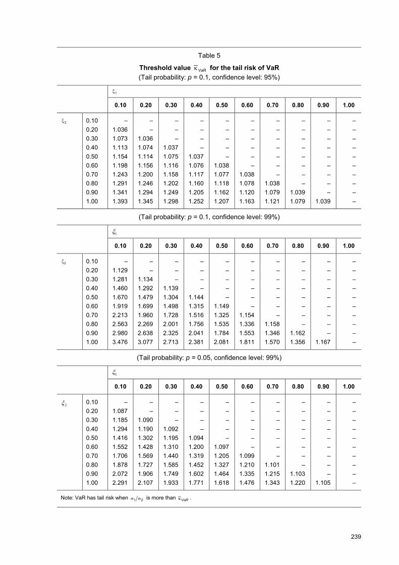
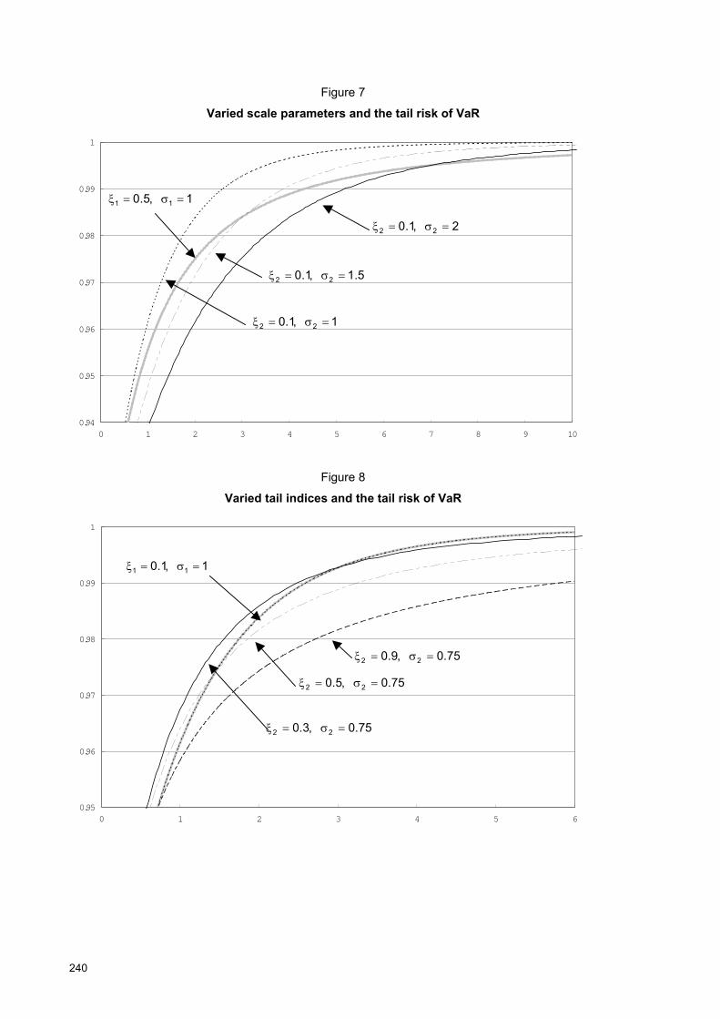
Table 5 shows the value of VaR� with varying ),( 21 �� for VaR at the 95% and 99% confidence levels, when p is 0.05 and 0.1.22 This table shows two aspects of this condition.

First, the scale parameter of the thin-tailed distribution σ1 must be larger than the scale parameter of the fat-tailed distribution σ2. This is because 1��VaR for all combinations of ),( 21 �� .

Figure 7 illustrates this point. The figure plots the distribution of exceedance with parameter values 1,5.0 11 �� . The figure also plots the distribution of exceedances with parameter values 1.02 ��

and 12 �� , 1.5 and 2. Here, we denote the VaR for 1,5.0 11 �� as )1,5.0( 11 ��VaR and that for �� 22 ,1.0 as ),1.0( 22 ��VaR . The distribution with 5.01 �� has a fatter tail and higher potential for large loss than the distribution with 1.02 �� . Thus, VaR has tail risk if

),1.0()1,5.0( 2211 �� VaRVaR .

From the figure, we find )2,1.0()1,5.0( 2211 �� VaRVaR with a confidence level below 99%, and )5.1,1.0()1,5.0( 2211 �� VaRVaR with a confidence level below 98%. On the other hand, )1,1.0()1,5.0( 2211 �� VaRVaR with a confidence level above 95%. Therefore, VaR has tail risk with a high confidence level when the difference between the scale parameters is large.

Second, the smaller the difference between the tail indices 1� and 2� , the more lenient the conditions for the tail risk of VaR. This is because VaR� is small when the difference between the tail indices is small.

Figure 8 illustrates this point. The figure plots the distribution of exceedances with parameter values 1,1.0 11 �� . The figure also plots the distribution of exceedances with parameter values 75.02��

22 When the tail probability is p = 0.05, the VaR at the confidence level of 95% is not beyond the threshold, so we do not

calculate VaR at the confidence level of 95% when p = 0.05.

226

and 9.0,5.0,3.02 �� . Here, we denote the VaR for 1,1.0 11 �� as )1,1.0( 11 ��VaR and that for 75.0, 22 �� as )75.0,( 22 ��VaR . As the distribution tail is fatter with 75.0, 22 �� than with 1,1.0 11 �� , VaR has tail risk if )75.0,()1,1.0( 2211 �� VaRVaR . We find

)1,1.0( 11 ��VaR )75.0,3.0( 22 �� VaR with a confidence level below 99%, and )75.0,5.0()1,1.0( 2211 �� VaRVaR with a confidence level below 97%. On the other hand, )75.0,9.0()1,1.0( 2211 �� VaRVaR with a confidence level above 95%. Therefore, VaR has

tail risk with a high confidence level when the difference between the tail indices is small.

We analyse the condition for the tail risk of expected shortfall as we analysed that of VaR. Following McNeil (2000), we can calculate the expected shortfall of Z at the (1 � α) confidence level (denoted by ESα(Z)) from (24).23

.11111

)(1

1))((

)(

])(|))(()[)()](|[)(

��

��

��

��

��

��

�

��

��

��

��

��

��

��

��

��

��

��

��

�

�

�

�

��

��

pZVaR

ZVaRZVaR

ZVaRZZVaRZEZVaRZVaRZZEZES

(27)

Given 12 �� , expected shortfall has tail risk when the following inequality holds:

)()( 21 ZESZES��

� . (28)

Assuming θ1 = θ2 and p1 = p2 = p for simplification, we obtain the following condition from (27) and (28):

ES� �

�

2

1 , where � ��

��

��

�

��

��

��

��

�

�

1

2

2

1

1111

11

1

2

pp

ES . (29)

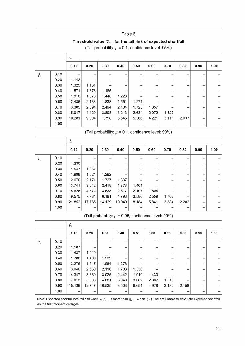
Table 6 shows the value of ES� with varying ),( 21 �� for expected shortfall at the 95% and 99% confidence levels, when p is 0.05 and 0.1.24 This table shows that the conditions for the tail risk of expected shortfall are stricter than those for the tail risk of VaR. This confirms the result of Yamai and Yoshiba (2002c) that expected shortfall has no tail risk under more lenient conditions than VaR.

To summarise, VaR and expected shortfall may underestimate the risk of securities with fat-tailed properties and a high potential for large loss. The condition for tail risk to emerge depends on the parameters of the loss distribution and the confidence level.

5. The tail risk under multivariate extreme value distribution

The use of risk measures may lead to a failure of risk management when they fail to consider the change in dependence between asset returns. The credit portfolio example in Section 2.A shows that VaR disregards the increase in default correlation and thus fails to note the high potential for extreme loss in concentrated credit portfolios. In this case, the use of VaR for credit portfolios may lead to credit concentration.

In this section, we examine whether VaR and expected shortfall disregard the changes in dependence under a multivariate extreme value distribution. As the multivariate extreme value distribution, we use the joint distribution of exceedances introduced in Section 3.C. The marginal of this distribution is the

23 The third equality is based on Embrechts et al (1997), Theorem 3.4.13 (e). 24 We do not calculate expected shortfall at the confidence level of 95% when p = 0.05 (see footnote 22).

227

generalised Pareto and its copula is the Gumbel copula. We also use the Gaussian and Frank copulas for the copulas of exceedances for the case where the exceedances are asymptotically independent.

A. The difficulty of applying multivariate extreme value distribution to risk measurement The application of multivariate extreme value distribution to financial risk measurement has some problems that the univariate application does not. In the univariate case, the model for exceedances enables us to calculate VaR and expected shortfall as in Section 4. This is because the VaR and expected shortfall of exceedances are equal to the VaR and expected shortfall of the original loss data. However, in the multivariate case, the model for exceedances is not sufficient to calculate VaR and expected shortfall. This is because, in the multivariate case, the sum of exceedances is not necessarily equal to the exceedances of the sum. To calculate VaR and expected shortfall, we need the exceedances of the sum, which are unavailable from the model for exceedances alone.25, 26, 27

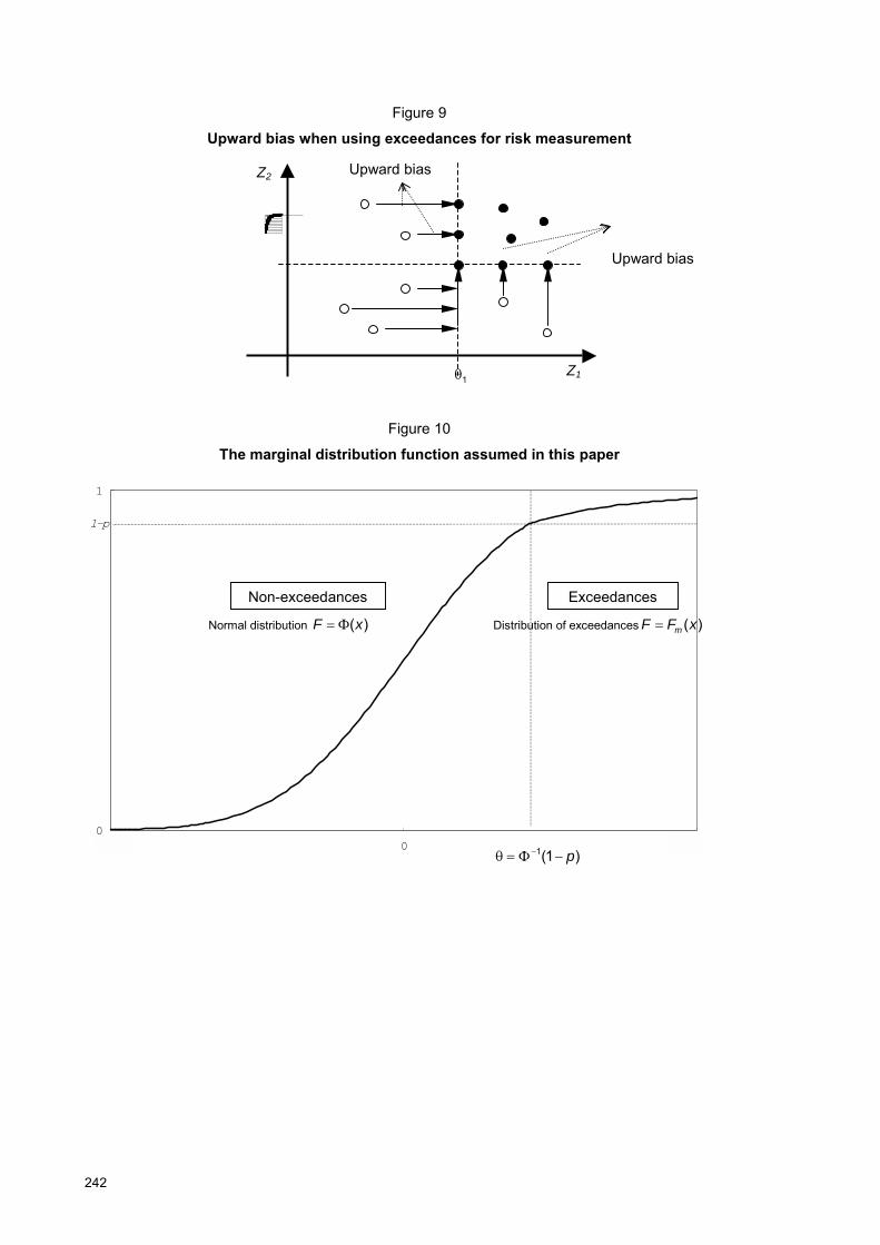
A simple example illustrates this point (Figure 9). Let (U1,U2) denote a vector of independent standard uniform random variables. With a threshold value of )9.0,9.0(),( 21 �� , the exceedances of (U1,U2) are

))(),(( 29.019.0 UmUm ))9.0,max(),9.0,(max( 21 UU� . With the convolution theorem, the 95% upper quantile of U1 + U2 is calculated to be 1.68, while that of )()( 21 21

UmUm��

� is calculated to be 1.88.28 Thus, the sum of exceedances is larger than the exceedances of the sum.

This example shows that, to calculate VaR and expected shortfall in the multivariate case, we need a model for non-exceedances as well as one for exceedances.

In this paper, we assume that the marginal distribution of the non-exceedances is the standard normal distribution as we interpret the non-exceedances as asset loss under normal market conditions. That is, we assume that the marginal distribution is expressed by (30) below (Figure 10): 29

25 This is also a problem when the model for maxima is used for calculating VaR and expected shortfall. This is because the

sums of maxima are not necessarily equal to the maxima of sums. Hauksson et al (2000) and Bouyé (2001) propose the use of multivariate generalised extreme value distributions for financial risk measurement, but they do not address this problem.

26 The quantile of the sum of exceedances is equal to that of the original data when the underlying random variables are fully dependent.

27 McNeil (2000) says that multivariate extreme value modelling has the problem of �the curse of dimensionality�. He notes that, when the number of dimension is more than two, the estimation of copula is not tractable.

28 The upper 95% quantile of U1 + U2 is calculated as follows. Denote the distribution function of U1 + U2 as G(x). Clearly, the upper 95% quantile of U1 + U2 is greater than 1. So assuming x > 1, G(x) is calculated by the convolution theorem as follows:

1)2(21]Pr[)( 21

0 1 �� xduuxUxG

The upper 95% quantile is x that satisfies G(x) = 0.95, which is calculated as 6838.1�x .

The upper 95% quantile of the sum of the exceedances is calculated as follows. Define �)(xH ])9.0,max()9.0,Pr[max( 21 xUU �� . Using the convolution theorem, this is restated as follows:

��

��

��

�� )9.1(12)2(

)9.1(81.02])9.0,Pr[max(])9.0,Pr[max()( 2

21

0 21 xxxxduuUuxUxH

The upper 95% quantile is x that satisfies G(x) = 0.95, which is calculated as 8761.1�x . 29 A different assumption might be that the marginal distribution of exceedances is a non-standard normal distribution, a

t-distribution, a generalised Pareto distribution, or an empirical distribution produced from actual data. Assuming a non-standard normal distribution, a t-distribution, and a generalised Pareto distribution, we simulated asset loss as in sections B and C of this chapter, and found the same result as in those sections. Furthermore, under the assumption of a generalised Pareto distribution, the convolution theorem is applied to obtain the analytics of the tail risk of VaR (see Appendix B for the details).

228

��

��

�

��

��

��

��

�

)).1(())1(1(1

)),1(()()( 11

1

1

pxpxp

pxxxF (30)

� :the distribution function of the standard normal 1�� :the inverse function of �

In the following analysis, we simulate two dependent asset losses to analyse the tail risk of VaR and expected shortfall.30 In the simulation, we assume that the marginal distribution of asset loss is (30). We also assume that the copula of asset loss is one of three copulas introduced in Section 3.E: Gumbel, Gaussian and Frank. We set the marginal distribution of each asset loss as identical so that we can examine the pure effect of dependence on the tail risk of VaR and expected shortfall. We limit our attention to the cases where the tail index is 10 �� .31

B. One specific copula case In this section, we assume that the change in the dependence structure of asset loss is represented by the change in the dependence parameters within one specific copula. Under this assumption, we examine whether VaR and expected shortfall consider the change in dependence by taking the following steps. First, we take one of the three copulas introduced in Section 3.E: Gumbel, Gaussian or Frank. Second, we simulate asset losses under the one copula for varied dependence parameter levels (Gumbel: α, Gaussian: ρ, and Frank: � ). Third, we calculate VaR and expected shortfall with the simulated asset losses for each dependence parameter level.

If VaR and expected shortfall do not increase with the rise in the level of dependence, VaR and expected shortfall disregard dependence and thus have tail risk.

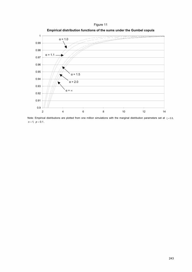
Figure 11 shows an example of this analysis. The figure plots the empirical distribution of the sum of two simulated asset losses. These losses are simulated adopting (30) as the marginals and the Gumbel copula as the copula. The parameters of the marginal are set at 1.0,1,5.0 �� p , and the dependence parameter α of the Gumbel copula is set at 1.0, 1.1, 1.5, 2.0 and � .32 For each dependence parameter, we conduct one million simulations.

The result shows that the distribution tail gets fatter as the value of the dependence parameter α increases, or the asset losses are more dependent. Furthermore, the empirical distributions do not intersect with each other. This shows that the portfolio diversification effect works to decrease the risk of the portfolio and that VaR has no tail risk regardless of its confidence level.

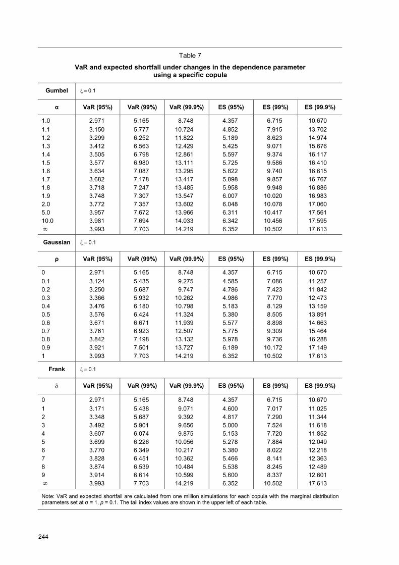
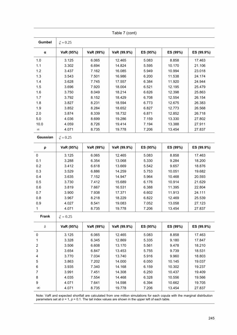
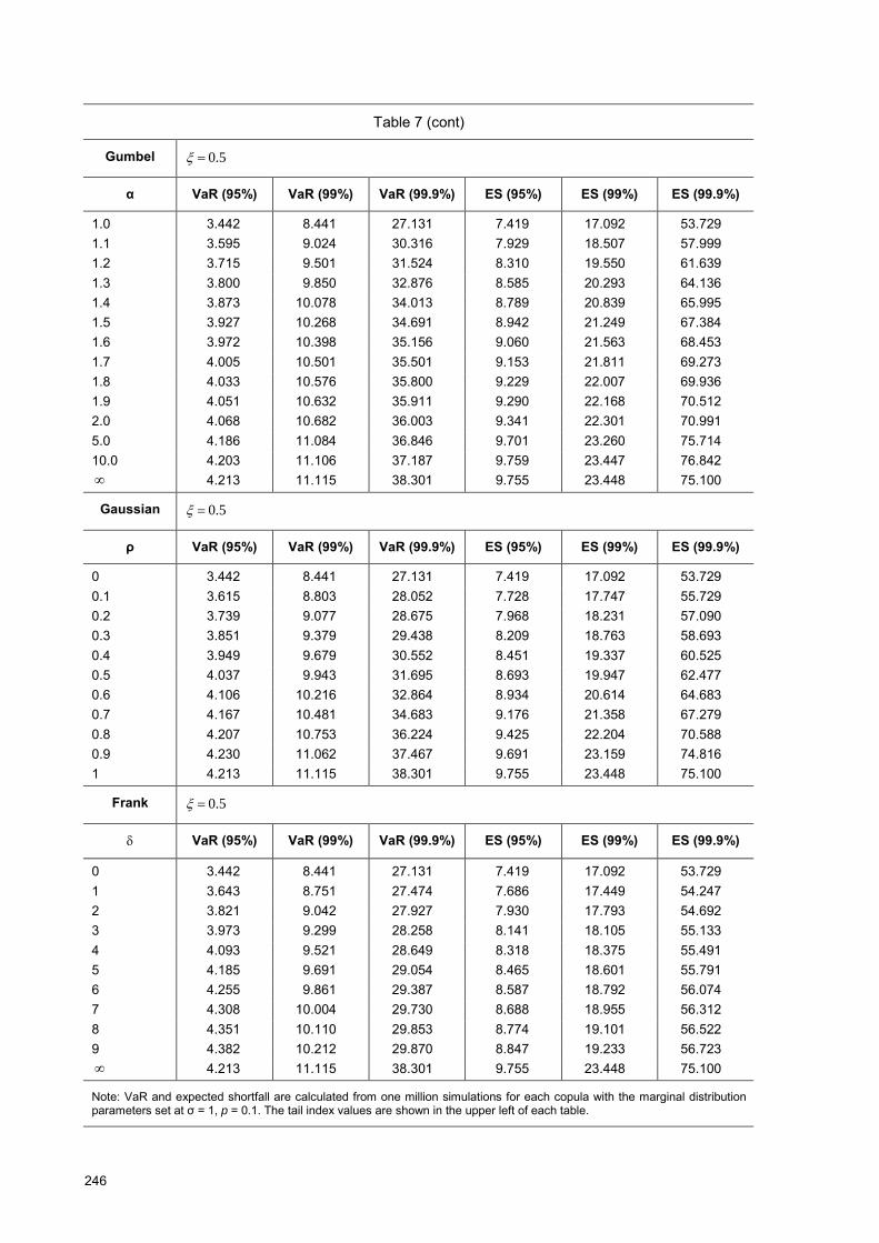
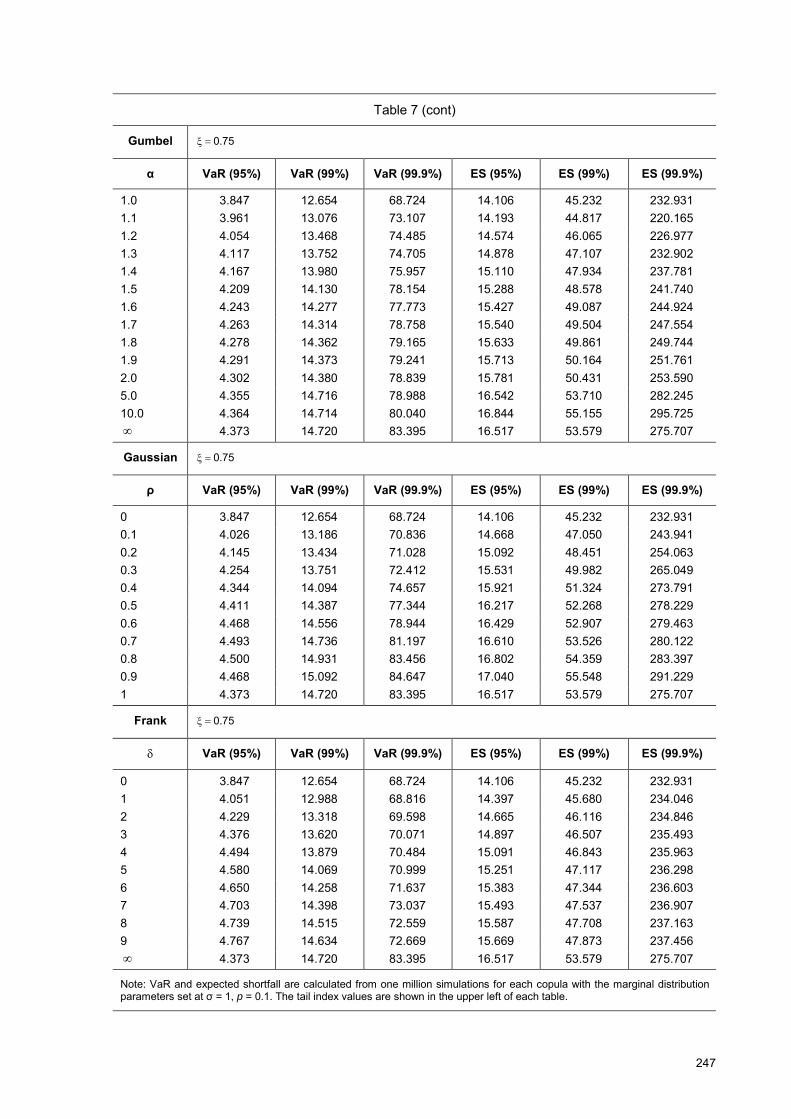
Table 7 provides a more general analysis. The figure gives the VaR and expected shortfall under one million simulations for each copula with various dependence parameter levels. Two of the three marginal distribution parameters ),,( p�� are set at σ = 1, p = 0.1, and the tail index � is set at 0.1, 0.25, 0.5 and 0.75. One of the copulas (Gumbel, Gaussian and Frank) is adopted. With these marginals and copulas, asset losses are simulated. VaR and expected shortfall are calculated for varied dependence parameter levels (Gumbel: α, Gaussian: ρ, and Frank: � ).

30 We use the Mersenne Twister for generating uniform random numbers, and the Box-Müller method for transforming the

uniform random numbers into normal random numbers. We follow Frees and Valdez (1998) in simulating the Gumbel copula, and Joe (1997) for simulating the Gaussian and Frank copulas.

31 The generalised Pareto distribution with 1�� is so fat-tailed that its mean is infinite (Embrechts et al (1997), Theorem 3.4.13 (a)).

The generalised Pareto distribution with 1�� has several interesting properties. However, it is not considered in this paper because such a fat-tailed distribution is rarely observed in financial data. For details, see Appendix B.

32 Under the Gumbel copula ��

122 , so the corresponding values of � become 1,59.0,41.0,12.0,0�� .

229

Table 7 shows that VaR and expected shortfall consider the change in dependence and have no tail risk in most of the cases. VaR and expected shortfall increase as the value of the dependence parameter rises, except for the Frank copula with extremely high dependence parameter levels.33

To summarise, VaR and expected shortfall have no tail risk when the change in dependence is represented by the change in parameters using one specific copula. Thus, if we select portfolios whose dependence structure is nested in one of the three copulas above, we can depend on VaR and expected shortfall for measuring dependent risks.

C. Different copulas case In the previous section, we assume that the change in the dependence of asset losses is represented by the change in the parameters using one specific copula. However, this assumption has a problem. One specific copula does not represent both asymptotic dependence and asymptotic independence.

Let us consider an example of this problem. Suppose we have two portfolios both composed of two securities. Also suppose that the security returns of one portfolio are asymptotically dependent while those of the other are asymptotically independent. Adopting one specific copula and changing the dependence parameters to describe the change in dependence does not work in this case. This is because one specific copula does not represent the change from asymptotic dependence to asymptotic independence. We need different types of copulas to compare asymptotic dependence with asymptotic independence.

In this section, we assume that the change in dependence is represented by the change in copula. We adopt the Gumbel, Gaussian and Frank copulas introduced in Section 3.E since the Gumbel copula corresponds to asymptotic dependence and the Gaussian and Frank copulas correspond to asymptotic independence. By changing copula from Gumbel to Gaussian and Frank, we can change the dependence structure from asymptotic dependence to asymptotic independence.

In comparing the results with three copulas, we set the values of the dependence parameters of those copulas (Gumbel: α, Gaussian: ρ, and Frank: � ) so that the Spearman�s rho (ρs) is equal across those copulas.34,35 By setting the Spearman�s rho equal, we can eliminate the effect of global dependence and examine the pure effect of tail dependence since the Spearman�s rho is a measure of global dependence.

The upper half of Figure 12 shows the empirical distributions of the sums of two simulated asset losses for the Gumbel, Gaussian and Frank copulas. This is generated from one million simulations for each copula where the parameters are fixed at 1.0,5.0,1,5.0 �� pS . The range of the horizontal axis (cumulative probability) is above 99.5%.

The tail shape of the loss distribution for each copula is consistent with the tail dependence of each copula. The empirical loss distribution for the Gumbel copula, which is asymptotically dependent

33 In the case of the Frank copula, the VaR at the 95% confidence level when �� (full dependence) is smaller than the VaR

when 9�� .

This might be because the Frank copula has low tail dependence ( 0�� ) and does not represent tail dependence when � is large.

34 The Spearman�s rho is the linear correlation of the marginals, and is defined by the following equation:

)]([)]([

))(),((),(

21

2121

21

21

ZFVZFV

ZFZFCovZZ

ZZ

ZZS ��

.

The Spearman�s rho differs from � and � in that it measures global dependence while � and � measure tail dependence.

The Spearman�s rho does not fully represent the dependence structures since the combination of the Spearman�s rho and the marginal distribution does not uniquely define the joint distribution. In particular, it does not represent the asymptotic dependence measured by � and � . Nevertheless, the Spearman�s rho is relatively superior as a single measure of global dependence (see Embrechts et al (2002)).

35 We use the calculation in Joe (1997, p 147, Table 5.2) for the values of the dependence parameters that equate the Spearman�s rho.

230

� �1,0 �� , has the fattest tail. The empirical loss distribution for the Frank copula, which has the weakest tail dependence � �0,0 �� , has the thinnest tail.36

This shows that the potential for extreme loss is high when the tail dependence is high. Thus, if we are worried about extreme loss, portfolios with higher tail dependence should be considered more risky than those with lower tail dependence. As for the three copulas adopted here, we should consider the Gumbel copula as the most risky and the Frank copula the least risky in terms of tail risk. In this context, VaR and expected shortfall have tail risk when they do not increase in the order of Frank, Gaussian and Gumbel copulas.

The lower half of Figure 12 shows that VaR has tail risk in this example. The figure shows that the VaR at the 95% confidence level increases in the order of Gumbel, Gaussian and Frank. VaR says that the Gumbel copula is the least risky while the Frank copula is the most risky. This contradicts our observation of the upper tail described above.

Table 8 provides a more general analysis. The table shows the results of VaR and expected shortfall calculations for one million simulations for each copula with the tail index of the marginal distribution of �� 0.1, 0.25, 0.5, and 0.75, and Spearman�s rho of ρS = 0.2, 0.5 and 0.8.

The findings of the analysis are threefold. First, VaR and expected shortfall vary depending on the copula adopted. This means that the type of copula affects the level of VaR and expected shortfall. The difference is large when the tail index and the Spearman�s rho are large.

Second, VaR at the 95% confidence level has tail risk when the tail index � is 0.25 or higher. For example, when 5.0�� and ρS = 0.8, the VaR at the 95% confidence level is largest for the Frank copula and smallest for the Gumbel copula. On the other hand, VaR at the 99% and 99.9% confidence level has no tail risk, except when the tail is as fat as 75.0�� .

Third, expected shortfall has no tail risk at the 95, 99, or 99.9% confidence level, except when the tail is as fat as 75.0�� . This confirms the result of Yamai and Yoshiba (2002c) that expected shortfall has no tail risk under more lenient conditions than VaR.

D. Different marginals case In Sections 5.B and 5.C, the marginal distributions are assumed to be identical. In financial data, however, the distributions of asset returns are rarely identical. In this section, we extend our analysis to the different marginals case. We examine whether the conclusions in Sections 5.B and 5.C are still valid when the marginal distributions are different.

1. Independence vs full dependence case

We examine whether the results in Section 5.B (the specific copula case) are still valid when the marginal distributions are different. We compare independence and full dependence, noting the fact that independence and full dependence are nested in the Gumbel, Gaussian and Frank copulas. When the VaR for independence is higher than the VaR for full dependence, VaR has tail risk.

We simulate independent and fully dependent asset losses with all combinations of parameters of the marginal distributions from ��1 0.1, 0.25, 0.5, 0.75, ��2 0.1, 0.25, 0.5, 0.75, σ1 = 1, σ2 = 1.00, 1.25, 1.5,�, 9.5, 9.75, 10. We set the number of simulations at one million for each parameter combination. We calculate VaR and expected shortfall for both independence and full dependence, and compare them to see whether they have tail risk. We adopt the tail probability of p = 0.1.

We found that the VaR for full dependence is never smaller than the VaR for independence.37 Thus, at least within this framework, VaR captures full dependence and independence when the marginal distributions are different.

36 See Figure 7 for the values of � and � for each copula.

231

2. Different copulas case

We next examine whether the results in Section 5.B (the different copulas case) are still valid when the marginal distributions are different. We follow the same steps as in Section 5.C except that we set different parameter levels for two marginal distributions.

Under each one of the three copulas, as in Section 5.B, we simulate asset losses following the same method used in the previous subsection.

We find that VaR at the 95% confidence level may have tail risk even when the distribution tail is not so fat as 25.0�� .38 This means that the conditions of the tail risk of VaR are more lenient when the marginals are different than when they are identical. Table 9 shows that, with a tail index of 1.0�� , VaR at the 95% confidence level has tail risk. VaR is larger for the Gaussian copula than for the Gumbel copula.39

On the other hand, at the confidence level of 99%, we find that VaR has tail risk only when the tail is as fat as 75.0�� .

6. Empirical analyses

In Sections 4 and 5, we examine the tail risk of VaR and expected shortfall under extreme value distributions. We summarise the results as follows.

In the univariate case, VaR and expected shortfall may underestimate the risk of securities with fat-tailed properties and a high potential for large losses. The conditions for this to happen are expressed by a simple analytical inequality.

In the multivariate case, VaR and expected shortfall may both disregard the tail dependence when the tails of the marginal distributions are fat.

In this section, we conduct empirical analyses with exchange rate data to confirm whether VaR and expected shortfall have tail risk in actual financial data. We focus on the following questions.

Do VaR and expected shortfall underestimate the risk of currencies with fat-tailed properties and a high potential for large losses in the univariate case?

Is there asymptotic dependence that may bring the tail risk of VaR and expected shortfall in the multivariate case?

A. Data The data used for the analyses are the daily logarithmic changes of exchange rates of three industrialised countries and 18 emerging economies.40,41,42 The raw historical data are the exchange rates per one US dollar from 1 November 1993 to 29 October 2001.

37 The results of this simulation are omitted here due to space restrictions. 38 See Footnote 37. 39 This finding was confirmed by running 10 million simulations. 40 The data are sourced from Bloomberg. 41 We set the exchange rate as constant over holidays at the levels of the previous business day. This treatment does not

affect our results as we estimate only the tails of distributions. 42 The currencies of developed countries are as follows: Japanese yen, the Deutsche mark and pound sterling. The currencies

of emerging economies are as follows: Hong Kong dollar, Indonesian rupiah, Malaysian ringgit, Philippine peso, Singapore dollar, South Korean won, new Taiwan dollar, Thai baht, Czech koruna, Hungarian forint, Polish zloty, Slovakian koruna, Brazilian real, Chilean peso, Colombian peso, Mexican new peso, Peruvian new sol and Venezuelan bolίvar.

232

B. Univariate analyses We estimate the parameters of the generalised Pareto distribution on the daily exchange rate data.43 We use the maximum likelihood method described in Embrechts et al (1997), and Coles (2001). We vary the tail probability as 1%, 2%, �, 10%, and estimate the parameters � , σ, and θ for each. We then calculate the VaR and expected shortfall at the confidence levels of 95% and 99% using the estimated parameter values.

Table 10 shows the estimation results, and these findings may be summarised as follows. First, the tail indices are higher for the emerging economies (especially those in Asia and South America) than for the developed countries. In other words, the distribution tails are fatter in the emerging economies than in the developed countries.

Second, the scale parameter (σ) is smaller in the emerging economies than in the developed countries. This suggests that the condition for tail risk derived in Section 4 may hold.

Third, VaR has tail risk in comparing the risk of some emerging economies and some developed countries. For example, let us compare the VaR for Japan and those for emerging economies.44 The VaR at the 95% confidence level for all the emerging economies except for Indonesia and Brazil is smaller than that for Japan. Even the VaR at the 99% confidence level is smaller for 10 emerging economies (Hong Kong, Singapore, Taiwan, Hungary, Poland, Slovakia, Chile, Columbia, Peru and Venezuela) than that for Japan.

Fourth, expected shortfall also has tail risk in comparing the risk of some emerging economies and some developed countries. For example, the expected shortfall at the 99% confidence level is smaller for six emerging economies (Hong Kong, Singapore, Taiwan, Chile, Columbia and Peru) than for Japan.45

Fifth, expected shortfall has tail risk in fewer cases than VaR. This is consistent with our findings in Section 4.

C. Bivariate analyses (an example) We provide an example where VaR has tail risk in actual exchange rate data in the bivariate case. We pick five currencies in Southeast Asian countries: the Indonesian rupiah, the Malaysian ringgit, the Philippine peso, the Singapore dollar and the Thai baht.

First, we estimate the parameters of the bivariate extreme value distribution introduced in Section 3. We adopt the same method as Longin and Solnik (2001). As in the analyses in Sections 4 and 5, we assume that the marginal distributions of bivariate exceedances are approximated by the generalised Pareto distribution (the distribution of exceedance as in (4), to be exact) and that their copula is approximated by the Gumbel copula.46 Given tail probabilities p1 and p2, the joint bivariate distribution of exceedances is described by the following parameters: the tail indices of the marginals ( 1� and 2� ), the scale parameters of the marginals (σ1 and σ2), the thresholds (θ1 and θ2), and the dependence parameter of the Gumbel copula (α).

We estimate those parameters on the right tails of each pair of Southeast Asian currencies by the maximum likelihood method47 for the tail probability of 10%. Table 11 shows the results of the estimation.

43 The extreme value theory is applicable to a stationary process given that the process satisfies some condition. See Ch 5 of

Coles (2001) for details. 44 In the comparison here, we use the averages of the VaRs at the 95% confidence level in the right tail with the tail

probabilities from 5% to 10%, and the average of VaRs at the 99% confidence level in the right tail with the tail probabilities from 1% to 10%.

45 In the comparison here, we use the average of the expected shortfalls at the 99% confidence level in the right tail with the tail probabilities from 1% to 10%.

46 Instead of using parametric technique, one is able to use non-parametric estimation techniques. See Capéraà et al (1997) for details.

47 See Longin and Solnik (2001) and Ledford and Tawn (1996) for the construction of the maximum likelihood function.

233

After the estimation, we examine whether VaR and expected shortfall disregard tail dependence with the estimated parameter levels. We take the same step as in Section 5.C. First, we simulate the logarithm changes in exchange rates with the distribution of exceedances and the Gumbel copula, using the parameter levels estimated here. Second, we also simulate the logarithm changes in exchange rates with the Gaussian and Frank copulas. The dependence parameters for the Gaussian and Frank copulas are set so that the Spearman�s rho (ρs) is equal to that of Gumbel copula with the dependence parameter α at the estimated level. Third, we calculate the VaR and expected shortfall of the sums of the logarithm changes in two exchange rates. We run ten million simulations for each case.

Table 12 shows the result of those simulations. We find that the VaR at the 95% confidence level has tail risk for each pair of Southeast Asian currencies since the VaRs are larger for the Gaussian copula than for the Gumbel copula. Thus, VaR may disregard tail dependence in actual financial data. On the other hand, the VaR at the 99% confidence level and the expected shortfall at the 95% and 99% confidence levels have no tail risk in this example.

7. Conclusions and implications

This paper shows that VaR and expected shortfall have tail risk under extreme value distributions. In the univariate case, VaR and expected shortfall may underestimate the risk of securities with fat-tailed properties and a high potential for large losses. In the multivariate case, VaR and expected shortfall may disregard the tail dependence.

The tail risk is the result of the interaction among various factors. These include the tail index, the scale parameter, the tail probability, the confidence level and the dependence structure.

These findings imply that the use of VaR and expected shortfall should not dominate financial risk management. Dependence on a single risk measure has a problem in disregarding important information on the risk of portfolios. To capture the information disregarded by VaR and expected shortfall, it is essential to monitor diverse aspects of the profit/loss distribution, such as tail fatness and asymptotic dependence.

The findings also imply that the widespread use of VaR for risk management could lead to market instability.48 Basak and Shapiro (2001) show that when investors use VaR for their risk management, their optimising behaviour may result in market positions that are subject to extreme loss because VaR provides misleading information regarding the distribution tail. They also note that such investor behaviour could result in higher volatility in equilibrium security prices. This paper shows that, under extreme value distribution, VaR may provide misleading information regarding the distribution tail.

48 See Dunbar (2001) for the practitioners� view on this argument.

234

Figure 1

Tail risk of VaR with option trading

0

1

95%

VaR 0VaR D

Source: Based on Danielsson (2001), Figure 2.

Figure 2

Tail risk of VaR in a credit portfolio (Loss distribution of a uniform portfolio with a default rate of 1%)

0.9

0.95

1

0 0.02 0.04 0.06

Source: Calculated from equation (14) in Lucas et al (2001).

Tail becomes fatter with the sale and purchase of options

After the sale and purchase of options Prior to the sale and purchase of options

7.0��

0 .9

0 .9 1

0 .9 2

0 .9 3

0 .9 4

0 .9 5

0 .9 6

0 .9 7

0 .9 8

0 .9 9

1

2 4 6 8 1 0 1 2 1 4

��

0.1��

1.1��

0.2��

5.1��

VaR( 7.0�� ) VaR( 9.0�� )

Profit Loss

0.08 0.1 0.12 0.14
Loss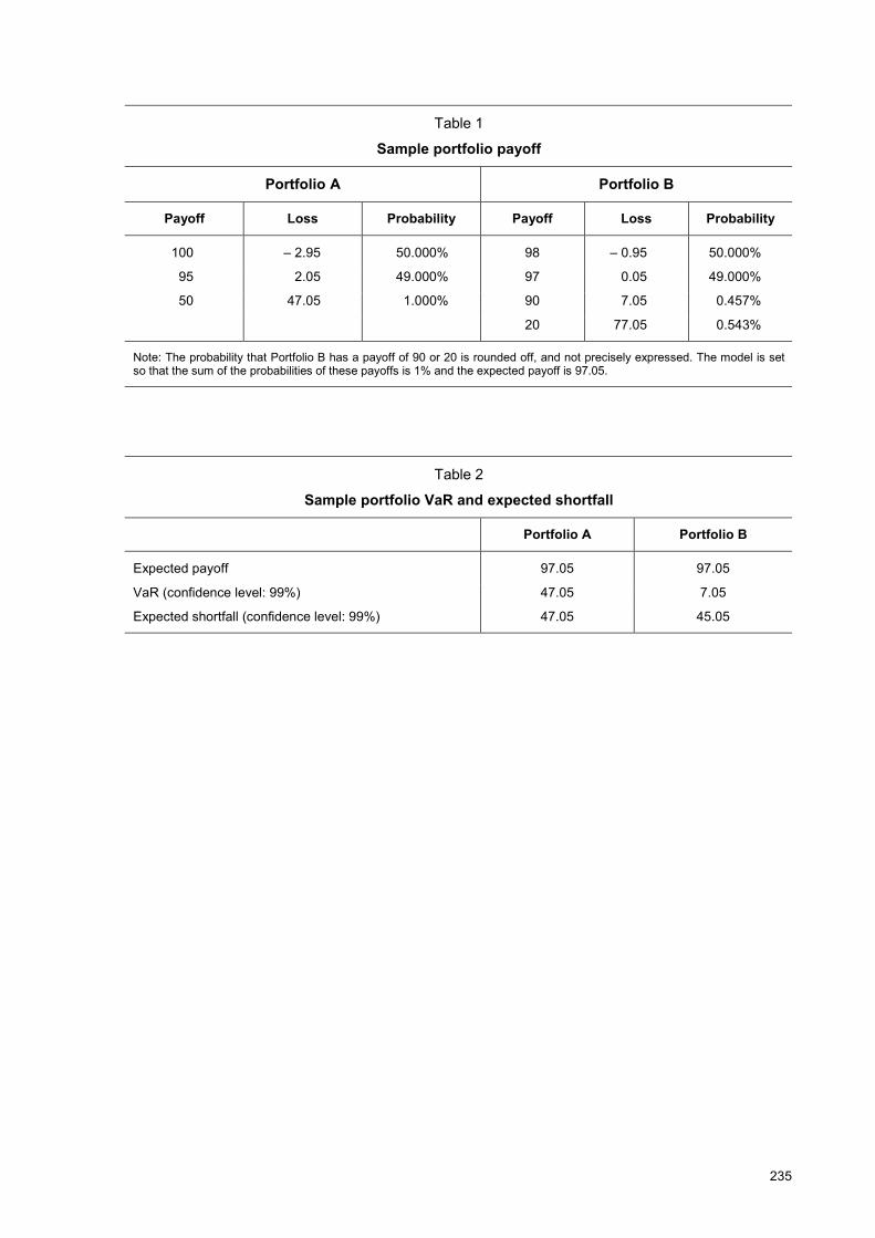

235

Table 1

Sample portfolio payoff

Portfolio A Portfolio B

Payoff Loss Probability Payoff Loss Probability

100 � 2.95 50.000% 98 � 0.95 50.000%

95 2.05 49.000% 97 0.05 49.000%

50 47.05 1.000% 90 7.05 0.457%

20 77.05 0.543%

Note: The probability that Portfolio B has a payoff of 90 or 20 is rounded off, and not precisely expressed. The model is set so that the sum of the probabilities of these payoffs is 1% and the expected payoff is 97.05.

Table 2

Sample portfolio VaR and expected shortfall

Portfolio A Portfolio B

Expected payoff 97.05 97.05

VaR (confidence level: 99%) 47.05 7.05

Expected shortfall (confidence level: 99%) 47.05 45.05

236

Figure 3

Distribution of exceedances with varied tail indices

0.9

0.91

0.92

0.93

0.94

0.95

0.96

0.97

0.98

0.99

1

0 1 2

Note: Where the tail probability is 1.0�p , the threshol

Distribution of exceed

0.9

0.91

0.92

0.93

0.94

0.95

0.96

0.97

0.98

0.99

1

0 1 2

Note: Where the tail probability is 1.0�p , the threshol

75.0��

0��

25.0��

1.0��

1��

�

5.0��

5.

3 4 5

d value is 0�� , and the scale parameter is 1�� .

Figure 4

ances with varied scale parameters

75.0�

3 4 5

d value is 0�� , and the tail index is 25.0�� .

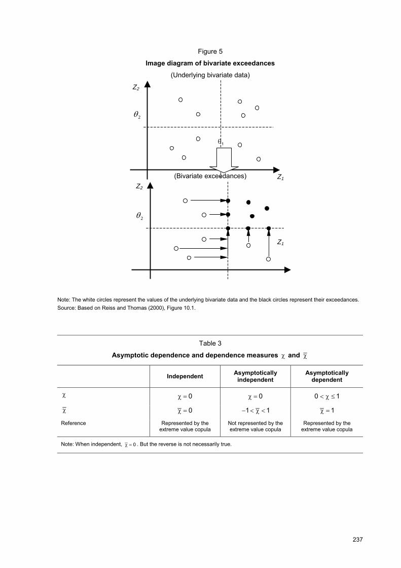
Figure 5

Image diagram of bivariate exceedances (Underlying bivariate data)

(Bivariate exc

Note: The white circles represent the values of the underlying bivaSource: Based on Reiss and Thomas (2000), Figure 10.1.

Table

Asymptotic dependence and de

Independent

� 0��

� 0��

Reference Represented by the extreme value copula

Note: When independent, 0�� . But the reverse is not necessa

Z2

1�

Z2

2�

2�

eedances) Z1

237

riate data and the black circles represent their exceedances.

3

pendence measures � and �

Asymptotically independent

Asymptotically dependent

0�� 10 ��

11 �� 1��

Not represented by the extreme value copula

Represented by the extreme value copula

rily true.

Z1

238

Table 4

Properties of the copulas used in this paper

Equation Dependence structure � �

Gumbel }])log()log[(exp{),( 1 ��

�� vuvuC Independent when 1��

Fully dependent when ��

�

��122 ( 1�� ) 1��

Gaussian ))(),((),( 11 vuvuC ��

��

Independent when 0��

Fully dependent when 1��

0�� )11( ��

Frank ��

��

�

�

��

��

��

��

eeeevuC

vu

1)1)(1(1ln1),(

Independent when 0��

Fully dependent when ��

0�� 0��

Figure 6

Example plot of the distribution of exceedances

0.9

0.95

1

0.05 0.1 0.15 0.2 0.25

Note: The tail probability is 1.021 �� pp and the threshold value is 05.021 �� .

s )( 1ZVaR)( 2ZVaR

Distribution function of 1Z ( 05.0,1.0 11 �� )

Distribution function of 2Z ( 035.0,5.0 22 �� )

Los

239

Table 5

Threshold value VaR� for the tail risk of VaR (Tail probability: p = 0.1, confidence level: 95%)

1�

0.10 0.20 0.30 0.40 0.50 0.60 0.70 0.80 0.90 1.00

0.10 � � � � � � � � � � 2� 0.20 1.036 � � � � � � � � �

0.30 1.073 1.036 � � � � � � � � 0.40 1.113 1.074 1.037 � � � � � � � 0.50 1.154 1.114 1.075 1.037 � � � � � � 0.60 1.198 1.156 1.116 1.076 1.038 � � � � � 0.70 1.243 1.200 1.158 1.117 1.077 1.038 � � � � 0.80 1.291 1.246 1.202 1.160 1.118 1.078 1.038 � � � 0.90 1.341 1.294 1.249 1.205 1.162 1.120 1.079 1.039 � � 1.00 1.393 1.345 1.298 1.252 1.207 1.163 1.121 1.079 1.039 �

(Tail probability: p = 0.1, confidence level: 99%)

1�

0.10 0.20 0.30 0.40 0.50 0.60 0.70 0.80 0.90 1.00

0.10 � � � � � � � � � � 2� 0.20 1.129 � � � � � � � � �

0.30 1.281 1.134 � � � � � � � � 0.40 1.460 1.292 1.139 � � � � � � � 0.50 1.670 1.479 1.304 1.144 � � � � � � 0.60 1.919 1.699 1.498 1.315 1.149 � � � � � 0.70 2.213 1.960 1.728 1.516 1.325 1.154 � � � � 0.80 2.563 2.269 2.001 1.756 1.535 1.336 1.158 � � � 0.90 2.980 2.638 2.325 2.041 1.784 1.553 1.346 1.162 � � 1.00 3.476 3.077 2.713 2.381 2.081 1.811 1.570 1.356 1.167 �


1�

0.10 0.20 0.30 0.40 0.50 0.60 0.70 0.80 0.90 1.00

0.10 � � � � � � � � � � 2� 0.20 1.087 � � � � � � � � �

0.30 1.185 1.090 � � � � � � � � 0.40 1.294 1.190 1.092 � � � � � � � 0.50 1.416 1.302 1.195 1.094 � � � � � � 0.60 1.552 1.428 1.310 1.200 1.097 � � � � � 0.70 1.706 1.569 1.440 1.319 1.205 1.099 � � � � 0.80 1.878 1.727 1.585 1.452 1.327 1.210 1.101 � � � 0.90 2.072 1.906 1.749 1.602 1.464 1.335 1.215 1.103 � � 1.00 2.291 2.107 1.933 1.771 1.618 1.476 1.343 1.220 1.105 �

Note: VaR has tail risk when 21 �� is more than VaR� .

240

Figure 7

Varied scale parameters and the tail risk of VaR

0.94

0.95

0.96

0.97

0.98

0.99

1

0.95

0.96

0.97

0.98

0.99

1

1,5.0 11 ��

0 1 2 3

Var

0 1

1,1.0 22 ��

5.1,1.0 22 ��

2,1.0 22 ��

1,1.0 11 ��

ied

2

4 5

Figure 8

tail indices and th

3

7.0,3.0 22 ��

,5.0 22 ��

2�

6 7 8 9 10

e tail risk of VaR

5

75.0�

75.0,9.0 2 ��

4 5 6

241

Table 6

Threshold value ES� for the tail risk of expected shortfall (Tail probability: 1.0�p , confidence level: 95%)

1�

0.10 0.20 0.30 0.40 0.50 0.60 0.70 0.80 0.90 1.00

0.10 � � � � � � � � � �2� 0.20 1.142 � � � � � � � � �

0.30 1.325 1.161 � � � � � � � � 0.40 1.571 1.376 1.185 � � � � � � � 0.50 1.916 1.678 1.446 1.220 � � � � � � 0.60 2.436 2.133 1.838 1.551 1.271 � � � � � 0.70 3.305 2.894 2.494 2.104 1.725 1.357 � � � � 0.80 5.047 4.420 3.808 3.213 2.634 2.072 1.527 � � � 0.90 10.281 9.004 7.758 6.545 5.366 4.221 3.111 2.037 � � 1.00 � � � � � � � � � �


1�

0.10 0.20 0.30 0.40 0.50 0.60 0.70 0.80 0.90 1.00

0.10 � � � � � � � � � �2� 0.20 1.230 � � � � � � � � �

0.30 1.547 1.257 � � � � � � � � 0.40 1.998 1.624 1.292 � � � � � � � 0.50 2.670 2.171 1.727 1.337 � � � � � � 0.60 3.741 3.042 2.419 1.873 1.401 � � � � � 0.70 5.626 4.574 3.638 2.817 2.107 1.504 � � � � 0.80 9.575 7.784 6.191 4.793 3.586 2.559 1.702 � � � 0.90 21.852 17.765 14.129 10.940 8.184 5.841 3.884 2.282 � � 1.00 � � � � � � � � � �


1�

0.10 0.20 0.30 0.40 0.50 0.60 0.70 0.80 0.90 1.00

0.10 � � � � � � � � � �2� 0.20 1.187 � � � � � � � � �

0.30 1.437 1.210 � � � � � � � � 0.40 1.780 1.499 1.239 � � � � � � � 0.50 2.276 1.917 1.584 1.278 � � � � � � 0.60 3.040 2.560 2.116 1.708 1.336 � � � � � 0.70 4.347 3.660 3.025 2.442 1.910 1.430 � � � � 0.80 7.013 5.906 4.881 3.940 3.082 2.307 1.613 � � � 0.90 15.136 12.747 10.535 8.503 6.651 4.978 3.482 2.158 � � 1.00 � � � � � � � � � �

Note: Expected shortfall has tail risk when 21 �� is more than ES� . When 1�� , we are unable to calculate expected shortfall as the first moment diverges.

242

Figure 9

Upward bias when using exceedances for risk measurement

The m

0

1

-3

1-p

Z2 Upward bias

2 4 6 8 10 12 14

��

0.1��

1.1��

0.2��

5.1��

Normal d

0.9

0.91

0.92

0.93

0.94

0.95

0.96

0.97

0.98

0.99

1

Figure 10

arginal distribution function assumed in this paper

0

Z1

Upward bias

istribution )(xF �� Distribution o

1(1��

�

1�

Exceedances
Non-exceedances
3

f exceedances )(xFF m�

)p

243

0.9

0.91

0.92

0.93

0.94

0.95

0.96

0.97

0.98

0.99

1

2 4 6 8 10 12 14

α = 1.0

α = 1.1

α = 1.5

α = 2.0

α = �

Figure 11

Empirical distribution functions of the sums under the Gumbel copula

Note: Empirical distributions are plotted from one million simulations with the marginal distribution parameters set at ,5.0�� ,1�� 1.0�p .

244

Table 7

VaR and expected shortfall under changes in the dependence parameter using a specific copula

Gumbel 1.0��

α VaR (95%) VaR (99%) VaR (99.9%) ES (95%) ES (99%) ES (99.9%)

1.0 2.971 5.165 8.748 4.357 6.715 10.670 1.1 3.150 5.777 10.724 4.852 7.915 13.702 1.2 3.299 6.252 11.822 5.189 8.623 14.974 1.3 3.412 6.563 12.429 5.425 9.071 15.676 1.4 3.505 6.798 12.861 5.597 9.374 16.117 1.5 3.577 6.980 13.111 5.725 9.586 16.410 1.6 3.634 7.087 13.295 5.822 9.740 16.615 1.7 3.682 7.178 13.417 5.898 9.857 16.767 1.8 3.718 7.247 13.485 5.958 9.948 16.886 1.9 3.748 7.307 13.547 6.007 10.020 16.983 2.0 3.772 7.357 13.602 6.048 10.078 17.060 5.0 3.957 7.672 13.966 6.311 10.417 17.561 10.0 3.981 7.694 14.033 6.342 10.456 17.595 � 3.993 7.703 14.219 6.352 10.502 17.613

Gaussian 1.0��

ρ VaR (95%) VaR (99%) VaR (99.9%) ES (95%) ES (99%) ES (99.9%)

0 2.971 5.165 8.748 4.357 6.715 10.670 0.1 3.124 5.435 9.275 4.585 7.086 11.257 0.2 3.250 5.687 9.747 4.786 7.423 11.842 0.3 3.366 5.932 10.262 4.986 7.770 12.473 0.4 3.476 6.180 10.798 5.183 8.129 13.159 0.5 3.576 6.424 11.324 5.380 8.505 13.891 0.6 3.671 6.671 11.939 5.577 8.898 14.663 0.7 3.761 6.923 12.507 5.775 9.309 15.464 0.8 3.842 7.198 13.132 5.978 9.736 16.288 0.9 3.921 7.501 13.727 6.189 10.172 17.149 1 3.993 7.703 14.219 6.352 10.502 17.613

Frank 1.0��

� VaR (95%) VaR (99%) VaR (99.9%) ES (95%) ES (99%) ES (99.9%)

0 2.971 5.165 8.748 4.357 6.715 10.670 1 3.171 5.438 9.071 4.600 7.017 11.025 2 3.348 5.687 9.392 4.817 7.290 11.344 3 3.492 5.901 9.656 5.000 7.524 11.618 4 3.607 6.074 9.875 5.153 7.720 11.852 5 3.699 6.226 10.056 5.278 7.884 12.049 6 3.770 6.349 10.217 5.380 8.022 12.218 7 3.828 6.451 10.362 5.466 8.141 12.363 8 3.874 6.539 10.484 5.538 8.245 12.489 9 3.914 6.614 10.599 5.600 8.337 12.601 � 3.993 7.703 14.219 6.352 10.502 17.613

Note: VaR and expected shortfall are calculated from one million simulations for each copula with the marginal distribution parameters set at σ = 1, p = 0.1. The tail index values are shown in the upper left of each table.

245

Table 7 (cont)

Gumbel 25.0��


1.0 3.125 6.065 12.465 5.083 8.858 17.463 1.1 3.302 6.694 14.824 5.595 10.170 21.106 1.2 3.437 7.162 16.085 5.949 10.994 23.018 1.3 3.543 7.501 16.986 6.200 11.538 24.174 1.4 3.628 7.745 17.557 6.384 11.920 24.944 1.5 3.696 7.920 18.004 6.521 12.195 25.479 1.6 3.750 8.049 18.214 6.626 12.398 25.863 1.7 3.792 8.152 18.429 6.708 12.554 26.154 1.8 3.827 8.231 18.594 6.773 12.675 26.383 1.9 3.852 8.284 18.652 6.827 12.773 26.568 2.0 3.874 8.339 18.732 6.871 12.852 26.718 5.0 4.036 8.699 19.286 7.159 13.330 27.802 10.0 4.059 8.726 19.414 7.194 13.388 27.911 � 4.071 8.735 19.778 7.206 13.454 27.837

Gaussian 25.0��


0 3.125 6.065 12.465 5.083 8.858 17.463 0.1 3.288 6.354 13.068 5.330 9.284 18.200 0.2 3.412 6.618 13.669 5.542 9.657 18.876 0.3 3.529 6.886 14.259 5.753 10.051 19.682 0.4 3.635 7.152 14.947 5.964 10.468 20.593 0.5 3.730 7.412 15.689 6.176 10.914 21.629 0.6 3.819 7.667 16.531 6.388 11.395 22.804 0.7 3.900 7.938 17.371 6.602 11.913 24.111 0.8 3.967 8.218 18.229 6.822 12.469 25.539 0.9 4.027 8.541 19.083 7.052 13.058 27.123 1 4.071 8.735 19.778 7.206 13.454 27.837

Frank 25.0��


0 3.125 6.065 12.465 5.083 8.858 17.463 1 3.328 6.345 12.869 5.335 9.180 17.847 2 3.506 6.608 13.170 5.561 9.478 18.210 3 3.654 6.847 13.453 5.755 9.739 18.531 4 3.770 7.034 13.740 5.916 9.960 18.803 5 3.863 7.202 14.000 6.050 10.145 19.037 6 3.935 7.340 14.168 6.159 10.302 19.237 7 3.991 7.451 14.308 6.250 10.437 19.409 8 4.035 7.554 14.468 6.328 10.556 19.566 9 4.071 7.641 14.598 6.394 10.662 19.705 � 4.071 8.735 19.778 7.206 13.454 27.837


246

Table 7 (cont)

Gumbel 5.0��


1.0 3.442 8.441 27.131 7.419 17.092 53.729 1.1 3.595 9.024 30.316 7.929 18.507 57.999 1.2 3.715 9.501 31.524 8.310 19.550 61.639 1.3 3.800 9.850 32.876 8.585 20.293 64.136 1.4 3.873 10.078 34.013 8.789 20.839 65.995 1.5 3.927 10.268 34.691 8.942 21.249 67.384 1.6 3.972 10.398 35.156 9.060 21.563 68.453 1.7 4.005 10.501 35.501 9.153 21.811 69.273 1.8 4.033 10.576 35.800 9.229 22.007 69.936 1.9 4.051 10.632 35.911 9.290 22.168 70.512 2.0 4.068 10.682 36.003 9.341 22.301 70.991 5.0 4.186 11.084 36.846 9.701 23.260 75.714 10.0 4.203 11.106 37.187 9.759 23.447 76.842 � 4.213 11.115 38.301 9.755 23.448 75.100

Gaussian 5.0��


0 3.442 8.441 27.131 7.419 17.092 53.729 0.1 3.615 8.803 28.052 7.728 17.747 55.729 0.2 3.739 9.077 28.675 7.968 18.231 57.090 0.3 3.851 9.379 29.438 8.209 18.763 58.693 0.4 3.949 9.679 30.552 8.451 19.337 60.525 0.5 4.037 9.943 31.695 8.693 19.947 62.477 0.6 4.106 10.216 32.864 8.934 20.614 64.683 0.7 4.167 10.481 34.683 9.176 21.358 67.279 0.8 4.207 10.753 36.224 9.425 22.204 70.588 0.9 4.230 11.062 37.467 9.691 23.159 74.816 1 4.213 11.115 38.301 9.755 23.448 75.100

Frank 5.0��


0 3.442 8.441 27.131 7.419 17.092 53.729 1 3.643 8.751 27.474 7.686 17.449 54.247 2 3.821 9.042 27.927 7.930 17.793 54.692 3 3.973 9.299 28.258 8.141 18.105 55.133 4 4.093 9.521 28.649 8.318 18.375 55.491 5 4.185 9.691 29.054 8.465 18.601 55.791 6 4.255 9.861 29.387 8.587 18.792 56.074 7 4.308 10.004 29.730 8.688 18.955 56.312 8 4.351 10.110 29.853 8.774 19.101 56.522 9 4.382 10.212 29.870 8.847 19.233 56.723 � 4.213 11.115 38.301 9.755 23.448 75.100


247

Table 7 (cont)

Gumbel 75.0��


1.0 3.847 12.654 68.724 14.106 45.232 232.931 1.1 3.961 13.076 73.107 14.193 44.817 220.165 1.2 4.054 13.468 74.485 14.574 46.065 226.977 1.3 4.117 13.752 74.705 14.878 47.107 232.902 1.4 4.167 13.980 75.957 15.110 47.934 237.781 1.5 4.209 14.130 78.154 15.288 48.578 241.740 1.6 4.243 14.277 77.773 15.427 49.087 244.924 1.7 4.263 14.314 78.758 15.540 49.504 247.554 1.8 4.278 14.362 79.165 15.633 49.861 249.744 1.9 4.291 14.373 79.241 15.713 50.164 251.761 2.0 4.302 14.380 78.839 15.781 50.431 253.590 5.0 4.355 14.716 78.988 16.542 53.710 282.245 10.0 4.364 14.714 80.040 16.844 55.155 295.725 � 4.373 14.720 83.395 16.517 53.579 275.707

Gaussian 75.0��


0 3.847 12.654 68.724 14.106 45.232 232.931 0.1 4.026 13.186 70.836 14.668 47.050 243.941 0.2 4.145 13.434 71.028 15.092 48.451 254.063 0.3 4.254 13.751 72.412 15.531 49.982 265.049 0.4 4.344 14.094 74.657 15.921 51.324 273.791 0.5 4.411 14.387 77.344 16.217 52.268 278.229 0.6 4.468 14.556 78.944 16.429 52.907 279.463 0.7 4.493 14.736 81.197 16.610 53.526 280.122 0.8 4.500 14.931 83.456 16.802 54.359 283.397 0.9 4.468 15.092 84.647 17.040 55.548 291.229 1 4.373 14.720 83.395 16.517 53.579 275.707

Frank 75.0��


0 3.847 12.654 68.724 14.106 45.232 232.931 1 4.051 12.988 68.816 14.397 45.680 234.046 2 4.229 13.318 69.598 14.665 46.116 234.846 3 4.376 13.620 70.071 14.897 46.507 235.493 4 4.494 13.879 70.484 15.091 46.843 235.963 5 4.580 14.069 70.999 15.251 47.117 236.298 6 4.650 14.258 71.637 15.383 47.344 236.603 7 4.703 14.398 73.037 15.493 47.537 236.907 8 4.739 14.515 72.559 15.587 47.708 237.163 9 4.767 14.634 72.669 15.669 47.873 237.456 � 4.373 14.720 83.395 16.517 53.579 275.707


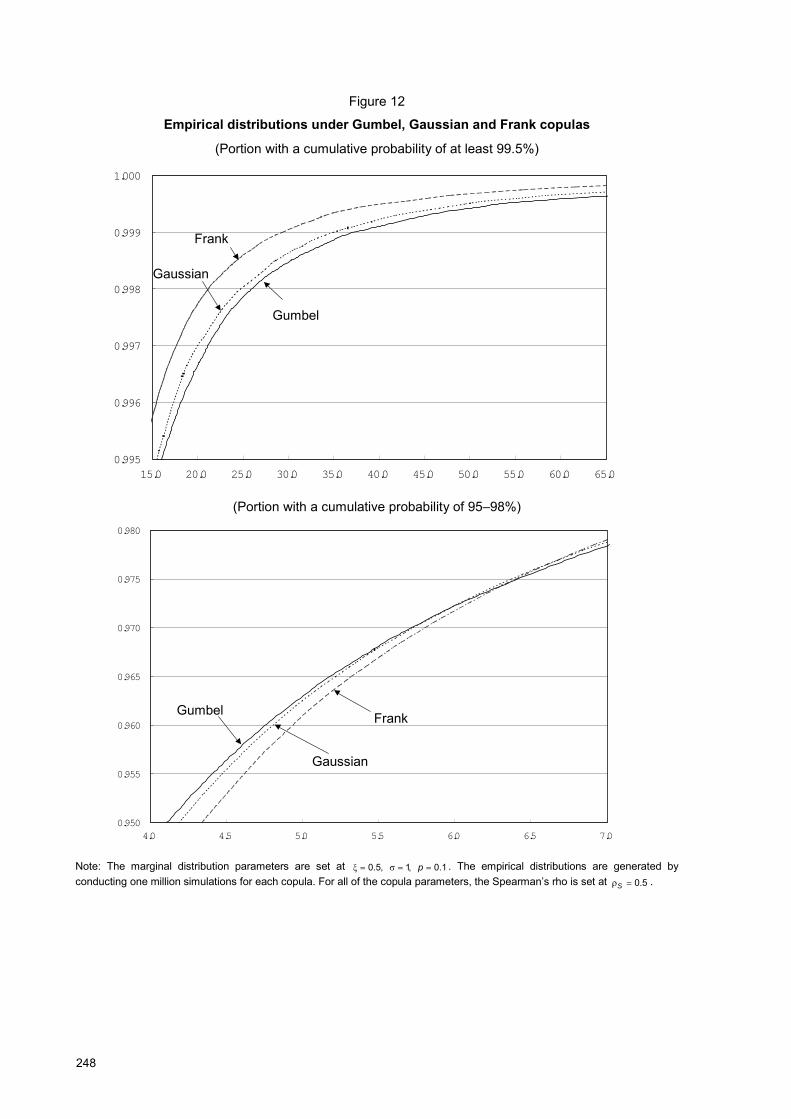
248

Figure 12

Empirical distributions under Gumbel, Gaussian and Frank copulas

(Portion with a cumulative probability of at least 99.5%)

0.995

0.996

0.997

0.998

0.999

1.000

15.0 20.0 25.0

(Portio

0.950

0.955

0.960

0.965

0.970

0.975

0.980

4.0 4.5

Note: The marginal distribution paramconducting one million simulations for ea

k

Gumbel

Fran

Gaussian

30.0 35.0 40.0 45.0 50.0 55.0 60.0 65.0

n with a cumulative probability of 95�98%)

Gumbel

5.0

eters are set at ��

ch copula. For all of t

k

n

Fran

Gaussia

5.5 6.0 6.5 7.0

1.0,1,5.0 �� p . The empirical distributions are generated by

he copula parameters, the Spearman�s rho is set at 5.0��S .

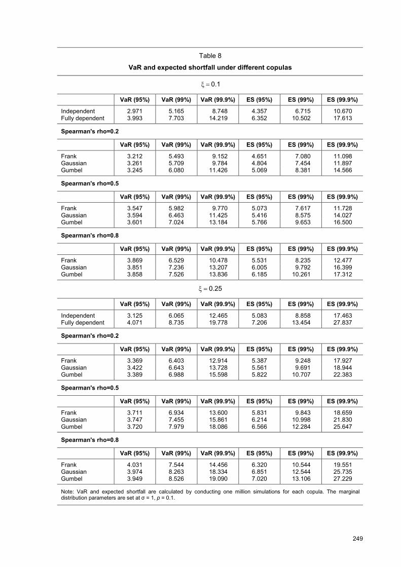
249

Table 8

VaR and expected shortfall under different copulas

1.0��

VaR (95%) VaR (99%) VaR (99.9%) ES (95%) ES (99%) ES (99.9%)

Independent 2.971 5.165 8.748 4.357 6.715 10.670 Fully dependent 3.993 7.703 14.219 6.352 10.502 17.613

Spearman's rho=0.2


Frank 3.212 5.493 9.152 4.651 7.080 11.098 Gaussian 3.261 5.709 9.784 4.804 7.454 11.897 Gumbel 3.245 6.080 11.426 5.069 8.381 14.566

Spearman's rho=0.5



Spearman's rho=0.8



25.0��



Spearman's rho=0.2



Spearman's rho=0.5



Spearman's rho=0.8



Note: VaR and expected shortfall are calculated by conducting one million simulations for each copula. The marginal distribution parameters are set at σ = 1, p = 0.1.

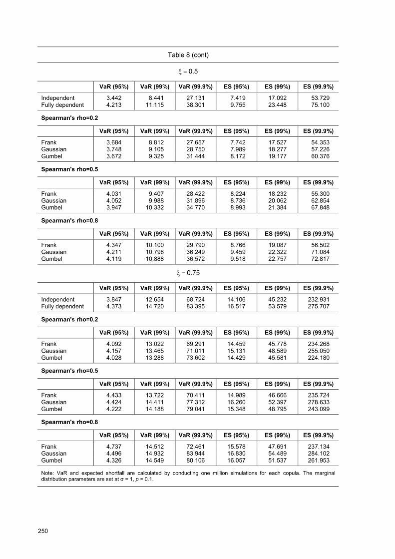
250

Table 8 (cont)

5.0��



Spearman's rho=0.2



Spearman's rho=0.5



Spearman's rho=0.8



75.0��



Spearman's rho=0.2



Spearman's rho=0.5



Spearman's rho=0.8



Note: VaR and expected shortfall are calculated by conducting one million simulations for each copula. The marginal distribution parameters are set at σ = 1, p = 0.1.

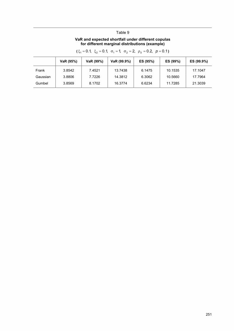
251

Table 9

VaR and expected shortfall under different copulas for different marginal distributions (example)

( 1.0,2.0,2,1,1.0,1.0 2121 �� pS )


Frank 3.8542 7.4521 13.7438 6.1475 10.1535 17.1047

Gaussian 3.8806 7.7226 14.3812 6.3062 10.5660 17.7964

Gumbel 3.8569 8.1702 16.3774 6.6234 11.7285 21.3039

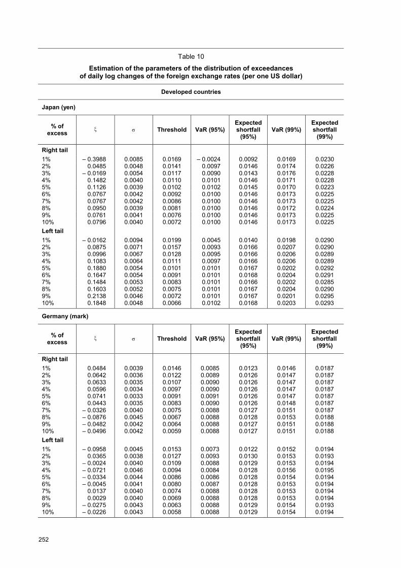
252

Table 10

Estimation of the parameters of the distribution of exceedances of daily log changes of the foreign exchange rates (per one US dollar)

Developed countries

Japan (yen)

% of excess

� � Threshold VaR (95%)

Expected shortfall

(95%) VaR (99%)

Expected shortfall

(99%)

Right tail 1% � 0.3988 0.0085 0.0169 � 0.0024 0.0092 0.0169 0.0230 2% 0.0485 0.0048 0.0141 0.0097 0.0146 0.0174 0.0226 3% � 0.0169 0.0054 0.0117 0.0090 0.0143 0.0176 0.0228 4% 0.1482 0.0040 0.0110 0.0101 0.0146 0.0171 0.0228 5% 0.1126 0.0039 0.0102 0.0102 0.0145 0.0170 0.0223 6% 0.0767 0.0042 0.0092 0.0100 0.0146 0.0173 0.0225 7% 0.0767 0.0042 0.0086 0.0100 0.0146 0.0173 0.0225 8% 0.0950 0.0039 0.0081 0.0100 0.0146 0.0172 0.0224 9% 0.0761 0.0041 0.0076 0.0100 0.0146 0.0173 0.0225 10% 0.0796 0.0040 0.0072 0.0100 0.0146 0.0173 0.0225 Left tail 1% � 0.0162 0.0094 0.0199 0.0045 0.0140 0.0198 0.0290 2% 0.0875 0.0071 0.0157 0.0093 0.0166 0.0207 0.0290 3% 0.0996 0.0067 0.0128 0.0095 0.0166 0.0206 0.0289 4% 0.1083 0.0064 0.0111 0.0097 0.0166 0.0206 0.0289 5% 0.1880 0.0054 0.0101 0.0101 0.0167 0.0202 0.0292 6% 0.1647 0.0054 0.0091 0.0101 0.0168 0.0204 0.0291 7% 0.1484 0.0053 0.0083 0.0101 0.0166 0.0202 0.0285 8% 0.1603 0.0052 0.0075 0.0101 0.0167 0.0204 0.0290 9% 0.2138 0.0046 0.0072 0.0101 0.0167 0.0201 0.0295 10% 0.1848 0.0048 0.0066 0.0102 0.0168 0.0203 0.0293

Germany (mark)

% of excess


Expected shortfall

(95%) VaR (99%)

Expected shortfall

(99%)

Right tail 1% 0.0484 0.0039 0.0146 0.0085 0.0123 0.0146 0.0187 2% 0.0642 0.0036 0.0122 0.0089 0.0126 0.0147 0.0187 3% 0.0633 0.0035 0.0107 0.0090 0.0126 0.0147 0.0187 4% 0.0596 0.0034 0.0097 0.0090 0.0126 0.0147 0.0187 5% 0.0741 0.0033 0.0091 0.0091 0.0126 0.0147 0.0187 6% 0.0443 0.0035 0.0083 0.0090 0.0126 0.0148 0.0187 7% � 0.0326 0.0040 0.0075 0.0088 0.0127 0.0151 0.0187 8% � 0.0876 0.0045 0.0067 0.0088 0.0128 0.0153 0.0188 9% � 0.0482 0.0042 0.0064 0.0088 0.0127 0.0151 0.0188 10% � 0.0496 0.0042 0.0059 0.0088 0.0127 0.0151 0.0188 Left tail 1% � 0.0958 0.0045 0.0153 0.0073 0.0122 0.0152 0.0194 2% 0.0365 0.0038 0.0127 0.0093 0.0130 0.0153 0.0193 3% � 0.0024 0.0040 0.0109 0.0088 0.0129 0.0153 0.0194 4% � 0.0721 0.0046 0.0094 0.0084 0.0128 0.0156 0.0195 5% � 0.0334 0.0044 0.0086 0.0086 0.0128 0.0154 0.0194 6% � 0.0045 0.0041 0.0080 0.0087 0.0128 0.0153 0.0194 7% 0.0137 0.0040 0.0074 0.0088 0.0128 0.0153 0.0194 8% 0.0029 0.0040 0.0069 0.0088 0.0128 0.0153 0.0194 9% � 0.0275 0.0043 0.0063 0.0088 0.0129 0.0154 0.0193 10% � 0.0226 0.0043 0.0058 0.0088 0.0129 0.0154 0.0194

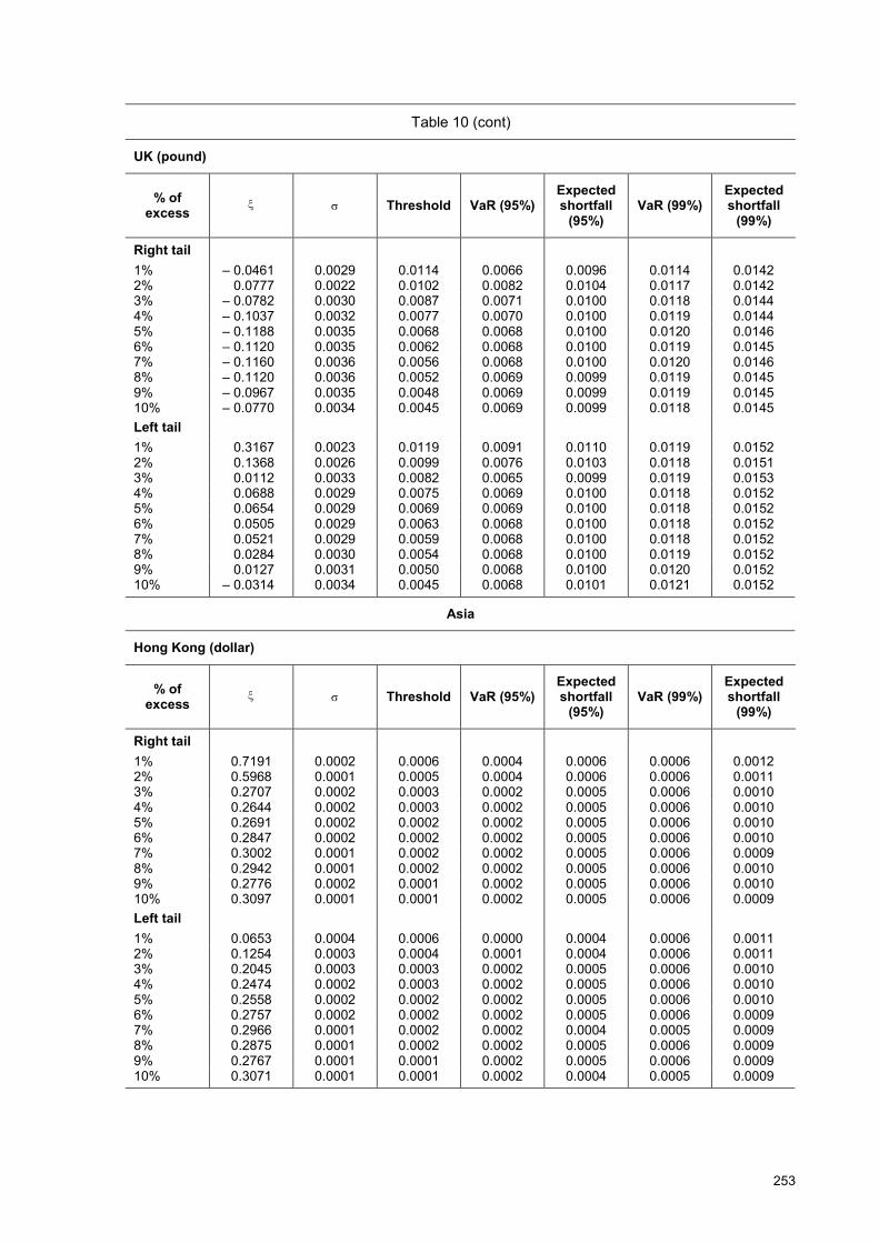
253

Table 10 (cont)

UK (pound)

% of excess


Expected shortfall

(95%) VaR (99%)

Expected shortfall

(99%)

Right tail 1% � 0.0461 0.0029 0.0114 0.0066 0.0096 0.0114 0.0142 2% 0.0777 0.0022 0.0102 0.0082 0.0104 0.0117 0.0142 3% � 0.0782 0.0030 0.0087 0.0071 0.0100 0.0118 0.0144 4% � 0.1037 0.0032 0.0077 0.0070 0.0100 0.0119 0.0144 5% � 0.1188 0.0035 0.0068 0.0068 0.0100 0.0120 0.0146 6% � 0.1120 0.0035 0.0062 0.0068 0.0100 0.0119 0.0145 7% � 0.1160 0.0036 0.0056 0.0068 0.0100 0.0120 0.0146 8% � 0.1120 0.0036 0.0052 0.0069 0.0099 0.0119 0.0145 9% � 0.0967 0.0035 0.0048 0.0069 0.0099 0.0119 0.0145 10% � 0.0770 0.0034 0.0045 0.0069 0.0099 0.0118 0.0145 Left tail 1% 0.3167 0.0023 0.0119 0.0091 0.0110 0.0119 0.0152 2% 0.1368 0.0026 0.0099 0.0076 0.0103 0.0118 0.0151 3% 0.0112 0.0033 0.0082 0.0065 0.0099 0.0119 0.0153 4% 0.0688 0.0029 0.0075 0.0069 0.0100 0.0118 0.0152 5% 0.0654 0.0029 0.0069 0.0069 0.0100 0.0118 0.0152 6% 0.0505 0.0029 0.0063 0.0068 0.0100 0.0118 0.0152 7% 0.0521 0.0029 0.0059 0.0068 0.0100 0.0118 0.0152 8% 0.0284 0.0030 0.0054 0.0068 0.0100 0.0119 0.0152 9% 0.0127 0.0031 0.0050 0.0068 0.0100 0.0120 0.0152 10% � 0.0314 0.0034 0.0045 0.0068 0.0101 0.0121 0.0152

Asia

Hong Kong (dollar)

% of excess


Expected shortfall

(95%) VaR (99%)

Expected shortfall

(99%)

Right tail 1% 0.7191 0.0002 0.0006 0.0004 0.0006 0.0006 0.0012 2% 0.5968 0.0001 0.0005 0.0004 0.0006 0.0006 0.0011 3% 0.2707 0.0002 0.0003 0.0002 0.0005 0.0006 0.0010 4% 0.2644 0.0002 0.0003 0.0002 0.0005 0.0006 0.0010 5% 0.2691 0.0002 0.0002 0.0002 0.0005 0.0006 0.0010 6% 0.2847 0.0002 0.0002 0.0002 0.0005 0.0006 0.0010 7% 0.3002 0.0001 0.0002 0.0002 0.0005 0.0006 0.0009 8% 0.2942 0.0001 0.0002 0.0002 0.0005 0.0006 0.0010 9% 0.2776 0.0002 0.0001 0.0002 0.0005 0.0006 0.0010 10% 0.3097 0.0001 0.0001 0.0002 0.0005 0.0006 0.0009 Left tail 1% 0.0653 0.0004 0.0006 0.0000 0.0004 0.0006 0.0011 2% 0.1254 0.0003 0.0004 0.0001 0.0004 0.0006 0.0011 3% 0.2045 0.0003 0.0003 0.0002 0.0005 0.0006 0.0010 4% 0.2474 0.0002 0.0003 0.0002 0.0005 0.0006 0.0010 5% 0.2558 0.0002 0.0002 0.0002 0.0005 0.0006 0.0010 6% 0.2757 0.0002 0.0002 0.0002 0.0005 0.0006 0.0009 7% 0.2966 0.0001 0.0002 0.0002 0.0004 0.0005 0.0009 8% 0.2875 0.0001 0.0002 0.0002 0.0005 0.0006 0.0009 9% 0.2767 0.0001 0.0001 0.0002 0.0005 0.0006 0.0009 10% 0.3071 0.0001 0.0001 0.0002 0.0004 0.0005 0.0009

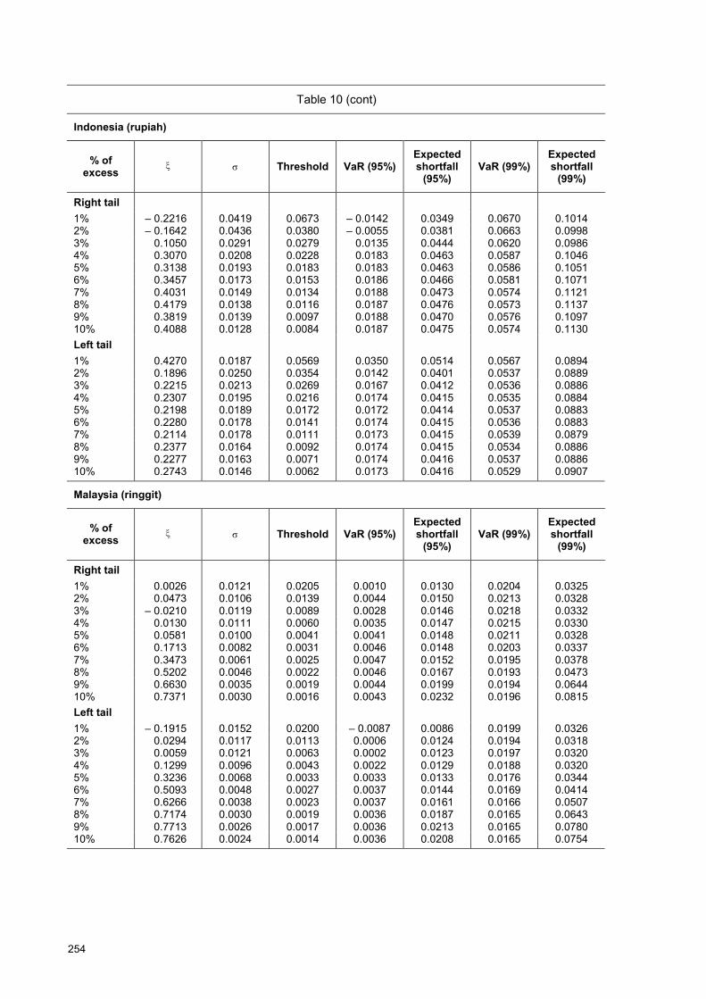
254

Table 10 (cont)

Indonesia (rupiah)

% of excess


Expected shortfall

(95%) VaR (99%)

Expected shortfall

(99%)

Right tail 1% � 0.2216 0.0419 0.0673 � 0.0142 0.0349 0.0670 0.1014 2% � 0.1642 0.0436 0.0380 � 0.0055 0.0381 0.0663 0.0998 3% 0.1050 0.0291 0.0279 0.0135 0.0444 0.0620 0.0986 4% 0.3070 0.0208 0.0228 0.0183 0.0463 0.0587 0.1046 5% 0.3138 0.0193 0.0183 0.0183 0.0463 0.0586 0.1051 6% 0.3457 0.0173 0.0153 0.0186 0.0466 0.0581 0.1071 7% 0.4031 0.0149 0.0134 0.0188 0.0473 0.0574 0.1121 8% 0.4179 0.0138 0.0116 0.0187 0.0476 0.0573 0.1137 9% 0.3819 0.0139 0.0097 0.0188 0.0470 0.0576 0.1097 10% 0.4088 0.0128 0.0084 0.0187 0.0475 0.0574 0.1130 Left tail 1% 0.4270 0.0187 0.0569 0.0350 0.0514 0.0567 0.0894 2% 0.1896 0.0250 0.0354 0.0142 0.0401 0.0537 0.0889 3% 0.2215 0.0213 0.0269 0.0167 0.0412 0.0536 0.0886 4% 0.2307 0.0195 0.0216 0.0174 0.0415 0.0535 0.0884 5% 0.2198 0.0189 0.0172 0.0172 0.0414 0.0537 0.0883 6% 0.2280 0.0178 0.0141 0.0174 0.0415 0.0536 0.0883 7% 0.2114 0.0178 0.0111 0.0173 0.0415 0.0539 0.0879 8% 0.2377 0.0164 0.0092 0.0174 0.0415 0.0534 0.0886 9% 0.2277 0.0163 0.0071 0.0174 0.0416 0.0537 0.0886 10% 0.2743 0.0146 0.0062 0.0173 0.0416 0.0529 0.0907

Malaysia (ringgit)

% of excess


Expected shortfall

(95%) VaR (99%)

Expected shortfall

(99%)

Right tail 1% 0.0026 0.0121 0.0205 0.0010 0.0130 0.0204 0.0325 2% 0.0473 0.0106 0.0139 0.0044 0.0150 0.0213 0.0328 3% � 0.0210 0.0119 0.0089 0.0028 0.0146 0.0218 0.0332 4% 0.0130 0.0111 0.0060 0.0035 0.0147 0.0215 0.0330 5% 0.0581 0.0100 0.0041 0.0041 0.0148 0.0211 0.0328 6% 0.1713 0.0082 0.0031 0.0046 0.0148 0.0203 0.0337 7% 0.3473 0.0061 0.0025 0.0047 0.0152 0.0195 0.0378 8% 0.5202 0.0046 0.0022 0.0046 0.0167 0.0193 0.0473 9% 0.6630 0.0035 0.0019 0.0044 0.0199 0.0194 0.0644 10% 0.7371 0.0030 0.0016 0.0043 0.0232 0.0196 0.0815 Left tail 1% � 0.1915 0.0152 0.0200 � 0.0087 0.0086 0.0199 0.0326 2% 0.0294 0.0117 0.0113 0.0006 0.0124 0.0194 0.0318 3% 0.0059 0.0121 0.0063 0.0002 0.0123 0.0197 0.0320 4% 0.1299 0.0096 0.0043 0.0022 0.0129 0.0188 0.0320 5% 0.3236 0.0068 0.0033 0.0033 0.0133 0.0176 0.0344 6% 0.5093 0.0048 0.0027 0.0037 0.0144 0.0169 0.0414 7% 0.6266 0.0038 0.0023 0.0037 0.0161 0.0166 0.0507 8% 0.7174 0.0030 0.0019 0.0036 0.0187 0.0165 0.0643 9% 0.7713 0.0026 0.0017 0.0036 0.0213 0.0165 0.0780 10% 0.7626 0.0024 0.0014 0.0036 0.0208 0.0165 0.0754

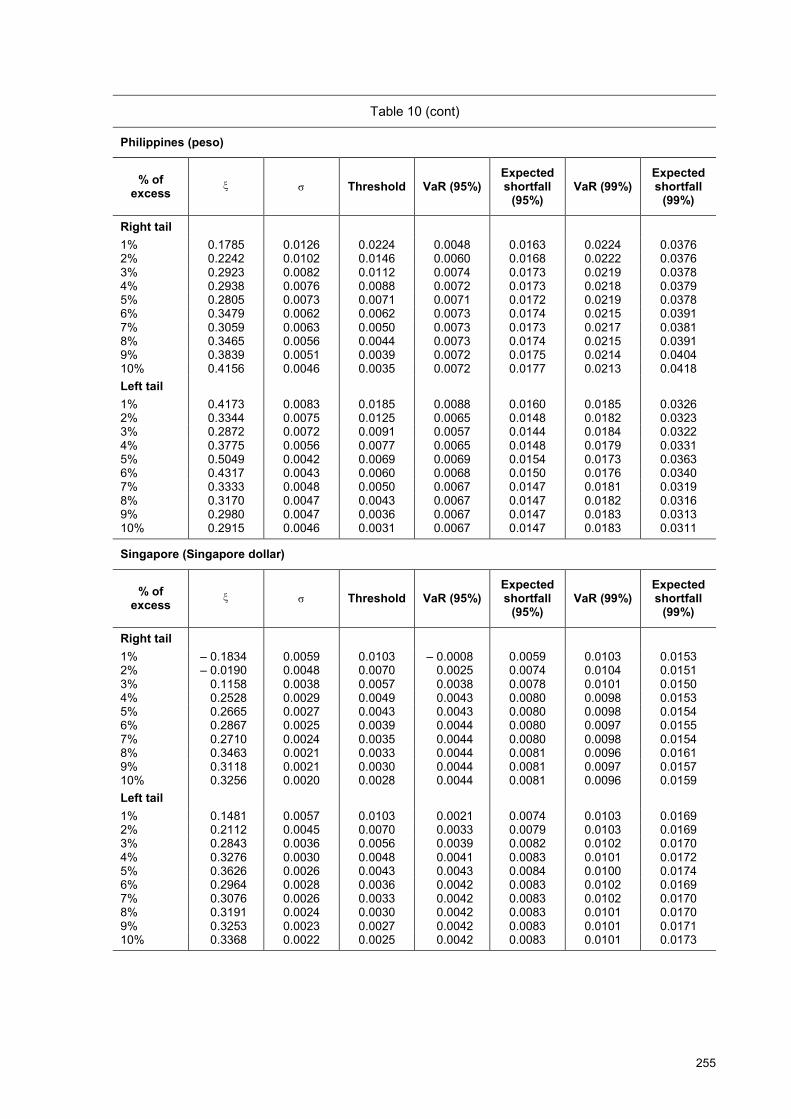
255

Table 10 (cont)

Philippines (peso)

% of excess


Expected shortfall

(95%) VaR (99%)

Expected shortfall

(99%)


Singapore (Singapore dollar)

% of excess


Expected shortfall

(95%) VaR (99%)

Expected shortfall

(99%)

Right tail 1% � 0.1834 0.0059 0.0103 � 0.0008 0.0059 0.0103 0.0153 2% � 0.0190 0.0048 0.0070 0.0025 0.0074 0.0104 0.0151 3% 0.1158 0.0038 0.0057 0.0038 0.0078 0.0101 0.0150 4% 0.2528 0.0029 0.0049 0.0043 0.0080 0.0098 0.0153 5% 0.2665 0.0027 0.0043 0.0043 0.0080 0.0098 0.0154 6% 0.2867 0.0025 0.0039 0.0044 0.0080 0.0097 0.0155 7% 0.2710 0.0024 0.0035 0.0044 0.0080 0.0098 0.0154 8% 0.3463 0.0021 0.0033 0.0044 0.0081 0.0096 0.0161 9% 0.3118 0.0021 0.0030 0.0044 0.0081 0.0097 0.0157 10% 0.3256 0.0020 0.0028 0.0044 0.0081 0.0096 0.0159 Left tail 1% 0.1481 0.0057 0.0103 0.0021 0.0074 0.0103 0.0169 2% 0.2112 0.0045 0.0070 0.0033 0.0079 0.0103 0.0169 3% 0.2843 0.0036 0.0056 0.0039 0.0082 0.0102 0.0170 4% 0.3276 0.0030 0.0048 0.0041 0.0083 0.0101 0.0172 5% 0.3626 0.0026 0.0043 0.0043 0.0084 0.0100 0.0174 6% 0.2964 0.0028 0.0036 0.0042 0.0083 0.0102 0.0169 7% 0.3076 0.0026 0.0033 0.0042 0.0083 0.0102 0.0170 8% 0.3191 0.0024 0.0030 0.0042 0.0083 0.0101 0.0170 9% 0.3253 0.0023 0.0027 0.0042 0.0083 0.0101 0.0171 10% 0.3368 0.0022 0.0025 0.0042 0.0083 0.0101 0.0173

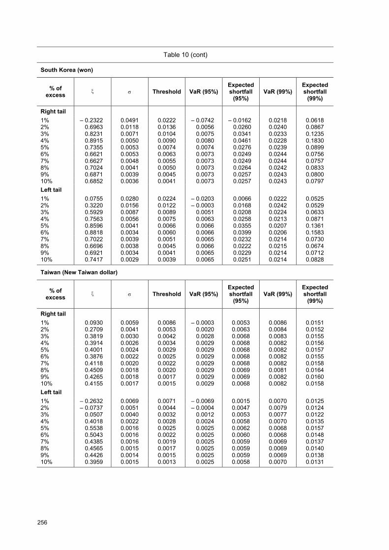
256

Table 10 (cont)

South Korea (won)

% of excess


Expected shortfall

(95%) VaR (99%)

Expected shortfall

(99%)

Right tail 1% � 0.2322 0.0491 0.0222 � 0.0742 � 0.0162 0.0218 0.0618 2% 0.6963 0.0118 0.0136 0.0056 0.0260 0.0240 0.0867 3% 0.8231 0.0071 0.0104 0.0075 0.0341 0.0233 0.1235 4% 0.8915 0.0050 0.0090 0.0080 0.0461 0.0228 0.1830 5% 0.7355 0.0053 0.0074 0.0074 0.0276 0.0239 0.0899 6% 0.6621 0.0053 0.0063 0.0073 0.0249 0.0244 0.0756 7% 0.6627 0.0048 0.0055 0.0073 0.0249 0.0244 0.0757 8% 0.7024 0.0041 0.0050 0.0073 0.0264 0.0242 0.0833 9% 0.6871 0.0039 0.0045 0.0073 0.0257 0.0243 0.0800 10% 0.6852 0.0036 0.0041 0.0073 0.0257 0.0243 0.0797 Left tail 1% 0.0755 0.0280 0.0224 � 0.0203 0.0066 0.0222 0.0525 2% 0.3220 0.0156 0.0122 � 0.0003 0.0168 0.0242 0.0529 3% 0.5929 0.0087 0.0089 0.0051 0.0208 0.0224 0.0633 4% 0.7563 0.0056 0.0075 0.0063 0.0258 0.0213 0.0871 5% 0.8596 0.0041 0.0066 0.0066 0.0355 0.0207 0.1361 6% 0.8818 0.0034 0.0060 0.0066 0.0399 0.0206 0.1583 7% 0.7022 0.0039 0.0051 0.0065 0.0232 0.0214 0.0730 8% 0.6696 0.0038 0.0045 0.0066 0.0222 0.0215 0.0674 9% 0.6921 0.0034 0.0041 0.0065 0.0229 0.0214 0.0712 10% 0.7417 0.0029 0.0039 0.0065 0.0251 0.0214 0.0828

Taiwan (New Taiwan dollar)

% of excess


Expected shortfall

(95%) VaR (99%)

Expected shortfall

(99%)

Right tail 1% 0.0930 0.0059 0.0086 � 0.0003 0.0053 0.0086 0.0151 2% 0.2709 0.0041 0.0053 0.0020 0.0063 0.0084 0.0152 3% 0.3819 0.0030 0.0042 0.0028 0.0068 0.0083 0.0155 4% 0.3914 0.0026 0.0034 0.0029 0.0068 0.0082 0.0156 5% 0.4001 0.0024 0.0029 0.0029 0.0068 0.0082 0.0157 6% 0.3876 0.0022 0.0025 0.0029 0.0068 0.0082 0.0155 7% 0.4118 0.0020 0.0022 0.0029 0.0068 0.0082 0.0158 8% 0.4509 0.0018 0.0020 0.0029 0.0069 0.0081 0.0164 9% 0.4265 0.0018 0.0017 0.0029 0.0069 0.0082 0.0160 10% 0.4155 0.0017 0.0015 0.0029 0.0068 0.0082 0.0158 Left tail 1% � 0.2632 0.0069 0.0071 � 0.0069 0.0015 0.0070 0.0125 2% � 0.0737 0.0051 0.0044 � 0.0004 0.0047 0.0079 0.0124 3% 0.0507 0.0040 0.0032 0.0012 0.0053 0.0077 0.0122 4% 0.4018 0.0022 0.0028 0.0024 0.0058 0.0070 0.0135 5% 0.5538 0.0016 0.0025 0.0025 0.0062 0.0068 0.0157 6% 0.5043 0.0016 0.0022 0.0025 0.0060 0.0068 0.0148 7% 0.4385 0.0016 0.0019 0.0025 0.0059 0.0069 0.0137 8% 0.4565 0.0015 0.0017 0.0025 0.0059 0.0069 0.0140 9% 0.4426 0.0014 0.0015 0.0025 0.0059 0.0069 0.0138 10% 0.3959 0.0015 0.0013 0.0025 0.0058 0.0070 0.0131

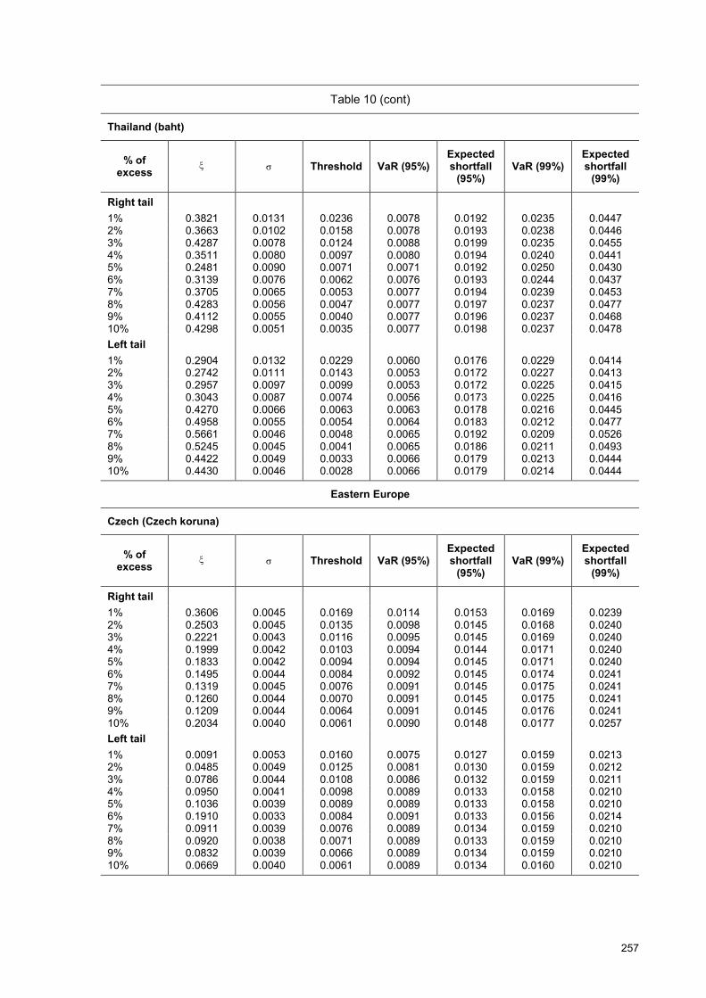
257

Table 10 (cont)

Thailand (baht)

% of excess


Expected shortfall

(95%) VaR (99%)

Expected shortfall

(99%)


Eastern Europe

Czech (Czech koruna)

% of excess


Expected shortfall

(95%) VaR (99%)

Expected shortfall

(99%)


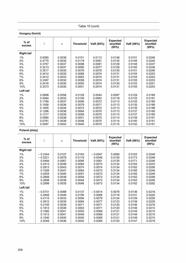
258

Table 10 (cont)

Hungary (forint)

% of excess


Expected shortfall

(95%) VaR (99%)

Expected shortfall

(99%)


Poland (zloty)

% of excess


Expected shortfall

(95%) VaR (99%)

Expected shortfall

(99%)

Right tail 1% � 0.2344 0.0107 0.0163 � 0.0047 0.0080 0.0163 0.0249 2% � 0.0221 0.0078 0.0119 0.0046 0.0125 0.0173 0.0248 3% 0.0484 0.0067 0.0095 0.0061 0.0130 0.0171 0.0246 4% 0.2413 0.0048 0.0084 0.0073 0.0134 0.0163 0.0253 5% 0.2813 0.0043 0.0074 0.0074 0.0134 0.0162 0.0256 6% 0.1926 0.0047 0.0064 0.0073 0.0134 0.0165 0.0248 7% 0.2054 0.0045 0.0057 0.0073 0.0134 0.0165 0.0249 8% 0.2809 0.0038 0.0054 0.0073 0.0134 0.0162 0.0258 9% 0.2698 0.0038 0.0049 0.0073 0.0134 0.0163 0.0256 10% 0.2999 0.0035 0.0046 0.0073 0.0134 0.0162 0.0262 Left tail 1% � 0.0731 0.0088 0.0137 � 0.0014 0.0078 0.0136 0.0218 2% 0.2848 0.0046 0.0106 0.0068 0.0118 0.0141 0.0220 3% 0.4115 0.0033 0.0094 0.0079 0.0124 0.0139 0.0226 4% 0.3912 0.0030 0.0084 0.0077 0.0123 0.0139 0.0225 5% 0.2105 0.0039 0.0071 0.0071 0.0120 0.0146 0.0216 6% 0.1813 0.0039 0.0063 0.0071 0.0120 0.0146 0.0212 7% 0.1560 0.0041 0.0055 0.0069 0.0121 0.0149 0.0214 8% 0.1513 0.0041 0.0049 0.0069 0.0121 0.0149 0.0215 9% 0.1540 0.0040 0.0045 0.0069 0.0121 0.0149 0.0215 10% 0.2049 0.0036 0.0042 0.0069 0.0120 0.0147 0.0219

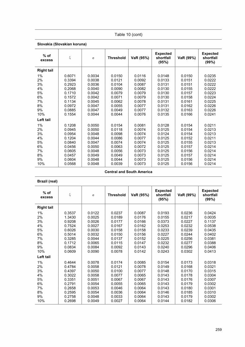
259

Table 10 (cont)

Slovakia (Slovakian koruna)

% of excess


Expected shortfall

(95%) VaR (99%)

Expected shortfall

(99%)


Central and South America

Brazil (real)

% of excess


Expected shortfall

(95%) VaR (99%)

Expected shortfall

(99%)


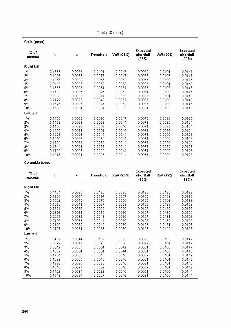
260

Table 10 (cont)

Chile (peso)

% of excess


Expected shortfall

(95%) VaR (99%)

Expected shortfall

(99%)


Columbia (peso)

% of excess


Expected shortfall

(95%) VaR (99%)

Expected shortfall

(99%)


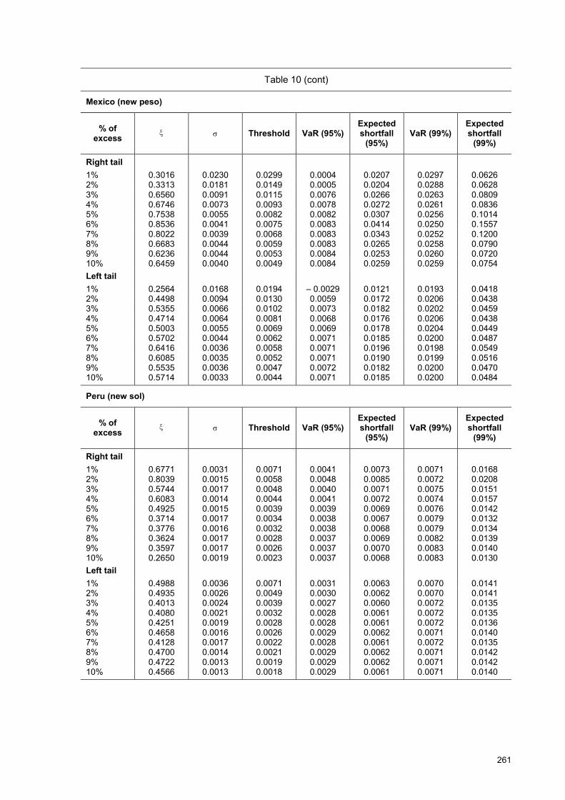
261

Table 10 (cont)

Mexico (new peso)

% of excess


Expected shortfall

(95%) VaR (99%)

Expected shortfall

(99%)

Right tail 1% 0.3016 0.0230 0.0299 0.0004 0.0207 0.0297 0.0626 2% 0.3313 0.0181 0.0149 0.0005 0.0204 0.0288 0.0628 3% 0.6560 0.0091 0.0115 0.0076 0.0266 0.0263 0.0809 4% 0.6746 0.0073 0.0093 0.0078 0.0272 0.0261 0.0836 5% 0.7538 0.0055 0.0082 0.0082 0.0307 0.0256 0.1014 6% 0.8536 0.0041 0.0075 0.0083 0.0414 0.0250 0.1557 7% 0.8022 0.0039 0.0068 0.0083 0.0343 0.0252 0.1200 8% 0.6683 0.0044 0.0059 0.0083 0.0265 0.0258 0.0790 9% 0.6236 0.0044 0.0053 0.0084 0.0253 0.0260 0.0720 10% 0.6459 0.0040 0.0049 0.0084 0.0259 0.0259 0.0754 Left tail 1% 0.2564 0.0168 0.0194 � 0.0029 0.0121 0.0193 0.0418 2% 0.4498 0.0094 0.0130 0.0059 0.0172 0.0206 0.0438 3% 0.5355 0.0066 0.0102 0.0073 0.0182 0.0202 0.0459 4% 0.4714 0.0064 0.0081 0.0068 0.0176 0.0206 0.0438 5% 0.5003 0.0055 0.0069 0.0069 0.0178 0.0204 0.0449 6% 0.5702 0.0044 0.0062 0.0071 0.0185 0.0200 0.0487 7% 0.6416 0.0036 0.0058 0.0071 0.0196 0.0198 0.0549 8% 0.6085 0.0035 0.0052 0.0071 0.0190 0.0199 0.0516 9% 0.5535 0.0036 0.0047 0.0072 0.0182 0.0200 0.0470 10% 0.5714 0.0033 0.0044 0.0071 0.0185 0.0200 0.0484

Peru (new sol)

% of excess


Expected shortfall

(95%) VaR (99%)

Expected shortfall

(99%)


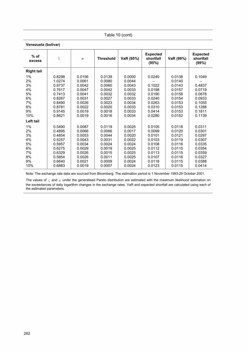
262

Table 10 (cont)

Venezuela (bolívar)

% of excess


Expected shortfall

(95%) VaR (99%)

Expected shortfall

(99%)

Right tail 1% 0.8298 0.0156 0.0139 0.0000 0.0240 0.0138 0.1049 2% 1.0274 0.0061 0.0080 0.0044 � 0.0140 � 3% 0.9737 0.0042 0.0060 0.0043 0.1022 0.0143 0.4837 4% 0.7617 0.0047 0.0042 0.0033 0.0198 0.0157 0.0719 5% 0.7413 0.0041 0.0032 0.0032 0.0190 0.0158 0.0678 6% 0.8267 0.0031 0.0027 0.0033 0.0240 0.0154 0.0933 7% 0.8490 0.0026 0.0023 0.0034 0.0263 0.0153 0.1055 8% 0.8781 0.0022 0.0020 0.0033 0.0310 0.0153 0.1288 9% 0.9145 0.0019 0.0018 0.0033 0.0414 0.0153 0.1811 10% 0.8621 0.0019 0.0016 0.0034 0.0280 0.0152 0.1139 Left tail 1% 0.5490 0.0087 0.0119 0.0025 0.0105 0.0118 0.0311 2% 0.4895 0.0066 0.0066 0.0017 0.0099 0.0120 0.0301 3% 0.4854 0.0053 0.0044 0.0020 0.0101 0.0121 0.0297 4% 0.5257 0.0043 0.0031 0.0022 0.0103 0.0119 0.0307 5% 0.5957 0.0034 0.0024 0.0024 0.0108 0.0116 0.0335 6% 0.6275 0.0029 0.0019 0.0025 0.0112 0.0115 0.0354 7% 0.6329 0.0026 0.0015 0.0025 0.0113 0.0115 0.0359 8% 0.5854 0.0026 0.0011 0.0025 0.0107 0.0116 0.0327 9% 0.6640 0.0021 0.0009 0.0024 0.0118 0.0115 0.0388 10% 0.6883 0.0019 0.0007 0.0024 0.0123 0.0115 0.0414

Note: The exchange rate data are sourced from Bloomberg. The estimation period is 1 November 1993-29 October 2001.

The values of � and � under the generalised Pareto distribution are estimated with the maximum likelihood estimation on the exceedances of daily logarithm changes in the exchange rates. VaR and expected shortfall are calculated using each of the estimated parameters.

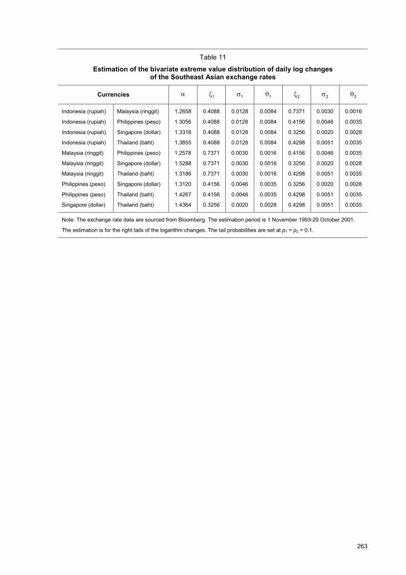
263

Table 11

Estimation of the bivariate extreme value distribution of daily log changes of the Southeast Asian exchange rates

Currencies � 1� 1� 1� 2� 2� 2�

Indonesia (rupiah) Malaysia (ringgit) 1.2658 0.4088 0.0128 0.0084 0.7371 0.0030 0.0016

Indonesia (rupiah) Philippines (peso) 1.3056 0.4088 0.0128 0.0084 0.4156 0.0046 0.0035

Indonesia (rupiah) Singapore (dollar) 1.3316 0.4088 0.0128 0.0084 0.3256 0.0020 0.0028

Indonesia (rupiah) Thailand (baht) 1.3855 0.4088 0.0128 0.0084 0.4298 0.0051 0.0035

Malaysia (ringgit) Philippines (peso) 1.2578 0.7371 0.0030 0.0016 0.4156 0.0046 0.0035

Malaysia (ringgit) Singapore (dollar) 1.5288 0.7371 0.0030 0.0016 0.3256 0.0020 0.0028

Malaysia (ringgit) Thailand (baht) 1.3186 0.7371 0.0030 0.0016 0.4298 0.0051 0.0035

Philippines (peso) Singapore (dollar) 1.3120 0.4156 0.0046 0.0035 0.3256 0.0020 0.0028

Philippines (peso) Thailand (baht) 1.4267 0.4156 0.0046 0.0035 0.4298 0.0051 0.0035

Singapore (dollar) Thailand (baht) 1.4364 0.3256 0.0020 0.0028 0.4298 0.0051 0.0035

Note: The exchange rate data are sourced from Bloomberg. The estimation period is 1 November 1993-29 October 2001.

The estimation is for the right tails of the logarithm changes. The tail probabilities are set at p1 = p2 = 0.1.

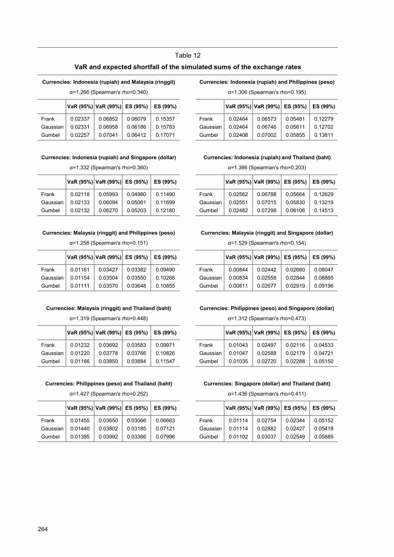
264

Table 12

VaR and expected shortfall of the simulated sums of the exchange rates

Currencies: Indonesia (rupiah) and Malaysia (ringgit) Currencies: Indonesia (rupiah) and Philippines (peso)

α=1.266 (Spearman's rho=0.340) α=1.306 (Spearman's rho=0.195)

VaR (95%) VaR (99%) ES (95%) ES (99%) VaR (95%) VaR (99%) ES (95%) ES (99%)

Frank 0.02337 0.06852 0.06079 0.15357 Frank 0.02464 0.06573 0.05481 0.12279 Gaussian 0.02331 0.06958 0.06186 0.15783 Gaussian 0.02464 0.06746 0.05611 0.12702 Gumbel 0.02257 0.07041 0.06412 0.17071 Gumbel 0.02408 0.07002 0.05855 0.13811

Currencies: Indonesia (rupiah) and Singapore (dollar) Currencies: Indonesia (rupiah) and Thailand (baht)




Currencies: Malaysia (ringgit) and Philippines (peso) Currencies: Malaysia (ringgit) and Singapore (dollar)




Currencies: Malaysia (ringgit) and Thailand (baht) Currencies: Philippines (peso) and Singapore (dollar)




Currencies: Philippines (peso) and Thailand (baht) Currencies: Singapore (dollar) and Thailand (baht)




265

Appendix A: Copula of multivariate exceedances

This appendix explains the finding of Ledford and Tawn (1996) that the copula of multivariate exceedances converges to the extreme value copula.

We consider the copula of multivariate maxima before considering the copula of multivariate exceedances. The following theorem gives the foundations for describing the asymptotic joint distribution of multivariate maxima (see Resnick (1987), Proposition 5.11 for the proof).

Theorem

Suppose that },,1);,{( 21 njZZ jj �� are independent and identically distributed two-dimensional random vectors with the joint distribution function F. Also suppose that the marginal distribution of these two-dimensional random vectors is a Fréchet distribution. In other words, for each i, j,

)1exp(]Pr[ ijijij zzZ �� . Define the vector of component-wise maxima as ),,,max( 21, iniinZ ZZZMi

�� . Then, the following holds:

),(),(],Pr[ 212121,2,1 zzGnznzFz

nM

zn

M nZZ nn�� , as ��n ,

where )},(exp{),( 2121 zzVzzG �� ,

��

��

1

01

21

121 )(})1(,max{),( sdHzsszzzV .

H is a non-negative measure on [0,1] that satisfies the following condition:

1)()1()(1

0

1

0�� sdHsssdH .

Using this theorem, Ledford and Tawn (1996) show that the copula of multivariate exceedances converges to the bivariate extreme value copula as follows.

Suppose that },,1);,{( 21 njZZ jj �� are independent and identically distributed two-dimensional random vectors with the joint distribution function *F . Also assume that the marginal distribution of

),( 21 ZZ is a Fréchet distribution. In other words, for each i, )1exp(]Pr[ iii zzZ �� . Based on Proposition 5.15 in Resnick (1987), *F is within the domain of attraction of *G if and only if the following holds:

)1,1(log),(log

),(log),(loglim

*

21*

*

21*

GzzG

ttFtztzF

t ��

��

��

. (A-1)

As this is an asymptotic result, Ledford and Tawn (1996) assume that this also holds with a sufficiently large value of ctt � . That is, the following holds for a large value of ctt � :

)1,1(log),(log

),(log),(log

*

21*

*

21*

GzzG

ttFztztF

cc

cc

��

��

� . (A-2)

Define jz� as jcj ztz �� . With (A-2), the following holds when jz� is above some high threshold j� :

)1,1(log),(log),(log),(log

*

21**21* G

tztzGttFzzF cccc

�� . (A-3)

*G satisfies the following condition since *G is the extreme value distribution,

)},(exp{),( 2121 zzVzzG �� , (A-4)

266

where ��

��

1

01

21

121 )(})1(,max{),( sdHzsszzzV .

Here, H is a non-negative measure on [0,1] that satisfies 1)()1()(1

0

1

0�� sdHsssdH .

As V is a homogeneous function of order �1, this leads to the following relation (where z� is now expressed by z).

}),(exp{)1,1(

),(log),(exp),( 21*

2121* KzzVV

ttFtzzVzzF ccc ��

��

� , (A-5)

where K is a constant.

To determine the value of K we consider the value of *F at the threshold j� . If we suppose that this threshold value is the j��1 quantile, j� is derived as )1log(1 jj �� . Setting

)1log(1 111 ��z and ��2z in (A-5), we obtain the following:

}),)1log(1(exp{),)1log(1( 11* KVF �� . (A-6)

The left-hand side of equation (A-6) is equal to 11 �� because it is the distribution function at the 11 �� quantile. On the other hand, the right-hand side of equation (A-6) is equal to )}1log(exp{ 1��K , as shown below:

)1log()()1log(

)(})1()),1log((max{),)1log(1(

11

01

1

0 11

��

��

�

�

ssdH

sdHssV. (A-7)

As )}1log(exp{1 11 �� K , we find that K = �1. Setting this into (A-5), *F is obtained as follows:

)},(exp{),( 2121* zzVzzF �� , (A-8)

where ),( 21 zzV is the same as in (A-4).

This shows that the asymptotic joint distribution of the multivariate exceedances whose marginal distribution is a Fréchet distribution is given by (A-8).

We use this result to obtain the copula of multivariate exceedances whose marginals are not Fréchet distributions. Define iu as )1exp(]Pr[ iiii zzZu �� . Set ii uz log1�� into

)},(exp{),( 2121 zzVzzG �� to obtain the following copula:

)}log

1,log

1(exp{),(21

21 uuVuuC �� , (A-9)

where ),( 21 zzV is the same as (A-4).

With copula invariance, this is the copula of exceedances for all marginals since the copula is invariant under increasing continuous transformations.49

49 Proposition 5.10 in Resnick (1987) shows that this approach is appropriate.

267

Appendix B: Tail risk of VaR under the generalised Pareto distribution

This appendix analyses the tail risk of VaR under the generalised Pareto distribution employing Feller�s convolution theorem.50 We assume that the marginal distributions of asset losses are the generalised Pareto and have the same tail index.

This assumption is different from the assumption in Sections 3 and 4 in two aspects. First, in Sections 3 and 4, we assume that only the exceedances follow the generalised Pareto distribution. In this appendix, we assume that the both exceedances and non-exceedances follow the same generalised Pareto distribution. Second, in Sections 3 and 4, we assume that the tail index is different among assets. In this appendix, we assume that the tail index is equal across assets. Thus, under the assumption in Sections 3 and 4, we are unable to employ the convolution theorem used in this appendix.

Feller (1971, p 278) and Embrechts et al (1997, Lemma 1.3.1) utilise the convolution theorem for regularly varying distribution functions to examine the properties of the sum of the independent random variables with the same tail index. We explain their conclusions, incorporating our concept of tail risk.

Suppose that two independent random variables Z1 and Z2 have the same distribution functions as follows:

��

��

��1

, )1(1)( xxG . (B-1)

The distribution function of the sum of the two random variables Z1 and Z2 is derived from the convolution of equation (B-1), as follows:

� �� x

ydGyxGxZZxH0 ,,21 )()(}Pr{)( . (B-2)

The function )(1)( ,, xGxG �� is transformed as follows:

��

�

��

��

�

��

��

��

��

��

�

��1

11

,11)(x

xxxG . (B-3)

Since the term ��

�� 1))(1( xx on the right-hand side of equation (B-3) is slowly varying,51 using Feller�s convolution theorem (see Feller (1971, p 278), or Embrechts et al (1997, Lemma 1.3.1), the following relation holds when the value of x is sufficiently large:

��

�

��

�

��

�

��

��

��

��

��

��

��

��

��

��

��

��

��

�111

1 1211)( xxx

xxH , (B-4)

where )(1)( xHxH �� . Therefore, the distribution function of the sum of two independent random variables Z1 and Z2 is as follows, when the value of x is sufficiently large:

��

�

�

��

��

1

121)( xxH . (B-5)

50 Geluk et al (2000) adopt Feller�s convolution theorem for analysing the portfolio diversification effect under fat-tailed

distributions. 51 Slowly varying functions are those functions L(x) that satisfy the following condition (see Feller (1971) for details):

1)()(lim �

�� xLtxL

x

268

Meanwhile, the distribution function of the sum of two fully dependent random variables whose distribution function is given by (B-1) follows the same distribution as 2Z1. Thus, the distribution function I(x) of the sum of two fully dependent variables is given below:

��

�

��

��

��

�� 1

,11 211)2(}2Pr{}2Pr{)( xxGxZxZxI . (B-6)

VaR has tail risk when the two distribution functions H(x) and I(x) intersect (that is, when there is a solution to H(x) = I(x)), and when the VaR confidence level is lower than the cumulative probability of this intersection. In the case of 1�� , there is a solution to H(x) = I(x), and the cumulative probability

)(�p at the intersection is as follows:52

��

��

�

��

��

�

�

��

1

12112121)(p ( 1�� ). (B-7)

With some calculations (B-7), we find that the tail index must be 0.9 or higher for VaR to have tail risk at the confidence levels of 95% and 99%.

The tail index is 0.9 or higher only when the distribution is so fat that the 1.2-th moment is infinite. Such a fat-tailed distribution is rarely found in financial data. Thus, under the assumptions of this appendix, we find that VaR does not have tail risk as long as the confidence level is sufficiently high.

References

Acerbi, C, C Nordio and C Sirtori (2001): �Expected shortfall as a tool for financial risk management�, Working Paper, Italian Association for Financial Risk Management.

Acerbi, C and D Tasche (2001): �On the coherence of expected shortfall�, Working Paper, Center for Mathematical Sciences, Munich University of Technology.

Artzner, P, F Delbaen, J M Eber and D Heath (1997): �Thinking coherently�, Risk, Vol 10, No 11, pp 68-71.

�� (1999): �Coherent measures of risk�, Mathematical Finance, Vol 9, No 3, pp 203-28.

Basak, S and A Shapiro (2001): �Value-at-risk based risk management: optimal policies and asset prices�, The Review of Financial Studies, Vol 14, No 2, pp 371-405.

Bouyé, E (2001): �Multivariate extremes at work for portfolio risk management�, Working Paper, Financial Econometrics Research Centre, CUBS, London.

Capéraà, P, A L Fougères and C Genest (1997): �A nonparametric estimation procedure for bivariate extreme value copulas�, Biometrika, Vol 84, No 3, pp 567-77.

Coles, S (2001): An introduction to statistical modeling of extreme values, Springer-Verlag.

Coles, S, J E Hefferman and J A Tawn (1999): �Dependence measures for extreme value analysis�, Extremes, Vol 2, No 4, pp 339-65.

Committee on the Global Financial System (1999): A review of financial market events in Autumn 1998, October.

�� (2000): Stress testing by large financial institutions: current practice and aggregation issues, April.

52 When 1�� , VaR is not sub-additive and has no tail risk. As H(x) < I(x) for all x, the VaR for independence is larger than the

VaR for full dependence. This shows that VaR is not sub-additive. On the other hand, full dependence dominates independence in the first order stochastic dominance. Thus, the ordering by VaR is consistent with the ordering by the first order stochastic dominance.

269

Danielsson, J (2001): �The emperor has no clothes: limits to risk modelling�, Working Paper, Financial Markets Group, London School of Economics.

Dunbar, N (2001): Inventing money: the story of Long-Term Capital Management and the legends behind it, John Wiley and Sons.

Embrechts, P, C Klüppelberg and T Mikosch (1997): Modelling extremal events for insurance and finance, Springer-Verlag.

Embrechts, P, L De Haan and X Huang (2000): �Modelling multivariate extremes�, Extremes and Integrated Risk Management, P Embrechts, editor, Risk Waters Group, pp 59-67.

Embrechts, P, A McNeil, and D Straumann (2002): �Correlation and dependency in risk management: properties and pitfalls�, Risk Management: Value at Risk and Beyond, M A H Dempster, editor, Cambridge University Press, pp 176-223.

Feller, W (1971): An introduction to probability theory and its applications, Volume 2, John Wiley and Sons.

Frees, E W and E A Valdez (1998): �Understanding relationships using copulas�, North American Actuarial Journal, Vol 2, No 1, pp 1-25.

Geluk, J, L Peng and C de Vries (2000): �Convolutions of heavy tailed random variables and applications to portfolio diversification and MA(1) time series�, Advances in Applied Probability, Vol 32, No 4, pp 1011-26.

Gumbel, E J (1960): �Bivariate exponential distributions�, Journal of the American Statistical Association, Vol 55, No 292, pp 698-707.

Hartmann, E, S Straetmans and C G de Vries (2000): �Asset market linkages in crisis periods�, Working Paper.

Hauksson, H A, M Dacorogna, T Domenig, U Müller and G Samorodnitsky (2000): �Multivariate extremes, aggregation and risk estimation�, Working Paper, Olsen & Associates.

Hefferman, J E (2000): �A directory of coefficients of tail dependence�, Extremes, Vol 3, No 3, pp 279-90.

Joe, H (1997): Multivariate models and dependence concepts, Chapman & Hall.

Jorion, P (2000): �Risk management lessons from long-term capital management�, European Financial Management Vol 6, pp 277-300.

Kotz, S and S Nadarajah (2000): Extreme value distributions theory and applications, Imperial College Press.

Ledford, A W and J A Tawn (1996): �Statistics for near dependence in multivariate extreme values�, Biometrika, Vol 83, pp 169-87.

�� (1997): �Modelling dependence within joint tail regions�, Journal of Royal Statistical Society Series B, Vol 59, No 2, pp 475-99.

Longin, F and B Solnik (2001): �Extreme correlation of international equity markets�, Journal of Finance, Vol 56, No 2, pp 649-76.

Lucas, A, P Klaassen, P Spreij and S Straetmans (2001): �An analytic approach to credit risk of large corporate bond and loan portfolios�, Journal of Banking and Finance, Vol 25, No 9, pp 1635-64.

McNeil, A J (2000): �Extreme value theory for risk managers�, Extremes and Integrated Risk Management, Risk Waters Group, pp 3-18.

Nelsen, R B (1999): An introduction to Copulas, Springer-Verlag New York.

Reiss, R D and M Thomas (2000): Statistical analysis of extreme values: from insurance, finance, hydrology, and other fields, Birkhäuser Verlag.

Resnick, R I (1987): Extreme values, regular variations, and point process, Springer-Verlag, New York, Berlin, Heidelberg.

Rockafeller, R T and S Uryasev (2000): �Optimization of conditional value-at-risk�, Journal of Risk, Vol 2, No 3, pp 21-41.

270

Tawn, J A (1988): �Bivariate extreme value theory: models, and estimation�, Biometrika, Vol 75, No 3, pp 397-415.

Yamai, Y and T Yoshiba (2002a): �On the validity of value-at-risk: comparative analysis with expected shortfall�, Monetary and Economic Studies, Vol 20, No 1, Bank of Japan, pp 57-86.

�� (2002b): �Comparative analyses of expected shortfall and VaR: their estimation error, decomposition, and optimization�, Monetary and Economic Studies, Vol 20, No 1, Bank of Japan, pp 87-122.

�� (2002c) �Comparative analyses of expected shortfall and VaR (2): expected utility maximization and tail risk�, Monetary and Economic Studies, Vol 20, No 2, Bank of Japan, pp 95-115.

Documents

Comparative analyses of expected shortfall · PDF file216 Comparative analyses of expected shortfall and value-at-risk under market stress1 Yasuhiro Yamai and Toshinao Yoshiba, Bank