U.U.D.M. Project Report 2011:13

Examensarbete i matematik, 30 hpHandledare och examinator: Maciej KlimekJuni 2011

Department of MathematicsUppsala University

Calculation of Expected Shortfall viaFiltered Historical Simulation

Huang Yuan

1

Contents

Abstract……………………………………………………………………………......2

Acknowledgement……………………………………………………………………..3

1. Introduction…………………………………………………………………………4

1.1 Background……………………………………………………………………..4

1.2 Construction…………………………………………………………………….8

2. ES (Expected Shortfall)……………………………………………………………..8

2.1 Principle of Risk Measures Systems……………………………………………8

2.2 Coherent Risk Measures……………………………………………………….10

2.3 The Mean-Variance……………………………………………………………12

2.4 VaR (Value at Risk)……………………………………………………………12

2.5 TCE (Tail Conditional Expectation)……………………………………..…….15

2.6 ES……………………………………………………………………………...16

3. FHS (Filtered Historical Simulation)……………………………………………...17

3.1 Estimating Approaches……………………………………………………...…17

3.2 FHS………………………………………………………………………….....18

4. GJR-GARCH Model………………………………………………………………21

4.1 ARCH Model………………………………………………………………..…22

4.2 GARCH Model………………………………………………………………..23

4.3 GJR-GARCH Model……………………………………………………….….23

4.4 QMLE (Quasi Maximum Likelihood Estimation)………………………….…25

5. ES under FHS with GJR-GARCH Model…………………………………….…...26

6. Empirical Analysis………………………………………………………….……..30

References……………………………………………………………..…………..…44

Appendix: Matlab Source Codes…………………………………………….……….45

2

Abstract

In this thesis we describe an improved, effective and efficient approach which called

Filtered Historical Simulation (FHS) for calculating the Expected Shortfall (ES) that

is one coherent risk measure. We construct a GJR-GARCH model, which is widely

applied in describing, fitting and forecasting the financial time series, to extract the

residuals of logarithmic returns of Chinese securities index. We select the Shanghai

Composite Index (SHCI) and do empirical analysis under two periods, 2000.1.1 ~

2007.5.31 and 2008.1.1~2010.5.31, which are as the historical data samples. We

calculate the ES for 1-day horizon, 5-day horizon, and 10-day horizon under FHS

with GJR-GARCH model.

Keywords: Expected Shortfall; Filtered Historical Simulation; GJR-GARCH model

3

Acknowledgements

I would like to express my deep gratitude.

Firstly, I deeply acknowledge my outstanding supervisor, Professor Maciej Klimek,

who has a profound knowledge. His valuable suggestions and patience help me a lot

in my thesis. Thanks a lot for his constant guidance and encouragement.

Also, I want to thank professors, teachers, and classmates who did much favor for my

study life in the department of mathematics at Uppsala University.

Finally, much thanks for my family’s supporting and encouragement.

4

1 Introduction

1.1 Background

In resent years, financial risk has a fast speed in growth. Since last century, the trend

of economical globalization and financial integration significantly

increases the interdependence between global economic and financial market.

As modern financial theory and information technology etc., the global economic and

financial market develop rapidly, along with speedy growth of financial innovation

and credit derivatives, which transfer risk on one hand, but become a new source of

risk on another hand because of their own complexity and particularity. All of these

make financial institutions face the increasingly serious financial risk. The

so-called financial risk, refers to the possibility of loss which generates as

uncertainty in economic activities. Financial risks include market risk, credit risk,

operational risk and liquidity risk etc. In all the financial risk, financial market

risk has a special status. All financial assets are faced with the financial market risks,

which is often the basic reasons why cause other types of financial risk. Financial

risks mainly come from the price volatility of financial instruments. With

the increasing diversification of financial instruments and derivatives, uncertainty is

growing and so as the financial risks.

Financial risk management and risk measurement become so important for modern

society. Risk management has been at the centre of attention of financial managers

during past few years, especially after the financial crises in 90’s. And now, after the

market failure in 2008, the demand for a precise risk measurement is even higher than

before. [8] Importance of risk management and risk measurement are focused by

international financial regulatory authorities and financial institutions. The design and

development of "Basel Concordat" highlight the risk management and risk

quantification as the center in order to improve the effectiveness of capital regulation.

[10] Rapidly changing market determines the rapidly changing risk exposure. As the

more complex structure of financial instruments, if we can not accurately identify and

measure these risks, we could never manage market risks. How to accurately

5

measure a financial risk as a hot issue is paid much attention to by financial institution,

policy and academic. The relationships between the financial markets become

increasingly complex, showing more characteristics like non-linear,

asymmetric and heavy tail. Financial volatility makes the risk measure model

which aggregates risk management and analysis of dependencies in financial market

become the focus of attention by the world.

Risk measurement models are mainly used in: (1) risk measurement and control.

Banks and securities always accompany high-yield and high-risk and the stock market

prices often have greater volatility. How to measure several, a dozen or even dozens

of stocks risk in our hands? Risk measurement is the tool to calculate the economical

capital, to optimize capital allocation. (2) financial regulation. Bank for International

Settlements Basel Committee has a clear requirement on adequacy ratio of capital. In

1994, the Financial Accounting Standards Board (FASB), who is responsible for

developing accounting standards, developed guidelines to encourage calculation and

the timely disclosure of quantitative risk information. (3) performance evaluation. In

the financial investment, high yield is always accompanied by high risk so that

traders may be willing to take enormous risks to the pursuit of huge profits. As the

needs for steady business of the company, traders must be possible to limit excessive

speculation. Therefore, it is necessary to consider the performance evaluation of risk

factors. For example, Bankers Trust's performance assessment indicates RAROC

(Risk Adjusted Return on Capital). If the traders engage in high risk investments, even

the higher profit, RAROC value and its performance evaluation are also not very high.

It seems that, the risk measure is used for performance assessment, which can be

more truly reflect the trading results of operations personnel, and limit excessive

speculation. By calculating the risk-adjusted earnings of projects, it is enable for

companies to better select the project with maximum benefits but under minimum risk.

[11]

Markowitz model created a new era for risk management. He proposed to measure the

6

risk using variance, which reflects the volatility of the value. In academia,

scholars researched more on how to establish an effective measurement model. VaR

(Value at Risk) was developed in the early 90s as a financial risk management tool.

In 1994, J.P Morgan's asset risk management department provided the VaR method to

the world. At that time, the world does not have a consistent risk management

standard. VaR is reasonable in theory, and in practice, so it was quickly paid an

attention to academia and industry. VaR has many advantages, but has the

defects which can not be ignored. It ignored the tail risk and does not fit Subadditivity.

It can only determine the maximum possible loss of the portfolio under a

selected confidence level. Thus the provision of information may be misleading

investors. These shortcomings make VaR can not match the investors’ real feelings.

When conducting combinatorial optimization, local optimal solutions may not be

the global optimal solutions, which is contrary to the theory of portfolio risk

diversification principle. Therefore, in order to better adapt to the

economic development and the request of technological progress, we should

design more rational method for measuring risk and improve the measurement and

control of complex financial risk.

Artzner et al. (1997) proposed theory of coherent risk measure [1], which

saying one risk measure should satisfy four conditions: Monotonicity, Subadditivity,

Positive homogeneity, and Translational invariance. Acerbi et al. (2002) proposed that

the ES (Expected Shortfall) is the most suitable coherent risk measure that can replace

VaR. They [2] proposed that managing risk by VaR may fail to stimulate

diversification. Moreover, VaR does not take into account the severity of an incurred

damage event. They also showed that the ES definition in Acerbi et al. (2001) is

complementary and even in some aspects superior to the other notions. Moreover, in a

certain sense any law invariant coherent risk measure has a representation with ES as

the main building block. The definition of ES is the expectation of worst 100 % of

losses of the portfolio under confidence level . ES measures the conditional

expectation of losses over VaR, and is a risk measurement tool derived from VaR,

7

which is closer to the investors’ real feeling. Moreover, it's easy to calculate, and it

is considered as a more reasonable and effective method for risk measurement and

management.

It has been known that equity return volatility is stochastic and mean-reverting, return

volatility responds to positive and negative returns asymmetrically and return

innovations are non-normal (Ghysels, Harvey, and Renault, 1996) [6]. The stochastic

volatility has been developed within the framework of autoregressive conditional

heteroskedastic (ARCH) [7] process suggested by Engle (1982) and generalized by

Bollerslev (1986) [3]. The GARCH model accounts for stochastic, mean-reverting

volatility dynamics. It also assumes that positive and negative shocks of the same

absolute magnitude should have the identical influence on the future conditional

variances. However, the volatility of aggregate equity index return, in particular, has

been shown to respond asymmetrically to past negative and positive return shocks,

with negative returns resulting in larger future volatilities. This phenomenon is

generally referred to as a “leverage” effect. To explain this phenomenon, there is

GJR-GARCH model of Glosten, Jagannathan and Runkle (1993) used for describing

this asymmetry.

Acerbi et al.（2002）presented the concept of ES, and proved that ES is on the

coherence [2]. Attributed to the successful application of GARCH model to financial

time series, studies have been written to incorporate GARCH model into risk

simulation. GJR-GARCH Model of Glosten, Jagannathan and Runkle (1993) exists to

explain ‘leverage’ effect. Barone-Adesi et al. (2000) introduce Filtered Historical

Simulation algorithm in order to generate correlated pathways for a set of risky assets

[4]. Barone-Adesi et al. (2002) provided Filtered Historical Simulation with GARCH

model [5]. Giannopoulos et al. (2005) showed that the estimator of ES as calculated

by FHS is a coherent measure and also show how the FHS can be used in estimating

the ES. The methodology FHS proposed is quite flexible in a sense that it can handle

individual securities and portfolio of securities [9].

8

1.2 Construction

This thesis is based on paper [9]. Taking into account in financial markets, negative

news on the impact of the price of capital is often greater than that of positive ones,

which is leverage effect, we choose GJR-GARCH Model with FHS method to

estimate ES, in order to measure the risk of Shanghai securities market.

The rest of the paper is organized as follows.

Section 2 contains an overview of the principles of risk measures systems, coherent

risk measure, the mean-variance, VaR (Value at Risk), TCE (Tail Conditional

Expectation), and the explanation of ES.

Section 3 gives a short description of estimating approaches and the concept of FHS

tool.

Section 4 is allocated to description of the ARCH model, GARCH model, and in

particular GJR-GARCH model and the QMLE (Quasi Maximum Estimation) to

estimate parameters of GARCH model.

We present how to build a FHS tool under GJR-GARCH model for estimating the ES

in section 5.

In section 6 we provide empirical simulation exercises of Shanghai securities market

in China. We calculate the ES for 1-day horizon, 5-day horizon, and 10-day horizon of

Shanghai Composite Index (SHCI) under FHS with GIR-GARCH model.

2 ES (Expected Shortfall)

2.1 Principle of Financial Risk Measures

At present comprehensive risk measurement systems include as the followings [12]:

(1)WYP System

9

One critical application of risk measures is premium pricing in insurance field. That is,

for an insurance risk X, how to select a pricing function H(X) to calculate

premiums, for payments to meet future requirements? It is clearly that premium

pricing function H (X) is usually regarded as the risk measurement for X.

Pricing function H (.) should meet the following four axioms:

(i) Conditional State Independence: given market conditions, the pricing of insurance

risk X is only on its own probability distribution;

(ii) Monotonicity: for two risk X, Y, if there is ( ) ( )X Y for any state , then

( ) ( )H X H Y .

(iii) Comonotonic Additive: if X and Y have comonotonic, which means there exists

another stochastic variable Z and two real functions f and h, that make ( )X f Z ,

( )Y h Z , then ( ) ( ) ( )H X Y H X H Y .

(iv) Continuity: for risk X, H(.) should satisfies the following two equations (d is

non-negative constant):

0

lim max ( ),0 ( )d

H X d H X

,

lim min( , ) ( )d

H X d H X

.

The first formula above shows that when X occurs a small change, its pricing will

change correspondingly. The second formula shows that the upper limit of X can be

used to approximate value of measure.

(2) PS System

Pedersen & Satchell (1998), through discussions of a series of risk measurement

functions (such as variance), presented that the risk measure is the value of

deviation degree from risk X, and summarized four principles of risk measurement,

which named PS system. It includes:

(i) non-negativity: ( ) 0H X .

(ii) positive homogeneity: ( ) ( )H cX cH X , 0c .

10

(iii) subadditivity: ( ) ( ) ( )H X Y H X H Y

(iv) shift-invariance: ( ) ( )H X c H X , c is constant.

(3) ADEH System

Artzner, Delbean, Eber & Heath (1999) discussed the principle of risk measurement

from another view, which proposed that risk measurement is the measure for capital

requirement. That is named ADEH system which includes:

(i) Monotonicity: if for any X Y , then ( ) ( )H X H Y . It shows that for any possible

result, if one loss from a risk is bigger, then it’s risk level is higher. At the same time,

for any X, we have ( ) 0H X .

(ii) Subadditivity: ( ) ( ) ( )H X Y H X H Y . It shows that, a portfolio made up of

subportfolios will risk less than the sum of their individual risks.

(iii) Positive Homogeneity: for any c, we have ( ) ( )H cX cH X . It shows that,

the financial risk measure should not be influenced by measurement units.

(iv) Translation Invariance: for any be sure a , there is ( ) ( )H X a H X a , which

means, with a increasing loss of risk X, the level of risk will increase an equivalent

value.

ADEH presents that if a risk measure function satisfies ADEH system requirements,

then the risk measure function is called Coherent Risk Measure. So ADEH system is

always as Coherent Principle of Risk Measure. ADEH is as a widely recognized and

accepted system which is an indisputable fact. Szego (2002) thought ADEH system is

the most complete and reasonable principle of risk measurement. To judge a risk

measure method, whether it satisfies ADEH system requirements has become an

important criteria of a "good" risk measure.

2.2 Coherent Risk Measures

11

We turn to the theory of coherent risk measures proposed by Artzner et al. (1997,

1999). Artzner et al. postulated a set of axioms – the axioms of coherency. Let X and

Y represent any two portfolios’ Profit/Loss, and let (.)H be a measure of risk over a

chosen horizon. The risk measure (.)H is said to be coherent if it satisfies the

following properties:

(i) Monotonicity: ( ) ( )Y X H Y H X . It shows if the return of one investment

is better than another investment, then the risk is relatively smaller.

(ii) Subadditivity: ( ) ( ) ( )H X Y H X H Y . It shows that the risk of the portfolio

will not be greater than the sum of risk for individual assets. This is commonly

referred to as the benefits of diversification.

(iii) Positive homogeneity: ( ) ( )H hX hH X , for 0h . It shows that a single asset

has the same nature. The size of the risk is in proportion with the amount of assets.

(iv) Translational invariance: ( ) ( )H X n H X n , for some certain amount n. It

shows that if investment income increases n, it will lead risk reduce n.

Properties (i) Monotonicity, (iii) Positive homogeneity and (iv) Translational

invariance are essential conditions. The most important property is (ii) subadditivity.

Subadditivity ensures that the risk of the portfolio is less than or equal to the sum of

each individual risk. That is to diversify our investments could reduce the risk of

non-system. This tells us that a portfolio made up of subportfolios will risk less. It

reflects that aggregating risks does not increase overall risk. It is not only the most

important attributes for a risk measure model, but also has important significance in

practice. First, subadditive in determining the bank's capital is important. For example,

there are many branches of a bank, each which calculate their capital according to

their own risk. In addition, subadditivity condition for solving the optimization of our

portfolio is also of great significance. Under this condition, how to solve the optimal

problem becomes a convex programming, which has the existence of uniqueness of

12

the solution. Furthermore，if regulators use non-subadditive risk measures to build

regulatory capital requirements, then a financial firm might prefer to break up.

Finally，if risks are subadditive, adding risks together would give an overestimate of

combined risk which facilitates to disperse decision-making.

2.3 The mean – variance

If the risk is as "the deviation of actual results with the expected", then the use of

standard deviation as the risk measure function seems to be reasonable. It is based on

this idea. Markowitz (1952) proposed a "mean - variance" framework for the analysis

of portfolio selection theory. In this theory, Markowitz presented the mean as a

measure income level, and the variance (or standard deviation) as a measure of the

risk level. It is thanks to this pioneering work, modern finance has made remarkable

success. However, the standard deviation (or variance) does not satisfy two principles

of coherence which are monotonicity and Translational invariance. So it is not a

coherent risk measure.

2.4 VaR

In 1993, the Basel Committee on Banking Supervision advised to use VaR (Value at

Risk) to monitor bank risks. As VaR is a measure which can fully and clearly reflect

the risk of financial assets. It also overcomes the limitations of risk measurement

methods which can only for a particular financial instrument or to be used in a

specific range, but could not reflect a risk comprehensive. So soon after the

presentation of VaR method which is widely welcomed, and has been widely used in

fnancial risk management field in the world, VaR has become an important standard

to measure risk.

VaR is the potential maximum loss under a certain probability. Let a random variable

X represent the future change of value of an asset during the time period from the

present time to time 0T . Let (0,1) be chosen. Let F denote the cumulative

13

distribution function of X, that is ( ) PrF x X x for any x. The - quantile of X

is defined as

( ) inf : ( )q X x F x .

In the case, when the function F has an inverse, this simply means that

1( ) ( )q X F . Under a given confidence level , the value-at-risk associated with

X is defined by the formula

( ) ( )VaR X q x .

It refers to the allowable maximum loss for holding financial assets within a specific

future holding period, under the loss probability . Or under confidence level 1 .

we believe that losses of financial assets within the specified period will be less than

or equal to the value-at-risk.

VaR has many advantages: First, the concept is simple, and easy to understand. It

gives the maximum loss of a portfolio under a certain confidence level within a

specified time, and easy to communicate with shareholders. Second, VaR can measure

the overall market risk exposure under different market factors, a complex portfolio

constituted of different financial instruments, and different business units. Since VaR

provides a unified way to measure risk, therefore, top managers can compare the

exposure risk of different business units. It also provides a simple and feasible method

for its performance evaluation based on risk-adjustment, capital allocation, setting

amount of risk. Third, VaR fully think over correlation between changes in different

asset. This may reflect the contribution of diversification in reducing portfolio risk.

We discussed some of the advantages of VaR above– the fact that it is a common,

accessible, risk measure, etc. However, the VaR also has its drawbacks. From a

statistical point of view, VaR is the corresponding quantile of cumulative

probability , and is a percentile of distribution of investment income. It only

calculates a loss point, but not counts for the over values. Because it does not

consider more losses may occur beyond the region, therefore, assessment of risk will

14

cause some problems. VaR estimates can be subject to error, which means that VaR

systems can be subject to model risk or implementation risk. In the application of VaR

in the practice of risk assessment, some theoretical flaws of VaR are gradually

exposed, with further research.

If income distribution is not elliptical distribution, it will appear the following

absurdity:

(1) The exceed loss value of VaR does not be measured. This important limitation is

that the VaR only tells us the most we can lose if a tail event does not occur; if a tail

event does occur, we can expect to lose more than the VaR, but the VaR itself gives us

no indication of how much that might be. VaR for the Tail Risk measure is not

sufficient. VaR can only measure loss of quantile for portfolio under a certain

confidence level, but ignores what will be over the losses. That is ignoring the tail risk.

This defect of VaR makes people ignore the small probability of large loss occurred,

and even financial crisis. This causes the value of the VaR measure for risk can not

match the real feelings of investors, which should be focused by financial regulatory

departments.

(2) The decreasing value of VaR may lead to an extension of the tail of VaR.

(3) Non-subadditivity. VaR does not meet the coherent axioms. For non-normal

situation, VaR risk measure does not satisfy the principles of coherence (ADEH

system principles), and it’s not a coherent risk measure because of non-subadditivity.

Otherwise the risk of the portfolio is greater than the sum of their risk for each asset.

That is the VaR of a portfolio having two assets is larger than the sum of two

respective VaR for each asset, which means that the diversified portfolio causes an

increased risk. Clearly, the violation of subadditivity would possible bring system

vulnerabilities to the financial regulatory, so we’d better not use VaR to optimize the

portfolio. Artzner, Delbean, Eber & Heath (1997, 1999), Rootzen & Kluppelberg

(1999) have proved that VaR does not satisfy subadditivity. We can only ‘make’ the

VaR subadditive if we impose restrictions on the form of the P/L distribution which is

elliptically distributed. But this is limited because in the real world non-elliptical

15

distributions are the norm.

(4) It does not have properties of a convex function. In addition, for the case of

discrete distribution, optimize of VaR is very difficult. Because, at this time VaR as a

function of investment position is non-convex and non-smooth, and there are multiple

local optima, so it is difficult to calculate.

(5) VaR has many local extremes which lead to instability of VaR.

In addition, VaR methods have some more disadvantages. First, it is a

backward-looking method. For future losses that is based on historical data, we

assume that past relationships between the variables remain the same in the future,

which is clearly, in many cases, does not meet reality. Second, VaR method is carried

out under certain assumptions, such as normality of data distribution, etc. Sometimes

these assumptions are unrealistic. Third, VaR method is efficient only under normal

changes for market risk measurement. It can not handle situation under which the

extremes of price movements in financial market, such as stock market crash, etc. In

theory, the root which causes of these defects is not the VaR itself, but rather for

based statistical methods.

In all, VaR has no claim to be regarded as a ‘proper’ risk measure. A VaR is merely a

quantile, and it is very unsatisfactory as a risk measure.

2.5 TCE (Tail Conditional Expectation)

Because of the deficiencies and limitations of VaR methods, many scholars have

undertaken extensive research, and explore the coherent risk measures of alternative

VaR tool from different perspectives. At this time TailVaR emerged. Artzner et al.

recommend the use of TCE (Tail Conditional Expectation) as an alternative to VaR.

TCE is the conditional expectation loss which is over the loss distribution of

-quantile. It not only reflects the loss probability, also reflects the expected losses of

exceeded VaR. Artzner et al. (1999) conducted a more rigorous definition under

mathematic. For the continuous distribution function, the mathematical formula of

16

( )TailVaR :

( ) ( ) ( ) ( ) ( )TailVaR E X X VaR VaR E X VaR X VaR .

If the loss distribution is a discrete function, it is likely due to

Pr ( ) (1 )X VaR , so the formula would be more completed:

Pr ( )( ) ( ) ( ) ( ) ( )

(1 )

X VaRTailVaR E X X VaR VaR E X VaR X VaR

However, TCE is coherent risk measure only of the case which is that distribution

function of loss is a continuous function. For discrete distribution function of loss,

TailVaR does not satisfy subadditivity based on strict mathematical definition.

Therefore, TailVaR measure is not appropriate when distribution is discrete.

2.6 ES（Expected Shortfall）

ES (Expected Shortfall) proposed by the Acerbi etc. (2001), is a more appropriate risk

measurement tool as an alternative to VaR. Intuitive explanation of ES is that the

conditional expectation of losses which exceed VaR. It also can be expressed as

expectation of tail losses under confidence level (1- ) in a certain period. ES can

clearly show the conditional expectation when the estimated loss is failed, so it also

helps in-depth understanding of tail risk, and have a closer feeling to investor

psychology.

The ES is the average of the worst 100 % of losses:

0

1( ) pES ES X q dp

.

Acerbi & Tasche (2002) proved that the ES satisfies the principles of coherent risk

measure. The subadditivity of ES follows below: if we have N equal-probability

quantiles in a discrete P/L distribution, then,

( ) ( )ES X ES Y = [mean of N highest losses of X] + [mean of N highest

17

losses of Y ]

≥ [mean of N highest losses of (X + Y )]

= ( )ES X Y

A continuous loss distribution can be regarded as the limiting case as N gets large.

The ES is a better risk measure than the VaR for several reasons:

（1）The ES tells us what to expect in bad states.

（2）An ES-based risk expected return decision rule is valid under more general

conditions than that of a VaR-based.

（3） The subadditivity of ES implies that the portfolio risk surface will be convex,

which ensures portfolio optimization problems could be handled very efficiently using

linear programming techniques. But for VaR measures, it always has a unique

well-behaved optimum.

In short, the ES easily dominates the VaR as a risk measure

A more direct methodology to calculate ES makes use of order statistics. Suppose that

a sample 1 2, ,..., nX X X of Profit/Loss values is available and ES is calculated under

confidence level %A . Then, the sample is ordered in an increasing order

1 2 ... nX X X . The number of elements that we need to retain for further

calculations is n , which is the integer part of n . The worst %A losses

are then 1 2 ... nX X X and the obvious ES estimator is the average of the

highest %A losses from the set of 1 2, ,..., nX X X . The formula is

1

1( )

n

ii

ES X Xn

.

3 FHS

3.1 Estimating Approaches

18

In application of risk measure functions, it is how to estimate financial risk measure

(calculation for Estimator of Risk Measure), which is directly referred to "Risk

Estimator" by Cotter & Dowd (2007). As in the real conditions, we can only get a

limited sample, so Dowd & Blake (2006) proposed that there are mainly three types

for statistical methods of risk estimation: parameter method, stochastic simulation

method and the non-parametric method.

Parametric Approaches

The basic idea of parameter method can be summarized as the following three steps:

(1) Collect and collate historical data of specific risks.

(2) Fit distribution based on historical data. For example, fit historical data as a

normal distribution, gamma distribution, lognormal distribution, etc. Then choose the

most appropriate distribution.

(3) Use the mathematical methods related to the distribution to calculate the risk

measure.

Monte Carlo Simulation Methods

Stochastic Simulation can be called the "Monte Carlo simulation". The basic idea can

be summarized as: beginning, under the distribution based on certain assumptions, use

computer random number generator to generate a lot of "pseudo-random number",

and then calculate the related risk measure by non-parametric methods.

Non-parametric Approaches

The basic idea of non-parametric method can be summarized in three steps:

(1) Collect and collate historical data of specific risks.

(2) Use historical data to do a series of treatments of non-parametric methods.

(3) Compute related risk measures based on experienced distribution.

3.2 Filtered Historical Simulation

Barone-Adesi, Engle, and Mancini (2008) employ a nonparametric method to

19

represent the distribution of the underlying asset. They refer to it as the Filtered

Historical Simulation (FHS). The essence of FHS is similar to the bootstrapping

method, and is a generalized historical simulation. It uses historical return sample to

simulate changes for each factor of risk. Then we can get different scenes to compute

the value of the portfolio. The basic idea of HS or Bootstraping is sample information

can be used repeatedly which is simulated by computer, for which can induce

deviation of statistical inference. Rely on the critical value of the data, it could

provide us more accurate and reliable test, and overcome the incremental

non-distribution problem for traditional statistical test.

FHS technology has the good nature of the historical simulation method, and could

overcome the shortcomings of the historical simulation method. FHS aims to combine

the benefits of HS with the power and flexibility of conditional volatility models such

as GARCH. The bootstrap preserves the non-parametric nature of HS through

bootstrapping returns within a conditional volatility.

FHS first applies a suitable econometric model to historical data in order to filter out

some stylized facts such as the leverage, heavy tail and volatility clustering which are

commonly observed in real financial time series. FHS method relaxes the assumption

on the sequence of balance. The volatility of daily return divided by the daily

estimated residual, and we could get standard historical return. So it is called filtered

historical simulation, which is

tt

t

zh

.

Residuals of return time series after standardization are i.i.d (independent identically

distribution). The series satisfies the requirements of HS (Historical Simulation). The

remaining residual thus forms an empirical innovation of the asset. The residual is

then used to generate future return path under the risk-neutral measure.

There are four main steps in implementing FHS. In a first step, a conditional volatility

20

model is fitted to historical data. The model should have a good forecasting ability.

Secondly, by dividing each of the corresponding volatility, the realized returns are

then standardized and should be i.i.d. The third step consists of bootstrapping from the

above sample set of standardized returns. Thereafter each drawing is multiplied by the

volatility forecast to obtain a sample of values, as large as needed. Finally, we can

calculate any statistic through the sample of asset values. Once the sample of

Profit/Loss values at a horizon is obtained by FHS, it is easy to estimate any coherent

measure of risk which is described by a closed formula.

FHS has several attractions: (i) It allows us to combine the non-parametric attractions

of HS with a conditional volatility models such as GARCH, and so take account of

changing market volatility conditions. (ii) It maintains the correlation structure in our

return data without relying on the conditional distribution of asset returns. (iii) It can

be modified to take account of autocorrelation or past cross-correlations in asset

returns. (iv) The risk estimates, which exceed the maximum historical loss in our data

set, are enabled. (v) Even for large portfolios, it is fast,.

The most obvious advantage for FHS method is that, filtered process expands of the

range historical scenarios by a weighting factor. That is FHS provides a systematic

approach to generate those extreme scenarios which are not included in the scenario

of history, and also further improve the left and right tail of income distribution. So

FHS approach needs less historical records than the HS method, but could simulate

the income distribution or two tails. Because this process is a way over the sample out,

so its effectiveness must be detailed examined. Adesi et al (2002) proved that this

method applied in the field of risk management is effective. FHS method can simulate

the entire distribution of stock returns, since it can also be used for stress testing.

When carrying out the conventional bootstrap,

it is not limited to the observed sample of returns. Thereby increasing simulation

times, it makes the simulation of more multivariate distribution for extreme value of

two tails possible. These stress tests for derivative portfolio are of great importance.

21

For a given portfolio, the most extreme situations may be time-consuming. Because

the successful probability of a single simulated path is inversely proportional with the

numbers of simulated paths. Thus, for linear portfolios, simulation for the most

extreme scenario is relatively easy. The most extreme scenario is a simulation result

in the highest or the lowest pre-revenue.

4 GJR 一 GARCH Model

Many financial time series do not have constant means. Most sequences showing a

relatively stable stage, while accompanied by the sharp volatility. In a number of

macroeconomic analysis, time series show a range of key characteristics, which are:

the variance process is not only changing over time, but also changing very severely

sometimes; observed by time, it shows "volatility clustering" feature, that is variance

is relatively small in a certain period, and relatively large at another time; From the

distribution of values, performance is "leptokurtosis and fat-tail" feature, which is the

value of probability near mean and the end zone is larger than the normal

distribution, but the remaining area is smaller than the normal distribution; It contains

a clear trend; The impact of the sequence emerged a greater continuity. From the

changes of daily index in stock market, we can find, the stock market sometimes

looked calm, also rose or fell other time. That s volatility is both clustered and

explosive. Then we said the time series exist heteroskedasticity. Such sequences with

these characteristics are known as conditional heteroskedasticity sequences. Engle

(1982) described the model which has such relationship as ARCH (Autoregressive

conditional heteroskedasticity) Model.

The structure of ARCH model depends on the order of the moving average q. To

properly capture the market heteroskedasticity, we must increase the order of ARCH

model. However, if q is large, the efficiency of parameter estimation will reduce. It

will also lead to other problems such as multicollinearity of explanatory variables. To

compensate for this weakness, Bollerslev (1986) increased p items of autoregressive

22

in the ARCH (q) model, which is as GARCH(p，q) model (generalized autoregressive

conditional heteroskedasticity model). Using a relatively simple GARCH model to

represent a higher order ARCH model, will greatly reduce the parameters to be

estimated, which makes model identification and estimation become easier. It solves

the inherent shortcomings of ARCH model. According to different return equations,

different conditional variance equations, and different parameter assumptions, a

variety of GARCH models are derived, which are called GARCH Type Models.

4.1 ARCH Model

ARCH (q) model - or more precisely AR(k)-ARCH(q) model - consists of two

equations: one is the conditional mean equation, the other is the conditional variance

equation, which is represented as follows.

0 1 1 ...t t k t k ty a a y a y 01

k

i t i ti

a a y

2 2 20 1 1 ...t t q t q 2

01

q

j t jj

.

t t tz

0 0 , 0i , 0i .

t denotes the error terms (return residuals). 2t is the series conditional volatility.

The random variables tz are independent and identically distributed with mean 0 and

standard deviation 1. Often they are assumed to be Gaussian.

According to moving average of the squared error for historical returns, the model

analyzes conditional heteroskedasticity for the rate of return of financial instruments.

If the market has undergone substantial changes, square error will become larger,

which leads to the increasing of current conditional variance. In other words, no

matter which direction yields fluctuate of the return of financial instruments, the

current market volatility will also be larger. Visible, ARCH models better characterize

the effect of clustering yields.

23

4.2 GARCH Model

If an ARMA model (autoregressive moving average model) is assumed for the error

variance, the model is a GARCH model (generalized autoregressive conditional

heteroskedasticity model). When mixed with AR(k) model of the conditional mean,

the GARCH(p,q) model has the form:

0 1 1 01

...k

t t k t k t i t i ti

y a a y a y a a y

2 2 2 2 2 2 20 1 1 1 1 0

1 1

... ...q p

t t q t q t p t p i t i j t ji j

t t tz .

where the random variables tz are independent identically distributed with mean 0

and standard deviation 1. And p is the order of the GARCH terms 2 and q is the

order of the ARCH terms 2 .

4.3 A general form for GJR-GARCH model

For asset prices, an interesting feature is “bad "news on the impact of volatility is

larger than “good” news. For many stocks, there is a strong negative correlation

between current return and future volatility. The volatility reduces while return

increases, and volatility increases when return declines. This trend is often referred to

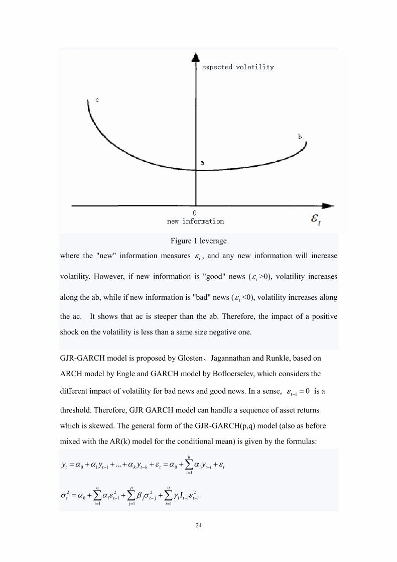
as leverage. The view for leverage is shown as Figure 1:

24

Figure 1 leverage

where the "new" information measures t , and any new information will increase

volatility. However, if new information is "good" news ( t >0), volatility increases

along the ab, while if new information is "bad" news ( t <0), volatility increases along

the ac. It shows that ac is steeper than the ab. Therefore, the impact of a positive

shock on the volatility is less than a same size negative one.

GJR-GARCH model is proposed by Glosten、Jagannathan and Runkle, based on

ARCH model by Engle and GARCH model by Bofloerselev, which considers the

different impact of volatility for bad news and good news. In a sense, 1 0t is a

threshold. Therefore, GJR GARCH model can handle a sequence of asset returns

which is skewed. The general form of the GJR-GARCH(p,q) model (also as before

mixed with the AR(k) model for the conditional mean) is given by the formulas:

0 1 1 01

...k

t t k t k t i t i ti

y y y y

2 2 2 20

1 1 1

q p q

t i t i j t j i t i t ii j i

I

25

t t tz

where the random variables tz are independent identically distributed with mean 0

and standard deviation 1. Here

1, 0

0, 0t

tt

I

.

The other restrictions that are added mainly to guarantee stationarity are as follows:

max 0,i i

0i

1 1 1

11

2

q p q

i i ii j i

.

4.4 QMLE (Quasi Maximum Likelihood Estimation)

Now, we introduce the QMLE (Quasi Maximum Likelihood Estimation), which is the

method to estimate parameters of GARCH model. We would like to present

GJR-GARCH(1,1) model for example. In comparison with the above description, we

change the notation -from now on 0 , 0 , 2t th .

The model is

t tr ,

2 21 1 1 1t t t t th h I

where , , , , is the set of parameters.

We have the likelihood function

1

( )n

tt

L l

,

where 2

22

log( ( ))( )t

t tt

rl h

h

.

If we define

26

ˆ arg max ( )L

,

then ̂ will be the QMLE, and ˆ ˆˆ ˆ ˆˆ, , , , will be the estimated parameters.

5 ES under FHS with GJR-GARCH Model

We follow an asymmetric GARCH specification named GJR-GARCH model, based

on Glosten, Jagannathan and Runkle (1993), with an empirical innovation density, to

fit the equity index return. Then estimate the ES under FHS.

(1) Observed data

Considering a securities market, we have

1ln lnt t tr p p

where tp is the equity index, tr is the daily log return of equity index. So the

observed data (returns) are 1 2, ,..., sr r r for 1, 2,...,t s , where t represents “days”.

(2) Set up GJR-GARCH(1,1) model

Here we fit a GJR-GARCH (1, 1) time series model in modeling the equity index

return to our data set. Under the historical measure P, the model is:

t tr (1)

2 21 1 1 1t t t t th h I (2)

The random variables t (noises) are assumed to:

1 0t tE F (3)

21t t t tVar F h (4)

where tF symbolizes information available at time t.

27

Such that the standard residuals are:

tt

t

zh

(5)

where ~ (0,1)tz f and tz are i.i.d (independent identically distributed).

Here is the constant expected return of the log return, , , , is the

parameters of the volatility equation (2). 1 1tI when 1 0t and 1 0tI

otherwise.

It is clear that for 0 , past negative return shocks ( 1 0t ) will have more

impact on future volatility. To ensure any solution th of equation (2) is positive, it is

assumed that , , , 0 .

(3) Calibration of the model

We use QMLE (Quasi Maximum Likelihood Estimation) method to find coefficients

of the model based on the empirical observed data 1 2, ,..., sr r r . After estimating the

parameters of the model, we can get the estimated value:

ˆ ˆˆ ˆ ˆˆ , , , , .

So under P measure we get the calibrated model for 1,2,...,t s :

ˆˆ ˆt tr (6)

2 21 1 1 1

ˆ ˆˆˆ ˆ ˆ ˆ ˆt t t t th h I (7)

ˆˆ

ˆt

t

t

zh

(8)

(4) Calculation of historical standard residuals

Using the calibrated model and the empirical observed data 1 2ˆ ˆ ˆ, ,..., sr r r (the same as

28

1 2, ,..., sr r r ) for 1,2,...,t s , we calculate and get historical standard residuals

1 2ˆ ˆ ˆ, ,..., sz z z .

The algorithm contains the following steps.

Step 1

Assumed initial values:

0ˆ 0 , 0

ˆˆˆˆ ˆ1 / 2

h

Initial standard residual:

00

0

ˆˆ 0

ˆz

h

Step 2

Set up for 1,2,...,t s :

(a)According to equation (6), we can get t̂ . That is (6) ˆˆ equationt tr .

(b)Put 1t̂ and 1ˆth in equation (7) and receive ˆ

th . That is (7)1 1

ˆ ˆˆ , equationt t th h .

(c) By equation (8) and get ˆtz . That is ˆ

ˆˆt

t

t

zh

.

(d) Repeat the (a) (b) (c) steps above for 1, 2,...,t s and get the result 1 2ˆ ˆ ˆ, ,..., sz z z .

(5) Filtered Historical Simulation

Suppose that at time s, we want to simulate the returns for the next T days. We select

* * *1 2, ,...,s s s Tz z z at random with replacement from the set 1 2ˆ ˆ ˆ, ,..., sz z z . The data

for time s is known. Using the model to calculate future returns in T days for the dates

1, 2,...,t s s s T is as below:

* * * 2 * 21 1 1 1

ˆˆ ˆ ˆt t t t th h I (9)

* * *t t tz h (10)

29

* *ˆt tr (11)

The algorithm contains the following steps.

Step 1

Select a set

* * *1 2, ,...,s s s Tz z z

which has T elements, and is chosen randomly with replacement from 1 2ˆ ˆ ˆ, ,..., sz z z .

Step 2 Assumed initial value:

* ˆs sh h , * ˆ

s s

Step 3

Set up for 1, 2,...,t s s s T :

(a) Put *1th and *

1t in equation (9) and get *th . That is (9)* * *

1 1, equationt t th h .

(b) Through equation (10) we receive *t . That is * * *

t t tz h .

(c) Put *t in equation (11), we can get *

tr . That is (11)* *equationt tr .

Step 4

This procedure is repeated N times which is as the number of simulations. Then we

can obtain N simulated returns:

* * *1 , 2 ,...,t t tr r r N , for 1, 2,...,t s s s T .

These predicted returns allow us to calculate predicted simulated values of the index

in T days:

* *

1

exp( )s T

s T i si s

p j r j p

, 1, 2,...,j N .

The values

*j s T sX p j p , 1, 2,...,j N

30

will be used in the calculation of the expected shortfall.

We can denote these predictions by

1 2, ,..., NX X X .

(6) ES (Estimating expected shortfall)

Let 1 2, ,..., NX X X be N independent samples drawn from the same probability

distribution. The same sequence reordered increasingly is denoted as

* * *1 2, ,..., NX X X .

Then an estimate of ES at level is given by

*

1

1 N

ii

ES XN

where N denotes the integer part of N that is rather big.

6 Empirical Analysis

We select the Shanghai Composite Index (SHCI), which is so important for Chinese

securities market. The data samples are from Wind database. We do two empirical

analysis under 2000.1.1~2007.5.31, and 2008.1.1~2010.5.31（under financial crisis）.

We propose that 20000N , and 0.05 .

In a securities market, we have tr , which is the daily log return of equity index,

represented as

1ln lnt t tr p p ,

where tp is the equity index.

For 2000.1.1~2007.5.31:

1. The basic characteristics of statistical data:

31

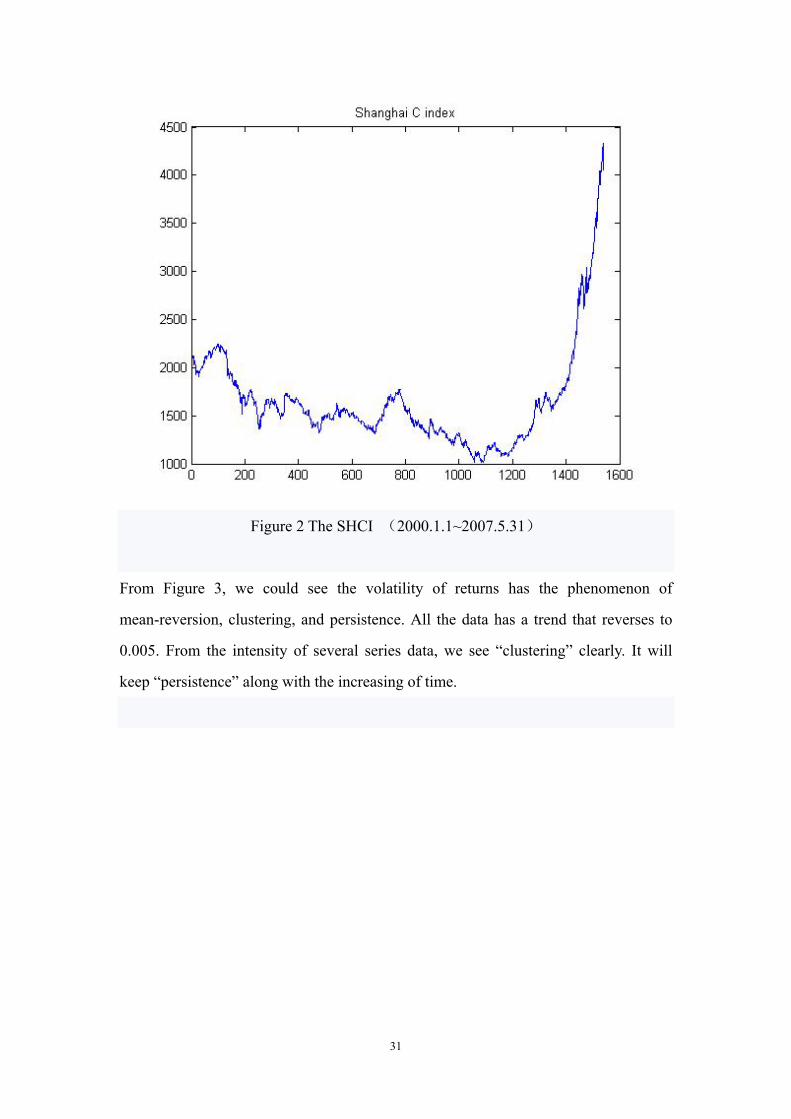
Figure 2 The SHCI （2000.1.1~2007.5.31）

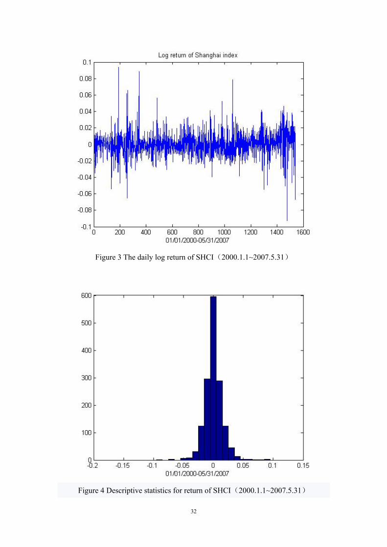
From Figure 3, we could see the volatility of returns has the phenomenon of

mean-reversion, clustering, and persistence. All the data has a trend that reverses to

0.005. From the intensity of several series data, we see “clustering” clearly. It will

keep “persistence” along with the increasing of time.

32

Figure 3 The daily log return of SHCI（2000.1.1~2007.5.31）

Figure 4 Descriptive statistics for return of SHCI（2000.1.1~2007.5.31）

33

The characters of statistics are described as Table 1:

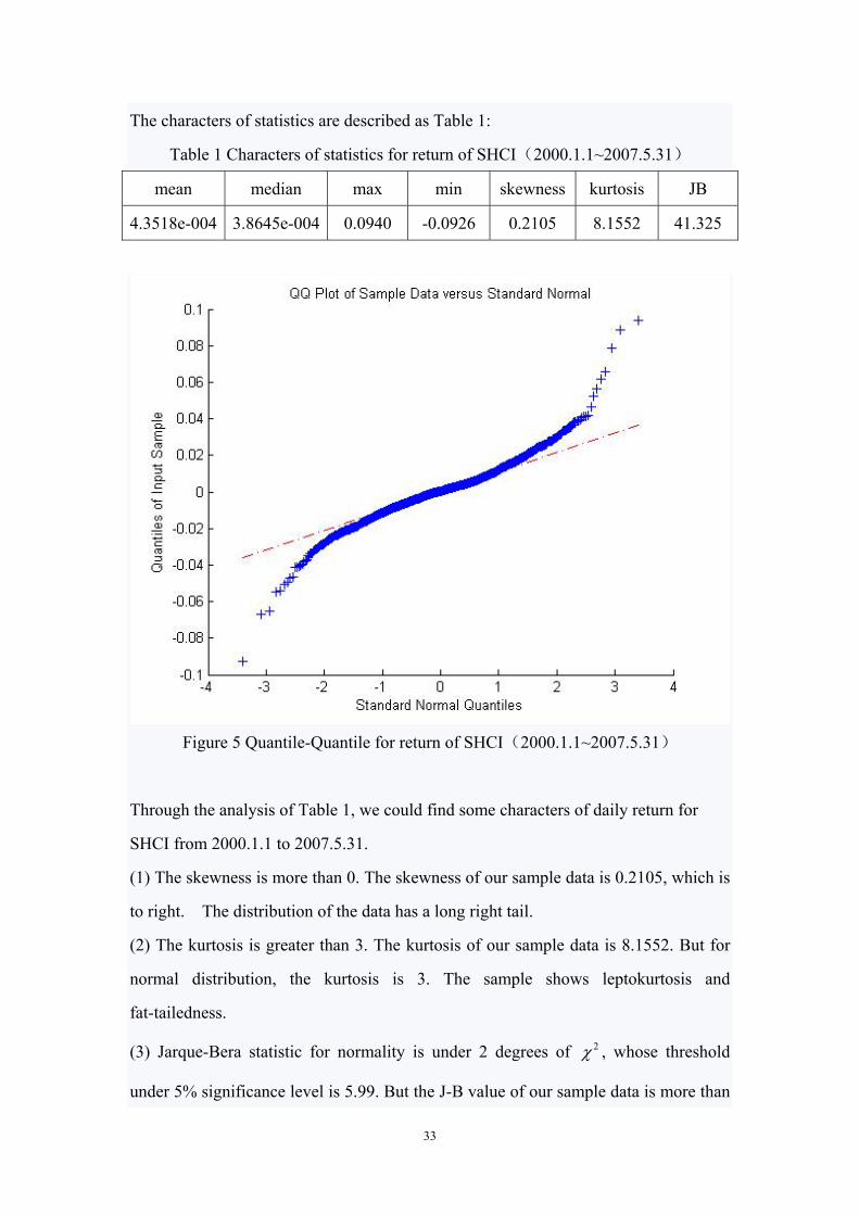
Table 1 Characters of statistics for return of SHCI（2000.1.1~2007.5.31）

mean median max min skewness kurtosis JB

4.3518e-004 3.8645e-004 0.0940 -0.0926 0.2105 8.1552 41.325

Figure 5 Quantile-Quantile for return of SHCI（2000.1.1~2007.5.31）

Through the analysis of Table 1, we could find some characters of daily return for

SHCI from 2000.1.1 to 2007.5.31.

(1) The skewness is more than 0. The skewness of our sample data is 0.2105, which is

to right. The distribution of the data has a long right tail.

(2) The kurtosis is greater than 3. The kurtosis of our sample data is 8.1552. But for

normal distribution, the kurtosis is 3. The sample shows leptokurtosis and

fat-tailedness.

(3) Jarque-Bera statistic for normality is under 2 degrees of 2 , whose threshold

under 5% significance level is 5.99. But the J-B value of our sample data is more than

34

5.99, which rejects the null hypothesis of normal distribution. It means that the series

tr is not normal distribution, which could also be seen from the figure 5 of Q-Q.

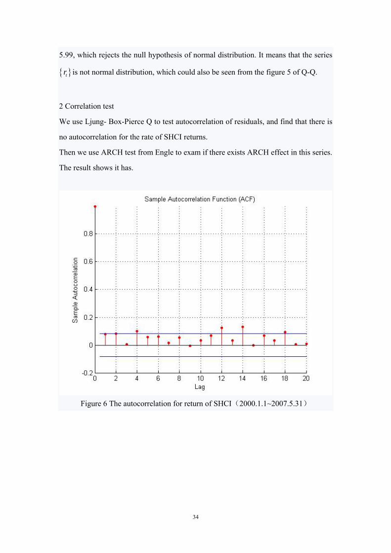
2 Correlation test

We use Ljung- Box-Pierce Q to test autocorrelation of residuals, and find that there is

no autocorrelation for the rate of SHCI returns.

Then we use ARCH test from Engle to exam if there exists ARCH effect in this series.

The result shows it has.

Figure 6 The autocorrelation for return of SHCI（2000.1.1~2007.5.31）

35

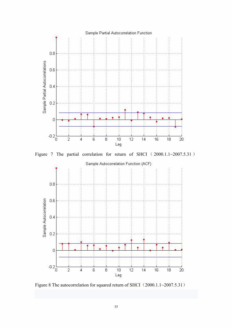
Figure 7 The partial correlation for return of SHCI （ 2000.1.1~2007.5.31 ）

Figure 8 The autocorrelation for squared return of SHCI（2000.1.1~2007.5.31）

36

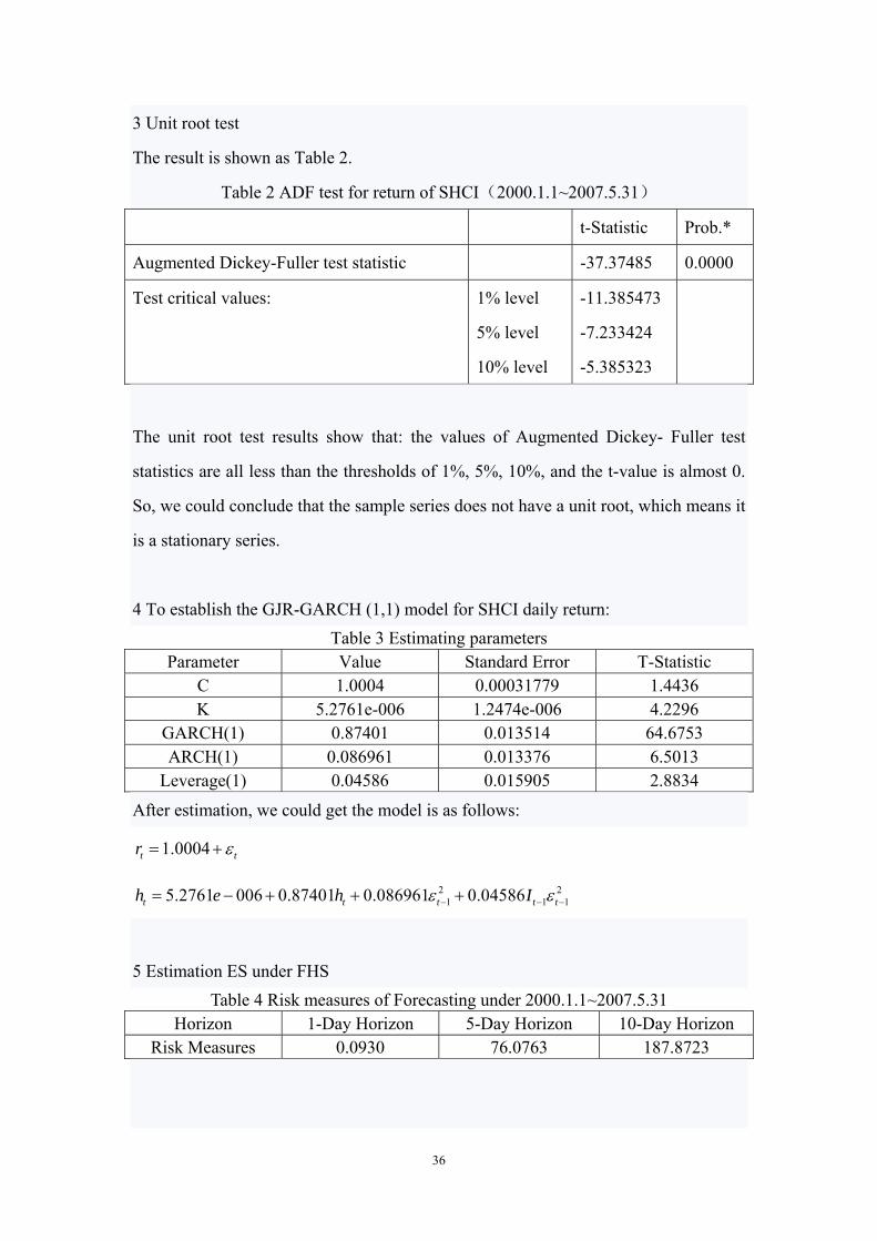
3 Unit root test

The result is shown as Table 2.

Table 2 ADF test for return of SHCI（2000.1.1~2007.5.31）

t-Statistic Prob.*

Augmented Dickey-Fuller test statistic -37.37485 0.0000

Test critical values: 1% level

5% level

10% level

-11.385473

-7.233424

-5.385323

The unit root test results show that: the values of Augmented Dickey- Fuller test

statistics are all less than the thresholds of 1%, 5%, 10%, and the t-value is almost 0.

So, we could conclude that the sample series does not have a unit root, which means it

is a stationary series.

4 To establish the GJR-GARCH (1,1) model for SHCI daily return:

Table 3 Estimating parameters Parameter Value Standard Error T-Statistic

C 1.0004 0.00031779 1.4436

K 5.2761e-006 1.2474e-006 4.2296

GARCH(1) 0.87401 0.013514 64.6753

ARCH(1) 0.086961 0.013376 6.5013

Leverage(1) 0.04586 0.015905 2.8834

After estimation, we could get the model is as follows:

1.0004t tr

2 21 1 15.2761 006 0.87401 0.086961 0.04586t t t t th e h I

5 Estimation ES under FHS

Table 4 Risk measures of Forecasting under 2000.1.1~2007.5.31 Horizon 1-Day Horizon 5-Day Horizon 10-Day Horizon

Risk Measures 0.0930 76.0763 187.8723

37

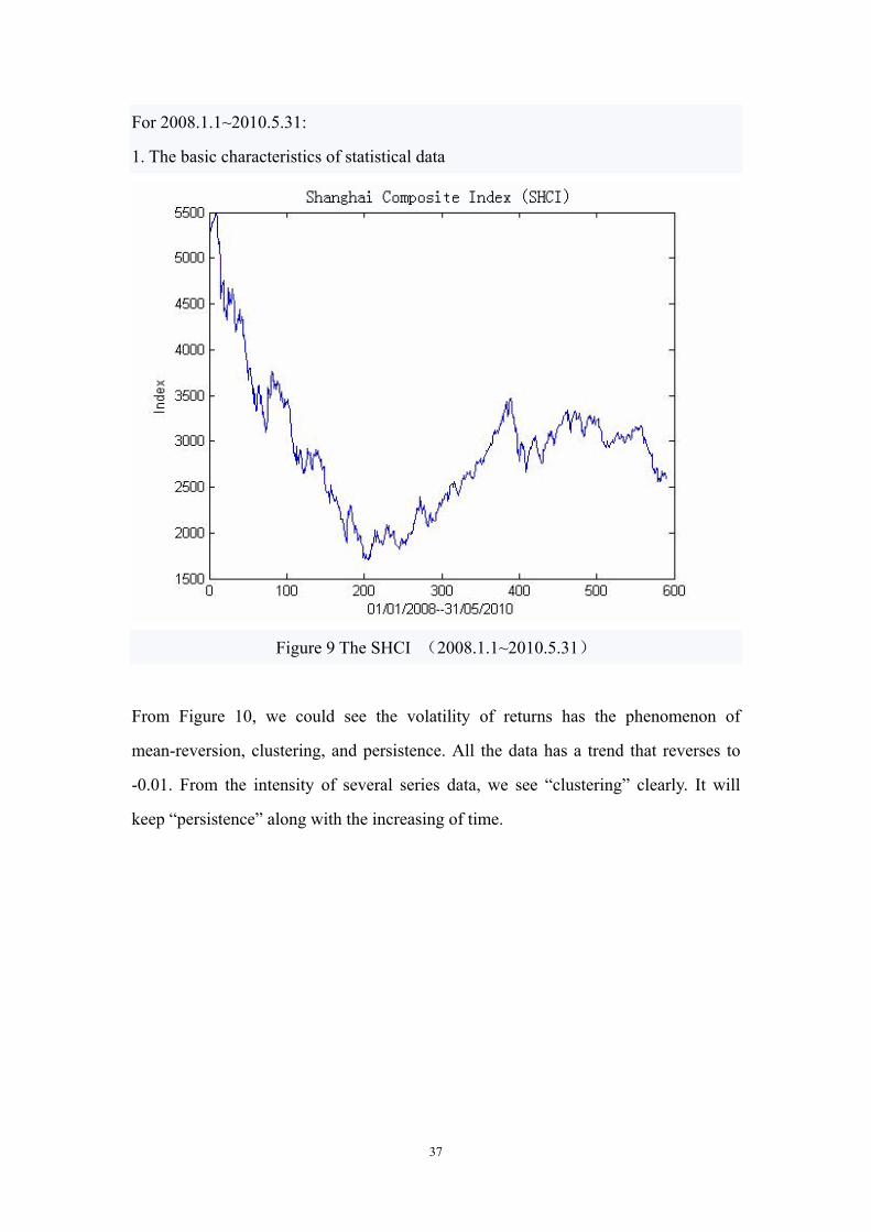
For 2008.1.1~2010.5.31:

1. The basic characteristics of statistical data

Figure 9 The SHCI （2008.1.1~2010.5.31）

From Figure 10, we could see the volatility of returns has the phenomenon of

mean-reversion, clustering, and persistence. All the data has a trend that reverses to

-0.01. From the intensity of several series data, we see “clustering” clearly. It will

keep “persistence” along with the increasing of time.

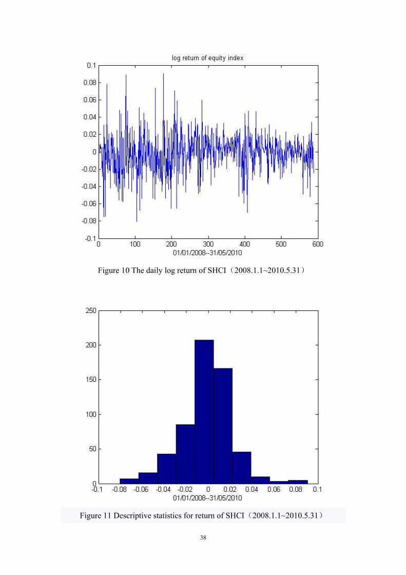
38

Figure 10 The daily log return of SHCI（2008.1.1~2010.5.31）

Figure 11 Descriptive statistics for return of SHCI（2008.1.1~2010.5.31）

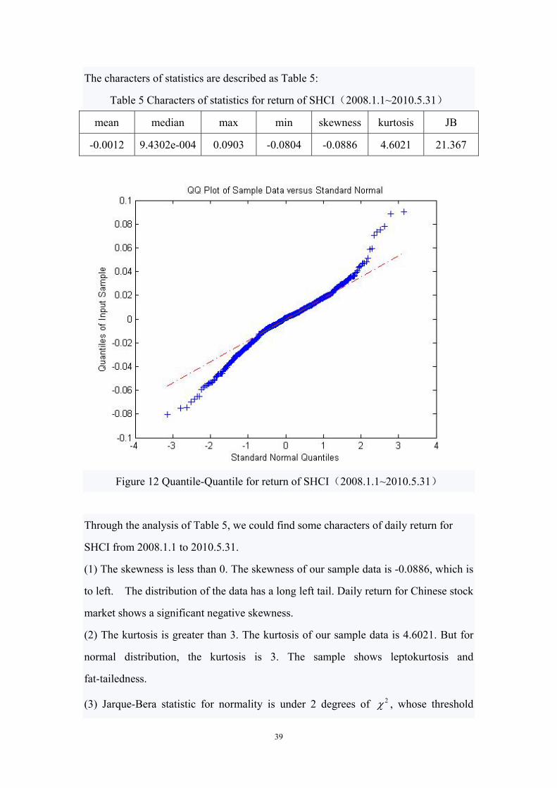
39

The characters of statistics are described as Table 5:

Table 5 Characters of statistics for return of SHCI（2008.1.1~2010.5.31）

mean median max min skewness kurtosis JB

-0.0012 9.4302e-004 0.0903 -0.0804 -0.0886 4.6021 21.367

Figure 12 Quantile-Quantile for return of SHCI（2008.1.1~2010.5.31）

Through the analysis of Table 5, we could find some characters of daily return for

SHCI from 2008.1.1 to 2010.5.31.

(1) The skewness is less than 0. The skewness of our sample data is -0.0886, which is

to left. The distribution of the data has a long left tail. Daily return for Chinese stock

market shows a significant negative skewness.

(2) The kurtosis is greater than 3. The kurtosis of our sample data is 4.6021. But for

normal distribution, the kurtosis is 3. The sample shows leptokurtosis and

fat-tailedness.

(3) Jarque-Bera statistic for normality is under 2 degrees of 2 , whose threshold

40

under 5% significance level is 5.99. But the J-B value of our sample data is more than

5.99, which rejects the null hypothesis of normal distribution. It means that the series

tr is not normal distribution, which could also be seen from figure 12 of Q-Q.

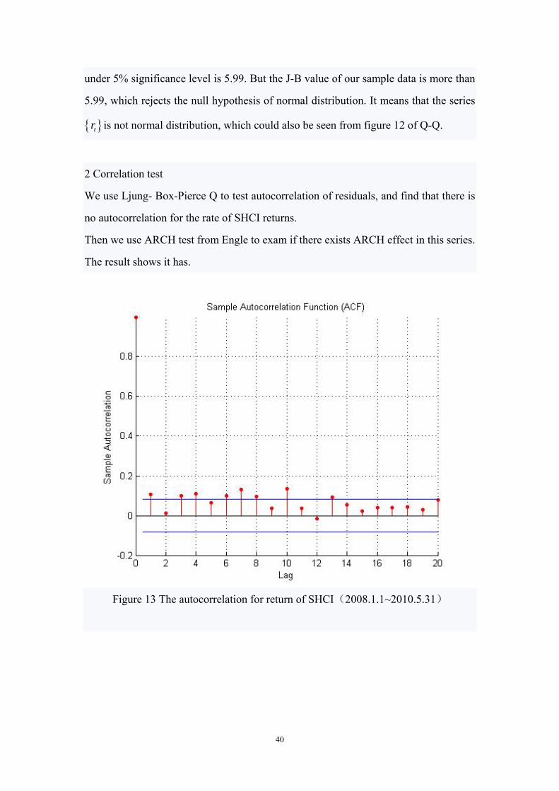
2 Correlation test

We use Ljung- Box-Pierce Q to test autocorrelation of residuals, and find that there is

no autocorrelation for the rate of SHCI returns.

Then we use ARCH test from Engle to exam if there exists ARCH effect in this series.

The result shows it has.

Figure 13 The autocorrelation for return of SHCI（2008.1.1~2010.5.31）

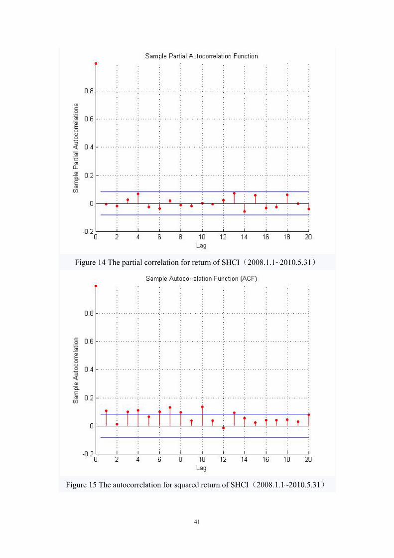
41

Figure 14 The partial correlation for return of SHCI（2008.1.1~2010.5.31）

Figure 15 The autocorrelation for squared return of SHCI（2008.1.1~2010.5.31）

42

3 Unit root test

The time series using in GARCH model should be stationary. So we use the

Augmented Dickey-Ful1er test (ADF) to exam if the sample has unit root, which can

show if the sample series is stationary. We chose to use Schwazrh Information

Criterion (SIC), and let the computer automatically select the lag, setting the

maximum lag order be 10. The result is shown as Table 6.

Table 6 ADF test for return of SHCI（2008.1.1~2010.5.31）

t-Statistic Prob.*

Augmented Dickey-Fuller test statistic -29.92783 0.0000

Test critical values: 1% level

5% level

10% level

-6.374853

-4.357743

-3.384722

The unit root test results show that: the values of Augmented Dickey- Fuller test

statistics are all less than the thresholds of 1%, 5%, 10%, and the t-value is almost 0.

So, we could conclude that the sample series does not have a unit root, which means it

is a stationary series.

4 To establish the GJR-GARCH (1,1) model for SHCI daily return:

Table 7 Estimating parameters

Parameter Value Standard Error T-Statistic C 0.9988 0.00087391 0.5832 K 1.0154e-005 3.2139e-006 3.1594

GARCH(1) 0.92151 0.017158 53.7064 ARCH(1) 0.01656 0.015008 1.1034

Leverage(1) 0.077807 0.022786 3.4148

After estimation, we could get the model is as follows:

0.9988t tr

2 21 1 11.0154 005 0.92151 0.01656 0.077807t t t t th e h I

5 Estimation ES under FHS

43

Table 8 ES of Forecasting under 2008.1.1~2010.5.31 Horizon 1-Day Horizon 5-Day Horizon 10-Day Horizon

ES 0.1862 259.3408 528.3150

44

References

[1] Artzner P, Delbaen F, Eber J M, et al. Thinking coherently [J]. Risk, 1997, 10:

68-71

[2] Acerbi C, Tasche D. On the coherence of expected shortfall, Banking and Finance,

2002, 26: 1487-1503

[3] Bollerslev Tim. Generalized autoregressive conditional heteroseedasticity，Journal

of econometrics，1986, 31: 307一327

[4] Barone-Adesi, G., Giannopoulos, K., Vosper, L. (2000), Filtered Historical

Simulation; Backtest Analysis, Working Paper, University of Westminster

[5] Barone-Adesi G, Giannopoulos K, Vosper L. Backtesting derivative portfolios

with filtered historical simulation, European Financial Management, 2002, 8: 31-58

[6] E. Ghysels, A. Harvey and E. Renault. Stochastic volatility, in G. Maddala and C.

Rao (eds), Statistical Methods in Finance, 1996, Vol. 14 of Handbook of Statistics

[7] Engle R F. Autoregressive conditional heteroscedastieity with estimate of the

variance of united Kingdom inflation，econometrica，1982,31: 987一1005

[8] Ghashang Piroozfar (2009), Forecasting Value at Risk with Historical and

Filtered Historical Simulation Methods, U.U.D.M. Project Report 2009:15

[9] Giannopoulos K, Tunaru R. Coherent risk measures under filtered historical

simulation. Journal of Banking and Finance, 2005, 29: 979-996

[10] http://baike.baidu.com/view/131677.htm#8

[11] 雷乐(2008), 基于GJR-GARCH、FHS、Copula和极值理论的中国证券市场

VaR模型研究，UDC 17, page 2

[12] 滕帆，金融风险度量：一个文献综述，浙江大学宁波理工学院，浙江宁波

315100

Appendix: Matlab source code

One day code (2000.1.1~2007.5.31) Clear

45

Load shanghai.mat u=1.0004;

w=5.2761e-006; beta=0.87401; alpha=0.086961; gamma=0.04586; h=[1539,1]; sunn=[]; h0=w/(1-alpha-beta); e0=0; z0=0; zhzuan=0; z=[1539,1]; e=[1539,1]; rtest=[20000,1]; h(1)=w+beta*h0; z(1)=e(1)/sqrt(h(1)); for i=1:1539 e(i)=yy1(i)-u; end for i=2:1539 if e(i-1)<0 h(i)=w+beta*h(i-1)+alpha*e(i-1)^2+gamma*e(i-1)^2; else h(i)=w+beta*h(i-1)+alpha*e(i-1)^2; end end for i=2:1539 z(i)=e(i)/sqrt(h(i)); end for j=1:20000 htest=w+beta*h(1539)+alpha*e(1539)^2+gamma*e(1539)^2; index=1+round(rand(1)*1538); etest=z(index)*sqrt(htest); rtest(j)=exp(etest+u)*4109.65-4109.65; end rnew=sort(rtest); for i=1:1000 sum=0; sum=sum+rnew(i); end aver=-sum/1000 Five day code

46

Clear Load shanghai.mat u=1.0004;

w=5.2761e-006; beta=0.87401; alpha=0.086961; gamma=0.04586; h=[1539,1]; sunn=[]; h0=w/(1-alpha-beta); e0=0; z0=0; zhzuan=0; z=[1539,1]; ztest=[5,1]; e=[1539,1]; etest=[1539,1]; rtest=[5,1]; h(1)=w+beta*h0; z(1)=e(1)/sqrt(h(1)); hhtest=[5,1]; for i=1:1539 e(i)=yy1(i)-u; end for i=2:1539 if e(i-1)<0 h(i)=w+beta*h(i-1)+alpha*e(i-1)^2+gamma*e(i-1)^2; else h(i)=w+beta*h(i-1)+alpha*e(i-1)^2; end end for i=2:1539 z(i)=e(i)/sqrt(h(i)); end for j=1:20000 for i=1:5 index=1+round(rand(1)*1538); ztest(i)=z(index); end hhtest(1)=w+beta*h(1539)+alpha*e(1539)^2+gamma*e(1539)^2; etest(1)=ztest(1)*sqrt(hhtest(1)); for n=2:5 if etest(n-1)<0

47

hhtest(n)=w+beta*hhtest(n-1)+alpha*etest(n-1)^2+gamma*etest(n-1)^2; %index=1+round(rand(1)*587); else hhtest(n)=w+beta*hhtest(n-1)+alpha*etest(n-1)^2; end etest(n)=ztest(n)*sqrt(hhtest(n)); end for nn=1:5 rtest(nn)=etest(nn)+u; end sunn=0; for i=1:5 sunn=sunn+rtest(i); end tol(j)=exp(sunn)*4109.65-4109.65; end %for j=1:42 %rtest(j)=etest(j)+u; %end rnew=sort(tol); sum=0; for i=1:1000 sum=sum+rnew(i); end aver=-sum/1000