PORTFOLIO SELECTION UNDER CONTINUOUS SHORTFALL CONSTRAINTS

Davide Maspero

IEMIF – Istituto di Economia degli Intermediari Finanziari

Università Commerciale Luigi Bocconi

Viale Isonzo 25

20136 Milano

davide.maspero@unibocconi.it

tel +39 02 58365862

fax +39 02 58365920

1

ABSTRACT

Most of the financial planning theory is based on the evaluation of terminal wealth within a single-period model. Even when the impact of different time horizons is considered, this is done by

comparing the probabilistic terminal outcomes of the investments.This perspective fails to capture the importance of controlling the maximum probabilistic loss during the investment period.

Investments yielding similar terminal probabilistic outcomes can have dramatically different in-period potential loss profiles. This paper develops a lognormal model in which probabilistic losses

are monitored within the whole investment period. Consistently, a continuous shortfall line is developed.

2

1. INTRODUCTION

The investment process is generally characterized by three main steps:

- the identification of efficient portfolios defined in terms of broad asset classes, traditionally represented by benchmark indices;

- the selection of one of these efficient portfolios on the basis of the investor’s preferences, needs and financial goals.

- the construction of the actual investment portfolio through instruments (mutual funds or individual securities) that match the original target asset allocation, while allowing for the desired amount of active risk and expected active return against the benchmark

Each step is equally critical and failure to adequately handle it can substantially deteriorate the outcome of the investment process.

Efficient frontier construction is affected by estimation risk, as all the parameters necessary to derive ex-ante frontiers have to be estimated. Errors in the estimation of the optimization input parameters are amplified by the optimization procedure itself, so that ex-post performance of supposedly efficient portfolios can be dramatically disappointing. The estimation of expected return is especially critical, as the weights of asset classes in efficient portfolios can be extremely sensitive to slight changes in the vector of expected returns.

Poor assessment of investors’ preferences and risk tolerance can lead to substantial dissatisfaction once the misalignment between investors’ needs and portfolio characteristics becomes evident. A correct evaluation of an investor’s risk attitude is a task of extreme complexity, as it requires not only a diligent representation of the investor’s financial present and prospective conditions, but also a deep understanding of his/her emotional tolerance of financial risk. This aspect hardly fits into any of the currently accepted investment selection models.

Finally, poor choice of individual investment products can destroy the value created at the asset allocation levels. There are different reasons for this. First of all, the selection of individual investment products is based on incomplete information. Second, individual investment products can fail to adequately represent the asset classes used in the optimization procedure; this failure can derive from explicit inconsistency of investment policy with the stated objectives of the fund or from manager changes or style drifts. Finally, the quest for active return by the fund manager can yield results that are inconsistent with expectations. Active management of asset classes characterized by high levels of efficiency very often turns out to be detrimental once management costs are considered.

This paper deals with the problem outlined in point b) before. Failure to adequately incorporate the assessment of investor’s needs and preferences in investment decisions can have disastrous consequences, no matter how well stages a) and c) are performed.

In the first part of the paper a portfolio selection model is outlined. The model is developed in a lognormal continuous-time setting, which allows both analytical simplicity and a natural consideration of the effect of time diversification. This model also allows for the definition of

3

financial goals in terms of shortfall or portfolio Value at Risk. The model shows that, even when a financial goal is clearly defined by the customer, three different efficient portfolios can be considered “best” at the same time. Though occasionally two of the three or all the three portfolios will coincide, in most practical situations they will differ substantially in terms of composition and risk/return characteristics. This ambiguity, which is implicit in the financial planning decision, stems from the fact that the financial objective is defined by a combination of desired wealth, time horizon and confidence level. Depending on which of these elements has a priority in the investor’s preferences, different portfolios will be chosen.

In order to further improve the assessment of investor’s preferences an additional criterion is then introduced in the second part of the paper. Given the long-term nature of many investment goals, investors heavily (though often unconsciously) rely on time diversification to achieve their shortfall objectives at maturity, indicating a minimum return they want achieved – or a maximum loss they don’t want to be exceeded - with given probability. However at times investors will realize – often with harsh surprise – that this maximum probabilistic loss can be exceeded substantially during the life of the investment. This event, though consistent with the notion of time diversification, can lead investors to precipitous - and often untimely - changes in their portfolio composition. It may then be important that investors be informed on the maximum probabilistic loss they might experience during the whole planned investment period, and not just at maturity. We therefore propose a Continuous Time Shortfall constraint, identifying portfolios that satisfy a maximum loss probabilistic bound throughout the life of the investment. The introduction of this additional constraint can further reduce the set of optimal portfolios, thus enabling the financial planner to make a more informed decision.

4

2. A GENERAL CONTINUOUS - TIME LOGNORMAL MODEL FOR FINANCIAL PLANNING DECISIONS

2.1 Introduction to the model

Most of the portfolio selection literature is developed in a single-period framework. The single-period framework, although simple and effective in outlining the major financial investment concepts, cannot handle investment decisions when different time horizons are to be considered. Furthermore, investors are sometimes able to identify their investment horizon as “long”, but unable to translate this concept in a precise number of years, so that the possibility to change the investment horizon within the model can be useful.

These considerations led us to the choice of a lognormal continuous-time model, which allows time to be included as a fundamental variable in the financial planning problem.

One major problem with the lognormal hypothesis is that the sum of lognormally distributed returns (or return relatives) is not itself lognormally distributed. Therefore the assumption of lognormality at the individual asset return level is inconsistent with the assumption of lognormality at the portfolio level. Usually this problem is countered by the observation that lognormality at the portfolio level, while not being formally correct, is a good approximation of the distribution of the sum of lognormal asset returns. We will however get away with this objection by assuming that portfolios (and wealth in general) be lognormally distributed, without further assumptions on the distribution of individual assets.

The lognormal model we will be using is derived from the hypothesis of Geometric Brownian Motion as the stochastic process driving the evolution of wealth over time. This is consistent, among the others, with the original Black & Scholes assumption and, in a more pertinent framework, with the Ibbotson-Sinquefield original work of 1976. Though Ibbotson and Sinquefield’s model was empirical in nature, it was later shown1 to be equivalent to the assumption of Geometric Brownian Motion. This aspect was further clarified by Kaplan (2000).

Although we understand that leptokurtosis of return distribution is a concern, we think that only the normal/lognormal model can allow the time dimension to be treated effectively without excessive analytical complexity. Furthermore, departure from the normal/lognormal model would have

1 Lewis, Kassouf, Brehm, Johnston (1980).

5

required a specification of the alternative assumptions concerning the distribution of asset returns, either in a nonparametric or parametric approach.

2.2 The model

We assume the market value W of a generic portfolio to follow Geometric Brownian Motion WdZWdtdW ση += (1)

where dtdZ ε= and )1,0(N≈ε .

Under this hypothesis

[ TTNWWT σµ ,ln

0

≈⎟⎟⎠

⎞⎜⎜⎝

⎛ ] (2)

where 2

2σηµ −= .

Quantiles of the distribution of portfolio market values at time T can be calculated as

( )TzTWW pp

T σµ +⋅= exp0 (3)

where is such that given a standardized normal Z pz

Prob ( ) pzZ p =<

A value of = 0 leads to the median of portfolio market value at time T being pz

( TWWT µexp050.0 ⋅= ) (4)

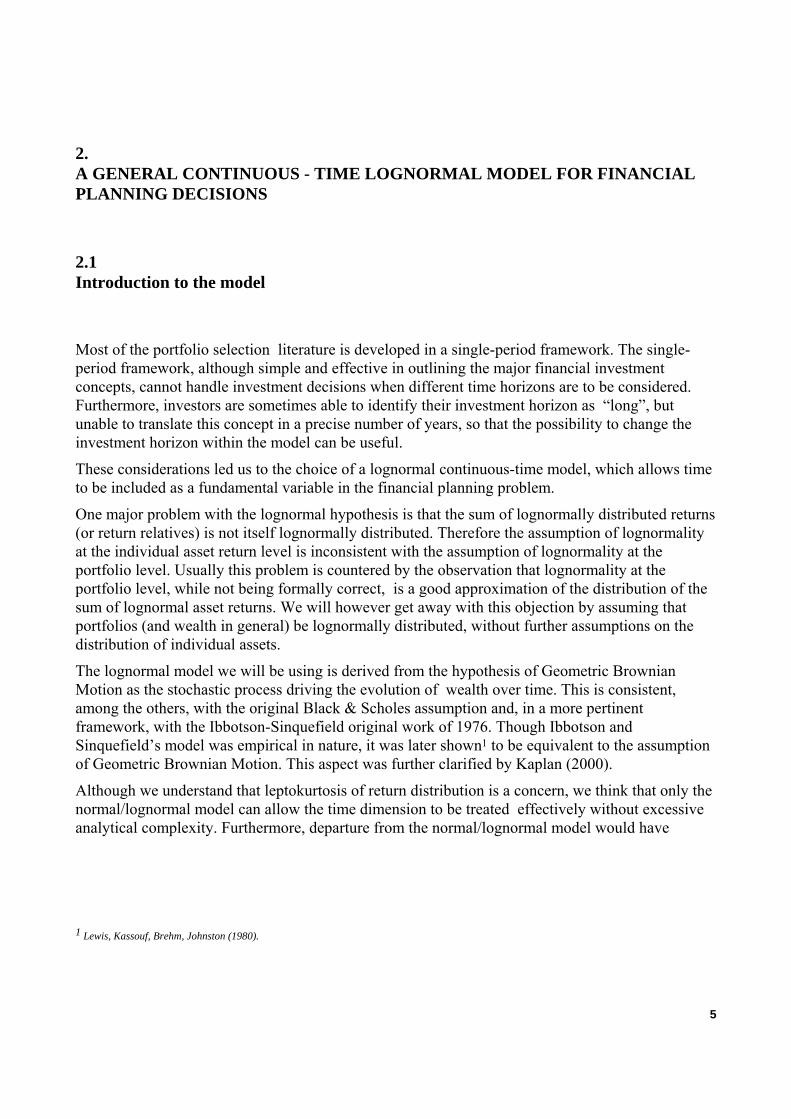
Figure 1a and 1b represent the probabilistic evolution of wealth over 10 years for a portfolio with µ= 10% and σ= 15%. The upper line represents the 90th percentile, the lower line the 10th percentile and the intermediate line the median wealth of equation (4)

6

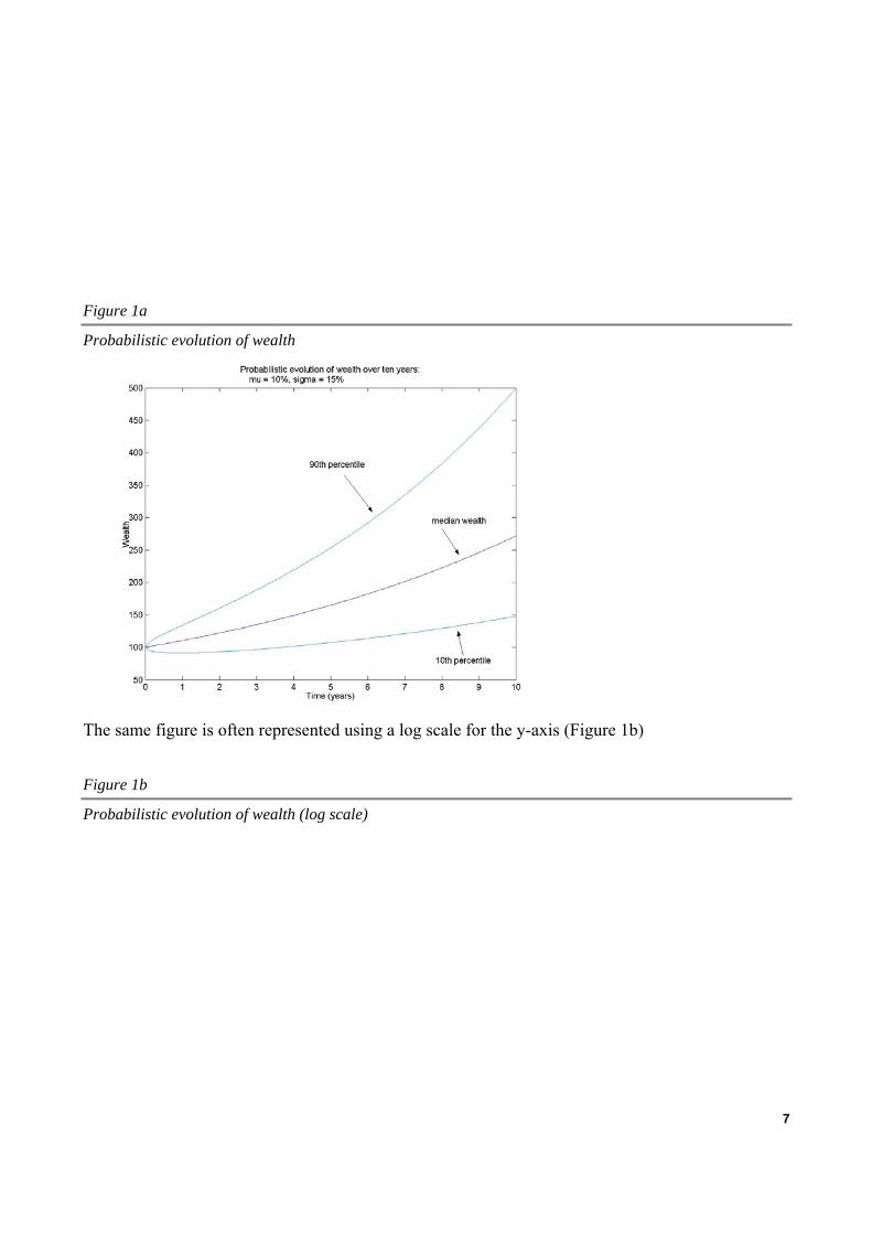
Figure 1a

Probabilistic evolution of wealth

The same figure is often represented using a log scale for the y-axis (Figure 1b)

Figure 1b

Probabilistic evolution of wealth (log scale)

7

2.3 The statement of financial planning goals

Equation (3) answers, under the assumptions of the model, an elementary financial planning question: given an initial capital and a time horizon T , which final wealth can be attained with confidence level p ?

0W TW

One nice feature of the model is that we can express analytically each of the four variables as a function of the other three. Each of these restatements answers a different financial planning question.

Restatement 1

TTWW

z Tp σ

µ−−=

)ln()ln( 0 (5)

Given an initial wealth , a time horizon T and a target wealth , what is the confidence level associated to this final wealth ? Since implies a probability p of achieving a final wealth lower than , then there is a (1-p) probability of achieving or greater.

0W TW

pz

TW TW

8

Restatement 2

( ) ( )[ ]µ

µσσ

2

lnln4 022 WWzz

T Tpp −++−= (6)

Given an initial wealth , how much time do we need to achieve a target wealth with a confidence level p associated to ?

0W TW

pz

Restatement 3

)exp(0 TzTWW pT σµ −−⋅= (7)

Given a target wealth , a confidence level p (associated to ) and a time horizon equal to T, what is the initial wealth needed to obtain this result ?

TW pz

Given the parameters µ and σ, equations (5) to (7) allow us to build a consistency table. A consistency table verifies whether the financial planning objective is feasible and identifies consistent quartets of the variables , , T and p. 0W TW

As an example, let’s assume that our portfolio will grow with an annualized expected return m equal to 7% and an annualized standard deviation s of 8%. These values are expressed with reference to discrete lognormal returns, and have to be translated into their continuous time equivalents. Following the conversion procedure outlined in Appendix this is consistent with µ = 6.49% and σ= 7.46%. Let’s then imagine that the financial planning goal be defined as follows: given an initial wealth of 100 and a time horizon of 5 years, the aim is to attain a final wealth of 115 with a 90% confidence level. This is equivalent to stating a 5-year shortfall risk of 10% of achieving less than 115.

Table 1

Consistency table for portfolio 1

0W TW T p

Target values 100 115 5 90% 107.46 115 5 90%

100 111.67 5 90% 100 115 6.60 90%

Consistent quartets

100 115 5 80.26%

The consistency table shows that this portfolio is not capable of satisfying the stated financial objectives. As an example, given the target wealth of 115 to be reached with a 90% confidence level and a time horizon of 5 years, the initial wealth should be of 107.46 and not 100. Similarly,

9

given an initial wealth of 100, the time horizon and the confidence level, the final wealth that can be reached with 90% confidence is just 111.67. Again, the time required to achieve a 90% confidence, given an initial wealth of 100 and a target final wealth of 130, would be 6.60 years. Finally, the stated financial objective can be reached only with 80.26% confidence in 5 years.

When, like in this example, a portfolio does not allow to meet the financial planning goals, either the portfolio is changed or the financial objectives must be restated. This implies choosing either a higher initial wealth or a lower final wealth or a longer time horizon or a lower confidence level (or, of course, a combination of these).

Now let’s imagine that a second more aggressive portfolio is available, with an annualized expected return m of 17% and an annualized standard deviation s of 20%. This translates to µ = 14.26% and σ= 16.97%. Given the same objectives as before, the new consistency table becomes the following.

10

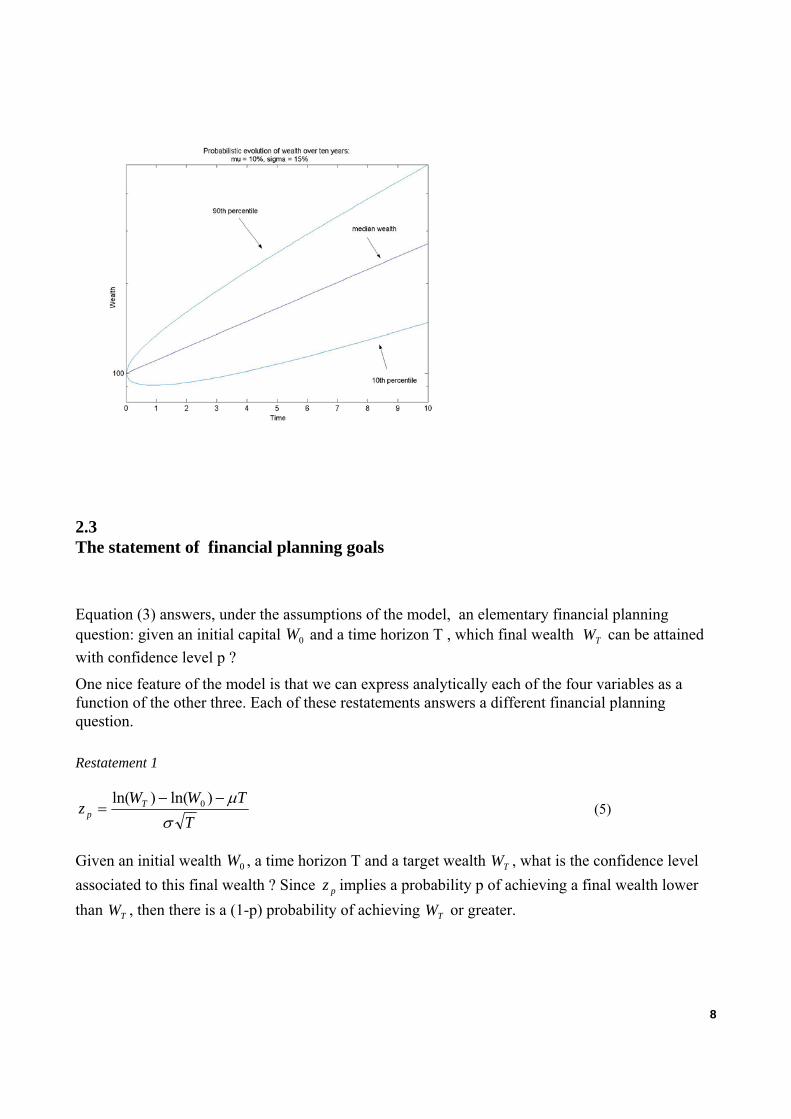
Table 2

Consistency table for portfolio 2

0W TW T p

Target values 100 115 5 90% 95.66 115 5 90% 100 125.44 5 90% 100 115 4.52 90%

Consistent quartets

100 115 5 91.90% The financial planning objectives are satisfied by this second portfolio. The values in the consistency tables should therefore be interpreted as the values which are sufficient to meet the stated financial objectives. As an example, given the 5-year horizon and a final wealth of 115 to be attained with 90% confidence level, an initial wealth of 95.66 would be sufficient. Similarly, investing 100 for 5 years would allow us to reach a final wealth of 125.44 with 90% confidence; the stated financial goals could be reached in 4.52 years instead than five; finally after 5 years we would have a 91.90% probability of achieving the investment goal.

In the following examples the consistency tables will be expressed synthetically, reporting just one line for each portfolio. Each element of the line is the dependent variable in equations (12) to (15) given that the other elements of the financial planning statement are the ones reported in the objective. As an example, the synthetic consistency table for the two portfolios and the financial objective stated before would look like table 3

Table 3

Synthetic consistency table

0W TW T p

Target values 100 115 5 90% Portfolio 1 107.46 111.67 6.60 80.26% Portfolio 2 95.66 125.44 4.52 91.90%

2.4 Portfolio choice and the ambiguity of the financial planning objective

In the previous examples the consistency tables were used to assess the effectiveness of a given portfolio in achieving stated financial goals.

11

When many alternative portfolios are available, portfolio selection implies choosing the “best” portfolio. We will show that, even when a financial objective is clearly stated, this notion of “best” portfolio is ambiguous most of the times. More than one portfolio can be considered best depending on the criterion which is used to assess how well the desired financial goals can be achieved with a given portfolio.

There are three elementary “best” portfolios:

The Wealth Portfolio is the portfolio that, given the initial wealth, the time horizon and the desired confidence level, achieves the highest final wealth. This is the same as the portfolio that, given the time horizon, the target final wealth and desired confidence level, requires the smallest initial wealth to achieve the objective.

The Time Portfolio is the portfolio that, given the initial wealth, the desired final wealth and the desired confidence level, achieves the goal in the shortest period of time.

The Confidence Portfolio is the portfolio that, given the initial wealth, the time horizon and the target final wealth, achieves the result with the highest confidence level.

Although all of these three elementary portfolios stem from the same financial objectives, they will often imply very different levels of expected return and volatility, and will therefore have substantially different compositions. In order to match available portfolios to investors’ financial goals it is therefore essential to identify which objective (wealth, time or confidence) is the investor’s priority.

An example of portfolio choice according to the three different criteria can best illustrate the point. Let’s assume an investor’s financial goal is the following: obtaining with a 90% confidence level 130 dollars out of an initial investment of 100 in 10 years. The investor has to choose among 21 available portfolios. The portfolios represent combinations of bonds and stocks having the following characteristics:

Expected return Standard deviation

Bonds 5% 5%

Stocks 15% 20%

Correlation coefficient 0.2

12

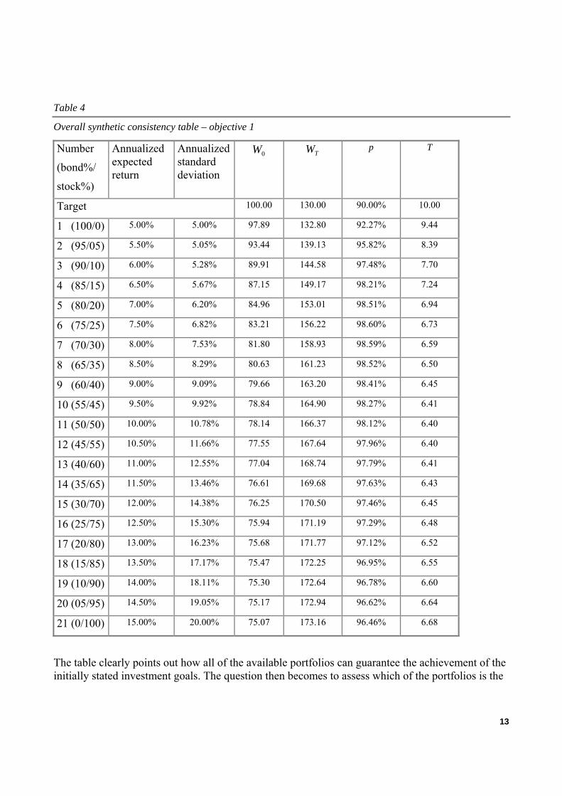
Table 4

Overall synthetic consistency table – objective 1

Number

(bond%/

stock%)

Annualized expected return

Annualized standard deviation

0W TW p T

Target 100.00 130.00 90.00% 10.00

1 (100/0) 5.00% 5.00% 97.89 132.80 92.27% 9.44

2 (95/05) 5.50% 5.05% 93.44 139.13 95.82% 8.39

3 (90/10) 6.00% 5.28% 89.91 144.58 97.48% 7.70

4 (85/15) 6.50% 5.67% 87.15 149.17 98.21% 7.24

5 (80/20) 7.00% 6.20% 84.96 153.01 98.51% 6.94

6 (75/25) 7.50% 6.82% 83.21 156.22 98.60% 6.73

7 (70/30) 8.00% 7.53% 81.80 158.93 98.59% 6.59

8 (65/35) 8.50% 8.29% 80.63 161.23 98.52% 6.50

9 (60/40) 9.00% 9.09% 79.66 163.20 98.41% 6.45

10 (55/45) 9.50% 9.92% 78.84 164.90 98.27% 6.41

11 (50/50) 10.00% 10.78% 78.14 166.37 98.12% 6.40

12 (45/55) 10.50% 11.66% 77.55 167.64 97.96% 6.40

13 (40/60) 11.00% 12.55% 77.04 168.74 97.79% 6.41

14 (35/65) 11.50% 13.46% 76.61 169.68 97.63% 6.43

15 (30/70) 12.00% 14.38% 76.25 170.50 97.46% 6.45

16 (25/75) 12.50% 15.30% 75.94 171.19 97.29% 6.48

17 (20/80) 13.00% 16.23% 75.68 171.77 97.12% 6.52

18 (15/85) 13.50% 17.17% 75.47 172.25 96.95% 6.55

19 (10/90) 14.00% 18.11% 75.30 172.64 96.78% 6.60

20 (05/95) 14.50% 19.05% 75.17 172.94 96.62% 6.64

21 (0/100) 15.00% 20.00% 75.07 173.16 96.46% 6.68

The table clearly points out how all of the available portfolios can guarantee the achievement of the initially stated investment goals. The question then becomes to assess which of the portfolios is the

13

“best” portfolio, given the investment goals. The highlighted portfolios give the answer to this question.

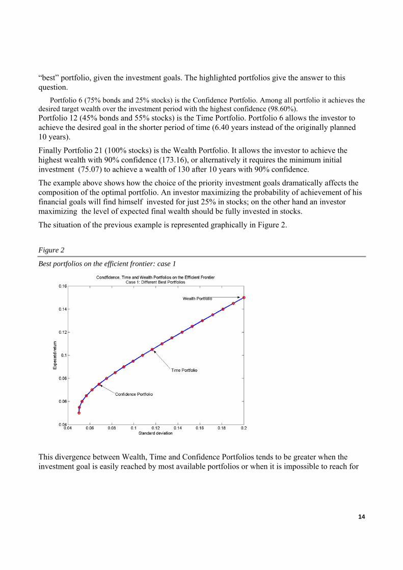
Portfolio 6 (75% bonds and 25% stocks) is the Confidence Portfolio. Among all portfolio it achieves the desired target wealth over the investment period with the highest confidence (98.60%). Portfolio 12 (45% bonds and 55% stocks) is the Time Portfolio. Portfolio 6 allows the investor to achieve the desired goal in the shorter period of time (6.40 years instead of the originally planned 10 years).

Finally Portfolio 21 (100% stocks) is the Wealth Portfolio. It allows the investor to achieve the highest wealth with 90% confidence (173.16), or alternatively it requires the minimum initial investment (75.07) to achieve a wealth of 130 after 10 years with 90% confidence.

The example above shows how the choice of the priority investment goals dramatically affects the composition of the optimal portfolio. An investor maximizing the probability of achievement of his financial goals will find himself invested for just 25% in stocks; on the other hand an investor maximizing the level of expected final wealth should be fully invested in stocks.

The situation of the previous example is represented graphically in Figure 2.

Figure 2

Best portfolios on the efficient frontier: case 1

This divergence between Wealth, Time and Confidence Portfolios tends to be greater when the investment goal is easily reached by most available portfolios or when it is impossible to reach for

14

all portfolios. On other occasions two or all the three “best” portfolios will coincide, like in the following example.

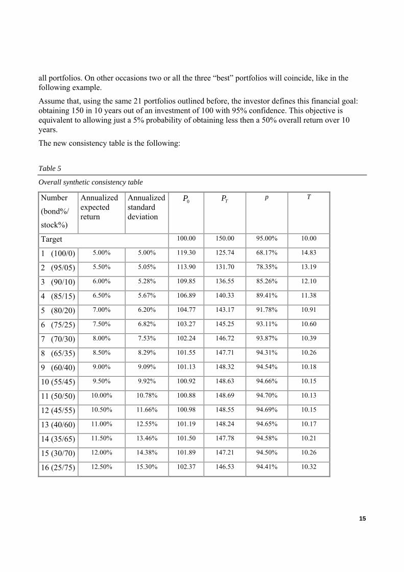
Assume that, using the same 21 portfolios outlined before, the investor defines this financial goal: obtaining 150 in 10 years out of an investment of 100 with 95% confidence. This objective is equivalent to allowing just a 5% probability of obtaining less then a 50% overall return over 10 years.

The new consistency table is the following:

Table 5

Overall synthetic consistency table

Number

(bond%/

stock%)

Annualized expected return

Annualized standard deviation

0P TP p T

Target 100.00 150.00 95.00% 10.00

1 (100/0) 5.00% 5.00% 119.30 125.74 68.17% 14.83

2 (95/05) 5.50% 5.05% 113.90 131.70 78.35% 13.19

3 (90/10) 6.00% 5.28% 109.85 136.55 85.26% 12.10

4 (85/15) 6.50% 5.67% 106.89 140.33 89.41% 11.38

5 (80/20) 7.00% 6.20% 104.77 143.17 91.78% 10.91

6 (75/25) 7.50% 6.82% 103.27 145.25 93.11% 10.60

7 (70/30) 8.00% 7.53% 102.24 146.72 93.87% 10.39

8 (65/35) 8.50% 8.29% 101.55 147.71 94.31% 10.26

9 (60/40) 9.00% 9.09% 101.13 148.32 94.54% 10.18

10 (55/45) 9.50% 9.92% 100.92 148.63 94.66% 10.15

11 (50/50) 10.00% 10.78% 100.88 148.69 94.70% 10.13

12 (45/55) 10.50% 11.66% 100.98 148.55 94.69% 10.15

13 (40/60) 11.00% 12.55% 101.19 148.24 94.65% 10.17

14 (35/65) 11.50% 13.46% 101.50 147.78 94.58% 10.21

15 (30/70) 12.00% 14.38% 101.89 147.21 94.50% 10.26

16 (25/75) 12.50% 15.30% 102.37 146.53 94.41% 10.32

15

17 (20/80) 13.00% 16.23% 102.90 145.77 94.31% 10.38

18 (15/85) 13.50% 17.17% 103.50 144.92 94.21% 10.45

19 (10/90) 14.00% 18.11% 104.16 144.01 94.10% 10.52

20 (05/95) 14.50% 19.05% 104.87 143.04 93.99% 10.60

21 (0/100) 15.00% 20.00% 105.62 142.01 93.88% 10.68

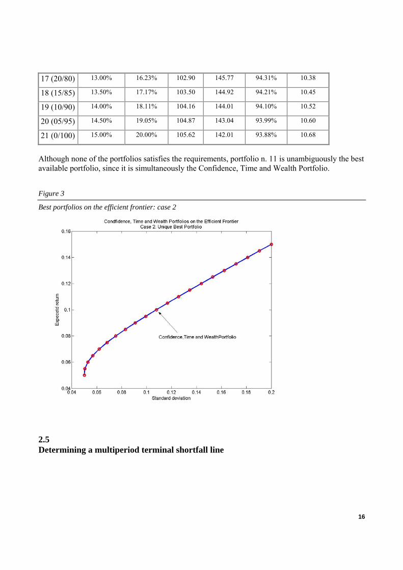
Although none of the portfolios satisfies the requirements, portfolio n. 11 is unambiguously the best available portfolio, since it is simultaneously the Confidence, Time and Wealth Portfolio.

Figure 3

Best portfolios on the efficient frontier: case 2

2.5 Determining a multiperiod terminal shortfall line

16

Given equation (3) ( )TzTWW ipp

T σµ +⋅= exp0

we might be interested in defining a multiperiod shortfall constraint such that, for example, there is a probability no greater than p of obtaining a cumulative return on our investment lower than r,

where r is such that ( )0

1WWr T=+ .

This constraint is based on a multiperiod setting, since time can be considered as one of the variables, and on terminal wealth, since just the final level of wealth is monitored. A shortfall constraint with continuous monitoring of wealth will be outlined in section III.

Imposing the condition:

( ) ( )TzTr ipt σµ +=+ exp1 (8)

and passing to logs we obtain:

TTzr pt σ

µ−+

=)1ln(

(9)

for negative z (low shortfall probabilities) this is a straight line in the µ/σ plane originating from

Trt )1ln( + (which is the average geometric log return implied by the cumulative target arithmetic

return) and slope equal to -T

zσ . Higher target returns will shift the line upwards; higher confidence

levels will increase the slope of the line,

The same constraint can be expressed in terms of terminal minimum wealth:

( ) ( )T

TzWW pT σµ

−−= 0lnln

(10)

Equation (10) can easily be represented graphically in the µ/σ plane. If we go back to the consistency table shown in Table 3 and represent the shortfall line for the stated objectives (initial capital 100, final capital 130, time horizon 10 years and confidence level 0.90) together with the efficient frontier translated to the µ/σ coordinates we obtain the following figure (figure 11).

17

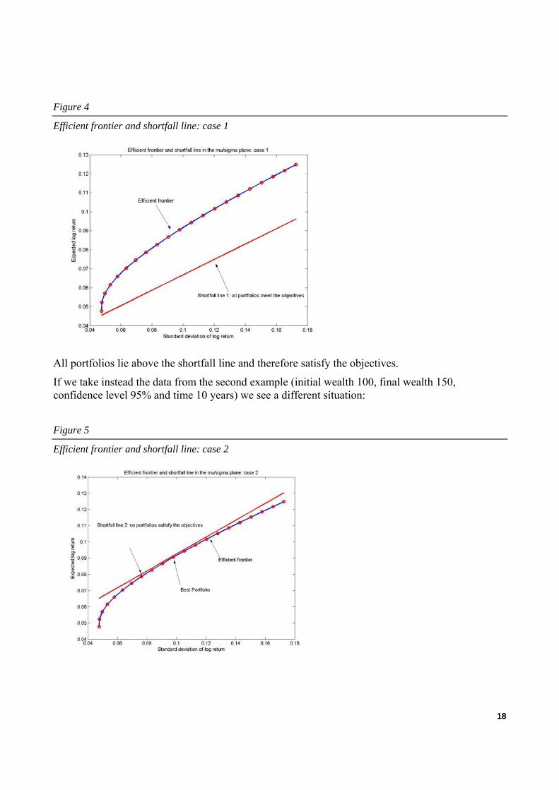
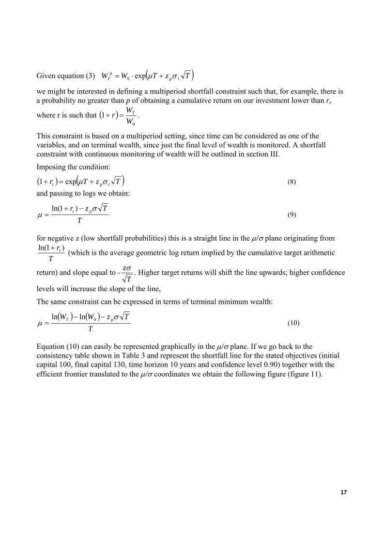
Figure 4

Efficient frontier and shortfall line: case 1

All portfolios lie above the shortfall line and therefore satisfy the objectives.

If we take instead the data from the second example (initial wealth 100, final wealth 150, confidence level 95% and time 10 years) we see a different situation:

Figure 5

Efficient frontier and shortfall line: case 2

18

In this case no portfolio satisfies the objectives: however portfolio 11 (which was the best according to all the three criteria) goes very close to the stated goal and is therefore the closest to the shortfall line.

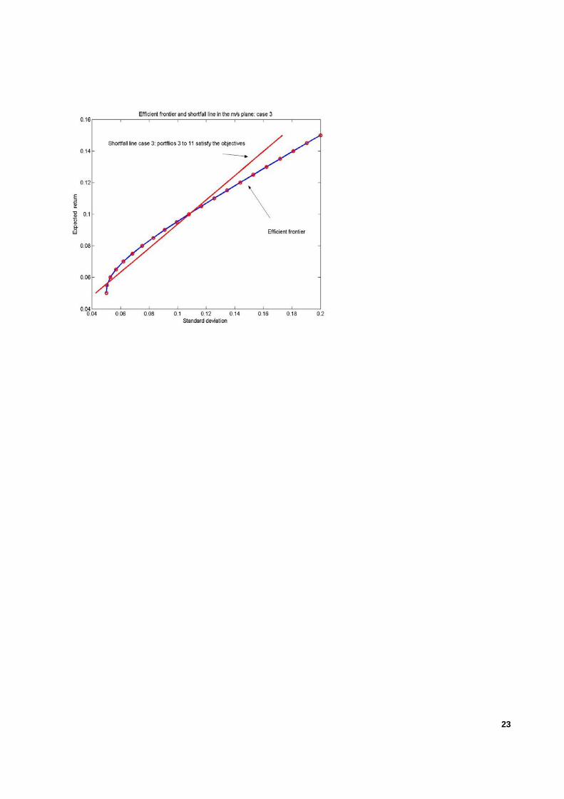
In the two cases shown above either all or none of the portfolios met the stated requirements. Of course this need not always be the case. If for example we use the same efficient frontier and state the following objectives: to obtain a final wealth of 120 out of an initial wealth of 100 in 10 years with 99% confidence, we obtain the following result (figure 13):

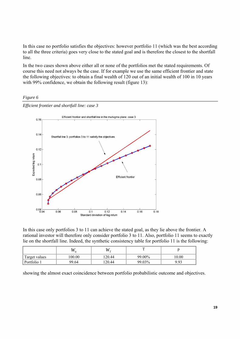
Figure 6

Efficient frontier and shortfall line: case 3

In this case only portfolios 3 to 11 can achieve the stated goal, as they lie above the frontier. A rational investor will therefore only consider portfolio 3 to 11. Also, portfolio 11 seems to exactly lie on the shortfall line. Indeed, the synthetic consistency table for portfolio 11 is the following:

0W TW T p

Target values 100.00 120.44 99.00% 10.00 Portfolio 1 99.64 120.44 99.03% 9.93

showing the almost exact coincidence between portfolio probabilistic outcome and objectives.

19

One of the relevant advantages of this approach is that it allows the simultaneous comparison of different shortfall lines for different time horizons. This holds also for the shortfall line that will be derived in the next section of the paper.

2.6 Representing the (µ,σ) shortfall line in the (m,s) plane

In practical application it might be useful to express the shortfall equation (9) in terms of arithmetic return expected value m and standard deviation s.

First of all we need to convert the standard deviation remembering that:

⎥⎥⎦

⎤

⎢⎢⎣

⎡⎟⎠⎞

⎜⎝⎛+

+=2

11ln

msσ (11)

and:

⎥⎥⎦

⎤

⎢⎢⎣

⎡⎟⎠⎞

⎜⎝⎛+

+−+=−+=22

11ln

21)1ln(

2)1ln(

msmm σµ (12)

Substituting into (9) we obtain

T

Tm

szr

msm

t⎥⎥⎦

⎤

⎢⎢⎣

⎡⎟⎠⎞

⎜⎝⎛+

+−+

=⎥⎥⎦

⎤

⎢⎢⎣

⎡⎟⎠⎞

⎜⎝⎛+

+−+

2

2 11ln)1ln(

11ln

21)1ln( (13)

Rearranging the expression leads to:

( ) ( )( )

( )( )

Tm

smzTsm

mr pt ⎥⎦

⎤⎢⎣

⎡

+++

+⎥⎥⎦

⎤

⎢⎢⎣

⎡

++

+=+ 2

22

22

2

11ln

1

1ln1ln (14)

It’s easier to solve the equation for s as a function of m.

Let’s define R = return relative = 1+m. Equation (14) can be written as:

)1ln(lnln 2

22

22

2

tp rR

sRTzTRsR

R+=

++⋅

⎥⎥⎦

⎤

⎢⎢⎣

⎡⋅

+ (15)

20

which in turn becomes:

)1ln(lnlnln5,0 2

22

2

22

tp rR

SRTzRTR

sRT +=+

+++

− (16)

Now we substitute

xR

sR=

+2

22

ln

and (16) becomes the quadratic equation:

0)1ln(ln5,0 2 =+−++− trRTxTzTx (17)

having solution

[ ]T

rRTTTzTzx tpp

−

+−+±−=

)1ln(ln22

2,1 (18)

substituting back we have:

[ ]2

2

2

22 )1ln(ln2ln

⎪⎭

⎪⎬⎫

⎪⎩

⎪⎨⎧

−

+−+±−=

+T

rRTTTzTz

RsR tpp

(19)

It can be shown that of the 2 possible solutions the correct one has the negative sign before the second square root, from which:

( )[ ]1

)1ln(1ln2exp)1(

22

−⎪⎭

⎪⎬⎫

⎪⎩

⎪⎨⎧

−

+−++−−+=

TrmTTTzTz

ms tpp (20)

This is the expression of the shortfall line in the traditional m,s, plane.

21

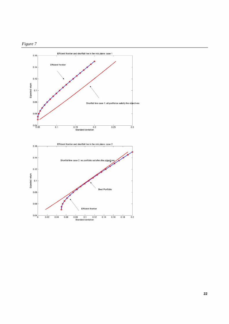
Figure 7

22

23

3. THE DETERMINATION OF A CONTINUOUS SHORTFALL CONSTRAINT

3.1 A continuous-time approach to the Safety-First principle

Investors who have long-term financial objectives rely on time diversification in order to achieve financial goals. Most often, these goals are expressed as objectives to be achieved at a given date. The consistency tables reported in the previous paragraph, for example, stated a deadline for reaching financial goals. Also the shortfall line of equations (18) and (28), although built in a multiperiod setting where time is a variable, just monitors terminal wealth

Most investors, however, might be concerned about the minimum probabilistic level of their wealth during the whole investment period and not just at maturity. There are different reasons why investors could be interested in these values. Although educated about their shortfall risk at maturity, investors might be unaware that most financial investments imply a substantially higher shortfall risk during the life of the investment. Second, it is important that investors facing losses during their investment know what is an “abnormal” loss and what instead lies within predetermined probabilistic boundaries. Finally, investors’ risk tolerance is not independent of financial performance. Endowment effects have been shown to affect investors’ behaviour. Thaler and Johnson2, among others, have shown how investors’ decisions are affected by ongoing performance of their investment. Short-term losses, even if consistent with the achievement of the probabilistic financial objective at maturity, might trigger wrong investment decisions when not panic selling altogether.

It becomes therefore important to assess what is the minimum level of wealth that will be maintained during the whole investment period with a given confidence.

3.2 A dynamic definition of shortfall

The model outlined in part II is suited to deal with this issue.

2 Thaler,Johnson (1990).

24

When equation (12) ( )TzTWW ipp

T σµ +⋅= exp0

is seen as a function of T with given µ, σ and z, we will be able to plot any given quantile of the distribution of wealth over time. We will continue to denote with T the maturity of the investment, while t (with 0<t≤T) will indicate time during the investment process

Safety-first investors will be interested in low quantiles of the distribution of intermediate and terminal wealth, i.e. high confidence levels and negative values of z.

The minimum probabilistic level of wealth over time will be reached when

0=∂∂

tWt and 02

2

>∂∂

tWt (21)

From equation (12) we derive

( )⎟⎟⎠

⎞⎜⎜⎝

⎛+=

∂∂ +

tzeW

tW tztt

20σµσµ (22)

For positive µ, σ and t, the sign of this expression is determined by the sign and level of z, i.e. the parameter associated to the confidence level. If z is positive, i.e. we are considering quantiles greater than 0.5, then the slope is surely positive. If z is negative, however, then the slope can be positive or negative.

For σµ tz 2

−< the slope of the function is negative. This means that, given µ and σ, the p-th

quantile of the wealth probability distribution becomes lower as time increases. Eventually, however, t becomes large enough that for any given negative z the slope will turn back positive.

Given z (22) is equal to 0 when 2

2 ⎟⎟⎠

⎞⎜⎜⎝

⎛−== ∗

µσztt (23)

The second derivative is equal to:

( ) ( )[ ]tt

tzzzttteWtW tztt

4144 2

02

2 −++=

∂∂ + σσµσµσµ (24)

and when t is replaced by t* expression (24) is positive, showing that this is indeed a minimum of the function.

According to (24), the maximum probabilistic loss of any given investment will be reached at a point in time which is proportional to the square of z and to the square of the risk/return ratio.

Of course it might as well be that t* > T. In this case the maximum probabilistic loss would be reached at a time greater than the investment horizon. This means that T is the point in time corresponding to the greatest probabilistic loss, since it still lies on the downward sloping part of

25

the wealth p-th quantile as a function of time. However, if we deal with long-term investment t* will be lower than T unless in the case of abnormally low return/risk ratios.

We can therefore express the point in time corresponding to the highest probabilistic loss as min (t*, T).

If t* < T the minimum probabilistic level of wealth can be determined by replacing (23) in (4)

⎥⎦

⎤⎢⎣

⎡⎟⎟⎠

⎞⎜⎜⎝

⎛−+⋅=

µσσ

µσµ

24exp 2

22

0*zzzWW ipt (25)

which simplifies to:

⎟⎟⎠

⎞⎜⎜⎝

⎛−⋅=

µσ

4exp

22

0*zWWt (26)

so that the maximum probabilistic loss l can be expressed as:

⎥⎦

⎤⎢⎣

⎡⎟⎟⎠

⎞⎜⎜⎝

⎛−−⋅=−=

µσ

4exp1

22

0*0zWWWl t (27)

We can easily check the effectiveness of these equation by applying them to Figure 1, which represented the probabilistic outcome over 10 years of an investment characterized by µ= 10% and σ = 15%. If we are interested in the minimum wealth with 90% confidence then z = norminv (0.10) = -1.2816.

Replacing the values in equation (23) we obtain the timing of the maximum probabilistic loss:

923.010.0*22816.1*15.0 2

=⎟⎠⎞

⎜⎝⎛== ∗tt

Using equation (26) instead we obtain the minimum probabilistic wealth

175.9110.04

15.0)2816.1(exp10022

* =⎥⎦

⎤⎢⎣

⎡⋅

⋅−−⋅=tW

These values can be represented in figure 8, which is an enlargement of figure (1a) in the period 0 – 3 years

26

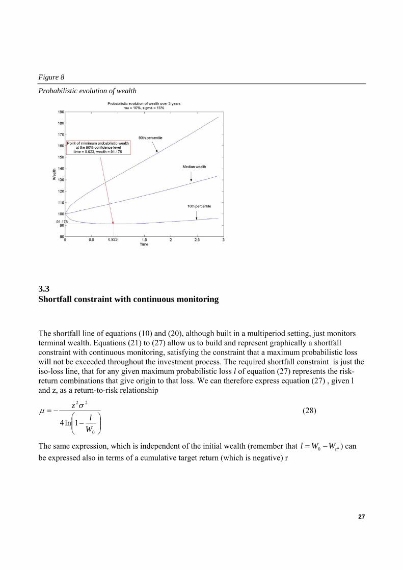
Figure 8

Probabilistic evolution of wealth

3.3 Shortfall constraint with continuous monitoring

The shortfall line of equations (10) and (20), although built in a multiperiod setting, just monitors terminal wealth. Equations (21) to (27) allow us to build and represent graphically a shortfall constraint with continuous monitoring, satisfying the constraint that a maximum probabilistic loss will not be exceeded throughout the investment process. The required shortfall constraint is just the iso-loss line, that for any given maximum probabilistic loss l of equation (27) represents the risk-return combinations that give origin to that loss. We can therefore express equation (27) , given l and z, as a return-to-risk relationship

⎟⎟⎠

⎞⎜⎜⎝

⎛−

−=

0

22

1ln4Wl

z σµ (28)

The same expression, which is independent of the initial wealth (remember that ) can be expressed also in terms of a cumulative target return (which is negative) r

*0 tWWl −=

27

( )rz

+−=

1ln4

22σµ (29)

Unlike the previous traditional terminal wealth shortfall line, which could be defined for any value of r, this continuously monitored shortfall constraint (figure 9), given positive expected returns, is defined and meaningful just for negative values of r (i.e. actual losses). This is because only negative values of r determine a minimum in the probabilistic evolution of wealth.

Figure 9

Continuous shortfall constraint

This continuous-time shortfall line represents risk/return combinations that share the following characteristics: the maximum loss at 95% confidence that can be incurred by investing in these portfolios is 10% of the initial wealth. It is important to remark how these portfolios will produce the maximum probabilistic loss at different points in time (the time at which the maximum probabilistic loss takes place being determined by equation (23)). Once again we can look at Figure 9 to get an insight of this issue: if we take the portfolio having a standard deviation of 10% and a return of 6.42% , this portfolio will have its maximum probabilistic loss of 10% after 1.64 years. On the other hand if we take the portfolio having a standard deviation of 20% and a return of 25.68% it will produce the maximum probabilistic loss of 10% after just 0.41 years. This situation might clash with our intuition that more risky portfolios will exhibit their highest probabilistic loss later than less risky portfolios. This is indeed true in most normal risk-return combinations, when more risky portfolios will imply both higher probabilistic losses and a longer period before these losses are expected. What instead we are considering on the continuous shortfall line are iso-loss portfolios,

28

that is return-risk combinations that produce the same probabilistic maximum loss. In more qualitative terms the economic meaning of the continuous shortfall line is therefore the following: we look for return-risk combinations that produce the same maximum probabilistic loss during the life of the investment. In order for riskier portfolios to yield the same maximum probabilistic loss as less risky portfolios, and not a higher one, the higher volatility must be compensated by a substantial increase in expected return. This means that riskier portfolios will reach the highest probabilistic loss before less risky portfolios.

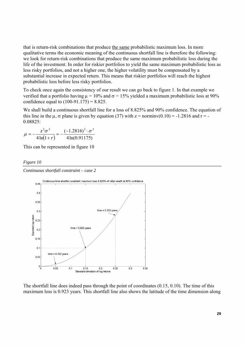
To check once again the consistency of our result we can go back to figure 1. In that example we verified that a portfolio having µ = 10% and σ = 15% yielded a maximum probabilistic loss at 90% confidence equal to (100-91.175) = 8.825.

We shall build a continuous shortfall line for a loss of 8.825% and 90% confidence. The equation of this line in the µ, σ plane is given by equation (37) with z = norminv(0.10) = -1.2816 and r = -0.08825:

( ) )91175.0ln(4)2816.1(

1ln4

2222 σσµ ⋅−−=

+−=

rz

This can be represented in figure 10

Figure 10

Continuous shortfall constraint – case 2

The shortfall line does indeed pass through the point of coordinates (0.15, 0.10). The time of this maximum loss is 0.923 years. This shortfall line also shows the latitude of the time dimension along

29

the line. In order to yield a loss of 8.825% at 90% confidence a portfolio having standard deviation of 5% should have a log return equal to 1.11%; in this case the maximum probabilistic loss could be expected to take place after 8.332 years. On the other hand, always in order to yield a loss of 8.825% at 90% confidence, a portfolio having a standard deviation of 25 % would need a log return of 27.78% and this maximum probabilistic loss would be expected after just 0.332 years.

3.4 The continuous shortfall constraint in the m, s space

Once again it may be more familiar to express the continuous shortfall line in the m,s plane rather than in the µ, σ plane, and just like in the previous line it may be convenient to express s as a function of m.

Remembering that:

⎥⎥⎦

⎤

⎢⎢⎣

⎡⎟⎠⎞

⎜⎝⎛+

+=2

11ln

msσ (11)

and

⎥⎥⎦

⎤

⎢⎢⎣

⎡⎟⎠⎞

⎜⎝⎛+

+−+=−+=22

11ln

21)1ln(

2)1ln(

msmm σµ (12)

equation (36) becomes

)1ln(4

11ln

11ln

21)1ln(

22

2

r

msz

msm

+⎥⎥⎦

⎤

⎢⎢⎣

⎡⎟⎠⎞

⎜⎝⎛+

+

−=⎥⎥⎦

⎤

⎢⎢⎣

⎡⎟⎠⎞

⎜⎝⎛+

+−+ (30)

Rearranging:

⎥⎦

⎤⎢⎣

⎡+

+−

+=

⎥⎥⎦

⎤

⎢⎢⎣

⎡⎟⎠⎞

⎜⎝⎛+

+

21

)1ln(4

)1ln(1

1ln2

2

rz

mm

s (31)

passing to exponential:

1)1(1

2)1ln(2)1ln(42

−+=⎟⎠⎞

⎜⎝⎛+

⎥⎥⎦

⎤

⎢⎢⎣

⎡

−+

+

zrr

mm

s (32)

30

which becomes:

2)1ln(2)1ln(42

2 )1()1(2

mms zrr

+−+= ⎥⎥⎦

⎤

⎢⎢⎣

⎡

−+

++

(33)

and finally:

2)1ln(2)1ln(4

2

)1()1(2

mms zrr

+−+= ⎥⎥⎦

⎤

⎢⎢⎣

⎡

−+

++

(34)

Equation (34) represents the continuous shortfall line in the m,s, plane.

The importance of equation (34) lies in its ability to express the continuous shortfall constraint in the same plane as the one where we traditionally represent efficient portfolios.

3.5 Concluding remarks

Most of the financial planning theory is based on evaluation of terminal wealth within a single-period model. Even when the impact of different time horizons is considered, this is done by comparing the probabilistic terminal outcomes of the investments.

This perspective fails to capture the importance of controlling the maximum probabilistic loss during the investment period. Investments yielding similar probabilistic outcomes can have dramatically different in-period potential loss profiles.

This paper develops a lognormal model in which probabilistic losses are monitored within the whole investment period. Consistently, a continuous shortfall line is developed.

The severe downturn experienced by most equity markets in the period 03/2000 - 03/2003 has highlighted the need to carefully assess intraperiod losses even for investments having supposedly long time horizons. Investors’ risk tolerance evaluation can be seriously affected by past investment outcomes, so that investor behaviour in response to actual portfolio losses can be largely unpredictable. Indeed the evaluation of many investors could be based on a notion of maximum loss not to be exceeded at any point in time during the investment period. A financial planner considering just terminal wealth would therefore be overestimating the investor’s risk tolerance, as intraperiod probabilistic losses might substantially exceed terminal ones.

While time diversification can prove to be largely beneficial to investors, knowing how this diversification effect can show up in time is not irrelevant. In other words the whole investment process is to some extent path dependent, as different paths to the same terminal wealth can determine different investor behaviour. Correct and effective information on the expected risk profile of an investment during its whole life, and not just at maturity, can therefore be valuable in

31

the commercial relationship between promoter/consultant and customer, as it will allow the latter to make a well-informed investment decision.

This aspect can have substantial implications also in terms of regulatory compliance and litigation risk. In the Italian framework, for example, recent litigation issues have involved customers complaining about the short term losses generated by structured notes designed for long-term investment needs. Most capital protection guarantees just consider terminal wealth, so that a substantial effort should be put in disclosing and clearly outlining the financial risk of an investment during its life. The tools developed in the third part of the paper can help in this respect, as they provide a probabilistic representation of the maximum losses that investors might face during the whole life of a financial investment.

32

APPENDIX

Switching between the parameters of the normal and lognormal distribution

The stochastic process describing the evolution of wealth in the model is a Geometric Brownian Motion described by equation (10)

WdZWtdW ση +=

where η is the drift and σ the standard deviation of the process

Returns generated by this process are lognormally distributed with mean m and standard deviation s. Return relatives (1+ return) are as well lognormally distributed with mean (1+m) and standard deviation s.

The natural logarithm of return relatives is normally distributed with mean µ and standard deviation σ.

The following relationships help to switch back and forth from the normal to the lognormal distribution parameters

From lognormal returns to normal return relatives

⎥⎥⎦

⎤

⎢⎢⎣

⎡⎟⎠⎞

⎜⎝⎛+

+=2

11ln

msσ

2

2σηµ −=

2)1ln(

2σµ −+= m

( )( ) ⎥

⎥⎦

⎤

⎢⎢⎣

⎡

++

+=

⎥⎥⎦

⎤

⎢⎢⎣

⎡⎟⎠⎞

⎜⎝⎛+

+−+=22

22

1

1ln1

1ln21)1ln(

sm

mm

smµ

From normal return relatives to lognormal returns

⎟⎟⎠

⎞⎜⎜⎝

⎛+

= 2

2σµ

em

µσµσ 222 22 ++ −= ees

33

Bibliography

ARZAC E.R., BAWA V.S., “Portfolio Choice and Equilibrium in Capital Markets with Safety-First Investors”, Journal of Financial Economics, v. 4, pp. 277-288, 1977.

ATWOOD J., “Demonstrations of the Use of Lower Partial Moments to Improve Safety-First Probability Limits”, American Journal of Agricultural Economics, v. 67, pp. 787-793, 1985.

BAIERL J.T., CHEN P., “Choosing Managers and Funds” Journal of Portfolio Management, V.26, n. 2, pp.47-53. BAUMOL W.J., “An Expected Gain-Confidence Limit Criterion for Portfolio Selection”, Management Science, V. 10,

n. 1, pp.174-182, 1963. BLACK F., LITTERMAN R., “Global Portfolio Optimization”, Financial Analyst Journal, September/October, pp. 28-

43, 1992. BROWNE S., “The Risk and Rewards of Minimizing Shortfall Probability”, The Journal of Portfolio Management,

Summer, pp. 76-85, 1999. CAMPBELL R., HUISMAN R., KOEDIJK K. “Optimal portfolio selection in a Value-at-Risk framework”, Journal of

Banking and Finance, v. 25, pp. 1789-1804, 2001. FROST P.A., SAVARINO J.E., “For Better Performance Constrain Portfolio Weights”, Journal of Portfolio

Management, Fall, pp. 29-34, 1988. GUFFAKER R., “Safety First”, teaching notes, Washington State University, 2003. IBBOTSON R. G., SINQUEFIELD R.A. “Stocks, Bonds, Bills, and Inflation: Simulations of the Future (1976-2000)”,

The Journal of Business, V. 49, n. 3, 1976, pp. 313-338, 1976. JOBSON J.D., KORKIE B.M., “Putting Markowitz Theory to Work”, Journal of Portfolio Management, v.7, Summer

1981, pp. 70-74, 1981. JORION P., “Portfolio Optimization in Practice”, Financial Analyst Journal, v. 48, Jan/Feb, pp. 68-75, 1992. KAPLAN P.D., The Ibbotson-Sinquefield Simulation Made Easy, Ibbotson Working Paper. KATAOKA S., A Stochastic Programming Model, Econometrica, V. 31, n. 1-2, pp. 181-196, 1963. LEIBOWITZ M. L., KOGELMAN S., “Asset allocation under shortfall constraints”, The Journal of Portfolio

Management, Winter, pp. 18-23, 1991. LEWIS A.L., KASSOUF S.T., BREHM R.D., JOHNSTON J., “The Ibbotson-Sinquefield Simulation Made Easy”, The

Journal of Business, V. 53, n. 2, pp. 205-214, 1980. LUCAS A., KLAASSEN P., “Extreme Returns, Downside Risk and Optimal Asset Allocation”, The Journal of

Portfolio Management, Fall, pp. 71-79, 1998. MICHAUD R.O., Efficient Asset Management, Oxford University Press, 1998. MURALIDHAR A., “Optimal Risk-Adjusted Portfolios with Multiple Managers”, Journal of Portfolio Management,

V. 27, n. 3, pp. 97-104, 2001. PYLE D., TURNOVSKY S.J., “Safety-First and Expected Utility Maximization in Mean-Standard Deviation Portfolio

Analysis”, The Review of Economics and Statistics, V. 52, n. 1, pp. 75-81, 1970. ROY A.D., “Safety First and the Holding of Assets”, Econometrica, v. 20, n. 3, pp. 431-449, 1952. TELSER L.G., “Safety First and Hedging”, The Review of Economic Studies, V. 23, n. 1, pp. 1-16, 1955 THALER R., JOHNSON E.J., “Gambling with the house money and trying to break even: the effects of prior outcomes

on risky choices”, Management Science v. 36, pp. 643 – 660, 1990. WILLIAMS J.O., “Maximizing the Probability of Achieving Investment Goals”, The Journal of Portfolio

Management, Fall, pp. 77-81, 1997.

34