On theValidity of Value-at-Risk: Comparative Analyses with ... · 57 On theValidity of Value-at-Risk: Comparative Analyses with Expected Shortfall Yasuhiro Yamai and Toshinao Yoshiba

57

On the Validityof Value-at-Risk:

Comparative Analyseswith Expected Shortfall

Yasuhiro Yamai and Toshinao Yoshiba

Research Division I, Institute for Monetary and Economic Studies, Bank of Japan (E-mail: [email protected], [email protected])

The authors would like to thank Professor Hiroshi Konno (Chuo University) for hishelpful comments. The views expressed herein are those of the authors, and do not necessarily reflect those of the Bank of Japan.

MONETARY AND ECONOMIC STUDIES/JANUARY 2002

Value-at-risk (VaR) has become a standard measure used in finan-cial risk management due to its conceptual simplicity, computationalfacility, and ready applicability. However, many authors claim thatVaR has several conceptual problems. Artzner et al. (1997, 1999),for example, have cited the following shortcomings of VaR: (1) VaRmeasures only percentiles of profit-loss distributions, and thus disregards any loss beyond the VaR level (“tail risk”), and (2) VaR isnot coherent since it is not sub-additive. To alleviate the problemsinherent in VaR, the use of expected shortfall is proposed. In thispaper, we provide an overview of studies comparing VaR andexpected shortfall to draw practical implications for financial riskmanagement. In particular, we illustrate how tail risk can bringserious practical problems in some cases.

Key words: Value-at-risk; Expected shortfall; Tail risk; Sub-additivity

I. Introduction

Value-at-risk (VaR) has become a standard measure used in financial risk manage-ment due to its conceptual simplicity, computational facility, and ready applicability.However, many authors claim that VaR has several conceptual problems.1 Artzner et al. (1997, 1999), for example, have cited the following shortcomings of VaR: (1) VaR measures only percentiles of profit-loss distributions, and thus disregards any loss beyond the VaR level (we call this problem “tail risk”2), and (2) VaR is notcoherent since it is not sub-additive.3

To alleviate the problems inherent in VaR, Artzner et al. (1997) have proposed theuse of expected shortfall.4 Expected shortfall is defined as the conditional expectationof loss given that the loss is beyond the VaR level. Thus, by its definition, expectedshortfall considers the loss beyond the VaR level. Also, expected shortfall is proved tobe sub-additive,5 which assures its coherence as a risk measure. On these grounds,some practitioners have been turning their attention toward expected shortfall andaway from VaR.

In this paper, we provide an overview of studies comparing VaR and expectedshortfall to draw practical implications for financial risk management. Focusing ontail risk, we illustrate how it can bring serious practical problems in some cases.

Our main findings are summarized as follows:(1) Information given by VaR may mislead rational investors who maximize their

expected utility. In particular, rational investors employing only VaR as a riskmeasure are likely to construct a perverse position that would result in a largerloss in the states beyond the VaR level.

(2) Investors can alleviate this problem by adopting expected shortfall as theirconceptual viewpoint, since, by definition, it also takes into account the lossbeyond the VaR level.

(3) The effectiveness of expected shortfall, however, depends on the stability ofestimation and the choice of efficient backtesting methods.

The rest of the paper is organized as follows. Section II gives our definitions and concepts of VaR and expected shortfall. Section III summarizes the criticisms of VaR made by Artzner et al. (1997). Section IV investigates the problem of tail risk in three cases: a portfolio with put options, a credit portfolio, and a portfolio

58 MONETARY AND ECONOMIC STUDIES/JANUARY 2002

1. For other criticisms of VaR, see Artzner et al. (1999), Basak and Shapiro (2001), Danielsson (2001), and Rootzénand Klüppelberg (1999).

2. We have followed the terminology of the BIS Committee on the Global Financial System (2000).3. A risk measure ρ is sub-additive when the risk of the total position is less than or equal to the sum of the risk of

individual portfolios. Intuitively, sub-additivity requires that “risk measures should consider risk reduction byportfolio diversification effects.”

Sub-additivity can be defined as follows. Let X and Y be random variables denoting the losses of two individualpositions. A risk measure ρ is sub-additive if the following equation is satisfied.

ρ(X + Y ) ≤ ρ(X ) + ρ(Y ).

4. The concept of expected shortfall is also mentioned in Artzner et al. (1999), Kim and Mina (2000), and Ulmer(2000).

5. For the proof of sub-additivity of expected shortfall, see the appendix of Acerbi, Nordio, and Sirtori (2001).

dynamically traded in continuous time. Section V examines the applicability ofexpected shortfall to the practice of financial risk management. Section VI lists somecautions when using VaR for risk management. Section VII concludes the paper.

II. Value-at-Risk and Expected Shortfall

This section provides our definitions and concepts of VaR and expected shortfall.

A. Definition of Value-at-RiskVaR is generally defined as “possible maximum loss over a given holding periodwithin a fixed confidence level.” That is, mathematically, VaR at the 100(1 – α ) percent confidence level is defined as the lower 100α percentile6 of the profit-loss distribution (Figure 1).

59

On the Validity of Value-at-Risk: Comparative Analyses with Expected Shortfall

6. Artzner et al. (1999) define VaR at the 100(1 – α ) percent confidence level (VaR α(X )) as follows.

VaR α(X ) = –inf{x |P [X ≤ x ] > α },

where X is the profit-loss of a given portfolio. inf{x |A} is the lower limit of x given event A , and inf{x |P[X ≤ x] > α }indicates the lower 100α percentile of profit-loss distribution. This definition can be applied to discrete profit-lossdistributions as well as to continuous ones. Since the loss is defined to be negative (profit positive), –1 is multiplied to obtain a positive VaR number when one incurs a loss within a given confidence interval.

Using this definition, VaR can be negative when no loss is incurred within the confidence interval because the100α percentile is positive in this case.

Loss

Profit-loss distribution

VaR

α

100 percentileα

Profit

Figure 1 Profit-Loss Distribution and VaR

B. Definition of Expected ShortfallArtzner et al. (1997) have proposed the use of expected shortfall (also called “con-ditional VaR,” “mean excess loss,” “beyond VaR,” or “tail VaR”) to alleviate the problems inherent in VaR.7 Expected shortfall is the conditional expectation of lossgiven that the loss is beyond the VaR level (Figure 2). The expected shortfall isdefined as follows.

The definition of expected shortfallSuppose X is a random variable denoting the profit-loss of a given portfolioand VaRα(X ) is the VaR at the 100(1 – α ) percent confidence level. ESα(X ) isdefined by the following equation.8

ESα(X ) = E [–X |–X ≥ VaRα(X )]. (1)


Loss

Profit-loss distribution

VaR

α

100 percentileα

Expected shortfall

Profit

Conditionalexpectation

Figure 2 Profit-Loss Distribution, VaR, and Expected Shortfall

7. Fishburn (1977), more than 20 years ago, proposed a risk measure similar to expected shortfall. The risk measureproposed by Fishburn (1977) is defined as follows.

Fγ(t ) = ∫ t

–∞(t – x )γdF (x ) γ > 0,

where F (x ) is the distribution function of a random variable denoting profit-loss, t is the target, and γ is the number of moments.

Expected shortfall corresponds to this value if divided by (1 – confidence level) and added to VaR where γ = 1and t = –VaR .

8. E [–X |B ] is the conditional expectation of the random variable –X given event B . Since the profit-loss X is usuallynegative given that the loss is beyond VaR, –X is used for the definition to make expected shortfall a positive number.

C. Calculation of Economic Capital Using VaR and Expected ShortfallVaR is the most popular measure used to calculate economic capital in financial riskmanagement. Furthermore, financial regulators adopt VaR partly to set regulatoryrequirements for capital. The widespread use of VaR for economic capital calculationmay be due to its conceptual simplicity; the economic capital calculated by usingVaR at the 100(1 – α ) percent confidence level corresponds to the capital needed to keep the firm’s default probability below 100α percent. Thus, risk managers cancontrol the firm’s default probability through the use of VaR for risk management.

On the other hand, expected shortfall is defined as “the conditional expectation ofloss given that the loss is beyond the VaR level,” and measures how much one canlose on average in the states beyond the VaR level. Since expected shortfall is by definition more than VaR, economic capital calculation using expected shortfall ismore conservative than that using VaR. However, the figure for economic capital calculated by using expected shortfall is hard to interpret with respect to the firm’sdefault probability. Unlike VaR, expected shortfall does not necessarily correspond tothe capital needed to keep the firm’s default probability below some specified level.

III. Non-Normality and Problems of VaR

Artzner et al. (1997) have cited the following shortcomings of VaR: (1) VaR measuresonly percentiles of profit-loss distributions, and thus it disregards any loss beyond theVaR level, and (2) VaR is not coherent since it is not sub-additive. This section summarizes these criticisms by Artzner et al. (1997). We show that these problemscan be serious when the profit-loss does not obey normal distribution.

A. Risk Measurement with VaR When the Profit-Loss Distribution Is NormalWhen the profit-loss distribution is normal, VaR does not have the problems pointedout by Artzner et al. (1997). First, with the normality assumption, VaR does not havethe problem of tail risk. When the profit-loss distribution is normal, expected shortfall and VaR are scalar multiples of each other, because they are scalar multiplesof the standard deviation.9 Therefore, VaR provides the same information about thetail loss as does expected shortfall. For example, VaR at the 99 percent confidencelevel is the standard deviation multiplied by 2.33, while expected shortfall at thesame confidence level is the standard deviation multiplied by 2.67.

61


9. When the profit-loss distribution is normal, expected shortfall is calculated as follows.

where I {A } is the indicator function whose value is 1 when A is true and 0 when A is false, and qα is the upper100α percentile of standard normal distribution.

For example, from this equation, expected shortfall at the 99 percent confidence level is the standard deviationmultiplied by 2.67, which is the same level as VaR at the 99.6 percent confidence level.

E[–X • I {X ≤ –VaRα(X )}] 1 t 2

ESα(X ) = E[–X |–X ≥ VaRα(X )] = ——————— = – ———— ∫–∞

–VaRα(X)t • e

– ——2σ 2

X dtα ασ X √

–—2π

1 t 2 –VaRα(X ) σXVaRα(X )2 σX

qα2σ

X2

e– ——

2

qα2

= – ———— [–σX2e

– ——2σ 2

X ] = ———e– —–—

2σ 2X

——= ——— e

– ——–2σ 2

X = ———σX ,ασX √

–—2π –∞ α √

–—2π α √

–—2π α √

–—2π

Second, sub-additivity of VaR can be shown as follows. Suppose that there are two portfolios whose profit-loss obeys multivariate normal distribution. With the normality assumption, as we mentioned earlier, VaR is a scalar multiple of the standard deviation, which satisfies sub-additivity.10 Thus, VaR also satisfies sub-additivity.11

Therefore, with the normality assumption, expected shortfall has no advantageover VaR, since VaR satisfies sub-additivity and provides the same information aboutthe tail loss as does expected shortfall.

B. Risk Measurement with VaR When the Profit-Loss Distribution Is NOT Normal

If the profit-loss distribution is not normal, the problems inherent in VaR can beserious. When we cannot assume normality, expected shortfall cannot be generallyrepresented by a function of the standard deviation. Thus, it is not certain whetherVaR provides the same information of the tail loss as does expected shortfall. Weshould calculate expected shortfall as well as VaR to measure the loss beyond the VaRlevel. Furthermore, VaR is not sub-additive in general without normality assumption.

Artzner et al. (1997, 1999) provide two simple cases where the problems inherentin VaR are serious. The first is a short position on digital options, the second is aconcentrated credit portfolio.

Example 1: Short position on digital options12

Consider the following two digital options on a stock, with the same exercise dateT. The first option denoted by A (initial premium u ) pays 1,000 if the value ofthe stock at time T is more than a given U, and nothing otherwise. The secondoption denoted by B (initial premium l ) pays 1,000 if the value of the stock at


10. If two random variables have finite standard deviations, the standard deviations are shown to be sub-additive asfollows.

Let σX and σY be standard deviations of random variables X and Y, and let σXY be covariance of X and Y. SinceσX Y ≤ σXσY , the standard deviation σX +Y of the random variable X +Y satisfies sub-additivity as follows.

——————– ———————σX +Y ≡ √σX

2 + σY2 + 2σXY ≤ √σX

2 + σY2 + 2σXσY = σX + σY .

σXY ≤ σXσY can be proved as follows. Let Z be (Y – µY ) – t (X – µX) for a real value t , where µX and µY are expectations of X and Y.

E [Z 2] = t 2E [(X – µX)2] – 2tE [(X – µX)(Y – µY)] + E [(Y – µY)2].= σX

2t 2 – 2σXY t + σY2

Here, let t be σXY /σX2, then,

σX2σY

2 – σXY2

E [Z 2] = ————— . σX

2

Since E [Z 2] ≥ 0, σXY ≤ σX σY follows.11. To put it more precisely, when the profit-loss distribution is one of the elliptical distribution family and has finite

variance (see Ingersoll [1987] for the definition of the elliptical distribution family), VaR is sub-additive (seeEmbrechts et al. [1999]). The elliptical distribution family includes normal, t , and Pareto distributions.However, for simplicity, we explain the problems of VaR according to whether the distribution is normal.

12. The digital option (also called the binary option) is the right to earn a fixed amount of payment conditional onwhether the underlying asset price goes above (digital call option) or below (digital put option) the strike price.

time T is less than L (with L < U ), and nothing otherwise. Since the payoffs ofthose options are not linear, it is clear that the profit-loss distributions are notnormal even though the price of the underlying assets obeys normal distribution.

Suppose L and U are chosen such that Pr(ST < L ) = Pr(ST > U ) = 0.008,where ST is the stock price at time T. Consider two traders, trader A and trader B,writing one unit of option A and option B, respectively. VaR at the 99 percentconfidence level of trader A is –u , because the probability that ST is more than Uis 0.8 percent, which is beyond the confidence level.13 Similarly, VaR at the 99 percent confidence level of trader B is –l . This is a clear example of the tailrisk. VaR disregards the loss of options A and B, because the probability of theloss is less than one minus the confidence level.

Now consider the combined position on options A and B to show that VaR isnot sub-additive. VaR at the 99 percent confidence level of this combined position (option A plus option B) is 1,000 – u – l , because the probability that ST

is more than U or less than L is 0.016, which is more than one minus the con-fidence level (0.01). Therefore, since the sum of VaR of individual positions(option A and B) is –u – l , it is clear that VaR is not sub-additive (Table 1).

63


Table 1 Payoff and VaR of Digital Options

Stock price Probability Option A Option B Option A + B(percent)

ST < L 00.8 u –1,000 + l –1,000 + u + l

L ≤ ST ≤ U 98.4 u l u + l

U < ST 00.8 –1,000 + u l –1,000 + u + l

VaR –u –l 1,000 – u – l

Example 2: Concentrated credit portfolio Suppose that there are 100 corporate bonds, all with the same maturity of one year. Also suppose that all bonds have a coupon rate of 2 percent, a yield-to-maturity of 2 percent, a default probability of 1 percent, and a recovery rate ofzero.14 Furthermore, it is assumed that the occurrences of defaults are mutuallyindependent.

First, we consider investing US$1 million into 100 corporate bonds, each with an equal amount of US$10,000. Since this portfolio results in a loss if more than one bond defaults in one year,15 the probability of loss is approximately26 percent (1 – the probability that all bonds do not default – the probability that only one bond defaults = 1 – 100 • 0.99100 – 100 • 0.9999 • 0.01). Thus, for thisdiversified investment, VaR at the 95 percent confidence level is positive since the probability of loss is more than 5 percent.

13. See Footnote 6. In this case, VaR is negative because the profit u is guaranteed at the 99 percent confidence level.14. We assume that we incur loss only when the corporate bonds default within the holding period of one year.15. When two corporate bonds default, we lose US$20,000 in principal payments from those two defaulted bonds.

However, we earn US$19,600 in coupon payments from the other 98 non-defaulted bonds. Therefore, the netloss is US$400. If more than two bonds default, the loss is more than US$400.

Second, we consider investing US$1 million into only one of those corporatebonds. For this concentrated investment, we are 95 percent sure that this investment will earn US$20,000, because the default probability is 1 percent.Therefore, VaR at the 95 percent confidence level is –US$20,000. This exemplifiesthe tail risk of VaR, since VaR disregards the potential loss of default. Furthermore,VaR is not sub-additive, because the VaR of the diversified portfolio is larger thanthe VaR of the concentrated portfolio.

As we mentioned earlier, expected shortfall considers the loss beyond the VaRlevel as a conditional expectation. Furthermore, expected shortfall is coherent since itis proved to be sub-additive (Artzner et al. [1997, 1999], Acerbi and Tasche [2001],and Acerbi, Nordio, and Sirtori [2001]). Artzner et al. (1997) have proposed the useof expected shortfall on these grounds.

C. Relevance of the Problems of VaRIn this subsection, we consider whether the problems inherent in VaR are relevant to the practice of risk management. Our main idea is that, while the relevance of sub-additivity may depend on the preferences of risk managers, the tail risk is relevant because it is related to the insolvency of financial institutions, which isamong the central issues of financial risk management.1. Sub-additivityWhether VaR is valid as a risk measure depends on which aspects of risk are relevant to risk managers. A risk measure that considers all relevant aspects of riskwhile ignoring irrelevant ones should be considered appropriate from a practicalstandpoint, because a single risk measure cannot consider all aspects of the profit-loss distribution. Therefore, one should not conclude that VaR is inappropriateonly because it is not sub-additive,16 since sub-additivity itself may be irrelevant for risk managers.

For example, suppose that a firm with total assets of ¥100 million invests all of its assets in two catastrophe bonds:17 bond A, linked to earthquakes in Tokyo, andbond B, linked to earthquakes in Los Angeles. We also assume that all principal and coupon payments of bond A and bond B will be lost in the event of those catastrophes. The question is whether the firm should invest all of its assets in bond A or invest ¥50 million each in bonds A and B. If sub-additivity, or risk reduction by portfolio diversification effect, is considered important, investing ¥50 million each in bond A and bond B is preferred. On the other hand, suppose the firm’s equity capital is less than ¥50 million and the risk manager regards theprobability of default as the most relevant aspect of risk. In this case, investing all ofits assets in bond A is preferred, because the probability that an earthquake will occur


16. Rootzén and Klüppelberg (1999) provide a similar view on sub-additivity.17. Catastrophe bonds are bonds whose coupon and/or principal payments depend on the loss of, or the occurrence

of, a natural catastrophe. Holders of catastrophe bonds can earn a higher coupon because of the inherent reinsurance fee. However, if a predefined catastrophe occurs, all or a part of coupon and principal payments arelost to the bondholders.

either in Tokyo or in Los Angeles is higher than the probability that an earthquakewill occur only in Tokyo.18 For this risk manager, sub-additivity is irrelevant.

However, sub-additivity may be relevant in some cases. For example, Artzner et al.(1997) have cited that, if sub-additivity is not satisfied, a financial institution willonly be able to reduce its required capital by dividing itself into separate institutions.Furthermore, if an initial margin requirement by a futures exchange fails to satisfysub-additivity, futures traders can reduce their initial margin only by dividing theiraccounts into separate accounts. This can be a problem for the futures exchange,because it can be considered a loophole open to futures traders. Moreover, supposethere exists a “conservative” way of aggregating risk simply by summing the VaR ofindividual positions. If VaR is not sub-additive, this “conservative” way is no longerconservative, because the VaR of the total position can be more than the sum of theVaR of individual positions. 2. The problem of tail risk On the other hand, the problem of tail risk is relevant to the practice of risk man-agement, because the loss beyond the VaR level corresponds to the institutional insolvency caused by adverse market conditions. Since the institutional insolvency is the central concern for risk managers and financial regulators, disregarding the loss beyond the VaR level is disregarding the central concern of risk managers andfinancial regulators.19

This leads us to focus on the problem of tail risk in the next section. We emphasize that the problem of tail risk can bring serious practical problems.

IV. Tail Risk of VaR

Basak and Shapiro (2001)20 show that the problem of tail risk can bring the followingpractical problems:

(1) Information given by VaR may mislead investors, because it disregards the lossbeyond the VaR level.

(2) Rational investors employing only VaR as a risk measure are likely to con-struct a perverse position that would result in a larger loss in the states beyondthe VaR level.

They also show that these problems can be especially serious for option portfoliosand credit portfolios. This section illustrates how the tail risk of VaR brings serious practical problems in three cases: an option portfolio, a credit portfolio, and a portfolio dynamically traded in continuous time.

65


18. For example, if the probability that an earthquake occurs in Tokyo and the probability that an earthquake occursin Los Angeles are 1 percent, respectively, and the occurrences are mutually independent, the probability that anearthquake occurs in at least one city, i.e., either Tokyo or Los Angeles, is about 2 percent. Since the firm’s equitycapital is less than ¥50 million, the default probability of the firm when it invests its assets in bonds A and B is 2 percent, while the default probability when it invests all its assets in bond A is 1 percent.

19. See the BIS Committee on the Global Financial System (2000). Furthermore, Federal Reserve ChairmanGreenspan (2000) noted, “In estimating necessary levels of risk capital, the primary concern should be to addressthose disturbances that occasionally do stress institutional solvency—the negative tail of the loss distribution thatis so central to modern risk management.”

20. For the details of Basak and Shapiro (2001), see Subsection IV.C.

A. Option PortfolioThis subsection illustrates the tail risk of VaR with a simple position on a Europeanoption. Suppose that an investor constructs a short position on a European optionwhose maturity is one year. The underlying asset of the option is a stock whose current price and volatility are 100 and 30 percent, respectively. The price of the stock follows a binomial tree process with individual steps of 1/30 year and aprobability of upward movement of 0.6. The premium on the European option is theexpected payoff at maturity with respect to the risk-neutral probability discounted bythe risk-free interest rate.

For simplicity, the investor does not have any financial position other than thisshort position on the one option. The initial premium received from the short posi-tion is invested in a risk-free bond that earns an annual risk-free rate of 5.0 percent.The investor can control only two variables: the strike price of the option and theamount of the option position.

The final profit of this position is the sum of the payoff at maturity of this optionand the future value of the initial premium. Let p (K ) be the put option premiumwith strike price K , Si the stock price at state i , and Pi the subjective probability ofstate i . Furthermore, assume that the utility u (W ) of the investor is represented byu (W ) = lnW, where W is the final wealth, which is the sum of the final profit andthe initial wealth (we assume here that the investor’s initial wealth W0 is 3,000).Then, the expected utility E [u (W )] of the investor is as follows.21

E [u (W )] = ∑Pi• ln{W0 + x • e r • p(K ) – x • max[K – Si, 0]}. (2)

W : Final wealthW0: Initial wealth

VaR is the lower α percentile of the profit-loss distribution of this position,22 andexpected shortfall is the conditional expectation of loss given that the loss is beyondthe VaR level.

We analyze the effect of risk management with VaR and expected shortfall on the rational investor’s optimal decisions by solving the following five optimizationproblems.23

(1) No constraintmaxE [u (W )]. {x, K }


21. E [•] is the expectation operator with respect to the subjective probability. 22. Since the profit-loss distribution in this model is discrete, there may not be any event whose cumulative proba-

bility is equal to 5 percent. Therefore, from the definition in Footnote 6, VaR is calculated as the maximum lossof the states whose cumulative probability is over 5 percent.

23. The minimum and maximum of the strike price are set at 35 and 288, respectively. Those values correspond to theminimum and maximum of the final stock price in our binomial tree model. Furthermore, we constrained theamount of the short position to be less than 60 units so that the final wealth would not be negative in any state.

(2) Constraint with VaR at the 95 percent confidence levelmaxE [u (W )], {x, K }

subject to VaR(95 percent confidence level) ≤ 5.(3) Constraint with expected shortfall at the 95 percent confidence level

maxE [u (W )], {x, K }

subject to expected shortfall(95 percent confidence level) ≤ 7.(4) Constraint with VaR at the 99 percent confidence level

maxE [u (W )], {x, K }

subject to VaR(99 percent confidence level) ≤ 5.(5) Constraint with expected shortfall at the 99 percent confidence level

maxE [u (W )], {x, K }

subject to expected shortfall(99 percent confidence level) ≤ 7.

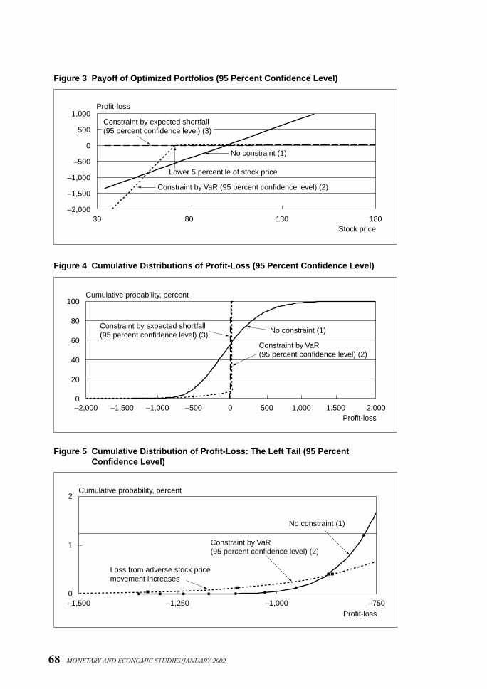
Table 2 shows the results of the optimization problems (1), (2), and (3). The solution with no constraint ([1] in Table 2) consists of selling 21 units of a deep-in-the-money option, while the solution with a 95 percent VaR constraint ([2] in Table 2) consists of selling 60 units of a far-out-of-the-money option. When constrained by VaR, the strike price is set just outside the 95 percent confidenceinterval so that the investor does not incur a large loss within the 95 percent con-fidence interval. However, the loss beyond the VaR level increases due to the increasein the amount of the short position (Figure 3). This implies that, when constrainedby VaR, rational investors optimally construct a perverse position that would result ina larger loss in the states beyond the VaR level.24 On the other hand, the solutionwith a 95 percent expected shortfall constraint ([3] in Table 2) involves little risk,since it consists of selling an insignificant amount of the deep-in-the-money option.

Figures 4 and 5, which show the cumulative profit-loss distribution of solutions(1), (2), and (3), provide further illustrations. With the VaR constraint, the side ofthe distributions (the area between the center and the tail of the distribution)becomes thin to limit VaR by insuring the loss in the normal states. However, the tailof the distributions becomes fat because the investor increases the amount of the

67


24. Ahn, Boudoukh, and Richardson (1999) show that, to minimize the VaR of an option portfolio, it is optimal towrite an out-of-the-money option.

Table 2 Portfolio Profiles (95 Percent Confidence Level)

No constraint (1)Constraint by Constraint by expected

VaR* (2) shortfall** (3)

Position Selling volume 021 060 000.23

Strike price 288 072 288.00

Risk measure VaR 570 005 006.00

Expected shortfall 643 213 007.00

** Optimize with the constraint that VaR at the 95 percent confidence level is less than or equal to 5. ** Optimize with the constraint that expected shortfall at the 95 percent confidence level is less than or equal

to 7.


1,000

500

0

–500

–1,000

–1,500

–2,000

Profit-loss

30 80 130 180Stock price

Constraint by expected shortfall(95 percent confidence level) (3)

No constraint (1)

Constraint by VaR (95 percent confidence level) (2)

Lower 5 percentile of stock price

Figure 3 Payoff of Optimized Portfolios (95 Percent Confidence Level)

100

80

60

40

20

0

Cumulative probability, percent

–2,000 –1,500 –1,000 –500 0 500 1,000 1,500 2,000Profit-loss


No constraint (1)


Figure 4 Cumulative Distributions of Profit-Loss (95 Percent Confidence Level)

2

1

0


–1,500 –1,250 –1,000 –750Profit-loss

No constraint (1)

Loss from adverse stock pricemovement increases


Figure 5 Cumulative Distribution of Profit-Loss: The Left Tail (95 PercentConfidence Level)

short position. On the other hand, with the constraint with expected shortfall, thetail of the distributions becomes thin because the investor decreases the amount ofthe short position to limit the loss beyond the VaR level.

Let us consider whether raising the confidence level of VaR to 99 percent can alleviate this problem. Table 3 shows the results of the optimization problems whenthe confidence levels are raised to 99 percent. The solution with a 99 percent VaRconstraint ([4] in Table 3) consists of selling 60 units of the far-out-of-the-moneyoption, whose strike price is set just outside the 99 percent confidence interval.Again, the loss beyond the VaR level is increased due to the increase in the amount of the short position. Therefore, we cannot mitigate the problem of VaR merely byraising VaR’s confidence level (Figures 3 and 6).

69


1,000

500

0

–500

–1,000

–1,500

–2,000

Profit-loss

30 80 130 180Stock price


No constraint (1)


Lower 1 percentile of stock price

Figure 6 Payoff of Optimized Portfolios (99 Percent Confidence Level)

Table 3 Portfolio Profiles (99 Percent Confidence Level)

No constraint (1)Constraint by Constraint by expected

VaR* (4) shortfall** (5)

Position Selling volume 021 060 000.18

Strike price 288 062 288.00

Risk measure VaR 774 005 007.00

Expected shortfall 816 123 007.00

** Optimize with the constraint that VaR at the 99 percent confidence level is less than or equal to 5. ** Optimize with the constraint that expected shortfall at the 99 percent confidence level is less than or equal

to 7.

This subsection shows how the problem of tail risk brings serious practical problems in a simple option position. Investors can evade risk management with VaRby manipulating the strike price and the amount of the option position. We cannot alleviate this problem merely by raising VaR’s confidence level.

B. Credit PortfolioThis subsection provides a simple illustration of how the tail risk of VaR can bring serious practical problems in credit portfolios. Risk management with VaR may

enhance credit concentration, because VaR disregards the increase of the tail loss dueto credit concentration.

Suppose that an investor invests ¥100 million in the following four mutual funds:(1) concentrated portfolio A, consisting of only one defaultable bond with a 4 percentdefault rate, (2) concentrated portfolio B, consisting of only one defaultable bond witha 0.5 percent default rate, (3) a diversified portfolio that consists of 100 defaultablebonds with a 5 percent default rate, and (4) a risk-free asset. For simplicity, we assumethat the profiles of all bonds in those funds are specified as follows: the maturity is oneyear, the occurrences of default events are mutually independent, the recovery rate is 10 percent, and the yield to maturity is equal to the coupon rate. We further assumethat the yield to maturity, the default rate, and the recovery rate are fixed until maturity. Table 4 shows the specific profiles of bonds included in these mutual funds.


25. The probability that concentrated portfolio A does not default is 0.96 (1 – 0.04), and the probability that concentrated portfolio B does not default is 0.995. Furthermore, the probability that n bonds of the diversifiedportfolio default is 0.05n

• 0.95100–n• 100Cn , where mCn is the number of combinations choosing n out of m. The

probability that both of the concentrated portfolios A and B do not default and n bonds of the diversified portfolio default is the product of those probabilities.

Table 4 Profiles of Bonds Included in the Mutual Funds

Number of Coupon Default rate* Recovery ratebonds included (percent) (percent) (percent)

Concentrated portfolio A 001 4.75 4.00 10

Concentrated portfolio B 001 0.75 0.50 10

Diversified portfolio 100 5.50 5.00 10

Risk-free asset 001 0.25 0.00 —

*The occurrences of defaults are mutually independent.

The probability that both of the concentrated portfolios A and B do not defaultand n bonds of the diversified portfolio do actually default is 0.96 • 0.995 • 0.05n •

0.95100–n •100Cn .25 The probability that both of the concentrated portfolios A and

B default and n bonds of the diversified portfolio default is 0.04 • 0.005 • 0.05n •

0.95100–n •100Cn . Therefore, assuming log utility, the expected utility of the investor is

as follows.

100

E [u (W )] = ∑0.96 • 0.995 • 0.05n • 0.95100–n •100Cn

n=1

1.0475 • X 1 + 1.0075 • X 2 • ln 100 – 0.9n

+ 1.055 • X 3• ————— + 1.0025 • (W0 – X1 – X2 – X3)100

100

E [u (W )] + ∑0.04 • 0.995 • 0.05n • 0.95100–n •100Cn

n=1

1.0475 • 0.1X 1 + 1.0075 • X 2 • ln 100 – 0.9n

+ 1.055 • X 3• ————— + 1.0025 • (W0 – X1 – X2 – X3)100

100

E [u (W )] + ∑0.96 • 0.005 • 0.05n • 0.95100–n •100Cn

n=1

1.0475 • X 1 + 1.0075 • 0.1X 2 • ln 100 – 0.9n

+ 1.055 • X 3• ————— + 1.0025 • (W0 – X1 – X2 – X3)100

100

E [u (W )] + ∑0.04 • 0.005 • 0.05n • 0.95100–n •100Cn

n=1

1.0475 • 0.1X 1 + 1.0075 • 0.1X 2 • ln 100 – 0.9n ,

+ 1.055 • X 3• ————— + 1.0025 • (W0 – X1 – X2 – X3)100

(3)

W : Final wealthW0 : Initial wealthX1 : Amount invested in concentrated portfolio AX2 : Amount invested in concentrated portfolio BX3 : Amount invested in the diversified portfolio

VaR and expected shortfall are calculated according to the definitions in Footnote 6and Subsection II.B, respectively.

We analyze the impact of risk management with VaR and expected shortfall on therational investor’s optimal decisions by solving the following five optimization problems.

(1) No constraintmaxE [u (W )].

{X1, X2, X3}

(2) Constraint with VaR at the 95 percent confidence levelmaxE [u (W )],

{X1, X2, X3}

subject to VaR (95 percent confidence level) ≤ 3.(3) Constraint with expected shortfall at the 95 percent confidence level

maxE [u (W )], {X1, X2, X3}

subject to expected shortfall (95 percent confidence level) ≤ 3.5. (4) Constraint with VaR at the 99 percent confidence level

maxE [u (W )], {X1, X2, X3}

subject to VaR (99 percent confidence level) ≤ 3.(5) Constraint with expected shortfall at the 99 percent confidence level

maxE [u (W )], {X1, X2, X3}

subject to expected shortfall (99 percent confidence level) ≤ 3.5.

71


Tables 5–6 and Figures 7–10 show the results of these optimization problems. Weanalyze the effect of risk management with VaR and expected shortfall by comparingsolutions (2)–(5) with solution (1).


100

80

60

40

20

0


–20 –15 –10 –5 0 5Profit-loss

No constraint (1)

Constraint by expected shortfall (3)

Constraint by VaR (2)

Figure 7 Cumulative Distribution of Profit-Loss (95 Percent Confidence Level)

Table 5 Optimal Portfolios by Each Type of Risk Management (95 Percent Confidence Level)

Risk management Risk management No constraint (1) with VaR* (2) with expected

shortfall** (3)

Portfolio Concentrated portfolio A 07.40 20.10 02.90(percent) (default rate: 4 percent)

Concentrated portfolio B 00.00 00.00 02.00(default rate: 0.5 percent)

Diversified portfolio 92.60 79.90 95.10

Risk-free asset 00.00 00.00 00.00

Risk measure VaR 03.35 03.00 02.75(¥ millions) Expected shortfall 05.26 14.35 03.50

** Optimize with the constraint that VaR at the 95 percent confidence level is less than or equal to 3.** Optimize with the constraint that expected shortfall at the 95 percent confidence level is less than or equal to 3.5.

Table 6 Optimal Portfolios by Each Type of Risk Management (99 Percent Confidence Level)

Risk management Risk management No constraint (1) with VaR* (4) with expected

shortfall** (5)

Portfolio Concentrated portfolio A 07.40 00.70 00.70(percent) (default rate: 4 percent)

Concentrated portfolio B 00.00 18.80 00.50(default rate: 0.5 percent)

Diversified portfolio 92.60 64.90 65.60

Risk-free asset 00.00 15.60 33.20

Risk measure VaR 06.77 03.00 03.13(¥ millions) Expected shortfall 07.83 07.33 03.50

** Optimize with the constraint that VaR at the 99 percent confidence level is less than or equal to 3.** Optimize with the constraint that expected shortfall at the 99 percent confidence level is less than or equal to 3.5.

73


10

5

0


–20 –15 –10 –5Profit-loss

No constraint (1)

Constraint by expected shortfall (3)Constraint by VaR (2)


100

80

60

40

20

0

Cumulative distribution, percent

–20 –15 –10 –5 0 5Profit-loss

No constraint (1)



Figure 9 Cumulative Distribution of Profit-Loss (99 Percent Confidence Level)

5

4

3

2

1

0


–20 –15 –10 –5 0Profit-loss

No constraint (1)




First, we examine the solution of the optimization problem with a 95 percent VaRconstraint ([2] in Table 5). The amount invested in concentrated portfolio A isgreater than that of solution (1), that is, the portfolio concentration is enhanced as aresult of risk management with VaR. The cumulative probability distributions of theprofit-loss of the portfolios in Figures 7 and 8 show how risk management with VaRbrings about this perverse result. When constrained by VaR, the investor has todecrease his investment in the diversified portfolio to reduce the maximum loss witha 95 percent confidence level. The proceeds of the sales of the diversified portfolioshould be invested either in concentrated portfolios or in a risk-free asset.Concentrated portfolio A has little effect on VaR since the probability of default isoutside the 95 percent confidence interval. Thus, the investor optimally chooses toinvest the proceeds in concentrated portfolio A, because this investment ensures ahigher return26 and has little effect on VaR. Although VaR is reduced, this resultwould be considered perverse because of its enhanced concentration and a larger lossin the states beyond the VaR level.

Second, we examine the solution with a 95 percent expected shortfall constraint([3] in Table 5). When constrained by expected shortfall, the investor optimally reallocates his investment to a risk-free asset, substantially reducing the risk of theportfolio. The investor cannot increase his investment in the concentrated portfoliowithout affecting expected shortfall, which considers the loss beyond the VaR level as a conditional expectation. Therefore, unlike risk management with VaR, risk management with expected shortfall does not enhance credit concentration.

The next question we consider is whether raising the confidence level of VaR canbe a solution to the problem. Table 6 shows that, when constrained by VaR at the 99 percent confidence level, the investor optimally chooses to increase his investmentin concentrated portfolio B because the default rate of concentrated portfolio B is 0.5 percent, which is outside the confidence level of VaR. Furthermore, the cumula-tive probability distributions of profit-loss of optimized portfolios (Figures 9 and 10)show that risk management with VaR increases the loss beyond the VaR level. On theother hand, risk management with expected shortfall reduces the potential lossbeyond the VaR level by reducing credit concentration.

This subsection showed that the tail risk of VaR causes failure of credit risk man-agement. VaR can enhance credit concentration, because it disregards the loss beyondthe VaR level. On the other hand, expected shortfall reduces credit concentration,because it considers the loss beyond the VaR level as a conditional expectation.

C. Dynamically Traded PortfolioThis subsection provides the third example, where investors trade two securities (a stockand a bond) dynamically in continuous time. The results and the illustrations in thissubsection are completely dependent on Basak and Shapiro (2001).27


26. The result depends on the return of the concentrated portfolio. If the return of the concentrated portfolio is low,the proceeds are invested in a risk-free asset. That is, whether the risk management with VaR enhances creditconcentration depends on the return of concentrated credits.

27. For the purpose of simple illustration, we have substantially simplified the setting of Basak and Shapiro (2001)and do not provide the detailed derivations of the solutions. See Basak and Shapiro (2001) for further details.

In a general setting where investors trade assets dynamically in continuous time,Basak and Shapiro (2001) show that, if investors are constrained to limit VaR to aspecified level, they optimally choose to construct a position that would result in alarger loss in the states beyond the VaR level. Even though the prices of stocks in thismodel are assumed to follow a geometric Brownian motion (or obey a log-normaldistribution), the profit-loss of the portfolio does not obey a log-normal distribution,because dynamic adjustment of the portfolio creates non-linearity of the final payoff.

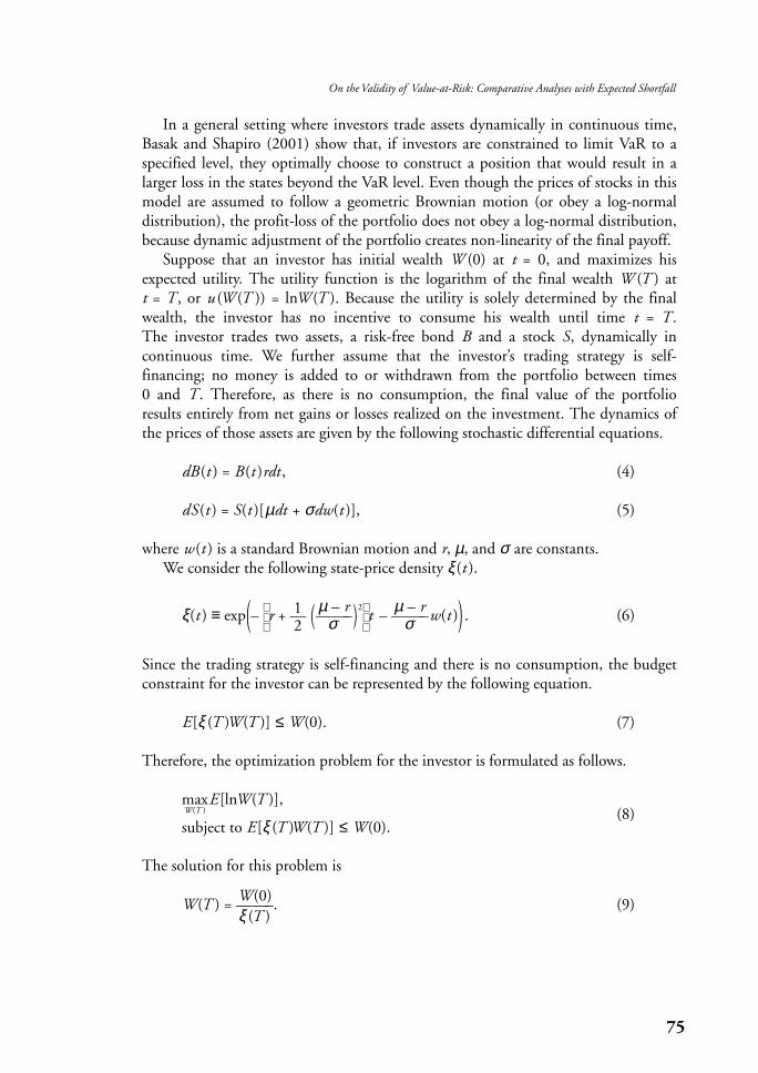
Suppose that an investor has initial wealth W (0) at t = 0, and maximizes hisexpected utility. The utility function is the logarithm of the final wealth W (T ) at t = T , or u (W (T )) = lnW (T ). Because the utility is solely determined by the finalwealth, the investor has no incentive to consume his wealth until time t = T . The investor trades two assets, a risk-free bond B and a stock S, dynamically in continuous time. We further assume that the investor’s trading strategy is self-financing; no money is added to or withdrawn from the portfolio between times 0 and T . Therefore, as there is no consumption, the final value of the portfolioresults entirely from net gains or losses realized on the investment. The dynamics ofthe prices of those assets are given by the following stochastic differential equations.

dB (t ) = B (t )rdt , (4)

dS (t ) = S(t )[µdt + σdw(t )], (5)

where w (t ) is a standard Brownian motion and r, µ, and σ are constants. We consider the following state-price density ξ(t ).

1 µ – r µ – rξ(t ) ≡ exp(– r + — (——–)2 t – ——–w(t )) . (6)

2 σ σ

Since the trading strategy is self-financing and there is no consumption, the budgetconstraint for the investor can be represented by the following equation.

E [ξ (T )W (T )] ≤ W (0). (7)

Therefore, the optimization problem for the investor is formulated as follows.

maxE [lnW (T )], W (T )

subject to E [ξ (T )W (T )] ≤ W (0).(8)

The solution for this problem is

W (0) W (T ) = ——–. (9)ξ (T )

75


Using equations (5), (6), and (9), we obtain

W (0) W (0) ——σ

µ–r

W (T ) = ——– = ———— = A –1 • W (0) • S (T ) , (10)ξ (T ) – ——σ

µ– r

A • S (T )

where A > 0 is constant.Equation (10) shows that the optimal final wealth is a function of the stock price

at maturity. Figure 11 shows the relationship between the optimal final wealth andthe stock price at maturity.


W(T )

S(T )0

W(T ) = A W(0) S(T )–rµσ

Optimal final wealth

Stock price at maturity

Figure 11 Optimal Final Wealth

Let us consider the effect of risk management with VaR on this optimizationproblem. Since VaR is defined as “possible maximum loss over a given holding periodwithin a fixed confidence level,” VaR(α ) with a holding period of T at the 100(1 – α )percent confidence level is defined as follows.

P (W (0) – W (T ) ≤ VaR(α )) ≡ 1 – α . (11)

Here, we formulate risk management with VaR as limiting VaR to being less than orequal to the equity capital.

VaR(α ) ≤ Capital. (12)

Let W–– be the difference between the initial wealth and the equity capital. W–– denotesthe minimum level of final wealth given that the loss is less than the equity capitaland the investor remains solvent. Equation (12) can be reformulated as

VaR(α ) ≤ W (0) – W–– . (13)

From equations (11) and (13), we obtain

P (W (T ) ≥ W–– ) ≥ 1 – α . (14)

This condition shows that to manage risk with VaR is to constrain the probability ofsolvency to be more than 100(1 – α ) percent. Therefore, the optimization problemwith VaR risk management is formulated as follows.

maxE [u (W (T ))], W (T )

subject to E [ξ(T )W (T )] ≤ W (0), (15)P (W (T ) ≥ W–– ) ≥ 1 – α .

Figure 12 illustrates the solution of this optimization problem. To satisfy the VaRconstraint, the final wealth should be more than W–– within a given confidence interval.However, to satisfy the budget constraint, the improvement of final wealth in thosestates must be compensated for by the reduction of final wealth in other states. Thiswould lead to a decrease in final wealth in the states outside the confidence intervalcompared with the optimal solution without a VaR constraint.

77


S(T )


W(T )

0


W

S S

Out of VaR confidence interval:100 percentα

100(1 – ) percentile of stock priceα

Confidence interval of VaR: 100(1 – ) percentα

W(T ) (VaR constraint)

W(T ) (No constraint)Loss out of VaR confidenceinterval increases

Wealth is kept at W in the confidence interval

Figure 12 Optimal Final Wealth with VaR Risk Management

Therefore, rational investors employing VaR as their sole risk measure take a position that would result in a larger loss when the stock price falls below the confidence interval.28

Let us consider the effect of risk management with expected shortfall on theinvestor’s rational decision. For simplicity, we redefine expected shortfall as the conditional expectation of loss given that the loss is beyond some threshold W––.29

We define risk management with expected shortfall as limiting this conditionalexpectation to being less than or equal to some specific constant η, which can beinterpreted as the level of the investor’s equity capital. The formulation is given by

E [W (0) – W (T ) |W (T ) ≤ W–– ] ≤ η. (16)

Let ε ≡ η – W (0) + W–– , then

E [W–– – W (T ) |W (T ) ≤ W–– ] ≤ ε. (17)

For simplicity, Basak and Shapiro (2001) modify equation (17) as follows.30

E [ξ(T )(W–– –W (T ))1{W (T ) ≤W–– }] ≤ ε. (18)

From the definition of the conditional expectation,

E [ξ(T )(W–– –W (T ))1{W (T )≤W–– }]

= E [ξ(T )(W–– – W (T ))|W (T ) ≤ W–– ]P (W (T ) ≤ W–– ). (19)

This equation shows that the left-hand side of equation (18) is the conditional expectation (adjusted by the state price density) multiplied by the probability of loss beyond the threshold. Basak and Shapiro (2001) call the left-hand side of equation (18) “limited expected loss (LEL).” We consider this a variant of expectedshortfall. The optimization problem with constraint by limited expected loss can beformulated as follows.

maxE [u (W (T ))], W (T )

subject to E [ξ (T )W (T )] ≤ W (0), (20)E [ξ(T )(W–– –W (T ))1{W (T )≤W–– }] ≤ ε.


28. Using the general equilibrium framework, Basak and Shapiro (2001) show that the introduction of risk management with VaR would increase stock price volatility in the worst states.

29. If we let W–– = W (0) – VaR (α ), this value corresponds to expected shortfall. However, since VaR (α ) changesaccording to the investor’s trading strategy, the optimization problem becomes intractable if we use originalexpected shortfall as a side constraint. Thus, we set this threshold at a constant W–– .

30. In Equation (18), 1A is the indicator function that takes value 1 if A is satisfied and takes value 0 otherwise.

Figure 13 illustrates the solution of this optimization problem. The investor optimally chooses to decrease the loss beyond the threshold to limit the expectedshortfall. However, with the budget constraint, the final wealth in the better statesdecreases to compensate for the decrease in the loss beyond the threshold. Therefore,risk management with limited expected loss, a variant of expected shortfall, preventsinvestors from taking perverse positions that would result in a larger loss beyond the VaR level.

The result of this subsection implies that the tail risk can bring serious problemswhen investors trade assets dynamically, since they can manipulate the final payoffsof their portfolios through dynamic trading. Furthermore, this shows that the resultin Subsection IV.A of a static option trading strategy generally applies to broad typesof European option instruments, because the payoff of any European-type option canbe replicated by dynamic trading strategies.

79


W(T )

0

W


S(T )

W(T ) (LEL constraint)

W(T ) (No constraint)

Loss in adverse stock price movementdecreases to limit LEL

Upside in favorable stock price movementdecreases because of budget constraint

Threshold of wealth


Figure 13 Optimal Final Wealth with a Constraint by LEL

D. Manipulation of the Tail of DistributionThe illustrations in the previous subsections imply that, if investors can invest inassets whose loss is infrequent but large (such as far-out-of-the-money options orconcentrated credit), the problem of tail risk can be serious. Furthermore, investors can manipulate the profit-loss distribution using those assets, so that the sidebecomes thin and the tail becomes fat (Figure 14). This manipulation of the profit-loss distributions enables investors to decrease VaR without decreasing theirinvestment in risky assets.

Moreover, raising the confidence level of VaR does not solve the problem, becauseinvestors can construct positions that would result in a large loss beyond the newconfidence level. On the other hand, expected shortfall is less likely to provide perverse incentives, since expected shortfall considers the loss beyond the VaR level.

V. Applicability of Expected Shortfall

As we mentioned earlier, at least conceptually, expected shortfall is superior to VaRbecause expected shortfall is less likely to provide perverse incentives to investors.Moreover, Rockafeller and Uryasev (2000) show that portfolio optimization is easierwith expected shortfall than with VaR, because expected shortfall is convex while VaR is not.

However, to apply expected shortfall to the practice of risk management, riskmanagers should weigh the strength and weakness of expected shortfall comparedwith those of VaR (Table 7). From the practical point of view, the effectiveness ofexpected shortfall depends on the stability of estimation and the choice of efficientbacktesting methods.

First, the accurate estimation of the tail of the distribution is especially importantfor the effectiveness of expected shortfall, because expected shortfall considers the lossbeyond the VaR level as a conditional expectation.31 However, the accurate estimation


100 percent

α

Cumulative probability

Expected shortfall(Conditional expectation)

VaR(100 percentile)α

The side of the distribution becomes thin

The tail of the distribution becomes fat

Figure 14 Cumulative Distribution of Profit-Loss When the Tail Risk Occurs

31. Extreme value theory (EVT) can be applied to estimate the tail of distributions. For numerical calculations ofexpected shortfall using EVT, see Neftci (2000) and Scaillet (2000).

of the tail of the distribution is difficult with conventional estimation methods. For example, the correlation among asset prices observed in normal market condi-tions may break down in extreme market conditions. This correlation breakdownwould make it impossible for risk managers to estimate the tail of the portfolioprofit-loss distribution with only conventional Monte Carlo simulations with constant correlation.32

Second, the backtesting of expected shortfall is difficult. The backtesting usingVaR tests the validity of a given model by comparing the frequency of the lossbeyond estimated VaR with the confidence level of VaR. On the other hand, thebacktesting using expected shortfall must compare the average of realized lossesbeyond the VaR level with the estimated expected shortfall. This requires more datathan the backtesting using VaR, since the loss beyond the VaR level is infrequent,thus the average of them is hard to estimate accurately.

VI. Notes of Caution When Using VaR for Risk Management

Although expected shortfall is a conceptually superior risk measure to VaR, the stability of estimation and the choice of efficient backtesting methods are yet to beestablished. Therefore, we presume that VaR will be used as the standard measure in the finance industry. If this is the case, users of VaR such as risk managers andfinancial regulators should be well cautioned concerning the problems of tail risk.This section lists some notes of caution when using VaR for risk management.

A. Relevance of Tail Risk Depends on the Property of the PortfolioGenerally, a single measure cannot represent all aspects of risk. Therefore, risk managers should watch whether the aspects of risk missed by risk measures are relevant to the practice of risk management. We emphasized the problem of tail risk

81


32. Historical simulations may not be able to ensure stable estimation because of insufficient historical data for tail loss.

Table 7 Strength and Weakness of VaR and Expected Shortfall

VaR is:

Strength —Related to the firm’s own default probability

—Easily applied to backtesting—Established as the standard risk

measure and equipped with sufficientinfrastructure (including software andsystem)

Weakness —Unable to consider loss beyond theVaR level (tail risk)

—Likely to give perverse incentives to investors if manipulation of the profit-loss distribution is possible

—Not sub-additive—Difficult to apply to portfolio

optimizations

Expected shortfall is:

—Able to consider loss beyond the VaRlevel

—Less likely to give perverse incentivesto investors

—Sub-additive—Easily applied to portfolio optimizations

—Not related to the firm’s own defaultprobability

—Not easily applied to efficient backtest-ing method

—Not ensured with stable estimation— Insufficient in infrastructure (including

software and system)

because tail risk can bring serious practical problems both for risk managers andfinancial regulators.

Section IV shows that the tail risk is serious when investors have an opportunityto invest in assets whose loss is infrequent but large. Option and credit portfolios aretypical of such vulnerable portfolios. Risk managers and financial regulators shouldbe cautioned when dealing with those kinds of portfolios.

B. Risk Management with VaR May Give a Perverse Incentive to Rational Investors

Section IV showed that, if investors have an opportunity to invest in assets whose lossis infrequent but large, the investors can reduce VaR by manipulating the profit-loss distributions. Furthermore, rational investors employing only VaR as a risk measure are likely to construct a perverse position that would result in a largerloss in the states beyond the VaR level. Raising the confidence level of VaR cannotsolve this problem.

Therefore, users of VaR, such as risk managers and financial regulators, should bealways reminded of the perverse incentives provided by VaR, and should implementcomplementary measures if necessary.

C. Implications for Stress TestsThe BIS Committee on the Global Financial System (2000) summarizes how stresstests are used in internationally active financial institutions as follows.

(1) Comparative analyses between the firm’s risk-taking and risk appetite“Stress tests produce information summarising the firm’s exposure to extreme,but possible, circumstances. Risk managers at interviewed firms frequentlydescribed their roles within firms as assembling and summarising informationto enable senior management to understand the strategic relationship betweenthe firm’s risk-taking (such as the extent and character of financial leverageemployed) and risk appetite.”

(2) Measurement of tail risk“If large losses carry an especially heavy cost to the firm, senior managementmay use stress tests to guide the firm away from risk profiles with excessive tail risk.”

Conventional practices of stress tests such as calculating VaR at a high confidencelevel (for example, 99.99 percent) or calculating extreme loss with historical or hypothetical stress scenarios may be appropriate for the first purpose (i.e., analysescomparing the firm’s risk-taking and risk appetite). However, those conventionalmethods are not appropriate for the second purpose (measuring tail risk), becausethey are based solely on the single point of profit-loss distributions. Traders can evade risk limits calculated by the conventional stress tests by taking an excessive risk beyond this point. To measure the portfolio’s vulnerability to tail risk, risk managers should adopt risk measurement methods that can incorporate information concerning the tail, typically risk measurement with expected shortfall.


D. Importance of Adequate Risk Management at the Desk LevelSome practitioners may counter the criticisms of VaR, saying, “At the trading desklevel, we do not rely solely on VaR. Risks are managed with numerous quantitativeand qualitative measures such as detailed monitoring of the profit-loss diagrams ofindividual positions. Thus, the tail risk can be managed adequately with those conventional risk management practice at the desk level.”

The validity of this view depends on whether adequate tail risk management atthe desk level ensures adequate tail risk management at the companywide level. If thisdoes not hold, the validity of the practitioner’s view would be seriously questioned.We can infer the validity of this view using sub-additivity of expected shortfall. Sinceexpected shortfall is sub-additive, expected shortfall of the total position is no morethan the sum of expected shortfall of the individual positions. If we can considerexpected shortfall to represent the tail risk, adequate risk management at the desklevel ensures appropriate risk management at the companywide level. This suggeststhe necessity and the effectiveness of adequate risk management at the desk level.

E. Importance of Managing Credit ConcentrationSubsection IV.B showed that credit concentration plays the main role in the tail risk of credit portfolios. Credit Suisse Financial Products (1997) notes that credit riskmanagement beyond the VaR level should be “quantified using scenario analysis andcontrolled with concentration limits.” When we use VaR for the risk management of credit portfolios, we should ensure that credit concentration is limited by complementary measures, since VaR disregards the increase of the potential loss due to credit concentration.

VII. Concluding Remarks

We considered the validity of VaR as a risk measure by comparing it with expectedshortfall. We emphasized the problem of tail risk, or the problem that VaR disregardsthe loss beyond the VaR level. This problem can bring serious practical problems,because information provided by VaR may mislead investors. Investors can alleviatethis problem by adopting expected shortfall, since it also considers the loss beyond theVaR level. However, the effectiveness of expected shortfall depends on the stability ofestimation and the choice of efficient backtesting methods. Risk managers shouldweigh the strength and weakness of expected shortfall before adopting it as part ofthe practice of risk management.

There are several outstanding issues for further research other than the problemsof the stable estimation and the efficient backtesting of expected shortfall. Among the most important issues is how to identify portfolios vulnerable to the tail risk efficiently. If we know how to identify vulnerable portfolios, we are able to managetail risk efficiently by implementing complementary measures such as calculation of expected shortfall only to those vulnerable portfolios. Section IV provides an intuitive answer to this question; a portfolio that includes assets whose loss is large but infrequent is vulnerable to tail risk because investors can manipulate the

83


profit-loss distributions. This answer may not be sufficient for risk managers, becauseit does not answer how large is “large” enough or how infrequent is “infrequent”enough for tail risk to bring serious practical problems. Therefore, we hope thatfuture research will provide us with more rigorous guidance on how to identify vulnerable portfolios.


Acerbi, C., C. Nordio, and C. Sirtori, “Expected Shortfall as a Tool for Financial Risk Management,”working paper, Italian Association for Financial Risk Management, 2001.

———, and D. Tasche, “On the Coherence of Expected Shortfall,” working paper, Center forMathematical Sciences, Munich University of Technology, 2001.

Ahn, D., J. Boudoukh, and M. Richardson, “Optimal Risk Management Using Options,” The Journalof Finance, 54 (1), 1999, pp. 359–375.

Artzner, P., F. Delbaen, J. M. Eber, and D. Heath, “Thinking Coherently,” Risk, 10 (11), 1997, pp. 68–71.

———, ———, ———, and ———, “Coherent Measures of Risk,” Mathematical Finance, 9 (3),1999, pp. 203–228.

Basak, S., and A. Shapiro, “Value-at-Risk Based Risk Management: Optimal Policies and Asset Prices,”The Review of Financial Studies, 14 (2), 2001, pp. 371–405.

BIS Committee on the Global Financial System, “Stress Testing by Large Financial Institutions:Current Practice and Aggregation Issues,” No. 14, 2000.

Credit Suisse Financial Products, Credit Risk+: A Credit Risk Management Framework, 1997. Danielsson, J., “The Emperor Has No Clothes: Limits to Risk Modelling,” working paper, Financial

Markets Group, London School of Economics, 2001. Embrechts, P., A. McNeil, and D. Straumann, “Correlation and Dependency in Risk Management:

Properties and Pitfalls,” preprint, ETH Zürich, 1999. Fishburn, P. C., “Mean-Risk Analysis with Risk Associated with Below-Target Returns,” American

Economic Review, 67 (2), 1977, pp. 116–126. Greenspan, A., “Banking Evolution,” remarks at the 36th Annual Conference on Bank Structure

and Competition of the Federal Reserve Bank of Chicago (http://www.federalreserve.gov/boarddocs/speeches/2000/20000504.htm), 2000.

Ingersoll, J. E., Jr., Theory of Financial Decision Making, Rowman & Littlefield Publishers, 1987.Kim, J., and J. Mina, RiskGrades Technical Document, RiskMetrics Group, 2000. Neftci, S. N., “Value at Risk Calculations, Extreme Events, and Tail Estimation,” Journal of Derivatives,

7 (3), 2000, pp. 23–37. Rockafeller R. T., and S. Uryasev, “Optimization of Conditional Value-at-Risk,” Journal of Risk, 2 (3),

2000, pp. 21–41. Rootzén, H., and C. Klüppelberg, “A Single Number Can’t Hedge against Economic Catastrophes,”

Ambio, 26 (6), 1999, pp. 550–555. Scaillet, O., “Nonparametric Estimation and Sensitivity Analysis of Expected Shortfall,” working paper,

IRES, 2000. Ulmer, A., “Picture of Risk,” technical document, RiskMetrics Group, 2000.

85


References


Documents

On theValidity of Value-at-Risk: Comparative Analyses with ... · 57 On theValidity of Value-at-Risk: Comparative Analyses with Expected Shortfall Yasuhiro Yamai and Toshinao Yoshiba