Combustion Chemistry - Princeton University

Combustion Chemistry

Hai Wang Stanford University

2015 Princeton-CEFRC Summer School On Combustion Course Length: 3 hrs

June 22 – 26, 2015

Copyright ©2015 by Hai Wang This material is not to be sold, reproduced or distributed without prior written

permission of the owner, Hai Wang.

1-1

Lecture 1

1. THERMOCHEMISTRY Thermodynamics is the foundation of a large range of physical science problems. It provides us with a basic understanding about the driving force of a physical process and the limits of such a process. The development of thermodynamic theory was intimately related to combustion. In particular, the second law of thermodynamics was conceived largely to prove that it is impossible to operate a perpetual motion machine. 1.1 Thermodynamic First Law The first law of thermodynamics states that the energy is conserved when this energy is transformed from one form to another. In the context of combustion analysis, we state that for a control mass (or the working fluid), Q −W = ΔU (1.1)

where Q (kJ or kcal) is the heat transferred from the working fluid to the surrounding, W (kJ or kcal) is the work done by the working fluid to the surrounding, and U (kJ or kcal) is the internal energy of the working fluid. It is important to mention that energy transformation always involves a process that has a initial state (1) and a final state (2). ΔU = U2 – U1 is therefore the change of internal energy of the working fluid from the initial state to the final state. Thermodynamic analysis follow the convention that if the working fluid gives off heat to the surrounding, Q < 0 , and if the working fluid receives heat from the surrounding, Q is positive. For example, in a simple cooling process, a fluid loses its internal energy to the surrounding (i.e., lowering its temperature) and thus ΔU < 0. Assuming that no work is done (W = 0), then Q < 0. Likewise, if the working fluid does net work to the surrounding, W is positive, and if the surrounding does net work to the working fluid, W < 0 (e.g., for adiabatic compression (Q = 0), the work done by the surrounding to the working fluid serves to raise the internal energy of the working fluid, since –W = ΔU > 0. The symbol U designates the internal energy of a given mass of a substance. Internal energy is a measure of the total energy of the control mass. For example, excluding nuclear energy the internal energy of air is a sum of the kinetic energy of each atom. Therefore, the internal energy can be made a material property if it is defined as the internal energy per mass, an intensive property, denoted here as u (kJ/kg) or u (kJ/kmol). In this course, we shall follow the notation that intensive properties are expressed in lower cases. Assuming that we are running a thermodynamic process that the only work done during the process is that associated with boundary work under a constant pressure P1 = P2 = P (e.g., a piston work), the work done may be calculated from

Stanford University ©Hai Wang Version 1.2

1-2

= = −∫2

2 11( )W PdV P V V . (1.2)

Putting Eq. (1.2) into Eq. (1.1), we have Q = U2 + P2V2( )− U1 + P1V1( ) , (1.3) where V is the volume of the working fluid. In this case, the heat transferred during the process corresponds to a net change of the controlled mass in the quantity U + PV between the initial and final states. We find it convenient to define a new thermodynamic property, the enthalpy = +H U PV , (1.4a) = +h u Pv , (1.4b) = +h u Pv . (1.4c) Here v and v are the specific volumes, having the units (m3/kg) and (m3/kmol) respectively. Clearly, these specific volumes are related to the mass density ρ and molar density (or concentration) c, respectively, i.e., v = 1/ρ and v = 1/c. In general, the internal energy u and enthalpy h depend on only two independent properties that specifying the thermodynamic state, e.g., (T, P), (T, v), or (P, v). For a low-density gas like air or combustion gases, T, P, and v are related by the ideal gas law or the equation of state, = 'Pv RT , (1.5a) = uPv R T , (1.5b) where Ru is the universal gas constant (8.314 kJ/kmol-K), R’ is the specific gas constant and equal to Ru/MW, and MW is the molecular weight of the substance. For a low-density gas, the internal energy is primarily a function of T, i.e., ≅ ( )u u T . This

relationship may be expressed by defining a constant-volume specific heat vc (kJ/kmol-K)

∂⎛ ⎞= ⎜ ⎟∂⎝ ⎠v

v

uc

T . (1.6)

For an ideal gas we have = vdu c dT . Likewise, the relationship between enthalpy and temperature may be established by defining a constant-pressure specific heat pc (kJ/kmol-K)

c p =∂h∂T

"

#$

%

&'p

, (1.7)


1-3

and = pdh c dT . In other words, the two specific heats defined above characterize the heat required to raise the temperature of a substance by 1 K. Since for an ideal gas

= + = +( ) udh du d pv du R dT and ≅ ( )u u T , we see that h and pc are also function of temperature only. The relation between dh and du also yields = +p v uc c R . Here it is important to note that the enthalpy discussed thus far involves only the heating or cooling a substance. This type of enthalpy is known as the sensible enthalpy or sensible heat. Later, we will introduce two other types of enthalpy, one of which is critical to combustion problems. The first law of thermodynamics is quite insufficient to describe energy conversion. Equation (1.1) states that it is possible to cool a substance of a given mass spontaneously (i.e., lowering its internal energy U), and transfer this energy to the surrounding. In other words, within the first law of thermodynamics, it is possible to transform heat from a low-temperature body to a high temperature body. We know that this cannot be true. The second law of thermodynamics, to be discussed below, will address this problem. 1.2 Thermodynamic Second Law and Entropy In contrast to the first law of thermodynamics, the second law is more difficult to understand. The Kelvin-Planck statement of this law is It is impossible to construct a device that will operate in a cycle and produce no effect other than the raising of a weight and the exchange of heat with a single reservoir. In other words, it is impossible to construct a heat engine that (a) receives heat continuously from a heat reservoir, (b) turns the heat transferred entirely to work, (c) without having to leave any marks on the surrounding. Without diverging into a lengthy discussion of the second law of thermodynamics, let us define entropy S (kJ/K) as

δ⎛ ⎞= ⎜ ⎟⎝ ⎠int revQ

ST

. (1.8)

where (δQ)int rev is the heat a control mass received during an infinitesimal, internally reversible process. Based on an analysis of thermodynamic cycles, it may be shown that for a spontaneous process to occur, the entropy of the control mass must be equal to or greater than zero, ΔS = S2 – S1 ≥ 0. (1.9) Neither the Kelvin-Planck statement nor Eq. (1.8) really tells us what entropy is. An understanding of entropy will have to come sometime later when we introduce statistical thermodynamics. Here let us place some discussion about entropy in a non-rigorous fashion. Entropy is a measure of molecular randomness. This randomness may be measured by the predictability of the positions of atoms in a substance. A crystal material would have a small entropy because atoms are more or less “locked” into the crystal lattice. In fact, the third law of thermodynamics states that the entropy of a pure crystalline substance at absolute


1-4

zero temperature is zero. In other words, the atoms in a pure crystal are “frozen” (no oscillation) at 0 K. Therefore, their spatial position is completely predictive. In contrast, a gas would have a large entropy because molecules that make up the gas constantly move about in the space, resulting in small predictability regarding their positions. Moreover, an increase in temperature of the gas leads an increase in the speed of molecular motion and smaller predictability of the molecular positions. In other words, entropy increases with an increase in temperature. In contrast, an increase in pressure leads to closer spacing among molecules. As a result, the molecules become more confined spatially and the entropy is smaller at higher pressures. The dissociation of a chemical substance into gaseous fragments always leads to an increase in entropy since it is harder to predict the spatial positions of the fragments than the molecules of their parent substance. The inequality expressed by Eq. (1.9) basically says that for a spontaneous process to occur, the entropy of the control volume must increase, i.e., natural processes favor more randomness than orderness. Conceptually this makes sense since our experience tells us that a building can spontaneously collapse into a pile of rubble, but a pile of rubble would not spontaneously transform into a building (not without our intervention). Two different gases, say, N2 and O2, would always mix and they never spontaneously separate spatially, leading to better predictability of their positions. The concept of entropy is also deeply rooted in our life. Take the life of a workaholic as an example, the first law of thermodynamics states that it is possible for him/her to receive heat Q in the form of food and hopefully without gaining weight (ΔU = 0), to transform this heat entirely to work W. The second law says that he/she really cannot do this. That is, my office always gets messier over time and I will need to clean it (i.e., not all the heat goes to useful work) as time goes by. Because entropy is a measure of randomness, which in turn, is determined by T and P, it is also a material property. It follows that we can define and denote the entropy of a substance by s (kJ/kg-K) or s (kJ/kmol-K). Although we do not know for the time being how to directly measure entropy, we may develop some relationships that can help us to determine the entropy value. Here we apply the first law to a constant T and P, internally reversible process (e.g., compress a volume immersed in a temperature bath by a piston very slowly), δ δ− =int rev int rev ,Q W dU (1.10) but since δ =int revQ TdS and δ =int revW PdV , we have = +TdS dU PdV (1.11) or

= + = +v

du Pdv dT Pdvds c

T T T T . (1.12)


1-5

Replacing u by −h Ts and rearranging, we obtain

= − = −p

dh vdP dT vdPds c

T T T T . (1.13)

Applying the ideal gas law, we may rewrite equations (12) and (13) as

= +v u

dT dvds c R

T v , (1.14)

= −p u

dT dPds c R

T P . (1.15)

One may integrate the above equations to show that

Δ = − = +∫2

22 1 1

1

lnv u

vdTs s s c R

T v , (1.16)

Δ = − = −∫2

22 1 1

1

lnp u

PdTs s s c R

T P . (1.17)

Equation (1.17) states that if pc is a constant, an increase of temperature by ΔT from T causes the entropy to increase by ( )+ Δln 1pc T T and an increase of pressure by ΔP from P leads to the entropy to decrease by ( )+Δln 1uR P P . Given the third law of thermodynamics, which establish the absolute zero for entropy, the entropy of an ideal gas at a given thermodynamic state (i.e., known T and P) can be easily determined if pc is known. Equation (1.17) also states that unlike enthalpy and internal energy, the entropy of an ideal gas is a function of both temperature and pressure. In application, we define the standard entropy os as

( ) ( )⎡ ⎤ ⎡ ⎤Δ = − = = − − −⎢ ⎥ ⎢ ⎥⎣ ⎦ ⎣ ⎦∫ ∫ ∫o oo o o2 12

2 1 1 0 0ln ln

T T

p p u p u

dT dT dTs s s c c R P c R P

T T T , (1.18)

or

( )= −∫o o

0ln

T

p u

dTs c R P

T , (1.19a)

where oP is the standard pressure of 1 atm. Hence,

0

T

p

dTs c

TΔ = ∫o , (1.19b)


1-6

By tabulating this standard entropy, we may easily determine the entropy change of an ideal gas under an arbitrary condition by

( ) ( )= −oo, lnu

Ps T P s T R

P . (1.20)

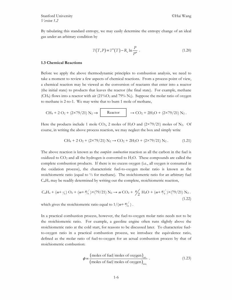
1.3 Chemical Reactions Before we apply the above thermodynamic principles to combustion analysis, we need to take a moment to review a few aspects of chemical reactions. From a process point of view, a chemical reaction may be viewed as the conversion of reactants that enter into a reactor (the initial state) to products that leaves the reactor (the final state). For example, methane (CH4) flows into a reactor with air (21%O2 and 79% N2). Suppose the molar ratio of oxygen to methane is 2-to-1. We may write that to burn 1 mole of methane,

CH4 + 2 O2 + (2×79/21) N2 → → CO2 + 2H2O + (2×79/21) N2 .

Here the products include 1 mole CO2, 2 moles of H2O and (2×79/21) moles of N2. Of course, in writing the above process reaction, we may neglect the box and simply write CH4 + 2 O2 + (2×79/21) N2 → CO2 + 2H2O + (2×79/21) N2 . (1.21) The above reaction is known as the complete combustion reaction as all the carbon in the fuel is oxidized to CO2 and all the hydrogen is converted to H2O. These compounds are called the complete combustion products. If there is no excess oxygen (i.e., all oxygen is consumed in the oxidation process), the characteristic fuel-to-oxygen molar ratio is known as the stoichiometric ratio (equal to ½ for methane). The stoichiometric ratio for an arbitrary fuel CmHn may be readily determined by writing out the complete, stoichiometric reaction,

CmHn + (m+ 4n ) O2 + (m+ 4

n )×(79/21) N2 → m CO2 + 2n H2O + (m+ 4

n )×(79/21) N2 .

(1.22) which gives the stoichiometric ratio equal to 1/(m+ 4

n ) .

In a practical combustion process, however, the fuel-to-oxygen molar ratio needs not to be the stoichiometric ratio. For example, a gasoline engine often runs slightly above the stoichiometric ratio at the cold start, for reasons to be discussed later. To characterize fuel-to-oxygen ratio in a practical combustion process, we introduce the equivalence ratio, defined as the molar ratio of fuel-to-oxygen for an actual combustion process by that of stoichiometric combustion:

( )( )

φ = act.

stoi.

moles of fuel moles of oxygen

moles of fuel moles of oxygen . (1.23)

Reactor


1-7

Of course, it may be shown that the equivalence ratio may be calculated using the molar ratio of fuel-to-air or the mass ratio of fuel-to-oxygen or fuel-to-air. By examining the equivalence ratio, we can quickly tell the nature of the fuel/air mixture. That is, if φ = 1, we have stoichiometric reaction; if φ < 1 we have excess oxygen that is not completely used in a reaction process and the combustion is called fuel-lean combustion; if φ > 1 we have excess fuel and the combustion is called fuel-rich combustion.

1 fuel lean

1 stoichiometric

> 1 fuel rich

φ<⎧⎪= ⎨⎪⎩

Under the fuel rich combustion, the combustion reaction inherently yields incomplete combustion products, like CO, H2 etc. 1.4 Enthalpy of Formation, Enthalpy of Combustion As we discussed in section 1.1, there are 3 types of enthalpy. The first type is associated with heating or cooling of a substance. The second type is latent enthalpy (or heat). This is the enthalpy associated with the phase change of a substance. For example, the latent heat of evaporation of H2O, lgh , is = −lg g lh h h , (1.24)

where gh and lh are the enthalpy of water in its vapor and liquid states, respectively. What is perhaps more important to combustion analysis is the reaction enthalpy. For example, reaction (21) releases an amount of heat due to chemical bond rearrangements. Combining Eqs (1.3) and (1.4a), we have = −2 1Q H H .

Since state 1 corresponds to the reactants, and state 2 corresponds the products, the above equation states that (a) in a non-adiabatic reactor, the heat released from the reactor is equal to the total enthalpy of the combustion products subtracted by the total enthalpy of the reactant, and (b) since for a combustion process Q < 0, H2 < H1, i.e., the total enthalpy of the products is lower than that of the reactants. The nature of reaction enthalpy is very different from the sensible enthalpy, as the former is due to re-arranging chemical bonds and the latter is simply due to heat and cooling without changing the chemical nature of the substance. To calculate the exact amount of reaction enthalpy and therefore the amount of heat release, we need to first understand the concept and application of enthalpy of formation.


1-8

The enthalpy of formation h f at a given temperature is defined as the heat released from producing 1 mole of

a substance from its elements at that temperature. By this definition, the enthalpy of formation is zero for the reference elements. These elements are, for example, graphite [denoted by C(S) hereafter), molecular hydrogen H2, molecular oxygen (O2), molecular nitrogen (N2), and molecular chlorine (Cl2). The enthalpy of formation of CO2, say at 298 K, may be conceptually measured by reacting 1 mole of graphite and 1 mole of O2 at 298 K, producing 1 mole of CO2 at the same temperature: C(S) + O2 → CO2 + Q, where Q is the heat released from the above process (Q = –393.522 kJ). Using Eq. (1.24), we have

( ) ( ) ( )

( )⎡ ⎤= − = × − × +⎣ ⎦

=2 1 ,298 2 ,298 ,298 2

,298 2

-393.522 (kJ)= 1 CO 1 C(S) O

CO

f K f K f K

f K

Q H H h h h

h .

The enthalpy of formation of CO2 is therefore o

fh =–393.522 kJ/mol at 298 K. Likewise the enthalpy of formation of CO is determined by measuring the heat release from C(S) + ½ O2 → CO + Q (–110.53 kJ at 298 K), (1.25) and o

fh (CO) = –110.53 kJ/mol at 298 K.

The conceptual definition uses the same temperature for the reactor, reactants, and products, and this condition is known as the standard condition. For this reason, we use a superscript “o”, i.e., o

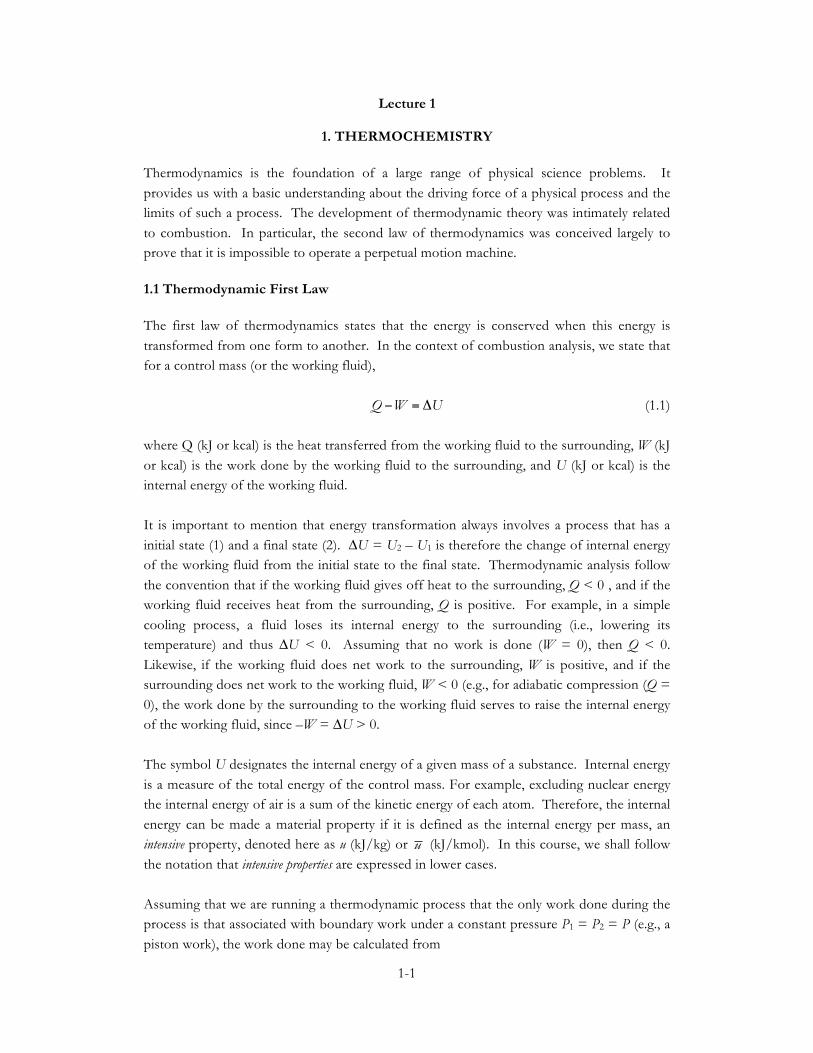
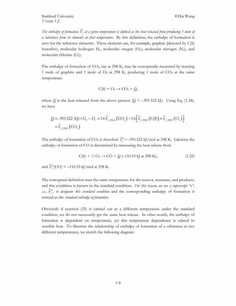
fh , to designate this standard condition and the corresponding enthalpy of formation is termed as the standard enthalpy of formation. Obviously if reaction (25) is carried out at a different temperature under the standard condition, we do not necessarily get the same heat release. In other words, the enthalpy of formation is dependent on temperature, yet this temperature dependence is related to sensible heat. To illustrate the relationship of enthalpy of formation of a substance at two different temperatures, we sketch the following diagram:


1-9

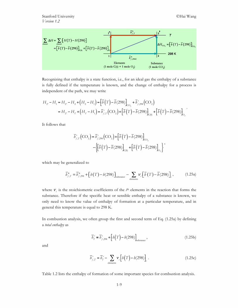
Recognizing that enthalpy is a state function, i.e., for an ideal gas the enthalpy of a substance is fully defined if the temperature is known, and the change of enthalpy for a process is independent of the path, we may write

H2' −H1 =H2' −H2 + H2 −H1( ) = h T( )− h (298)"#

$%CO2

+ h f ,298 CO2( )

=H2' −H1' + H1' −H1( ) = h f ,T CO2( )+ h T( )− h (298)"#

$%C(S)

+ h T( )− h (298)"#

$%O2

.

It follows that

h f ,T CO2( ) = h f ,298 CO2( )+ h T( )− h (298)"

#$%CO2

− h T( )− h (298)"#

$%C(S)

+ h T( )− h (298)"#

$%O2{ }

,

which may be generalized to ( ) ( )ν ⎡ ⎤= + − − −⎡ ⎤⎣ ⎦ ⎣ ⎦∑o o

, ,298 substanceelements

(298) (298)f T f i ih h h T h h T h , (1.25a)

where ν i is the stoichiometric coefficients of the ith elements in the reaction that forms the substance. Therefore if the specific heat or sensible enthalpy of a substance is known, we only need to know the value of enthalpy of formation at a particular temperature, and in general this temperature is equal to 298 K. In combustion analysis, we often group the first and second term of Eq. (1.25a) by defining a total enthalpy as

hT ≡ h f ,298

+ h T( )− h(298)#$

%&substance

, (1.25b)

and

h f ,T = hT

− ν i h T( )− h(298)"#

$%i

elements

∑ . (1.25c)

Table 1.2 lists the enthalpy of formation of some important species for combustion analysis.

Elements(1 mole C(s) + 1 mole O2)

Substance(1 mole CO2)

298 K

T

o,298f Kh

o,f Th

( ) ( )

( ) ( ) ( ) ( )

Δ = −⎡ ⎤⎣ ⎦

⎡ ⎤ ⎡ ⎤= − + −⎣ ⎦ ⎣ ⎦

∑ ∑

2C(S) O

298

298 298elements elements

H H T H

h T h h T h( ) ( )⎡ ⎤Δ = −⎣ ⎦2 2

CO CO298H h T h

1

1’ 2’

2

Elements(1 mole C(s) + 1 mole O2)

Substance(1 mole CO2)

298 K

T

o,298f Kh

o,f Th

( ) ( )

( ) ( ) ( ) ( )

Δ = −⎡ ⎤⎣ ⎦

⎡ ⎤ ⎡ ⎤= − + −⎣ ⎦ ⎣ ⎦

∑ ∑

2C(S) O

298

298 298elements elements

H H T H

h T h h T h( ) ( )⎡ ⎤Δ = −⎣ ⎦2 2

CO CO298H h T h

1

1’ 2’

2


1-10

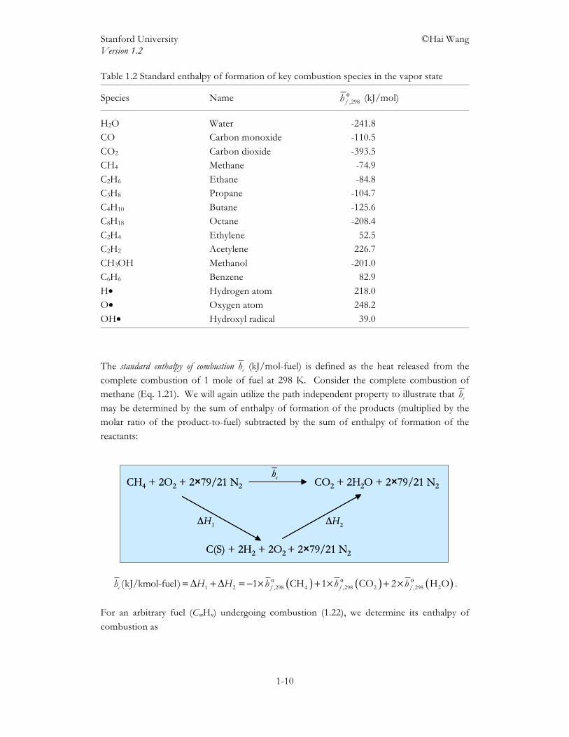
Table 1.2 Standard enthalpy of formation of key combustion species in the vapor state

Species Name o,298fh (kJ/mol)

H2O Water -241.8 CO Carbon monoxide -110.5 CO2 Carbon dioxide -393.5 CH4 Methane -74.9 C2H6 Ethane -84.8 C3H8 Propane -104.7 C4H10 Butane -125.6 C8H18 Octane -208.4 C2H4 Ethylene 52.5 C2H2 Acetylene 226.7 CH3OH Methanol -201.0 C6H6 Benzene 82.9 H• Hydrogen atom 218.0 O• Oxygen atom 248.2 OH• Hydroxyl radical 39.0

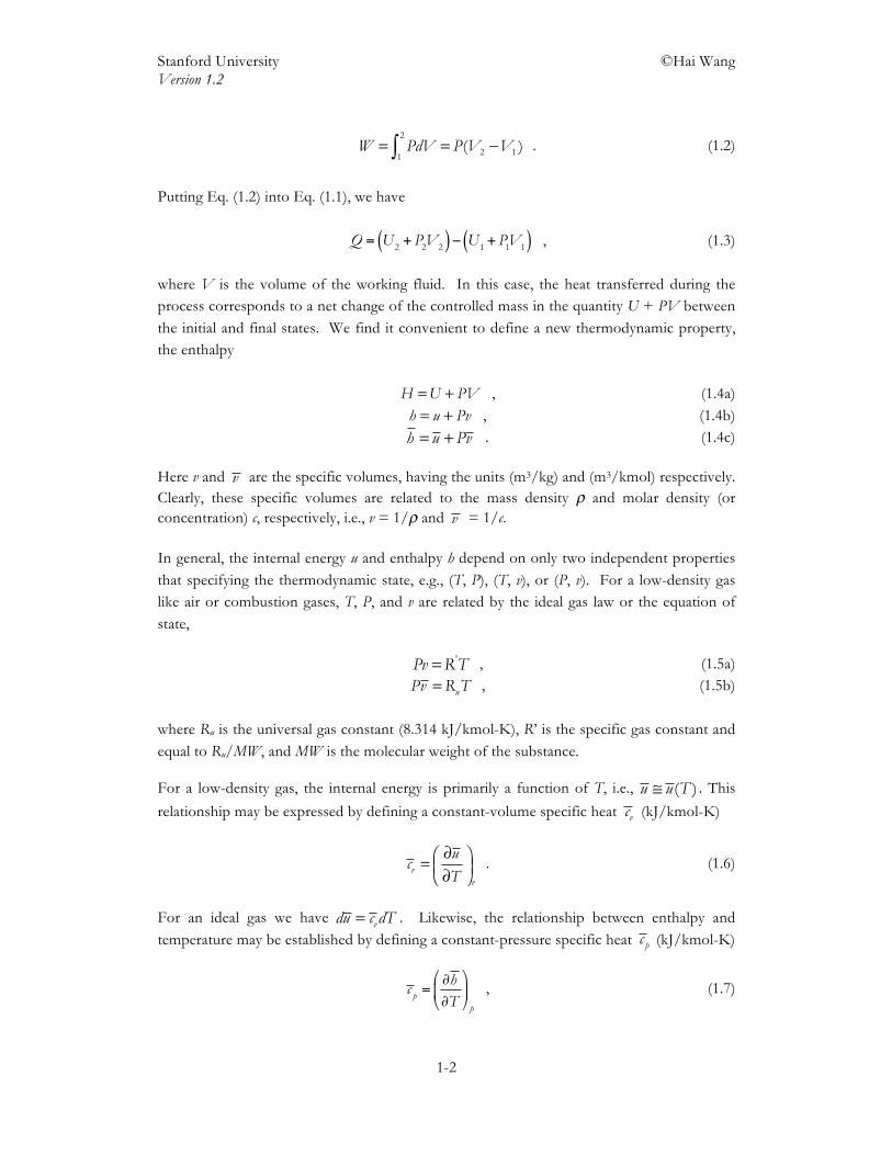
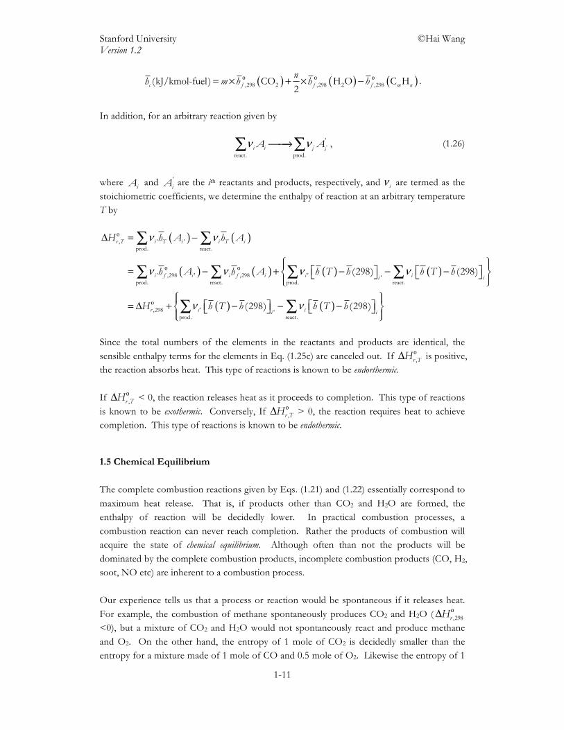
The standard enthalpy of combustion ch (kJ/mol-fuel) is defined as the heat released from the complete combustion of 1 mole of fuel at 298 K. Consider the complete combustion of methane (Eq. 1.21). We will again utilize the path independent property to illustrate that chmay be determined by the sum of enthalpy of formation of the products (multiplied by the molar ratio of the product-to-fuel) subtracted by the sum of enthalpy of formation of the reactants:

( ) ( ) ( )= Δ + Δ = − × + × + ×o o o1 2 ,298 4 ,298 2 ,298 2(kJ/kmol-fuel ) 1 CH 1 CO 2 H Oc f f fh H H h h h .

For an arbitrary fuel (CmHn) undergoing combustion (1.22), we determine its enthalpy of combustion as

CH4 + 2O2 + 2×79/21 N2 CO2 + 2H2O + 2×79/21 N2ch

Δ 1H

C(S) + 2H2 + 2O2 + 2×79/21 N2

Δ 2H

CH4 + 2O2 + 2×79/21 N2 CO2 + 2H2O + 2×79/21 N2ch

Δ 1H

C(S) + 2H2 + 2O2 + 2×79/21 N2

Δ 2H


1-11

( ) ( ) ( )= × + × −o o o,298 2 ,298 2 ,298(kJ/kmol-fuel ) CO H O C H

2c f f f m n

nh m h h h .

In addition, for an arbitrary reaction given by ν ν⎯⎯→∑ ∑ ' '

'

react. prod.i i i iA A , (1.26)

where iA and '

iA are the ith reactants and products, respectively, and ν i are termed as the stoichiometric coefficients, we determine the enthalpy of reaction at an arbitrary temperature T by

( ) ( )

( ) ( ) ( ) ( )

( ) ( )

ν ν

ν ν ν ν

ν ν

Δ = −

⎧ ⎫⎪ ⎪⎡ ⎤ ⎡ ⎤= − + − − −⎨ ⎬⎣ ⎦ ⎣ ⎦⎪ ⎪⎩ ⎭⎧ ⎫⎪ ⎪⎡ ⎤ ⎡ ⎤= Δ + − − −⎨ ⎬⎣ ⎦ ⎣ ⎦⎪⎩ ⎭

∑ ∑

∑ ∑ ∑ ∑

∑ ∑

o

o o

o

, ' 'prod. react.

' ,298 ' ,298 ' 'prod. react. prod. react.

,298 ' 'prod. react.

(298) (298)

(298) (298)

r T i T i i T i

i f i i f i i ii i

r i ii i

H h A h A

h A h A h T h h T h

H h T h h T h⎪

Since the total numbers of the elements in the reactants and products are identical, the sensible enthalpy terms for the elements in Eq. (1.25c) are canceled out. If Δ o

,r TH is positive, the reaction absorbs heat. This type of reactions is known to be endorthermic. If Δ o

,r TH < 0, the reaction releases heat as it proceeds to completion. This type of reactions is known to be exothermic. Conversely, If Δ o

,r TH > 0, the reaction requires heat to achieve completion. This type of reactions is known to be endothermic. 1.5 Chemical Equilibrium The complete combustion reactions given by Eqs. (1.21) and (1.22) essentially correspond to maximum heat release. That is, if products other than CO2 and H2O are formed, the enthalpy of reaction will be decidedly lower. In practical combustion processes, a combustion reaction can never reach completion. Rather the products of combustion will acquire the state of chemical equilibrium. Although often than not the products will be dominated by the complete combustion products, incomplete combustion products (CO, H2, soot, NO etc) are inherent to a combustion process. Our experience tells us that a process or reaction would be spontaneous if it releases heat. For example, the combustion of methane spontaneously produces CO2 and H2O (Δ o

,298rH<0), but a mixture of CO2 and H2O would not spontaneously react and produce methane and O2. On the other hand, the entropy of 1 mole of CO2 is decidedly smaller than the entropy for a mixture made of 1 mole of CO and 0.5 mole of O2. Likewise the entropy of 1


1-12

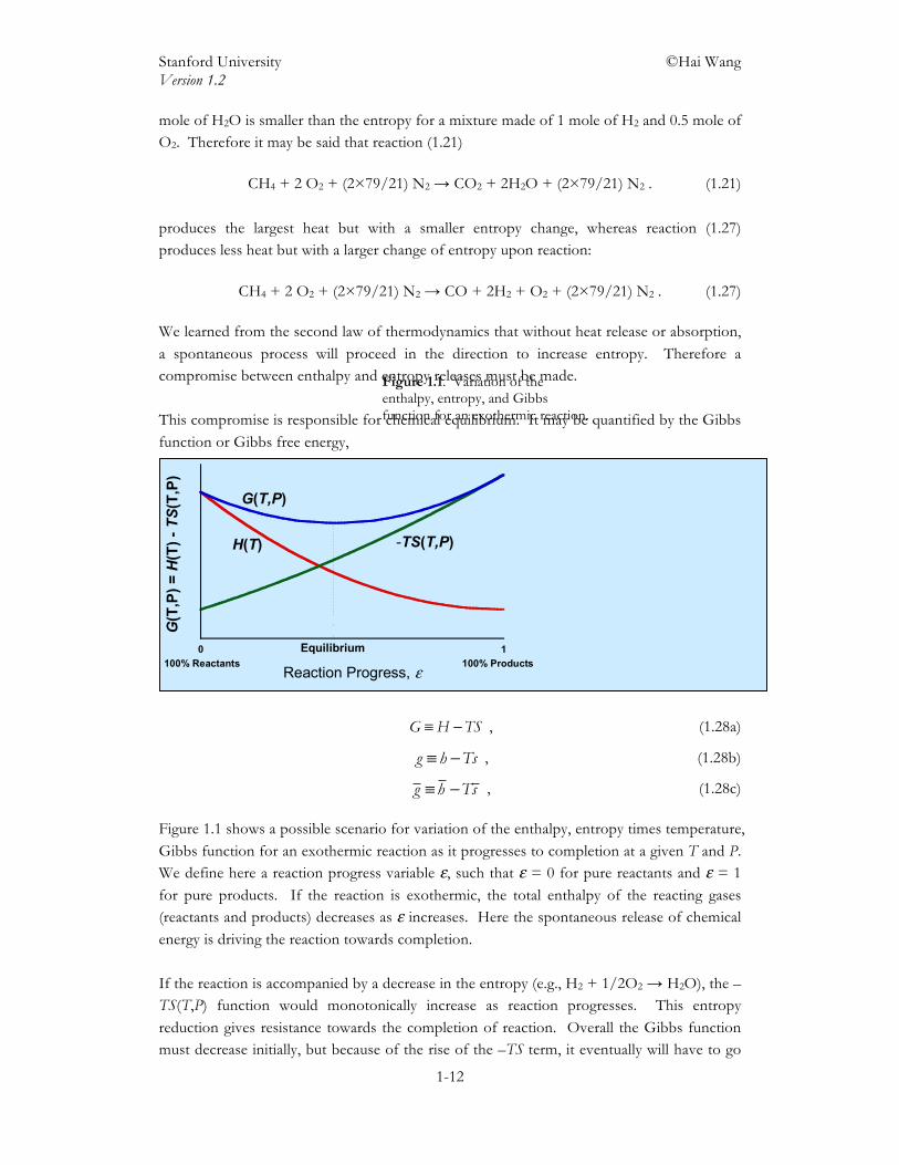
mole of H2O is smaller than the entropy for a mixture made of 1 mole of H2 and 0.5 mole of O2. Therefore it may be said that reaction (1.21) CH4 + 2 O2 + (2×79/21) N2 → CO2 + 2H2O + (2×79/21) N2 . (1.21) produces the largest heat but with a smaller entropy change, whereas reaction (1.27) produces less heat but with a larger change of entropy upon reaction: CH4 + 2 O2 + (2×79/21) N2 → CO + 2H2 + O2 + (2×79/21) N2 . (1.27) We learned from the second law of thermodynamics that without heat release or absorption, a spontaneous process will proceed in the direction to increase entropy. Therefore a compromise between enthalpy and entropy releases must be made. This compromise is responsible for chemical equilibrium. It may be quantified by the Gibbs function or Gibbs free energy,

≡ −G H TS , (1.28a)

≡ −g h Ts , (1.28b)

≡ −g h Ts , (1.28c) Figure 1.1 shows a possible scenario for variation of the enthalpy, entropy times temperature, Gibbs function for an exothermic reaction as it progresses to completion at a given T and P. We define here a reaction progress variable ε, such that ε = 0 for pure reactants and ε = 1 for pure products. If the reaction is exothermic, the total enthalpy of the reacting gases (reactants and products) decreases as ε increases. Here the spontaneous release of chemical energy is driving the reaction towards completion. If the reaction is accompanied by a decrease in the entropy (e.g., H2 + 1/2O2 → H2O), the –TS(T,P) function would monotonically increase as reaction progresses. This entropy reduction gives resistance towards the completion of reaction. Overall the Gibbs function must decrease initially, but because of the rise of the –TS term, it eventually will have to go

0 1

G(T

,P) =

H(T

) - TS(

T,P)

Reaction Progress, ε100% Reactants 100% Products

H(T) -TS(T,P)

G(T,P)

Equilibrium

Figure 1.1. Variation of the enthalpy, entropy, and Gibbs function for an exothermic reaction.


1-13

up as ε increases. In other words, the Gibbs function must reach a minimum at some point. The definition of chemical equilibrium is therefore

( )ε

=,

0dG T P

d, (1.29a)

or simply ( ) =, 0dG T P . (1.29b) Again, the above equilibrium criterion represents a compromise of H and –ST, since both of them prefer to minimize themselves. Therefore, the driving force of chemical reaction lies in the minimization of the Gibbs function. Now let us consider an arbitrary reaction given by Eq. (1.26). The Gibbs function of the reacting gas may be written as ( ) ( ) ( )= +∑ ∑ ' '

react. prod.

, , ,i i i iG T P n g T P n g T P , (1.30)

where ni is the molar number of the ith species. Putting Eq. (1.30) into (1.29a), we obtain, for constant T and P,

( ) ( ) ( )ε ε ε

= + =∑ ∑ ''

react. prod.

,, , 0i i

i i

dG T P dn dng T P g T P

d d d, (1.31)

Conservation of mass requires that

( )γ εν ε ν ε ν ε ν ε ν ε ν ε

− = − = − = = = ='1 2 1' 2 '

1 2 1' 2 ' '

1 1 1 1 1 1... N N

n n

dn dndn dn dn dnd d d d d d

, (1.32)

where N and N’ are the total numbers of reactants and products, respectively, and ( )γ ε is a function that depends only on ε. Combining equations (1.31) and (1.32), we obtain

( ) ( ) ( )γ ε ν ν⎡ ⎤− + =⎢ ⎥⎣ ⎦∑ ∑ ' 'react. prod.

, , 0i i i ig T P g T P . (1.33)

Since ( )γ ε ≠ 0 , we see that equilibrium state is given by

( ) ( )ν ν− + =∑ ∑ ' '

react. prod.

, , 0i i i ig T P g T P . (1.34)

The function ig is the Gibbs function of species i, which may be expressed by


1-14

( ) ( ) ( ) ( ) ( )⎡ ⎤⎛ ⎞= − = − − ⎜ ⎟⎢ ⎥⎝ ⎠⎣ ⎦o o o

o, lni f i f i u

Pg T P h T Ts T h T T s T R

P. (1.35)

We now define a standard Gibbs function ( )=o o, 1 atmg T P as

( ) ( ) ( )= −o o o

f ig T h T Ts T , (1.36)

and re-write Eq. (1.35) as

( ) ( ) ⎛ ⎞= + ⎜ ⎟⎝ ⎠o

o, lni u

Pg T P g T R T

P. (1.37)

Putting Eq. (1.37) into (1.34) and rearranging, we have

( ) ( )ν ν ν ν⎡ ⎤⎛ ⎞ ⎛ ⎞− = − −⎢ ⎥⎜ ⎟ ⎜ ⎟⎝ ⎠ ⎝ ⎠⎣ ⎦

∑ ∑ ∑ ∑o oo o'

' ' 'prod. react. prod. react.

ln lni ii i i i u i i

P Pg T g T R T

P P, (1.38)

where Pi is the partial pressure of species i, and of course, oP = 1 atm. The left-hand side of the above equation may be defined as the standard Gibbs function change of reaction, ( ) ( ) ( )ν νΔ ≡ −∑ ∑o o o

' 'prod. react.

r i i i iG T g T g T (1.39) The right-hand side of Eq. (1.38) may be re-arranged to yield

( )ν

ν

⎛ ⎞⎜ ⎟Δ = − ⎜ ⎟⎜ ⎟⎝ ⎠

∏∏

o

''

prod.

react.

ln

i

i

i

r ui

P

G T R TP

. (1.40)

or

( ) ( )ν

ν

⎡ ⎤Δ≡ = −⎢ ⎥

⎣ ⎦

∏∏

o''

prod.

react.

exp

i

i

ir

pi u

PG T

K TP R T

. (1.41)

where Kp(T) is the equilibrium constant of the reaction. Note that by neglecting oP in Eqs. (1.40) and (1.41), we have forced Pi to take the unit of atm. The equilibrium constant may also be defined by the concentrations of the reactants and products,


1-15

( ) ( ) ( )( )' '' '

prod. prod.

react. react.

i i

i i

i i

c u p ui i

c P

K T R T K T R Tc P

ν ν

ν νν ν

−Δ −Δ≡ = =∏ ∏∏ ∏

, (1.42)

where νΔ = −∑ ∑'

prod. react.i iv v .

There are several important facts about the equilibrium constant. (a) While Kp is defined as the pressure ratio of the products and reactants (Eq. 1.41), this

equilibrium constant is a function of temperature only. (b) Consider the reaction H2O = H2 + ½ O2. (1.43f) The equilibrium constant for the forward direction of the reaction is

( ) = 2 2

2

1 2H O

,H O

p f

P PK T

P.

We may also write the reaction in the back direction, H2 + ½ O2 = H2O , (1.43b) and its equilibrium constant

( ) = 2

2 2

H O, 1 2

H Op b

PK T

P P.

Obviously,

( ) ( )=,

,

1p f

p b

K TK T

.

(c) Reaction (43f) may be written alternatively as 2H2O = 2H2 + O2, (1.43f’) with its equilibrium constant

( ) = 2 2

2

2H O'

, 2H O

p f

P PK T

P .


1-16

Comparing the equilibrium constants for the two forward reactions, we see that

( ) ( )⎡ ⎤= ⎣ ⎦2'

, ,p f p fK T K T .

(d) Consider the following two reactions H2 = 2 H•. (1.44f) H2O = H• + OH• (1.45f) (where the • denotes that the species is a free radical). We have

( ) •=2

2H

,44H

p f

PK T

P and ( ) • •=

2

H OH,45

H Op f

P PK T

P .

A linear combination of reactions (43f-45f) yield H2O = ½ H2 + OH• . (1.46f) A little algebra tells us that (e) While Kp is not a function of pressure, Kc generally is dependent on pressure so long as

νΔ ≠ 0 . On the other hand, if νΔ = 0 , Kc(T) = Kp(T). (f) The equilibrium constant of a given reaction may be determined if the enthalpy of

formation and the entropy of reactants and products are known through Eqs. (1.36), (1.39) and (1.41).

(g) The definition of Kp tells us that the reaction would be more complete if Kp is larger. A

larger Kp may be accomplished with a larger, negative ( )Δ orG T . Combining Eqs. (1.36)

and (39), we see that

( ) ( ) ( ) ( ) ( )

( ) ( )

ν ν ν ν⎡ ⎤ ⎡ ⎤

Δ ≡ − − −⎢ ⎥ ⎢ ⎥⎣ ⎦ ⎣ ⎦

= Δ − Δ

∑ ∑ ∑ ∑o o o o o

o o

' , ' , ' 'prod. react. prod. react.

r i f i i f i i i i i

r r

G T h T h T T s T s T

H T T S T

, (1.47)

where ( )Δ o

rS T is termed as the entropy of reaction. Therefore a large, negative

( )Δ orH T (reaction being highly exothermic) favors a large Kp , whereas a large, positive ( )Δ o

rS T (reaction creating a large amount of entropy) also favors a large Kp or promotes the completion of the reaction.


1-17

1.6 Adiabatic Flame Temperature With the concepts of chemical equilibrium understood, we may now try to calculate the equilibrium composition of a combustion reaction. In doing so, we wish to define the adiabatic flame temperature. Consider an adiabatic combustion process whereby the reactants enters into a combustor at temperature T0, and products exit the combustor at the adiabatic flame temperature Tad. Since the process is adiabatic (Q = 0 ), we have ( ) ( )− =prod. react. 0 0adH T H T . (1.48)

We now expand Eq. (1.48) using the total enthalpy equation for each species (Eq. 1.25b),

( ) ( )

( ) ( )

ν ν ν ν ν

ν

⎡ ⎤⎡ ⎤− = − + −⎢ ⎥ ⎣ ⎦

⎣ ⎦⎡ ⎤− − =⎣ ⎦

∑ ∑ ∑ ∑ ∑

∑

o o0' , ' , ' ,298, ' ,298, ' '

prod. react. prod. react. prod.

0react.

298

298 0

adi T i i T i i f i i f i i ad i

i i

h h h h h T h

h T h

.(1.49)

Obviously the first term on the right-hand side of Eq. (1.49) is the standard enthalpy of reaction Δ o

,298rH . The second term determines the sensible heat needed to heat the products from 298 K to the adiabatic flame temperature Tad. To simplify our analysis, we shall assume that the reactants enter into the reactor at T0 = 298 K so the third term becomes 0. Rearranging Eq. (1.49), we see that

( ) ( )ν ⎡ ⎤−Δ = −⎣ ⎦∑o,298 ' '

prod.

298r i ad iH h T h . (1.50)

In other words, the adiabatic flame temperature is obtained when all the heat released from a combustion reaction is used to raise the product temperature from 298 to Tad. The existence of chemical equilibrium makes the calculation of this adiabatic flame temperature a bit more involved. Specifically, while the values of ν i are always well defined, ν 'i is not since it is dependent on the equilibrium composition of the products.

Consider the combustion of 1 mole of carbon (graphite) in 1 mole of oxygen at a pressure of 1 atm. 1 mole C(S) + 1 mole O2 → x CO2 + yCO + zO2. (1.51) The reactant temperature is 298 K. The principle of chemical equilibrium states that the products cannot be entirely CO2. Rather, a small amount of CO (y moles) must be produced along with z moles of O2 unused. These products are in equilibrium at the adiabatic flame temperature among themselves through


1-18

CO2 = CO + ½ O2 , (1.52)

with its equilibrium constant given by

K p Tad( ) = PCOPO2

1 2

PCO2

=yz 1 2

xP

x + y + z

⎛⎝⎜

⎞⎠⎟

1 2

= exp −ΔGr0 RuTad( ) . (1.53)

(We need to recognize that the products of a combustion process cannot be in equilibrium with the reactants of the process. Rather it is the products that are in equilibrium among themselves.) Since there are four unknowns in Eq. (1.53) (i.e., x, y, z and Tad), we need to provide three more equations to solve this problem. Two of these equations come from mass conservation:

Carbon: + =1 molx y , (1.54) Oxygen: + + =2 2 2 molx y z . (1.55)

The last equation is given by Eq. (1.50), which may be expanded to give

( ) ( ) ( ) ( )

( ) ( ) ( ) ( )

⎡ ⎤ ⎡ ⎤− + = −⎣ ⎦⎣ ⎦

⎡ ⎤ ⎡ ⎤+ − + −⎣ ⎦ ⎣ ⎦

o o

2

2

,298 2 ,298 CO

CO O

CO CO 298

298 298

f f ad

ad ad

xh yh x h T h

y h T h z h T h.(1.56)

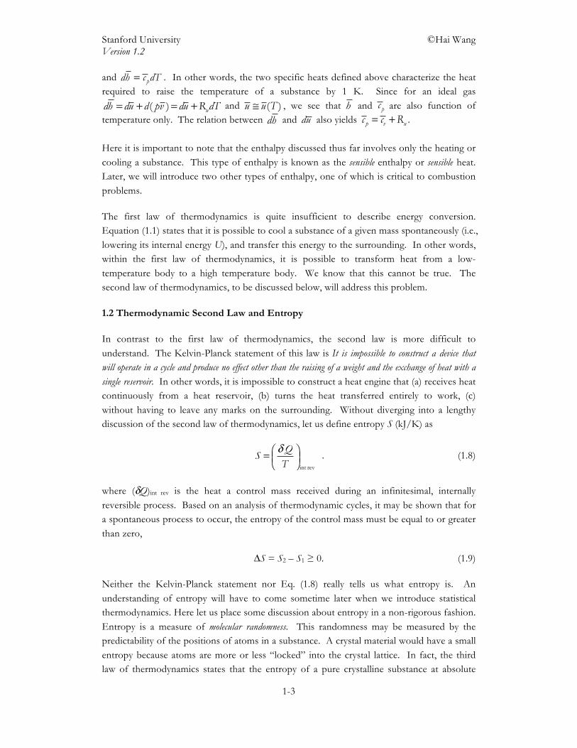
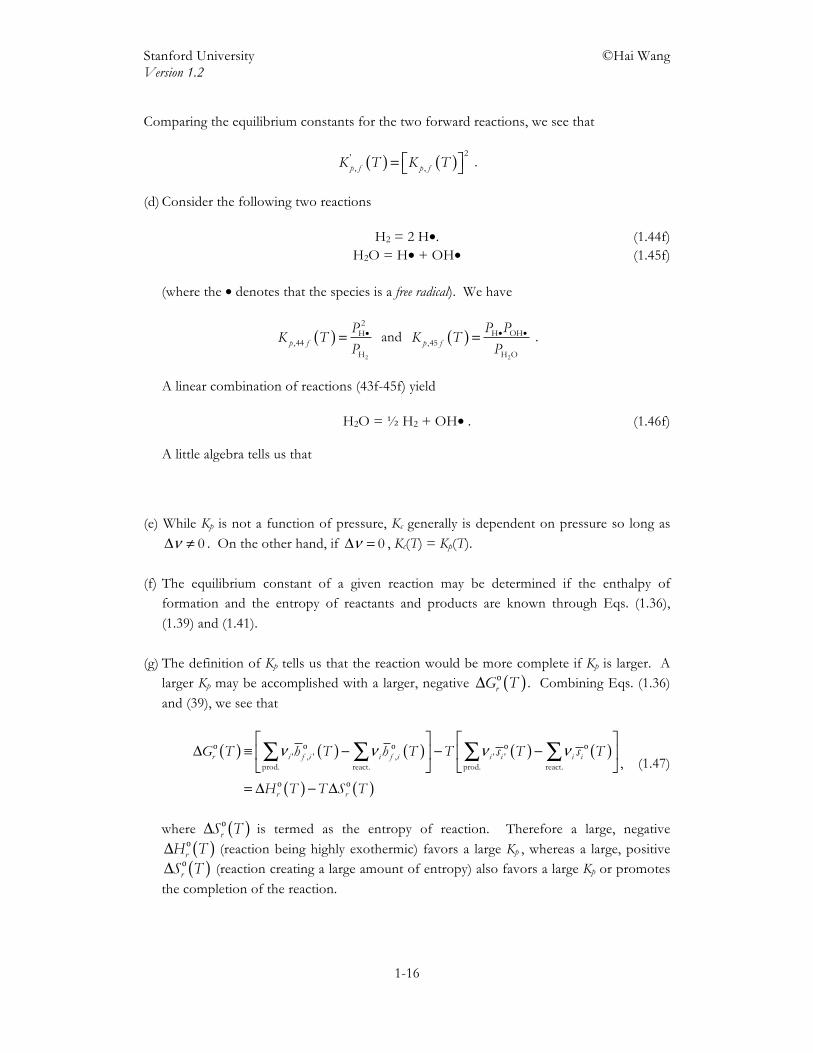
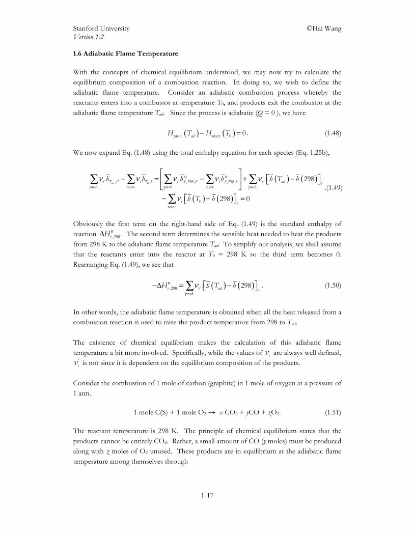
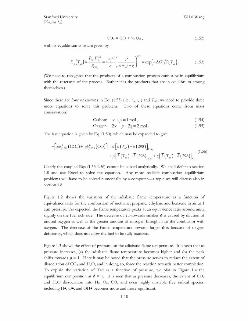
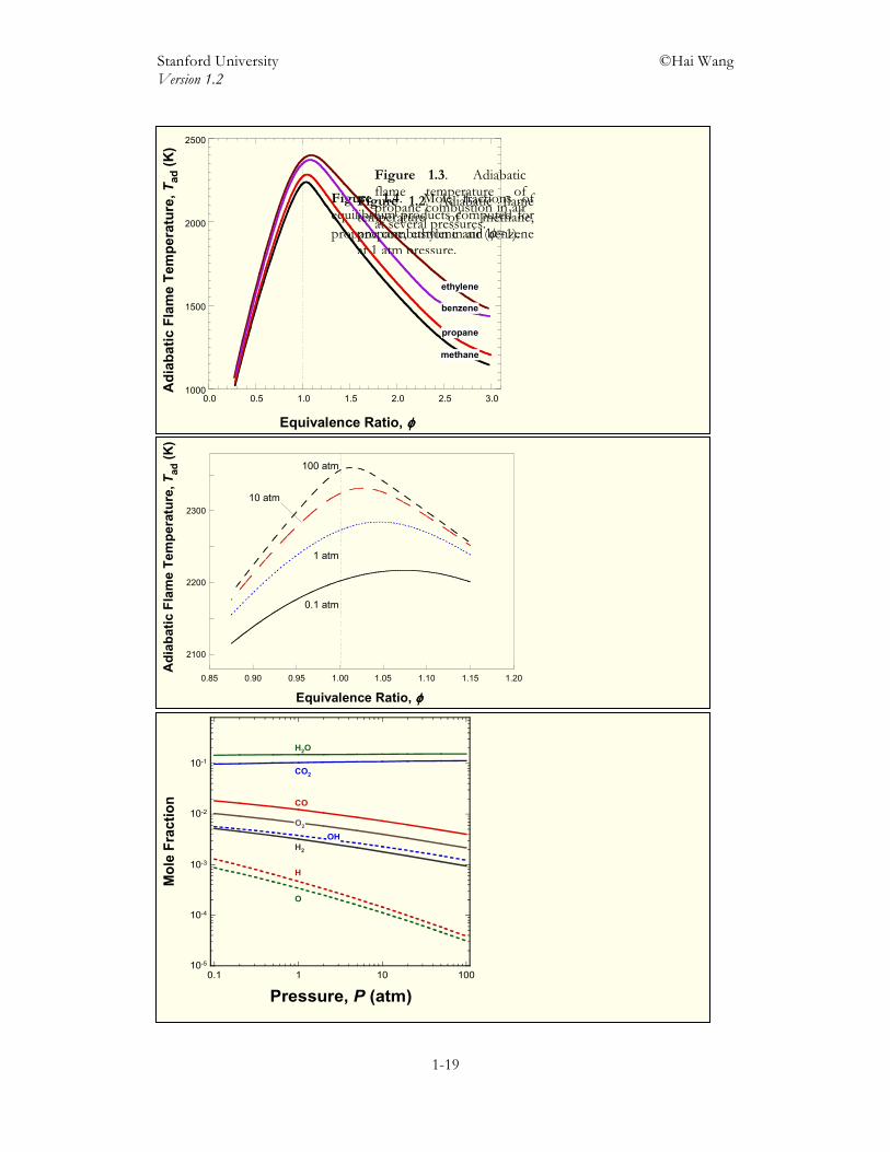
Clearly the coupled Eqs (1.53-1.56) cannot be solved analytically. We shall defer to section 1.8 and use Excel to solve the equation. Any more realistic combustion equilibrium problems will have to be solved numerically by a computer—a topic we will discuss also in section 1.8. Figure 1.2 shows the variation of the adiabatic flame temperature as a function of equivalence ratio for the combustion of methane, propane, ethylene and benzene in air at 1 atm pressure. As expected, the flame temperature peaks at an equivalence ratio around unity, slightly on the fuel rich side. The decrease of Tad towards smaller φ is caused by dilution of unused oxygen as well as the greater amount of nitrogen brought into the combustor with oxygen. The decrease of the flame temperature towards larger φ is because of oxygen deficiency, which does not allow the fuel to be fully oxidized. Figure 1.3 shows the effect of pressure on the adiabatic flame temperature. It is seen that as pressure increases, (a) the adiabatic flame temperature becomes higher and (b) the peak shifts towards φ = 1. Here it may be noted that the pressure serves to reduce the extent of dissociation of CO2 and H2O, and in doing so, force the reaction towards better completion. To explain the variation of Tad as a function of pressure, we plot in Figure 1.4 the equilibrium composition at φ = 1. It is seen that as pressure decreases, the extent of CO2 and H2O dissociation into H2, O2, CO, and even highly unstable free radical species, including H•, O•, and OH• becomes more and more significant.


1-19

2100

2200

2300

0.85 0.90 0.95 1.00 1.05 1.10 1.15 1.20

0.1 atm

1 atm

10 atm

100 atm

Adi

abat

ic F

lam

e Te

mpe

ratu

re, T

ad (K

)

Equivalence Ratio, φ

Figure 1.3. Adiabatic flame temperature of propane combustion in air at several pressures.

Figure 1.4. Mole fractions of equilibrium products computed for propane combustion in air (φ=1).

10-5

10-4

10-3

10-2

10-1

0.1 1 10 100

Mol

e Fr

actio

n

Pressure, P (atm)

H2O

CO2

CO

O2

OHH2

H

O

1000

1500

2000

2500

0.0 0.5 1.0 1.5 2.0 2.5 3.0

methane

ethylene

propane

benzene

Adi

abat

ic F

lam

e Te

mpe

ratu

re, T

ad (K

)

Equivalence Ratio, φ

Figure 1.2. Adiabatic flame temperature of methane, propane, ethylene and benzene at 1 atm pressure.


1-20

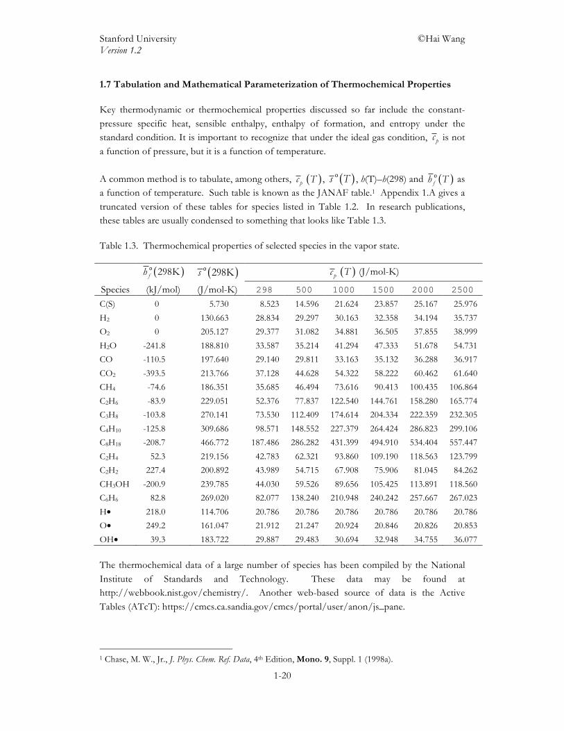
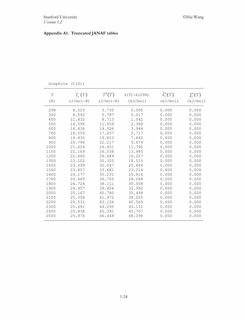
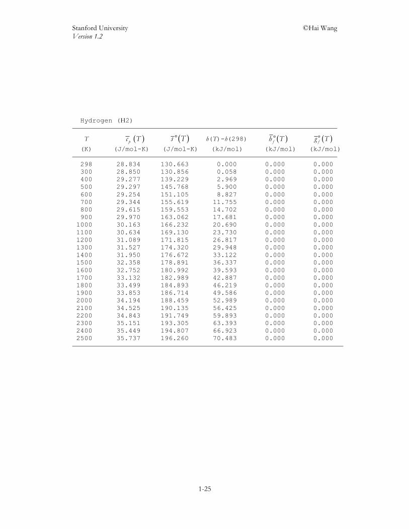
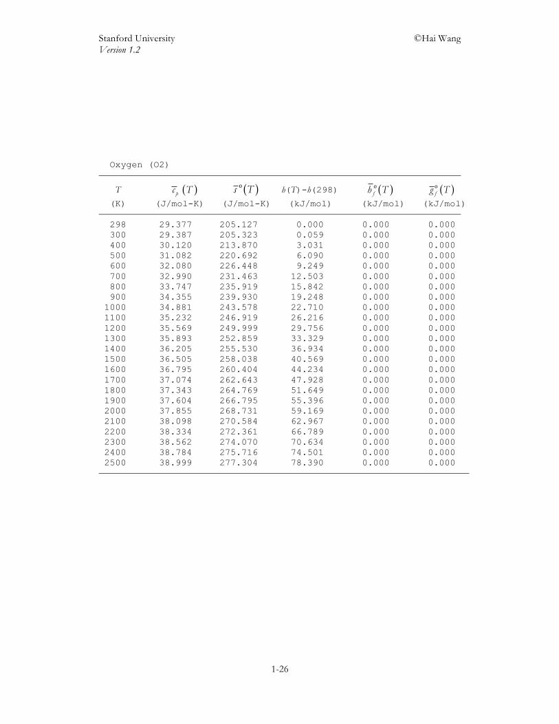
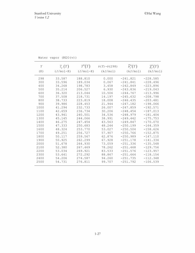
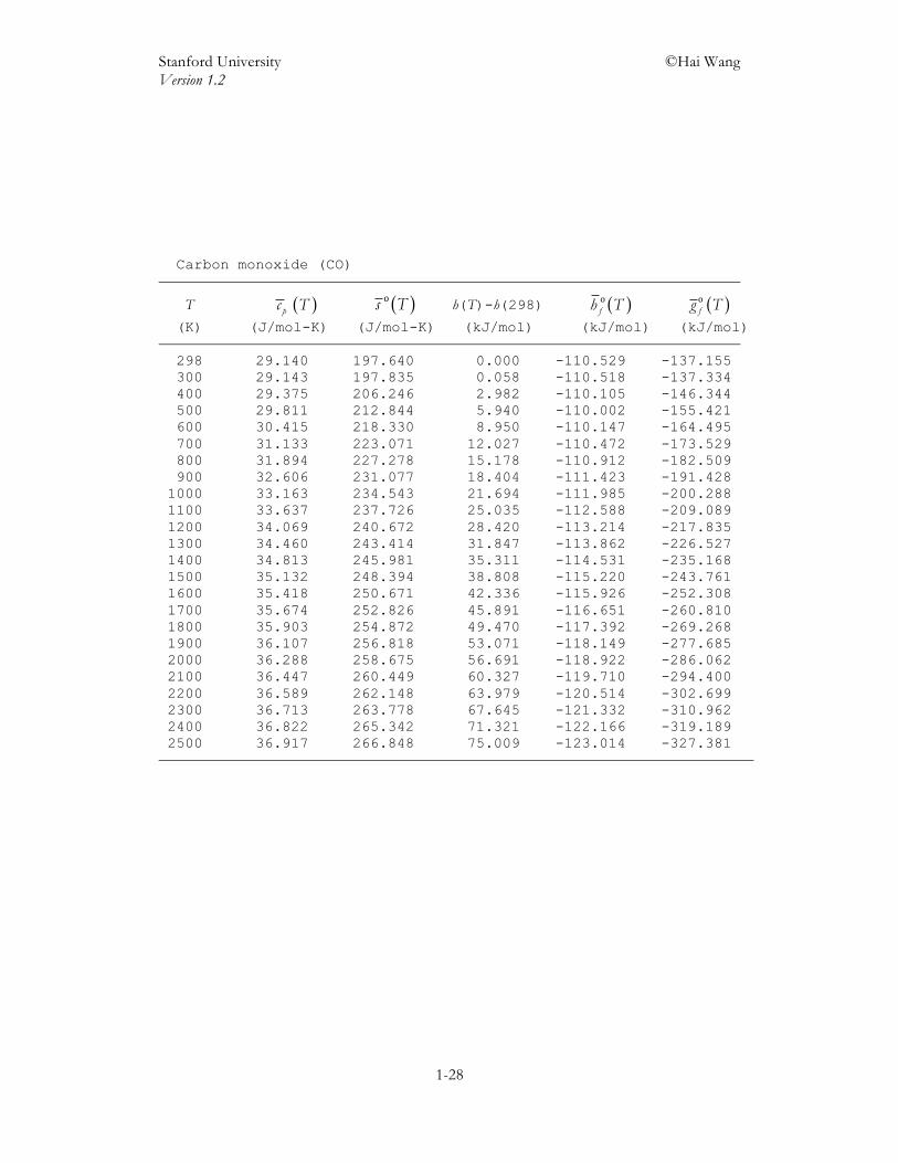
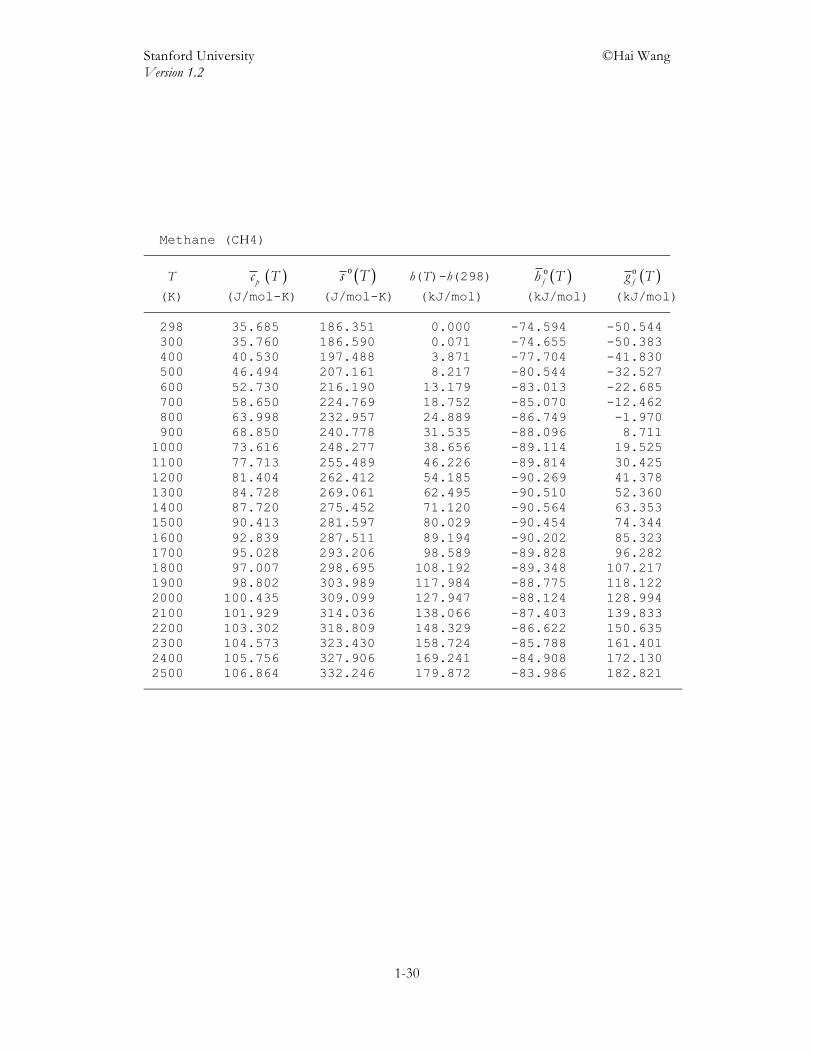
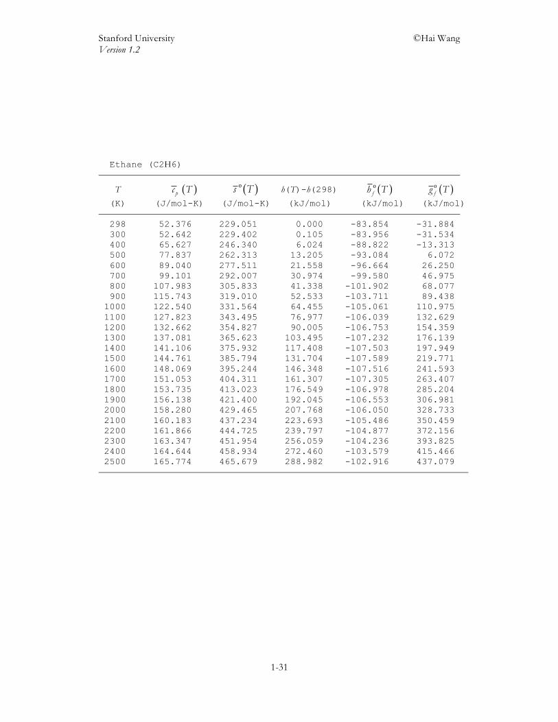
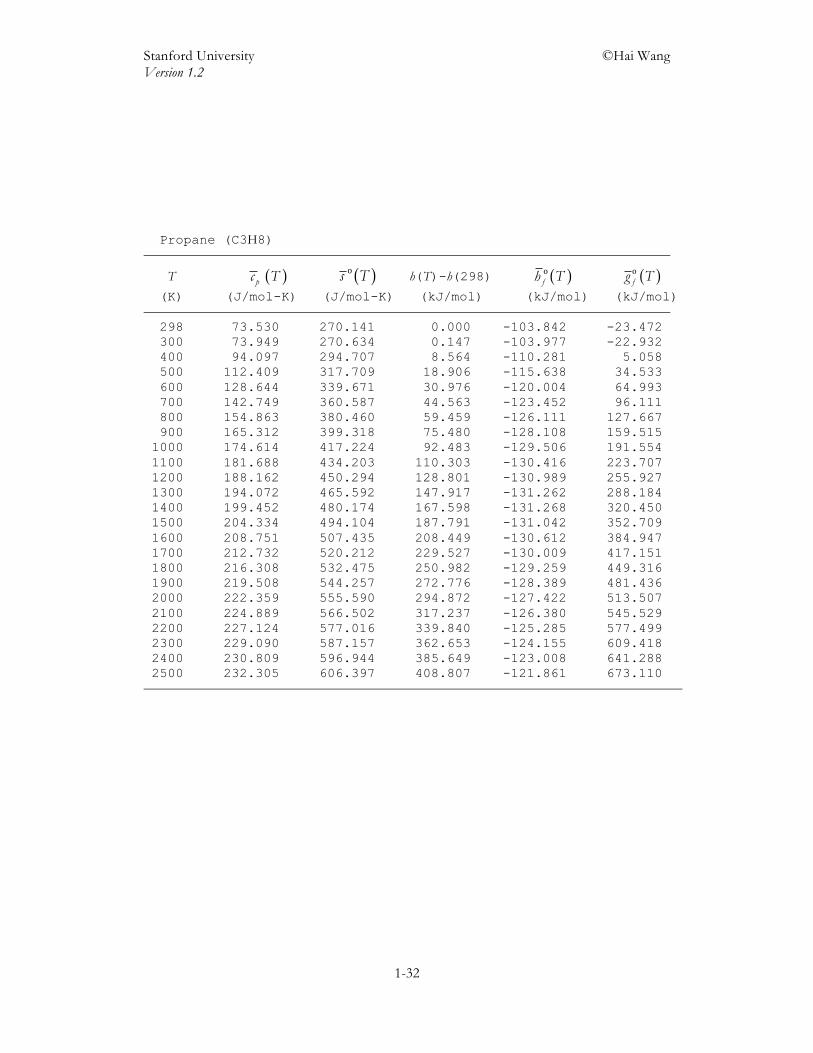
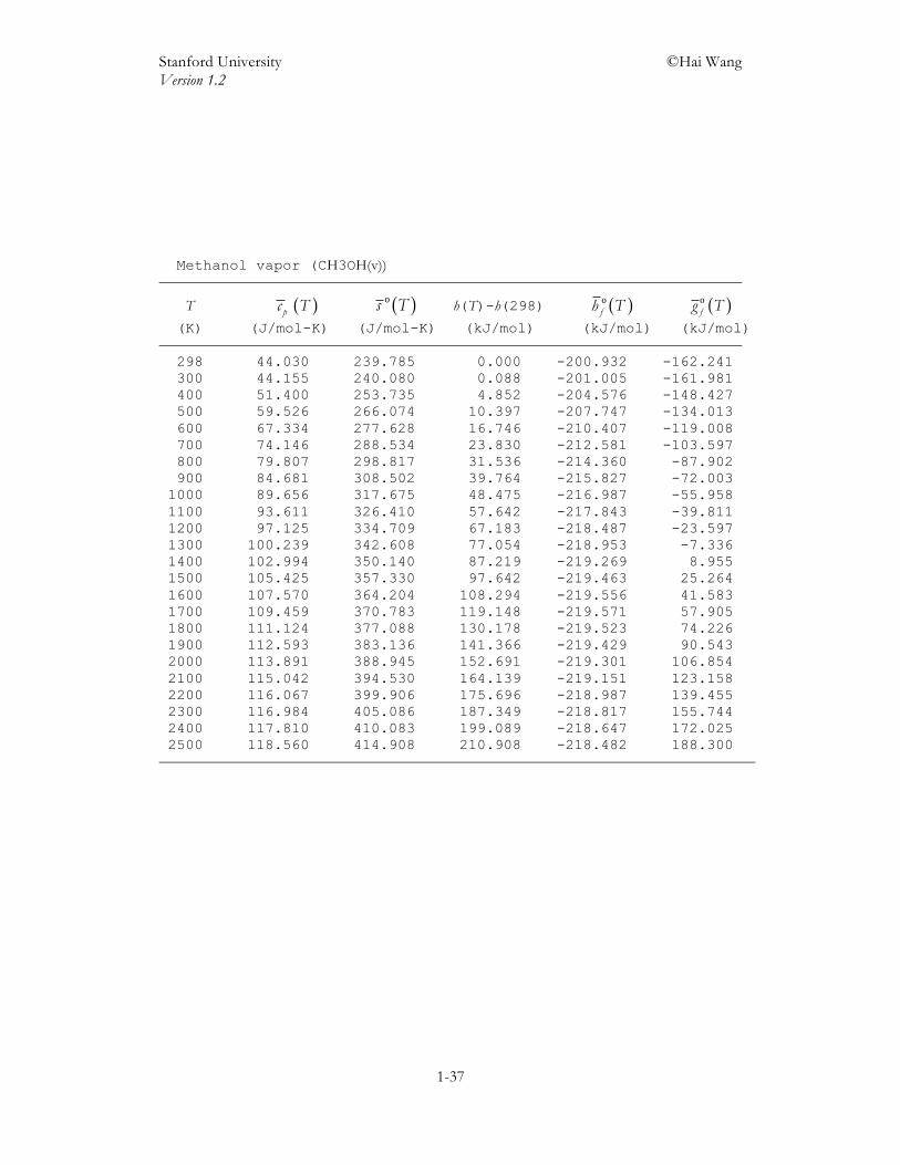
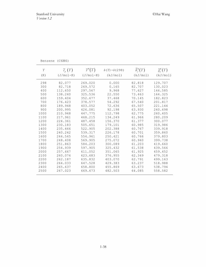
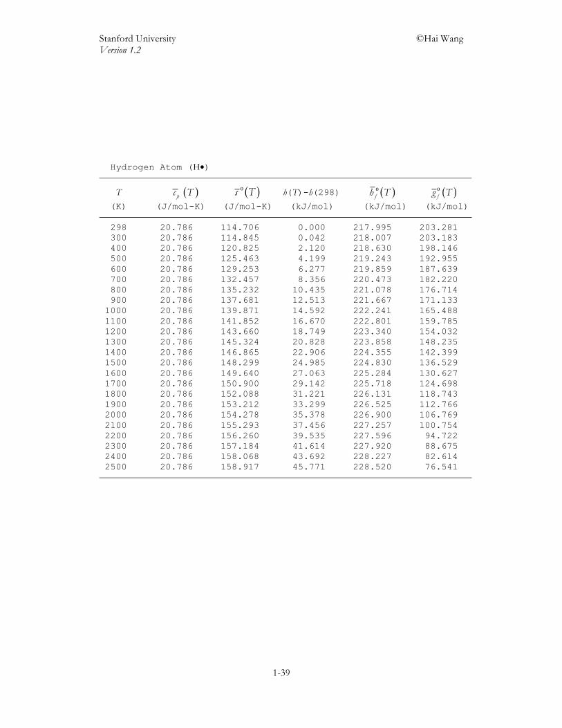
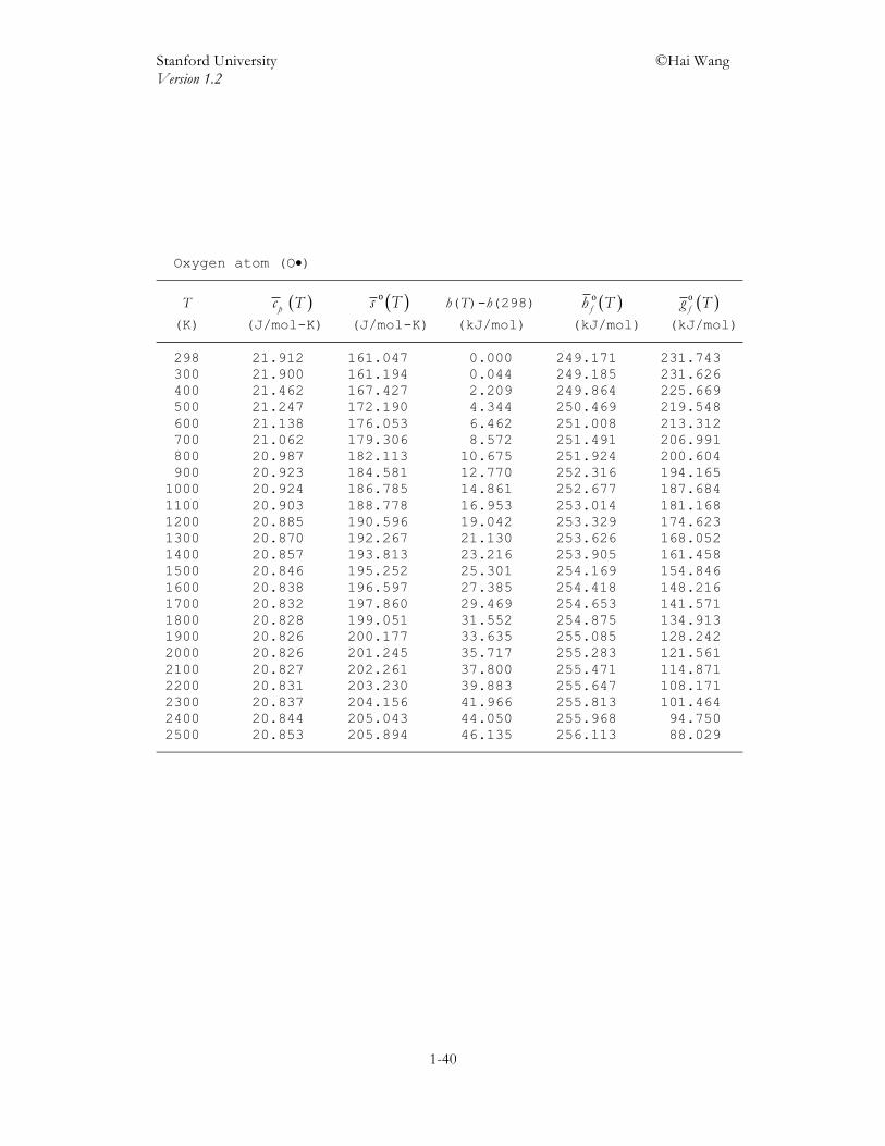
1.7 Tabulation and Mathematical Parameterization of Thermochemical Properties Key thermodynamic or thermochemical properties discussed so far include the constant-pressure specific heat, sensible enthalpy, enthalpy of formation, and entropy under the standard condition. It is important to recognize that under the ideal gas condition, pc is not a function of pressure, but it is a function of temperature. A common method is to tabulate, among others, ( )pc T , ( )os T , h(T)–h(298) and ( )o

fh T as a function of temperature. Such table is known as the JANAF table.1 Appendix 1.A gives a truncated version of these tables for species listed in Table 1.2. In research publications, these tables are usually condensed to something that looks like Table 1.3. Table 1.3. Thermochemical properties of selected species in the vapor state.

( )o 298Kfh ( )o 298Ks ( )pc T (J/mol-K)

Species (kJ/mol) (J/mol-K) 298 500 1000 1500 2000 2500

C(S) 0 5.730 8.523 14.596 21.624 23.857 25.167 25.976 H2 0 130.663 28.834 29.297 30.163 32.358 34.194 35.737 O2 0 205.127 29.377 31.082 34.881 36.505 37.855 38.999 H2O -241.8 188.810 33.587 35.214 41.294 47.333 51.678 54.731 CO -110.5 197.640 29.140 29.811 33.163 35.132 36.288 36.917 CO2 -393.5 213.766 37.128 44.628 54.322 58.222 60.462 61.640 CH4 -74.6 186.351 35.685 46.494 73.616 90.413 100.435 106.864

C2H6 -83.9 229.051 52.376 77.837 122.540 144.761 158.280 165.774

C3H8 -103.8 270.141 73.530 112.409 174.614 204.334 222.359 232.305

C4H10 -125.8 309.686 98.571 148.552 227.379 264.424 286.823 299.106

C8H18 -208.7 466.772 187.486 286.282 431.399 494.910 534.404 557.447

C2H4 52.3 219.156 42.783 62.321 93.860 109.190 118.563 123.799

C2H2 227.4 200.892 43.989 54.715 67.908 75.906 81.045 84.262 CH3OH -200.9 239.785 44.030 59.526 89.656 105.425 113.891 118.560

C6H6 82.8 269.020 82.077 138.240 210.948 240.242 257.667 267.023

H• 218.0 114.706 20.786 20.786 20.786 20.786 20.786 20.786

O• 249.2 161.047 21.912 21.247 20.924 20.846 20.826 20.853 OH• 39.3 183.722 29.887 29.483 30.694 32.948 34.755 36.077 The thermochemical data of a large number of species has been compiled by the National Institute of Standards and Technology. These data may be found at http://webbook.nist.gov/chemistry/. Another web-based source of data is the Active Tables (ATcT): https://cmcs.ca.sandia.gov/cmcs/portal/user/anon/js_pane.

1 Chase, M. W., Jr., J. Phys. Chem. Ref. Data, 4th Edition, Mono. 9, Suppl. 1 (1998a).


1-21

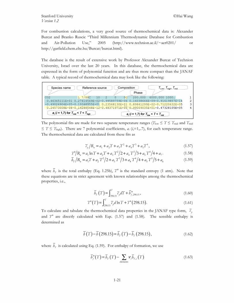
For combustion calculations, a very good source of thermochemical data is: Alexander Burcat and Branko Ruscic “Third Millennium Thermodynamic Database for Combustion and Air-Pollution Use,” 2005 (http://www.technion.ac.il/~aer0201/ or http://garfield.chem.elte.hu/Burcat/burcat.html). The database is the result of extensive work by Professor Alexander Burcat of Technion University, Israel over the last 20 years. In this database, the thermochemical data are expressed in the form of polynomial function and are thus more compact than the JANAF table. A typical record of thermochemical data may look like the following:

The polynomial fits are made for two separate temperature ranges (Tlow ≤ T ≤ Tmid and Tmid ≤ T ≤ Thigh). There are 7 polynomial coefficients, ai (i,=1,..7), for each temperature range. The thermochemical data are calculated from these fits as = + + + +2 3 4

1 2 3 4 5p uc R a a T a T a T a T , (1.57)

= + + + + +o 2 3 41 2 3 4 5 7ln 2 3 4us R a T a T a T a T a T a . (1.58)

= + + + + +2 3 4 51 2 3 4 5 62 3 4 5T uh R a T a T a T a T a T a (1.59)

where Th is the total enthalpy (Eq. 1.25b), os is the standard entropy (1 atm). Note that these equations are in strict agreement with known relationships among the thermochemical properties, i.e.,

( ) = +∫ o,298.15298.15

T

T p fh T c dT h , (1.60)

( ) ( )= +∫o o

298.15ln 298.15

T

ps T c d T s . (1.61)

To calculate and tabulate the thermochemical data properties in the JANAF type form, pc and os are directly calculated with Eqs. (1.57) and (1.58). The sensible enthalpy is determined as ( ) ( ) ( ) ( )− = −298.15 298.15T Th T h h T h , (1.62) where Th is calculated using Eq. (1.59). For enthalpy of formation, we use ( ) ( ) ( )ν= − ∑o

,elements

f T i T ih T h T h T (1.63)

CO2 L 7/88C 1O 2 0 0G 200.000 6000.000 1000. 1 0.46365111E+01 0.27414569E-02-0.99589759E-06 0.16038666E-09-0.91619857E-14 2 -0.49024904E+05-0.19348955E+01 0.23568130E+01 0.89841299E-02-0.71220632E-05 3 0.24573008E-08-0.14288548E-12-0.48371971E+05 0.99009035E+01-0.47328105E+05 4

Species name Reference sourcePhase

Composition TLow, Thigh, Tmid

ai (i = 1,7) for Tmid < T < Thigh ai (i = 1,7) for Tlow < T < Tmid

CO2 L 7/88C 1O 2 0 0G 200.000 6000.000 1000. 1 0.46365111E+01 0.27414569E-02-0.99589759E-06 0.16038666E-09-0.91619857E-14 2 -0.49024904E+05-0.19348955E+01 0.23568130E+01 0.89841299E-02-0.71220632E-05 3 0.24573008E-08-0.14288548E-12-0.48371971E+05 0.99009035E+01-0.47328105E+05 4

Species name Reference sourcePhase

Composition TLow, Thigh, Tmid

ai (i = 1,7) for Tmid < T < Thigh ai (i = 1,7) for Tlow < T < Tmid


1-22

where ν i represents the molecular composition of the substance. For example, a CxHyOz

species has ν =C x , ν =2H

2y and ν =2

2O z .

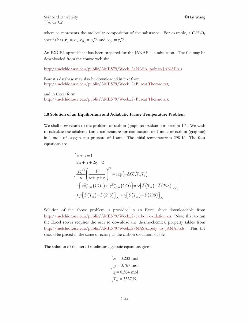
An EXCEL spreadsheet has been prepared for the JANAF like tabulation. The file may be downloaded from the course web site http://melchior.usc.edu/public/AME579/Week_2/NASA_poly to JANAF.xls. Burcat’s database may also be downloaded in text form http://melchior.usc.edu/public/AME579/Week_2/Burcat Thermo.txt, and in Excel form http://melchior.usc.edu/public/AME579/Week_2/Burcat Thermo.xls. 1.8 Solution of an Equilibrium and Adiabatic Flame Temperature Problem We shall now return to the problem of carbon (graphite) oxidation in section 1.6. We wish to calculate the adiabatic flame temperature for combustion of 1 mole of carbon (graphite) in 1 mole of oxygen at a pressure of 1 atm. The initial temperature is 298 K. The four equations are

( )

( ) ( ) ( ) ( )

( ) ( ) ( ) ( )

+ =⎧⎪ + + =⎪⎪ ⎛ ⎞⎪ = −Δ⎜ ⎟⎨ + +⎝ ⎠⎪

⎡ ⎤⎪ ⎡ ⎤− + = −⎣ ⎦⎣ ⎦⎪⎪ ⎡ ⎤ ⎡ ⎤+ − + −⎣ ⎦ ⎣ ⎦⎩

o o

2

2

1 21 20

,298 2 ,298 CO

CO O

1

2 2 2

exp

CO CO 298

298 298

r u d

f f ad

ad ad

x y

x y z

yz PG R T

x x y z

xh yh x h T h

y h T h z h T h

.

Solution of the above problem is provided in an Excel sheet downloadable from http://melchior.usc.edu/public/AME579/Week_2/carbon oxidation.xls. Note that to run the Excel solver requires the user to download the thermochemical property tables from http://melchior.usc.edu/public/AME579/Week_2/NASA_poly to JANAF.xls. This file should be placed in the same directory as the carbon oxidation.xls file. The solution of this set of nonlinear algebraic equations gives

=⎧⎪ =⎪⎨ =⎪⎪ =⎩

0.233 mol

0.767 mol

0.384 mol

3537 Kad

x

y

z

T


1-23

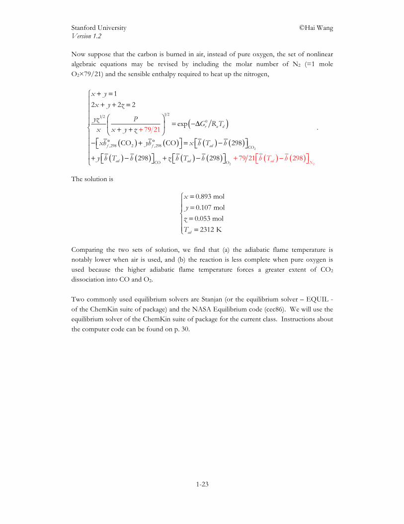
Now suppose that the carbon is burned in air, instead of pure oxygen, the set of nonlinear algebraic equations may be revised by including the molar number of N2 (=1 mole O2×79/21) and the sensible enthalpy required to heat up the nitrogen,

( )

( ) ( ) ( ) ( )

( ) ( ) ( ) ( ) ( ) ( )

+ =⎧⎪ + + =⎪⎪ ⎛ ⎞⎪ = −Δ⎜ ⎟⎨ + +⎝ ⎠⎪

⎡ ⎤⎪ ⎡ ⎤− + = −⎣ ⎦⎣ ⎦⎪⎪ ⎡ ⎤ ⎡ ⎤+ − +

+

⎡ ⎤−⎣ ⎦ ⎦ + ⎦⎣ ⎣⎩ −

o o

2

2 2

1 21 20

,298 2 ,298 CO

CO O

1

2 2 2

exp

CO CO

79 2

298

298 2

1

79 21 29898

r u d

f f a

d N

d

a aad d

x y

x y z

yz PG R T

x x y z

xh yh x h T h

y h T h z hh T h h T

.

The solution is

=⎧⎪ =⎪⎨ =⎪⎪ =⎩

0.893 mol

0.107 mol

0.053 mol

2312 Kad

x

y

z

T

Comparing the two sets of solution, we find that (a) the adiabatic flame temperature is notably lower when air is used, and (b) the reaction is less complete when pure oxygen is used because the higher adiabatic flame temperature forces a greater extent of CO2 dissociation into CO and O2. Two commonly used equilibrium solvers are Stanjan (or the equilibrium solver – EQUIL - of the ChemKin suite of package) and the NASA Equilibrium code (cec86). We will use the equilibrium solver of the ChemKin suite of package for the current class. Instructions about the computer code can be found on p. 30.


1-24

Appendix A1. Truncated JANAF tables Graphite (C(S))

T ( )pc T ( )os T h(T)-h(298) ( )ofh T ( )o

fg T

(K) (J/mol-K) (J/mol-K) (kJ/mol) (kJ/mol) (kJ/mol) 298 8.523 5.730 0.000 0.000 0.000 300 8.592 5.787 0.017 0.000 0.000 400 11.832 8.713 1.042 0.000 0.000 500 14.596 11.659 2.368 0.000 0.000 600 16.836 14.526 3.944 0.000 0.000 700 18.559 17.257 5.717 0.000 0.000 800 19.835 19.823 7.640 0.000 0.000 900 20.794 22.217 9.674 0.000 0.000 1000 21.624 24.451 11.795 0.000 0.000 1100 22.169 26.538 13.985 0.000 0.000 1200 22.660 28.489 16.227 0.000 0.000 1300 23.102 30.320 18.515 0.000 0.000 1400 23.499 32.047 20.846 0.000 0.000 1500 23.857 33.681 23.214 0.000 0.000 1600 24.177 35.231 25.616 0.000 0.000 1700 24.465 36.705 28.048 0.000 0.000 1800 24.724 38.111 30.508 0.000 0.000 1900 24.957 39.454 32.992 0.000 0.000 2000 25.167 40.740 35.498 0.000 0.000 2100 25.358 41.972 38.025 0.000 0.000 2200 25.531 43.156 40.569 0.000 0.000 2300 25.691 44.295 43.131 0.000 0.000 2400 25.838 45.391 45.707 0.000 0.000 2500 25.976 46.449 48.298 0.000 0.000


1-25

Hydrogen (H2)


fg T



1-26

Oxygen (O2)


fg T



1-27

Water vapor (H2O(v))


fg T

(K) (J/mol-K) (J/mol-K) (kJ/mol) (kJ/mol) (kJ/mol) 298 33.587 188.810 0.000 -241.821 -228.585 300 33.596 189.034 0.067 -241.841 -228.496 400 34.268 198.783 3.458 -242.849 -223.896 500 35.214 206.527 6.930 -243.836 -219.043 600 36.320 213.044 10.506 -244.767 -213.996 700 37.508 218.731 14.197 -245.632 -208.798 800 38.733 223.819 18.008 -246.435 -203.481 900 39.986 228.453 21.944 -247.182 -198.066 1000 41.294 232.733 26.007 -247.859 -192.571 1100 42.659 236.734 30.206 -248.454 -187.013 1200 43.941 240.501 34.536 -248.979 -181.404 1300 45.145 244.066 38.991 -249.442 -175.753 1400 46.275 247.454 43.563 -249.847 -170.070 1500 47.333 250.683 48.244 -250.199 -164.359 1600 48.324 253.770 53.027 -250.504 -158.626 1700 49.251 256.727 57.907 -250.766 -152.875 1800 50.117 259.567 62.876 -250.989 -147.110 1900 50.925 262.299 67.928 -251.178 -141.334 2000 51.678 264.930 73.059 -251.336 -135.548 2100 52.380 267.469 78.262 -251.468 -129.756 2200 53.034 269.921 83.533 -251.576 -123.957 2300 53.641 272.292 88.867 -251.664 -118.154 2400 54.206 274.587 94.260 -251.735 -112.348 2500 54.731 276.811 99.707 -251.792 -106.539


1-28

Carbon monoxide (CO)


fg T



1-29

Carbon dioxide (CO2)


fg T



1-30

Methane (CH4)


fg T

(K) (J/mol-K) (J/mol-K) (kJ/mol) (kJ/mol) (kJ/mol) 298 35.685 186.351 0.000 -74.594 -50.544 300 35.760 186.590 0.071 -74.655 -50.383 400 40.530 197.488 3.871 -77.704 -41.830 500 46.494 207.161 8.217 -80.544 -32.527 600 52.730 216.190 13.179 -83.013 -22.685 700 58.650 224.769 18.752 -85.070 -12.462 800 63.998 232.957 24.889 -86.749 -1.970 900 68.850 240.778 31.535 -88.096 8.711 1000 73.616 248.277 38.656 -89.114 19.525 1100 77.713 255.489 46.226 -89.814 30.425 1200 81.404 262.412 54.185 -90.269 41.378 1300 84.728 269.061 62.495 -90.510 52.360 1400 87.720 275.452 71.120 -90.564 63.353 1500 90.413 281.597 80.029 -90.454 74.344 1600 92.839 287.511 89.194 -90.202 85.323 1700 95.028 293.206 98.589 -89.828 96.282 1800 97.007 298.695 108.192 -89.348 107.217 1900 98.802 303.989 117.984 -88.775 118.122 2000 100.435 309.099 127.947 -88.124 128.994 2100 101.929 314.036 138.066 -87.403 139.833 2200 103.302 318.809 148.329 -86.622 150.635 2300 104.573 323.430 158.724 -85.788 161.401 2400 105.756 327.906 169.241 -84.908 172.130 2500 106.864 332.246 179.872 -83.986 182.821


1-31

Ethane (C2H6)


fg T

(K) (J/mol-K) (J/mol-K) (kJ/mol) (kJ/mol) (kJ/mol) 298 52.376 229.051 0.000 -83.854 -31.884 300 52.642 229.402 0.105 -83.956 -31.534 400 65.627 246.340 6.024 -88.822 -13.313 500 77.837 262.313 13.205 -93.084 6.072 600 89.040 277.511 21.558 -96.664 26.250 700 99.101 292.007 30.974 -99.580 46.975 800 107.983 305.833 41.338 -101.902 68.077 900 115.743 319.010 52.533 -103.711 89.438 1000 122.540 331.564 64.455 -105.061 110.975 1100 127.823 343.495 76.977 -106.039 132.629 1200 132.662 354.827 90.005 -106.753 154.359 1300 137.081 365.623 103.495 -107.232 176.139 1400 141.106 375.932 117.408 -107.503 197.949 1500 144.761 385.794 131.704 -107.589 219.771 1600 148.069 395.244 146.348 -107.516 241.593 1700 151.053 404.311 161.307 -107.305 263.407 1800 153.735 413.023 176.549 -106.978 285.204 1900 156.138 421.400 192.045 -106.553 306.981 2000 158.280 429.465 207.768 -106.050 328.733 2100 160.183 437.234 223.693 -105.486 350.459 2200 161.866 444.725 239.797 -104.877 372.156 2300 163.347 451.954 256.059 -104.236 393.825 2400 164.644 458.934 272.460 -103.579 415.466 2500 165.774 465.679 288.982 -102.916 437.079


1-32

Propane (C3H8)


fg T

(K) (J/mol-K) (J/mol-K) (kJ/mol) (kJ/mol) (kJ/mol) 298 73.530 270.141 0.000 -103.842 -23.472 300 73.949 270.634 0.147 -103.977 -22.932 400 94.097 294.707 8.564 -110.281 5.058 500 112.409 317.709 18.906 -115.638 34.533 600 128.644 339.671 30.976 -120.004 64.993 700 142.749 360.587 44.563 -123.452 96.111 800 154.863 380.460 59.459 -126.111 127.667 900 165.312 399.318 75.480 -128.108 159.515 1000 174.614 417.224 92.483 -129.506 191.554 1100 181.688 434.203 110.303 -130.416 223.707 1200 188.162 450.294 128.801 -130.989 255.927 1300 194.072 465.592 147.917 -131.262 288.184 1400 199.452 480.174 167.598 -131.268 320.450 1500 204.334 494.104 187.791 -131.042 352.709 1600 208.751 507.435 208.449 -130.612 384.947 1700 212.732 520.212 229.527 -130.009 417.151 1800 216.308 532.475 250.982 -129.259 449.316 1900 219.508 544.257 272.776 -128.389 481.436 2000 222.359 555.590 294.872 -127.422 513.507 2100 224.889 566.502 317.237 -126.380 545.529 2200 227.124 577.016 339.840 -125.285 577.499 2300 229.090 587.157 362.653 -124.155 609.418 2400 230.809 596.944 385.649 -123.008 641.288 2500 232.305 606.397 408.807 -121.861 673.110


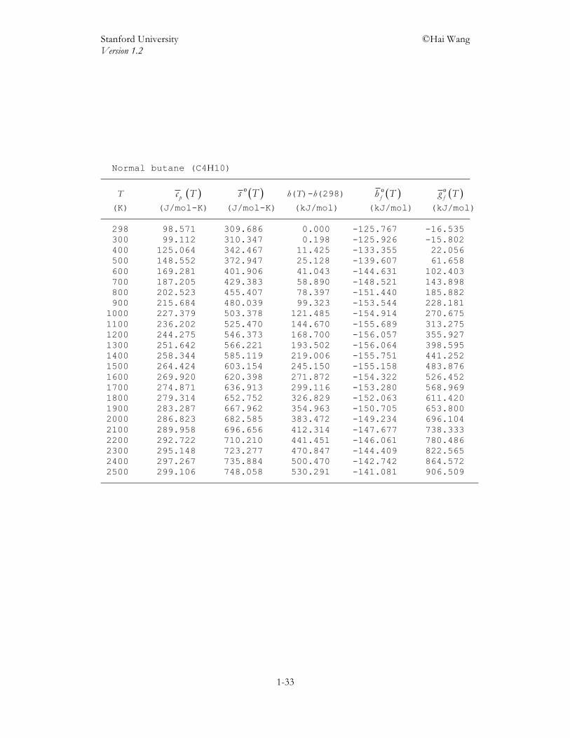
1-33

Normal butane (C4H10)


fg T

(K) (J/mol-K) (J/mol-K) (kJ/mol) (kJ/mol) (kJ/mol) 298 98.571 309.686 0.000 -125.767 -16.535 300 99.112 310.347 0.198 -125.926 -15.802 400 125.064 342.467 11.425 -133.355 22.056 500 148.552 372.947 25.128 -139.607 61.658 600 169.281 401.906 41.043 -144.631 102.403 700 187.205 429.383 58.890 -148.521 143.898 800 202.523 455.407 78.397 -151.440 185.882 900 215.684 480.039 99.323 -153.544 228.181 1000 227.379 503.378 121.485 -154.914 270.675 1100 236.202 525.470 144.670 -155.689 313.275 1200 244.275 546.373 168.700 -156.057 355.927 1300 251.642 566.221 193.502 -156.064 398.595 1400 258.344 585.119 219.006 -155.751 441.252 1500 264.424 603.154 245.150 -155.158 483.876 1600 269.920 620.398 271.872 -154.322 526.452 1700 274.871 636.913 299.116 -153.280 568.969 1800 279.314 652.752 326.829 -152.063 611.420 1900 283.287 667.962 354.963 -150.705 653.800 2000 286.823 682.585 383.472 -149.234 696.104 2100 289.958 696.656 412.314 -147.677 738.333 2200 292.722 710.210 441.451 -146.061 780.486 2300 295.148 723.277 470.847 -144.409 822.565 2400 297.267 735.884 500.470 -142.742 864.572 2500 299.106 748.058 530.291 -141.081 906.509


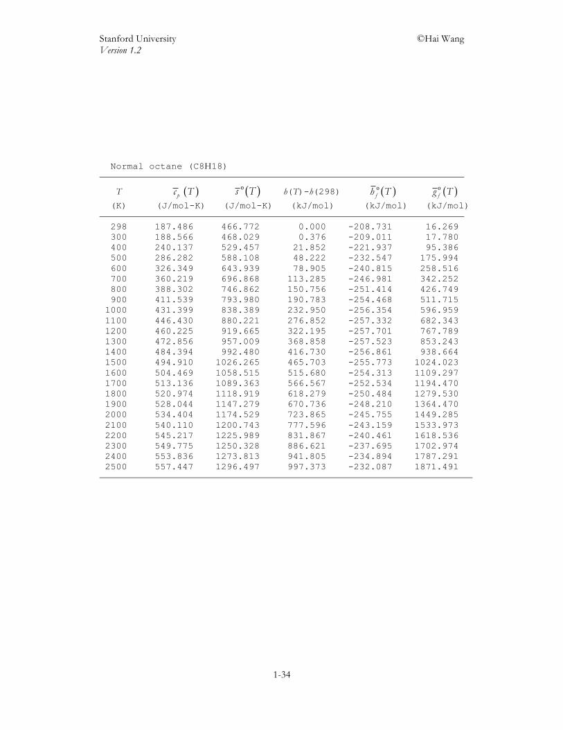
1-34

Normal octane (C8H18)


fg T

(K) (J/mol-K) (J/mol-K) (kJ/mol) (kJ/mol) (kJ/mol) 298 187.486 466.772 0.000 -208.731 16.269 300 188.566 468.029 0.376 -209.011 17.780 400 240.137 529.457 21.852 -221.937 95.386 500 286.282 588.108 48.222 -232.547 175.994 600 326.349 643.939 78.905 -240.815 258.516 700 360.219 696.868 113.285 -246.981 342.252 800 388.302 746.862 150.756 -251.414 426.749 900 411.539 793.980 190.783 -254.468 511.715 1000 431.399 838.389 232.950 -256.354 596.959 1100 446.430 880.221 276.852 -257.332 682.343 1200 460.225 919.665 322.195 -257.701 767.789 1300 472.856 957.009 368.858 -257.523 853.243 1400 484.394 992.480 416.730 -256.861 938.664 1500 494.910 1026.265 465.703 -255.773 1024.023 1600 504.469 1058.515 515.680 -254.313 1109.297 1700 513.136 1089.363 566.567 -252.534 1194.470 1800 520.974 1118.919 618.279 -250.484 1279.530 1900 528.044 1147.279 670.736 -248.210 1364.470 2000 534.404 1174.529 723.865 -245.755 1449.285 2100 540.110 1200.743 777.596 -243.159 1533.973 2200 545.217 1225.989 831.867 -240.461 1618.536 2300 549.775 1250.328 886.621 -237.695 1702.974 2400 553.836 1273.813 941.805 -234.894 1787.291 2500 557.447 1296.497 997.373 -232.087 1871.491


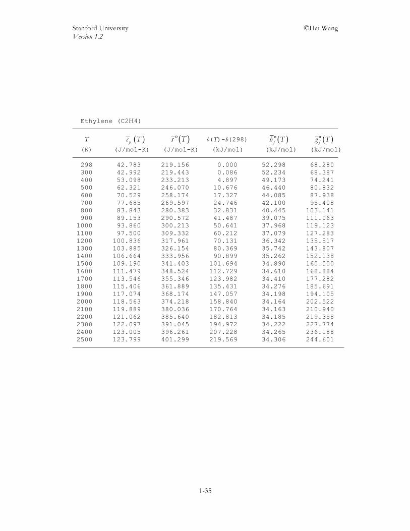
1-35

Ethylene (C2H4)


fg T



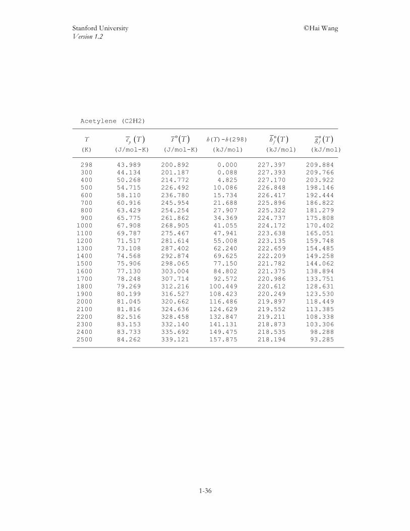
1-36

Acetylene (C2H2)


fg T



1-37

Methanol vapor (CH3OH(v))


fg T

(K) (J/mol-K) (J/mol-K) (kJ/mol) (kJ/mol) (kJ/mol) 298 44.030 239.785 0.000 -200.932 -162.241 300 44.155 240.080 0.088 -201.005 -161.981 400 51.400 253.735 4.852 -204.576 -148.427 500 59.526 266.074 10.397 -207.747 -134.013 600 67.334 277.628 16.746 -210.407 -119.008 700 74.146 288.534 23.830 -212.581 -103.597 800 79.807 298.817 31.536 -214.360 -87.902 900 84.681 308.502 39.764 -215.827 -72.003 1000 89.656 317.675 48.475 -216.987 -55.958 1100 93.611 326.410 57.642 -217.843 -39.811 1200 97.125 334.709 67.183 -218.487 -23.597 1300 100.239 342.608 77.054 -218.953 -7.336 1400 102.994 350.140 87.219 -219.269 8.955 1500 105.425 357.330 97.642 -219.463 25.264 1600 107.570 364.204 108.294 -219.556 41.583 1700 109.459 370.783 119.148 -219.571 57.905 1800 111.124 377.088 130.178 -219.523 74.226 1900 112.593 383.136 141.366 -219.429 90.543 2000 113.891 388.945 152.691 -219.301 106.854 2100 115.042 394.530 164.139 -219.151 123.158 2200 116.067 399.906 175.696 -218.987 139.455 2300 116.984 405.086 187.349 -218.817 155.744 2400 117.810 410.083 199.089 -218.647 172.025 2500 118.560 414.908 210.908 -218.482 188.300


1-38

Benzene (C6H6)


fg T



1-39

Hydrogen Atom (H•)


fg T



1-40

Oxygen atom (O•)


fg T



1-41

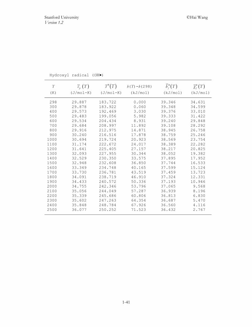
Hydroxyl radical (OH•)


fg T


Documents

Combustion Chemistry - Princeton University