Embed Size (px)
Citation preview

Copyright ©2016 by James F. Driscoll. This material is not to be sold, reproduced or distributed
without prior written permission of the owner, James F. Driscoll
Turbulent Combustion Experiments and Fundamental Models J. F. Driscoll, University of Michigan
Bell, Day, Driscoll
“corregated” premixed
R. Sankaran, E. Hawkes,
Jackie Chen T. Lu, C. K. Law
premixed
Wednesday: Non-premixed and Premixed Flames
1

Outline for the week
Mon: Physical concepts faster mixing, faster propagation, optimize liftoff, flame surface density, reaction rate, PDF Tues: Kilohertz PLIF, PIV measurements of flame structure - to assess models Wed: Non-Premixed and Premixed flames - measurements, models gas turbine example Thurs: Partially premixed flames - and some examples Fri: Future challenges: Combustion Instabilities (Growl) , Extinction
2

Assess JP-8 Chemistry ideas - of Hai Wang and others
3
“Lumped” Pyrolysis Model for JP-8
butane, ethylene butene, propene, etc.
Step #1: JP-8 breaks down into simpler fuels - but without any oxidation ( “lumped” = curve fit )
Step #2: the simpler fuels oxidize in ways that we understand
Detailed oxidation of each fuel
What are the limits to these approximations ?
Need turbulent flame experiments to give us the temperature time-history = realistic residence time in turbulent flames that represent real engines
Shock tube studies give the Arrhenius constants for these many reactions

Michigan Hi-Pilot Burner - now operated on methane and JP-8
4
21.6 mm 5 inch
co-flow
of OH
76 m/s vaporized JP-8
heating tape
fine spray
Delevan atomizer
liquid JP-8 from
Tim Edwards
Vaporized JP-8 at
ReT up to 99,000

pyrolysis zone
imaged with Jet-A PLIF
preheat region imaged with
formaldehyde PLIF
high T reaction zone
imaged with OH PLIF
CARS line imaging
of temperature, species
methane H2 Xi OH
Jet-A formaldehyde
toluene Xi OH
x x
CO
acetylene
CO2
ethylene
Fluorescence: 5 species (Michigan) CARS: 9 species (Gord, Meyer)
Imaging of pyrolysis layer - using vaporized JP-8 fuel
5

Pyrolysis images – how to assess chemistry model ?
Each laser shot (at 10 Hz) Simultaneously measure the profile of one species and temperature (CARS or LIF line imaging)
Jet-A Xi
x, mm
T
b) Convert x axis to temperature axis and plot data from different runs
c) Simultaneous 2-D PLIF images of pyrolysis layer, preheat, reaction layer to measure residence time = thickness / normal velocity
For residence time = 0.1 ms
Jet-A
6
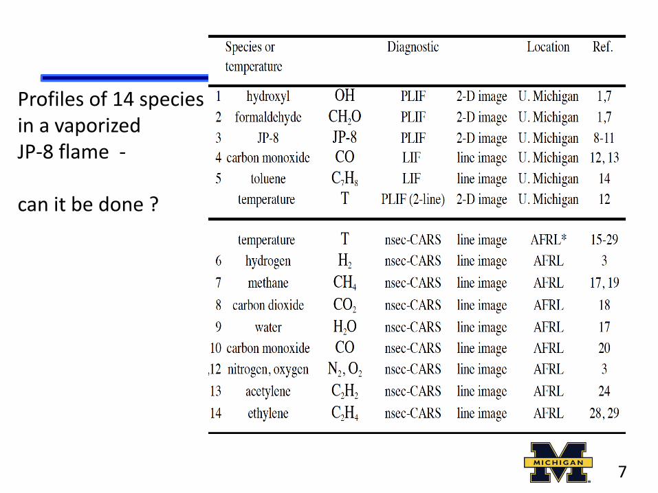
Profiles of 14 species in a vaporized JP-8 flame - can it be done ?
7
8
8. LIF of kerosene: Linne, M. et al., Optical Diagnostics AIAA J. 45, 11, 2007.
9. Fluorescence spectroscopy of kerosene: Grisch, F., Applied Phys. B 116, 729, 2014.
10. PLIF of Jet-A: Hochgreb, S. et al., J. Prop. Power 29,4, 961, 2013.
12. CO LIF: Barlow, R., Proc Comb Inst 32, 945, 2009
13. Temperature [CARS] and CO in Flames: Dreizler, A, Flow Turb Comb 90, 723, 2013.
14. LIF imaging of temperature [two line toluene] Sick, V et al, Proc Comb Inst 34, 3653
15. Gord, et al. 1-D thermometry in flames using CARS line imaging, Opt Let 36, 21
17. Gord, et al. [Review of CH4, H2, O2, N2 CARS] in PECS Vol. 36, p. 280
18. Gord, et al., CARS Temperature and CO2 Concentration, AIAA J. 41, 4, 679, 2003.
19. Meyer, T. et al [CH4, H2], Optics Lett 39, 23, 6608, 2014.
24. Gord, J. Detection of acetylene by CARS, Appl. Phys 87, 731, 2007.
“Evidence” that it can be done

9
Line CARS = coherent anti-Stokes Raman scattering - of Gord, AFRL
preheat
pyrolysis
primary reactions
laser “pump”
sheet
laser “probe”
sheet
CARS output light sheet to a camera 2 mm line
where species mass fractions are measured

Preheat temperatures (3) 300K, 500 K, 700 K (JP-8 cracks at 811 K) Pressures (3): 1 atm. (years 1 and 2), 10 atm. (in year 3) Reynolds number 80,000 for the highest case, is 16 times that of any previous burner
10
Results: line CARS at AFRL - Jim Gord

11
Future challenges - for Kilohertz laser diagnostics, LES and DNS
Highly unsteady combustion physics combustion instability (“growl”) structure of turbulent flames how to apply Law’s theory of flame stretch to highly turbulent flames ? Extinction, acceleration ? does Landau instability dominate turbulent wrinkling ? base of lifted jet flame – explain liftoff, blowout Use kilohertz wisely, use LES wisely - look at the dynamics, don’t just generate data !
Add heavy hydrocarbon chemistry to turbulent flame studies DNS: Blanquart (Cal Tech), Poludnenko (NRL), Bell (LBL), Jackie Chen (Sandia) Experiments: Ju (Princeton), Egolfopolous (USC) Your airplane flight here was not powered by methane - but by Jet-A !
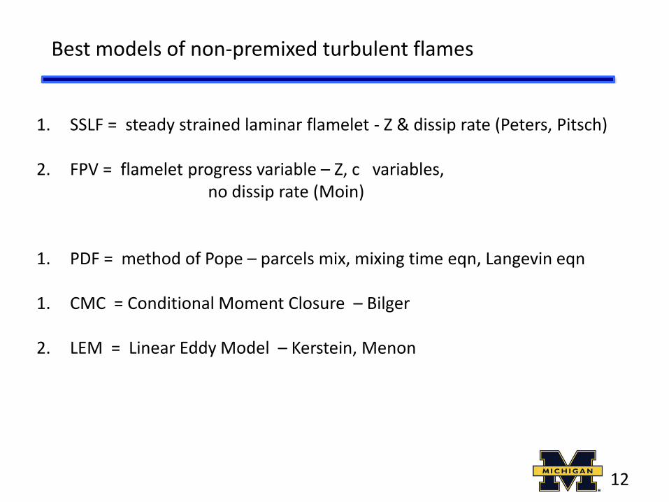
Best models of non-premixed turbulent flames
1. SSLF = steady strained laminar flamelet - Z & dissip rate (Peters, Pitsch)
2. FPV = flamelet progress variable – Z, c variables, no dissip rate (Moin)
1. PDF = method of Pope – parcels mix, mixing time eqn, Langevin eqn 1. CMC = Conditional Moment Closure – Bilger
2. LEM = Linear Eddy Model – Kerstein, Menon
12
13
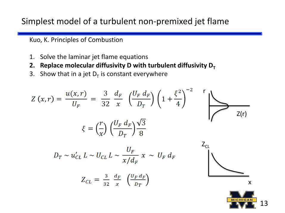
Simplest model of a turbulent non-premixed jet flame
Kuo, K. Principles of Combustion 1. Solve the laminar jet flame equations 2. Replace molecular diffusivity D with turbulent diffusivity DT
3. Show that in a jet DT is constant everywhere
ZCL
x
Z(r)
r

14
Mean radial velocity (v) - in simple jet model
v = mean radial velocity
radially inward radially outward
r
Flame location Set Z = Zst = 0.55 Plot eqn on previous slide
Flame length = flame location at r = 0, Lf = dF [constant/Zst]

Next level of modeling non-premixed turbulent Jet Flame – Unstrained flamelets Lockwood and Naguib, Comb. Flame 24, 109
8 unknowns, 8 equations
X - momentum
f - eqn
k equation
15
he defines mixture fraction as f ; it is the same as Z

epsilon equation g – equation Turbulent viscosity Lockwood assumes unstrained Laminar flamelets
16
17
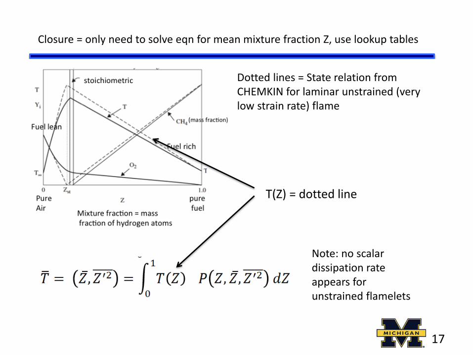
Dotted lines = State relation from CHEMKIN for laminar unstrained (very low strain rate) flame
Note: no scalar dissipation rate appears for unstrained flamelets
T(Z) = dotted line
Closure = only need to solve eqn for mean mixture fraction Z, use lookup tables
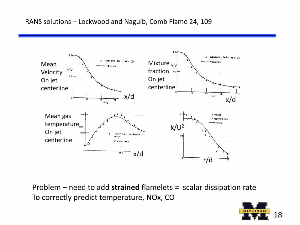
RANS solutions – Lockwood and Naguib, Comb Flame 24, 109
Mean Velocity On jet centerline
x/d
Mixture fraction On jet centerline
x/d
k/U2
r/d
Mean gas temperature On jet centerline
x/d
Problem – need to add strained flamelets = scalar dissipation rate To correctly predict temperature, NOx, CO
18

Non-premixed flames - add strained flamelets - Peters
Flamelet lookup tables – solve strained counterflow flame
Scalar Dissipation rate
Solid lines = state relations = CHEMKIN solutions to the strained flamelet equations with complex chemistry Two variables are mixture fraction and scalar dissipation rate
19

Counter flow non-premixed flame (Peters)
Assume: Laminar flow, fast chemistry For simplicity, assume constant density Velocity not disturbed by heat release All species diffuse at same diffusivity D Lewis number = 1, D = constant Scalars only vary in the y (vertical) direction So: u = e x ; v = -e y
Fuel
Air
20

Solution to this equation is:
y
Z(y)
For low strain rate e
Flame is at Z = Zs = 0.06
y
Z(y)
For high strain rate e
Larger gradient
Flame is at Z =Zs = 0.06
Scalar dissipation rate:
y
c (y)
at Flame
c = cs
cs = constant . e
21
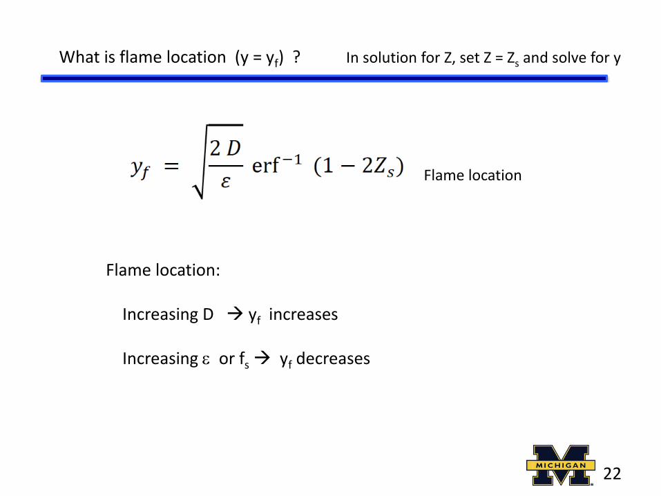
What is flame location (y = yf) ? In solution for Z, set Z = Zs and solve for y
Flame location: Increasing D yf increases Increasing e or fs yf decreases
Flame location
22

Strength of a strained non-premixed counterflow flame
Strength of a non-premixed flame = mass flux of fuel at flame boundary = JF = mass of fuel consumed /sec per unit flame area
Use our state relation that says that YF is proportional to Z on the fuel side of flame Take the derivative of the erf function formula for Z(y) Plug in our formula for y = yf at the flame front to get:
Stronger flame if strain rate e is made larger and e is Proportional to cst
23
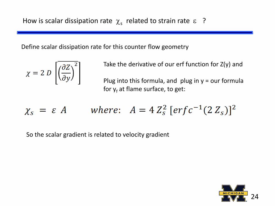
Define scalar dissipation rate for this counter flow geometry
How is scalar dissipation rate cs related to strain rate e ?
Take the derivative of our erf function for Z(y) and Plug into this formula, and plug in y = our formula for yf at flame surface, to get:
So the scalar gradient is related to velocity gradient
24

What is the thickness (df) of a strained non-premixed flame ?
Define the thickness of a non-premixed flame to be:
Take the derivative of our erf function for Z(y) and plug in our formula for yf to get:
Flame gets thinner as you apply more strain
Example: if D = 1.0 cm2/s = gas diffusivity near flame
if dissipation rate cs = 100 s-1
Then flame thickness: df = 1.4 mm
y
Z(y)
df
25

Steady non-premixed strained flamelet equation:
Solution yields state relations for all mass fractions, temperature, density as functions of Mixture fraction and Scalar dissipation rate
Now plug state relations into this to get mean values of temperature, density, mass fractions
instantaneous T, Yi are related to mixture fraction and dissipation rate in a turbulent flame in the same way they are related in a laminar counterflow flame with full chemistry
Flamelet assumption - of Peters adds strain to allow deviations from
equilibrium chemistry
26

State relations - for a strained non-premixed counter flow laminar flamelet
temperature
Mixture fraction Z
Dissipation rate cs = 25 s-1 50 s-1 100 s-1
YCO
Mixture fraction Z
Dissipation rate cs = 25 s-1 50 s-1 100 s-1
Generate plots above using CHEMKIN counter flow non-premixed flame solver Larger velocity gradient (strain rate) = larger scalar gradient (scalar dissipation rate) Larger dissipation rate lowers the peak temperature, alters the mass fractions of the species reduces the chemical reaction rate until extinction occurs improves prediction of CO, temperature, etc.
27

SSLF = Steady strained laminar flamelet LES model of Sandia Flame D by Janicka
Investigation of length scales, scalar dissipation, and flame orientation in a piloted diffusion flame by LES, A. Kempf J. Janicka PROCI 30 557
LES of Sandia flame D
Mixture fraction (Z) conservation eqn State relations from solutions to steady counter flow flamlet eqn Mean mix fraction in subgrid = prop. to resolved scale gradients of Z Variance of subgrid dissip. rate = prop. to resolved scale gradients Assume a Beta function for P(Z), log-normal for P(c). Mean quantities from:
state relation PDF
28

29
Janicka closure - for strained laminar flamelets
PDF of mixture fraction = Beta function, has mean and variance at each point PDF of scalar dissipation rate = log normal shape, has mean and variance At each (x,y,z) location we must compute the mean and variance of Z and c
Mean mixture fraction - from Z conservation equation Variance of mixture fraction - from “g” equation for scalar fluctuations Mean scalar dissipation rate – assumed to be proportional to epsilon (dissipation rate of turbulent kinetic energy), multiplied by the variance of mixture fraction sx is a constant, k and e come from the k and e equations, Variance of dissipation rate - assumed to be zero in FLUENT, others use an assumed algebraic equation
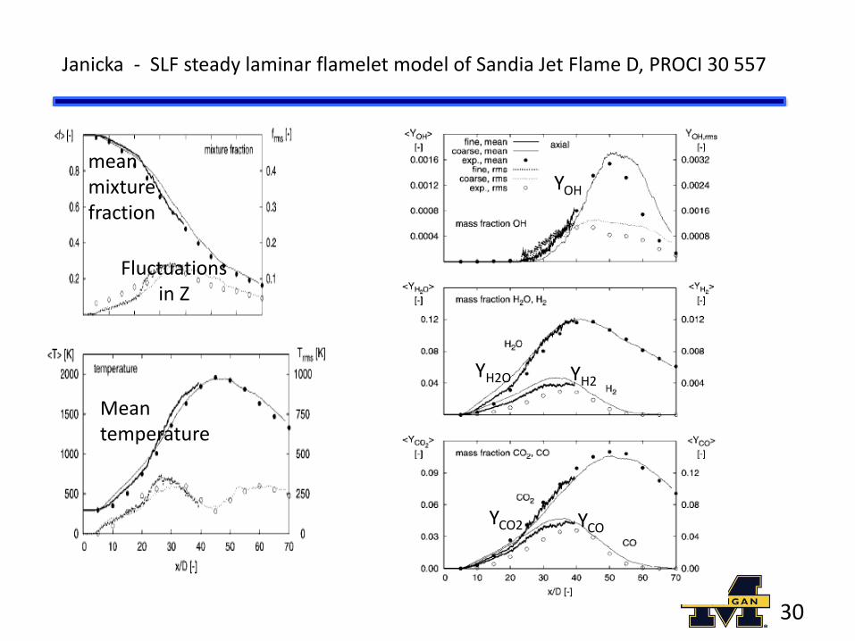
Janicka - SLF steady laminar flamelet model of Sandia Jet Flame D, PROCI 30 557
mean mixture fraction
Fluctuations in Z
Mean temperature
YOH
YH2O YH2
YCO2 YCO
30

Janicka SLF LES, continued
PDF of scalar dissipation rate Computed = bars Measured = dots
Conclude: the steady laminar flamelet LES adequately simulates the non-premixed combustion in Sandia jet flame D except for H2 and CO on the fuel rich side – it is a little off
31

Flamelet progress variable (FPV-LES) model - compared to Barlow’s
measurements in a non-premixed jet flame
C. Hasse, “LES flamelet-progress variable modeling and measurements of a turbulent partially-premixed dimethyl ether jet flame” Comb Flame 162, 3016
Progress variable: Yc = YH2 + YH2O + YCO + YCO2
Experiment Sandia flame D
LES of Hasse
OH
Formal dehyde
Replace scalar dissipation rate with a new progress variable Yc
32
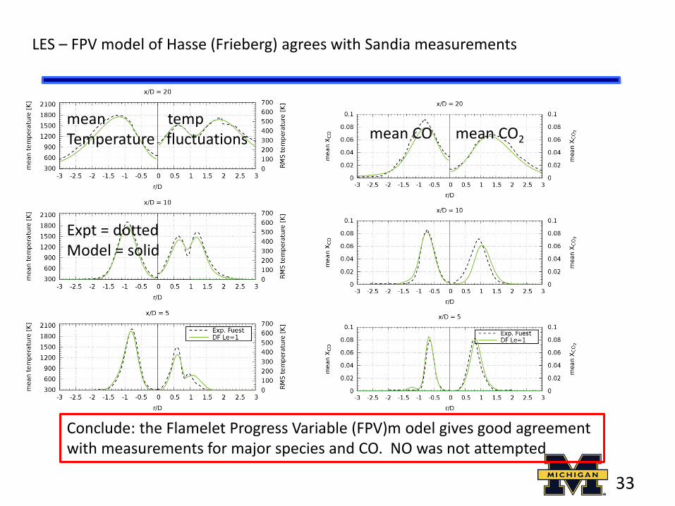
LES – FPV model of Hasse (Frieberg) agrees with Sandia measurements
mean temp Temperature fluctuations mean CO mean CO2
Expt = dotted Model = solid
Conclude: the Flamelet Progress Variable (FPV)m odel gives good agreement with measurements for major species and CO. NO was not attempted
33

Good Measurements – of non-premixed turbulent combustion
See TNF website http://www.sandia.gov/TNF/ Single point Raman/Rayleigh/LIF data for f, T, N2, O2, CH4, CO2, H2O, H2, CO, OH, NO and velocity
Barlow, R. S., Frank, J. H., A. N. Karpetis, and Chen, J.-Y., "Piloted Methane/Air Jet Flames: Scalar Structure and Transport Effects," Combust. Flame 143:433-449 (2005). Masri, A., Dibble, R.,Barlow, R., Structure of Turbulent Nonpremixed Flames Revealed by Raman-Rayleigh-LIF Measurements', Prog. Energy Combust. Sci., 22:307-362 (1997).
34

Barlow: Non-premixed piloted jet flame in Comb Flame 143, 433 and TNF website http://www.sandia.gov/TNF/ “Piloted methane/air jet flames: Transport effects and aspects of scalar structure”
Sandia flame D Jet diam. = 7.2 mm Pilot dia = 18.2 mm
Jet U = 50 m/s Coflow U = 0.9 m/s
Single point Raman/Rayleigh/LIF measurements of f, T, N2, O2, CH4, CO2, H2O, H2, CO, OH, NO, velocity, line Raman for scalar dissipation rate: Lasers for Raman, Rayleigh: Nd:YAG at 532 nm Lasers for LIF = Nd:YAG + dye: 282 nm for OH, 226 nm For NO, 230 nm for CO (two photon) Spatial resolution = 0.75 mm Fluorescence signals were corrected for Boltzmann fraction and collisional quenching rate
35

Barlow: Non-premixed jet flame in Comb Flame 143, 433
Data points = turbulent jet flame, Agree w steady laminar counterflow CHEMKIN = state relations computed for strain parameter 2 Uoo/R = 50 s-1
Conclude: steady flamelet state relations - Adequate for CO & major species - Not adequate for H2 or NO - Differential diffusion is negligible
36

PDF of mixture fraction is a Beta function
Max NO is near
stochiometric
Mixture Fraction
Scalar Diss rate
Barlow concludes: all important single point properties were measured in 5 piloted jet non-premixed flames, to be used to assess models
More Barlow measurements in turbulent non-premixed jet flames
37
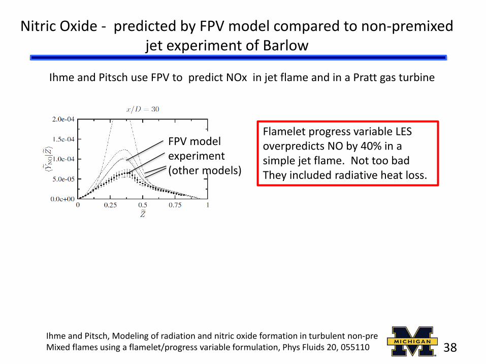
Nitric Oxide - predicted by FPV model compared to non-premixed jet experiment of Barlow
Ihme and Pitsch, Modeling of radiation and nitric oxide formation in turbulent non-pre Mixed flames using a flamelet/progress variable formulation, Phys Fluids 20, 055110
FPV model experiment (other models)
Flamelet progress variable LES overpredicts NO by 40% in a simple jet flame. Not too bad They included radiative heat loss.
Ihme and Pitsch use FPV to predict NOx in jet flame and in a Pratt gas turbine
38

NO can be predicted with post-processing (easy)
Ihme and Pitsch, Modeling of radiation and nitric oxide formation in turbulent non-pre Mixed flames using a flamelet/progress variable formulation, Phys Fluids 20, 055110
LES to compute temperature, YN2 and YO2 fields (means and variances)
NO is formed on long time scale so
We already know T, YO, YN2 from resolved scale LES
O + N2 NO + N etc.
State relation for wNO obtained from laminar flamelet eqn
39

Steinberg, A, , Meier, W. et al., Effects of Flow Structure Dynamics on Thermoacoustic Instabilities in Swirl-Stabilized Combustion, AIAA J. 50, p. 952.
5 kHz PLIF/PIV system
A more complex problem: gas turbine-like swirl flame undergoing
unsteady oscillations
40

41

What is the goal of comparing model results to experiments ?
Many models with very different assumptions all “agree” with measurements Is there any point in comparing output of models without assessing the basic assumptions in the model; i.e., do thin strained flamelets occur in the expt ? If models agree to within 5%, is there any point to work for better agreement ? Do we need to include heat losses, complex chemistry, acoustics, pressure ? Are computations really independent of b.c.s, initial condition, grid size ? Is the goal to identify the “best” model, or can we live with 20 models ? How useful are models that do not solve the Navier Stokes eqns ? Some replace NS with Langevin eqn, ad-hoc mixing models, etc. ?
42

Barlow, R. S., Frank, J. H., A. N. Karpetis, and Chen, J.-Y., "Piloted Methane/Air Jet Flames: Scalar Structure and Transport Effects," Combust. Flame 143:433-449 (2005) C. Hasse, “LES flamelet-progress variable modeling and measurements of a turbulent partially-premixed dimethyl ether jet flame” Comb Flame 162, 3016 Steinberg, A, , Meier, W. et al., Effects of Flow Structure Dynamics on Thermoacoustic Instabilities in Swirl-Stabilized Combustion, AIAA J. 50, p. 952.
Review of some good papers - in turbulent combustion
How are we doing ? How well are we making measurements and how well do models compare ?
43

How well can we model premixed turbulent flames ?
Assume thin or thickened wrinkled flamelets fully premixed or stratified premixed, FSD model is being modified to handle partially-premixed considers corregated (pockets) flamelet merging stretch rate increases area
Bray / FSD model
S = FSD
x
Masuya, Bray, Comb Sci Tech 25, 127
Gas temperature
Mean temperature
44
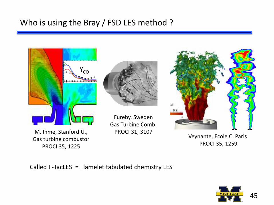
Who is using the Bray / FSD LES method ?
YCO
M. Ihme, Stanford U., Gas turbine combustor
PROCI 35, 1225
Veynante, Ecole C. Paris PROCI 35, 1259
Fureby. Sweden Gas Turbine Comb.
PROCI 31, 3107
Called F-TacLES = Flamelet tabulated chemistry LES
45

Reactedness = c is the fundamental parameter in premixed turbulent flames
Since r = p/RT, it follows that inserting the above in for T yields: r (c)= rR (c t +1)-1 where t = (TP/TR -1) = approx. 6 for typical flame
This is called a state relation for gas density as a function of c: r (c)
46

Probability density function - used to define a mean value
P(c) dc = probability that c lies in the range between c – dc/2 and c + dc/2
P
c
At each point in the flame, we solve conservation equations to get the mean and variance and plug into above eqn to get mean density
State relation: r (c)= rR (c t +1)-1
Idea: you only have to solve conservation equations for and and use above integral to get other mean values; you avoid solving more conservation equations for each variable
47
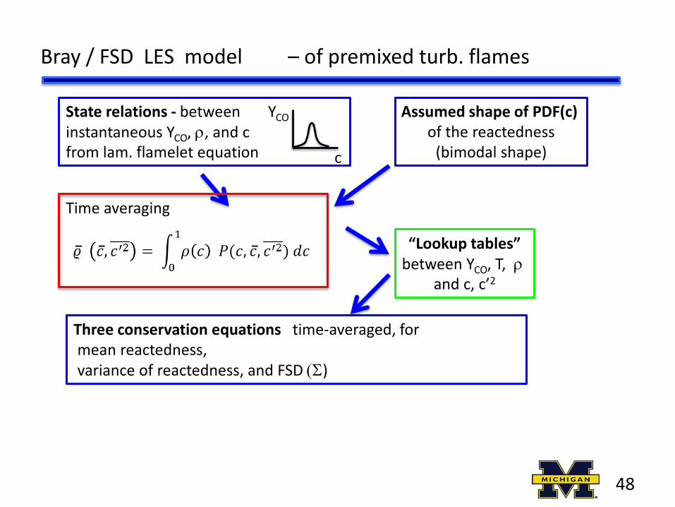
Bray / FSD LES model – of premixed turb. flames
Three conservation equations time-averaged, for mean reactedness, variance of reactedness, and FSD (S)
Assumed shape of PDF(c) of the reactedness
(bimodal shape)
“Lookup tables” between YCO, T, r
and c, c’2
State relations - between instantaneous YCO, r, and c from lam. flamelet equation
YCO
c
Time averaging
48

State relations - between instantaneous YCO, r, etc. and c from lam. flamelet equation
YCO
c
and YR = 1 – YP = 1 – c
Consider a 1-D, unstretched laminar premixed flame (see text by Law or Kuo, or solve using CHEMKIN)
c = reactedness YP = mass fraction products
We only have to solve ONE equation (the top one) for c(x) after we represent reaction rate of products in terms of c and YR
From c(x) we get T(x), r(x), YR(x), YP(x), YCH4(x), YH2O(x), etc.
for CH4 + 2 O2 + 2(79)/21 N2 2 H2O + CO2 + 2(79/21)N2
show that YCH4 = 0.062 YR = 0.062 (1-c) and YH2O = 0.12 YP = 0.12 c
49

State relations: between Yi , r, T and reactedness c
reactedness = c
1.0 0.0
YOH
formaldehyde
CHEMKIN PREMIXED LAMINAR
x (mm)
50
PREMIXED state relation from CHEMKIN premixed unstrained flamelet

Masuya, Bray, Comb Sci Tech 25, 127, 1981
x
= rR (1-c) SL S
rate of temperature rise in x direction
turbulent flux of temperature fluctuations
volumetric reaction rate kg/s of products /m3
(kg/m3) (m/s) (1/m) = (kg/m2/s) (area/vol)
reaction rate/area
Conservation of mean reactedness
Conservation of scalar flux
Goal: Two ODEs for the unknowns and
51

Bi - Modal PDF for a premixed flame (Bray)
P(u,c) = A(u) d(c) + B(u) d(1-c)
d(c) is delta fcn centered at c = 0 d(1-c) is delta fcn centered at c = 1 A(u) and B(u) are Gaussian dist. of velocity Areas under Gaussians A + B = 1 Mean of A(u) is mean velocity of reactants Variance of A(u) is variance of reactants Mean of B(u) is mean velocity of products Variance of B(u) is variance of products
52

Mean CO2 mass fraction depends only on two quantities that are computed at each (x,y,z) location using conservation equations for these two quantities
State relation YCO2 is a known fraction of YP which equals c
“Lookup tables” between YH2O, T, r
and
53

Relate all quantities in the two conservation equations to the two unknowns
and
There are no fluctuations in reactedness or temperature in the pure reactants or in the pure products
example
Bimodal PDF: P(c) = A d(c-0) + B d(c-1)
54

Bray model closure – still have flame surface density S (x) in conservation eqn
x
S ?
Third conservation equation must be solved for FSD = S
S is proportional to turbulent reaction rate
Final step: specify correct boundary conditions and solve for = ST
= turbulent burning velocity
Flame Surface Density Conservation Equation
55

Bray / FSD LES model – of premixed turb. flames
Conservation equations time-averaged, for mean reactedness turbulent flux of reactedness flame surface density (S), is prop. to mean reaction rate
Assumed shape of PDF(c) of the reactedness
(bimodal shape)
“Lookup tables” between YCO, T, r
and c, c’2
Time averaging
State relations - between instantaneous YCO, r, and c from lam. flamelet equation
YCO
c
56

Bray / FSD model applied to premixed jet flame Prasad and Gore Comb Flame 116,1
Flame Surface Density for S
TKE for k, e
Conclude: model predicts correct flame height and turbulent burning velocity (if appropriate constants are selected !)
Mean Temp.
(K)
2000 1000 300
r (mm)
Axial mom. For
Continuity For
Mean Reactedness
57

F-TacLES is Multi-variable approach - for stratified premixed
Consider a “stratified” premixed flame - equivalence ratio varies in the reactants Define Z = mixture fraction = mass fraction of H atoms at a point Ex. If mixture is CH4 + ½ H2O then Z = 5 / (16 +9) = 0.2
Filtered TAbulated Chemistry for LES (F-TACLES)
58

Premixed F-TACLES LES model
“The influence of combustion SGS submodels on the resolved flame propagation. application to the LES of the Cambridge stratified flames” R. Mercier , T. Schmitt, D. Veynante, B. Fiorina, PROCI 35, 1259 Filtered TAbulated Chemistry for LES (F-TACLES) model propagates resolved flame at the subgrid scale turbulent flame speed ST,D
Solves for mean progress variable
= new flame surface density parameter
59
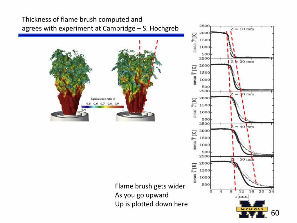
Flame brush gets wider As you go upward Up is plotted down here
Thickness of flame brush computed and agrees with experiment at Cambridge – S. Hochgreb
60