Colorado School of Mines CHEN403 Laplace …inside.mines.edu/~jjechura/ProcessDynamics/05_LaplaceTransforms.pdfColorado School of Mines CHEN403 Laplace Transforms . = = = . ¦ ¦ ¦

Colorado School of Mines CHEN403 Laplace Transforms

John Jechura ([email protected]) - 1 - © Copyright 2017

April 23, 2017

Laplace Transforms

Laplace Transforms ................................................................................................................................................. 1

Definition of the Transform ................................................................................................................................. 2

Properties of Laplace Transform ....................................................................................................................... 2

Transforms of Simple Functions ........................................................................................................................ 3

Translation of Transforms ................................................................................................................................... 5

Transforms of Derivatives .................................................................................................................................... 6

Transforms of Integrals ......................................................................................................................................... 6

Final-Value & Initial-Value Theorems ............................................................................................................. 7

Inverse Laplace Transform — Conversion to Partial Fractions .......................................................... 8

Collection of Terms ............................................................................................................................................. 9

Specific Values of s .......................................................................................................................................... 11

Heaviside Expansion Method ...................................................................................................................... 12

More Complicated Partial Fractions – Repeated Roots ........................................................................ 13

Heaviside Expansion for Repeated Roots .............................................................................................. 14

Specific s Values for Repeated Roots ....................................................................................................... 14

More Complicated Partial Fractions – Quadratic & Higher Order Terms ..................................... 15

Repeated Roots .................................................................................................................................................. 15

Complex Conjugate Roots ............................................................................................................................. 16

Inverting Quadratic Term – Completing the Square .............................................................................. 19

Steps for Completing the Square ............................................................................................................... 19

Example #1 .......................................................................................................................................................... 20

Numerical Root Finding & Partial Fractions.............................................................................................. 21

All Real Roots ..................................................................................................................................................... 21

Complex Conjugate Roots ............................................................................................................................. 23

Solution of Initial Value ODEs .......................................................................................................................... 27

Solution of Systems of Initial Value ODEs ................................................................................................... 28

Translation of Transform ................................................................................................................................... 31

Further Examples — Finding Transform of Piece-Wise Driving Function .................................. 32

Further Examples — Inverse Transform With Time Delay ................................................................ 34

Further Examples — Arbitrary Driving Function in ODE .................................................................... 36

Use of Mathematical Software to Work with Laplace Transforms .................................................. 39

Mathematica ....................................................................................................................................................... 39

MATLAB ................................................................................................................................................................ 42

Microsoft Excel .................................................................................................................................................. 46

POLYMATH .......................................................................................................................................................... 50

Laplace transforms provide an efficient way to solve linear differential equations with constant coefficients. These are traditional method to solve process control problems. Use

algebra instead of calculus.



April 23, 2017

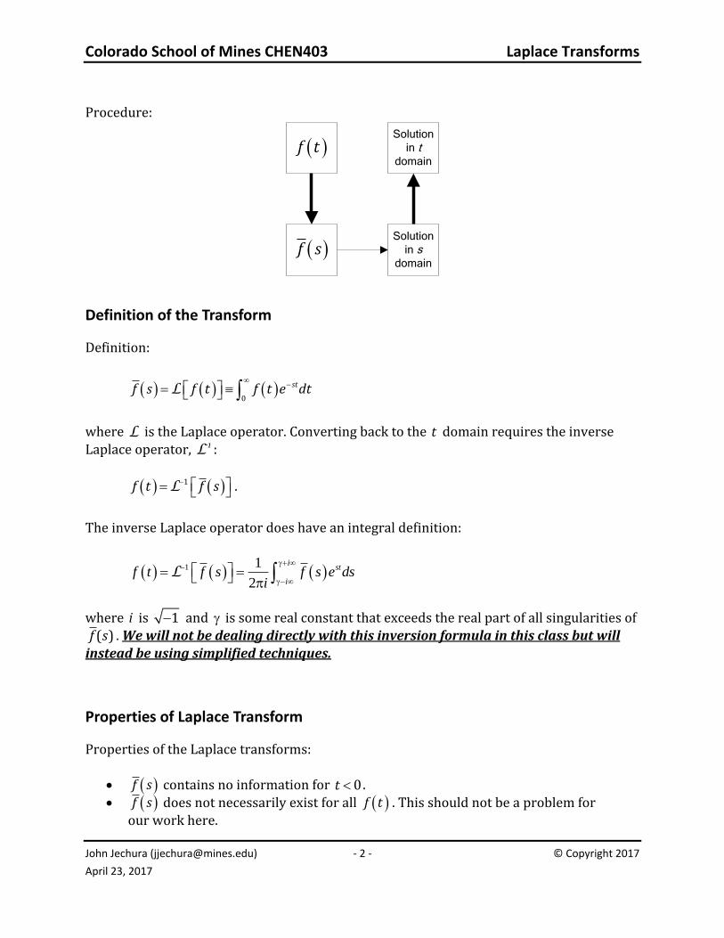
Procedure:

f tSolution

in t domain

f sSolution

in s

domain

Definition of the Transform

Definition:

0stf s f t f t e dtL

where L is the Laplace operator. Converting back to the t domain requires the inverse Laplace operator, -1L :

1f t f sL .

The inverse Laplace operator does have an integral definition:

1 1

2

ist

if t f s f s e ds

i

L

where i is 1 and is some real constant that exceeds the real part of all singularities of

( )f s . We will not be dealing directly with this inversion formula in this class but will instead be using simplified techniques.

Properties of Laplace Transform

Properties of the Laplace transforms:

• f s contains no information for 0t . • f s does not necessarily exist for all f t . This should not be a problem for

our work here.



April 23, 2017

• L is linear:

1 2 1 2af t bf t a f t b f tL L L

• L removes the t variable by integration but replaces it with s .

Proof of linearity:

1 2 1 20

1 20 0

1 2

st

st st

af t bf t af t bf t e dt

a f t e dt b f t e dt

a f t b f t

L

L L

Example of function with transform — let atf t e where 0a . f s only exists when

0a s , since:

0 0

a s tat at ste e e dt e dtL

Transforms of Simple Functions

Common transforms shown in the text book. There are 99 functions listed on pp. 296-299 of Handbook of Mathematical Formulas and Integrals. The most needed in this class are part of these notes. Let’s derive some of them. First, we need to remember how to integrate by parts. Since:

d uv udv vdu udv d uv vdu

then, the integration gives us:

udv d uv vdu udv uv vdu

and: b bb

aa audv uv vdu



April 23, 2017

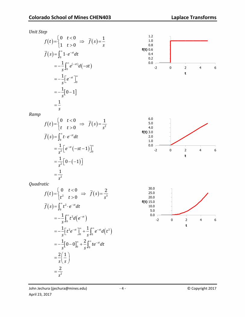
Unit Step

0 0 1

1 0

tf t f s

t s

0

0

0

1

1

1

10 1

1

st

st

st

f s e dt

e d sts

es

s

s

0.0

0.2

0.4

0.6

0.8

1.0

1.2

-2 0 2 4 6

t

f(t)

Ramp

2

0 0 1

0

tf t f s

t t s

0

2 0

2

2

11

10 1

1

st

st

f s t e dt

e sts

s

s

0.0

1.0

2.0

3.0

4.0

5.0

6.0

-2 0 2 4 6

t

f(t)

Quadratic

2 3

0 0 2

0

tf t f s

t t s

2

0

2

0

2 2

0 0

0 0

2

1

1 1

1 20 0

2 1

2

st

st

st st

st

f s t e dt

t d es

t e e d ts s

te dts s

s s

s

0.0

5.0

10.0

15.0

20.0

25.0

30.0

-2 0 2 4 6

t

f(t)



April 23, 2017

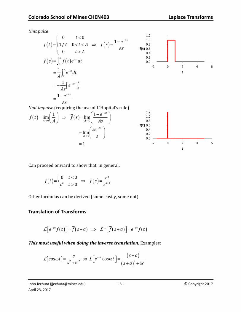
Unit pulse

0 01

1/ 0

0

Ast

ef t A t A f s

Ast A

0

0

0

1

1

1

st

Ast

Ast

As

f s f t e dt

e dtA

eAs

e

As

0.0

0.2

0.4

0.6

0.8

1.0

1.2

-2 0 2 4 6

t

f(t)

Unit impulse (requiring the use of L’Hopital’s rule)

0 0

0

1 1lim lim

lim

1

As

A A

As

A

ef t f s

A As

se

s

0.0

0.2

0.4

0.6

0.8

1.0

1.2

-2 0 2 4 6

t

f(t)

Can proceed onward to show that, in general:

1

0 0 !

0n n

t nf t f s

t t s

Other formulas can be derived (some easily, some not).

Translation of Transforms

1at ate f t f s a f s a e f tL L

This most useful when doing the inverse translation. Examples:

2 2

coss

ts

L so

2 2

cosat s ae t

s aL



April 23, 2017

2

1f s

s a — since 2

1t

sL , then

1

2

1 attes a

L

Transforms of Derivatives

0df t

sf s fdt

L

2

2

20

0t

d f t dfs f s sf

dt dtL

3 23 2

3 20 0

0t t

d f t df d fs f s s f s

dt dt dtL

2 11 2

2 10 0 0

0n n n

n n n

n n nt t t

d f t df d f d fs f s s f s s

dtdt dt dtL

Note that we can change an n-th order ODE in t into an n-th order polynomial in s . This is why Laplace transforms have been used.

Also note that for an n-th order ODE in t we need n initial conditions: 0f , 0

/t

df dt , …,

1 1

0/

n n

td f dt .

Proof of transform of 1st derivative using integration by parts:

0

0

0 0

00 0

0

st

st

st st

st

df t df te dt

dt dt

e df t

e f t f t d e

f s f t e dt

f sf s

L

Transforms of Integrals

0

1t

f d f ss

L



April 23, 2017

Proof:

0 0 0

0 0

0 0 00

0

0 0 0

1

1 1

1 1

1 10 0

1

t tst

tst

t tst st

st

f d f d e dt

f d d es

e f d e d f ds s

e f d f d f t e dts s

f ss s

f ss

L

Final-Value & Initial-Value Theorems

0lim limt s

f t s f s for f s that exists over the entire range of 0 s .

0lim limt s

f t s f s

With these two theorems, we can determine the limiting values of a function only knowing the Laplace transform. Example #1:

6

1 2 3

sf s

s s s s

0

6 6lim lim 1

1 2 3 6t s

sf t

s s s

2

0

1 61

6lim lim lim 0

1 2 31 2 31 1 1

t s s

s s sf t

s s s

s s s

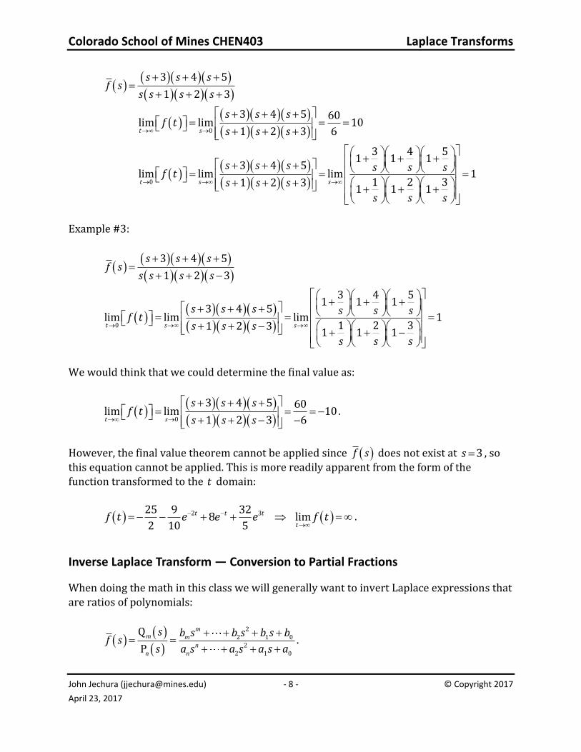
Example #2:



April 23, 2017

3 4 5

1 2 3

s s sf s

s s s s

0

3 4 5 60lim lim 10

1 2 3 6t s

s s sf t

s s s

0

3 4 51 1 1

3 4 5lim lim lim 1

1 2 31 2 31 1 1

t s s

s s s s s sf t

s s s

s s s

Example #3:

3 4 5

1 2 3

s s sf s

s s s s

0

3 4 51 1 1

3 4 5lim lim lim 1

1 2 31 2 31 1 1

t s s

s s s s s sf t

s s s

s s s

We would think that we could determine the final value as:

0

3 4 5 60lim lim 10

1 2 3 6t s

s s sf t

s s s.

However, the final value theorem cannot be applied since f s does not exist at 3s , so this equation cannot be applied. This is more readily apparent from the form of the function transformed to the t domain:

2 325 9 32

8 lim2 10 5

t t t

tf t e e e f t .

Inverse Laplace Transform — Conversion to Partial Fractions

When doing the math in this class we will generally want to invert Laplace expressions that are ratios of polynomials:

22 1 0

22 1 0

Q

P

mm m

nn n

s b s b s b s bf s

s a s a s a s a.



April 23, 2017

We will invert the Laplace transforms by matching forms in tables. The functions we want to invert are generally more complicated than those listed in the reference tables. We can do this by splitting up the Laplace function in terms of partial fractions, each of which can be matched up to the tables. There are three techniques to break the Laplace function apart

into partial fractions: 1. Collection of Terms 2. Specific Values of s . 3. Heaviside Expansion.

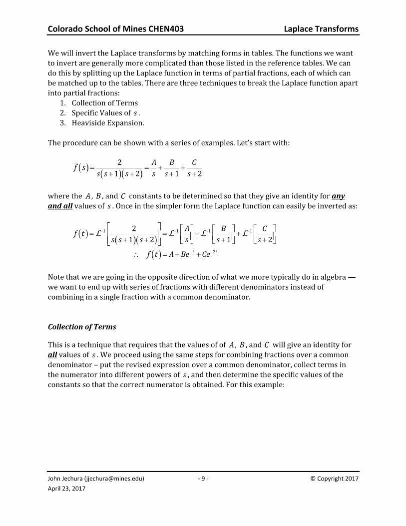
The procedure can be shown with a series of examples. Let’s start with:

2

1 2 1 2

A B Cf s

s s s s s s

where the A , B , and C constants to be determined so that they give an identity for any and all values of s . Once in the simpler form the Laplace function can easily be inverted as:

1 1 1 1

2

2

1 2 1 2

t t

A B Cf t

s s s s s s

f t A Be Ce

L L L L

Note that we are going in the opposite direction of what we more typically do in algebra — we want to end up with series of fractions with different denominators instead of combining in a single fraction with a common denominator. Collection of Terms

This is a technique that requires that the values of of A , B , and C will give an identity for all values of s . We proceed using the same steps for combining fractions over a common denominator – put the revised expression over a common denominator, collect terms in the numerator into different powers of s , and then determine the specific values of the constants so that the correct numerator is obtained. For this example:



April 23, 2017

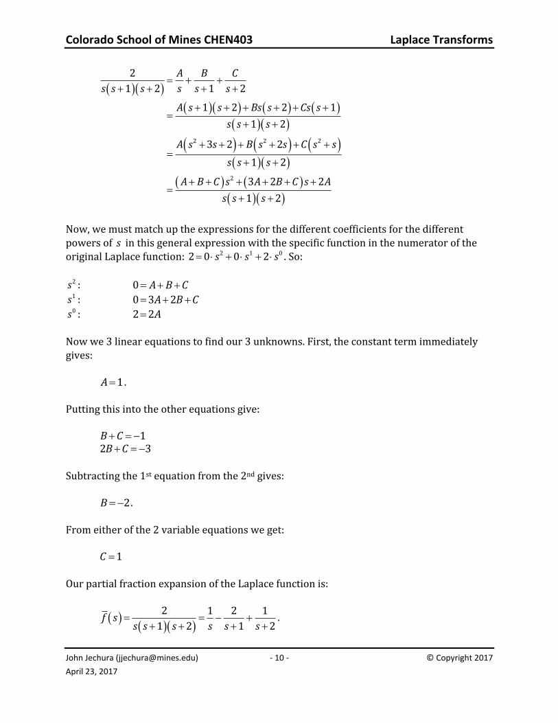
2 2 2

2

2

1 2 1 2

1 2 2 1

1 2

3 2 2

1 2

3 2 2

1 2

A B C

s s s s s s

A s s Bs s Cs s

s s s

A s s B s s C s s

s s s

A B C s A B C s A

s s s

Now, we must match up the expressions for the different coefficients for the different powers of s in this general expression with the specific function in the numerator of the original Laplace function: 2 1 02 0 0 2s s s . So:

2s : 0 A B C 1s : 0 3 2A B C 0s : 2 2A

Now we 3 linear equations to find our 3 unknowns. First, the constant term immediately gives: 1A . Putting this into the other equations give: 1B C 2 3B C Subtracting the 1st equation from the 2nd gives: 2B . From either of the 2 variable equations we get: 1C Our partial fraction expansion of the Laplace function is:

2 1 2 1

1 2 1 2f s

s s s s s s.



April 23, 2017

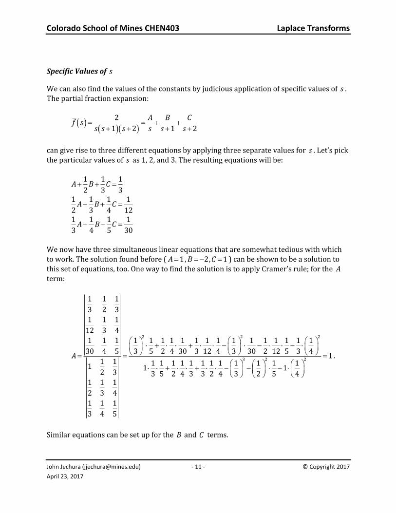
Specific Values of s

We can also find the values of the constants by judicious application of specific values of s . The partial fraction expansion:

2

1 2 1 2

A B Cf s

s s s s s s

can give rise to three different equations by applying three separate values for s . Let’s pick the particular values of s as 1, 2, and 3. The resulting equations will be:

1 1 1

2 3 3A B C

1 1 1 1

2 3 4 12A B C

1 1 1 1

3 4 5 30A B C

We now have three simultaneous linear equations that are somewhat tedious with which to work. The solution found before ( 1A , 2B , 1C ) can be shown to be a solution to

this set of equations, too. One way to find the solution is to apply Cramer’s rule; for the A term:

2 2 2

3 2 2

1 1 1

3 2 3

1 1 1

12 3 4

1 1 1 1 1 1 1 1 1 1 1 1 1 1 1 1 1 1

30 4 5 3 5 2 4 30 3 12 4 3 30 2 12 5 3 41

1 1 1 1 1 1 1 1 1 1 1 1 1 11 1 12 3 3 5 2 4 3 3 2 4 3 2 5 4

1 1 1

2 3 4

1 1 1

3 4 5

A .

Similar equations can be set up for the B and C terms.



April 23, 2017

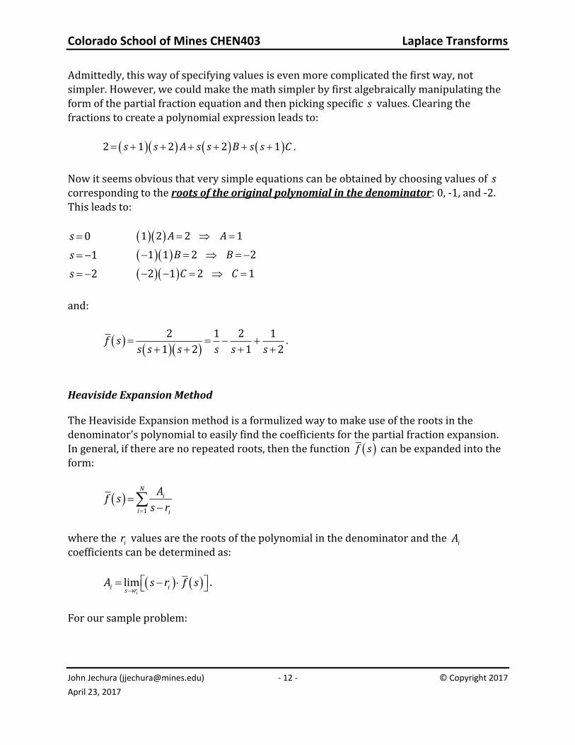
Admittedly, this way of specifying values is even more complicated the first way, not simpler. However, we could make the math simpler by first algebraically manipulating the form of the partial fraction equation and then picking specific s values. Clearing the fractions to create a polynomial expression leads to:

2 1 2 2 1s s A s s B s s C .

Now it seems obvious that very simple equations can be obtained by choosing values of s corresponding to the roots of the original polynomial in the denominator: 0, -1, and -2. This leads to:

0s 1 2 2 1A A

1s 1 1 2 2B B

2s 2 1 2 1C C

and:

2 1 2 1

1 2 1 2f s

s s s s s s.

Heaviside Expansion Method

The Heaviside Expansion method is a formulized way to make use of the roots in the denominator’s polynomial to easily find the coefficients for the partial fraction expansion. In general, if there are no repeated roots, then the function f s can be expanded into the form:

1

Ni

i i

Af s

s r

where the ir values are the roots of the polynomial in the denominator and the iA coefficients can be determined as:

limi

i is r

A s r f s .

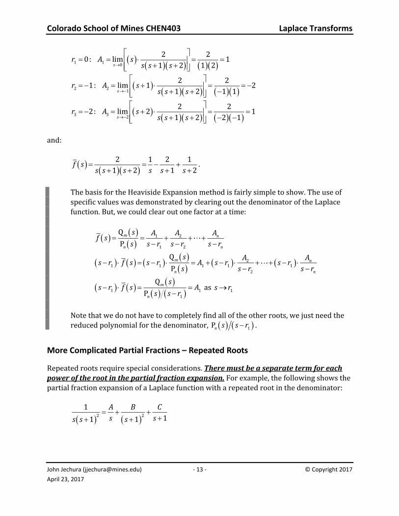
For our sample problem:



April 23, 2017

1 1

0

2 20: lim 1

1 2 1 2sr A s

s s s

2 2

1

2 21: lim 1 2

1 2 1 1sr A s

s s s

3 3

2

2 22: lim 2 1

1 2 2 1sr A s

s s s

and:

2 1 2 1

1 2 1 2f s

s s s s s s.

The basis for the Heaviside Expansion method is fairly simple to show. The use of specific values was demonstrated by clearing out the denominator of the Laplace function. But, we could clear out one factor at a time:

1 2

1 2

Q

Pm n

n n

s A A Af s

s s r s r s r

21 1 1 1 1

2

Q

Pm n

n n

s A As r f s s r A s r s r

s s r s r

1 1

1

Q

Pm

n

ss r f s A

s s r as 1s r

Note that we do not have to completely find all of the other roots, we just need the reduced polynomial for the denominator, 1Pn s s r .

More Complicated Partial Fractions – Repeated Roots

Repeated roots require special considerations. There must be a separate term for each power of the root in the partial fraction expansion. For example, the following shows the partial fraction expansion of a Laplace function with a repeated root in the denominator:

2 2

1

11 1

A B C

s ss s s



April 23, 2017

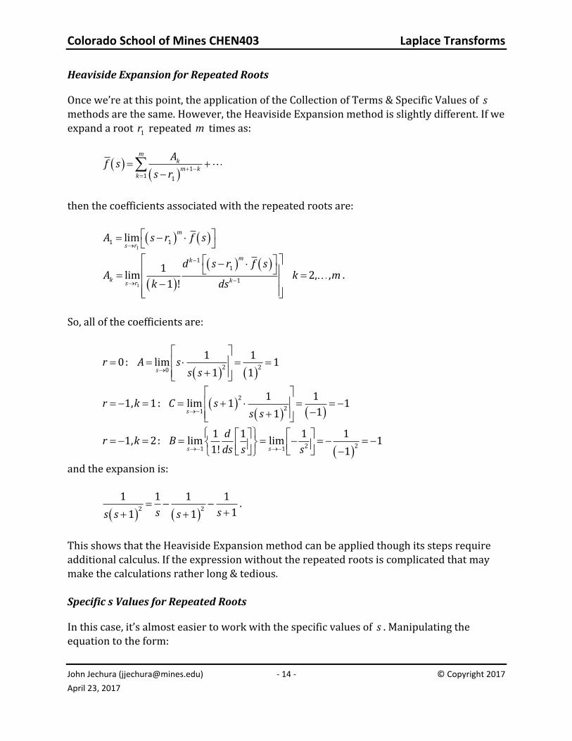
Heaviside Expansion for Repeated Roots

Once we’re at this point, the application of the Collection of Terms & Specific Values of s methods are the same. However, the Heaviside Expansion method is slightly different. If we

expand a root 1r repeated m times as:

11 1

mk

m kk

Af s

s r

then the coefficients associated with the repeated roots are:

1

1 1limm

s rA s r f s

1

11

1

1lim 2, ,

1 !

mk

k ks r

d s r f sA k m

k ds.

So, all of the coefficients are:

2 20

1 10: lim 1

1 1sr A s

s s

2

21

1 11, 1: lim 1 1

11sr k C s

s s

221 1

1 1 1 11, 2: lim lim 1

1! 1s s

dr k B

ds s s

and the expansion is:

2 2

1 1 1 1

11 1s ss s s.

This shows that the Heaviside Expansion method can be applied though its steps require additional calculus. If the expression without the repeated roots is complicated that may make the calculations rather long & tedious. Specific s Values for Repeated Roots

In this case, it’s almost easier to work with the specific values of s . Manipulating the equation to the form:



April 23, 2017

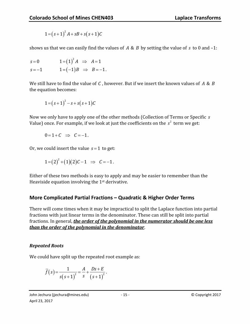
2

1 1 1s A sB s s C

shows us that we can easily find the values of A & B by setting the value of s to 0 and –1:

0s 2

1 1 1A A

1s 1 1 1B B .

We still have to find the value of C , however. But if we insert the known values of A & B the equation becomes:

2

1 1 1s s s s C

Now we only have to apply one of the other methods (Collection of Terms or Specific s Value) once. For example, if we look at just the coefficients on the 2s term we get: 0 1 1C C .

Or, we could insert the value 1s to get:

2

1 2 1 2 1 1C C .

Either of these two methods is easy to apply and may be easier to remember than the Heaviside equation involving the 1st derivative.

More Complicated Partial Fractions – Quadratic & Higher Order Terms

There will come times when it may be impractical to split the Laplace function into partial fractions with just linear terms in the denominator. These can still be split into partial fractions. In general, the order of the polynomial in the numerator should be one less than the order of the polynomial in the denominator. Repeated Roots

We could have split up the repeated root example as:

2 2

1

1 1

A Ds Ef s

ss s s.



April 23, 2017

The manipulated polynomial form for this is now:

2

1 1s A s Ds E .

We have a myriad of ways to determine the value of A . Setting s to the root value of 0 gives:

2

1 1 1A A .

Now however setting s to the other root value of -1 not give one of the other coefficients but rather a relationship:

1s : 1 1 1D E D E .

Setting s to one gives another relationship (remembering to include the A term):

1s : 2

1 2 1 1 1 3D E D E .

Adding the two relationships together gives: 2 2 1D D

and we can derive 2E from either relationship. Now the expansion is:

2 2

1 1 2

1 1

sf s

ss s s.

With a little more manipulation this can also be expressed as:

2 2 2 2 2

1 1 2 1 1 1 1 1 1

11 1 1 1 1

s sf s

s s s ss s s s s s

the same expression we found before. Complex Conjugate Roots

This technique is used most useful when there is a quadratic term with complex conjugate roots. For example, the quadratic term:



April 23, 2017

2

1

2 2f s

s s s

cannot be split into real factors (since it has complex conjugate roots). Using only real arithmetic it can be split as:

22

1

2 22 2

A Ds Ef s

s s ss s s.

We can still determine A using the Heaviside Method (or one of the other methods):

20

1 1 10: lim

1 2 22 2sr A s

s s s

leaving the equation:

22

1 1 1

2 2 22 2

Ds Ef s

s s ss s s.

We can manipulate the Laplace function to form the polynomial:

22 2 2 2s s s Ds E ;

we can determine D and E using the specific values of 1 and -1 for s :

2 2 3 1/2

2 2 1 1

D E D

D E E

giving:

22

1 1 1 1 2

2 2 2 22 2

sf s

s s ss s s.

If we’re willing to use complex arithmetic then we can work directly with the complex factors:



April 23, 2017

2

1

1 12 2

A B Cf s

s s i s is s s

where 1i . The Heaviside Method can be used to find the coefficients even for

complex roots:

1

11 : lim 1

1 1

1

1 1 1

1

1 2

1 2 2

2 2 2 2

2 2

4 4

1

4

s ir i B s i

s s i s i

i i i

i i

i

i i

i

i

1

11 : lim 1

1 1

1

1 1 1

1

1 2

1 2 2

2 2 2 2

2 2

4 4

1

4

s ir i C s i

s s i s i

i i i

i i

i

i i

i

i

So, the partial fraction form of this Laplace function is:

2

1 1 1 1 1 1 1

2 4 1 4 12 2

i if s

s s i s is s s.



April 23, 2017

Inverting Quadratic Term – Completing the Square

Will generally want to expand a quadratic (or higher polynomial) in the denominator as product of linear terms. However, we may instead want to “complete the square” and use

different translations of the transform function. A particularly simple example is:

2

1 1 1 1

8 7 7 1 6 1 6 7f s

s s s s s s

71 1

6 6t tf t e e .

We could also “complete the square” to get:

2 22 2 2 2

1 1 1 1 3

8 7 38 16 9 4 3 4 3f s

s s s s s s

41sinh 3

3tf t e t .

Note that these expressions are equivalent since sinh /2x xx e e , so:

3 3 74 41 1

sinh 33 3 2 6

t t t tt t e e e e

e t e

Completing the square is much more important when the quadratic cannot be factored into real roots (i.e., has complex conjugate roots). For the quadratic used in the previous example:

22 2

1 1

2 2 1 1f s

s s s

sintf t e t .

Steps for Completing the Square

The key step in completing the square is to determine half the value of the coefficient of the s term. We then want to split this value squared out of the constant term. Overall, we want to manipulate the quadratic into the following form:

• Identify half the value of the coefficient on the s term – express the quadratic as:



April 23, 2017

2 2s Bs C . • Separate out the square of half the value of the coefficient from the constant term:

2 2 22s Bs B C B .

• Express the quadratic term as a square:

2 2s B C B .

• Express the constant term as a square of its absolute value – be mindful that the sign

of the resulting term should match the sign of this difference:

2

2 2s B C B .

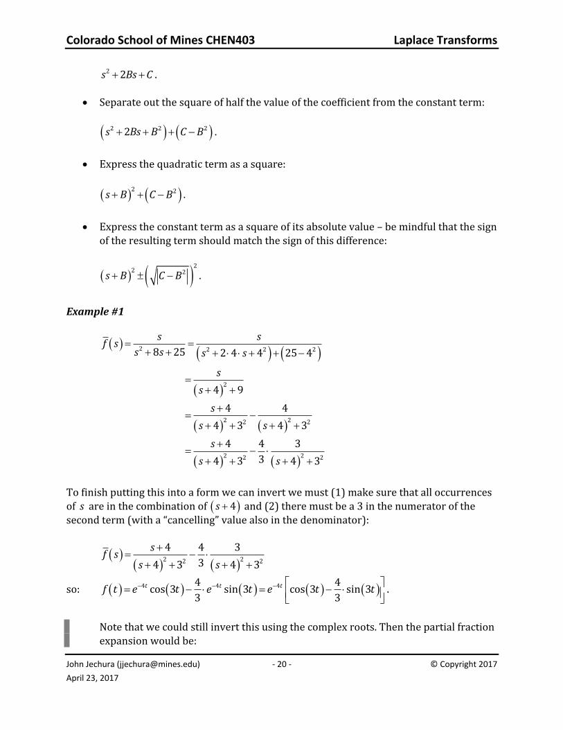
Example #1

2 2 2 2

2

2 22 2

2 22 2

8 25 2 4 4 25 4

4 9

4 4

4 3 4 3

4 4 3

34 3 4 3

s sf s

s s s s

s

s

s

s s

s

s s

To finish putting this into a form we can invert we must (1) make sure that all occurrences of s are in the combination of 4s and (2) there must be a 3 in the numerator of the second term (with a “cancelling” value also in the denominator):

2 22 2

4 4 3

34 3 4 3

sf s

s s

so:

4 4 44 4cos 3 sin 3 cos 3 sin 3

3 3t t tf t e t e t e t t .

Note that we could still invert this using the complex roots. Then the partial fraction

expansion would be:



April 23, 2017

2

1 3 4 1 3 4

8 25 6 4 3 6 4 3

s i if s

s s s i s i

3 4 3 4

exp 4 3 exp 4 36 6

i if t i t i t .

We can convert to trigonometric functions and eliminate the complex numbers:

4 3 3

4 3 3 3 3

4

3 4 3 4e e

6 6

1 2e e e e

2 3

4cos 3 sin 3

3

t i t i t

t i t i t i t i t

t

i if t e

ie

e t t

Numerical Root Finding & Partial Fractions

We may be presented with a transfer function that is of high polynomial order and does not

have analytical factors. We should not let this stand in the way of trying to solve the problem. After all, we are engineers and we are most interested in numerical solutions to our problems. The key step is the first step: finding the numerical roots to the polynomial in the denominator of the transfer function. Once these are found then there are multiple ways to find the terms in the numerators that represent the partial fractions. Inverting to the time domain is then an almost trivial matter. The technique can be shown with numerical examples. The calculations will all be shown using Microsoft Excel for the calculations. (The spreadsheet is available on the class web page.) All Real Roots

Let’s consider the transfer function:

5 4 3 2

1

9.2 33.15 58.3 49.85 16.495f s

s s s s s.



April 23, 2017

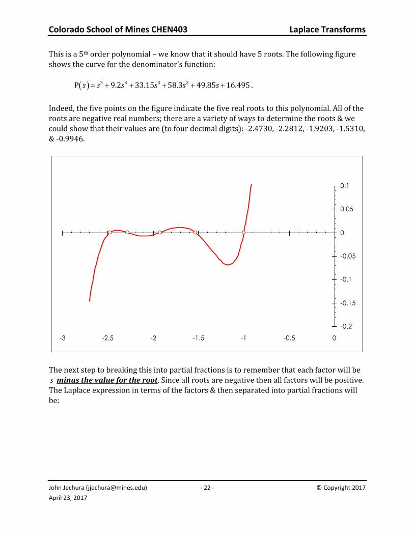
This is a 5th order polynomial – we know that it should have 5 roots. The following figure shows the curve for the denominator’s function:

5 4 3 2P 9.2 33.15 58.3 49.85 16.495s s s s s s .

Indeed, the five points on the figure indicate the five real roots to this polynomial. All of the roots are negative real numbers; there are a variety of ways to determine the roots & we could show that their values are (to four decimal digits): -2.4730, -2.2812, -1.9203, -1.5310, & -0.9946.

-0.2

-0.15

-0.1

-0.05

0

0.05

0.1

-3 -2.5 -2 -1.5 -1 -0.5 0

The next step to breaking this into partial fractions is to remember that each factor will be s minus the value for the root. Since all roots are negative then all factors will be positive. The Laplace expression in terms of the factors & then separated into partial fractions will be:



April 23, 2017

5 4 3 2

1

9.2 33.15 58.3 49.85 16.495

1

2.4730 2.2812 1.9203 1.5310 0.9946

2.4730 2.2812 1.9203 1.5310 0.9946

f ss s s s s

s s s s s

A B C D E

s s s s s

All coefficients can be determined using the Heaviside Expansion method. For example, for the first coefficient:

2.4730

1lim

2.2812 1.9203 1.5310 0.9946

1

2.4730 2.2812 2.4730 1.9203 2.4730 1.5310 2.4730 0.9946

6.774

sA

s s s s

Finding all coefficients in a similar manner gives:

5 4 3 2

1

9.2 33.15 58.3 49.85 16.495

6.774 14.967 13.910 6.776 1.059

2.4730 2.2812 1.9203 1.5310 0.9946

f ts s s s s

s s s s s

and the inverted result is:

6.774exp 2.4730 14.967exp 2.2812 13.910exp 1.9203

6.776exp 1.5310 1.059exp 0.9946

f s t t t

t t

The calculations are complicated to do by hand but are very doable using common computer tools (such as Excel). Complex Conjugate Roots

It doesn’t take much to turn a complicated numerical problem into a very complicated numerical problem. Let’s change our 5th order transfer function slightly in the last coefficient:



April 23, 2017

5 4 3 2

1

9.2 33.15 58.3 49.85 16.505f s

s s s s s.

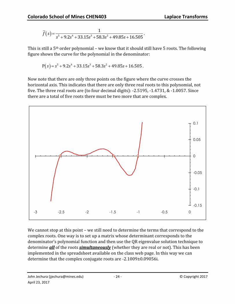
This is still a 5th order polynomial – we know that it should still have 5 roots. The following

figure shows the curve for the polynomial in the denominator:

5 4 3 2P 9.2 33.15 58.3 49.85 16.505s s s s s s .

Now note that there are only three points on the figure where the curve crosses the horizontal axis. This indicates that there are only three real roots to this polynomial, not five. The three real roots are (to four decimal digits): -2.5195, -1.4731, & -1.0057. Since there are a total of five roots there must be two more that are complex.

-0.15

-0.1

-0.05

0

0.05

0.1

-3 -2.5 -2 -1.5 -1 -0.5 0

We cannot stop at this point – we still need to determine the terms that correspond to the complex roots. One way is to set up a matrix whose determinant corresponds to the denominator’s polynomial function and then use the QR eigenvalue solution technique to determine all of the roots simultaneously (whether they are real or not). This has been implemented in the spreadsheet available on the class web page. In this way we can determine that the complex conjugate roots are -2.1009±0.09056i.



April 23, 2017

Now that we have all of the roots we can expand the Laplace function in the partial fraction form:

5 4 3 2

1

9.2 33.15 58.3 49.85 16.505

2.5195 1.4731 1.0057 2.1009 0.09056 2.1009 0.09056

f ss s s s s

A B C D E

s s s s i s i

All coefficients can be determined using the Heaviside Expansion method (even the complex ones). The coefficients for A , B , and C do not really require complex arithmetic since the product of the D & E factors lead to a quadratic expression with real coefficients. For example:

2.5195

22.5195

1lim

1.4731 1.0057 2.1009 0.09056 2.1009 0.09056

1lim

1.4731 1.0057 4.4218 4.2017

3.4422

s

s

As s s i s i

s s s s

Finding all of the coefficients in a similar manner gives:

5 4 3 2

1

9.2 33.15 58.3 49.85 16.505

3.4422 5.0830 1.1704 0.23527 18.496 0.23527 18.496

2.5195 1.4731 1.0057 2.1009 0.09056 2.1009 0.09056

f ss s s s s

i i

s s s s i s i

and the inverted result is:

2.5195 1.4731 1.0057

2.1009 0.09056 2.1009 0.09056

3.4422e 5.0830e 1.1704e

0.23527 18.496 e 0.23527 18.496 e

t t t

i t i t

f t

i i

The complex numbers can be eliminated by converting the last two exponential terms to trigonometric functions. Remember that the trigonometric functions can be related to exponentials by:

1

cos 2cos2

i i i ie e e e



April 23, 2017

sin 2sin2

i i i iie e i e e

So the resulting f t can be modified to trigonometric form as:

2.5195 1.4731 1.0057

2.1009 0.09056 0.09056

3.4422e 5.0830e 1.1704e

e 0.23527 18.496 e 0.23527 18.496 e

t t t

t i t i t

f t

i i

2.5195 1.4731 1.0057

2.1009 0.09056 0.09056 0.09056 0.09056

3.4422e 5.0830e 1.1704e

e 0.23527 e e 18.496 e e

t t t

t i t i t i t i t

f t

i

2.5195 1.4731 1.0057

2.1009

3.4422e 5.0830e 1.1704e

e 0.47053cos 0.09056 36.991sin 0.09056

t t t

t

f t

t t

The partial fraction coefficients for the complex conjugate terms will always be complex conjugates themselves when all of the coefficients in the Laplace function are real. This simplifies the transformation to trigonometric functions:

2 cos 2 sin

a i t a i t

at it it it it

at

A Bi A Bif s f t A Bi e A Bi e

s a i s a i

e A e e Bi e e

e A t B t

Note that one could also recombine the partial fractions involving the complex conjugate terms to give a single term with a quadratic in the denominator:

2 2 2

2 2

2

A Bi A Bif s

s a i s a i

A s aA B

s as a

which can be shown to invert to the same f t as before.



April 23, 2017

Solution of Initial Value ODEs

We can apply Laplace transforms to ODEs & obtain solutions. Example:

3 2

3 24 5 2 2

d x d x dxx

dt dt dt with

2

20 0

0 0t t

dx d xx

dt dt

.

Transforming:

3 2 2 2

0 0 0 4 0 0 5 0 2s x s x sx x s x sx x sx x xs

3 2 24 5 2s x s x sx x

s

3 2

2

4 5 2x s

s s s s

Again, the problem is to invert x s to get x t . We can factor the cubic term & then break apart into partial fractions:

2 2

2

2 11 2 1

A B C Dx s

s s ss s s s

The first three coefficients can easily be determined using the Heaviside Method to give:

2 2

2 1 1 2

2 11 2 1

Dx s

s s ss s s s.

We can determine the value of D by setting 1s to find 0D . So:

2 2

2 1 1 2

21 2 1x s

s ss s s s

which gives:

21 2t tx t e te .

Note that we have traded solving an ODE for factoring a polynomial and finding its partial fractions.



April 23, 2017

Further note:

22 2 2t t tdxe e te

dt

22

2

2

4 2 2 2

4 4 2

t t t t

t t t

d xe e e te

dt

e e te

32

3

2

8 4 2 2

8 6 2

t t t t

t t t

d xe e e te

dt

e e te

The ICs & the original ODE are satisfied by this solution.

Solution of Systems of Initial Value ODEs

We can also apply Laplace transforms to systems of ODEs & obtain solutions. Example:

1 11 2 1 2sin 2 2 2 sin

dy dyt y y y y t

dt dt

2 21 2 2 1 22 3 2 5 0

dy dyy y y y y

dt dt

with the ICs 1 20 0 0y y .

How would we even start to solve this without the special properties of Laplace transforms? The first step would be to eliminate one of the variables from one of the ODEs. For example, let’s eliminate 2y from the 1st ODE. We’ll start by rearranging the ODE to be in terms of 2y :

1 11 2 2 1

1 1sin 2 sin

2 2

dy dyt y y y y t

dt dt

and then by taking its derivative:

2

1 2 1 12 1 2

1 1 1 1sin cos

2 2 2 2

dy dy d y dyy y t t

dt dt dt dt.

Now, insert these two expressions into the 2nd ODE & re-arrange to give:



April 23, 2017

22 1 1 1

1 2 2 1 12

21 1

12

1 1 1 12 3 cos 2 5 sin

2 2 2 2

1 7 5 13 sin cos

2 2 2 2

dy d y dy dyy y y t y y t

dt dt dt dt

d y dyy t t

dt dt

Now, instead of two first order ODEs, we have one second order ODE. This means we also need to have to another IC on 1y . We can calculate the IC for the first derivative,

1 0/

ty dt , by inserting the 1 0y and 2 0y values into the original

form of the first ODE:

1 1 20 sin 0 2 0 0 0y y y .

Now we have the system in a form that we can try to solve it (either using Laplace transforms or some other technique).

It is much simpler to apply Laplace transforms and use algebraic equation techniques to solve this system of ODEs. Applying the Laplace transforms to the 1st equation gives:

11 2 1 1 1 22

1 2 2

1sin 2 0 2

1

12 2

1

dyt y y sy y y y

dt s

s y ys

and to the 2nd equation gives:

21 2 2 2 2 1 2 2

1 2

1 2

2 3 0 2 3

2 5 0

5

2

dyy y y sy y y y y

dt

y s y

sy y

Now we have a system of two algebraic equations in two unknowns. Inserting the 2nd equation into the 1st:

2 2 2

5 12 2

2 1

ss y y

s

22 2

27 6

1s s y

s



April 23, 2017

2 2 2 2

2 2

1 7 6 1 1 6y

s s s s s s

2 2

1 7 5 1 1 2 1

37 5 1 185 61

sy

s ss

2 2 2

7 5 1 1 1 2 1

37 37 5 1 185 61 1

sy

s ss s

62

7 5 1 2cos sin

37 37 5 185t ty t t t e e

Note: 62 7 5 1 12sin cos

37 37 5 185t tdy

t t e edt

and the other function is:

1 2 2

5 5 2

2 2 1 1 6

s sy y

s s s

1 2

1 15 16 2 1 1 1

37 5 1 185 61

sy

s ss

1 2 2

15 16 1 2 1 1 1

37 37 5 1 185 61 1

sy

s ss s

61

15 16 2 1cos sin

37 37 5 185t ty t t t e e

Note: 61 15 16 2 6sin cos

37 37 5 185t tdy

t t e edt

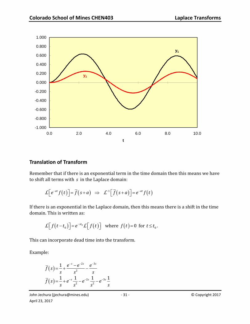
The following chart shows the two solutions.



April 23, 2017

-1.000

-0.800

-0.600

-0.400

-0.200

0.000

0.200

0.400

0.600

0.800

1.000

0.0 2.0 4.0 6.0 8.0 10.0

t

y1

y2

Translation of Transform

Remember that if there is an exponential term in the time domain then this means we have to shift all terms with s in the Laplace domain:

1at ate f t f s a f s a e f tL L

If there is an exponential in the Laplace domain, then this means there is a shift in the time domain. This is written as:

0

0

stf t t e f tL L where 0f t for 0t t .

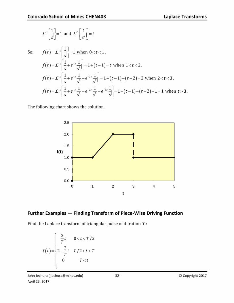
This can incorporate dead time into the transform. Example:

2 3

2

1 s s se e ef s

s s s

2 3

2 2

1 1 1 1s s sf s e e es s s s



April 23, 2017

1 11

sL and

1

2

1t

sL

So:

1 11f t

sL when 0 1t .

1

2

1 11 1sf t e t t

s sL when 1 2t .

1 2

2 2

1 1 11 1 2 2s sf t e e t t

s s sL when 2 3t .

1 2 3

2 2

1 1 1 11 1 2 1 1s s sf t e e e t t

s s s sL when 3t .

The following chart shows the solution.

0.0

0.5

1.0

1.5

2.0

2.5

0 1 2 3 4 5

t

f(t)

Further Examples — Finding Transform of Piece-Wise Driving Function

Find the Laplace transform of triangular pulse of duration T :

20 /2

22 /2

0

t t TT

f t t T t TT

T t



April 23, 2017

Brute Force Method. Can find directly from defining formula:

/2

0 0 /2

2 22 0

T Tst st st st

T T

t tf t f t e dt e dt e dt e dt

T TL

/2

0 /2 /2

2 22

T T Tst st st

T Tf t te dt e dt te dt

T TL

/2

2 2

/20 /2

1 12 22

T TTst stst

T T

e st e stef t

T s s T sL

/2

2 2

/2/2

2 2

12 12

112 2

2

sT

sTsTsT sT

sTe

f tT s s

sTe

e sTe e

s s T s s

L

/2 /2 /2

2 2 2

/2 /2

2 2 2 2

2 1 2

2

2

3

sT sT sT sT

sT sT sT sT

sTe e Te Tef t

T s s s T s s

sTe e sTe e

T s s s s

L

/2 /2 /2

2 2

/2 /2

2 2

2 1 2

2

2

2

sT sT sT sT

sT sT sT sT

Te e Te Tef t

T s s s T s s

Te e Te e

T s s s s

L

/2

2

21 2 sT sTf t e e

TsL

Alternate Method. Can also get this by recognizing that the original function can be re-written in terms of functions that “turn on” after a time delay:

1 2 32

Tf t f t f t f t T

Obviously:



April 23, 2017

1

2f t t

T

Over the 2nd range:

2 2 4 2 42 2

2

Tf t t t t t t

T T T T T

so:

2 2

4 4

2 2

T Tf t t f t t

T T

Over the final range:

2 2 2 4 20 2 2

2

Tf t t t t t t T

T T T T T

so: 3 3

2 2f t T t T f t t

T T

Now, we can take the Laplace transform of this function to get:

1 2 32

Tf t f t f t f t TL L L L

/2

1 2 3sT sTf t f t e f t e f tL L L L

/22 4 2sT sTf t t e t e tT T T

L L L L

/22 4 2sT sTf t t e t e t

T T TL L L L

/22 1 2 sT sTe ef t t

TL L

/2

2

2 1 2 sT sTe ef t

TsL

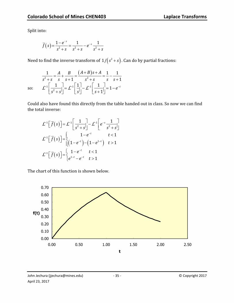
Further Examples — Inverse Transform With Time Delay

Find the inverse Laplace transform of:

2

1 sef s

s s



April 23, 2017

Split into:

2 2 2

1 1 1sse

f s es s s s s s

Need to find the inverse transform of 21/ s s . Can do by partial fractions:

2 2

1 1 1

1 1

A B s AA B

s s s s s s s s

so:

1 1 1

2

1 1 11

1te

s s s sL L L

Could also have found this directly from the table handed out in class. So now we can find the total inverse:

1 1 1

2 2

1 1sf s es s s s

L L L

1

1

1 1

1 1 1

t

t t

e tf s

e e tL

1

1

1 1

1

t

t t

e tf s

e e tL

The chart of this function is shown below.

0.00

0.10

0.20

0.30

0.40

0.50

0.60

0.70

0.00 0.50 1.00 1.50 2.00 2.50

t

f(t)



April 23, 2017

Further Examples — Arbitrary Driving Function in ODE

Consider the following ODE:

2

23 2

d f dff G t

dt dt

with the ICs

0 / 0

t of df dt and G t is an arbitrary driving function. The Laplace

transform of this system will be:

2 3 2s f s sf s f s G s

2 3 2 1 2

G s G sf s

s s s s

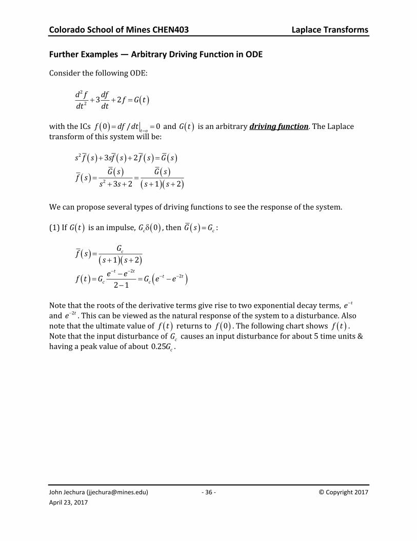
We can propose several types of driving functions to see the response of the system. (1) If G t is an impulse, 0cG , then cG s G :

1 2

cGf s

s s

22

2 1

t tt t

c c

e ef t G G e e

Note that the roots of the derivative terms give rise to two exponential decay terms, te and 2te . This can be viewed as the natural response of the system to a disturbance. Also note that the ultimate value of f t returns to 0f . The following chart shows f t . Note that the input disturbance of cG causes an input disturbance for about 5 time units & having a peak value of about 0.25 cG .



April 23, 2017

0.000

0.050

0.100

0.150

0.200

0.250

0.300

0.0 1.0 2.0 3.0 4.0 5.0

t

f(t)/Gc

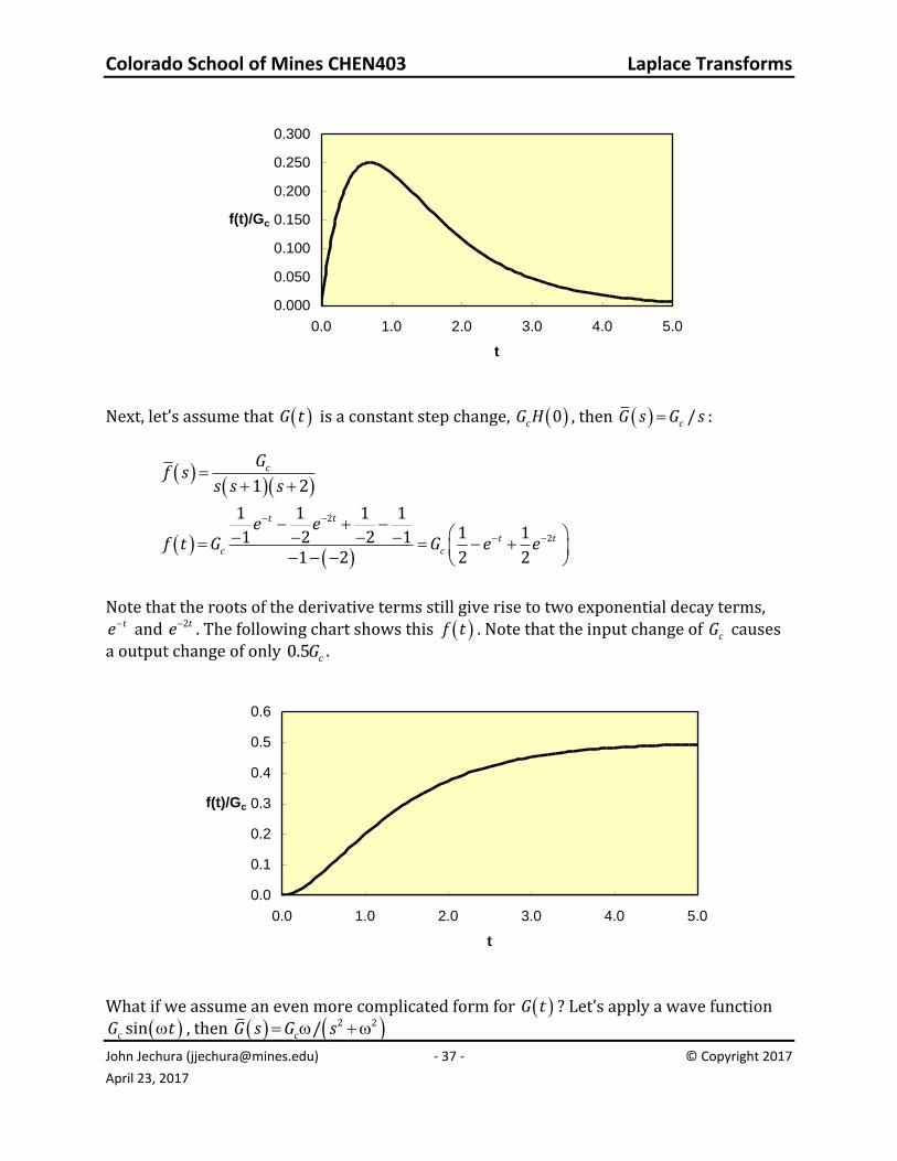
Next, let’s assume that G t is a constant step change, 0cG H , then /cG s G s :

1 2

cGf s

s s s

2

2

1 1 1 11 11 2 2 1

1 2 2 2

t t

t tc c

e ef t G G e e

Note that the roots of the derivative terms still give rise to two exponential decay terms,

te and 2te . The following chart shows this f t . Note that the input change of cG causes a output change of only 0.5 cG .

0.0

0.1

0.2

0.3

0.4

0.5

0.6

0.0 1.0 2.0 3.0 4.0 5.0

t

f(t)/Gc

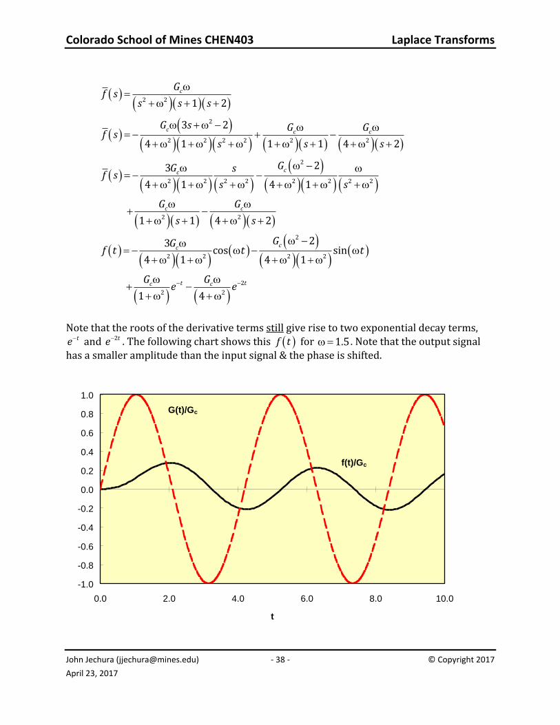
What if we assume an even more complicated form for G t ? Let’s apply a wave function

sincG t , then 2 2/cG s G s



April 23, 2017

2 2

2

2 2 2 2 2 2

2

2 2 2 2 2 2 2 2

2 2

1 2

3 2

4 1 1 1 4 2

23

4 1 4 1

1 1 4 2

c

c c c

cc

c c

Gf s

s s s

G s G Gf s

s s s

GG sf s

s s

G G

s s

2

2 2 2 2

2

2 2

23cos sin

4 1 4 1

1 4

cc

t tc c

GGf t t t

G Ge e

Note that the roots of the derivative terms still give rise to two exponential decay terms,

te and 2te . The following chart shows this f t for 1.5 . Note that the output signal has a smaller amplitude than the input signal & the phase is shifted.

-1.0

-0.8

-0.6

-0.4

-0.2

0.0

0.2

0.4

0.6

0.8

1.0

0.0 2.0 4.0 6.0 8.0 10.0

t

G(t)/Gc

f(t)/Gc



April 23, 2017

Use of Mathematical Software to Work with Laplace Transforms

Specialized mathematical software can be used to do all of the operations discussed here — splitting apart a Laplace function into partial fractions and then inverting to the t domain

or even doing the inversion in one step. Two examples of this software are Mathematica and MATLAB. In fact, if one narrows their focus on the type of problem to be solved, even software such as Microsoft® Excel and POLYMATH can be used However, it is strongly recommended that in the beginning the student practice doing the operations on his/her own and not rely solely on this software (if for no other reason than computers with this software will not be available to the student during quizzes and exams). Mathematica

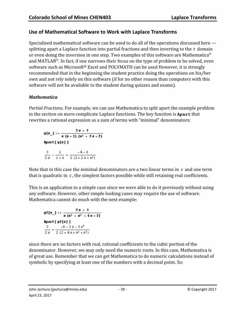
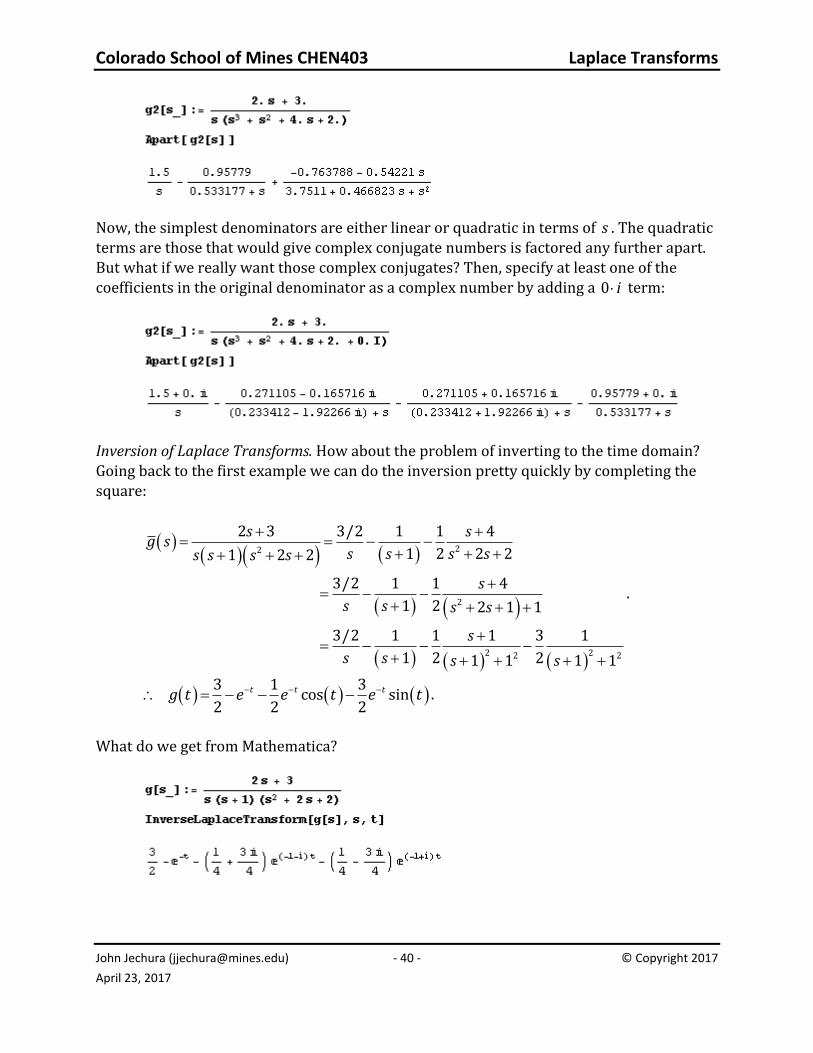
Partial Fractions. For example, we can use Mathematica to split apart the example problem in the section on more complicate Laplace functions. The key function is Apart that rewrites a rational expression as a sum of terms with “minimal” denominators:

Note that in this case the minimal denominators are a two linear terms in s and one term that is quadratic in s , the simplest factors possible while still retaining real coefficients. This is an application to a simple case since we were able to do it previously without using any software. However, other simple looking cases may require the use of software. Mathematica cannot do much with the next example:

since there are no factors with real, rational coefficients to the cubic portion of the denominator. However, we may only need the numeric roots. In this case, Mathematica is of great use. Remember that we can get Mathematica to do numeric calculations instead of symbolic by specifying at least one of the numbers with a decimal point. So:



April 23, 2017

Now, the simplest denominators are either linear or quadratic in terms of s . The quadratic terms are those that would give complex conjugate numbers is factored any further apart. But what if we really want those complex conjugates? Then, specify at least one of the coefficients in the original denominator as a complex number by adding a 0 i term:

Inversion of Laplace Transforms. How about the problem of inverting to the time domain? Going back to the first example we can do the inversion pretty quickly by completing the square:

22

2

2 22 2

2 3 3/2 1 1 4

1 2 2 21 2 2

3/2 1 1 4

1 2 2 1 1

3/2 1 1 1 3 1

1 2 21 1 1 1

s sg s

s s s ss s s s

s

s s s s

s

s s s s

.

3 1 3

cos sin2 2 2

t t tg t e e t e t .

What do we get from Mathematica?



April 23, 2017

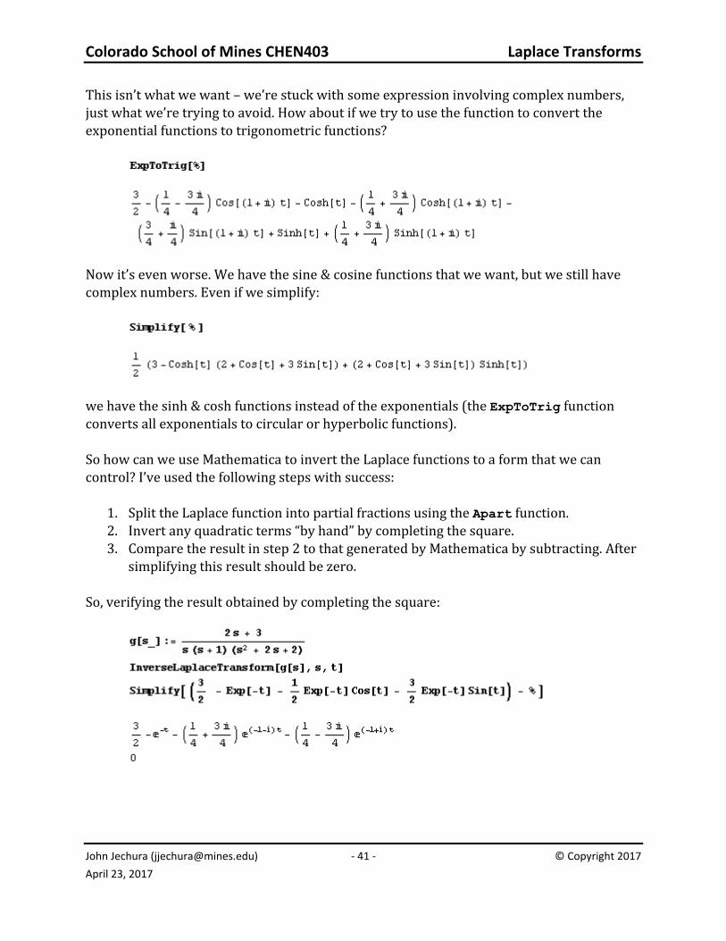
This isn’t what we want – we’re stuck with some expression involving complex numbers, just what we’re trying to avoid. How about if we try to use the function to convert the exponential functions to trigonometric functions?

Now it’s even worse. We have the sine & cosine functions that we want, but we still have complex numbers. Even if we simplify:

we have the sinh & cosh functions instead of the exponentials (the ExpToTrig function converts all exponentials to circular or hyperbolic functions). So how can we use Mathematica to invert the Laplace functions to a form that we can control? I’ve used the following steps with success:

1. Split the Laplace function into partial fractions using the Apart function. 2. Invert any quadratic terms “by hand” by completing the square. 3. Compare the result in step 2 to that generated by Mathematica by subtracting. After

simplifying this result should be zero. So, verifying the result obtained by completing the square:



April 23, 2017

MATLAB

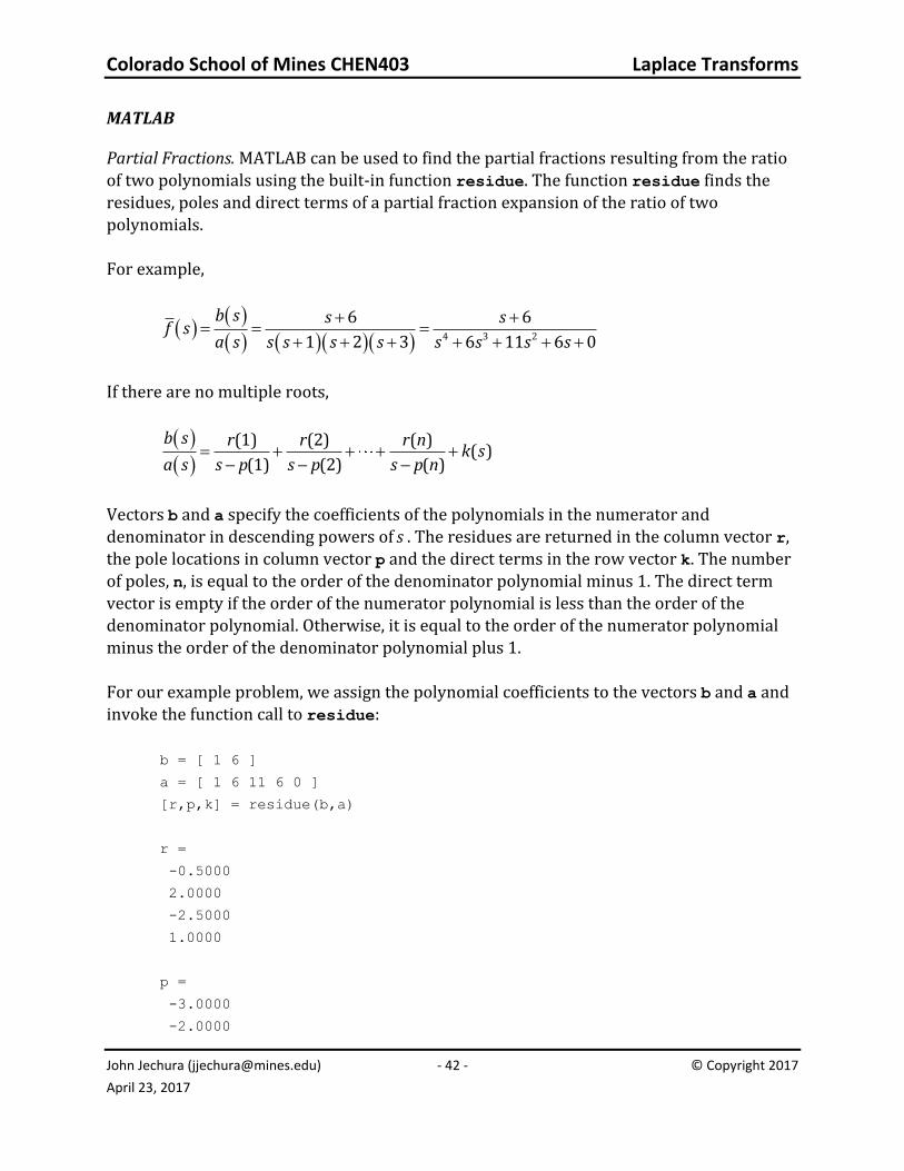
Partial Fractions. MATLAB can be used to find the partial fractions resulting from the ratio of two polynomials using the built-in function residue. The function residue finds the

residues, poles and direct terms of a partial fraction expansion of the ratio of two polynomials. For example,

4 3 2

6 6

1 2 3 6 11 6 0

b s s sf s

a s s s s s s s s s

If there are no multiple roots,

(1) (2) ( )( )

(1) (2) ( )

b s r r r nk s

a s s p s p s p n

Vectors b and a specify the coefficients of the polynomials in the numerator and denominator in descending powers of s . The residues are returned in the column vector r, the pole locations in column vector p and the direct terms in the row vector k. The number of poles, n, is equal to the order of the denominator polynomial minus 1. The direct term vector is empty if the order of the numerator polynomial is less than the order of the

denominator polynomial. Otherwise, it is equal to the order of the numerator polynomial minus the order of the denominator polynomial plus 1. For our example problem, we assign the polynomial coefficients to the vectors b and a and invoke the function call to residue:

b = [ 1 6 ]

a = [ 1 6 11 6 0 ]

[r,p,k] = residue(b,a)

r =

-0.5000

2.0000

-2.5000

1.0000

p =

-3.0000

-2.0000



April 23, 2017

-1.0000

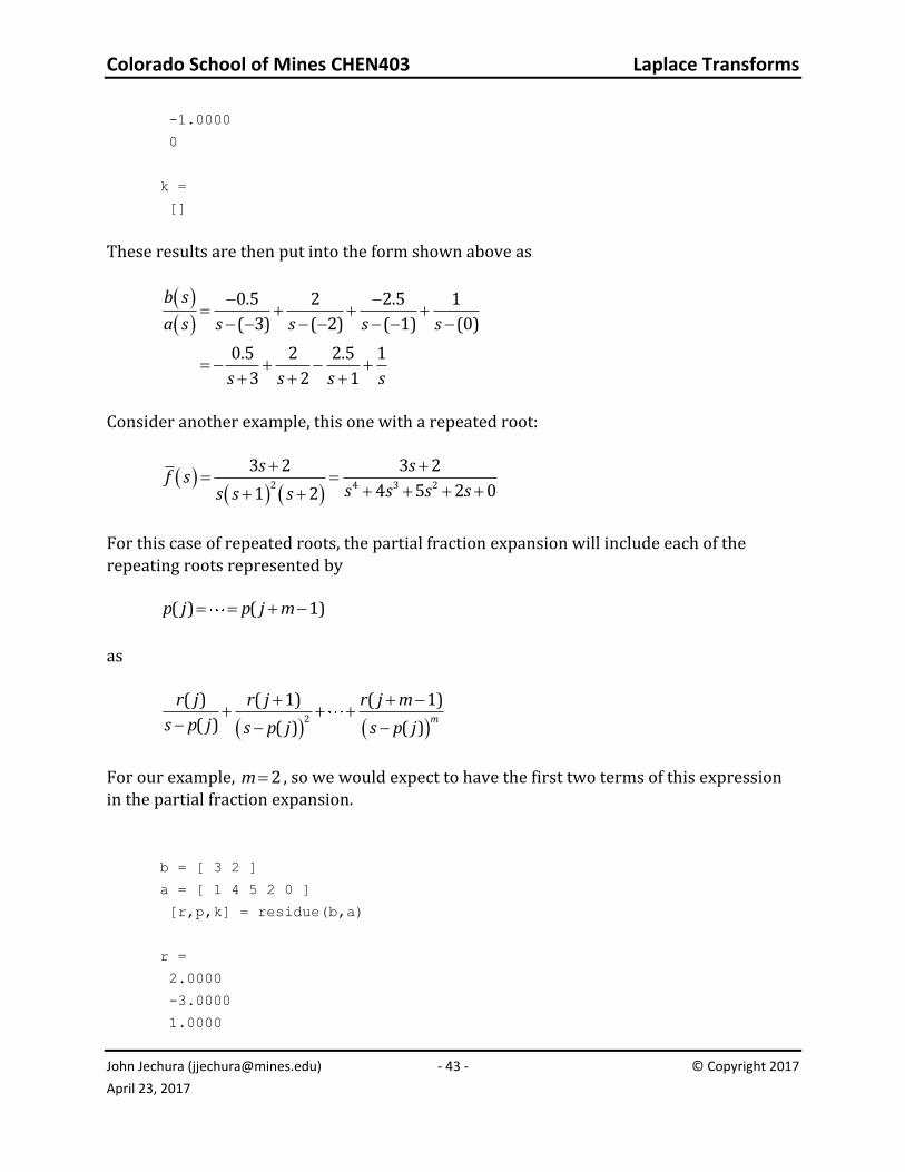
0

k =

[]

These results are then put into the form shown above as

0.5 2 2.5 1

( 3) ( 2) ( 1) (0)

0.5 2 2.5 1

3 2 1

b s

a s s s s s

s s s s

Consider another example, this one with a repeated root:

2 4 3 2

3 2 3 2

4 5 2 01 2

s sf s

s s s ss s s

For this case of repeated roots, the partial fraction expansion will include each of the repeating roots represented by ( ) ( 1)p j p j m

as

2

( ) ( 1) ( 1)

( ) ( ) ( )m

r j r j r j m

s p j s p j s p j

For our example, 2m , so we would expect to have the first two terms of this expression in the partial fraction expansion.

b = [ 3 2 ]

a = [ 1 4 5 2 0 ]


r =

2.0000

-3.0000

1.0000



April 23, 2017

1.0000

p =

-2.0000

-1.0000

-1.0000

0

k =

[]

These results are put into the form shown above as:

2

2

2 3 1 1

( 2) ( 1) (0)( 1)

2 3 1 1

2 1 ( 1)

b s

a s s s ss

s s s s

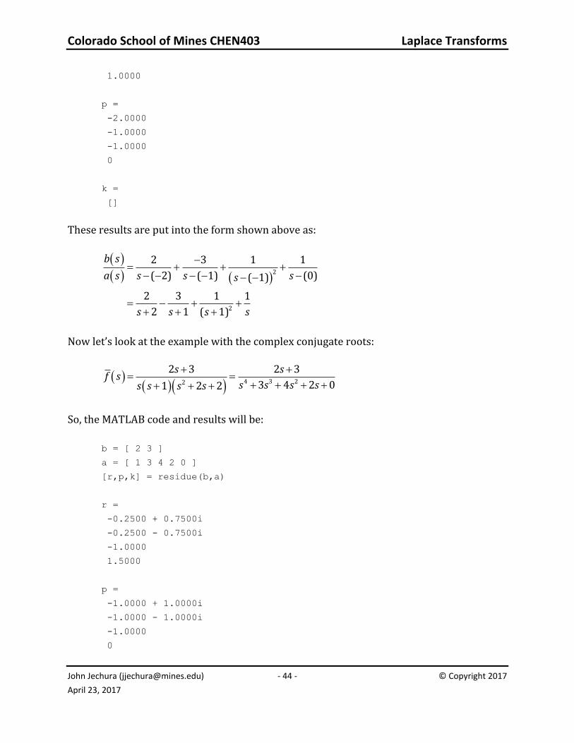
Now let’s look at the example with the complex conjugate roots:

4 3 22

2 3 2 3

3 4 2 01 2 2

s sf s

s s s ss s s s

So, the MATLAB code and results will be:

b = [ 2 3 ]

a = [ 1 3 4 2 0 ]


r =

-0.2500 + 0.7500i

-0.2500 - 0.7500i

-1.0000

1.5000

p =

-1.0000 + 1.0000i

-1.0000 - 1.0000i

-1.0000

0



April 23, 2017

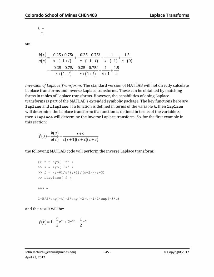
k =

[]

so:

0.25 0.75 0.25 0.75 1 1.5

( 1 ) ( 1 ) ( 1) (0)

0.25 0.75 0.25 0.75 1 1.5

1 1 1

b s i i

a s s i s i s s

i i

s i s i s s

Inversion of Laplace Transforms. The standard version of MATLAB will not directly calculate Laplace transforms and inverse Laplace transforms. These can be obtained by matching forms in tables of Laplace transforms. However, the capabilities of doing Laplace transforms is part of the MATLAB’s extended symbolic package. The key functions here are laplace and ilaplace. If a function is defined in terms of the variable t, then laplace will determine the Laplace transform; if a function is defined in terms of the variable s, then ilaplace will determine the inverse Laplace transform. So, for the first example in this section:

6

1 2 3

b s sf s

a s s s s s

the following MATLAB code will perform the inverse Laplace transform:

>> f = sym( 'f' )

>> s = sym( 's' )

>> f = (s+6)/s/(s+1)/(s+2)/(s+3)

>> ilaplace( f )

ans =

1-5/2*exp(-t)+2*exp(-2*t)-1/2*exp(-3*t)

and the result will be:

2 35 11 2

2 2t t tf t e e e .



April 23, 2017

Microsoft Excel

Excel can be used to perform the final calculations and create plots, but these capabilities will not be addressed here. Without customization Excel has limited capabilities to break

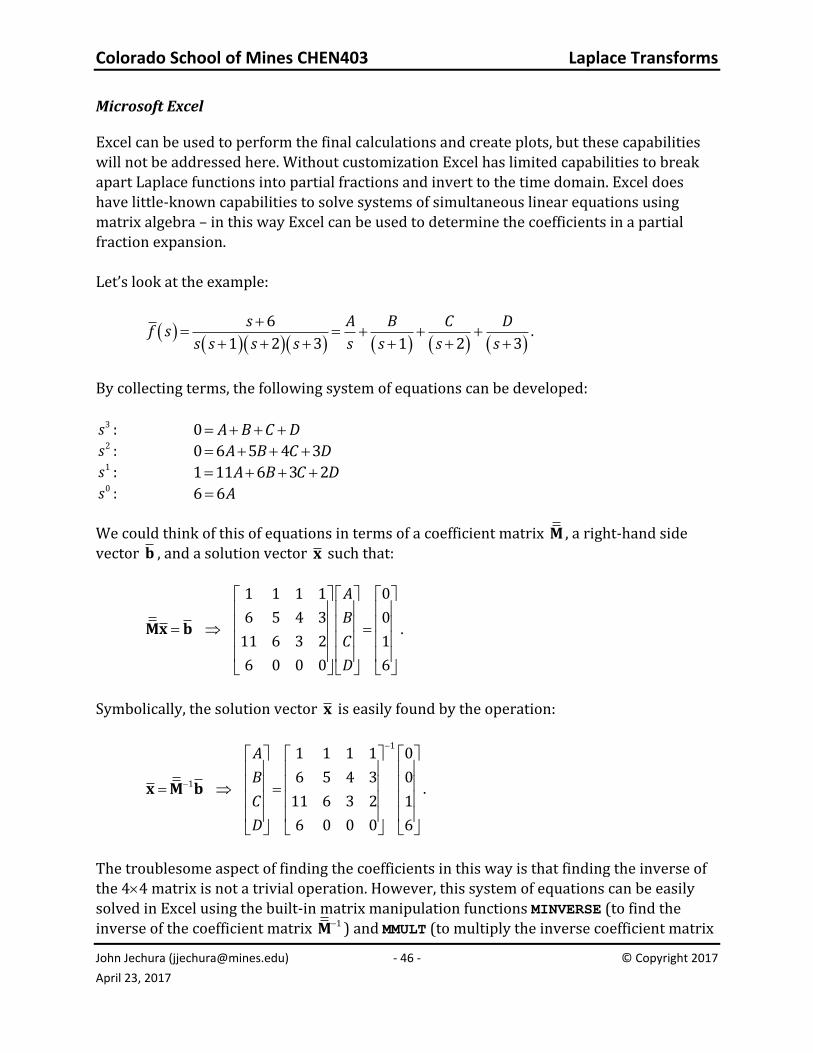
apart Laplace functions into partial fractions and invert to the time domain. Excel does have little-known capabilities to solve systems of simultaneous linear equations using matrix algebra – in this way Excel can be used to determine the coefficients in a partial fraction expansion. Let’s look at the example:

6

1 2 3 1 2 3

s A B C Df s

s s s s s s s s.

By collecting terms, the following system of equations can be developed:

3s : 0 A B C D 2s : 0 6 5 4 3A B C D 1s : 1 11 6 3 2A B C D 0s : 6 6A

We could think of this of equations in terms of a coefficient matrix M , a right-hand side

vector b , and a solution vector x such that:

1 1 1 1 0

6 5 4 3 0

11 6 3 2 1

6 0 0 0 6

A

B

C

D

Mx b .

Symbolically, the solution vector x is easily found by the operation:

1

1

1 1 1 1 0

6 5 4 3 0

11 6 3 2 1

6 0 0 0 6

A

B

C

D

x M b .

The troublesome aspect of finding the coefficients in this way is that finding the inverse of the 44 matrix is not a trivial operation. However, this system of equations can be easily solved in Excel using the built-in matrix manipulation functions MINVERSE (to find the

inverse of the coefficient matrix 1M ) and MMULT (to multiply the inverse coefficient matrix



April 23, 2017

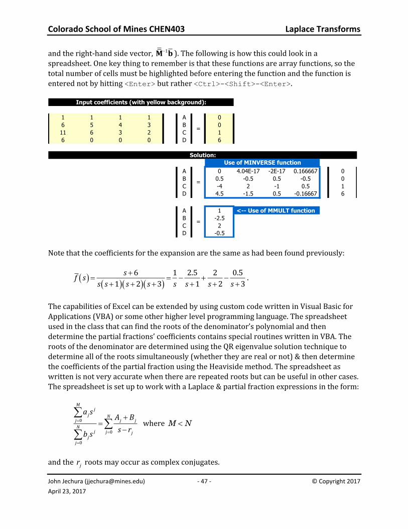
and the right-hand side vector, 1M b ). The following is how this could look in a spreadsheet. One key thing to remember is that these functions are array functions, so the total number of cells must be highlighted before entering the function and the function is entered not by hitting <Enter> but rather <Ctrl>-<Shift>-<Enter>.

1 1 1 1 A 0

6 5 4 3 B 0

11 6 3 2 C 1

6 0 0 0 D 6

A 0 4.04E-17 -2E-17 0.166667 0

B 0.5 -0.5 0.5 -0.5 0

C -4 2 -1 0.5 1

D 4.5 -1.5 0.5 -0.16667 6

A 1

B -2.5

C 2

D -0.5

=

=

=

Input coefficients (with yellow background):

Solution:

Use of MINVERSE function

<-- Use of MMULT function

Note that the coefficients for the expansion are the same as had been found previously:

6 1 2.5 2 0.5

1 2 3 1 2 3

sf s

s s s s s s s s.

The capabilities of Excel can be extended by using custom code written in Visual Basic for Applications (VBA) or some other higher level programming language. The spreadsheet used in the class that can find the roots of the denominator’s polynomial and then determine the partial fractions’ coefficients contains special routines written in VBA. The roots of the denominator are determined using the QR eigenvalue solution technique to determine all of the roots simultaneously (whether they are real or not) & then determine the coefficients of the partial fraction using the Heaviside method. The spreadsheet as written is not very accurate when there are repeated roots but can be useful in other cases. The spreadsheet is set up to work with a Laplace & partial fraction expressions in the form:

0

0

0

Mj

j Nj j j

Nj j j

jj

a sA B

s rb s

where M N

and the jr roots may occur as complex conjugates.



April 23, 2017

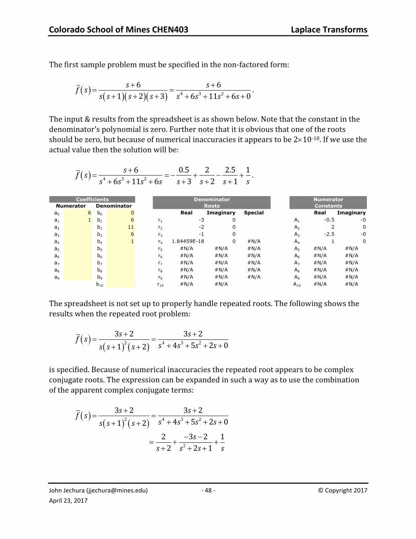
The first sample problem must be specified in the non-factored form:

4 3 2

6 6

1 2 3 6 11 6 0

s sf s

s s s s s s s s.

The input & results from the spreadsheet is as shown below. Note that the constant in the denominator’s polynomial is zero. Further note that it is obvious that one of the roots should be zero, but because of numerical inaccuracies it appears to be 210-18. If we use the actual value then the solution will be:

4 3 2

6 0.5 2 2.5 1

6 11 6 3 2 1

sf s

s s s s s s s s.

a0 6 b0 0 Real Imaginary Special Real Imaginary

a1 1 b1 6 r1 -3 0 A1 -0.5 -0

a2 b2 11 r2 -2 0 A2 2 0

a3 b3 6 r3 -1 0 A3 -2.5 -0

a4 b4 1 r4 1.84459E-18 0 #N/A A4 1 0

a5 b5 r5 #N/A #N/A #N/A A5 #N/A #N/A

a6 b6 r6 #N/A #N/A #N/A A6 #N/A #N/A

a7 b7 r7 #N/A #N/A #N/A A7 #N/A #N/A

a8 b8 r8 #N/A #N/A #N/A A8 #N/A #N/A

a9 b9 r9 #N/A #N/A #N/A A9 #N/A #N/A

b10 r10 #N/A #N/A A10 #N/A #N/A

Roots

Numerator

Constants

Coefficients

Numerator Denominator

Denominator

The spreadsheet is not set up to properly handle repeated roots. The following shows the results when the repeated root problem:

2 4 3 2

3 2 3 2

4 5 2 01 2

s sf s

s s s ss s s

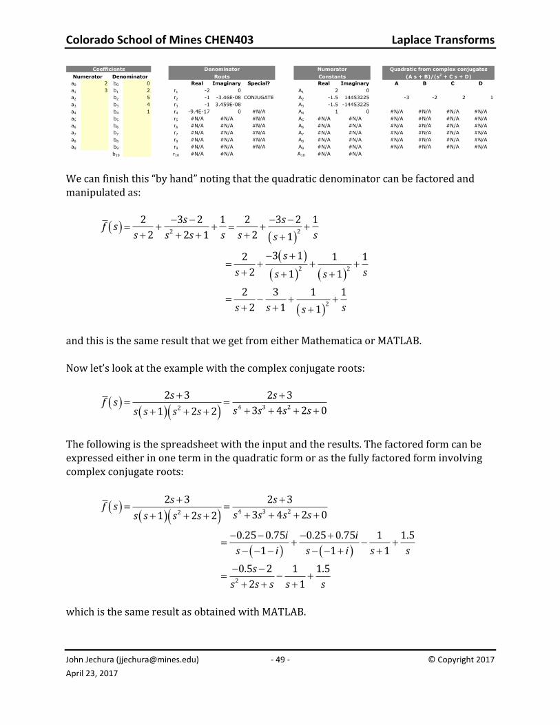
is specified. Because of numerical inaccuracies the repeated root appears to be complex conjugate roots. The expression can be expanded in such a way as to use the combination of the apparent complex conjugate terms:

2 4 3 2

2

3 2 3 2

4 5 2 01 2

2 3 2 1

2 2 1

s sf s

s s s ss s s

s

s s s s



April 23, 2017

a0 2 b0 0 Real Imaginary Special? Real Imaginary A B C D

a1 3 b1 2 r1 -2 0 A1 2 0

a2 b2 5 r2 -1 -3.46E-08 CONJUGATE A2 -1.5 14453225 -3 -2 2 1

a3 b3 4 r3 -1 3.459E-08 A3 -1.5 -14453225

a4 b4 1 r4 -9.4E-17 0 #N/A A4 1 0 #N/A #N/A #N/A #N/A

a5 b5 r5 #N/A #N/A #N/A A5 #N/A #N/A #N/A #N/A #N/A #N/A





b10 r10 #N/A #N/A A10 #N/A #N/A

Coefficients


Denominator Quadratic from complex conjugates

(A s + B)/(s2 + C s + D)Roots

Numerator

Constants

We can finish this “by hand” noting that the quadratic denominator can be factored and manipulated as:

22

2 2

2

2 3 2 1 2 3 2 1

2 2 1 2 1

3 12 1 1

2 1 1

2 3 1 1

2 1 1

s sf s

s s s s s ss

s

s ss s

s s ss

and this is the same result that we get from either Mathematica or MATLAB. Now let’s look at the example with the complex conjugate roots:

4 3 22

2 3 2 3

3 4 2 01 2 2

s sf s

s s s ss s s s

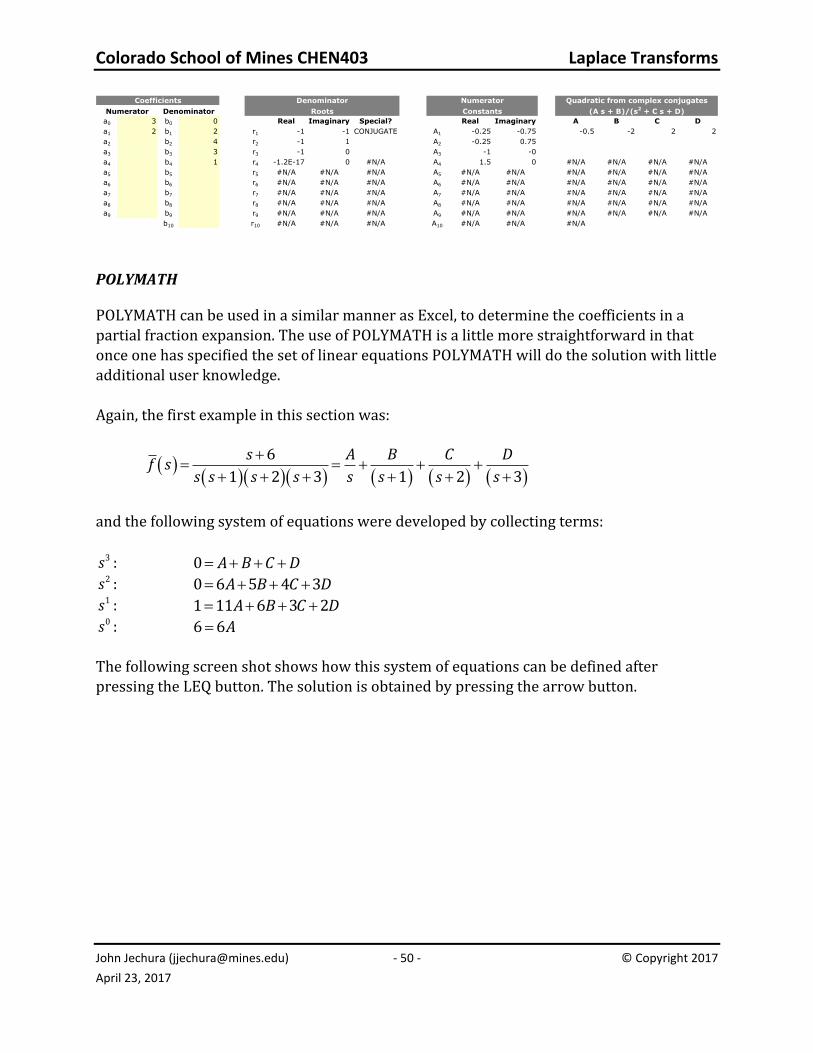
The following is the spreadsheet with the input and the results. The factored form can be expressed either in one term in the quadratic form or as the fully factored form involving

complex conjugate roots:

4 3 22

2

2 3 2 3

3 4 2 01 2 2

0.25 0.75 0.25 0.75 1 1.5

1 1 1

0.5 2 1 1.5

2 1

s sf s

s s s ss s s s

i i

s i s i s s

s

s s s s s

which is the same result as obtained with MATLAB.



April 23, 2017

a0 3 b0 0 Real Imaginary Special? Real Imaginary A B C D

a1 2 b1 2 r1 -1 -1 CONJUGATE A1 -0.25 -0.75 -0.5 -2 2 2

a2 b2 4 r2 -1 1 A2 -0.25 0.75

a3 b3 3 r3 -1 0 A3 -1 -0

a4 b4 1 r4 -1.2E-17 0 #N/A A4 1.5 0 #N/A #N/A #N/A #N/A






b10 r10 #N/A #N/A #N/A A10 #N/A #N/A #N/A

Quadratic from complex conjugates

(A s + B)/(s2 + C s + D)Roots

Numerator

Constants

Coefficients


Denominator

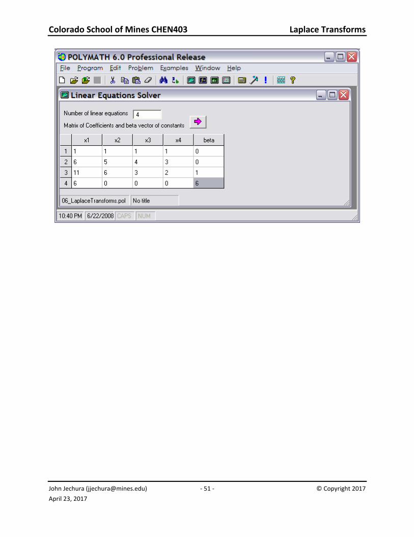
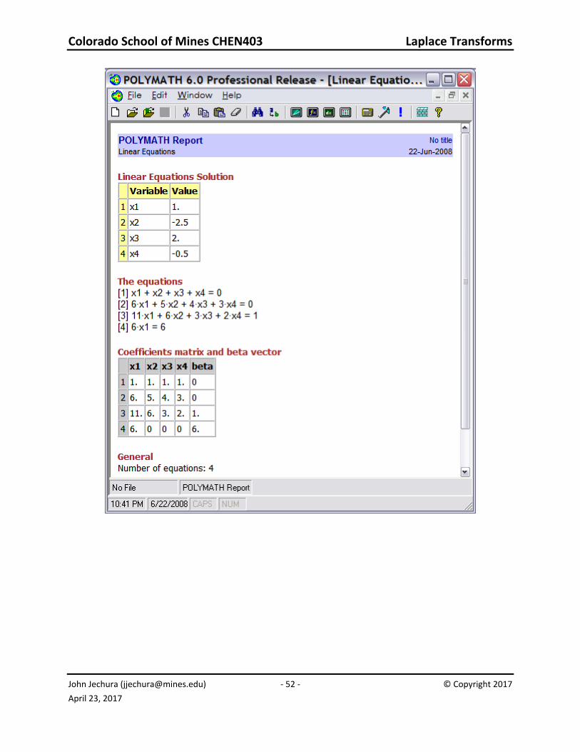
POLYMATH

POLYMATH can be used in a similar manner as Excel, to determine the coefficients in a partial fraction expansion. The use of POLYMATH is a little more straightforward in that once one has specified the set of linear equations POLYMATH will do the solution with little

additional user knowledge. Again, the first example in this section was:

6

1 2 3 1 2 3

s A B C Df s

s s s s s s s s

and the following system of equations were developed by collecting terms:

3s : 0 A B C D 2s : 0 6 5 4 3A B C D 1s : 1 11 6 3 2A B C D 0s : 6 6A

The following screen shot shows how this system of equations can be defined after pressing the LEQ button. The solution is obtained by pressing the arrow button.



April 23, 2017



April 23, 2017

Documents

Colorado School of Mines CHEN403 Laplace …inside.mines.edu/~jjechura/ProcessDynamics/05_LaplaceTransforms.pdfColorado School of Mines CHEN403 Laplace Transforms . = = = . ¦ ¦ ¦